Compressive Detection of Random Subspace Signals

Alireza Razavi, Mikko Valkama, and Danijela Cabric A. Razavi and M. Valkama are with the Department of Electronics and Communications Engineering, Tampere University of Technology (TUT), Tampere, Finland. emails: alireza.razavi@tut.fi, mikko.e.valkama@tut.fi.D. Cabric is with Cognitive Reconfigurable Embedded Systems Lab (CORES), University of California Los Angeles (UCLA), CA. email:danijela@ee.ucla.edu.
Abstract

The problem of compressive detection of random subspace signals is studied. We consider signals modeled as 𝐬=𝐇𝐱𝐬𝐇𝐱\mathbf{s}=\mathbf{H}\mathbf{x} where 𝐇𝐇\mathbf{H} is an N×K𝑁𝐾N\times K matrix with KN𝐾𝑁K\leq N and 𝐱𝒩(𝟎K,1,σx2𝐈K)similar-to𝐱𝒩subscript0𝐾1superscriptsubscript𝜎𝑥2subscript𝐈𝐾\mathbf{x}\sim\mathcal{N}(\mathbf{0}_{K,1},\sigma_{x}^{2}\mathbf{I}_{K}). We say that signal 𝐬𝐬\mathbf{s} lies in or leans toward a subspace if the largest eigenvalue of 𝐇𝐇Tsuperscript𝐇𝐇𝑇\mathbf{H}\mathbf{H}^{T} is strictly greater than its smallest eigenvalue. We first design a measurement matrix 𝚽=[𝚽sT,𝚽oT]T𝚽superscriptsuperscriptsubscript𝚽𝑠𝑇superscriptsubscript𝚽𝑜𝑇𝑇\mbox{\boldmath$\Phi$\unboldmath}=[\mbox{\boldmath$\Phi$\unboldmath}_{s}^{T},\mbox{\boldmath$\Phi$\unboldmath}_{o}^{T}]^{T} comprising of two sub-matrices 𝚽ssubscript𝚽𝑠\mbox{\boldmath$\Phi$\unboldmath}_{s} and 𝚽osubscript𝚽𝑜\mbox{\boldmath$\Phi$\unboldmath}_{o} where 𝚽ssubscript𝚽𝑠\mbox{\boldmath$\Phi$\unboldmath}_{s} projects the signal to the strongest left-singular vectors, i.e., the left-singular vectors corresponding to the largest singular values, of subspace matrix 𝐇𝐇\mathbf{H} and 𝚽osubscript𝚽𝑜\mbox{\boldmath$\Phi$\unboldmath}_{o} projects it to the weakest left-singular vectors. We then propose two detectors which work based on the difference in energies of the samples measured by the two sub-matrices 𝚽ssubscript𝚽𝑠\mbox{\boldmath$\Phi$\unboldmath}_{s} and 𝚽osubscript𝚽𝑜\mbox{\boldmath$\Phi$\unboldmath}_{o} and provide theoretical proofs for their optimality. Simplified versions of the proposed detectors for the case when the variance of noise is known are also provided. Furthermore, we study the performance of the detector when measurements are imprecise and show how imprecision can be compensated by employing more measurement devices. The problem is then re-formulated for the generalized case when the signal lies in the union of a finite number of linear subspaces instead of a single linear subspace. Finally, we study the performance of the proposed methods by simulation examples.

Index Terms:
Compressive Detection, Random Subspace Signals, Hypothesis Testing, Unknown Noise Variance, F𝐹F-distribution

I Introduction

The topic of Compressive Sensing (CS), where the effort is to draw inferences about the sparse signals based on compressive samples, has been one of the most attractive topics in the area of signal processing for more than a decade. Compressive Sensing states that if a signal is sparse in some known bases, then it is possible to reconstruct it from a relatively few linear projections [1, 2, 3]. While most of the efforts in the area of CS has been devoted to the problem of estimation of a sparse signal from possibly noisy compressive measurements, there have been also some efforts in accomplishing other signal processing tasks such as Compressive Detection [4, 5, 6, 7, 8, 9, 10, 11, 12], Compressive Classification [13, 14, 15, 4, 16], etc. The goal of this paper is to study the problem of detecting a random subspace signal from its compressive measurements.

Signal detection [17] is an important task in Statistical Signal Processing where the goal is to decide on the presence/absence of a signal rather than estimating it. Signal Detection has applications in many areas of engineering and science, including wireless communications, radar and sonar, bioinformatics, etc. The literature on detection from classical uncompressed samples is very vast and well-studied; see, e.g., [17, 18, 19] and references therein. With the advent of compressive sampling methods, like many other fields, there have been additional efforts to tailor the existing signal detection techniques to the case where the samples are taken at compressive rates. The first criterion that a signal has to meet to qualify for being detectable based on compressive samples is to be sparse in some known basis, or in a broader sense to lie in a low-dimensional subspace of the higher-dimensional ambient space. The applications of such compressive detection techniques are in the scenarios where uncompressed sampling is difficult, expensive, or even harmful, but because of the existence of a structure in the signal we are still able to sample the signal in compressive rate and then detect it based on the compressive samples. Examples of such scenarios are compressive spectrum sensing of OFDM signals [20, 21], radar sensing [22, 23, 24, 25], hyperspectral imaging [26], ultrasound imaging [27], etc. We remark here that the hardware implementation of specific compressive samplers is beyond the scope of this paper and we only focus on finding the optimal mathematical model or framework of such samplers, however examples of hardware implementations in various applications can be found in [28, 29, 30, 27, 22, 31, 32, 33].

In this paper we address the problem of compressive detection of signals that lie on or close to a low dimensional linear subspace. We start with the simplest case when the signal is drawn from a known low-dimensional subspace and propose two tests for detection of signal from compressive measurements. The main advantage of the proposed algorithms over the existing methods is that they do not need the knowledge of the noise variance to work. However, we also provide the simplified versions of the proposed methods for the case when the noise variance is known. We then study the effect of imprecise measurements and show that the imprecision can be compensated by employing more measurement devices. Then the proposed method is re-formulated for the case when the signal is lying on the union of a finite number of known linear subspaces with each of subspaces having a certain probability of being the subspace on which the signal truly lies. In other words, in this case, instead of having the exact knowledge of the subspace, we know the set of all subspaces from which the signal may emerge together with the corresponding probabilities that the signal may lie on each of them. We will introduce the optimum sampling strategy in this case and show that although the performance falls by increasing the number of possible subspaces, it remains reasonable as long as the cardinality of the set is much smaller than the ambient dimension.

Related work: In [4, 5, 6, 12] authors studied the problem of compressive detection, but they formulated the problem for deterministic agnostic signals rather than random subspace signals. Besides, their methods did not take into consideration the unknown noise variance scenario. The method in [7] designs a matched subspace detector for subspace signals. The method assumes that the exact knowledge of signal is available for detector design. They extend their work to unknown signals in [8] but like the previous ones they need the variance of noise to design the compressive detector. The work of [10] provided upper bounds for probabilities of false alarm and mis-detection for deterministic signals while the variance of noise is again assumed known. Finally, in [11] authors studied the problem of compressive detection of random subspace signals but similar to the previously mentioned works the noise variance was assumed known and the signal was assumed agnostic.

Notations and Mathematical Preliminaries: Throughout this paper, all quantities are assumed real-valued while matrices and vectors are denoted by capital and small boldface letters, respectively. == denotes the equality and \triangleq denotes the definition. 𝔼Xsubscript𝔼𝑋\mathbb{E}_{X} is reserved for statistical expectation operator with respect to the random variable X𝑋X, and tensor-product\otimes denotes the Kronecker product. 𝐈Psubscript𝐈𝑃\mathbf{I}_{P}, 𝟏P,Qsubscript1𝑃𝑄\mathbf{1}_{P,Q} and 𝟎P,Qsubscript0𝑃𝑄\mathbf{0}_{P,Q} represent P×P𝑃𝑃P\times P identity matrix, and P×Q𝑃𝑄P\times Q all-one and all-zero matrices, respectively. The set of real numbers is denoted by \mathbb{R}, the set of real-valued M×1𝑀1M\times 1 vectors is denoted by Msuperscript𝑀\mathbb{R}^{M}, the set of real-valued M×N𝑀𝑁M\times N matrices is denoted by M×Nsuperscript𝑀𝑁\mathbb{R}^{M\times N}, and for an arbitrary matrix 𝐀M×N𝐀superscript𝑀𝑁\mathbf{A}\in\mathbb{R}^{M\times N}, [𝐀]i,jsubscriptdelimited-[]𝐀𝑖𝑗[\mathbf{A}]_{i,j} denotes the (i,j)𝑖𝑗(i,j)-th entry of the matrix. For a set \mathcal{M}, cardinality of the set is shown as |||\mathcal{M}|. For a matrix 𝐀𝐀\mathbf{A} we show its i𝑖i-th eigenvalue by λi(𝐀)subscript𝜆𝑖𝐀\lambda_{i}(\mathbf{A}). We also use the notations λmax(𝐀)subscript𝜆max𝐀\lambda_{\mathrm{max}}(\mathbf{A}) and λmin(𝐀)subscript𝜆min𝐀\lambda_{\mathrm{min}}(\mathbf{A}) for denoting its maximum and minimum eigenvalues, respectively. For a vector 𝐱𝐱\mathbf{x}, its sub-vector containing entries from i𝑖i to j>i𝑗𝑖j>i is denoted by 𝐱|i:jevaluated-at𝐱:𝑖𝑗\mathbf{x}\Big{|}_{i:j}.

Paper Organization: The rest of this paper is organized as follows: first, in Section II we explain the basic model of a linear subspace signal and we introduce the sampling strategy that we choose for our compressive detector. Then based on the introduced sampling strategy, in Section III we introduce two compressive detectors for detection of the signal based on compressive samples and provide theoretical results about their optimality. We also briefly study the simplification when the noise variance is known as well as the case of subspace interference. Next, in Section IV, we study the effect of imprecise measurements where, e.g. because of hardware design limitations, the measurement matrix may deviate from the ideal one introduced in Section III. In Section V, we extend our design to the case where instead of knowing the exact linear subspace on which signal lies, we have only more coarse knowledge about the signal location in the ambient space in the form of knowing all the possibilities for the true subspace together with their corresponding probabilities. The performances of the proposed methods are studied through computer simulations in Section VI. Finally we conclude the paper in Section VII.

II System Model

Consider first a noiseless subspace signal of the form

𝐬[n]𝐇𝐱[n],n=1,,Nb,formulae-sequence𝐬delimited-[]𝑛𝐇𝐱delimited-[]𝑛𝑛1subscript𝑁𝑏\mathbf{s}[n]\triangleq\mathbf{H}\mathbf{x}[n],~{}~{}n=1,\ldots,N_{b}, (1)

where 𝐱[n]𝒩(𝟎K,1,σx2𝐈K)similar-to𝐱delimited-[]𝑛𝒩subscript0𝐾1superscriptsubscript𝜎𝑥2subscript𝐈𝐾\mathbf{x}[n]\sim\mathcal{N}(\mathbf{0}_{K,1},\sigma_{x}^{2}\mathbf{I}_{K}) and 𝐇𝐇\mathbf{H} is an N×K𝑁𝐾N\times K full-rank deterministic matrix with KN𝐾𝑁K\leq N. We denote the N𝑁N nonnegative eigenvalues of 𝐇𝐇Tsuperscript𝐇𝐇𝑇\mathbf{H}\mathbf{H}^{T} by ρ12ρ22ρN20superscriptsubscript𝜌12superscriptsubscript𝜌22superscriptsubscript𝜌𝑁20\rho_{1}^{2}\geq\rho_{2}^{2}\geq\ldots\geq\rho_{N}^{2}\geq 0 and we further assume that

ρ12>ρN2.superscriptsubscript𝜌12superscriptsubscript𝜌𝑁2\rho_{1}^{2}>\rho_{N}^{2}. (2)

Inequality (2) implies that the signal energy is not distributed uniformly over all dimensions, or in other words, the signal lies in (or at least leans toward) some subspace of the ambient space.

In a classical uncompressed scenario, by processing a sequence of noisy observations 𝐲[n],n=1,,Nbformulae-sequence𝐲delimited-[]𝑛𝑛1subscript𝑁𝑏\mathbf{y}[n],n=1,\ldots,N_{b}, the signal detection problem refers to the following hypothesis testing

{0:𝐲[n]=𝐰[n],n=1,2,,Nb,1:𝐲[n]=𝐬[n]+𝐰[n],n=1,2,,Nb,cases:subscript0𝐲delimited-[]𝑛𝐰delimited-[]𝑛missing-subexpression𝑛12subscript𝑁𝑏:subscript1𝐲delimited-[]𝑛𝐬delimited-[]𝑛𝐰delimited-[]𝑛missing-subexpression𝑛12subscript𝑁𝑏\displaystyle\left\{\begin{array}[]{lll}\mathcal{H}_{0}:\mathbf{y}[n]=\mathbf{w}[n],&{}&n=1,2,\ldots,N_{b},\\ \mathcal{H}_{1}:\mathbf{y}[n]=\mathbf{s}[n]+\mathbf{w}[n],&{}&n=1,2,\ldots,N_{b},\end{array}\right. (5)

in which 𝐰[n]𝒩(𝟎N,1,𝐈N)similar-to𝐰delimited-[]𝑛𝒩subscript0𝑁1subscript𝐈𝑁\mathbf{w}[n]\sim\mathcal{N}(\mathbf{0}_{N,1},\mathbf{I}_{N}) refers to observation noise. However, as mentioned in the previous section, obtaining uncompressed observations is sometimes difficult or expensive, and therefore we have to perform the signal detection task through some noisy compressive observations 𝐳[n][z1[n],z2[n],,zM[n]]T,n=1,2,,Nbformulae-sequence𝐳delimited-[]𝑛superscriptsubscript𝑧1delimited-[]𝑛subscript𝑧2delimited-[]𝑛subscript𝑧𝑀delimited-[]𝑛𝑇𝑛12subscript𝑁𝑏\mathbf{z}[n]\triangleq[z_{1}[n],z_{2}[n],\ldots,z_{M}[n]]^{T},n=1,2,\ldots,N_{b}, rather than unavailable uncompressed samples 𝐲[n],n=1,2,,Nbformulae-sequence𝐲delimited-[]𝑛𝑛12subscript𝑁𝑏\mathbf{y}[n],n=1,2,\ldots,N_{b}. Here zm[n],m=1,2,,Mformulae-sequencesubscript𝑧𝑚delimited-[]𝑛𝑚12𝑀z_{m}[n],~{}m=1,2,\ldots,M denotes the output of m𝑚m-th compressive measurement unit. Thus, we redefine the hypothesis testing problem as

{0:𝐳[n]=𝐰ϕ[n],n=1,2,,Nb,1:𝐳[n]=𝚽𝐬[n]+𝐰ϕ[n],n=1,2,,Nb,cases:subscript0𝐳delimited-[]𝑛superscript𝐰italic-ϕdelimited-[]𝑛missing-subexpression𝑛12subscript𝑁𝑏:subscript1𝐳delimited-[]𝑛𝚽𝐬delimited-[]𝑛superscript𝐰italic-ϕdelimited-[]𝑛missing-subexpression𝑛12subscript𝑁𝑏\displaystyle\left\{\begin{array}[]{lll}\mathcal{H}_{0}:\mathbf{z}[n]=\mathbf{w}^{\phi}[n],&{}&n=1,2,\ldots,N_{b},\\ \mathcal{H}_{1}:\mathbf{z}[n]=\mbox{\boldmath$\Phi$\unboldmath}\mathbf{s}[n]+\mathbf{w}^{\phi}[n],&{}&n=1,2,\ldots,N_{b},\end{array}\right. (8)

where 𝚽[ϕ1,ϕ2,,ϕM]TM×N𝚽superscriptsubscriptbold-italic-ϕ1subscriptbold-italic-ϕ2subscriptbold-italic-ϕ𝑀𝑇superscript𝑀𝑁\mbox{\boldmath$\Phi$\unboldmath}\triangleq[\mbox{\boldmath$\phi$\unboldmath}_{1},\mbox{\boldmath$\phi$\unboldmath}_{2},\ldots,\mbox{\boldmath$\phi$\unboldmath}_{M}]^{T}\in\mathbb{R}^{M\times N} is compressive measurement matrix with MNmuch-less-than𝑀𝑁M\ll N and 𝐰ϕ[n][ϕ1T𝐰1[n],ϕ2T𝐰2[n],,ϕMT𝐰M[n]]Tsuperscript𝐰italic-ϕdelimited-[]𝑛superscriptsuperscriptsubscriptbold-italic-ϕ1𝑇subscript𝐰1delimited-[]𝑛superscriptsubscriptbold-italic-ϕ2𝑇subscript𝐰2delimited-[]𝑛superscriptsubscriptbold-italic-ϕ𝑀𝑇subscript𝐰𝑀delimited-[]𝑛𝑇\mathbf{w}^{\phi}[n]\triangleq[\mbox{\boldmath$\phi$\unboldmath}_{1}^{T}\mathbf{w}_{1}[n],\mbox{\boldmath$\phi$\unboldmath}_{2}^{T}\mathbf{w}_{2}[n],\ldots,\mbox{\boldmath$\phi$\unboldmath}_{M}^{T}\mathbf{w}_{M}[n]]^{T} where 𝐰m[n]𝒩(𝟎N,1,𝐈N)similar-tosubscript𝐰𝑚delimited-[]𝑛𝒩subscript0𝑁1subscript𝐈𝑁\mathbf{w}_{m}[n]\sim\mathcal{N}(\mathbf{0}_{N,1},\mathbf{I}_{N}) represents the uncompressed receiver noise at the input of the m𝑚m-th compressive measurement unit. We have used different indices for noise vectors as we assume that these measurement units work independently and posses independent noise at their inputs, which means that 𝐰m1[n]subscript𝐰subscript𝑚1delimited-[]𝑛\mathbf{w}_{m_{1}}[n] and 𝐰m2[n]subscript𝐰subscript𝑚2delimited-[]𝑛\mathbf{w}_{m_{2}}[n] are statistically independent for m1m2subscript𝑚1subscript𝑚2m_{1}\neq m_{2}.

This problem was addressed in [7, 8] in presence of noise with known variance and for deterministic signals. In this paper, we design compressive detectors without assuming prior noise knowledge. To this end, we partition the M𝑀M measurement devices to two sets or, in other words, we consider the measurement matrix 𝚽𝚽\Phi to consist of two sub-matrices 𝚽sM1×Nsubscript𝚽𝑠superscriptsubscript𝑀1𝑁\mbox{\boldmath$\Phi$\unboldmath}_{s}\in\mathbb{R}^{M_{1}\times N} and 𝚽oM2×Nsubscript𝚽𝑜superscriptsubscript𝑀2𝑁\mbox{\boldmath$\Phi$\unboldmath}_{o}\in\mathbb{R}^{M_{2}\times N} as

𝚽=[𝚽s𝚽o],𝚽delimited-[]subscript𝚽𝑠subscript𝚽𝑜\mbox{\boldmath$\Phi$\unboldmath}=\left[\begin{array}[]{c}\mbox{\boldmath$\Phi$\unboldmath}_{s}\\ \mbox{\boldmath$\Phi$\unboldmath}_{o}\end{array}\right], (9)

where M1+M2=Msubscript𝑀1subscript𝑀2𝑀M_{1}+M_{2}=M. The idea behind having two sets of samplers, 𝚽ssubscript𝚽𝑠\mbox{\boldmath$\Phi$\unboldmath}_{s} and 𝚽osubscript𝚽𝑜\mbox{\boldmath$\Phi$\unboldmath}_{o}, is to get two sets of measurements

𝐳s[n]𝐳[n]|1:M1,subscript𝐳𝑠delimited-[]𝑛evaluated-at𝐳delimited-[]𝑛:1subscript𝑀1\mathbf{z}_{s}[n]\triangleq\mathbf{z}[n]\Big{|}_{1:M_{1}}, (10)

and

𝐳o[n]𝐳[n]|M1+1:M,subscript𝐳𝑜delimited-[]𝑛evaluated-at𝐳delimited-[]𝑛:subscript𝑀11𝑀\mathbf{z}_{o}[n]\triangleq\mathbf{z}[n]\Big{|}_{M_{1}+1:M}, (11)

whose selected statistics are identical under null hypothesis but different under alternative hypothesis. The statistics of the two sets of measurements can then be compared to decide whether we should accept the null hypothesis 0subscript0\mathcal{H}_{0} or reject it in favor of alternative hypothesis 1subscript1\mathcal{H}_{1}. In the next section, we provide two designs for 𝚽ssubscript𝚽𝑠\mbox{\boldmath$\Phi$\unboldmath}_{s} and 𝚽osubscript𝚽𝑜\mbox{\boldmath$\Phi$\unboldmath}_{o} that fulfill this goal and then propose detectors for each design to perform the hypothesis testing problem of (8) based on two sets of compressive measurements 𝐳s[n]subscript𝐳𝑠delimited-[]𝑛\mathbf{z}_{s}[n] and 𝐳o[n],n=1,2,,Nbformulae-sequencesubscript𝐳𝑜delimited-[]𝑛𝑛12subscript𝑁𝑏\mathbf{z}_{o}[n],n=1,2,\ldots,N_{b}.

III Compressive Subspace Detection

Based on the system model of the previous section, in this section we propose two detectors for performing the hypothesis testing problem of (8). Both detectors are composed of two sets of measurement devices, represented by 𝚽ssubscript𝚽𝑠\mbox{\boldmath$\Phi$\unboldmath}_{s} and 𝚽osubscript𝚽𝑜\mbox{\boldmath$\Phi$\unboldmath}_{o}. In the sequel, we introduce these two detectors, derive their performance measures, and prove their optimality. The numerical study of the performance of the two proposed detectors will be provided in Section VI through simulation experiments.

III-A Maximally-Uncorrelated Compressive Detector

Assume that the SVD of matrix 𝐇N×K𝐇superscript𝑁𝐾\mathbf{H}\in\mathbb{R}^{N\times K} is given by

𝐇=𝐔𝐃𝐕T,𝐇superscript𝐔𝐃𝐕𝑇\mathbf{H}=\mathbf{U}\mathbf{D}\mathbf{V}^{T}, (12)

where 𝐔N×N𝐔superscript𝑁𝑁\mathbf{U}\in\mathbb{R}^{N\times N} and 𝐕K×K𝐕superscript𝐾𝐾\mathbf{V}\in\mathbb{R}^{K\times K} are orthogonal matrices, and 𝐃N×K𝐃superscript𝑁𝐾\mathbf{D}\in\mathbb{R}^{N\times K} is a diagonal matrix. Consider positive integers M1subscript𝑀1M_{1} and M2subscript𝑀2M_{2} such that M=M1+M2𝑀subscript𝑀1subscript𝑀2M=M_{1}+M_{2}. Let us denote the first M1subscript𝑀1M_{1} columns of 𝐔𝐔\mathbf{U} by 𝐔ssubscript𝐔𝑠\mathbf{U}_{s} and its last M2subscript𝑀2M_{2} by 𝐔osubscript𝐔𝑜\mathbf{U}_{o}. We propose the following design for M×N𝑀𝑁M\times N measurement matrix 𝚽=[𝚽s𝚽o]𝚽delimited-[]subscript𝚽𝑠subscript𝚽𝑜\mbox{\boldmath$\Phi$\unboldmath}=\left[\begin{array}[]{c}\mbox{\boldmath$\Phi$\unboldmath}_{s}\\ \mbox{\boldmath$\Phi$\unboldmath}_{o}\end{array}\right] with sub-matrices 𝚽ssubscript𝚽𝑠\mbox{\boldmath$\Phi$\unboldmath}_{s} and 𝚽osubscript𝚽𝑜\mbox{\boldmath$\Phi$\unboldmath}_{o} defined as

𝚽s1M𝐓s𝐔sT,subscript𝚽𝑠1𝑀subscript𝐓𝑠superscriptsubscript𝐔𝑠𝑇\mbox{\boldmath$\Phi$\unboldmath}_{s}\triangleq\frac{1}{\sqrt{M}}\mathbf{T}_{s}\mathbf{U}_{s}^{T}, (13)

and

𝚽o1M𝐓o𝐔oT,subscript𝚽𝑜1𝑀subscript𝐓𝑜superscriptsubscript𝐔𝑜𝑇\mbox{\boldmath$\Phi$\unboldmath}_{o}\triangleq\frac{1}{\sqrt{M}}\mathbf{T}_{o}\mathbf{U}_{o}^{T}, (14)

where 𝐓ssubscript𝐓𝑠\mathbf{T}_{s} and 𝐓osubscript𝐓𝑜\mathbf{T}_{o} are M1×M1subscript𝑀1subscript𝑀1M_{1}\times M_{1} and M2×M2subscript𝑀2subscript𝑀2M_{2}\times M_{2} orthogonal matrices, respectively. The term 1M1𝑀\frac{1}{\sqrt{M}} in (13) and (14) is to guarantee that the received energy at the output of the compressive sampler is independent of the number of samplers. This makes the study of the effect of the number of samplers on the performance fair as otherwise it is obvious that the bigger is the number of samplers the better is the performance. We remark again that the M𝑀M rows of the measurement matrix 𝚽𝚽\Phi represent M𝑀M measurement devices equipped to collect samples. Hereafter, we use the terms measurement matrix and measurement devices interchangeably.

The reason for choosing this design for measurement matrix is that the rows of 𝚽ssubscript𝚽𝑠\mbox{\boldmath$\Phi$\unboldmath}_{s} span the M1subscript𝑀1M_{1}-dimensional subspace which contains the highest amount of energy of signal 𝐬=𝐇𝐱𝐬𝐇𝐱\mathbf{s}=\mathbf{H}\mathbf{x}, or in other words, is the M1subscript𝑀1M_{1}-dimensional subspace along which the variance of 𝐬𝐬\mathbf{s} is maximized. Furthermore, the rows of 𝚽osubscript𝚽𝑜\mbox{\boldmath$\Phi$\unboldmath}_{o} span the M2subscript𝑀2M_{2}-dimensional subspace which contains the lowest amount of energy of signal 𝐬𝐬\mathbf{s}, or in other words, is the M2subscript𝑀2M_{2}-dimensional subspace along which the variance of 𝐬𝐬\mathbf{s} is minimized. The difference between the energy of signal taken at the output of these two sub-matrices can then be exploited for signal detection. The following theorem, justifies the above discussion.

Theorem 1.

The measurement sub-matrix 𝚽ssubscript𝚽𝑠\mbox{\boldmath$\Phi$\unboldmath}_{s} in (13) is the solution to the following optimization problem

argmax𝚽s𝔼𝐱,𝐰(𝐳s22),s.t.M𝚽s𝚽sT=𝐈M1,formulae-sequencesubscriptsubscript𝚽𝑠subscript𝔼𝐱𝐰superscriptsubscriptnormsubscript𝐳𝑠22st𝑀subscript𝚽𝑠superscriptsubscript𝚽𝑠𝑇subscript𝐈subscript𝑀1\arg\max_{\mbox{\boldmath$\Phi$\unboldmath}_{s}}\mathbb{E}_{\mathbf{x},\mathbf{w}}(\|\mathbf{z}_{s}\|_{2}^{2}),~{}~{}\mathrm{s.t.}~{}~{}M\mbox{\boldmath$\Phi$\unboldmath}_{s}\mbox{\boldmath$\Phi$\unboldmath}_{s}^{T}=\mathbf{I}_{M_{1}}, (15)

In other words, the rows of 𝚽ssubscript𝚽𝑠\mbox{\boldmath$\Phi$\unboldmath}_{s} in (13) represent the set of M1subscript𝑀1M_{1} uncorrelated measurement devices that maximize the expected value of total energy (or the total variance) in their outputs.

Correspondingly, the measurement sub-matrix 𝚽osubscript𝚽𝑜\mbox{\boldmath$\Phi$\unboldmath}_{o} in (14) is the solution to the following optimization problem

argmin𝚽o𝔼𝐱,𝐰(𝐳o22),s.t.M𝚽o𝚽oT=𝐈M2,formulae-sequencesubscriptsubscript𝚽𝑜subscript𝔼𝐱𝐰superscriptsubscriptnormsubscript𝐳𝑜22st𝑀subscript𝚽𝑜superscriptsubscript𝚽𝑜𝑇subscript𝐈subscript𝑀2\arg\min_{\mbox{\boldmath$\Phi$\unboldmath}_{o}}\mathbb{E}_{\mathbf{x},\mathbf{w}}(\|\mathbf{z}_{o}\|_{2}^{2}),~{}~{}\mathrm{s.t.}~{}~{}M\mbox{\boldmath$\Phi$\unboldmath}_{o}\mbox{\boldmath$\Phi$\unboldmath}_{o}^{T}=\mathbf{I}_{M_{2}}, (16)

In other words, the rows of 𝚽osubscript𝚽𝑜\mbox{\boldmath$\Phi$\unboldmath}_{o} in (14) represent the set of M2subscript𝑀2M_{2} uncorrelated measurement devices that minimize the expected value of total energy (or the total variance) in their outputs.

Proof.

We first notice that

𝔼𝐱,𝐰(𝐳s22)subscript𝔼𝐱𝐰superscriptsubscriptnormsubscript𝐳𝑠22\displaystyle\mathbb{E}_{\mathbf{x},\mathbf{w}}(\|\mathbf{z}_{s}\|_{2}^{2}) =\displaystyle= 𝔼𝐱(𝐱T𝐇T𝚽sT𝚽s𝐇𝐱)+M1σ02Msubscript𝔼𝐱superscript𝐱𝑇superscript𝐇𝑇superscriptsubscript𝚽𝑠𝑇subscript𝚽𝑠𝐇𝐱subscript𝑀1superscriptsubscript𝜎02𝑀\displaystyle\mathbb{E}_{\mathbf{x}}(\mathbf{x}^{T}\mathbf{H}^{T}\mbox{\boldmath$\Phi$\unboldmath}_{s}^{T}\mbox{\boldmath$\Phi$\unboldmath}_{s}\mathbf{H}\mathbf{x})+\frac{M_{1}\sigma_{0}^{2}}{M} (17)
=\displaystyle= σx2trace(𝐇𝐇T𝚽sT𝚽s)+M1σ02Msuperscriptsubscript𝜎𝑥2tracesuperscript𝐇𝐇𝑇superscriptsubscript𝚽𝑠𝑇subscript𝚽𝑠subscript𝑀1superscriptsubscript𝜎02𝑀\displaystyle\sigma_{x}^{2}\mathrm{trace}(\mathbf{H}\mathbf{H}^{T}\mbox{\boldmath$\Phi$\unboldmath}_{s}^{T}\mbox{\boldmath$\Phi$\unboldmath}_{s})+\frac{M_{1}\sigma_{0}^{2}}{M}

Noticing that the second term in the right-hand side of (17) is independent of measurement design and 𝐇T𝐇superscript𝐇𝑇𝐇\mathbf{H}^{T}\mathbf{H} and 𝚽sT𝚽ssuperscriptsubscript𝚽𝑠𝑇subscript𝚽𝑠\mbox{\boldmath$\Phi$\unboldmath}_{s}^{T}\mbox{\boldmath$\Phi$\unboldmath}_{s} are both symmetric matrices and that M1𝚽sT𝚽ssubscript𝑀1superscriptsubscript𝚽𝑠𝑇subscript𝚽𝑠M_{1}\mbox{\boldmath$\Phi$\unboldmath}_{s}^{T}\mbox{\boldmath$\Phi$\unboldmath}_{s} in (15) has M1subscript𝑀1M_{1} eigenvalues equal to 1 and NM1𝑁subscript𝑀1N-M_{1} eigenvalues equal to zero, the proof of (13) is easily concluded by employing von Neumann trace theorem[34, P 11.4.5],[35, Theorem 6.77]. The proof for (14) is similar. ∎

Hereafter, we call 𝚽ssubscript𝚽𝑠\mbox{\boldmath$\Phi$\unboldmath}_{s} and 𝚽osubscript𝚽𝑜\mbox{\boldmath$\Phi$\unboldmath}_{o} as max-energy sampler and min-energy sampler, respectively, and call the measurement design in (13) and (14) Maximally-Uncorrelated Compressive Detector as it is the optimum design when the measurements are uncorrelated.

Next, based on the above measurement design we introduce a test statistic for carrying out the hypothesis testing problem of (8). The following theorem states this test and derives its performance measures.

Theorem 2.

Consider the following test for performing the hypothesis testing problem given in (8):

𝒯=n=1Nb𝐳s[n]T𝐳s[n]n=1Nb𝐳o[n]T𝐳o[n]01γ,𝒯superscriptsubscript𝑛1subscript𝑁𝑏subscript𝐳𝑠superscriptdelimited-[]𝑛𝑇subscript𝐳𝑠delimited-[]𝑛superscriptsubscript𝑛1subscript𝑁𝑏subscript𝐳𝑜superscriptdelimited-[]𝑛𝑇subscript𝐳𝑜delimited-[]𝑛subscript1subscript0greater-than-or-less-than𝛾\mathcal{T}=\frac{\sum\limits_{n=1}^{N_{b}}\mathbf{z}_{s}[n]^{T}\mathbf{z}_{s}[n]}{\sum\limits_{n=1}^{N_{b}}\mathbf{z}_{o}[n]^{T}\mathbf{z}_{o}[n]}\overset{\mathcal{H}_{1}}{\underset{\mathcal{H}_{0}}{\gtrless}}\gamma, (18)

where 𝐳s[n]subscript𝐳𝑠delimited-[]𝑛\mathbf{z}_{s}[n] and 𝐳o[n]subscript𝐳𝑜delimited-[]𝑛\mathbf{z}_{o}[n] are as in (10) and (11), respectively. The Probability of False Alarm, PFAsubscript𝑃FAP_{\mbox{\scriptsize FA}}, for this test is computed as

PFA=F(M1Nb,M2Nb)(γ),subscript𝑃FAsubscript𝐹subscript𝑀1subscript𝑁𝑏subscript𝑀2subscript𝑁𝑏𝛾P_{\mbox{\scriptsize FA}}=\mathbb{Q}_{F(M_{1}N_{b},M_{2}N_{b})}(\gamma), (19)

and the Probability of Detection, PDsubscript𝑃DP_{\mbox{\scriptsize D}}, is bounded as

PD,lbPDPD,ubsubscript𝑃𝐷𝑙𝑏subscript𝑃Dsubscript𝑃𝐷𝑢𝑏P_{D,lb}\leq P_{\mbox{\scriptsize D}}\leq P_{D,ub} (20)

where PD,lbsubscript𝑃𝐷𝑙𝑏P_{D,lb} and PD,ubsubscript𝑃𝐷𝑢𝑏P_{D,ub} are, respectively, the lower bound and the upper bound for the probability of detection which will take the following formulas

PD,lb=F(M1Nb,M2Nb)(ηlbγ),subscript𝑃𝐷𝑙𝑏subscript𝐹subscript𝑀1subscript𝑁𝑏subscript𝑀2subscript𝑁𝑏subscript𝜂𝑙𝑏𝛾P_{D,lb}=\mathbb{Q}_{F(M_{1}N_{b},M_{2}N_{b})}({\eta_{lb}}\gamma), (21)

and

PD,ub=F(M1Nb,M2Nb)(ηubγ),subscript𝑃𝐷𝑢𝑏subscript𝐹subscript𝑀1subscript𝑁𝑏subscript𝑀2subscript𝑁𝑏subscript𝜂𝑢𝑏𝛾P_{D,ub}=\mathbb{Q}_{F(M_{1}N_{b},M_{2}N_{b})}({\eta_{ub}}\gamma), (22)

where ηlbσ02+σx2ρNM2+12σ02+σx2ρM12subscript𝜂𝑙𝑏superscriptsubscript𝜎02superscriptsubscript𝜎𝑥2superscriptsubscript𝜌𝑁subscript𝑀212superscriptsubscript𝜎02superscriptsubscript𝜎𝑥2superscriptsubscript𝜌subscript𝑀12\eta_{lb}\triangleq\frac{\sigma_{0}^{2}+\sigma_{x}^{2}\rho_{N-M_{2}+1}^{2}}{\sigma_{0}^{2}+\sigma_{x}^{2}\rho_{M_{1}}^{2}}, ηubσ02+σx2ρN2σ02+σx2ρ12subscript𝜂𝑢𝑏superscriptsubscript𝜎02superscriptsubscript𝜎𝑥2superscriptsubscript𝜌𝑁2superscriptsubscript𝜎02superscriptsubscript𝜎𝑥2superscriptsubscript𝜌12\eta_{ub}\triangleq\frac{\sigma_{0}^{2}+\sigma_{x}^{2}\rho_{N}^{2}}{\sigma_{0}^{2}+\sigma_{x}^{2}\rho_{1}^{2}}, and F(d1,d2)(x)subscript𝐹subscript𝑑1subscript𝑑2𝑥\mathbb{Q}_{F(d_{1},d_{2})}(x) is the tail probability of the F𝐹F-distribution with parameters (degrees of freedom) d1subscript𝑑1d_{1} and d2subscript𝑑2d_{2} at point x𝑥x.

Proof.

To prove the theorem, we first notice that 𝐳o[n]subscript𝐳𝑜delimited-[]𝑛\mathbf{z}_{o}[n] has distribution

𝐳o[n]{𝒩(𝟎,σ02M𝐈M2)under0,𝒩(𝟎,1M(σ02𝐈M2+σx2𝐓o𝚲o𝐓oT))under1,similar-tosubscript𝐳𝑜delimited-[]𝑛cases𝒩0superscriptsubscript𝜎02𝑀subscript𝐈subscript𝑀2undersubscript0missing-subexpressionmissing-subexpression𝒩01𝑀superscriptsubscript𝜎02subscript𝐈subscript𝑀2superscriptsubscript𝜎𝑥2subscript𝐓𝑜subscript𝚲𝑜superscriptsubscript𝐓𝑜𝑇undersubscript1\mathbf{z}_{o}[n]\sim\left\{\begin{array}[]{ll}\mathcal{N}(\mathbf{0},\frac{\sigma_{0}^{2}}{M}\mathbf{I}_{M_{2}})&\mathrm{under~{}}\mathcal{H}_{0},\\ \\ \mathcal{N}(\mathbf{0},\frac{1}{M}(\sigma_{0}^{2}\mathbf{I}_{M_{2}}+\sigma_{x}^{2}\mathbf{T}_{o}\mbox{\boldmath$\Lambda$\unboldmath}_{o}\mathbf{T}_{o}^{T}))&\mathrm{under~{}}\mathcal{H}_{1},\end{array}\right. (23)

where 𝚲osubscript𝚲𝑜\mbox{\boldmath$\Lambda$\unboldmath}_{o} is an M2×M2subscript𝑀2subscript𝑀2M_{2}\times M_{2} diagonal matrix whose (i,i)𝑖𝑖(i,i)-th diagonal element is ρNM2+i2superscriptsubscript𝜌𝑁subscript𝑀2𝑖2\rho_{N-M_{2}+i}^{2}.

On the other hand, the distribution of 𝐳ssubscript𝐳𝑠\mathbf{z}_{s} is

𝐳s[n]{𝒩(𝟎,σ02M𝐈M1)under0,𝒩(𝟎,1M(σ02𝐈M1+σx2𝐓s𝚲s𝐓sT))under1,similar-tosubscript𝐳𝑠delimited-[]𝑛cases𝒩0superscriptsubscript𝜎02𝑀subscript𝐈subscript𝑀1undersubscript0missing-subexpressionmissing-subexpression𝒩01𝑀superscriptsubscript𝜎02subscript𝐈subscript𝑀1superscriptsubscript𝜎𝑥2subscript𝐓𝑠subscript𝚲𝑠superscriptsubscript𝐓𝑠𝑇undersubscript1\mathbf{z}_{s}[n]\sim\left\{\begin{array}[]{ll}\mathcal{N}(\mathbf{0},\frac{\sigma_{0}^{2}}{M}\mathbf{I}_{M_{1}})&\mathrm{under~{}}\mathcal{H}_{0},\\ \\ \mathcal{N}(\mathbf{0},\frac{1}{M}(\sigma_{0}^{2}\mathbf{I}_{M_{1}}+\sigma_{x}^{2}\mathbf{T}_{s}\mbox{\boldmath$\Lambda$\unboldmath}_{s}\mathbf{T}_{s}^{T}))&\mathrm{under~{}}\mathcal{H}_{1},\end{array}\right. (24)

where 𝚲ssubscript𝚲𝑠\mbox{\boldmath$\Lambda$\unboldmath}_{s} is an M1×M1subscript𝑀1subscript𝑀1M_{1}\times M_{1} diagonal matrix whose (i,i)𝑖𝑖(i,i)-th diagonal element is ρi2superscriptsubscript𝜌𝑖2\rho_{i}^{2}.

From (24) we have

n=1Nb𝐳s[n]T𝐳s[n]σ02/M𝒳M1Nb2,under0,similar-tosuperscriptsubscript𝑛1subscript𝑁𝑏subscript𝐳𝑠superscriptdelimited-[]𝑛𝑇subscript𝐳𝑠delimited-[]𝑛superscriptsubscript𝜎02𝑀superscriptsubscript𝒳subscript𝑀1subscript𝑁𝑏2undersubscript0\displaystyle\frac{\sum\limits_{n=1}^{N_{b}}\mathbf{z}_{s}[n]^{T}\mathbf{z}_{s}[n]}{\sigma_{0}^{2}/M}\sim\mathcal{X}_{M_{1}N_{b}}^{2},\mathrm{under~{}}\mathcal{H}_{0}, (25)

where 𝒳d2superscriptsubscript𝒳𝑑2\mathcal{X}_{d}^{2} denotes chi-squared distribution with d𝑑d degrees of freedom [17]. On the other hand, under 1subscript1\mathcal{H}_{1} we have

n=1Nb𝐳s[n]T𝐀s1𝐳s[n]𝒳M1Nb2,under1.similar-tosuperscriptsubscript𝑛1subscript𝑁𝑏subscript𝐳𝑠superscriptdelimited-[]𝑛𝑇superscriptsubscript𝐀𝑠1subscript𝐳𝑠delimited-[]𝑛superscriptsubscript𝒳subscript𝑀1subscript𝑁𝑏2undersubscript1\displaystyle{\sum\limits_{n=1}^{N_{b}}\mathbf{z}_{s}[n]^{T}\mathbf{A}_{s}^{-1}\mathbf{z}_{s}[n]}\sim\mathcal{X}_{M_{1}N_{b}}^{2},\mathrm{under~{}}\mathcal{H}_{1}. (26)

where 𝐀s1M(σ02𝐈M1+σx2𝐓s𝚲s𝐓sT)subscript𝐀𝑠1𝑀superscriptsubscript𝜎02subscript𝐈subscript𝑀1superscriptsubscript𝜎𝑥2subscript𝐓𝑠subscript𝚲𝑠superscriptsubscript𝐓𝑠𝑇\mathbf{A}_{s}\triangleq\frac{1}{M}(\sigma_{0}^{2}\mathbf{I}_{M_{1}}+\sigma_{x}^{2}\mathbf{T}_{s}\mbox{\boldmath$\Lambda$\unboldmath}_{s}\mathbf{T}_{s}^{T}). From Rayleigh-Ritz theorem [36, Chapter 8] we know that

λmin(𝐀s1)𝐳sT𝐳s𝐳sT𝐀s1𝐳sλmax(𝐀s1)𝐳sT𝐳ssubscript𝜆superscriptsubscript𝐀𝑠1superscriptsubscript𝐳𝑠𝑇subscript𝐳𝑠superscriptsubscript𝐳𝑠𝑇superscriptsubscript𝐀𝑠1subscript𝐳𝑠subscript𝜆superscriptsubscript𝐀𝑠1superscriptsubscript𝐳𝑠𝑇subscript𝐳𝑠\lambda_{\min}(\mathbf{A}_{s}^{-1})\mathbf{z}_{s}^{T}\mathbf{z}_{s}\leq\mathbf{z}_{s}^{T}\mathbf{A}_{s}^{-1}\mathbf{z}_{s}\leq\lambda_{\max}(\mathbf{A}_{s}^{-1})\mathbf{z}_{s}^{T}\mathbf{z}_{s} (27)

where λmin(𝐀s1)=1λmax(𝐀s)=Mσ02+σx2ρ12subscript𝜆superscriptsubscript𝐀𝑠11subscript𝜆subscript𝐀𝑠𝑀superscriptsubscript𝜎02superscriptsubscript𝜎𝑥2superscriptsubscript𝜌12\lambda_{\min}(\mathbf{A}_{s}^{-1})=\frac{1}{\lambda_{\max}(\mathbf{A}_{s})}=\frac{M}{\sigma_{0}^{2}+\sigma_{x}^{2}\rho_{1}^{2}} and λmax(𝐀s1)=1λmin(𝐀s)=Mσ02+σx2ρM12subscript𝜆superscriptsubscript𝐀𝑠11subscript𝜆subscript𝐀𝑠𝑀superscriptsubscript𝜎02superscriptsubscript𝜎𝑥2superscriptsubscript𝜌subscript𝑀12\lambda_{\max}(\mathbf{A}_{s}^{-1})=\frac{1}{\lambda_{\min}(\mathbf{A}_{s})}=\frac{M}{\sigma_{0}^{2}+\sigma_{x}^{2}\rho_{M_{1}}^{2}}.

Similarly, from (23) we have

n=1Nb𝐳o[n]T𝐳o[n]σ02/M𝒳M1Nb2,under0,similar-tosuperscriptsubscript𝑛1subscript𝑁𝑏subscript𝐳𝑜superscriptdelimited-[]𝑛𝑇subscript𝐳𝑜delimited-[]𝑛superscriptsubscript𝜎02𝑀superscriptsubscript𝒳subscript𝑀1subscript𝑁𝑏2undersubscript0\displaystyle\frac{\sum\limits_{n=1}^{N_{b}}\mathbf{z}_{o}[n]^{T}\mathbf{z}_{o}[n]}{\sigma_{0}^{2}/M}\sim\mathcal{X}_{M_{1}N_{b}}^{2},\mathrm{under~{}}\mathcal{H}_{0}, (28)

and

n=1Nb𝐳o[n]T𝐀o1𝐳o[n]𝒳M2Nb2,under1.similar-tosuperscriptsubscript𝑛1subscript𝑁𝑏subscript𝐳𝑜superscriptdelimited-[]𝑛𝑇superscriptsubscript𝐀𝑜1subscript𝐳𝑜delimited-[]𝑛superscriptsubscript𝒳subscript𝑀2subscript𝑁𝑏2undersubscript1\displaystyle{\sum\limits_{n=1}^{N_{b}}\mathbf{z}_{o}[n]^{T}\mathbf{A}_{o}^{-1}\mathbf{z}_{o}[n]}\sim\mathcal{X}_{M_{2}N_{b}}^{2},\mathrm{under~{}}\mathcal{H}_{1}. (29)

where 𝐀o1M(σ02𝐈M2+σx2𝐓o𝚲o𝐓oT)subscript𝐀𝑜1𝑀superscriptsubscript𝜎02subscript𝐈subscript𝑀2superscriptsubscript𝜎𝑥2subscript𝐓𝑜subscript𝚲𝑜superscriptsubscript𝐓𝑜𝑇\mathbf{A}_{o}\triangleq\frac{1}{M}(\sigma_{0}^{2}\mathbf{I}_{M_{2}}+\sigma_{x}^{2}\mathbf{T}_{o}\mbox{\boldmath$\Lambda$\unboldmath}_{o}\mathbf{T}_{o}^{T}). We also have

λmin(𝐀o1)𝐳oT𝐳o𝐳oT𝐀o1𝐳oλmax(𝐀o1)𝐳sT𝐳ssubscript𝜆superscriptsubscript𝐀𝑜1superscriptsubscript𝐳𝑜𝑇subscript𝐳𝑜superscriptsubscript𝐳𝑜𝑇superscriptsubscript𝐀𝑜1subscript𝐳𝑜subscript𝜆superscriptsubscript𝐀𝑜1superscriptsubscript𝐳𝑠𝑇subscript𝐳𝑠\lambda_{\min}(\mathbf{A}_{o}^{-1})\mathbf{z}_{o}^{T}\mathbf{z}_{o}\leq\mathbf{z}_{o}^{T}\mathbf{A}_{o}^{-1}\mathbf{z}_{o}\leq\lambda_{\max}(\mathbf{A}_{o}^{-1})\mathbf{z}_{s}^{T}\mathbf{z}_{s} (30)

where λmin(𝐀o1)=1λmax(𝐀o)=Mσ02+σx2ρNM2+12subscript𝜆superscriptsubscript𝐀𝑜11subscript𝜆subscript𝐀𝑜𝑀superscriptsubscript𝜎02superscriptsubscript𝜎𝑥2superscriptsubscript𝜌𝑁subscript𝑀212\lambda_{\min}(\mathbf{A}_{o}^{-1})=\frac{1}{\lambda_{\max}(\mathbf{A}_{o})}=\frac{M}{\sigma_{0}^{2}+\sigma_{x}^{2}\rho_{N-M_{2}+1}^{2}} and λmax(𝐀o1)=1λmin(𝐀o)=Mσ02+σx2ρN2subscript𝜆superscriptsubscript𝐀𝑜11subscript𝜆subscript𝐀𝑜𝑀superscriptsubscript𝜎02superscriptsubscript𝜎𝑥2superscriptsubscript𝜌𝑁2\lambda_{\max}(\mathbf{A}_{o}^{-1})=\frac{1}{\lambda_{\min}(\mathbf{A}_{o})}=\frac{M}{\sigma_{0}^{2}+\sigma_{x}^{2}\rho_{N}^{2}}.

From above computations, under 0subscript0\mathcal{H}_{0} hypothesis we will have

n=1Nb𝐳s[n]T𝐳s[n]n=1Nb𝐳o[n]T𝐳o[n]FM1Nb,M2Nb,under0.similar-tosuperscriptsubscript𝑛1subscript𝑁𝑏subscript𝐳𝑠superscriptdelimited-[]𝑛𝑇subscript𝐳𝑠delimited-[]𝑛superscriptsubscript𝑛1subscript𝑁𝑏subscript𝐳𝑜superscriptdelimited-[]𝑛𝑇subscript𝐳𝑜delimited-[]𝑛subscript𝐹subscript𝑀1subscript𝑁𝑏subscript𝑀2subscript𝑁𝑏undersubscript0\frac{\sum\limits_{n=1}^{N_{b}}\mathbf{z}_{s}[n]^{T}\mathbf{z}_{s}[n]}{\sum\limits_{n=1}^{N_{b}}\mathbf{z}_{o}[n]^{T}\mathbf{z}_{o}[n]}\sim F_{M_{1}N_{b},M_{2}N_{b}},\mathrm{under~{}}\mathcal{H}_{0}. (31)

Under 1subscript1\mathcal{H}_{1} hypothesis we have

n=1Nb𝐳s[n]T𝐳s[n](σ02+σx2ρ12)/Mn=1Nb𝐳o[n]T𝐳o[n](σ02+σx2ρN2)/Mn=1Nb𝐳s[n]T𝐀s1𝐳s[n]n=1Nb𝐳o[n]T𝐀o1𝐳o[n]FM1Nb,M2Nbsuperscriptsubscript𝑛1subscript𝑁𝑏subscript𝐳𝑠superscriptdelimited-[]𝑛𝑇subscript𝐳𝑠delimited-[]𝑛superscriptsubscript𝜎02superscriptsubscript𝜎𝑥2superscriptsubscript𝜌12𝑀superscriptsubscript𝑛1subscript𝑁𝑏subscript𝐳𝑜superscriptdelimited-[]𝑛𝑇subscript𝐳𝑜delimited-[]𝑛superscriptsubscript𝜎02superscriptsubscript𝜎𝑥2superscriptsubscript𝜌𝑁2𝑀superscriptsubscript𝑛1subscript𝑁𝑏subscript𝐳𝑠superscriptdelimited-[]𝑛𝑇superscriptsubscript𝐀𝑠1subscript𝐳𝑠delimited-[]𝑛superscriptsubscript𝑛1subscript𝑁𝑏subscript𝐳𝑜superscriptdelimited-[]𝑛𝑇superscriptsubscript𝐀𝑜1subscript𝐳𝑜delimited-[]𝑛similar-tosubscript𝐹subscript𝑀1subscript𝑁𝑏subscript𝑀2subscript𝑁𝑏\frac{\frac{\sum\limits_{n=1}^{N_{b}}\mathbf{z}_{s}[n]^{T}\mathbf{z}_{s}[n]}{(\sigma_{0}^{2}+\sigma_{x}^{2}\rho_{1}^{2})/M}}{\frac{\sum\limits_{n=1}^{N_{b}}\mathbf{z}_{o}[n]^{T}\mathbf{z}_{o}[n]}{(\sigma_{0}^{2}+\sigma_{x}^{2}\rho_{N}^{2})/M}}\leq\frac{\sum\limits_{n=1}^{N_{b}}\mathbf{z}_{s}[n]^{T}\mathbf{A}_{s}^{-1}\mathbf{z}_{s}[n]}{{\sum\limits_{n=1}^{N_{b}}\mathbf{z}_{o}[n]^{T}\mathbf{A}_{o}^{-1}\mathbf{z}_{o}[n]}}\sim F_{M_{1}N_{b},M_{2}N_{b}} (32)

and similarly

n=1Nb𝐳s[n]T𝐳s[n](σ02+σx2ρM12)/Mn=1Nb𝐳o[n]T𝐳o[n](σ02+σx2ρNM2+12)/Mn=1Nb𝐳s[n]T𝐀s1𝐳s[n]n=1Nb𝐳o[n]T𝐀o1𝐳o[n]FM1Nb,M2Nbsuperscriptsubscript𝑛1subscript𝑁𝑏subscript𝐳𝑠superscriptdelimited-[]𝑛𝑇subscript𝐳𝑠delimited-[]𝑛superscriptsubscript𝜎02superscriptsubscript𝜎𝑥2superscriptsubscript𝜌subscript𝑀12𝑀superscriptsubscript𝑛1subscript𝑁𝑏subscript𝐳𝑜superscriptdelimited-[]𝑛𝑇subscript𝐳𝑜delimited-[]𝑛superscriptsubscript𝜎02superscriptsubscript𝜎𝑥2superscriptsubscript𝜌𝑁subscript𝑀212𝑀superscriptsubscript𝑛1subscript𝑁𝑏subscript𝐳𝑠superscriptdelimited-[]𝑛𝑇superscriptsubscript𝐀𝑠1subscript𝐳𝑠delimited-[]𝑛superscriptsubscript𝑛1subscript𝑁𝑏subscript𝐳𝑜superscriptdelimited-[]𝑛𝑇superscriptsubscript𝐀𝑜1subscript𝐳𝑜delimited-[]𝑛similar-tosubscript𝐹subscript𝑀1subscript𝑁𝑏subscript𝑀2subscript𝑁𝑏\frac{\frac{\sum\limits_{n=1}^{N_{b}}\mathbf{z}_{s}[n]^{T}\mathbf{z}_{s}[n]}{(\sigma_{0}^{2}+\sigma_{x}^{2}\rho_{M_{1}}^{2})/M}}{\frac{\sum\limits_{n=1}^{N_{b}}\mathbf{z}_{o}[n]^{T}\mathbf{z}_{o}[n]}{(\sigma_{0}^{2}+\sigma_{x}^{2}\rho_{N-M_{2}+1}^{2})/M}}\geq\frac{\sum\limits_{n=1}^{N_{b}}\mathbf{z}_{s}[n]^{T}\mathbf{A}_{s}^{-1}\mathbf{z}_{s}[n]}{{\sum\limits_{n=1}^{N_{b}}\mathbf{z}_{o}[n]^{T}\mathbf{A}_{o}^{-1}\mathbf{z}_{o}[n]}}\sim F_{M_{1}N_{b},M_{2}N_{b}} (33)

From (31), (32), and (33) the proof is concluded. ∎

Remark 1: The \mathbb{Q}-function of F𝐹F-distribution is expressed as [37]

F(d1,d2)(x)=1Id1xd1x+d2(d12,d22),subscript𝐹subscript𝑑1subscript𝑑2𝑥1subscript𝐼subscript𝑑1𝑥subscript𝑑1𝑥subscript𝑑2subscript𝑑12subscript𝑑22\mathbb{Q}_{F(d_{1},d_{2})}(x)=1-I_{\frac{d_{1}x}{d_{1}x+d_{2}}}(\frac{d_{1}}{2},\frac{d_{2}}{2}), (34)

where Ix(a,b)subscript𝐼𝑥𝑎𝑏I_{x}(a,b) is the regularized incomplete Beta function defined as

Ix(a,b)=B(x;a,b)B(a,b),subscript𝐼𝑥𝑎𝑏𝐵𝑥𝑎𝑏𝐵𝑎𝑏I_{x}(a,b)=\frac{B(x;a,b)}{B(a,b)}, (35)

where B(x;a,b)0xta1(1t)b1𝑑t𝐵𝑥𝑎𝑏superscriptsubscript0𝑥superscript𝑡𝑎1superscript1𝑡𝑏1differential-d𝑡B(x;a,b)\triangleq\int_{0}^{x}t^{a-1}(1-t)^{b-1}dt is the incomplete Beta function and B(a,b)B(1;a,b)𝐵𝑎𝑏𝐵1𝑎𝑏B(a,b)\triangleq B(1;a,b) is the Beta function. ∎

Remark 2: From Theorem 2 it is clear that for a given M1subscript𝑀1M_{1} and M2subscript𝑀2M_{2} the proposed detector is unbiased[19, Chapter 4] if ρNM2+1<ρM1subscript𝜌𝑁subscript𝑀21subscript𝜌subscript𝑀1\rho_{N-M_{2}+1}<\rho_{M_{1}}. Furthermore, if ρ12>ρN2superscriptsubscript𝜌12superscriptsubscript𝜌𝑁2\rho_{1}^{2}>\rho_{N}^{2}, then there is always a design as suggested in this section with certain M1subscript𝑀1M_{1} and M2subscript𝑀2M_{2} which delivers an unbiased detector. ∎

Theorem 1 showed that the proposed design of (13) and (14) is the one that provides the largest difference between the expected energies of signals 𝐳ssubscript𝐳𝑠\mathbf{z}_{s} and 𝐳osubscript𝐳𝑜\mathbf{z}_{o} under orthogonality condition. Then in Theorem 2 a test for detecting random subspace signals based on this design was proposed and the probabilities of false alarm and detection for the proposed detector were derived. An important measure in statistical hypothesis testing is to show that the proposed test is the most powerful test in the sense that it has the highest probability of detection, PDsubscript𝑃DP_{\mbox{\scriptsize D}}, for a fixed probability of false alarm, PFAsubscript𝑃FAP_{\mbox{\scriptsize FA}}. In the following a corollary is provided to show that among all orthogonal designs, the one proposed in (13) and (14) delivers the highest probability of detection for the detector in (18).

Corollary 1.

Among all orthogonal designs satisfying 𝚽𝚽T=1M𝐈Msuperscript𝚽𝚽𝑇1𝑀subscript𝐈𝑀\mbox{\boldmath$\Phi$\unboldmath}\mbox{\boldmath$\Phi$\unboldmath}^{T}=\frac{1}{M}\mathbf{I}_{M} with fixed number of measurement devices (M1,M2)subscript𝑀1subscript𝑀2(M_{1},M_{2}), the design of (13) and (14) provides the highest PD,lbsubscript𝑃𝐷𝑙𝑏P_{D,lb} and PD,ubsubscript𝑃𝐷𝑢𝑏P_{D,ub} for a given PFAsubscript𝑃FAP_{\mbox{\scriptsize FA}}.

Proof.

Consider an arbitrary orthogonal measurement design as 𝚽=[𝚽sT,𝚽oT]T𝚽superscriptsuperscriptsubscript𝚽𝑠𝑇superscriptsubscript𝚽𝑜𝑇𝑇\mbox{\boldmath$\Phi$\unboldmath}=[\mbox{\boldmath$\Phi$\unboldmath}_{s}^{T},\mbox{\boldmath$\Phi$\unboldmath}_{o}^{T}]^{T}, where 𝚽sM1×Nsubscript𝚽𝑠superscriptsubscript𝑀1𝑁\mbox{\boldmath$\Phi$\unboldmath}_{s}\in\mathbb{R}^{M_{1}\times N} and 𝚽oM2×Nsubscript𝚽𝑜superscriptsubscript𝑀2𝑁\mbox{\boldmath$\Phi$\unboldmath}_{o}\in\mathbb{R}^{M_{2}\times N}. The goal is to show that if we choose them as in (13) and (14) then PD,lbsubscript𝑃𝐷𝑙𝑏P_{D,lb} and PD,ubsubscript𝑃𝐷𝑢𝑏P_{D,ub} are maximized for a given PFAsubscript𝑃FAP_{\mbox{\scriptsize FA}}. To this end, first by taking the same steps as in the proof of Theorem 2, it is easy to obtain the Probability of False Alarm as PFA=F(M1Nb,M2Nb)(γ)subscript𝑃FAsubscript𝐹subscript𝑀1subscript𝑁𝑏subscript𝑀2subscript𝑁𝑏𝛾P_{\mbox{\scriptsize FA}}=\mathbb{Q}_{F(M_{1}N_{b},M_{2}N_{b})}(\gamma). Then for fixed PFAsubscript𝑃FAP_{\mbox{\scriptsize FA}}, M1subscript𝑀1M_{1}, M2subscript𝑀2M_{2}, and Nbsubscript𝑁𝑏N_{b} the lower and upper bounds on the Probability of Detection, PD,lbPDPD,ubsubscript𝑃𝐷𝑙𝑏subscript𝑃Dsubscript𝑃𝐷𝑢𝑏P_{D,lb}\leq P_{\mbox{\scriptsize D}}\leq P_{D,ub}, can be respectively expressed as PD,lb=F(M1Nb,M2Nb)(η~lbF(M1Nb,M2Nb)1(PFA))subscript𝑃𝐷𝑙𝑏subscript𝐹subscript𝑀1subscript𝑁𝑏subscript𝑀2subscript𝑁𝑏subscript~𝜂𝑙𝑏superscriptsubscript𝐹subscript𝑀1subscript𝑁𝑏subscript𝑀2subscript𝑁𝑏1subscript𝑃FAP_{D,lb}=\mathbb{Q}_{F(M_{1}N_{b},M_{2}N_{b})}({\tilde{\eta}_{lb}}\mathbb{Q}_{F(M_{1}N_{b},M_{2}N_{b})}^{-1}(P_{\mbox{\scriptsize FA}})) and PD,ub=F(M1Nb,M2Nb)(η~ubF(M1Nb,M2Nb)1(PFA))subscript𝑃𝐷𝑢𝑏subscript𝐹subscript𝑀1subscript𝑁𝑏subscript𝑀2subscript𝑁𝑏subscript~𝜂𝑢𝑏superscriptsubscript𝐹subscript𝑀1subscript𝑁𝑏subscript𝑀2subscript𝑁𝑏1subscript𝑃FAP_{D,ub}=\mathbb{Q}_{F(M_{1}N_{b},M_{2}N_{b})}({\tilde{\eta}_{ub}}\mathbb{Q}_{F(M_{1}N_{b},M_{2}N_{b})}^{-1}(P_{\mbox{\scriptsize FA}})), where

η~lbσ02+σx2Hλ1(𝐇T𝚽oT𝚽o𝐇)σ02+σx2λM1(𝐇T𝚽sT𝚽s𝐇),subscript~𝜂𝑙𝑏superscriptsubscript𝜎02superscriptsubscript𝜎𝑥2𝐻subscript𝜆1superscript𝐇𝑇superscriptsubscript𝚽𝑜𝑇subscript𝚽𝑜𝐇superscriptsubscript𝜎02superscriptsubscript𝜎𝑥2subscript𝜆subscript𝑀1superscript𝐇𝑇superscriptsubscript𝚽𝑠𝑇subscript𝚽𝑠𝐇\tilde{\eta}_{lb}\triangleq\frac{\sigma_{0}^{2}+\sigma_{x}^{2}H\lambda_{1}(\mathbf{H}^{T}\mbox{\boldmath$\Phi$\unboldmath}_{o}^{T}\mbox{\boldmath$\Phi$\unboldmath}_{o}\mathbf{H})}{\sigma_{0}^{2}+\sigma_{x}^{2}\lambda_{M_{1}}(\mathbf{H}^{T}\mbox{\boldmath$\Phi$\unboldmath}_{s}^{T}\mbox{\boldmath$\Phi$\unboldmath}_{s}\mathbf{H})}, (36)

and

η~ubσ02+σx2λM2(𝐇T𝚽oT𝚽o𝐇)σ02+σx2λ1(𝐇T𝚽sT𝚽s𝐇).subscript~𝜂𝑢𝑏superscriptsubscript𝜎02superscriptsubscript𝜎𝑥2subscript𝜆subscript𝑀2superscript𝐇𝑇superscriptsubscript𝚽𝑜𝑇subscript𝚽𝑜𝐇superscriptsubscript𝜎02superscriptsubscript𝜎𝑥2subscript𝜆1superscript𝐇𝑇superscriptsubscript𝚽𝑠𝑇subscript𝚽𝑠𝐇\tilde{\eta}_{ub}\triangleq\frac{\sigma_{0}^{2}+\sigma_{x}^{2}\lambda_{M_{2}}(\mathbf{H}^{T}\mbox{\boldmath$\Phi$\unboldmath}_{o}^{T}\mbox{\boldmath$\Phi$\unboldmath}_{o}\mathbf{H})}{\sigma_{0}^{2}+\sigma_{x}^{2}\lambda_{1}(\mathbf{H}^{T}\mbox{\boldmath$\Phi$\unboldmath}_{s}^{T}\mbox{\boldmath$\Phi$\unboldmath}_{s}\mathbf{H})}. (37)

Therefore the optimum design for 𝚽ssubscript𝚽𝑠\mbox{\boldmath$\Phi$\unboldmath}_{s} and 𝚽osubscript𝚽𝑜\mbox{\boldmath$\Phi$\unboldmath}_{o} is the one that minimizes η~lbsubscript~𝜂𝑙𝑏\tilde{\eta}_{lb} and η~ubsubscript~𝜂𝑢𝑏\tilde{\eta}_{ub} in (36) and (37), which in turn is the one that minimizes λ1(𝐇T𝚽oT𝚽o𝐇)subscript𝜆1superscript𝐇𝑇superscriptsubscript𝚽𝑜𝑇subscript𝚽𝑜𝐇\lambda_{1}(\mathbf{H}^{T}\mbox{\boldmath$\Phi$\unboldmath}_{o}^{T}\mbox{\boldmath$\Phi$\unboldmath}_{o}\mathbf{H}) and λM2(𝐇T𝚽oT𝚽o𝐇)subscript𝜆subscript𝑀2superscript𝐇𝑇superscriptsubscript𝚽𝑜𝑇subscript𝚽𝑜𝐇\lambda_{M_{2}}(\mathbf{H}^{T}\mbox{\boldmath$\Phi$\unboldmath}_{o}^{T}\mbox{\boldmath$\Phi$\unboldmath}_{o}\mathbf{H}) and maximizes λ1(𝐇T𝚽sT𝚽s𝐇)subscript𝜆1superscript𝐇𝑇superscriptsubscript𝚽𝑠𝑇subscript𝚽𝑠𝐇\lambda_{1}(\mathbf{H}^{T}\mbox{\boldmath$\Phi$\unboldmath}_{s}^{T}\mbox{\boldmath$\Phi$\unboldmath}_{s}\mathbf{H}) and λM1(𝐇T𝚽sT𝚽s𝐇)subscript𝜆subscript𝑀1superscript𝐇𝑇superscriptsubscript𝚽𝑠𝑇subscript𝚽𝑠𝐇\lambda_{M_{1}}(\mathbf{H}^{T}\mbox{\boldmath$\Phi$\unboldmath}_{s}^{T}\mbox{\boldmath$\Phi$\unboldmath}_{s}\mathbf{H}). The proof is then easily concluded by employing Poincaré Separation Theorem [34, Theorem P 10.4.2]. ∎

Remark 3: The proposed detector can be thought of as an F-test detector. F-test [38] is a statistical test for comparing the variances of two normal populations. The proposed detector can be seen as an F-test detector where the two populations, i.e., outputs of the two sets of measurement devices, have been designed so as to impose maximum difference to their variances, which optimizes the performance of the F-detector since it works based on the difference between variances. This is in fact why the optimizations in Theorem 1 and Corollary 1, which are trying to optimize different cost functions, result in identical solutions. ∎

While Theorem 2 proposes a test statistic for signal detection and provides a proof for the performance of the proposed detector, it does not provide us with the optimum number of equipped samplers. Because of the complicated form of the tail probability of F-distribution and regularized incomplete Beta function, finding a closed form solution for PDsubscript𝑃DP_{\mbox{\scriptsize D}} as a function of PFAsubscript𝑃FAP_{\mbox{\scriptsize FA}}, M1subscript𝑀1M_{1}, M2subscript𝑀2M_{2}, and Nbsubscript𝑁𝑏N_{b} is overly cumbersome. However, for large degrees of freedom, say larger than 100, it is possible to provide an analysis based on the following Normal approximation of the F-distribution [39, Section 12.4.4]

F(d1,d2)(x)z(xμ~/σ~)subscript𝐹subscript𝑑1subscript𝑑2𝑥subscript𝑧𝑥~𝜇~𝜎\mathbb{Q}_{F(d_{1},d_{2})}(x)\approx\mathbb{Q}_{z}(x-\tilde{\mu}/\tilde{\sigma}) (38)

where zsubscript𝑧\mathbb{Q}_{z} is the tail function of the standard Gaussian distribution,

μ~=d2d22,~𝜇subscript𝑑2subscript𝑑22\tilde{\mu}=\frac{d_{2}}{d_{2}-2}, (39)

and

σ~=μ~2(d1+d22)d1(d24).~𝜎~𝜇2subscript𝑑1subscript𝑑22subscript𝑑1subscript𝑑24\tilde{\sigma}=\tilde{\mu}\sqrt{\frac{2(d_{1}+d_{2}-2)}{d_{1}(d_{2}-4)}}. (40)

Then, for our problem, we can write

PD,lb=z(ηlbσ~z1(PFA)+ηlbμ~),subscript𝑃𝐷𝑙𝑏subscript𝑧subscript𝜂𝑙𝑏~𝜎superscriptsubscript𝑧1subscript𝑃FAsubscript𝜂𝑙𝑏~𝜇P_{D,lb}=\mathbb{Q}_{z}(\eta_{lb}\tilde{\sigma}\mathbb{Q}_{z}^{-1}(P_{\mbox{\scriptsize FA}})+\eta_{lb}\tilde{\mu}), (41)

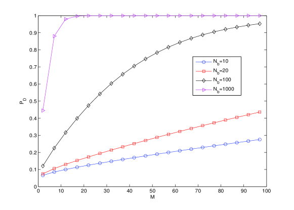
and similarly for PD,ubsubscript𝑃𝐷𝑢𝑏P_{D,ub}, where d1αMNbsubscript𝑑1𝛼𝑀subscript𝑁𝑏d_{1}\triangleq\alpha MN_{b}, d2(1α)MNbsubscript𝑑21𝛼𝑀subscript𝑁𝑏d_{2}\triangleq(1-\alpha)MN_{b}, and αM1/M𝛼subscript𝑀1𝑀\alpha\triangleq M_{1}/M. From (39) and (40) it is clear that for big values of MNb𝑀subscript𝑁𝑏MN_{b}, both μ~~𝜇\tilde{\mu} and σ~~𝜎\tilde{\sigma} are decreasing functions of MNb𝑀subscript𝑁𝑏MN_{b}, and therefore PD,lbsubscript𝑃𝐷𝑙𝑏P_{D,lb} is an increasing function of both M𝑀M and Nbsubscript𝑁𝑏N_{b}. This can be seen also from Figure 1 which illustrates an example of how the performance of the compressive detector changes with the total number of sampling devices M𝑀M and the number of temporal measurements Nbsubscript𝑁𝑏N_{b}. In this example, we set ρ1=ρM1=1subscript𝜌1subscript𝜌subscript𝑀11\rho_{1}=\rho_{M_{1}}=1 and ρN=ρNM2+1=0subscript𝜌𝑁subscript𝜌𝑁subscript𝑀210\rho_{N}=\rho_{N-M_{2}+1}=0 to have PD=PD,lb=PD,ubsubscript𝑃Dsubscript𝑃𝐷𝑙𝑏subscript𝑃𝐷𝑢𝑏P_{\mbox{\scriptsize D}}=P_{D,lb}=P_{D,ub}. Besides, we choose M1=M2=M/2subscript𝑀1subscript𝑀2𝑀2M_{1}=M_{2}=M/2, PFA=0.05subscript𝑃FA0.05P_{\mbox{\scriptsize FA}}=0.05, and σx2=σo2=1superscriptsubscript𝜎𝑥2superscriptsubscript𝜎𝑜21\sigma_{x}^{2}=\sigma_{o}^{2}=1. The probabilities of false alarm and detection are then calculated from (19) and (21).
Refer to caption
Figure 1: Probability of Detection as a function of M𝑀M and Nbsubscript𝑁𝑏N_{b}. Here we have M1=M2=M/2subscript𝑀1subscript𝑀2𝑀2M_{1}=M_{2}=M/2.

Notice that from a practical point of view an important factor which limits utilizing high values of M1subscript𝑀1M_{1} and M2subscript𝑀2M_{2} is the hardware cost and complexity as it is proportional to the number of samplers which is in turn determined by M1subscript𝑀1M_{1} and M2subscript𝑀2M_{2}.

Furthermore, for Nb1much-greater-thansubscript𝑁𝑏1N_{b}\gg 1, one can apply a further approximation on (39) and (40) to obtain

μ~1,~𝜇1\tilde{\mu}\approx 1, (42)

and

σ~2α(1α)NbM.~𝜎2𝛼1𝛼subscript𝑁𝑏𝑀\tilde{\sigma}\approx\sqrt{\frac{2}{\alpha(1-\alpha)N_{b}M}}. (43)

Equation (43) then shows that the performance is optimized for α=0.5𝛼0.5\alpha=0.5, or in other words when we choose M1=M2subscript𝑀1subscript𝑀2M_{1}=M_{2}. This means that when designing a Maximally-Uncorrelated Compressive Detector, the optimum choice is to divide the hardware budget equally between max-energy samplers 𝚽ssubscript𝚽𝑠\mbox{\boldmath$\Phi$\unboldmath}_{s} and min-energy samplers 𝚽osubscript𝚽𝑜\mbox{\boldmath$\Phi$\unboldmath}_{o}.

Refer to caption
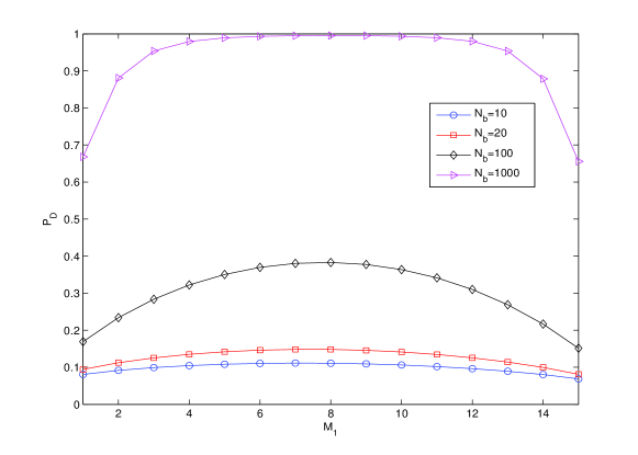
Figure 2: Probability of Detection as a function of M1subscript𝑀1M_{1} and Nbsubscript𝑁𝑏N_{b} for a fixed total number of measurement devices M=16𝑀16M=16.

This can be seen also from Figure 2 which shows that for a fixed number of measurement devices M=16𝑀16M=16, the maximum indeed occurs practically in the middle, which means that the optimum choice is to allocate half of the measurement devices to 𝚽ssubscript𝚽𝑠\mbox{\boldmath$\Phi$\unboldmath}_{s} and the other half to 𝚽osubscript𝚽𝑜\mbox{\boldmath$\Phi$\unboldmath}_{o}.

III-B Fully-Correlated Compressive Detector

In this part, we study the effect of increasing the Signal-to-Noise Ratio (SNR) at the expense of uncorrelatedness of measurement devices. For a certain measurement device, the effective noise energy can be decreased (and therefore the SNR can be increased) by repeating the measurements and averaging over all of them. Collecting the multiple measurements one after the other over time for enhancing the effective SNR is not however a suitable solution here, firstly because the signal itself is random too, and secondly because it increases the latency which is an issue in many applications such as radar or wireless communications due to the relatively quick changes of communication channel characteristics.

However in our proposed measurement framework, improving the effective SNR can be done by employing M1subscript𝑀1M_{1} identical measurement vectors instead of M1×Nsubscript𝑀1𝑁M_{1}\times N measurement matrix 𝚽ssubscript𝚽𝑠\mbox{\boldmath$\Phi$\unboldmath}_{s} in (13) and M2subscript𝑀2M_{2} identical measurement vectors instead of M2×Nsubscript𝑀2𝑁M_{2}\times N measurement matrix 𝚽osubscript𝚽𝑜\mbox{\boldmath$\Phi$\unboldmath}_{o} in (14) and then averaging over all measurements. This will not increase the latency because the identical measurements are taken in parallel. In other words, matrices 𝚽ssubscript𝚽𝑠\mbox{\boldmath$\Phi$\unboldmath}_{s} and 𝚽osubscript𝚽𝑜\mbox{\boldmath$\Phi$\unboldmath}_{o} in (13) and (14) should be respectively redefined as

𝚽s1M𝟏M1,1𝐮1T,subscript𝚽𝑠tensor-product1𝑀subscript1subscript𝑀11superscriptsubscript𝐮1𝑇\mbox{\boldmath$\Phi$\unboldmath}_{s}\triangleq\frac{1}{\sqrt{M}}\mathbf{1}_{M_{1},1}\otimes\mathbf{u}_{1}^{T}, (44)

and

𝚽o1M𝟏M2,1𝐮NT,subscript𝚽𝑜tensor-product1𝑀subscript1subscript𝑀21superscriptsubscript𝐮𝑁𝑇\mbox{\boldmath$\Phi$\unboldmath}_{o}\triangleq\frac{1}{\sqrt{M}}\mathbf{1}_{M_{2},1}\otimes\mathbf{u}_{N}^{T}, (45)

where 𝐮1subscript𝐮1\mathbf{u}_{1} and 𝐮Nsubscript𝐮𝑁\mathbf{u}_{N} are the left singular vectors of 𝐇𝐇\mathbf{H} corresponding to the ρ1subscript𝜌1\rho_{1} and ρNsubscript𝜌𝑁\rho_{N}, respectively. The following theorem is to show the significance of the measurement design in (44) and (45).

Theorem 3.

The measurement sub-matrix 𝚽ssubscript𝚽𝑠\mbox{\boldmath$\Phi$\unboldmath}_{s} in (44) is the solution to the following optimization problem

argmax𝚽𝔼𝐱,𝐰(𝐳s22).subscript𝚽subscript𝔼𝐱𝐰superscriptsubscriptnormsubscript𝐳𝑠22\arg\max_{\mbox{\boldmath$\Phi$\unboldmath}}\mathbb{E}_{\mathbf{x},\mathbf{w}}(\|\mathbf{z}_{s}\|_{2}^{2}). (46)

In other words, the rows of 𝚽ssubscript𝚽𝑠\mbox{\boldmath$\Phi$\unboldmath}_{s} in (44) represent the set of M1subscript𝑀1M_{1} measurement devices that maximize the total energy (or the total variance) in their outputs.

Correspondingly, the measurement sub-matrix 𝚽osubscript𝚽𝑜\mbox{\boldmath$\Phi$\unboldmath}_{o} in (45) is the solution to the following optimization problem

argmin𝚽𝔼𝐱,𝐰(𝐳s22).subscript𝚽subscript𝔼𝐱𝐰superscriptsubscriptnormsubscript𝐳𝑠22\arg\min_{\mbox{\boldmath$\Phi$\unboldmath}}\mathbb{E}_{\mathbf{x},\mathbf{w}}(\|\mathbf{z}_{s}\|_{2}^{2}). (47)

In other words, the rows of 𝚽osubscript𝚽𝑜\mbox{\boldmath$\Phi$\unboldmath}_{o} in (45) represent the set of M2subscript𝑀2M_{2} measurement devices that minimize the total energy (or the total variance) in their outputs.

Proof.

We first notice that

𝔼𝐱,𝐰(𝐳s22)subscript𝔼𝐱𝐰superscriptsubscriptnormsubscript𝐳𝑠22\displaystyle\mathbb{E}_{\mathbf{x},\mathbf{w}}(\|\mathbf{z}_{s}\|_{2}^{2}) =\displaystyle= 𝔼𝐱(𝐱T𝐇T𝚽sT𝚽s𝐇𝐱)+M1σ02Msubscript𝔼𝐱superscript𝐱𝑇superscript𝐇𝑇superscriptsubscript𝚽𝑠𝑇subscript𝚽𝑠𝐇𝐱subscript𝑀1superscriptsubscript𝜎02𝑀\displaystyle\mathbb{E}_{\mathbf{x}}(\mathbf{x}^{T}\mathbf{H}^{T}\mbox{\boldmath$\Phi$\unboldmath}_{s}^{T}\mbox{\boldmath$\Phi$\unboldmath}_{s}\mathbf{H}\mathbf{x})+\frac{M_{1}\sigma_{0}^{2}}{M} (48)
=\displaystyle= σx2trace(𝐇𝐇T𝚽sT𝚽s)+M1σ02Msuperscriptsubscript𝜎𝑥2tracesuperscript𝐇𝐇𝑇superscriptsubscript𝚽𝑠𝑇subscript𝚽𝑠subscript𝑀1superscriptsubscript𝜎02𝑀\displaystyle\sigma_{x}^{2}\mathrm{trace}(\mathbf{H}\mathbf{H}^{T}\mbox{\boldmath$\Phi$\unboldmath}_{s}^{T}\mbox{\boldmath$\Phi$\unboldmath}_{s})+\frac{M_{1}\sigma_{0}^{2}}{M}

Since the second term on the right-hand side of (48) is independent of measurement design, the optimum design for 𝚽ssubscript𝚽𝑠\mbox{\boldmath$\Phi$\unboldmath}_{s} is the one which maximizes the first term. Noticing that 𝐇T𝐇superscript𝐇𝑇𝐇\mathbf{H}^{T}\mathbf{H} and 𝚽sT𝚽ssuperscriptsubscript𝚽𝑠𝑇subscript𝚽𝑠\mbox{\boldmath$\Phi$\unboldmath}_{s}^{T}\mbox{\boldmath$\Phi$\unboldmath}_{s} are both symmetric, from [34, P 11.4.5] we have

trace(𝐇𝐇T𝚽s𝚽sT)i=1M1ρi2λi(𝚽s𝚽sT)tracesuperscript𝐇𝐇𝑇subscript𝚽𝑠superscriptsubscript𝚽𝑠𝑇superscriptsubscript𝑖1subscript𝑀1superscriptsubscript𝜌𝑖2subscript𝜆𝑖subscript𝚽𝑠superscriptsubscript𝚽𝑠𝑇\displaystyle\mathrm{trace}(\mathbf{H}\mathbf{H}^{T}\mbox{\boldmath$\Phi$\unboldmath}_{s}\mbox{\boldmath$\Phi$\unboldmath}_{s}^{T})\leq\sum_{i=1}^{M_{1}}\rho_{i}^{2}\lambda_{i}(\mbox{\boldmath$\Phi$\unboldmath}_{s}\mbox{\boldmath$\Phi$\unboldmath}_{s}^{T}) (49)

Unlike Theorem 1, here we have now no constraint on matrix 𝚽ssubscript𝚽𝑠\mbox{\boldmath$\Phi$\unboldmath}_{s} other than its rows having norm 1/M1𝑀1/\sqrt{M} which means that trace(𝚽s𝚽sT)=i=1M1λi(𝚽s𝚽sT)=M1/Mtracesubscript𝚽𝑠superscriptsubscript𝚽𝑠𝑇superscriptsubscript𝑖1subscript𝑀1subscript𝜆𝑖subscript𝚽𝑠superscriptsubscript𝚽𝑠𝑇subscript𝑀1𝑀\mathrm{trace}(\mbox{\boldmath$\Phi$\unboldmath}_{s}\mbox{\boldmath$\Phi$\unboldmath}_{s}^{T})=\sum_{i=1}^{M_{1}}\lambda_{i}(\mbox{\boldmath$\Phi$\unboldmath}_{s}\mbox{\boldmath$\Phi$\unboldmath}_{s}^{T})=M_{1}/M. Therefore the design of 𝚽ssubscript𝚽𝑠\mbox{\boldmath$\Phi$\unboldmath}_{s} can be done in two steps. In the first step we find the eigenvalues {λi(𝚽s𝚽sT)}i=1M1superscriptsubscriptsubscript𝜆𝑖subscript𝚽𝑠superscriptsubscript𝚽𝑠𝑇𝑖1subscript𝑀1\{\lambda_{i}(\mbox{\boldmath$\Phi$\unboldmath}_{s}\mbox{\boldmath$\Phi$\unboldmath}_{s}^{T})\}_{i=1}^{M_{1}} that maximize the right-hand side of inequality (48). From [40, 4.B.7 and 1.A] the maximum is attained when λ1(𝚽s𝚽sT)=1subscript𝜆1subscript𝚽𝑠superscriptsubscript𝚽𝑠𝑇1\lambda_{1}(\mbox{\boldmath$\Phi$\unboldmath}_{s}\mbox{\boldmath$\Phi$\unboldmath}_{s}^{T})=1 and {λi(𝚽s𝚽sT)}i=2M1=0superscriptsubscriptsubscript𝜆𝑖subscript𝚽𝑠superscriptsubscript𝚽𝑠𝑇𝑖2subscript𝑀10\{\lambda_{i}(\mbox{\boldmath$\Phi$\unboldmath}_{s}\mbox{\boldmath$\Phi$\unboldmath}_{s}^{T})\}_{i=2}^{M_{1}}=0. In the second step we simply employ [34, P 11.4.5] to conclude the proof of (44) being the solution to (46). The proof for (45) is similar. ∎

After designing the samplers as in (44) and (45) and collecting measurement vectors 𝐳s[n]subscript𝐳𝑠delimited-[]𝑛\mathbf{z}_{s}[n] and 𝐳o[n]subscript𝐳𝑜delimited-[]𝑛\mathbf{z}_{o}[n], the effective energy of noise can then be reduced by averaging over all elements of 𝐳s[n]subscript𝐳𝑠delimited-[]𝑛\mathbf{z}_{s}[n] and 𝐳o[n]subscript𝐳𝑜delimited-[]𝑛\mathbf{z}_{o}[n] to obtain

z¯s[n]=1M1𝟏1,M1𝐳s[n],n=1,,Nb,formulae-sequencesubscript¯𝑧𝑠delimited-[]𝑛1subscript𝑀1subscript11subscript𝑀1subscript𝐳𝑠delimited-[]𝑛𝑛1subscript𝑁𝑏\bar{z}_{s}[n]=\frac{1}{M_{1}}\mathbf{1}_{1,M_{1}}\mathbf{z}_{s}[n],~{}n=1,\ldots,N_{b}, (50)

and

z¯o[n]=1M2𝟏1,M2𝐳o[n],n=1,,Nb.formulae-sequencesubscript¯𝑧𝑜delimited-[]𝑛1subscript𝑀2subscript11subscript𝑀2subscript𝐳𝑜delimited-[]𝑛𝑛1subscript𝑁𝑏\bar{z}_{o}[n]=\frac{1}{M_{2}}\mathbf{1}_{1,M_{2}}\mathbf{z}_{o}[n],~{}n=1,\ldots,N_{b}. (51)

In other words, instead of choosing M1subscript𝑀1M_{1} rows of 𝚽ssubscript𝚽𝑠\mbox{\boldmath$\Phi$\unboldmath}_{s} that span the M1subscript𝑀1M_{1}-dimensional subspace along which the energy of signal is maximum as in Section III-A, we choose M1subscript𝑀1M_{1} identical rows for 𝚽ssubscript𝚽𝑠\mbox{\boldmath$\Phi$\unboldmath}_{s} each as the 111-dimensional subspace along which the energy of signal is maximum, and then decrease the noise power (and therefore increase the effective SNR) by averaging over all M1subscript𝑀1M_{1} measurements. Similarly, for 𝚽osubscript𝚽𝑜\mbox{\boldmath$\Phi$\unboldmath}_{o}, instead of choosing its M2subscript𝑀2M_{2} rows that span the M2subscript𝑀2M_{2}-dimensional subspace along which the energy of signal is minimum as in Section III-A, we choose M2subscript𝑀2M_{2} identical rows for 𝚽osubscript𝚽𝑜\mbox{\boldmath$\Phi$\unboldmath}_{o} each as the 111-dimensional subspace along which the energy of signal is minimum, and thus decrease the noise energy (and therefore increase the effective SNR) by averaging over all M2subscript𝑀2M_{2} measurements.

The following theorem introduces the test for performing (8) based on measurement design in (44) and (45).

Theorem 4.

Consider the following test for compressive detection of subspace signal 𝐇𝐱𝐇𝐱\mathbf{H}\mathbf{x}

𝒯=M1n=1Nb|z¯s[n]|2M2n=1Nb|z¯o[n]|201γ𝒯subscript𝑀1superscriptsubscript𝑛1subscript𝑁𝑏superscriptsubscript¯𝑧𝑠delimited-[]𝑛2subscript𝑀2superscriptsubscript𝑛1subscript𝑁𝑏superscriptsubscript¯𝑧𝑜delimited-[]𝑛2subscript1subscript0greater-than-or-less-than𝛾\mathcal{T}=\frac{M_{1}\sum\limits_{n=1}^{N_{b}}|\bar{z}_{s}[n]|^{2}}{M_{2}\sum\limits_{n=1}^{N_{b}}|\bar{z}_{o}[n]|^{2}}\overset{\mathcal{H}_{1}}{\underset{\mathcal{H}_{0}}{\gtrless}}\gamma (52)

The probability of false alarm PFAsubscript𝑃FAP_{\mbox{\scriptsize FA}} and the probability of detection PDsubscript𝑃DP_{\mbox{\scriptsize D}} are then expressed as

PFA=F(Nb,Nb)(γ),subscript𝑃FAsubscript𝐹subscript𝑁𝑏subscript𝑁𝑏𝛾P_{\mbox{\scriptsize FA}}=\mathbb{Q}_{F(N_{b},N_{b})}(\gamma), (53)

and

PD=F(Nb,Nb)(σ02+M2σx2ρN2σ02+M1σx2ρ12γ).subscript𝑃Dsubscript𝐹subscript𝑁𝑏subscript𝑁𝑏superscriptsubscript𝜎02subscript𝑀2superscriptsubscript𝜎𝑥2superscriptsubscript𝜌𝑁2superscriptsubscript𝜎02subscript𝑀1superscriptsubscript𝜎𝑥2superscriptsubscript𝜌12𝛾P_{\mbox{\scriptsize D}}=\mathbb{Q}_{F(N_{b},N_{b})}\Big{(}\frac{\sigma_{0}^{2}+M_{2}\sigma_{x}^{2}\rho_{N}^{2}}{\sigma_{0}^{2}+M_{1}\sigma_{x}^{2}\rho_{1}^{2}}\gamma\Big{)}. (54)
Proof.

To derive the probability of false alarm PFAsubscript𝑃FAP_{\mbox{\scriptsize FA}} and the probability of detection PDsubscript𝑃DP_{\mbox{\scriptsize D}}, we first notice that if the Gaussian noise is i.i.d, then it is easy to observe that the distribution of z¯o[n]subscript¯𝑧𝑜delimited-[]𝑛\bar{z}_{o}[n] is

z¯o[n]{𝒩(0,σ02MM2)under0,𝒩(0,σ02MM2+1Mσx2ρN2)under1.similar-tosubscript¯𝑧𝑜delimited-[]𝑛cases𝒩0superscriptsubscript𝜎02𝑀subscript𝑀2undersubscript0missing-subexpressionmissing-subexpression𝒩0superscriptsubscript𝜎02𝑀subscript𝑀21𝑀superscriptsubscript𝜎𝑥2superscriptsubscript𝜌𝑁2undersubscript1\bar{z}_{o}[n]\sim\left\{\begin{array}[]{ll}\mathcal{N}(0,\frac{\sigma_{0}^{2}}{MM_{2}})&\mathrm{under~{}}\mathcal{H}_{0},\\ \\ \mathcal{N}(0,\frac{\sigma_{0}^{2}}{MM_{2}}+\frac{1}{M}\sigma_{x}^{2}\rho_{N}^{2})&\mathrm{under~{}}\mathcal{H}_{1}.\end{array}\right. (55)

Similarly, the distribution of z¯s[n]subscript¯𝑧𝑠delimited-[]𝑛\bar{z}_{s}[n] is

z¯s[n]{𝒩(0,σ02MM1)under0,𝒩(0,σ02MM1+1Mσx2ρ12)under1,similar-tosubscript¯𝑧𝑠delimited-[]𝑛cases𝒩0superscriptsubscript𝜎02𝑀subscript𝑀1undersubscript0missing-subexpressionmissing-subexpression𝒩0superscriptsubscript𝜎02𝑀subscript𝑀11𝑀superscriptsubscript𝜎𝑥2superscriptsubscript𝜌12undersubscript1\bar{z}_{s}[n]\sim\left\{\begin{array}[]{ll}\mathcal{N}(0,\frac{\sigma_{0}^{2}}{MM_{1}})&\mathrm{under~{}}\mathcal{H}_{0},\\ \\ \mathcal{N}(0,\frac{\sigma_{0}^{2}}{MM_{1}}+\frac{1}{M}\sigma_{x}^{2}\rho_{1}^{2})&\mathrm{under~{}}\mathcal{H}_{1},\end{array}\right. (56)

Then by following steps similar to those in Theorem 2, (53) and (54) are concluded. ∎

The Fully-Correlated Compressive Detector of (44) and (45) whose probabilities of false alarm and detection were derived in Theorem 4 is optimum in terms of providing the largest difference between the expected energy of its two set of samplers. However as discussed earlier, a major measure of interest in statistical hypothesis testing is the power of the test. The following corollary discusses the optimality of the proposed Fully-Correlated Compressive design and detector in terms of the power of the test.

Corollary 2.

Among all fully-correlated measurement designs of the form

𝚽s1M𝟏M1,1𝐭1T,subscript𝚽𝑠tensor-product1𝑀subscript1subscript𝑀11superscriptsubscript𝐭1𝑇\mbox{\boldmath$\Phi$\unboldmath}_{s}\triangleq\frac{1}{\sqrt{M}}\mathbf{1}_{M_{1},1}\otimes\mathbf{t}_{1}^{T}, (57)

and

𝚽o1M𝟏M2,1𝐭2T,subscript𝚽𝑜tensor-product1𝑀subscript1subscript𝑀21superscriptsubscript𝐭2𝑇\mbox{\boldmath$\Phi$\unboldmath}_{o}\triangleq\frac{1}{\sqrt{M}}\mathbf{1}_{M_{2},1}\otimes\mathbf{t}_{2}^{T}, (58)

with 𝐭12=𝐭22=1subscriptnormsubscript𝐭12subscriptnormsubscript𝐭221\|\mathbf{t}_{1}\|_{2}=\|\mathbf{t}_{2}\|_{2}=1 and 𝐭1T𝐭2=0superscriptsubscript𝐭1𝑇subscript𝐭20\mathbf{t}_{1}^{T}\mathbf{t}_{2}=0, the one proposed in (44) and (45) delivers the highest PDsubscript𝑃DP_{\mbox{\scriptsize D}} for a fixed PFAsubscript𝑃FAP_{\mbox{\scriptsize FA}} for performing the test given in (52).

Proof.

By taking steps similar to the proof of Theorem 4, the probability of false alarm can be derived as PFA=F(Nb,Nb)(γ)subscript𝑃FAsubscript𝐹subscript𝑁𝑏subscript𝑁𝑏𝛾P_{\mbox{\scriptsize FA}}=\mathbb{Q}_{F(N_{b},N_{b})}(\gamma). Therefore, for a given PFAsubscript𝑃FAP_{\mbox{\scriptsize FA}}, M1subscript𝑀1M_{1}, M2subscript𝑀2M_{2}, and Nbsubscript𝑁𝑏N_{b}, we can write

PD=F(Nb,Nb)(σ02+M2σx2𝐭2T𝐇𝐇T𝐭2σ02+M1σx2𝐭1T𝐇𝐇T𝐭1F(Nb,Nb)1(PFA)).subscript𝑃Dsubscript𝐹subscript𝑁𝑏subscript𝑁𝑏superscriptsubscript𝜎02subscript𝑀2superscriptsubscript𝜎𝑥2superscriptsubscript𝐭2𝑇superscript𝐇𝐇𝑇subscript𝐭2superscriptsubscript𝜎02subscript𝑀1superscriptsubscript𝜎𝑥2superscriptsubscript𝐭1𝑇superscript𝐇𝐇𝑇subscript𝐭1superscriptsubscript𝐹subscript𝑁𝑏subscript𝑁𝑏1subscript𝑃FAP_{\mbox{\scriptsize D}}=\mathbb{Q}_{F(N_{b},N_{b})}\Big{(}\frac{\sigma_{0}^{2}+M_{2}\sigma_{x}^{2}\mathbf{t}_{2}^{T}\mathbf{H}\mathbf{H}^{T}\mathbf{t}_{2}}{\sigma_{0}^{2}+M_{1}\sigma_{x}^{2}\mathbf{t}_{1}^{T}\mathbf{H}\mathbf{H}^{T}\mathbf{t}_{1}}\mathbb{Q}_{F(N_{b},N_{b})}^{-1}(P_{\mbox{\scriptsize FA}})\Big{)}. (59)

From (59), it is clear that the most powerful design is the one that minimizes σ02+M2σx2𝐭2T𝐇𝐇T𝐭2σ02+M1σx2𝐭1T𝐇𝐇T𝐭1superscriptsubscript𝜎02subscript𝑀2superscriptsubscript𝜎𝑥2superscriptsubscript𝐭2𝑇superscript𝐇𝐇𝑇subscript𝐭2superscriptsubscript𝜎02subscript𝑀1superscriptsubscript𝜎𝑥2superscriptsubscript𝐭1𝑇superscript𝐇𝐇𝑇subscript𝐭1\frac{\sigma_{0}^{2}+M_{2}\sigma_{x}^{2}\mathbf{t}_{2}^{T}\mathbf{H}\mathbf{H}^{T}\mathbf{t}_{2}}{\sigma_{0}^{2}+M_{1}\sigma_{x}^{2}\mathbf{t}_{1}^{T}\mathbf{H}\mathbf{H}^{T}\mathbf{t}_{1}}, which in turn is the one that minimizes 𝐭2T𝐇𝐇T𝐭2superscriptsubscript𝐭2𝑇superscript𝐇𝐇𝑇subscript𝐭2\mathbf{t}_{2}^{T}\mathbf{H}\mathbf{H}^{T}\mathbf{t}_{2} and maximizes 𝐭1T𝐇𝐇T𝐭1superscriptsubscript𝐭1𝑇superscript𝐇𝐇𝑇subscript𝐭1\mathbf{t}_{1}^{T}\mathbf{H}\mathbf{H}^{T}\mathbf{t}_{1}. Then by employing the Rayleigh-Ritz theorem [36, Chapter 8] it can be easily proven that the optimum design is 𝐭1=𝐮1subscript𝐭1subscript𝐮1\mathbf{t}_{1}=\mathbf{u}_{1} and 𝐭2=𝐮Nsubscript𝐭2subscript𝐮𝑁\mathbf{t}_{2}=\mathbf{u}_{N}. ∎

Again, similar to the Maximally-Uncorrelated case, Theorem 3 and Corollary 2 result in identical solution although they are trying to optimize different cost functions, which is because the proposed detector is in fact an F𝐹F-test detector working based on the difference between the variances of the two sets of measurements.

The performance of Fully Correlated Detector has a clear connection to the way we choose the number of samplers. The following Corollary discusses this.

Corollary 3.

For a given number of samplers M𝑀M and probability of false alarm PFAsubscript𝑃FAP_{\mbox{\scriptsize FA}}, the performance of the detector PDsubscript𝑃DP_{\mbox{\scriptsize D}} is maximized when M2=1subscript𝑀21M_{2}=1 and M1=M1subscript𝑀1𝑀1M_{1}=M-1.

Proof.

First, we notice from (53) that the threshold level γ𝛾\gamma is independent of the choice of M1subscript𝑀1M_{1} and M2subscript𝑀2M_{2}. Then from (54) it is clear that PDsubscript𝑃DP_{\mbox{\scriptsize D}} achieves its maximum value when M2subscript𝑀2M_{2} reaches its minimum value and M1subscript𝑀1M_{1} reaches its maximum value. ∎

The above Corollary asserts that in the case of Fully-Correlated Detector, for a fixed hardware budget, in terms of the total number of samplers M=M1+M2𝑀subscript𝑀1subscript𝑀2M=M_{1}+M_{2}, the best performance, in terms of PDsubscript𝑃DP_{\mbox{\scriptsize D}}, is obtained if we employ just one sampler for 𝚽osubscript𝚽𝑜\mbox{\boldmath$\Phi$\unboldmath}_{o} and spend the rest of the hardware budget on 𝚽ssubscript𝚽𝑠\mbox{\boldmath$\Phi$\unboldmath}_{s}. Besides, by putting the optimum values M2=1subscript𝑀21M_{2}=1 and M1=M1subscript𝑀1𝑀1M_{1}=M-1 in (54) it is clear that the performance enhances as the total number of measurement devices M𝑀M grows.

Refer to caption
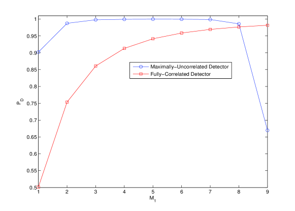
Figure 3: Probability of Detection as a function of M1subscript𝑀1M_{1} for the two detectors introduced in Sections III-A and III-B. The total number of samplers is M=10𝑀10M=10, the Signal-to-Noise Ratio is σx2σ02=0dBsuperscriptsubscript𝜎𝑥2superscriptsubscript𝜎020dB\frac{\sigma_{x}^{2}}{\sigma_{0}^{2}}=0\mathrm{dB} and the largest and smallest eigenvalues of 𝐇𝐇Tsuperscript𝐇𝐇𝑇\mathbf{H}\mathbf{H}^{T} are ρ12=10superscriptsubscript𝜌1210\rho_{1}^{2}=10 and ρN2superscriptsubscript𝜌𝑁2\rho_{N}^{2}=0, respectively. The Probability of False Alarm is PFA=0.01subscript𝑃FA0.01P_{\mbox{\scriptsize FA}}=0.01 and the number of temporal measurements is Nb=5subscript𝑁𝑏5N_{b}=5.

Figure 3 demonstrates an example of how the probability of detection for Fully-Correlated detector changes with the number of maximum energy samplers M1subscript𝑀1M_{1}. The performance curve of the Maximally-Uncorrelated case is also shown for comparison. As it can be observed, while the performance of Fully-Correlated detector clearly enhances with increasing M1subscript𝑀1M_{1}, the performance of Maximally-Uncorrelated Detector does not show such a monotonic relationship. The best performance of the Maximally-Uncorrelated Detector here is achieved for M1=M2=5subscript𝑀1subscript𝑀25M_{1}=M_{2}=5. The probabilities of detection of the two detectors here have been calculated from (54) and (21). The parameters of the Maximally-Uncorrelated detector has been chosen such that PD=PD,lb=PD,ubsubscript𝑃Dsubscript𝑃𝐷𝑙𝑏subscript𝑃𝐷𝑢𝑏P_{\mbox{\scriptsize D}}=P_{D,lb}=P_{D,ub}.

Remark 4: Comparing (46) and (47) to (15) and (16) it may seem that the performance of the Fully-Correlated detector is always superior to the Maximally-Uncorrelated detector as the optimizations in (46) and (47) are unconstrained compared to the optimizations in (15) and (16) which are constrained. However, we should notice that this is not always the case as Maximally-Uncorrelated detector provides a higher diversity in its collected samples, which is reflected by the higher degrees of freedom in (19), (21) and (22) compared to (53) and (54). For example consider the case when 𝐱[n]𝐱delimited-[]𝑛\mathbf{x}[n] is present but lies orthogonal to the strongest right singular vector of 𝐇𝐇\mathbf{H}. Then for the Fully-Correlated samplers the energy of samples collected by all of the M1subscript𝑀1M_{1} samplers 𝚽ssubscript𝚽𝑠\mbox{\boldmath$\Phi$\unboldmath}_{s} includes only the energy of noise while for the Maximally-Uncorrelated Compressive Detector only the output energy of the first max-energy sampler is equivalent to the noise energy and the output of the rest of M11subscript𝑀11M_{1}-1 samplers include both the signal and the noise energy. This can also be seen from the example of Figure 3 where the best performance of the Fully-Correlated detector occurring at M1=M1=9subscript𝑀1𝑀19M_{1}=M-1=9 is inferior to the best performance of Maximally-Uncorrelated detector occurring at M1=M/2=5subscript𝑀1𝑀25M_{1}=M/2=5.

III-C Special Case of Known Noise Variance

As discussed earlier in this Section, the idea of having two sets of measurement devices 𝚽ssubscript𝚽𝑠\mbox{\boldmath$\Phi$\unboldmath}_{s} and 𝚽osubscript𝚽𝑜\mbox{\boldmath$\Phi$\unboldmath}_{o} is to have two sets of measurements with maximum difference in their variances when the signal truly exists and equivalent variances when the signal does not exist and then making decision about the existence of signal based on this difference. However, if the variance of noise is known, we can simplify the proposed design by discarding 𝚽osubscript𝚽𝑜\mbox{\boldmath$\Phi$\unboldmath}_{o} as we can simply compare the variance of the output of 𝚽ssubscript𝚽𝑠\mbox{\boldmath$\Phi$\unboldmath}_{s} to the known noise variance. In other words, we can employ only M1subscript𝑀1M_{1} measurement devices determined by the rows of 𝚽ssubscript𝚽𝑠\mbox{\boldmath$\Phi$\unboldmath}_{s} and then compare the power of measurements taken by them to the power of noise: if they are almost the same then we decide that no signal exists, if not then we decide that signal exists.

Similar to the two detectors proposed in sections III-A and III-B, we can have two detectors when the noise variance is known. The following two propositions express these two detectors and their performances. We remark that since 𝚽osubscript𝚽𝑜\mbox{\boldmath$\Phi$\unboldmath}_{o} is discarded when noise variance is known, we will have M2=0subscript𝑀20M_{2}=0 and therefore the whole number of measurement devices is M=M1𝑀subscript𝑀1M=M_{1}.

Proposition 1.

If we design the measurement matrix according to (13), then in the case of known σ02superscriptsubscript𝜎02\sigma_{0}^{2}, the test in (18) can be replaced by

𝒯=n=1Nb𝐳s[n]T𝐳s[n]σ02/M101γ.𝒯superscriptsubscript𝑛1subscript𝑁𝑏subscript𝐳𝑠superscriptdelimited-[]𝑛𝑇subscript𝐳𝑠delimited-[]𝑛superscriptsubscript𝜎02subscript𝑀1subscript1subscript0greater-than-or-less-than𝛾\mathcal{T}=\frac{\sum\limits_{n=1}^{N_{b}}\mathbf{z}_{s}[n]^{T}\mathbf{z}_{s}[n]}{\sigma_{0}^{2}/M_{1}}\overset{\mathcal{H}_{1}}{\underset{\mathcal{H}_{0}}{\gtrless}}\gamma. (60)

The Probability of False Alarm, PFAsubscript𝑃FAP_{\mbox{\scriptsize FA}}, for this test is computed as

PFA=χ2(M1Nb)(γ),subscript𝑃FAsubscriptsuperscript𝜒2subscript𝑀1subscript𝑁𝑏𝛾P_{\mbox{\scriptsize FA}}=\mathbb{Q}_{\chi^{2}(M_{1}N_{b})}(\gamma), (61)

and the Probability of Detection, PDsubscript𝑃DP_{\mbox{\scriptsize D}}, is bounded as

PD,lbPDPD,ubsubscript𝑃𝐷𝑙𝑏subscript𝑃Dsubscript𝑃𝐷𝑢𝑏P_{D,lb}\leq P_{\mbox{\scriptsize D}}\leq P_{D,ub} (62)

where PD,lbsubscript𝑃𝐷𝑙𝑏P_{D,lb} and PD,ubsubscript𝑃𝐷𝑢𝑏P_{D,ub} are, respectively, the lower bound and the upper bound for the probability of detection which will take the following formulas

PD,lb=χ2(M1Nb)(ηlbγ),subscript𝑃𝐷𝑙𝑏subscriptsuperscript𝜒2subscript𝑀1subscript𝑁𝑏superscriptsubscript𝜂𝑙𝑏𝛾P_{D,lb}=\mathbb{Q}_{\chi^{2}(M_{1}N_{b})}({\eta_{lb}^{\prime}}\gamma), (63)

and

PD,ub=χ2(M1Nb)(ηubγ),subscript𝑃𝐷𝑢𝑏subscriptsuperscript𝜒2subscript𝑀1subscript𝑁𝑏superscriptsubscript𝜂𝑢𝑏𝛾P_{D,ub}=\mathbb{Q}_{\chi^{2}(M_{1}N_{b})}({\eta_{ub}^{\prime}}\gamma), (64)

where ηlbσ02σ02+σx2ρM12superscriptsubscript𝜂𝑙𝑏superscriptsubscript𝜎02superscriptsubscript𝜎02superscriptsubscript𝜎𝑥2superscriptsubscript𝜌subscript𝑀12\eta_{lb}^{\prime}\triangleq\frac{\sigma_{0}^{2}}{\sigma_{0}^{2}+\sigma_{x}^{2}\rho_{M_{1}}^{2}}, ηubσ02σ02+σx2ρ12superscriptsubscript𝜂𝑢𝑏superscriptsubscript𝜎02superscriptsubscript𝜎02superscriptsubscript𝜎𝑥2superscriptsubscript𝜌12\eta_{ub}^{\prime}\triangleq\frac{\sigma_{0}^{2}}{\sigma_{0}^{2}+\sigma_{x}^{2}\rho_{1}^{2}}, and χ2(d)(x)subscriptsuperscript𝜒2𝑑𝑥\mathbb{Q}_{\chi^{2}(d)}(x) is the tail probability of the chi-squared distribution with parameter (degree of freedom) d𝑑d at point x𝑥x.

Proposition 2.

If we design the measurement matrix according to (44), then in the case of known σ02superscriptsubscript𝜎02\sigma_{0}^{2}, the test in (52) can be replaced by

𝒯=n=1Nb|z¯s[n]|2σ02/M1201γ𝒯superscriptsubscript𝑛1subscript𝑁𝑏superscriptsubscript¯𝑧𝑠delimited-[]𝑛2superscriptsubscript𝜎02superscriptsubscript𝑀12subscript1subscript0greater-than-or-less-than𝛾\mathcal{T}=\frac{\sum\limits_{n=1}^{N_{b}}|\bar{z}_{s}[n]|^{2}}{\sigma_{0}^{2}/M_{1}^{2}}\overset{\mathcal{H}_{1}}{\underset{\mathcal{H}_{0}}{\gtrless}}\gamma (65)

The Probability of False Alarm, PFAsubscript𝑃FAP_{\mbox{\scriptsize FA}}, for this test is

PFA=χ2(Nb)(γ),subscript𝑃FAsubscriptsuperscript𝜒2subscript𝑁𝑏𝛾P_{\mbox{\scriptsize FA}}=\mathbb{Q}_{\chi^{2}(N_{b})}(\gamma), (66)

and

PD=χ2(Nb)(σ02σ02+M1σx2ρ12γ).subscript𝑃Dsubscriptsuperscript𝜒2subscript𝑁𝑏superscriptsubscript𝜎02superscriptsubscript𝜎02subscript𝑀1superscriptsubscript𝜎𝑥2superscriptsubscript𝜌12𝛾P_{\mbox{\scriptsize D}}=\mathbb{Q}_{\chi^{2}(N_{b})}\Big{(}\frac{\sigma_{0}^{2}}{\sigma_{0}^{2}+M_{1}\sigma_{x}^{2}\rho_{1}^{2}}\gamma\Big{)}. (67)

III-D Compressive Detection in Presence of Known Subspace Interference

Extending the above results to the subspace interference case is straightforward and is similar to the same scenario for classical uncompressive detection of deterministic subspace signals in presence of interference in [41]. Suppose that the subspace signal model in (1) is replaced by

𝐬[n]=𝐇𝐱[n]+𝐆𝐭[n],𝐬delimited-[]𝑛𝐇𝐱delimited-[]𝑛𝐆𝐭delimited-[]𝑛\mathbf{s}[n]=\mathbf{H}\mathbf{x}[n]+\mathbf{G}\mathbf{t}[n], (68)

where 𝐆𝐆\mathbf{G} is an N×K𝑁superscript𝐾N\times K^{\prime} matrix and the second term on the right-hand side of (68) represents the subspace interference. If 𝐬[n]𝐬delimited-[]𝑛\mathbf{s}[n] were available, the interference could be cancelled by left multiplying (68) by matrix 𝐏𝐆=𝐈𝐆(𝐆T𝐆)1𝐆Tsuperscriptsubscript𝐏𝐆perpendicular-to𝐈𝐆superscriptsuperscript𝐆𝑇𝐆1superscript𝐆𝑇\mathbf{P}_{\mathbf{G}}^{\perp}=\mathbf{I}-\mathbf{G}(\mathbf{G}^{T}\mathbf{G})^{-1}\mathbf{G}^{T} to obtain

𝐏𝐆𝐬[n]=𝐏𝐆𝐇𝐱[n].superscriptsubscript𝐏𝐆perpendicular-to𝐬delimited-[]𝑛superscriptsubscript𝐏𝐆perpendicular-to𝐇𝐱delimited-[]𝑛\mathbf{P}_{\mathbf{G}}^{\perp}\mathbf{s}[n]=\mathbf{P}_{\mathbf{G}}^{\perp}\mathbf{H}\mathbf{x}[n]. (69)

Comparing (69) to (1), it can be easily deduced that in this scenario to design the measurement vectors, i.e., rows of 𝚽𝚽\Phi, the left-singular vectors of matrix 𝐇𝐇\mathbf{H} in the interference-free scenario in (13) and (14) must be replaced by left-singular vectors of matrix 𝐏𝐆𝐇superscriptsubscript𝐏𝐆perpendicular-to𝐇\mathbf{P}_{\mathbf{G}}^{\perp}\mathbf{H} right-multiplied by matrix 𝐏𝐆superscriptsubscript𝐏𝐆perpendicular-to\mathbf{P}_{\mathbf{G}}^{\perp}. Otherwise, all the detector developments are similar to the previous subsections.

IV Compressive Detector with Non-Ideal Measurements

In this section we investigate the case when due to the lack of complete knowledge about the subspace or due to the limitations in designing hardware with infinite precision, the measurement vectors do not exactly match the singular vectors of matrix 𝐇𝐇\mathbf{H}. We consider two models for describing this uncertainty. The first model, defines the finite precision using additional observation noise. The second model, on the other hand, chooses the measurement vector from a set of realizable measurement vectors (hardware) which are approximations (or quantized versions) of infinite-precision real-valued singular vectors.

IV-A Compressive Detection with Imprecise Measurements

In this section we analyze the detector when the measurement device is not precise. This imprecision in measurements can be modeled as [42]

𝐳~[n]=𝐳[n]+δ1/2ϵ[n],~𝐳delimited-[]𝑛𝐳delimited-[]𝑛superscript𝛿12bold-italic-ϵdelimited-[]𝑛\tilde{\mathbf{z}}[n]=\mathbf{z}[n]+\delta^{-1/2}\mbox{\boldmath$\epsilon$\unboldmath}[n], (70)

where 𝐳~[n]~𝐳delimited-[]𝑛\tilde{\mathbf{z}}[n] denotes the imprecise compressive measurements, 𝐳[n]𝐳delimited-[]𝑛\mathbf{z}[n] denotes the basic measurements as introduced in Section II, ϵ[n]𝒩(𝟎M,1,𝐈M)similar-tobold-italic-ϵdelimited-[]𝑛𝒩subscript0𝑀1subscript𝐈𝑀\mbox{\boldmath$\epsilon$\unboldmath}[n]\sim\mathcal{N}(\mathbf{0}_{M,1},\mathbf{I}_{M}), and δ𝛿\delta represents the precision of measurements. Thus the imprecision is here modeled through additional observation or measurement noise, as in [42].

Now, if we replace 𝐳s[n]subscript𝐳𝑠delimited-[]𝑛\mathbf{z}_{s}[n] and 𝐳o[n]subscript𝐳𝑜delimited-[]𝑛\mathbf{z}_{o}[n] in the test statistic (18) of Maximally-Uncorrelated detector by 𝐳~s[n]𝐳~[n]|1:M1subscript~𝐳𝑠delimited-[]𝑛evaluated-at~𝐳delimited-[]𝑛:1subscript𝑀1\tilde{\mathbf{z}}_{s}[n]\triangleq\tilde{\mathbf{z}}[n]\Big{|}_{1:M_{1}} and 𝐳~o[n]𝐳~[n]|M1+1:Msubscript~𝐳𝑜delimited-[]𝑛evaluated-at~𝐳delimited-[]𝑛:subscript𝑀11𝑀\tilde{\mathbf{z}}_{o}[n]\triangleq\tilde{\mathbf{z}}[n]\Big{|}_{M_{1}+1:M}, respectively, then it can be easily verified that the probability of false alarm will be the same as in (19), but the lower and upper bounds of probability of detection in (21) and (22) will be replaced by

PD,lb=F(M1Nb,M2Nb)(σ02+σx2ρNM2+12+Mδ1σ02+σx2ρM12+Mδ1γ),subscript𝑃𝐷𝑙𝑏subscript𝐹subscript𝑀1subscript𝑁𝑏subscript𝑀2subscript𝑁𝑏superscriptsubscript𝜎02superscriptsubscript𝜎𝑥2superscriptsubscript𝜌𝑁subscript𝑀212𝑀superscript𝛿1superscriptsubscript𝜎02superscriptsubscript𝜎𝑥2superscriptsubscript𝜌subscript𝑀12𝑀superscript𝛿1𝛾P_{D,lb}=\mathbb{Q}_{F(M_{1}N_{b},M_{2}N_{b})}({\frac{\sigma_{0}^{2}+\sigma_{x}^{2}\rho_{N-M_{2}+1}^{2}+M\delta^{-1}}{\sigma_{0}^{2}+\sigma_{x}^{2}\rho_{M_{1}}^{2}+M\delta^{-1}}\gamma}), (71)

and

PD,ub=F(M1Nb,M2Nb)(σ02+σx2ρN2+Mδ1σ02+σx2ρ12+Mδ1γ),subscript𝑃𝐷𝑢𝑏subscript𝐹subscript𝑀1subscript𝑁𝑏subscript𝑀2subscript𝑁𝑏superscriptsubscript𝜎02superscriptsubscript𝜎𝑥2superscriptsubscript𝜌𝑁2𝑀superscript𝛿1superscriptsubscript𝜎02superscriptsubscript𝜎𝑥2superscriptsubscript𝜌12𝑀superscript𝛿1𝛾P_{D,ub}=\mathbb{Q}_{F(M_{1}N_{b},M_{2}N_{b})}({\frac{\sigma_{0}^{2}+\sigma_{x}^{2}\rho_{N}^{2}+M\delta^{-1}}{\sigma_{0}^{2}+\sigma_{x}^{2}\rho_{1}^{2}+M\delta^{-1}}\gamma}), (72)

respectively. Comparing (71) and (72) with (21) and (22), it is clear that the performance degrades as the precision of measurement devices δ𝛿\delta decreases. This can be however compensated by improving the precision through employing several, say L𝐿L, identical measurement devices instead of each device and then averaging over all measurements. In other words, instead of M𝑀M measurement devices, we employ ML𝑀𝐿ML to improve the performance. We call L𝐿L the hardware budget factor as it indicates the number of measurement devices that we employ.

In this case, the probability of false alarm will be still expressed as in (19) while the lower and upper bounds for probability of detection are modified as

PD,lb=F(M1Nb,M2Nb)(σ02+Lσx2ρNM2+12+Mδ1σ02+Lσx2ρM12+Mδ1γ),subscript𝑃𝐷𝑙𝑏subscript𝐹subscript𝑀1subscript𝑁𝑏subscript𝑀2subscript𝑁𝑏superscriptsubscript𝜎02𝐿superscriptsubscript𝜎𝑥2superscriptsubscript𝜌𝑁subscript𝑀212𝑀superscript𝛿1superscriptsubscript𝜎02𝐿superscriptsubscript𝜎𝑥2superscriptsubscript𝜌subscript𝑀12𝑀superscript𝛿1𝛾P_{D,lb}=\mathbb{Q}_{F(M_{1}N_{b},M_{2}N_{b})}({\frac{\sigma_{0}^{2}+L\sigma_{x}^{2}\rho_{N-M_{2}+1}^{2}+M\delta^{-1}}{\sigma_{0}^{2}+L\sigma_{x}^{2}\rho_{M_{1}}^{2}+M\delta^{-1}}\gamma}), (73)

and

PD,ub=F(M1Nb,M2Nb)(σ02+Lσx2ρN2+Mδ1σ02+Lσx2ρ12+Mδ1γ),subscript𝑃𝐷𝑢𝑏subscript𝐹subscript𝑀1subscript𝑁𝑏subscript𝑀2subscript𝑁𝑏superscriptsubscript𝜎02𝐿superscriptsubscript𝜎𝑥2superscriptsubscript𝜌𝑁2𝑀superscript𝛿1superscriptsubscript𝜎02𝐿superscriptsubscript𝜎𝑥2superscriptsubscript𝜌12𝑀superscript𝛿1𝛾P_{D,ub}=\mathbb{Q}_{F(M_{1}N_{b},M_{2}N_{b})}({\frac{\sigma_{0}^{2}+L\sigma_{x}^{2}\rho_{N}^{2}+M\delta^{-1}}{\sigma_{0}^{2}+L\sigma_{x}^{2}\rho_{1}^{2}+M\delta^{-1}}\gamma}), (74)

Comparing (73) and (74) with (21) and (22), the hardware budget factor L𝐿L for achieving a performance similar or better than the infinite precision case of δ1=0superscript𝛿10\delta^{-1}=0 is obtained as

L1+Mδσ02.𝐿1𝑀𝛿superscriptsubscript𝜎02L\geq 1+\frac{M}{\delta\sigma_{0}^{2}}. (75)

IV-B Compressive Detection Using a Fixed Set of Measurement Vectors

The second model in this section for modeling non-ideal measurement devices is formulated as choosing the measurement vectors from a fixed set of unit-norm orthogonal vectors whose members are not necessarily singular vectors of the system matrix 𝐇𝐇\mathbf{H}. These vectors can be hardware-realizable approximation of the singular vectors, e.g. quantized versions of them, or simple down-samplers. Assume that M=M1+M2𝑀subscript𝑀1subscript𝑀2M=M_{1}+M_{2} measurement vectors should be chosen out of RM𝑅𝑀R\geq M uncorrelated columns of N×R𝑁𝑅N\times R matrix 𝚿=[𝝍1,𝝍2,,𝝍R]𝚿subscript𝝍1subscript𝝍2subscript𝝍𝑅\mbox{\boldmath$\Psi$\unboldmath}=[\mbox{\boldmath$\psi$\unboldmath}_{1},\mbox{\boldmath$\psi$\unboldmath}_{2},\ldots,\mbox{\boldmath$\psi$\unboldmath}_{R}] (notice that M𝚿T𝚿=𝐈R𝑀superscript𝚿𝑇𝚿subscript𝐈𝑅M\mbox{\boldmath$\Psi$\unboldmath}^{T}\mbox{\boldmath$\Psi$\unboldmath}=\mathbf{I}_{R}). The rows of 𝚽ssubscript𝚽𝑠\mbox{\boldmath$\Phi$\unboldmath}_{s} and 𝚽osubscript𝚽𝑜\mbox{\boldmath$\Phi$\unboldmath}_{o} then have to be chosen from the columns of 𝚿𝚿\Psi.

The optimum 𝚽ssubscript𝚽𝑠\mbox{\boldmath$\Phi$\unboldmath}_{s} is the one that maximizes the energy of its output. If we want to follow the Maximally-Uncorrelated design of Section III-A, then the rows of 𝚽ssubscript𝚽𝑠\mbox{\boldmath$\Phi$\unboldmath}_{s} are the M1subscript𝑀1M_{1} columns of 𝚿𝚿\Psi for which 𝚽s𝐇Fsubscriptnormsubscript𝚽𝑠𝐇𝐹\|\mbox{\boldmath$\Phi$\unboldmath}_{s}\mathbf{H}\|_{F} is maximized, i.e.,

𝚽s=arg𝚿Tmax:||=M1trace(𝐇𝐇T𝚿𝚿T),subscript𝚽𝑠superscriptsubscript𝚿𝑇subscript:subscript𝑀1tracesuperscript𝐇𝐇𝑇subscript𝚿superscriptsubscript𝚿𝑇\mbox{\boldmath$\Phi$\unboldmath}_{s}=\underset{\mbox{\boldmath$\Psi$\unboldmath}_{\mathcal{M}}^{T}}{\arg}\max_{\mathcal{M}\subset\mathcal{R}:|\mathcal{M}|=M_{1}}\mathrm{trace}(\mathbf{H}\mathbf{H}^{T}\mbox{\boldmath$\Psi$\unboldmath}_{\mathcal{M}}\mbox{\boldmath$\Psi$\unboldmath}_{\mathcal{M}}^{T}), (76)

where ={1,2,,R}12𝑅\mathcal{R}=\{1,2,\ldots,R\} and 𝚿subscript𝚿\mbox{\boldmath$\Psi$\unboldmath}_{\mathcal{M}} is the sub-matrix of 𝚿𝚿\Psi consisting of columns determined by index set \mathcal{M}. Similarly, the rows of 𝚽osubscript𝚽𝑜\mbox{\boldmath$\Phi$\unboldmath}_{o} can be selected as the M2subscript𝑀2M_{2} columns of 𝚿𝚿\Psi for which 𝚽s𝐇Fsubscriptnormsubscript𝚽𝑠𝐇𝐹\|\mbox{\boldmath$\Phi$\unboldmath}_{s}\mathbf{H}\|_{F} is minimized, i.e.,

𝚽o=arg𝚿Tmin:||=M2trace(𝐇𝐇T𝚿𝚿T)subscript𝚽𝑜superscriptsubscript𝚿𝑇subscript:subscript𝑀2tracesuperscript𝐇𝐇𝑇subscript𝚿superscriptsubscript𝚿𝑇\mbox{\boldmath$\Phi$\unboldmath}_{o}=\underset{\mbox{\boldmath$\Psi$\unboldmath}_{\mathcal{M}}^{T}}{\arg}\min_{\mathcal{M}\subset\mathcal{R}:|\mathcal{M}|=M_{2}}\mathrm{trace}(\mathbf{H}\mathbf{H}^{T}\mbox{\boldmath$\Psi$\unboldmath}_{\mathcal{M}}\mbox{\boldmath$\Psi$\unboldmath}_{\mathcal{M}}^{T}) (77)

On the other hand, if we want to follow the Fully-Correlated design of Section III-B, then we should pick the two columns of 𝚿𝚿\Psi, say 𝝍isubscript𝝍𝑖\mbox{\boldmath$\psi$\unboldmath}_{i} and 𝝍jsubscript𝝍𝑗\mbox{\boldmath$\psi$\unboldmath}_{j}, that, respectively, maximize and minimize the signal energy σx2𝝍T𝐇𝐇T𝝍superscriptsubscript𝜎𝑥2superscript𝝍𝑇superscript𝐇𝐇𝑇𝝍\sigma_{x}^{2}\mbox{\boldmath$\psi$\unboldmath}^{T}\mathbf{H}\mathbf{H}^{T}\mbox{\boldmath$\psi$\unboldmath} and then design 𝚽ssubscript𝚽𝑠\mbox{\boldmath$\Phi$\unboldmath}_{s} and 𝚽osubscript𝚽𝑜\mbox{\boldmath$\Phi$\unboldmath}_{o}, respectively, as

𝚽s1M𝟏M1,1𝝍iT,subscript𝚽𝑠tensor-product1𝑀subscript1subscript𝑀11superscriptsubscript𝝍𝑖𝑇\mbox{\boldmath$\Phi$\unboldmath}_{s}\triangleq\frac{1}{\sqrt{M}}\mathbf{1}_{M_{1},1}\otimes\mbox{\boldmath$\psi$\unboldmath}_{i}^{T}, (78)

and

𝚽o1M𝟏M2,1𝝍jT.subscript𝚽𝑜tensor-product1𝑀subscript1subscript𝑀21superscriptsubscript𝝍𝑗𝑇\mbox{\boldmath$\Phi$\unboldmath}_{o}\triangleq\frac{1}{\sqrt{M}}\mathbf{1}_{M_{2},1}\otimes\mbox{\boldmath$\psi$\unboldmath}_{j}^{T}. (79)

To see the performance of the detectors in this case, we first provide the detector’s formulation when the noise variance is known. It is easy to verify that when the elements of \mathcal{M} are orthonormal, PFAsubscript𝑃FAP_{\mbox{\scriptsize FA}} is computed as in (61) and (66) for the Maximally-Uncorrelated and Fully-Correlated detectors, respectively. However, PDsubscript𝑃DP_{\mbox{\scriptsize D}} of Fully-Correlated detector as well as the bounds of PDsubscript𝑃DP_{\mbox{\scriptsize D}} of Maximally-Uncorrelated detector will differ from what we have in (63), (64) and (67). The reason for this is that the rows of 𝚽ssubscript𝚽𝑠\mbox{\boldmath$\Phi$\unboldmath}_{s} are not any longer the singular vectors of 𝐇𝐇\mathbf{H} and therefore the set of singular values of 𝚽s𝐇subscript𝚽𝑠𝐇\mbox{\boldmath$\Phi$\unboldmath}_{s}\mathbf{H} is not a subset of the set of singular values of 𝐇𝐇\mathbf{H}. In other words, (63), (64) and (67) should be respectively replaced by the following equations

PD,lb=χ2(M1Nb)(η~lbγ),subscript𝑃𝐷𝑙𝑏subscriptsuperscript𝜒2subscript𝑀1subscript𝑁𝑏subscript~𝜂𝑙𝑏𝛾P_{D,lb}=\mathbb{Q}_{\chi^{2}(M_{1}N_{b})}({\tilde{\eta}_{lb}}\gamma), (80)

and

PD,ub=χ2(M1Nb)(η~ubγ),subscript𝑃𝐷𝑢𝑏subscriptsuperscript𝜒2subscript𝑀1subscript𝑁𝑏subscript~𝜂𝑢𝑏𝛾P_{D,ub}=\mathbb{Q}_{\chi^{2}(M_{1}N_{b})}({\tilde{\eta}_{ub}}\gamma), (81)

and

PD=χ2(Nb)(σ02σ02+M1σx2ρ~12γ).subscript𝑃Dsubscriptsuperscript𝜒2subscript𝑁𝑏superscriptsubscript𝜎02superscriptsubscript𝜎02subscript𝑀1superscriptsubscript𝜎𝑥2superscriptsubscript~𝜌12𝛾P_{\mbox{\scriptsize D}}=\mathbb{Q}_{\chi^{2}(N_{b})}\Big{(}\frac{\sigma_{0}^{2}}{\sigma_{0}^{2}+M_{1}\sigma_{x}^{2}\tilde{\rho}_{1}^{2}}\gamma\Big{)}. (82)

where η~lbσ02σ02+σx2ρ~M12subscript~𝜂𝑙𝑏superscriptsubscript𝜎02superscriptsubscript𝜎02superscriptsubscript𝜎𝑥2superscriptsubscript~𝜌subscript𝑀12{\tilde{\eta}}_{lb}\triangleq\frac{\sigma_{0}^{2}}{\sigma_{0}^{2}+\sigma_{x}^{2}{\tilde{\rho}}_{M_{1}}^{2}}, η~ubσ02σ02+σx2ρ~12subscript~𝜂𝑢𝑏superscriptsubscript𝜎02superscriptsubscript𝜎02superscriptsubscript𝜎𝑥2superscriptsubscript~𝜌12\tilde{\eta}_{ub}\triangleq\frac{\sigma_{0}^{2}}{\sigma_{0}^{2}+\sigma_{x}^{2}\tilde{\rho}_{1}^{2}}, and ρ~1subscript~𝜌1\tilde{\rho}_{1} and ρ~M1subscript~𝜌subscript𝑀1\tilde{\rho}_{M_{1}} are the largest and smallest singular values of 𝚽s𝐇subscript𝚽𝑠𝐇\mbox{\boldmath$\Phi$\unboldmath}_{s}\mathbf{H}, respectively. Since the eigenvalues of 𝐇𝐇T𝚽sT𝚽ssuperscript𝐇𝐇𝑇superscriptsubscript𝚽𝑠𝑇subscript𝚽𝑠\mathbf{H}\mathbf{H}^{T}\mbox{\boldmath$\Phi$\unboldmath}_{s}^{T}\mbox{\boldmath$\Phi$\unboldmath}_{s} are smaller than the corresponding eigenvalues of 𝐇𝐇Tsuperscript𝐇𝐇𝑇\mathbf{H}\mathbf{H}^{T} [35, Theorem 6.76], the performance is lower than those indicated in (63), (64) and (67).

When the variance of noise is unknown, on the other hand, we cannot write the probability of detection of the detector based on F𝐹F-distribution as the outputs of 𝚽ssubscript𝚽𝑠\mbox{\boldmath$\Phi$\unboldmath}_{s} and 𝚽osubscript𝚽𝑜\mbox{\boldmath$\Phi$\unboldmath}_{o} measurement devices are not independent of each other, which is in turn because the rows of 𝚽ssubscript𝚽𝑠\mbox{\boldmath$\Phi$\unboldmath}_{s} and 𝚽osubscript𝚽𝑜\mbox{\boldmath$\Phi$\unboldmath}_{o} are not any longer the singular vectors of 𝐇𝐇\mathbf{H}. However, we can still design a constant false alarm rate detector since in the absence of signal term 𝐇𝐱𝐇𝐱\mathbf{H}\mathbf{x} the output of these two measurement devices are still independent as 𝚽s𝚽oT=𝟎M1,M2subscript𝚽𝑠superscriptsubscript𝚽𝑜𝑇subscript0subscript𝑀1subscript𝑀2\mbox{\boldmath$\Phi$\unboldmath}_{s}\mbox{\boldmath$\Phi$\unboldmath}_{o}^{T}=\mathbf{0}_{M_{1},M_{2}}.

V Compressive Detection on a Finite Union of Subspaces

In this section, we generalize the results of previous sections to the case when we know that the 𝐇𝒮𝐇𝒮\mathbf{H}\in\mathscr{S} where

𝒮={𝐇1,𝐇2,,𝐇Q},𝒮subscript𝐇1subscript𝐇2subscript𝐇𝑄\mathscr{S}=\{\mathbf{H}_{1},\mathbf{H}_{2},\ldots,\mathbf{H}_{Q}\}, (83)

where 𝐇q,q=1,,Q,formulae-sequencesubscript𝐇𝑞𝑞1𝑄\mathbf{H}_{q},~{}q=1,\ldots,Q, is a full-column rank N×Ki𝑁subscript𝐾𝑖N\times K_{i} matrix and the probability that the signal lies in subspace 𝐇qsubscript𝐇𝑞\mathbf{H}_{q} is (𝐇=𝐇q)=πq,q=1,,Qformulae-sequence𝐇subscript𝐇𝑞subscript𝜋𝑞𝑞1𝑄\mathbb{P}(\mathbf{H}=\mathbf{H}_{q})=\pi_{q},~{}q=1,\ldots,Q. The goal is then to accomplish the test of (8).

Similar to the case of Q=1𝑄1Q=1, the measurement matrix is tailored to performing the F𝐹F-test. In other words, it must consist of two parts: one lying in the strongest signal subspace, which attains the maximum energy, and the other in the weakest subspace, which attains the minimum energy. But, since the true q𝑞q is not known a priori, we should design it such that the expected value of the energy over the set 𝒮𝒮\mathscr{S} gets its maximum value for the first part and its minimum value for the second part.

To be more precise, if we adopt the Maximally-Uncorrelated strategy, the first and the second sets of measurement devices will be chosen as the solutions of the optimization problems

argmax𝚽s𝔼𝐇,𝐱,𝐰(𝐳sT𝐳s),s.t.M𝚽s𝚽sT=𝐈M1,formulae-sequencesubscriptsubscript𝚽𝑠subscript𝔼𝐇𝐱𝐰superscriptsubscript𝐳𝑠𝑇subscript𝐳𝑠st𝑀subscript𝚽𝑠superscriptsubscript𝚽𝑠𝑇subscript𝐈subscript𝑀1\displaystyle\arg\max_{\mbox{\boldmath$\Phi$\unboldmath}_{s}}\mathbb{E}_{\mathbf{H},\mathbf{x},\mathbf{w}}(\mathbf{z}_{s}^{T}\mathbf{z}_{s}),\mathrm{~{}s.t.~{}}M\mbox{\boldmath$\Phi$\unboldmath}_{s}\mbox{\boldmath$\Phi$\unboldmath}_{s}^{T}=\mathbf{I}_{M_{1}}, (84)

and

argmin𝚽o𝔼𝐇,𝐱,𝐰(𝐳oT𝐳o),s.t.M𝚽o𝚽oT=𝐈M2,formulae-sequencesubscriptsubscript𝚽𝑜subscript𝔼𝐇𝐱𝐰superscriptsubscript𝐳𝑜𝑇subscript𝐳𝑜st𝑀subscript𝚽𝑜superscriptsubscript𝚽𝑜𝑇subscript𝐈subscript𝑀2\displaystyle\arg\min_{\mbox{\boldmath$\Phi$\unboldmath}_{o}}\mathbb{E}_{\mathbf{H},\mathbf{x},\mathbf{w}}(\mathbf{z}_{o}^{T}\mathbf{z}_{o}),\mathrm{~{}s.t.~{}}M\mbox{\boldmath$\Phi$\unboldmath}_{o}\mbox{\boldmath$\Phi$\unboldmath}_{o}^{T}=\mathbf{I}_{M_{2}}, (85)

respectively. On the other hand if we want to design it based on Fully-Correlated strategy we have to relax the constraints M𝚽s𝚽sT=𝐈M1𝑀subscript𝚽𝑠superscriptsubscript𝚽𝑠𝑇subscript𝐈subscript𝑀1M\mbox{\boldmath$\Phi$\unboldmath}_{s}\mbox{\boldmath$\Phi$\unboldmath}_{s}^{T}=\mathbf{I}_{M_{1}} and M𝚽o𝚽oT=𝐈M2𝑀subscript𝚽𝑜superscriptsubscript𝚽𝑜𝑇subscript𝐈subscript𝑀2M\mbox{\boldmath$\Phi$\unboldmath}_{o}\mbox{\boldmath$\Phi$\unboldmath}_{o}^{T}=\mathbf{I}_{M_{2}} in (84) and (85). This will guarantee that the energy of the signals collected at the first and second channels attain, respectively, the maximum and minimum possible values which can then be exploited for optimum compressive signal detection.

Theorem 5.

The first and second channels of measurement matrix which satisfy (84) and (85) are respectively the strongest M1subscript𝑀1M_{1} eigenvectors and the weakest M2subscript𝑀2M_{2} eigenvectors of the following matrix

𝐇eq=q=1Qπq𝐇q𝐇qT,subscript𝐇eqsuperscriptsubscript𝑞1𝑄subscript𝜋𝑞subscript𝐇𝑞superscriptsubscript𝐇𝑞𝑇\mathbf{H}_{\mathrm{eq}}=\sum\limits_{q=1}^{Q}\pi_{q}\mathbf{H}_{q}\mathbf{H}_{q}^{T}, (86)
Proof.

It is easy to see that

𝔼𝐇,𝐱,𝐰(𝐳sT𝐳s)subscript𝔼𝐇𝐱𝐰superscriptsubscript𝐳𝑠𝑇subscript𝐳𝑠\displaystyle\mathbb{E}_{\mathbf{H},\mathbf{x},\mathbf{w}}(\mathbf{z}_{s}^{T}\mathbf{z}_{s}) =\displaystyle= 𝔼𝐇(σx2trace(𝐇𝐇T𝚽sT𝚽s)+σ02M)subscript𝔼𝐇superscriptsubscript𝜎𝑥2tracesuperscript𝐇𝐇𝑇superscriptsubscript𝚽𝑠𝑇subscript𝚽𝑠superscriptsubscript𝜎02𝑀\displaystyle\mathbb{E}_{\mathbf{H}}\Big{(}\sigma_{x}^{2}\mathrm{trace}(\mathbf{H}\mathbf{H}^{T}\mbox{\boldmath$\Phi$\unboldmath}_{s}^{T}\mbox{\boldmath$\Phi$\unboldmath}_{s})+\frac{\sigma_{0}^{2}}{M}\Big{)}
=\displaystyle= q=1Qπqσx2trace(𝐇q𝐇qT𝚽sT𝚽s)+σ02M.superscriptsubscript𝑞1𝑄subscript𝜋𝑞superscriptsubscript𝜎𝑥2tracesubscript𝐇𝑞superscriptsubscript𝐇𝑞𝑇superscriptsubscript𝚽𝑠𝑇subscript𝚽𝑠superscriptsubscript𝜎02𝑀\displaystyle\sum\limits_{q=1}^{Q}\pi_{q}\sigma_{x}^{2}\mathrm{trace}(\mathbf{H}_{q}\mathbf{H}_{q}^{T}\mbox{\boldmath$\Phi$\unboldmath}_{s}^{T}\mbox{\boldmath$\Phi$\unboldmath}_{s})+\frac{\sigma_{0}^{2}}{M}.
=\displaystyle= σx2trace(𝐇eq𝚽sT𝚽s)+σ02M.superscriptsubscript𝜎𝑥2tracesubscript𝐇eqsuperscriptsubscript𝚽𝑠𝑇subscript𝚽𝑠superscriptsubscript𝜎02𝑀\displaystyle\sigma_{x}^{2}\mathrm{trace}(\mathbf{H}_{\mathrm{eq}}\mbox{\boldmath$\Phi$\unboldmath}_{s}^{T}\mbox{\boldmath$\Phi$\unboldmath}_{s})+\frac{\sigma_{0}^{2}}{M}.

Since the second term in the right-hand side of (LABEL:eq:multiHproof) is independent of the choice of the measurement matrix, the measurement sub-matrix 𝚽ssubscript𝚽𝑠\mbox{\boldmath$\Phi$\unboldmath}_{s} that maximizes (LABEL:eq:multiHproof) is the one maximizing the first term, which contains the strongest M1subscript𝑀1M_{1} eigenvectors of 𝐇eqsubscript𝐇eq\mathbf{H}_{\mathrm{eq}} as its rows [34, P 11.4.5]. The proof of the weakest M2subscript𝑀2M_{2} eigenvectors of 𝐇eqsubscript𝐇eq\mathbf{H}_{\mathrm{eq}} being the solution of (85) is similar. ∎

Connection to the compressive detection of sparse signals: The ordinary compressive detection of random sparse signals can be specified as a particular case of the setting in this section. To see this, assume that we have a K𝐾K-sparse signal in N𝑁N-dimensional basis 𝛀𝛀\Omega as

𝐬=𝛀𝐱¯,𝐬𝛀¯𝐱\mathbf{s}=\mbox{\boldmath$\Omega$\unboldmath}\underline{\mathbf{x}}, (88)

where 𝐬N𝐬superscript𝑁\mathbf{s}\in\mathbb{R}^{N} and 𝐱¯N¯𝐱superscript𝑁\underline{\mathbf{x}}\in\mathbb{R}^{N} are both vectors of size N𝑁N and only KNmuch-less-than𝐾𝑁K\ll N entries of 𝐱¯¯𝐱\underline{\mathbf{x}} are nonzero. We assume that the K𝐾K nonzero entries of 𝐱¯¯𝐱\underline{\mathbf{x}} are i.i.d with Gaussian distribution. Denoting the true unknown support of 𝐱¯¯𝐱\underline{\mathbf{x}} by \mathcal{I}, the signal model in (88) is equivalent to

𝐬=𝛀𝐱,𝐬subscript𝛀𝐱\mathbf{s}=\mbox{\boldmath$\Omega$\unboldmath}_{\mathcal{I}}\mathbf{x}, (89)

where 𝐱K𝐱superscript𝐾\mathbf{x}\in\mathbb{R}^{K} and 𝛀N×Ksubscript𝛀superscript𝑁𝐾\mbox{\boldmath$\Omega$\unboldmath}_{\mathcal{I}}\in\mathbb{R}^{N\times K} contains the columns of 𝛀𝛀\Omega corresponding to index set \mathcal{I}. In the absence of any further structure or knowledge of \mathcal{I}, any K𝐾K entries of 𝐱¯¯𝐱\underline{\mathbf{x}} can be its true support set equally likely with probability 1/(NK)1binomial𝑁𝐾{1}/{{N\choose K}}. In this case, the members of the union set 𝒮𝒮\mathscr{S} in (83) are the Q=(NK)𝑄binomial𝑁𝐾Q={N\choose K} size-K𝐾K combinations of the N𝑁N columns of 𝛀𝛀\Omega. Furthermore, we will have π1==πQ=1Qsubscript𝜋1subscript𝜋𝑄1𝑄\pi_{1}=\ldots=\pi_{Q}=\frac{1}{Q}.

If the basis 𝛀𝛀\Omega is orthonormal, then it is easy to verify from (86) that

𝐇eq=KN𝐈N.subscript𝐇eq𝐾𝑁subscript𝐈𝑁\mathbf{H}_{\mathrm{eq}}=\frac{K}{N}\mathbf{I}_{N}. (90)

Since all the singular values of 𝐇eqsubscript𝐇eq\mathbf{H}_{\mathrm{eq}} in (90) are equal, then 𝐇eqsubscript𝐇eq\mathbf{H}_{\mathrm{eq}} has no structure and therefore the methods proposed in Sections III-A and III-B are not suitable for detection of this signal111Notice that in the absence of noise variance knowledge, none of the methods in the literature can detect the signal. but we can use the method of Section III-C provided that the noise variance is known. However, if there is a known structure in the sparse random signal model of (88), for instance if the probability of different K𝐾K-size combinations are not equal or if 𝛀𝛀\Omega is not an orthonormal basis, in the sense that not all of the singular values of 𝐇eqsubscript𝐇eq\mathbf{H}_{\mathrm{eq}} are identical, then the methods proposed in Sections III-A and III-B can be employed for detection of signal from compressive measurements.

VI Simulation Results

In this section we study the performance of the proposed compressive detection methods via computer simulation studies.

The first experiment is to compare the performance of the two methods proposed in Sections III-A and III-B which are able to detect the signal under unknown variance condition. In this experiment we choose N=1000𝑁1000N=1000 and K=10𝐾10K=10. The elements of matrix 𝐇𝐇\mathbf{H} are generated independently from 𝒩(0,1/K)𝒩01𝐾\mathcal{N}(0,1/\sqrt{K}) such that the expected value of the squared second norm of its rows is one. Signal 𝐱𝐱\mathbf{x} and noise 𝐰𝐰\mathbf{w} are both drawn from zero-mean Gaussian distribution with variances σx2superscriptsubscript𝜎𝑥2\sigma_{x}^{2} and σ02superscriptsubscript𝜎02\sigma_{0}^{2}, respectively. We define the SNR as 10log10σx2σ0210subscript10superscriptsubscript𝜎𝑥2superscriptsubscript𝜎0210\log_{10}\frac{\sigma_{x}^{2}}{\sigma_{0}^{2}} (in dB). The number of measurement devices is M{2,4,8}𝑀248M\in\{2,4,8\} and we choose M1=M2=M/2subscript𝑀1subscript𝑀2𝑀2M_{1}=M_{2}=M/2. The results are obtained from 10000 random trials to gather sufficient statistics for reliable evaluation of the performance.

Figure 4 illustrates the performance in terms of probability of detection as a function of σx2σ02superscriptsubscript𝜎𝑥2superscriptsubscript𝜎02\frac{\sigma_{x}^{2}}{\sigma_{0}^{2}}. The curves have been depicted for two cases of Nb=5subscript𝑁𝑏5N_{b}=5 and Nb=50subscript𝑁𝑏50N_{b}=50. As it can be observed, while Maximally-Uncorrelated compressive detector provides better performance for smaller Nbsubscript𝑁𝑏N_{b} at high SNRs, it becomes inferior to Fully-Correlated detector for higher Nbsubscript𝑁𝑏N_{b}’s and at lower SNRs. This is also clear from Figure 5 where the performance in terms of Receiver Operating Characteristics (ROC) has been depicted. As we can see, again Maximally-Uncorrelated compressive detector outperforms Fully-Correlated method for high SNRs and small Nbsubscript𝑁𝑏N_{b}’s, while Fully-Correlated method works better in small SNRs and for higher number of measurement devices.
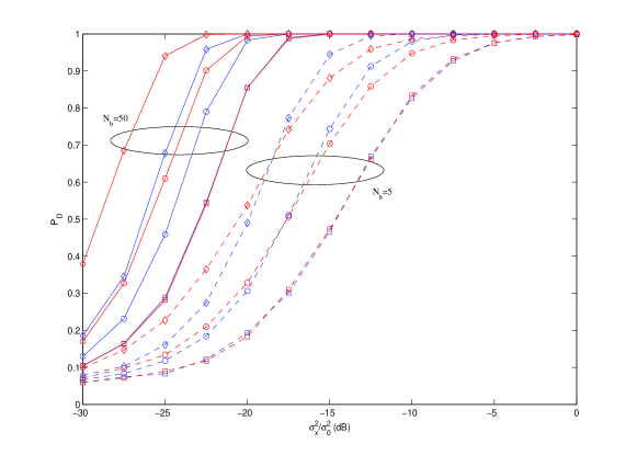
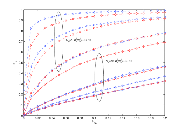
Refer to caption
Figure 4: Probability of Detection as a function of SNR for Maximally-Uncorrelated compressive detector (Blue) versus Fully-Correlated method (Red) when PFA=0.05subscript𝑃FA0.05P_{\mbox{\scriptsize FA}}=0.05. Solid curves represent the case when Nb=50subscript𝑁𝑏50N_{b}=50, and dashed curves represent the case when Nb=5subscript𝑁𝑏5N_{b}=5. The number of measurement devices is M=2𝑀2M=2 (square), M=4𝑀4M=4 (circle), and M=8𝑀8M=8 (diamond). Furthermore we choose M1=M2=M/2subscript𝑀1subscript𝑀2𝑀2M_{1}=M_{2}=M/2.
Refer to caption
Figure 5: ROC for Maximally-Uncorrelated compressive detector (Blue) versus Fully-Correlated method (Red). Solid curves represent the case when Nb=50subscript𝑁𝑏50N_{b}=50 and σx2/σ02=30superscriptsubscript𝜎𝑥2superscriptsubscript𝜎0230{\sigma_{x}^{2}}/{\sigma_{0}^{2}}=-30 dB, and dashed curves represent the case when Nb=5subscript𝑁𝑏5N_{b}=5 and σx2/σ02=15superscriptsubscript𝜎𝑥2superscriptsubscript𝜎0215{\sigma_{x}^{2}}/{\sigma_{0}^{2}}=-15 dB. The number of measurement devices is M=2𝑀2M=2 (square), M=4𝑀4M=4 (circle), and M=8𝑀8M=8 (diamond). Furthermore we choose M1=M2=M/2subscript𝑀1subscript𝑀2𝑀2M_{1}=M_{2}=M/2.

The second experiment is to study the performance loss caused by the lack of knowledge about the noise variance. Figures 6 and 7 show the performance of the proposed Maximally-Uncorrelated detection method for two cases: when the noise variance is known and when it is unknown. As we expect, the lack of knowledge of noise variance results in considerable performance degradation. However, reasonable performance is still obtained.
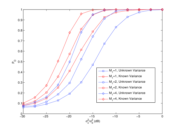
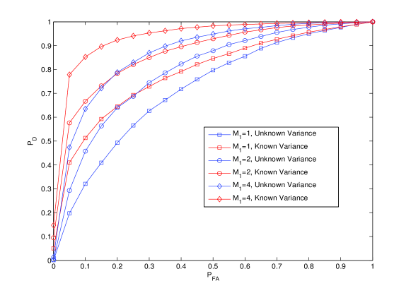
Refer to caption
Figure 6: Probability of Detection as a function of SNR for Maximally-Uncorrelated compressive detector under unknown variance (blue) versus known variance (red) when PFA=0.05subscript𝑃FA0.05P_{\mbox{\scriptsize FA}}=0.05. The number of measurements over time is Nb=5subscript𝑁𝑏5N_{b}=5. The number of rows of 𝚽ssubscript𝚽𝑠\mbox{\boldmath$\Phi$\unboldmath}_{s} is M1=1subscript𝑀11M_{1}=1 (square), M1=2subscript𝑀12M_{1}=2 (circle), and M1=4subscript𝑀14M_{1}=4 (diamond). When the variance is known we have M=M1𝑀subscript𝑀1M=M_{1} and when it is unknown we choose M2=M1subscript𝑀2subscript𝑀1M_{2}=M_{1} and therefore we have M=2M1𝑀2subscript𝑀1M=2M_{1}.
Refer to caption
Figure 7: ROC for Maximally-Uncorrelated detector for unknown variance (blue) versus known variance (red) when Nb=5subscript𝑁𝑏5N_{b}=5 and σx2/σ02=20superscriptsubscript𝜎𝑥2superscriptsubscript𝜎0220{\sigma_{x}^{2}}/{\sigma_{0}^{2}}=-20 dB. The number of rows of 𝚽ssubscript𝚽𝑠\mbox{\boldmath$\Phi$\unboldmath}_{s} is M1=1subscript𝑀11M_{1}=1 (square), M1=2subscript𝑀12M_{1}=2 (circle), and M1=4subscript𝑀14M_{1}=4 (diamond). When the variance is known we have M=M1𝑀subscript𝑀1M=M_{1} and when it is unknown we choose M2=M1subscript𝑀2subscript𝑀1M_{2}=M_{1} and therefore we have M=2M1𝑀2subscript𝑀1M=2M_{1}.

In the third experiment we study the effect of imprecise measurements and compensating it by deploying multiple measurement devices. The imprecision is modeled as described in Section IV-A. Figure 8 illustrates the ROC curves for precise (red curves) and imprecise (blue curves) measurements when σx2=1superscriptsubscript𝜎𝑥21{\sigma_{x}^{2}}=1, and σ02=100superscriptsubscript𝜎02100{\sigma_{0}^{2}}=100. The precision of all imprecise devices (blue curves) is chosen as δ1=100superscript𝛿1100\delta^{-1}=100. As expected and is clear from the comparison of the red curve with blue curve with L=1𝐿1L=1, in equivalent number of measurement devices, the imprecision in measurements results in a considerable loss in performance. However, this can be compensated by employing higher number of measurement devices. For instance, when L=3𝐿3L=3, the performance becomes equivalent to the precise case. This can be also verified by (75) in which the lower bound for performance improvement is L=3𝐿3L=3. When we go beyond this bound, e.g. L=5𝐿5L=5, the performance improves compared to the precise case.

Figure 9 shows how the probability of detection changes with the noise power for various precisions and hardware budgets of L{1,3}𝐿13L\in\{1,3\}. The black curve depicts the performance with a single precise device. Here the performance enhancement with deploying L=3𝐿3L=3 times devices has been depicted. As it can be seen for a certain δ𝛿\delta, the performance of the case of L=3𝐿3L=3 is better than a single precise device as long as σ02<ML1δ1superscriptsubscript𝜎02𝑀𝐿1superscript𝛿1\sigma_{0}^{2}<\frac{M}{L-1}\delta^{-1}. On the other hand, when the variance of noise is higher than this limit, even employing L𝐿L times devices is not enough for compensating the imprecision.
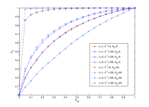
Refer to caption
Figure 8: ROC for imprecise measurements (blue curves) versus precise measurements (red curves). Solid curves represent the case when Nb=5subscript𝑁𝑏5N_{b}=5 and dashed curves represent the case when Nb=50subscript𝑁𝑏50N_{b}=50. We have chosen σx2=1superscriptsubscript𝜎𝑥21{\sigma_{x}^{2}}=1, and σ02=100superscriptsubscript𝜎02100{\sigma_{0}^{2}}=100. The number of measurement devices in precise case is M=2𝑀2M=2 with M1=M2=1subscript𝑀1subscript𝑀21M_{1}=M_{2}=1. For imprecise measurements, the device multiplicity has been chosen as L{1,3,5}𝐿135L\in\{1,3,5\}.
Refer to caption
Figure 9: Probability of detection for different precisions and device multiplicity values. The number of measurements per device is Nb=5subscript𝑁𝑏5N_{b}=5. We have chosen σx2=1superscriptsubscript𝜎𝑥21{\sigma_{x}^{2}}=1.

In the fourth experiment we study the performance of the proposed compressive detection method when the signal comes from a union of some subspaces with certain probabilities. For this experiment, the ambient dimension is N=20𝑁20N=20 and the signal dimension is K=3𝐾3K=3. In each random trial we first generate an N×N𝑁𝑁N\times N matrix with entries from a normal distribution with mean zero and variance 1/K1𝐾1/K. The elements of union set 𝒮𝒮\mathscr{S} in (83) are then Q𝑄Q different K𝐾K-size combinations of columns of the generated matrix while the signal is generated from one of them which is chosen uniformly randomly from all Q𝑄Q possible combinations. This implies that π1==πQ=1/Qsubscript𝜋1subscript𝜋𝑄1𝑄\pi_{1}=\ldots=\pi_{Q}=1/Q. The experiment is done for Q{1,10,50}𝑄11050Q\in\{1,10,50\}. We remark that the case of Q=1𝑄1Q=1 coincides with the basic case described in Section III as in this case there is no uncertainty over the subspace on which the signal lies.

Figure 10 illustrates the performance in terms of probability of detection for various values of σx2/σ02superscriptsubscript𝜎𝑥2superscriptsubscript𝜎02\sigma_{x}^{2}/\sigma_{0}^{2}. The probability of false alarm here is set to PFA=0.05subscript𝑃FA0.05P_{\mbox{\scriptsize FA}}=0.05 and the number of measurements is Nb=50subscript𝑁𝑏50N_{b}=50. The results are shown for M{2,4}𝑀24M\in\{2,4\} with M1=M2=M/2subscript𝑀1subscript𝑀2𝑀2M_{1}=M_{2}=M/2. Figure 11 also shows the ROC curves when σx2/σ02=10dBsuperscriptsubscript𝜎𝑥2superscriptsubscript𝜎0210𝑑𝐵\sigma_{x}^{2}/\sigma_{0}^{2}=-10dB. As it can be seen, as the cardinality of the subspace union set 𝒮𝒮\mathscr{S} increases, the performance of the algorithm degrades. This is in turn because as the number of possible subspaces increases, the rows of measurement matrix 𝚽𝚽\Phi are less matched to the singular vectors of the true subspace matrix.
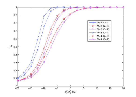
Refer to caption
Figure 10: Probability of Detection versus σx2/σ02superscriptsubscript𝜎𝑥2superscriptsubscript𝜎02\sigma_{x}^{2}/\sigma_{0}^{2} (in dB) for various numbers of measurement devices and cardinalities of the union sets. The number of measurements in time is Nb=50subscript𝑁𝑏50N_{b}=50.
Refer to caption
Figure 11: ROC curves for various numbers of measurement devices and cardinalities of the union sets. The number of measurements is Nb=50subscript𝑁𝑏50N_{b}=50 and the SNR is σx2/σ02=10superscriptsubscript𝜎𝑥2superscriptsubscript𝜎0210\sigma_{x}^{2}/\sigma_{0}^{2}=-10 dB.

VII Conclusion

The problem of random signal detection from compressive measurements when the signal is lying (or leans toward) a low dimensional subspace was studied. Having the knowledge of the subspace structure, we proposed two measurement designs and formulated the hypothesis test and its performance metrics for each of them in the case that the noise variance is unknown. We also showed how the design can be simplified in the case that the noise variance is known. We analyzed the effects of imprecise measurements and showed how it can be compensated by deploying more identical measurement devices. The problem was also generalized for the case when signal belongs to a union of finite number of subspaces with known probabilities.

Acknowledgement

This work was supported by the Finnish Funding Agency for Technology and Innovation (Tekes) under the project ”Enabling Methods for Dynamic Spectrum Access and Cognitive Radio (ENCOR)”, and the Academy of Finland under the project #251138#251138\#251138 ”Digitally-Enhanced RF for Cognitive Radio Devices (DECORA)”.

References

  • [1] D. Donoho, “Compressed sensing,” IEEE Transactions on Information Theory, vol. 52, no. 4, pp. 1289 –1306, Apr. 2006.
  • [2] E. J. Candes and T. Tao, “Near-optimal signal recovery from random projections: Universal encoding strategies?” IEEE Transactions on Information Theory, vol. 52, no. 12, pp. 5406 –5425, dec. 2006.
  • [3] E. J. Candes and M. Wakin, “An introduction to compressive sampling,” Signal Processing Magazine, IEEE, vol. 25, no. 2, pp. 21 –30, March 2008.
  • [4] M. A. Davenport, P. T. Boufounos, M. B. Wakin, and R. G. Baraniuk, “Signal processing with compressive measurements,” Selected Topics in Signal Processing, IEEE Journal of, vol. 4, no. 2, pp. 445–460, 2010.
  • [5] M. A. Davenport, M. B. Wakin, and R. G. Baraniuk, “Detection and estimation with compressive measurements,” Dept. of ECE, Rice University, Tech. Rep, 2006.
  • [6] J. Haupt and R. Nowak, “Compressive sampling for signal detection,” in Acoustics, Speech and Signal Processing, 2007. ICASSP 2007. IEEE International Conference on, vol. 3, 2007, pp. III–1509–III–1512.
  • [7] J. Paredes, Z. Wang, G. R. Arce, and B. M. Sadler, “Compressive matched subspace detection,” in Proc. 17th European Signal Processing Conference (EUSIPCO).   Citeseer, 2009, pp. 120–124.
  • [8] Z. Wang, G. R. Arce, and B. M. Sadler, “Subspace compressive detection for sparse signals,” in Acoustics, Speech and Signal Processing, 2008. ICASSP 2008. IEEE International Conference on, 2008, pp. 3873–3876.
  • [9] R. Zahedi, A. Pezeshki, and E. K. Chong, “Measurement design for detecting sparse signals,” Physical Communication, vol. 5, no. 2, pp. 64–75, 2012.
  • [10] M. Azizyan and A. Singh, “Subspace detection of high-dimensional vectors using compressive sampling,” in Statistical Signal Processing Workshop (SSP), 2012 IEEE.   IEEE, 2012, pp. 724–727.
  • [11] B. S. M. R. Rao, S. Chatterjee, and B. Ottersten, “Detection of sparse random signals using compressive measurements,” in Acoustics, Speech and Signal Processing (ICASSP), 2012 IEEE International Conference on.   IEEE, 2012, pp. 3257–3260.
  • [12] E. Arias-Castro et al., “Detecting a vector based on linear measurements,” Electronic Journal of Statistics, vol. 6, pp. 547–558, 2012.
  • [13] J. Haupt, R. Castro, R. Nowak, G. Fudge, and A. Yeh, “Compressive sampling for signal classification,” in Signals, Systems and Computers, 2006. ACSSC’06. Fortieth Asilomar Conference on.   IEEE, 2006, pp. 1430–1434.
  • [14] M. F. Duarte, M. A. Davenport, M. B. Wakin, J. N. Laska, D. Takhar, K. F. Kelly, and R. G. Baraniuk, “Multiscale random projections for compressive classification,” in Image Processing, 2007. ICIP 2007. IEEE International Conference on, vol. 6.   IEEE, 2007, pp. VI–161.
  • [15] H. Reboredo, F. Renna, R. Calderbank, and M. R. Rodrigues, “Compressive classification,” in Information Theory Proceedings (ISIT), 2013 IEEE International Symposium on.   IEEE, 2013, pp. 674–678.
  • [16] M. A. Davenport, M. F. Duarte, M. B. Wakin, J. N. Laska, D. Takhar, K. F. Kelly, and R. G. Baraniuk, “The smashed filter for compressive classification and target recognition,” in Electronic Imaging 2007.   International Society for Optics and Photonics, 2007, pp. 64 980H–64 980H.
  • [17] S. Kay, Fundamentals of statistical signal processing: detection theory.   Prentice Hall, 1998.
  • [18] H. V. Poor, An introduction to signal detection and estimation.   Springer Science & Business Media, 1994.
  • [19] L. L. Scharf, Statistical Signal Processing: Detection, Estimation, and Time Series Analysis.   Addison Wesley Publishing Company, 1991.
  • [20] S. A. Razavi, M. Valkama, and D. Cabric, “High-resolution cyclic spectrum reconstruction from sub-Nyquist samples,” in IEEE Workshop on Signal rocessing Advances in Wireless Communications (IEEE SPAWC 2013), June 16-19 2013, pp. 250–254.
  • [21] ——, “Covariance-based OFDM spectrum sensing with sub-nyquist samples,” Signal Processing, vol. 109, pp. 261 – 268, April 2015.
  • [22] E. Baransky, G. Itzhak, N. Wagner, I. Shmuel, E. Shoshan, and Y. Eldar, “Sub-Nyquist radar prototype: Hardware and algorithm,” Aerospace and Electronic Systems, IEEE Transactions on, vol. 50, no. 2, pp. 809–822, 2014.
  • [23] Y. Yu, A. P. Petropulu, and H. V. Poor, “Measurement matrix design for compressive sensing–based MIMO radar,” Signal Processing, IEEE Transactions on, vol. 59, no. 11, pp. 5338–5352, 2011.
  • [24] K. Ahmed, S. Kothuri, M. Patwary, and M. Abdel-Maguid, “Subspace compressive GLRT detector for airborne MIMO radar,” in Communications (APCC), 2010 16th Asia-Pacific Conference on.   IEEE, 2010, pp. 302–306.
  • [25] O. Bar-Ilan and Y. C. Eldar, “Sub-Nyquist radar via doppler focusing,” Signal Processing, IEEE Transactions on, vol. 62, no. 7, pp. 1796–1811, 2014.
  • [26] S. Paris, R. F. R. Suleiman, D. Mary, and A. Ferrari, “Constrained likelihood ratios for detecting sparse signals in highly noisy 3d data,” in Acoustics, Speech and Signal Processing (ICASSP), 2013 IEEE International Conference on.   IEEE, 2013, pp. 3947–3951.
  • [27] N. Wagner, Y. C. Eldar, and Z. Friedman, “Compressed beamforming in ultrasound imaging,” Signal Processing, IEEE Transactions on, vol. 60, no. 9, pp. 4643–4657, 2012.
  • [28] M. F. Duarte, M. Davenport, D. Takhar, J. N. Laska, T. Sun, K. F. Kelly, R. G. Baraniuk et al., “Single-pixel imaging via compressive sampling,” Signal Processing Magazine, IEEE, vol. 25, no. 2, pp. 83–91, 2008.
  • [29] A. M. Dixon, E. G. Allstot, D. Gangopadhyay, and D. J. Allstot, “Compressed sensing system considerations for ECG and EMG wireless biosensors,” Biomedical Circuits and Systems, IEEE Transactions on, vol. 6, no. 2, pp. 156–166, 2012.
  • [30] G. Itzhak, E. Baransky, N. Wagner, I. Shmuel, E. Shoshan, and Y. C. Eldar, “A hardware prototype for sub-Nyquist radar sensing,” in Systems, Communication and Coding (SCC), Proceedings of 2013 9th International ITG Conference on.   VDE, 2013, pp. 1–6.
  • [31] M. Mishali and Y. Eldar, “From theory to practice: Sub-Nyquist sampling of sparse wideband analog signals,” Selected Topics in Signal Processing, IEEE Journal of, vol. 4, no. 2, pp. 375 –391, April 2010.
  • [32] M. Mishali, Y. C. Eldar, and A. J. Elron, “Xampling: Signal acquisition and processing in union of subspaces,” Signal Processing, IEEE Transactions on, vol. 59, no. 10, pp. 4719–4734, 2011.
  • [33] J. A. Tropp, J. N. Laska, M. F. Duarte, J. K. Romberg, and R. G. Baraniuk, “Beyond Nyquist: Efficient sampling of sparse bandlimited signals,” Information Theory, IEEE Transactions on, vol. 56, no. 1, pp. 520–544, 2010.
  • [34] C. R. Rao and M. B. Rao, Matrix algebra and its applications to statistics and econometrics.   World Scientific, 1998.
  • [35] G. A. F. Seber, A Matrix Handbook for Statisticians.   Wiley-Interscience, 2008.
  • [36] F. Zhang, Matrix theory: basic results and techniques.   Springer Science & Business Media, 2011.
  • [37] N. L. Johnson, S. Kotz, and N. Balakrishnan, Continuous univariate distributions, vol. 2 of wiley series in probability and mathematical statistics: applied probability and statistics.   Wiley, New York,, 1995.
  • [38] M. H. DeGroot and M. J. Schervish, Probability and statistics.   Addison Wesley, 2002.
  • [39] K. Krishnamoorthy, Handbook of statistical distributions with applications.   CRC Press, 2006.
  • [40] A. W. Marshall, I. Olkin, and B. C. Arnold, Inequalities: Theory of majorization and its applications: Theory of majorization and its applications.   Springer Science & Business Media, 2010.
  • [41] L. L. Scharf and B. Friedlander, “Matched subspace detectors,” Signal Processing, IEEE Transactions on, vol. 42, no. 8, pp. 2146–2157, 1994.
  • [42] J. Haupt, R. M. Castro, and R. Nowak, “Distilled sensing: Adaptive sampling for sparse detection and estimation,” Information Theory, IEEE Transactions on, vol. 57, no. 9, pp. 6222–6235, 2011.