Gaia astrometry for stars with too few
observations – a Bayesian approach

Abstract

Context. The astrometric solution for Gaia aims to determine at least five parameters for each star, representing its position, parallax, and proper motion, together with appropriate estimates of their uncertainties and correlations. This requires at least five distinct observations per star. In the early data reductions the number of observations may be insufficient for a five-parameter solution, and even after the full mission many stars will remain under-observed, including faint stars at the detection limit and transient objects. In such cases it is reasonable to determine only the two position parameters. The formal uncertainties of such a two-parameter solution would however grossly underestimate the actual errors in position, due to the neglected parallax and proper motion.

Aims. We aim to develop a recipe to calculate sensible formal uncertainties that can be used in all cases of under-observed stars.

Methods. Prior information about the typical ranges of stellar parallaxes and proper motions is incorporated in the astrometric solution by means of Bayes’ rule. Numerical simulations based on the Gaia Universe Model Snapshot (GUMS) are used to investigate how the prior influences the actual errors and formal uncertainties when different amounts of Gaia observations are available. We develop a criterion for the optimum choice of priors, apply it to a wide range of cases, and derive a global approximation of the optimum prior as a function of magnitude and galactic coordinates.

Results. The feasibility of the Bayesian approach is demonstrated through global astrometric solutions of simulated Gaia observations. With an appropriate prior it is possible to derive sensible positions with realistic error estimates for any number of available observations. Even though this recipe works also for well-observed stars it should not be used where a good five-parameter astrometric solution can be obtained without a prior. Parallaxes and proper motions from a solution using priors are always biased and should not be used.

1 Motivation for this study

The ESA science mission Gaia, launched in December 2013, aims to determine accurate astrometry (positions, parallaxes, and proper motions) and complementary spectrophotometry for about one billion stars (Perryman et al. 2001; de Bruijne 2012). The astrometric parameters of a given star are calculated from the transits of the star’s image across the CCDs in the focal plane of Gaia. Each such field-of-view transit is essentially an instantaneous, one-dimensional measurement of the stellar position in a certain scan direction (the ‘along-scan coordinate’). The perpendicular (‘across-scan’) coordinate is also measured, but to a lower accuracy, and does not contribute significantly to the final astrometric parameters.

The path of a star on the celestial sphere, as seen from Gaia, is in the simplest case modelled by five astrometric parameters representing its position ($\alpha$, $\delta$), parallax ($\varpi$), and proper motion ($\mu_{\alpha*}$, $\mu_{\delta}$) at some chosen reference epoch. To determine all five parameters one needs at least five observations suitably distributed in time, and different scan directions are needed to derive the two-dimensional positions from the one-dimensional scans. Due to the one-year periodicity of parallax, the observations must span at least a whole year in order to reliably disentangle parallax from proper motion. The Gaia scanning law ensures that these conditions are met for stars anywhere in the sky, if the scanning lasts long enough. The nominal mission length of five years provides an ample number of observation opportunities, with an average of some 70 field-of-view transits per star. This high redundancy factor is needed to determine a large number of nuisance parameters (attitude and instrument calibration) in addition to the astrometric parameters, for judging the quality of the data, and for detecting cases (such as binaries) where the simple five-parameter model is not adequate.

However, there are inevitably many situations where a star is insufficiently observed to solve all of its five astrometric parameters. These situations include:

• Transient objects, for example extragalactic supernovae, galactic dwarf novae, and large-amplitude (Mira type) variables: these may be visible for just a few months, possibly reoccurring at a much later date.

• Faint stars near the detection limit of Gaia: nominally, all point sources brighter than 20th magnitude are detected and observed. However, since the on-board magnitude estimation has some uncertainty, stars at the detection limit may not always be observed when they transit the focal plane. Because the detection probability decreases gradually with magnitude, large numbers of faint stars will have strongly diluted observation histories.

• The first release of astrometric results, based mainly on observations collected during the first year of the mission, where most stars will be insufficiently observed.

If there are not enough observations for a given star, a simple remedy is to solve only its position ($\alpha$, $\delta$) at the mean epoch of observation. This is always possible: even in the case of a single field-of-view transit, an approximate position can be calculated by combining the along-scan and across-scan measurements.

Solving only for the two position parameters $\alpha$ and $\delta$ is equivalent to assuming that the true parallax and proper motion of the object are equal to zero. If this assumption is correct (as may effectively be the case e.g. for quasars), the resulting position estimate will be unbiased with a formal uncertainty reflecting the actual errors. However, if the true parallax and proper motion are non-zero, the estimated position will in general be biased. Its formal uncertainty (which does not depend on the parallax and proper motion value) will remain small, since the error calculus only takes into account the small observational noise of Gaia. As a result, the bias will often be many times larger than the formal uncertainty.

The solution proposed in this paper is to estimate all five parameters, while incorporating the prior information that the parallax and proper motion are typically small but non-zero quantities. Formally, this can be achieved by means of Bayes’ rule. This paper tries to answer the question how to optimally choose the prior when there are not enough Gaia observations for a regular five-parameter astrometric solution. We use numerical experiments, based on simulated observations of stars in a galactic model, to investigate the influence of the prior under different scenarios. We show that with a suitable choice of prior the solution provides sensible results in terms of both the estimated position and its calculated uncertainty.

The first release of astrometric results from the Gaia mission is expected in the summer of 2016. Due to the limited time interval covered by the early data, this release will, for the majority of stars, only contain mean positions and single-band ($G$) magnitudes. Exceptions are the Hipparcos stars, for which improved proper motions and possibly also parallaxes can be derived based on the HTPM project (Mignard 2009; Michalik et al. 2014). A similar joint reduction is possible for the Tycho-2 stars (the TGAS project; Michalik et al. 2015).

The method developed in this paper could be applied to the estimation of the positional uncertainties in the first release, but more generally to any situation where the number and distribution of observations is insufficient for a full five-parameters solution. It should be emphasised that the use of prior information in the astrometric solution always leads to biased estimates of the parameters. The proposed recipe should therefore only be used when actually needed, e.g. in the previously mentioned cases, and then only in order to obtain positions with realistic estimates of their uncertainties. These positions are valuable, e.g. for identification purposes and as a reference for ground-based observations. The resulting parallaxes and proper motions should however not be used.

2 Theory

In this section we first formulate the estimation of the astrometric parameters as a classical least-squares problem, which provides a connection to the description of the overall Gaia astrometric solution (Lindegren et al. 2012). We then show how a Gaussian prior can be introduced using Bayes’ rule. Finally we discuss the relevance and interpretation of the Gaussian prior and posterior probability densities in this context.

We use the term uncertainty for any quantitative measure of the expected degree of deviation of an estimated quantity from its true value, and reserve the term (actual) error for the signed, and in general unknown, deviation itself. In the Gaussian context the natural measure of uncertainty is the standard deviation, but as we are here dealing with strongly non-Gaussian distributions (e.g. of the true parallax values) we instead use measures based on the size of a confidence region.

2.1 Least-squares estimation of the astrometric parameters

The Gaia astrometric solution is calculated by a series of updating processes as described in Sect. 5 of Lindegren et al. (2012). In the ‘astrometric updating’ the satellite attitude and geometric calibration are assumed to be known, in which case the linearised least-squares problem for an individual star can be written in matrix form as

$$\boldsymbol{A}\boldsymbol{x}\simeq\boldsymbol{h}\,,$$ (1)

where $\boldsymbol{x}$ is a column matrix containing differential corrections to the five astrometric parameters, $\boldsymbol{h}$ is a column matrix containing the $n$ pre-adjustment observation residuals of the star, normalized by their formal uncertainties, and $\boldsymbol{A}$ is the $n\times 5$ design matrix, i.e., the partial derivative matrix row-wise normalized by the observational uncertainties. (The $\simeq$ is used in Eq. 1 because the system of equations is in general overdetermined and cannot be exactly satisfied.)

The astrometric parameters $\alpha$, $\delta$, $\varpi$, $\mu_{\alpha*}\equiv\mu_{\alpha}\cos\delta$ and $\mu_{\delta}$ refer to some chosen reference epoch $t_{\text{ep}}$, which in this paper is always taken to be the mean epoch of observation. In particular, $(\alpha,\delta)$ is the barycentric direction to the star at time $t_{\text{ep}}$. The differential corrections in $\boldsymbol{x}$ should be interpreted as $\Delta\alpha*\equiv\Delta\alpha\cos\delta$, $\Delta\delta$, $\Delta\varpi$, $\Delta\mu_{\alpha*}$, and $\Delta\mu_{\delta}$, or more rigorously using the ‘scaled modelling of kinematics’ formalism in Appendix A of Michalik et al. (2014).

The least-squares estimate of $\boldsymbol{x}$ minimizes the $\chi^{2}$ goodness-of-fit, i.e., the squared norm of the post-fit residuals $\boldsymbol{h}-\boldsymbol{A}\boldsymbol{x}$,

$$Q_{0}(\boldsymbol{x}) =\lVert\boldsymbol{h}-\boldsymbol{A}\boldsymbol{x}\rVert^{2}=(\boldsymbol{h}-\boldsymbol{A}\boldsymbol{x})^{\prime}(\boldsymbol{h}-\boldsymbol{A}\boldsymbol{x})$$

$$=\boldsymbol{h}^{\prime}\boldsymbol{h}-2\boldsymbol{x}^{\prime}\boldsymbol{b}_{0}+\boldsymbol{x}^{\prime}\boldsymbol{N}_{0}\boldsymbol{x}\,,$$ (2)

where $\boldsymbol{b}_{0}=\boldsymbol{A}^{\prime}\boldsymbol{h}$ and $\boldsymbol{N}_{0}=\boldsymbol{A}^{\prime}\boldsymbol{A}$. Putting $\partial Q_{0}/\partial\boldsymbol{x}=\boldsymbol{0}$ gives a linear system of equations,

$$\boldsymbol{N}_{0}\boldsymbol{x}_{0}=\boldsymbol{b}_{0}\,,$$ (3)

known as the normal equations, from which the least-squares estimate $\boldsymbol{x}_{0}$ can be calculated. For arbitrary $\boldsymbol{x}$ the goodness-of-fit can be written as

$$Q_{0}(\boldsymbol{x})=Q_{0}(\boldsymbol{x}_{0})+(\boldsymbol{x}-\boldsymbol{x}_{0})^{\prime}\boldsymbol{N}_{0}(\boldsymbol{x}-\boldsymbol{x}_{0})\,.$$ (4)

For badly observed stars the normal matrix $\boldsymbol{N}_{0}$ will be either ill-conditioned or singular. If it is ill-conditioned (e.g., due to a small number of nearly collinear observations), then a solution can formally be obtained. It will however have large formal uncertainties and be vulnerable to outliers, which cannot be reliably detected. The situation is different if $\boldsymbol{N}_{0}$ is strictly singular, e.g., if there are fewer observations than the number of unknowns. From a mathematical point of view, the singular problem possesses an infinite number of solutions, while algorithmically it may not be possible to determine any of them, depending on implementation choices. A remedy to both singular and ill-conditioned situations is to incorporate prior information (Sect 2.3), which always results in a unique and well-defined, albeit biased, solution.

2.2 The likelihood function

For a clean data set, with outliers filtered out or downweighted, it is reasonable to model the observational errors as independent normal random variables. For a properly calibrated instrument, the errors have mean (expected) values equal to zero and known standard deviations equal to the formal uncertainties of the observations. $\boldsymbol{h}$ is then an $n$-dimensional Gaussian, with mean value $\boldsymbol{A}\boldsymbol{x}_{\text{true}}$ and unit covariance; its probability density function (PDF) is

$$f(\boldsymbol{h}|\boldsymbol{x})=(2\pi)^{-n/2}\exp\left[-{\textstyle\frac{1}{2}}\lVert\boldsymbol{h}-\boldsymbol{A}\boldsymbol{x}\rVert^{2}\right]\propto\exp\left[-{\textstyle\frac{1}{2}}Q_{0}(\boldsymbol{x})\right]\,,$$ (5)

evaluated for $\boldsymbol{x}=\boldsymbol{x}_{\text{true}}$. Naturally, this PDF cannot be computed as $\boldsymbol{x}_{\text{true}}$ is unknown. Regarded as a function of $\boldsymbol{x}$, for the given $\boldsymbol{h}$, it is known as the likelihood of the data, designated $L(\boldsymbol{x}|\boldsymbol{h})$. Maximizing this function with respect to $\boldsymbol{x}$ is clearly equivalent to minimizing $Q_{0}(\boldsymbol{x})$, showing that $\boldsymbol{x}_{0}$ is the maximum likelihood estimate of the astrometric parameters.

2.3 Incorporating a prior

Bayes’ rule (e.g. Sivia & Skilling 2006, Sect. 3.5) expresses the posterior PDF of $\boldsymbol{x}$ as

$$f(\boldsymbol{x}|\boldsymbol{h})\propto L(\boldsymbol{x}|\boldsymbol{h})\times p(\boldsymbol{x})\,,$$ (6)

where $p(\boldsymbol{x})$ is the prior PDF and $L(\boldsymbol{x}|\boldsymbol{h})\equiv f(\boldsymbol{h}|\boldsymbol{x})$ is the likelihood of the data. The constant of proportionality is left out as it is independent of $\boldsymbol{x}$, but can be determined from the normalization constraint $\int f(\boldsymbol{x}|\boldsymbol{h})\,\text{d}\boldsymbol{x}=1$. For example, a flat (uninformative) prior $p_{0}(\boldsymbol{x})=\text{const}$ yields, by means of Eqs. (4)–(5), the posterior PDF

$$f_{0}(\boldsymbol{x}|\boldsymbol{h})=(2\pi)^{-5/2}\det(\boldsymbol{N}_{0})^{1/2}\exp\left[-{\textstyle\frac{1}{2}}Q_{0}(\boldsymbol{x})\right]\,.$$ (7)

This is a 5-dimensional Gaussian with mean value $\boldsymbol{x}_{0}$ and covariance $\boldsymbol{C}_{0}=\boldsymbol{N}_{0}^{-1}$, which reflects our knowledge of $\boldsymbol{x}$ based on the data only.

In principle, the prior PDF $p(\boldsymbol{x})$ should quantify our prior knowledge of the astrometric parameters. For example, it could be strictly zero for $\varpi<0$, while declining as a power law for large values of $\varpi$, reflecting the prior knowledge that parallaxes are generally positive, small quantities. However, in this paper we only consider Gaussian priors. This has two important advantages: (a) if both the prior PDF and the likelihood function are Gaussian, the posterior PDF is also Gaussian, which greatly simplifies its interpretation; (b) the incorporation of a Gaussian prior in the astrometric solution is straightforward, as will be shown in the following. The disadvantage is of course that a Gaussian prior is not very realistic, at least for the parallax; but with the interpretation proposed in Sect. 2.4 it is adequate for the present purpose.

Assuming a Gaussian prior with mean value $\boldsymbol{x}_{p}$ and covariance $\boldsymbol{C}_{p}$ we define

$$Q_{p}(\boldsymbol{x})=(\boldsymbol{x}-\boldsymbol{x}_{p})^{\prime}\boldsymbol{N}_{p}(\boldsymbol{x}-\boldsymbol{x}_{p})\,,$$ (8)

where $\boldsymbol{N}_{p}=\boldsymbol{C}^{-1}_{p}$. The prior probability density function is then

$$p(\boldsymbol{x})\propto\exp\left[-{\textstyle\frac{1}{2}}Q_{p}(\boldsymbol{x})\right]\,.$$ (9)

Inserting Eqs. (5) and (9) into Eq. (6) yields the posterior PDF

$$f(\boldsymbol{x}|\boldsymbol{h})\propto\exp\left[-{\textstyle\frac{1}{2}}Q_{0}(\boldsymbol{x})-{\textstyle\frac{1}{2}}Q_{p}(\boldsymbol{x})\right]\,.$$ (10)

Being the product of two Gaussian distributions, $f(\boldsymbol{x}|\boldsymbol{h})$ is clearly also Gaussian. The expected value of $\boldsymbol{x}$ can therefore be obtained by minimizing $Q(\boldsymbol{x})=Q_{0}(\boldsymbol{x})+Q_{p}(\boldsymbol{x})$, i.e., by solving

$$\partial Q(\boldsymbol{x})/\partial\boldsymbol{x} =2N_{0}(\boldsymbol{x}-\boldsymbol{x}_{0})+2N_{p}(\boldsymbol{x}-\boldsymbol{x}_{p})=0\,,$$ (11)

or

$$(\boldsymbol{N}_{0}+\boldsymbol{N}_{p})\boldsymbol{x}=\boldsymbol{b}_{0}+\boldsymbol{b}_{p}\,,$$ (12)

where

$$\boldsymbol{b}_{p}=\boldsymbol{N}_{p}\boldsymbol{x}_{p}\,.$$ (13)

It is readily shown that the covariance of the posterior estimate is given by

$$\boldsymbol{C}=(\boldsymbol{N}_{0}+\boldsymbol{N}_{p})^{-1}\,.$$ (14)

Equations (12)–(14) are the theoretical basis for the ‘joint solution’ scheme of incorporating Hipparcos and Tycho-2 priors in the Gaia data processing, developed for the HTPM and TGAS projects (Michalik et al. 2014, 2015). In the following the prior is not derived from earlier catalogues but from our expectation of the distributions of parallaxes and proper motions.

2.4 Interpretation of the Gaussian probability densities

In the following it is assumed that the prior distribution of parallaxes is Gaussian with mean value $\varpi_{p}=0$ and standard deviation $\sigma_{\varpi,p}$ equal to the square root of the corresponding (third) diagonal element of $\boldsymbol{C}_{p}$. (Similar assumptions are made concerning the prior distributions of the proper motion components.) Clearly this is not very realistic, as it implies that, a priori, there is a 50% probability that the parallax is negative. However, the same Gaussian prior also means that there is a 90% probability that the true parallax is less than $1.28\sigma_{\varpi,p}$, and a 99% probability that it is less than $2.33\sigma_{\varpi,p}$. These latter statements are obviously meaningful, and provide a useful quantification of the expected smallness of the parallax, even though the distribution of true parallaxes is far from Gaussian.

A similar interpretation can be made of the Gaussian posterior PDF in Eq. (10). Although the actual error distribution of the Bayesian solution may be strongly non-Gaussian, this PDF can still be used to construct sensible confidence regions. In this work we are primarily interested in the positions and ignore the estimated parallaxes and proper motions. As the position uncertainty may be quite anisotropic, it should not be given as a single value but as a confidence region, for example a confidence ellipse, such that the true value is contained within that region with a certain degree of confidence $P$.

In this work we choose to work with a confidence level of 90% ($P=0.9$). This means that the (Gaussian) posterior covariance should be such that a 90% confidence ellipse constructed from it will, in 90% of the cases, contain the true position. The choice of $P=0.9$ is arbitrary, and a different value (e.g., 0.8, 0.95, or 0.99) would in general require a different covariance matrix in order to correctly characterise the errors at that $P$-value. Only in the case of Gaussian posterior errors would a single covariance matrix correctly describe the error distribution for different values of $P$.

The confidence ellipse can be constructed from the positional covariance (the $2\times 2$ submatrix of $\boldsymbol{C}$) as described in Press et al. (2007). In particular, for $P=0.9$ the semi-axes of the ellipse are $\sqrt{-2\ln(1-P)}\simeq 2.146$ times the square roots of the singular values of the positional covariance matrix. Inside the ellipse we have $Q(\boldsymbol{x})-Q_{\text{min}}<-2\ln(1-P)\simeq 4.605$.

A good astrometric solution should not only be as accurate as possible but also have formal uncertainties that characterize the actual errors correctly. Thus our general approach is to optimise the prior PDF for both goals. The formal uncertainties (positional covariance matrix) of the resulting posterior estimate should be such that the 90% confidence ellipse, computed as described above, contains the true position with 90% probability.

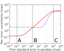
Figure 1: Behaviour of the Bayesian position estimate as a function of the parallax prior uncertainty $\sigma_{\varpi,p}$, for stars within one direction and magnitude bin (Table 1). Blue dashed curve: 90th percentile of the actual position errors. Red solid curve: semi-major axis of the 90% confidence ellipse. The priors labeled A, B, and C refer to the panels in Fig. 2.

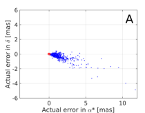
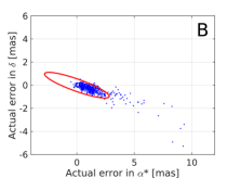
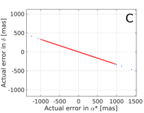
Figure 2: Distribution of position errors for the three cases A, B, and C in Fig. 1. Blue dots: individual astrometric errors. Red curve: 90% confidence ellipse. Prior A is too tight and essentially gives a two-parameter solution. Prior B at the intersection of the curves in Fig. 1 (semi-major axis of the 90% confidence ellipse equals the 90th percentile of the actual errors) produces sensible error estimates. Prior C is too loose and yields a degenerate solution – although not visible in the diagram, 90% of the points are contained in the extremely elongated ellipse.

Table 1: Parameters of the single direction experiments reported in Figs. 1, 2, and 3.

Celestial coordinates
Equatorial:	$\alpha=157.5\degr$	$\delta=0.0\degr$
Ecliptic:	$\lambda=159.2\degr$	$\beta=-8.8\degr$
Galactic:	$l=245.7\degr$	$b=+46.5\degr$
Pencil beam parameters
Radius of beam:		1°
Magnitude range:		$G=15\pm 0.5$ mag
Number of stars in GUMS:		458
Observations according to Gaia’s Nominal Scanning Law
Date and time (UTC)	FOV	pos. angle	#
2014-Oct-30 17.0h	P	230°	1
2014-Oct-30 18.8h	F	230°	1
2014-Nov-20 17.0h	P	156°	2
2014-Nov-20 18.8h	F	156°	2
2014-Dec-19 16.6h	P	247°	3
2014-Dec-19 18.4h	F	247°	3
2015-Apr-29 05.2h	P	341°	4
2015-Apr-29 07.0h	F	342°	4
2015-May-23 18.9h	F	065°	5
2015-Jun-21 04.9h	P	344°	6
2015-Jun-21 06.7h	F	344°	6
2015-Nov-09 06.1h	P	238°	7
2015-Nov-09 07.9h	F	238°	7
2015-Dec-29 11.8h	P	243°	8
2015-Dec-29 13.6h	F	244°	8

3 Prior in an astrometric solution

3.1 Framework and basic assumptions

In order to systematically evaluate the effect of the prior on the astrometric performance we have developed Matlab scripts which compute the Bayesian position estimates for a set of simulated stars. The true stellar parameters are taken from the Gaia Universe Model Snapshot (GUMS; Robin et al. 2012). Gaia observations are simulated using the Gaia Nominal Scanning Law (de Bruijne et al. 2010) with initial precession and scan phase conditions consistent with the real mission from October 2014 until the end of 2015. The astrometric parameters are estimated as described in Sect. 2. For the initial analysis it is assumed that the spacecraft attitude and instrument calibration are known, so that the solution only involves the five astrometric parameters of each star. The posterior covariance and astrometric parameters are computed and compared for different combinations of magnitude range, position on the sky, as well as number of observations and their temporal distribution.

We then experiment with varying priors for parallax and proper motion in the different scenarios. Applying such prior knowledge aids the astrometric solution by constraining parallax and proper motion to small values, without forcing them to be strictly zero. In the present experiments the prior parallax and proper motion are centred on zero with Gaussian uncertainties $\sigma_{\varpi,p}$ and $\sigma_{\mu,p}$, respectively. The largest known stellar parallax is 768 mas but typical parallaxes are much smaller than that. $\sigma_{\varpi,p}$ is therefore in the few mas regime. The proper motion depends on the parallax through the expression for the transverse space velocity $v_{T}=A\mu/\varpi$, where $A\simeq 4.74$ km s^-1 yr. Linear velocities in the Galaxy are of the order of 30–300 km s^-1 and we therefore typically expect $\mu/\varpi\simeq 6$–$60$ yr^-1. At magnitude 15 the median ratio in GUMS is 10 yr^-1. For the ratio $\mathcal{R}=\sigma_{\mu,p}/\sigma_{\varpi,p}$ we have experimented with values in the range 1–60 yr^-1 and found the results to be relatively insensitive to this choice. Using a value of $\mathcal{R}=10$ yr^-1 provides reasonable results in all cases, and we adopt this value in the rest of this paper.

3.2 Behaviour of the solution as a function of the prior

For an initial understanding of how the astrometric results depend on the choice of prior we show a representative example from our experiments. For one particular position on the sky we took stars from GUMS of a certain apparent $G$ magnitude in a one degree pencil beam (Table 1). The framework described in Sect. 3.1 was used to simulate shorter or longer observation intervals of Gaia. Using one to eight distinct transits (Table 1, bottom section), we obtain the actual errors and formal uncertainties of the resulting position parameters for each observation interval as a function of prior size $\sigma_{\varpi,p}$.

Figures 1 and 2 give the detailed results for an observation interval containing two transits that are distinct in time and angle (#1 and #2 in Table 1). Figure 1 summarizes how the actual errors and formal uncertainties vary as functions of $\sigma_{\varpi,p}$. The sigmoid shape of the red curve describing the formal uncertainties is analytically explained in Appendix A.

Let us first look at the behaviour of the solution when a very tight prior is applied, e.g. $\sigma_{\varpi,p}=0.01$ mas as indicated by the vertical line at A in Fig. 1. The resulting solution (both with regard to the actual position errors and their formal uncertainties) is practically equivalent to solving only for the two position parameters, where the parallax and proper motion are implicitly assumed to be zero. In this regime the actual errors (dashed curve) are much larger than the formal position uncertainties (solid curve) due to the neglected parallax and proper motion. This is further illustrated by the top panel (prior A) in Fig. 2, where the 90% confidence ellipse (red) only contains a small fraction of the actual errors (blue dots).

Moving from tight to looser priors (increasing $x$-axis values in Fig. 1), the solution becomes less constrained and the formal uncertainties necessarily increase. For $\sigma_{\varpi,p}\geq 30$ mas the size of the actual errors increases, since with two distinct transits the Gaia data alone are insufficient to determine all five parameters in the solution. Using a very loose prior, for example prior C illustrated in the bottom panel of Fig. 2, the astrometric solution becomes almost degenerate, though the formal uncertainties still correctly describe the actual errors. The intersection point marked with letter B in Fig. 1 would be a reasonable compromise, where the solution is as precise as permitted by the available data, while the formal uncertainties correctly characterize the actual position errors. This is illustrated in the middle panel (prior B) of Fig. 2, where most of the actual error points lie within the confidence ellipse.

The actual position errors in panels A and B in Fig. 2 are skewed in a direction depending on the position of the satellite in its orbit around the Sun. The offset of the error cloud from the origin depends on the sizes of the parallaxes and proper motions.

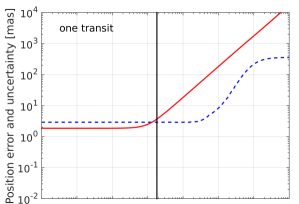
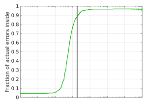
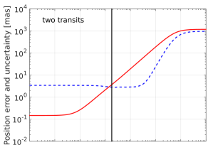
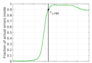
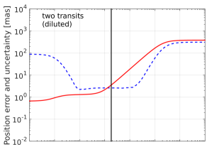
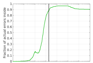
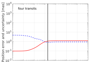
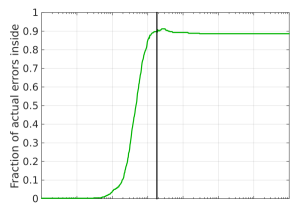
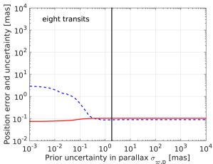
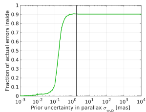
Figure 3: Behaviour of the position error and uncertainty with varying priors, for stars in the direction and magnitude bin specified in Table 1. The rows display the behaviour for different numbers of distinct transits: one, two, two (diluted), four, and eight distinct transits. The diluted case uses the first and last transit from Table 1 instead of the first two transits. Left column: size of actual position errors (blue dashed) and their formal uncertainties (red solid), for stars in the same direction and magnitude bin, as a function of the prior uncertainty. Right column: fraction of actual errors contained by the formal error ellipse. The optimum prior $\sigma_{\varpi,F90}$ is chosen based on the observation interval containing two distinct consecutive transits (second row). This prior is replicated in all other panels.

3.3 Criterion for the optimum prior uncertainties

The two quantities represented by the dashed and solid curves in Fig. 1 are not exactly comparable: one is the radius of the circle, centred on zero, that contains 90% of the actual errors; the other is the semi-major axis of the confidence ellipse. Using their point of intersection to optimise the prior, as suggested in the previous section, is therefore slightly illogical. We have instead adopted a different and much simpler criterion based on the confidence ellipse: the optimum prior should be such that 90% of the actual position errors are contained by the 90% confidence ellipse as calculated from the covariance matrix. The smallest $\sigma_{\varpi,p}$ fulfilling this condition is in the following called $\sigma_{\varpi,F90}$ and is illustrated in the second row of Fig. 3. The left diagram replicates the curves for two distinct transits previously shown in Fig. 1. The right diagram shows the corresponding fraction of actual errors contained in the 90% confidence ellipse. The prior choice $\sigma_{\varpi,F90}$, marked by the solid vertical line and replicated in all panels of the figure, is in fact quite close to the intersection of the two curves in the left diagram.

So far we have limited our discussion to a scenario with two distinct transits. This is the case where the prior information is expected to be most critical: two distinct along-scan observations may suffice to determine a sensible position, but are always insufficient for a full five-parameter solution; on the other hand, three distinct transits in principle already allow a five parameter solution if both along- and across-scan information is used. We adopt $\sigma_{\varpi,F90}$ based on the two-transit case and use it also in other scenarios with more or less observations. That the same prior works in these cases has been verified through simulations. Examples are given in Fig. 3, where the different rows show the behaviour of the astrometric solution for observation intervals containing one, two, four, and eight distinct transits, including one diluted case of two transits separated by 14 months. The prior $\sigma_{\varpi,F90}$ determined from the two-transit scenario, and indicated by the solid vertical line in all panels, yields in all cases a solution where the size of the actual position errors (as measured by the 90th percentile) is close to its minimum, together with a realistic 90% confidence ellipse.

It is also evident that $\sigma_{\varpi,F90}$ is a lower limit for a suitable prior. Increasing $\sigma_{\varpi,p}$ by up to a factor $\sim$10 keeps the actual position errors at the same level while providing the same or a more conservative formal uncertainty estimate, whereas using a smaller prior would underestimate the errors. In Appendix A we briefly address the effect of the prior uncertainty on the posterior error estimate from an analytical point of view.

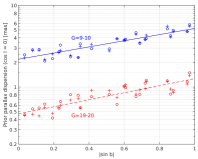
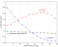
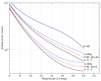
Figure 4: Illustrations of the all-sky approximation to the parallax prior $\sigma_{\varpi,F90}$. Left: Representative example of the linear fit in Eq. (15) of the logarithm of the parallax prior $\sigma_{\varpi,F90}$ as a function of galactic latitude $b$, for two magnitude ranges $G=9$–$10$ (blue), and $G=19$–$20$ (red). The small dependence on galactic longitude (the third term in Eq. 15) has been subtracted leaving no systematic dependence on galactic longitude $l$, as shown by the different symbols ($\circ$ for $\cos l>0$, + for $\cos l<0$). Middle: Variations of the coefficients $s_{0}$, $s_{1}$, and $s_{2}$ with $G$ magnitude, and polynomial fits according to Eqs. (16)–(18). Right: The prior $\sigma_{\varpi,F90}$ in Eq. (15) as a function of magnitude, for different latitudes (lowest to highest group: $b=0\degr$, 30°, and 90°) and different longitudes (black solid $l=0\degr$, red dashed 90°, blue dotted-dashed 180°).

3.4 Prior uncertainty as function of magnitude and direction

In Sect. 3.3 we described the determination of an optimum value of $\sigma_{\varpi,p}$, called $\sigma_{\varpi,F90}$, for one particular direction and magnitude interval. We repeated this experiment for different directions and magnitude bins ($G=6$–20, in steps of 1 mag). We find that 48 directions uniformly distributed on the sky are sufficient to sample the large-scale structures of the underlying Galaxy model. As expected, $\sigma_{\varpi,F90}$ is a strong function of magnitude (fainter stars being on average more distant), and to a lesser extent dependent on direction (because of extinction and the spatial distribution of stars in our Galaxy). For a given magnitude bin we find that a reasonable fit to the individual data points is provided by

$$\log_{10}\sigma_{\varpi,F90}=s_{0}+s_{1}|\sin b|+s_{2}\cos b\cos l\,$$ (15)

(see the left panel of Fig. 4). The variations of the coefficients $s_{0}$, $s_{1}$, and $s_{2}$ with $G$ magnitude bins are shown in the middle panel of Fig. 4. They are well approximated by simple polynomials in $G$:

$$s_{0}(G) =2.187-0.2547G+0.006382G^{2}$$ (16)

$$s_{1}(G) =0.114-0.0579G+0.01369G^{2}-0.000506G^{3}$$ (17)

$$s_{2}(G) =0.031-0.0062G$$ (18)

The size of the fitted $\sigma_{\varpi,F90}$ prior is illustrated in the right panel of Fig. 4. For the astrometric solution of an arbitrary star of magnitude $G$ at galactic coordinates $(l,b)$ the prior normal matrix to be used in Eqs. (12)–(13) is then

$$\boldsymbol{N}_{p}=\textrm{diag}(0,\ 0,\ \sigma_{\varpi,F90}^{-2},\ \sigma_{\mu,F90}^{-2},\ \sigma_{\mu,F90}^{-2})\,,$$ (19)

where $\sigma_{\varpi,F90}(l,b,G)$ is given by Eqs. (15)–(18), and $\sigma_{\mu,F90}=\mathcal{R}\sigma_{\varpi,F90}$, where $\mathcal{R}=10$ yr^-1.

An extension of $\sigma_{\varpi,F90}(l,b,G)$ to fainter stars is non-trivial, since GUMS is only complete to $G=20$. For fainter stars the value at $G=20$ should be used since it provides a conservative (over)estimate. For stars brighter than $G=6$ it might be preferable to make solutions directly using priors from the Hipparcos and Tycho-2 catalogues.

In principle more sophisticated priors could be considered, which take into account photometric, spectroscopic, or other auxiliary information. For example, blue stars have on average smaller parallaxes than red stars, and for identified extra-galactic objects the prior uncertainty could be much smaller. However, such information may be unavailable precisely in the cases where a prior is needed. On the other hand, a direction and an approximate magnitude are always available, and allow us to define a general prior.

Table 2: Simulation results for stars with 95% diluted five year observation histories. The spacecraft attitude was determined by a separate solution from well-observed stars. A prior uncertainty $\geq\sigma_{\varpi,F90}$ provides a sensible solution for all stars.

Prior $\sigma_{\varpi,p}$	Fraction in 90% conf. ellipse			Actual position errors [mas]
	$G\simeq 11$	$G\simeq 15$	$G\simeq 19$	$G\simeq 11$	$G\simeq 15$	$G\simeq 19$
Subset of stars with $\leq$4 field-of-view transits
none (2 parameters)	0.5%	1.8%	13.5%	33.0	16.3	15.2
$0.01$ mas	1.5%	3.5%	14.3%	21.8	12.1	14.8
$\sigma_{\varpi,F90}$	90.1%	91.4%	91.2%	7.6	4.3	7.6
$10\sigma_{\varpi,F90}$	92.7%	93.3%	94.4%	8.4	5.2	10.5
$1000$ mas	92.5%	93.0%	93.3%	8.6	7.4	15.5
Subset of stars with ¿4 field-of-view transits
none (2 parameters)	0.3%	0.8%	8.6%	21.0	11.3	9.7
$0.01$ mas	3.1%	5.4%	10.4%	6.7	5.0	8.9
$\sigma_{\varpi,F90}$	89.4%	89.9%	90.3%	0.2	0.3	1.6
$10\sigma_{\varpi,F90}$	89.5%	89.8%	90.5%	0.2	0.3	2.0
$1000$ mas	89.5%	89.8%	90.0%	0.2	0.3	2.2

Table 3: Global astrometric solutions using 12 months of simulated Gaia data. The attitude is determined as part of the solution. Here the prior uncertainty needs to be relaxed to $10\sigma_{\varpi,F90}$ to obtain a sensible solution. Columns as in Table 2.

Prior $\sigma_{\varpi,p}$	Fraction in 90% conf. ellipse			Actual position errors [mas]
	$G\simeq 11$	$G\simeq 15$	$G\simeq 19$	$G\simeq 11$	$G\simeq 15$	$G\simeq 19$
Subset of stars with $\leq$4 field-of-view transits
$\sigma_{\varpi,F90}$	76.5%	86.8%	92.4%	1.2	0.7	2.0
$10\sigma_{\varpi,F90}$	89.1%	90.4%	94.3%	1.4	1.1	4.2
$1000$ mas	89.7%	89.8%	90.6%	3.8	3.4	17.7
Subset of stars with ¿4 field-of-view transits
$\sigma_{\varpi,F90}$	32.3%	53.3%	88.0%	0.2	0.2	0.8
$10\sigma_{\varpi,F90}$	88.6%	89.3%	90.4%	0.1	0.2	1.0
$1000$ mas	88.7%	89.4%	90.0%	0.1	0.2	1.1

4 Simulation of potential application scenarios

In this section we demonstrate the feasibility of the proposed method based on simulations of potential applications. We used GUMS to provide simulated ‘true’ parameters for a large catalogue of stars of different magnitude classes, where we include the $5\times 10^{5}$ brightest stars fainter than each of the magnitudes $G=11$, 15, and 19, respectively. The software package AGISLab (Holl et al. 2012; Bombrun et al. 2012) was used to simulate Gaia observations and to perform a global astrometric solution.

In Sect. 1 we described three situations where the Bayesian approach might be useful: transient objects, faints stars at the detection limit, and the processing of short stretches of Gaia data. The first two situations are similar to the diluted case presented in Sect. 3.3. When solving the astrometric parameters we can assume that an accurate satellite attitude is known from a previous solution of well-observed stars. The third situation applies to the first release of Gaia data, where the spacecraft attitude must be obtained together with the astrometric parameters from the same (insufficient) data, and therefore is much less accurate than in the previous scenario. We therefore performed two distinct sets of simulations described hereafter.

4.1 Stars with very diluted observation histories

Here we use an attitude determined by a five year solution of simulated Gaia data without prior. We then compute the astrometric parameters without changes to the attitude (a so-called secondary solution) for stars with a highly diluted observation history. The dilution is simulated by assigning each field of view transit a 95% probability of being removed from the solution. The average number of retained transits per star is $\simeq 4.4$.

We made a solution using the optimum prior according to Sect. 3.4. Additionally we experimented with a very tight prior ($\sigma_{\varpi,p}=0.01$ mas, analogous to case A in Fig. 2) and a very loose prior ($\sigma_{\varpi,p}=1000$ mas, analogous to case C in Fig. 2) to check the behaviour of the solution in these extreme cases. For comparison we also made two runs without any prior, one in which only the two position parameters were determined, and one with all five astrometric parameters. In the latter case it was not possible to determine a unique astrometric solution for all stars, as explained at the end of Sect. 2.1.

Table 2 summarizes our results. Only the results for the position estimates are shown. When using a very tight prior the results are very similar to a two parameter solution. The formal uncertainties computed in this solution grossly underestimate the actual errors. Using the optimum prior $\sigma_{\varpi,F90}$ (or ten times its value) instead yields sensible estimates of the uncertainties. The use of this prior not only provides improved uncertainties, but also reduces the actual errors compared with a two-parameter solution (or a very tight prior). This somewhat surprising behaviour can be understood from the three bottom left panels in Fig. 3: using a non-zero prior uncertainty provides the necessary freedom for the solution to accommodate non-zero parallaxes and proper motions and hence to reduce the actual position errors.

With a very loose prior of one arc-second the Bayesian approach still results in a numerically stable astrometric solution (which is not true for solutions without any prior), including realistic estimates of the positional uncertainties. However the actual errors are up to a factor two larger than when using a well-chosen prior.

4.2 The first data release

Another possible application of the proposed method is for the planned first release of intermediate Gaia data. As this may be based on too short a stretch of data for a reliable five-parameter solution, the release is targeted to give only positions and mean $G$. We propose the use of a prior to ensure that the one year global solution provides a sensible formal position uncertainty for all stars. This scenario is different compared to Sect. 4.1, since the attitude must now be determined from the same observations as the astrometric parameters, a so-called primary solution. We simulate this through a global solution assuming one year of Gaia observations with 20% of dead time, and using priors of varying size.

Table 3 summarizes our results. Contrary to Sect. 4.1 and Table 2 we now find that the prior $\sigma_{\varpi,F90}$ constrains the solution too much. It appears that the prior uncertainty needs to be increased to account for the larger attitude errors caused by the unknown parallax and proper motion contributions. Empirically we find that a ten fold increase of the prior uncertainty provides the necessary relaxation of the constraint and allows the solution to fulfill the criteria for a sensible astrometric result.

5 Conclusions

In this paper we discuss the astrometric solutions for stars with an insufficient number of Gaia observations. This will be the case for the majority of stars in the first data release of Gaia data, but is also an important issue during later stages of the mission, e.g. for transient objects that are only observed in their bright phases, and stars close to the detection limit. In all these cases one can still obtain very valuable position estimates, either by solving only for the position parameters or through the use of priors for the remaining parameters. In fact, solving only for the position parameters is equivalent to assuming that the parallax and proper motion are exactly zero, in other words to the use of prior values equal to zero with infinite weights. Using a more carefully selected prior improves the quality of the astrometric solution for these stars. Very specifically, it provides an elegant way to ensure that the position estimates obtain formal uncertainties that correctly characterize the actual errors.

Prior information is incorporated in the astrometric solution using Bayes’ rule. For practical reasons the prior probability distributions are taken to be Gaussian. Moreover, they are always centred on zero, since any other choice would necessarily involve additional assumptions and thus be even more arbitrary. For objects with negligible parallax, such as quasars, it is a conservative choice.

We analyse the influence of different priors on the astrometric solutions, based on numerical experiments with realistic distributions of stellar parameters from the Gaia Universe Model Snapshot (GUMS). To optimize the prior we require that 90% of the actual position errors are included in the 90% confidence region calculated from the (Gaussian) posterior probability density, i.e. from the formal covariance matrix. Using the resulting prior ($\varpi_{p}=0\pm\sigma_{\varpi,F90}$) we find that non-singular five-parameter astrometric solutions can be obtained, with reasonable estimates of the position uncertainties, for any star that is observed in at least one field-of-view transit. Using this prior slightly reduces the actual position errors, compared with a two-parameter solution. The solution is robust to using a larger prior uncertainty than $\sigma_{\varpi,F90}$, and in some cases (depending on the attitude estimation) a ten fold increase is motivated (Sect. 4.2).

The choice of a 90% confidence level for the position errors is arbitrary and it would be possible to optimize the prior for any other desired percentage. The 10% stars falling outside the confidence ellipse cannot easily be identified from the data and could be considered outliers. In statistical uses of the data, 90% provides a good compromise between keeping a reasonably small fraction of outliers and maintaining a good characterization of the positional uncertainties for most stars. A higher confidence level would decrease the fraction of outliers, but at the expense of a rapidly growing confidence region due to the non-Gaussian nature of the actual position errors.

Like any solution using a prior, the resulting astrometric parameters are in general biased. Using a reference epoch centred on the observations, the position bias is of the order of the neglected parallax, or at most a few mas in typical cases. As discussed below this is acceptable. In order to obtain realistic uncertainties of the positions, it is necessary to introduce the parallax and proper motion as formal parameters in the solution. This means that posterior estimates are also provided for these. However, the resulting parallaxes and proper motions are in general so strongly biased by the prior that they become physically meaningless, and they should therefore not be used.

For the first release of Gaia data, consisting mainly of position information and $G$ magnitudes, small biases in the resulting position estimates are fully acceptable and unavoidable. For future releases however, where a full solution can be determined for most of the stars, it is important to determine attitude and geometric calibration parameters as part of the primary solution, by using only the stars with a sufficient amount of observations. For all of these it is mandatory that no prior is used. Any star with insufficient observations, which requires the use of a prior for the solution, must be part of a separate (secondary) update, in which the attitude and calibration are not modified. For the secondary stars with insufficient data, the $\varpi_{p}=0\pm\sigma_{\varpi,F90}$ prior will however allow us to obtain sensible position estimates with well-characterized formal uncertainties.

Appendix A Analytical illustration

To analytically study how the prior affects the posterior position uncertainty, we consider a simplified case where the solution includes only two astrometric parameters: one component of position (e.g. $\delta$) and the parallax ($\varpi$). The normal matrix incorporating the prior $\boldsymbol{N}_{p}=\textrm{diag}(0,\sigma_{\varpi,p}^{-2})$, similar to Eq. (19), then takes the form

$$\boldsymbol{N}_{0}+\boldsymbol{N}_{p}=\frac{1}{1-\rho^{2}}\left(\begin{array}[]{cc}\sigma_{\delta}^{-2}&\dfrac{-\rho}{\sigma_{\delta}\sigma_{\varpi}}\\[12.0pt] \dfrac{-\rho}{\sigma_{\delta}\sigma_{\varpi}}&\sigma_{\varpi}^{-2}+\left(1-\rho^{2}\right)\sigma_{\varpi,p}^{-2}\end{array}\right)\,,$$ (20)

where $\sigma_{\delta}$ and $\sigma_{\varpi}$ are the standard errors of the position and parallax, respectively, and $\rho$ is the correlation coefficient; all these quantities are based on the data only. Calculating the posterior covariance matrix using Eq. (14) we find the position uncertainty

$$\sigma_{\delta,\,\textrm{posterior}}=\sigma_{\delta}\sqrt{1-\frac{\rho^{2}}{1+\left(\sigma_{\varpi,p}/\sigma_{\varpi}\right)^{2}}}\,.$$ (21)

This formula agrees with our numerical experiments. In particular it reproduces the behaviour of the position uncertainty shown in Figs. 1 and 3, featuring a monotonically increasing $\sigma_{\delta,\,\textrm{posterior}}$ between two asymptotic values, $\sigma_{\delta}\sqrt{1-\rho^{2}}$ and $\sigma_{\delta}$, as the prior goes from very tight to very loose. Equation (21) implies that the improvement in the positional uncertainty gained by using the parallax prior depends only on the correlation coefficient $\rho$ and the ratio of the parallax prior to the formal uncertainty without prior, $\sigma_{\varpi,p}/\sigma_{\varpi}$. For uncorrelated data, no improvement is possible, as $\sigma_{\delta,\,\textrm{posterior}}=\sigma_{\delta}$ for $\rho=0$.

Similar arguments hold for the general five-parameter solution, except that they cannot be demonstrated so easily.