LPNHE/2015–01
HU-EP–15/32
DESY 15–116

Muon $g-2$ Estimates :
Can One Trust Effective Lagrangians and Global Fits?

M. Benayoun^a, P. David^a,b, L. DelBuono^a, F. Jegerlehner^c,d
a LPNHE des Universités Paris VI et Paris VII, IN2P3/CNRS, F–75252 Paris, France
^b LIED, Université Paris-Diderot/CNRS UMR 8236, F–75013 PARIS, France
^c Humboldt–Universität zu Berlin, Institut für Physik, Newtonstrasse 15, D–12489 Berlin, Germany
^d Deutsches Elektronen–Synchrotron (DESY), Platanenallee 6, D–15738 Zeuthen, Germany

Previous studies have shown that the Hidden Local Symmetry (HLS) Model, supplied with appropriate symmetry breaking mechanisms, provides an Effective Lagrangian (BHLS) which encompasses a large number of processes within a unified framework. Based on it, a global fit procedure allows for a simultaneous description of the $e^{+}e^{-}$ annihilation into 6 final states – $\pi^{+}\pi^{-}$, $\pi^{0}\gamma$, $\eta\gamma$, $\pi^{+}\pi^{-}\pi^{0}$, $K^{+}K^{-}$, $K_{L}K_{S}$ – and includes the dipion spectrum in the $\tau$ decay and some more light meson decay partial widths. The contribution to the muon anomalous magnetic moment $a_{\mu}^{\rm th}$ of these annihilation channels over the range of validity of the HLS model (up to 1.05 GeV) is found much improved in comparison to the standard approach of integrating the measured spectra directly. However, because most spectra for the annihilation process $e^{+}e^{-}\to\pi^{+}\pi^{-}$ undergo overall scale uncertainties which dominate the other sources, one may suspect some bias in the dipion contribution to $a_{\mu}^{\rm th}$, which could question the reliability of the global fit method. However, an iterated global fit algorithm, shown to lead to unbiased results by a Monte Carlo study, is defined and applied succesfully to the $e^{+}e^{-}\to\pi^{+}\pi^{-}$ data samples from CMD2, SND, KLOE, BaBar and BESSIII. The iterated fit solution is shown to further improve the prediction for $a_{\mu}$, which we find to deviate from its experimental value above the $4\sigma$ level. The contribution to $a_{\mu}$ of the $\pi^{+}\pi^{-}$ intermediate state up to 1.05 GeV has an uncertainty about 3 times smaller than the corresponding usual estimate. Therefore, global fit techniques are shown to work and lead to improved unbiased results.

1 Introduction

As is well known, the Standard Model is the gauge theory which covers the realm of weak, electromagnetic and strong interactions among quarks, leptons and the various gauge bosons (gluons, photons, $W^{\pm}$, $Z^{0}$). In energy regions where perturbative methods apply, the Standard Model (SM) allows to yield precise estimates for several physical effects, sometimes with accuracies of the order of a few 10^-12. In contrast, in energy regions where the non–perturbative regime of QCD is involved, getting similar precision may become challenging. This is the case for the low energy part of the photon hadronic vacuum polarization (HVP); this HVP plays a crucial role in determining the theoretical value for the muon anomalous moment $a_{\mu}$, one of the best measured particle properties.

Fortunately, getting precise estimates in the low energy hadron SM sector is not completely out of reach as exemplified by the Chiral Perturbation Theory (ChPT)[1, 2] which is rigorously the low energy limit of QCD, valid up to 400 $\div$ 500 MeV but lets the resonance region outside its scope. Lattice QCD (LQCD) is also a promising method under rapid development which already allows to perform precise computations at low (and very low) energies [3]. Interesting LQCD estimates for the HVP’s of the three leptons have already been produced [4, 5] which clearly show that LQCD reaches results in accord with expectations; this is especially striking for $a_{\mu}$ with, however, still unsatisfactory uncertainties [4].

So, much progress remains to be done before LQCD evaluations can compete with the accuracy of the experimental measurements already available [6, 7] or, a fortiori, with those expected in a near future at Fermilab [8, 9] or, slightly later, at J–PARC [10]. Since lattice QCD is intrinsically an Euclidean approach, it is intrinsically unable to account for the existing rich amount of low energy hadronic data in the non-perturbative time-like region, i.e. from thresholds to 2 $\div$ 3 GeV. Therefore, other methods, able to encompass large fractions of the physics from this important energy region, are valuable.

A natural approach to this issue is provided by Effective Lagrangians which cover the resonance region. Such Effective Lagrangians should be constructed so as to preserve the symmetry properties of QCD as already done by standard ChPT, however only valid up to the $\eta$ mass region. As it includes meson resonances, the Resonance Chiral Perturbation Theory (R$\chi$PT) [11] is an appropriate framework to study $e^{+}e^{-}$ annihilations from their respective thresholds up to the intermediate energy region.

It has been proven [12] that the coupling constants occuring at order $p^{4}$ in ChPT are saturated by low lying meson resonances of various kinds as soon as they can contribute. This emphasizes the role of the fundamental vector meson nonet (V) and confirms the relevance of the Vector Meson Dominance (VMD) concept in low energy physics.

On the other hand, it has been proven [11] that the Hidden Local Symmetry (HLS) Model [13] and R$\chi$PT are equivalent provided consistency with the QCD asymptotic behavior is incorporated. It thus follows that the HLS model is also a motivated and constraining QCD rooted framework. As the original HLS Model only deals with the lowest mass resonances, it provides a framework for the $e^{+}e^{-}$ annihilations naturally bounded by the $\phi$ mass region – i.e. up to $\simeq 1.05$ GeV.

The non–anomalous [14] and anomalous [15] sectors of the HLS Model open a wide scope and can deal with a large corpus of physics processes in a unified way. However, as such, HLS cannot precisely reach the numerical precision requested by the wide ensemble of high statistics data samples collected by several sophisticated experiments on several annihilation channels. In order to achieve such a program, the HLS Lagrangian must be supplied with appropriate symmetry breaking mechanisms not present in its original formulation [13].

This was soon recognized by the HLS Model authors who first proposed the mechanism to break SU(3) symmetry [16] named BKY according to its author names. Its success was illustrated by several phenomenological studies based on the BKY breaking scheme [17, 18, 19]. It was also soon extended to SU(2)/Isospin symmetry breaking [20]. However, in order to account simultaneously for all the radiative decays of the light flavor mesons, the additional step of breaking the nonet symmetry for light pseudoscalar mesons was required; based on the heuristic formulation of the $VP\gamma$ couplings by O’Donnell [21] which includes nonet symmetry breaking in the pseudoscalar ($P$) sector in a specific way, a global and successfull account of all $VP\gamma$ and $P\gamma\gamma$ couplings has been reached [22]. The BKY SU(3) breaking and this nonet symmetry breaking included within the HLS Model was shown [23] to meet the requirements of Extended Chiral Perturbation Theory [24, 25]. Finally, introducing the physical vector meson fields as the eigenstates of the loop modified vector meson mass matrix provided a mixing scheme of the $\rho^{0}-\omega-\phi$ system which together with the $V-\gamma$ loop transitions implied by the HLS model at one loop leads to a satisfactory solution [27] of the long–standing $\tau-e^{+}e^{-}$ puzzle [28, 29, 30, 31].

Therefore, the approach just sketched is a $global$ framework aiming at accounting for the largest possible ensemble of data spectra collected in the largest possible number of low energy physics channels. As this $global$ model is an Effective Lagrangian constructed from the ($P$ and $V$) fields relevant in the low energy regime of QCD and because it is consistent with the symmetries of QCD, one naturally expects their low energy results to be consistent with the Standard Model.

It was then shown, that the Effective Lagrangian constructed from the original HLS Model supplemented with the breaking schemes listed above was able to provide a satisfactory simultaneous description of the $e^{+}e^{-}$ annihilations into the $\pi^{+}\pi^{-}$, $\pi^{0}\gamma$, $\eta\gamma$, $\pi^{+}\pi^{-}\pi^{0}$ final states and of the dipion spectrum in the decay of the $\tau$ lepton [32, 33]. This tended to indicate that the $\tau-e^{+}e^{-}$ puzzle just referred was related to an incomplete incorporation of isospin symmetry breaking effects within models.

Slightly extending these breaking schemes, one is led to the Broken HLS (BHLS) Model [34] which provides a fully consistent picture of all examined $e^{+}e^{-}$ annihilation cross sections, the $\tau$ dipion spectrum and, additionally, some light meson decay information with a limited number of free parameters to be extracted from data. An interesting outcome of the BHLS based fit framework was a novel evaluation of the dominating low energy piece of the HVP, leading to an improved estimate of the muon anomalous magnetic moment at more than $4\sigma$ from its measured value [6, 7].

Introducing the dipion spectra collected in the ISR mode confirmed that the muon $g-2$ departs from expectation by more than $4\sigma$ [35] . One should note that the high statistics ISR dipion spectra recently published by the KLOE [36, 37, 38], BaBar [39, 40] and BESSIII [41] Collaborations are strongly dominated by overall scale (i.e. normalization) uncertainties; additionally the KLOE and BaBar normalization uncertainties are energy dependent. However, sizeable overall scale uncertainties raise an important issue related with their possibly biasing the physics quantity values extracted from their spectra. This issue has been identified in the reference work of G. D’Agostini [42] where a very simple case is proposed which illustrates that biasing effects can be dramatic. Of course, for a key quantity like the muon $g-2$, the problem should be explored and possible biases identified and fixed. The way out is already mentioned in [42] and further emphasized in other studies [45, 46, 44]; the exact solution exhibits a delicate issue as the removal of the bias on some quantity supposes to know its exact value. Nevertheless, as already suggested in [42] and emphasized in [44], iterative methods can be defined and are expected to be bias free; this has been applied successfully to the derivation of parton density functions in [47].

The present work mostly aims at reexamining the results provided in [34, 35] concerning the muon HVP using an appropriately defined iterative fit method adapted to the dealing with form factors or cross sections in such a way that fit results and derived quantities – like the HVP, but not only – could be ascertained to be bias free. In this way, one can positively answer the question raised in the title of this study at the methodological level.

The real issue of the physics model dependence can only be answered by having at disposal results derived from several independent model frameworks, all successfully (undoubtfully) accounting for the largest possible corpus of data. Indeed, the physics correlations relating the different physics processes encompassed within a given framework cannot easily accomodate a model–independent approach. Moreover, several issues within the global fit approach are related with the formulation of isospin symmetry breaking (IB) which can hardly be made model independent, especially in a global framework.

The paper is organized as follows. In Section 2, one briefly reminds the concern of using Effective Lagrangian global frameworks in order to strengthen the constraints on the parameters to be derived from global fits. As our HLS Lagrangian framework has a range limited upward to 1.05 GeV, the brief Section 3 reminds how the full HVP is derived from fit results and from additional information.

Section 4 is, actually, the center piece of the present paper as its purpose is to define the fit method when one should deal with samples affected by strong overall scale uncertainties. This firstly turns out to precisely define the $\chi^{2}$ functions to be minimized, depending on the specific properties of the spectra considered and, secondly, to set up and justify the iterative procedure we propose. Subsection 4.2 puts special emphasis on the specific $\chi^{2}$ function associated with samples affected by overall scale uncertainties besides a more usual experimental error matrix. The iterative fit procedure to deal with biases is formulated therein.

Most of the ISR data samples exhibit $s$–dependent overall scale uncertainties, which are certainly a novel feature in our field; Subsection 4.3 defines an appropriate $\chi^{2}$ function suitable for such a case. Finally, Subsection 4.4 reports on the main features of the iterative global fit method when fitting sets of data samples containing samples with overall scale uncertainties of various magnitudes compared to statistical errors. The conclusions reported here rely on a Monte Carlo study outlined and illustrated in Appendix A.

Section 5 reminds the data samples used within the BHLS procedure and reports for a (minor) correction affecting the amplitudes for the annihilation channels $\pi^{0}\gamma$ and $\eta\gamma$. Section 6 reports on the updated results of the fits performed using only the scan data and discarding all ISR data samples; the effects of the iterative method is illustrated here and it is shown that the needed number of iterations in the global fit procedure does not exceed 1. The more general running is the subject of Section 7 where updated results are given to correct for coding bugs affecting some of the numbers given in our [34, 35]. The properties of the recently published KLOE12 [38] and BESSIII [41] data samples are examined. The evaluation of the muon $g-2$ based on the iterated fits of various combinations of data samples is the subject of Section 8, where the HVP slope at $s=0$ is also computed within BHLS and compared to its value directly derived from experimental data. Finally, Section 9 is devoted to conclusions and remarks.

2 Effective Lagrangian Frameworks And Global Fits

As reminded in the Introduction, it is a common approach to rely on the Effective Lagrangian (EL) method to cover the low energy region where QCD exhibits its non–perturbative regime and where the quark and gluon degrees of freedom are replaced by hadron fields. Each EL of practical use generally depends on parameters originating from the starting Lagrangians (like the pion decay constant $f_{\pi}$ or the universal vector coupling $g$) and on parameters generated by the unavoidable symmetry breaking effects (like quark mass differences); all such parameters are determined from data with various precisions.

Needless to say that any (broken) Effective Lagrangian provides amplitudes expected to account simultaneously for several different processes. This has a trivial consequence which, nevertheless, deserves to be stressed : All the Effective Lagrangians predict physics correlations among the different physical processes they can encompass : ${\cal H}\equiv\{H_{i},i=1,\cdots~{}p\}$.

Therefore, having plugged from start the physics correlations inside the (broken) Lagrangian, the amplitudes derived herefrom should allow for a global, simultaneous and constrained fit of all available data samples covering all the channels in ${\cal H}$. Provided the global fit is clearly successful, the parameter central values and uncertainties returned can be considered as the optimal values accounting for all the processes in ${\cal H}$ $simultaneously$. Therefore, one can consider that the fit information – parameter central values and error covariance matrix – exhausts the experimental information contained in the data samples covering all the processes in ${\cal H}$.

From now on, one specializes to the Broken HLS (BHLS) model as defined and used in [34]. All data samples used in the global fit procedure defined in this paper have already been listed and analyzed in this Reference; this will not be repeated here. As for the $\pi^{+}\pi^{-}$ annihilation final state, which is a central piece of HVP studies, this Reference dealt with only the available scan data which are dominated by the samples from CMD2 [52, 53] and SND [54]. The samples collected in the ISR mode by Babar [55] as well as the former KLOE data samples (KLOE08 [36] and KLOE10 [37]) have been considered in [35]. Preliminary results including also the most recent KLOE sample (KLOE12) [38] have been given in [56, 57]. The BESSIII spectrum [41], published by mid of 2015, is also included within our analysis.

3 Estimating the Muon Non–Perturbative HVP

The issue raised in this paper is whether Effective Lagrangian methods really improve the evaluation of the dominating non–perturbative part of the HVP [34, 35] compared to a direct integration of experimental data (see [26, 58, 59] for instance). As we are working within the original HLS framework [13], what is discussed is the HVP fraction associated with the $\pi^{+}\pi^{-}$, $\pi^{0}\gamma$, $\eta\gamma$, $\pi^{+}\pi^{-}\pi^{0}$, $K^{+}K^{-}$, $K^{0}\overline{K^{0}}$ intermediate states – covered by BHLS – up to $\simeq 1.05$ GeV; this represents more than 80% of the total LO–HVP .

Basically, the leading order (LO) non–perturbative QCD contribution to the muon HVP is estimated separately for each intermediate hadronic state $H_{i}$ via :

$$a_{\mu}(H_{i})=\frac{1}{4\pi^{3}}\int^{s_{cut}}_{s_{H_{i}}}K(s)\sigma_{H_{i}}(s)$$ (1)

and the total non–pertubative HVP component is the sum of all the possible $a_{\mu}(H_{i})$. The function $K(s)$ in Eq. (1) is a known kernel [31] enhancing the threshold regions ($s_{H_{i}}$) for any channel $H_{i}$ and $\sigma_{H_{i}}(s)$ is the undressed cross section for the $e^{+}e^{-}\rightarrow H_{i}$ annhilation; $s_{cut}$ is an energy limit above which perturbative expansions are supposed to become valid. BHLS permits to evaluate the 6 integrals $\{a_{\mu}(H_{i}),i=1,\cdots~{}6\}$ up to $s_{\phi}\simeq 1.05$ GeV. As the energy interval $[s_{\phi},s_{cut}]$ contribution to $a_{\mu}(H_{i})$ is beyond the BHLS energy range of validity, it is estimated using customary methods (like those defined in [58, 59, 60], for instance), as also the full contributions of the channels outside the present BHLS scope, like the 4 pion final states. As already stated, these pieces represent altogether about 20% of the muon LO–HVP contribution to $a_{\mu}$.

As can be checked by looking at the cross section formulae given in [34], most parameters to be fitted appear simultaneously in the 6 different cross sections $\{\sigma_{H_{i}}(s),i=1,\cdots~{}6\}$ and each annihilation channel $H_{i}$ comes in with several experimental data samples. Therefore, for instance, the data samples covering any of the $\pi^{0}\gamma$, $\eta\gamma$, $\pi^{+}\pi^{-}\pi^{0}$, $K^{+}K^{-}$, $K^{0}\overline{K^{0}}$ annihilation channels play as additional constraints on the $\pi^{+}\pi^{-}$ cross section and are treated on the same footing than the $\pi^{+}\pi^{-}$ annihilation data themselves. On the other hand, the constraints carried by the dipion $\tau$ decay spectrum data [49, 50, 51] influence the fit and allow to reduce the BHLS parameter uncertainties in a consistent way. This explains why the global fit method is expected to improve each $a_{\mu}(H_{i})$ contribution compared to more traditional methods – those from [26, 58, 59] for instance – as these ignore the inter–channel correlations revealed by the BHLS Effective Lagrangian and validated by satisfactory global fits. Of course, inter–channel correlations are a general feature of Effective Lagrangians, and not particular for the BHLS implementation.

As any method, the BHLS based global fit method carries specific systematics which have been examined in great details in [35]. It is worth remarking, to avoid ambiguities, that the isospin breaking effects specific of the $\tau$ dipion spectra are introduced in the dipion spectrum [35] as commonly done in the literature [62, 63, 64, 65, 66, 67, 68, 69] (see also [26]); they are totally independent of the isospin breaking schemes involved in the BHLS Lagrangian and, actually, come supplementing these [35].

4 Can One Trust Global Fit Results ?

The global fit method previously used in [34, 35] defines a so–called VMD strategy which can be phrased in the following way :

• 1/ If the physics correlations predicted by a given Effective Lagrangian Model are supported by the experimental data they encompass, they can be considered as exact at the accuracy level reported for the data.

• 2/ Whenever the description – global fit – provided by a given Effective Lagrangian is satisfactory, the model cross sections, the fit parameter values and the parameter error covariance matrix exhaust reliably the physics information contained in the fitted data samples.

In the present case where the BHLS model is concerned, and focusing on the muon LO–HVP, Statement # 2 means that the improvements for the 6 accessibles $a_{\mu}(H_{i})$ derived from Eq. (1) by integrating from $s_{H_{i}}$ to 1.05 GeV/c are legitimately valid and conceptually supported.

On the other hand, Statement # 1 does not mean that the importance of the word ”Effective” is forgotten, as clear from the italic sentence it carries : Its validity might have to be revised if the experimental context evolves towards a degraded account of the data.

Obviously, a VMD strategy heavily relies on the statistical methods used to analyze and fit the data; thus, one should ascertain that all aspects of the data handling are taken into account as they should. In particular, all features of the experimental uncertainties should be implemented canonically within the minimized global $\chi^{2}$ and in the fitting procedure. Indeed, as remarked in [45, 70], incorrect fit results are more frequently due to an incorrect dealing with the experimental errors (and correlations) rather than to the minimization procedure itself. Therefore, special care is requested in dealing with experimental uncertainties and in choosing the appropriate $\chi^{2}$ expression adapted to each data sample.

It is the purpose of this Section to address this issue and check whether the procedure defined in [34, 35] fulfills this statement; this will lead us to complement the fitting procedure by an iterative method.

4.1 The Basic $\chi^{2}$/Least Square Method

Usually, performing a fit – global or not – requires to minimize a $\chi^{2}$ function relating the differences between the measurements ($m=\{m_{i},i=1,\cdots~{}n\}$) and the corresponding model (theoretical) expections ($M(\vec{a})=\{M_{i}(\vec{a}),i=1,\cdots~{}n\}$) weighted by the error covariance matrix $V$ provided together with the data spectrum. Leaving aside for now possible $global$ (additive or mutiplicative) systematic uncertainties, the error matrix $V$ provided by experimental groups gathers the statistical and systematic errors and, thus, is not necessarily diagonal. The vector $\vec{a}$ denoting the unknown internal model parameter list, minimizing :

$$\chi^{2}=[m-M(\vec{a})]^{T}V^{-1}[m-M(\vec{a})]$$ (2)

with respect to $\vec{a}$ allows to derive its optimum value $\vec{a}_{0}$. When several independent data samples are to be treated simultaneously, the minimized $\chi^{2}$ is a sum of terms like Eq. (2), one for each data sample.

As reminded in [45], if the model $M(\vec{a})$ is linear in the parameters and if the error covariance matrix is correct, the estimated parameter vector $\vec{a}_{0}$ has unbiased components and this estimator $\vec{a}_{0}$ has the smallest variance. As illustration, in the case of a straight line fit ($M=q+px$), V. Blobel [45] produced the residual plots for the model parameters using several kinds of error distributions for the generated data points (each with the same standard deviation) and showed that these plots are always gaussian distributions, as expected from the Central Limit Theorem. Of course, the probability distribution is flat only if the error distributions are gaussian, i.e. if the effective $\chi^{2}$ function is actually a real $\chi^{2}$.

When analyzing (a collection of) actual spectra obtained by various groups, nothing better can be done and the derived fit solution faithfully reflects the whole data information on which it relies : It corresponds, at worst, to the least square solution and, at best, to the minimum $\chi^{2}$ solution, depending on the functional nature of the true experimental error distributions.

4.2 Iterative Treatment of Global Scale Uncertainties

In the Subsection just above we have briefly summarized the traditional method which applies when the handled spectra are not significantly affected by (correlated) global uncertainties. These can be of either kinds : additive (offset error) or multiplicative (scale/normalization error). As no offset error issue is reported for the spectra we analyze within BHLS [34, 35], we skip this case and let the interested readers refer to suitable references [42, 45, 46]. In contrast, multiplicative (global scale) uncertainties are reported for most experimental spectra; when they are non–negligible compared with the other (more standard) kinds of errors, they should be specifically accounted for within the global fit procedure. This is of special concern for the important $e^{+}e^{-}\rightarrow\pi^{+}\pi^{-}$ data samples collected in scan mode [52, 53, 54], and even more for those collected using the Initial State Radiation (ISR) mode by KLOE [36, 37, 38], BaBar [39, 40] or BESSIII [41]; furthermore, the normalization uncertainties reported for each of the ISR data samples have all a peculiar structure which deserves each a specific treatment – this is the subject of the next Subsection.

A constant global scale uncertainty, as those affecting the data samples from CMD2, SND or BESSIII, can be written $\beta=1+\lambda$, where $\lambda$ is a random variable with range on $]-1,+\infty[$. As $E(\lambda)=0$ and $E(\lambda^{2})=\sigma^{2}$ with $\sigma<<1$, the gaussian approximation for $\lambda$ is safe [45, 46]. A data sample subject to such a global scale uncertainty provides an individual contribution to an effective global $\chi^{2}_{glob.}$ which should a priori be written :

$$\chi^{2}=[m-M(\vec{a})-\lambda A]^{T}V^{-1}[m-M(\vec{a})-\lambda A]+\frac{\lambda^{2}}{\sigma^{2}}$$ (3)

where $m$, $M$, $V$ and $\vec{a}$ carry the same definitions as in Subsection 4.1 while $\lambda$ and $\sigma$ have just been defined. As for $A$, even if intuitively one may prefer $A=m$, the choice $A=M(\vec{a})$ has been shown to drop out any biasing issue [42, 45, 70].

Assuming that the unknown scale factor $\lambda$ is solely of experimental origin – and, then, independent of the model parameters $\vec{a}$ – the solution to $\partial\chi^{2}/\partial\lambda=0$ provides its most probable value $\lambda_{0}$ [34]. After substitution, Eq. (3) becomes :

$$\begin{array}[]{lll}\displaystyle\chi^{2}=[m-M(\vec{a})]^{T}W^{-1}[m-M(\vec{a})]&~{}~{}~{}{\rm with{}{}{}}&W=V+\sigma^{2}AA^{T}\end{array}$$ (4)

which exhibits a modified error covariance matrix $W$ and only depends on the (physics) model parameters. More precisely, the single recollection of the scale uncertainty $\lambda$ is the occurence of its variance $\sigma^{2}$ in the modified covariance matrix $W$.

However, Eq. (4) clearly points toward a difficulty if the model is not numerically known beforehand as the modified covariance matrix becomes $\vec{a}$–dependent when setting the unbiasing choice $A=M$. In this case, the parameter error covariance matrix provided by the $\chi^{2}$ minimization might be uneasy to interpret.

The way out is to define iterative procedures; this is allusively stated in [42], but explicitly considered in [44] as solution to the so–called ”Peelle’s Pertinent Puzzle” [43], provided a good starting approximate solution is known beforehand; however, defining such a tool might be a delicate task if the underlying model is non–linear, as quite usual in particle physics. Such a procedure has already been followed and successfully worked out in [47] in order to derive through a minimization procedure the parton density functions from several measured spectra. When dealing with samples of form factor and/or cross section data, other appropriate iterative methods should be defined.

The starting step of the iteration implies choosing some initial value for $A$, say $A=A_{0}$. Without further information, the best approximation one can choose is obviously $A_{0}\equiv m$, the experimental spectrum itself. Quite interestingly, this turns out to start iterating with $\lambda=0$ ($\sigma=0$ in Eq. (4)), i.e. $\beta=1$, a unit scale factor; this makes the connexion with the iterative method followed in [47].

Then, the minimization of the $\chi^{2}$ in Eq. (4) with $A=A_{0}\equiv m$ is performed using the minuit procedure [71] which yields the (step # 0) solution $M_{0}$ via the fitted parameter vector value $\vec{a}_{0}$. The next step (# 1) consists in minimizing Eq. (4) using $A=M_{0}\equiv M(\vec{a}_{0})$ which is easily implemented in the procedure and, at convergence, minuit provides the step # 1 solution $M(\vec{a}_{1})$. This stepwise procedure. is followed until some convergence criterium is met. As in each minimization procedure the covariance matrix is constant, the interpretation of the parameter error covariance matrix is canonical.

The convergence speed of the iterative procedure cannot be guessed ab initio but may be expected fast, referring to the fit of the parton density functions where the convergence is essentially reached at the first iteration [47]. This is confirmed by the Monte Carlo studies reported in Appendix A.

Nevertheless, one may infer that the number of iteration steps is smaller for a starting guess for $A$ close to the actual model than for an arbitrary choice; clearly, as the choice $A=m$ (the experimental spectrum) should be the closest to the actual model, one may think that it should minimize the number of interations needed to reach convergence. Additionally, this choice does not imply any a priori assumption on the parameter vector to be fitted.

Among the data samples one deals within the BHLS based global fit method, most have been collected in scan mode, essentially at Novosibirsk, and carry a constant scale uncertainty merging several effects. This is especially the case for the $e^{+}e^{-}\rightarrow\pi^{+}\pi^{-}$ data samples collected by the CMD2 [52, 53] and SND [54] detectors; this also covers the case of the BESSIII data sample [41].

In order to simplify and unify the notations in the following discussion, it is suitable to perform the change of random variable $\lambda=\sigma\mu$. Then, the statistical properties for $\lambda$ propagate to $E(\mu)=0$ and $E(\mu^{2})=1$ and, defining in addition $B=\sigma A$, Eq. (3) above becomes :

$$\chi^{2}=[m-M(\vec{a})-\mu B]^{T}V^{-1}[m-M(\vec{a})-\mu B]+\mu^{2}$$ (5)

The condition $\partial\chi^{2}/\partial\mu=0$ provides the most probable value for $\mu$ :

$$\mu=\frac{B^{T}V^{-1}[m-M(\vec{a})]}{B^{T}V^{-1}B+1}$$ (6)

and, substituting this into Eq. (5), one gets :

$$\begin{array}[]{lll}\displaystyle\chi^{2}=[m-M(\vec{a})]^{T}W^{-1}[m-M(\vec{a})]&~{}~{}~{}{\rm with{}{}{}}&W=V+BB^{T}\end{array}$$ (7)

Stated otherwise, from the point of view of the physics model, the minimization procedure keeps track of the scale dependence by a modified covariance matrix which, in turn, influences the fit. A faithful graphical comparison of data and model – like the usual fit residual plots – should take into account the fitted scale, as illustrated in [35] for instance.

4.3 Global Scale Uncertainties Effects in ISR Experiments

With the advent of the $\Phi$ factory in Frascati, of the $J/\psi$ factory in Beijing and of the $B$ factories at SLAC and KEK, the possibility opened to get large data samples for the various $e^{+}e^{-}$ annihilation channels in the region of interest of the BHLS model, namely, from the thresholds to the $\phi$ meson mass energy region ($\sqrt{s}\leq 1.05$ GeV). The production mechanism involved is the emission of a hard photon in the initial state [72], the so–called Initial State Radiation (ISR) phenomenon. This ISR production mode has been used to collect high statistics data samples for the $e^{+}e^{-}\rightarrow\pi^{+}\pi^{-}$ channel covering the low energies by the KLOE [36, 37, 38], BaBar [39, 40] and BESSIII [41] Collaborations.

However, it is a common feature of the KLOE and BaBar (ISR) data samples to carry non–trivial error structures. Beside a non–diagonal statistical error covariance matrix ($V$), they exhibit a large number of (statistically independent) bin–to–bin correlated uncertainties, most of these being additionally $s$–dependent. As far as we know, this seems to be a première in particle physics and how this is dealt with inside minimization procedures deserves to be clarified and explicitely stated (see also [35]).

Let us consider a given experimental data sample $E$, a spectrum $m$ function of $s$, for which the (given) statistical error covariance matrix is $V$; the information provided for the bin–to–bin correlated uncertainties defines several independent scale uncertainties $\lambda_{\alpha}$ ($\alpha=1,\cdots n_{scale}$) and should be understood as follows : each of the scale uncertainty $\lambda_{\alpha}$ is a random variable of zero mean and carrying a $s$–dependent standard deviation $\sigma_{\alpha}(s)$ as tabulated by each experiment. It is clearer to make the change of (random) variables $\lambda_{\alpha}=\sigma_{\alpha}(s)\mu_{\alpha}$ ($\alpha=1,\cdots n_{scale}$) and assume that all the random variables $\mu_{\alpha}$ fulfill $E(\mu_{\alpha})=0$ and $E(\mu_{\alpha}\mu_{\beta})=\delta_{\alpha\beta}$.

Then, the other notations being identical to those previously defined, the $\chi^{2}$ in Eq. (5) generalizes to :

$$\chi^{2}=[m-M(\vec{a})-\mu_{\alpha}B_{\alpha}]^{T}V^{-1}[m-M(\vec{a})-\mu_{\beta}B_{\beta}]+\mu_{\alpha}\mu_{\beta}\delta_{\alpha\beta}$$ (8)

where implicit sum over repeated greek indices is understood. One has defined $B_{\alpha}(s)=\sigma_{\alpha}(s)A(s)$, $A$ being the $s$–dependent vector already defined. $A$ is iteratively redefined as emphasized in the previous Subsection. Using the minimum $\chi^{2}$ conditions $\partial\chi^{2}/\partial\mu_{\alpha}=0$ and the independence conditions of the various sources of scale uncertainty $\partial\mu_{\alpha}/\partial\mu_{\beta}=\delta_{\alpha\beta}$, the most probable values for the $\mu_{\alpha}$’s can be derived [35]. A recursion can be defined and allows to derive from Eq. (8) :

$$\left\{\begin{array}[]{l}\displaystyle\chi^{2}=[m-M(\vec{a})]^{T}W^{-1}[m-M(\vec{a})]\\[14.22636pt] W_{ij}=V_{ij}+B_{i}B_{j}=V_{ij}+\left[\sum_{\alpha=1}^{n_{scale}}\sigma_{\alpha}(s_{i})\sigma_{\alpha}(s_{j})\right]A_{i}A_{j}~{}~{}~{},~{}~{}~{}(\forall[i,~{}j])\end{array}\right.$$ (9)

in close correspondence with Eq. (7).

A specific feature of Eq. (9) deserves to be noted. As each experimental group reports separately on each identified independent source of (scale) uncertainty, these should indeed be fitted separately as stated just above to go from Eq. (8) to Eq. (9). More precisely, for the experiment $E$, we are not using the quadratic sum $(\sigma_{E}(s))^{2}=\sum_{\alpha}[\sigma_{\alpha}(s)]^{2}$ for its partial $\chi^{2}$, which would have given $\sigma_{E}(s_{i})\sigma_{E}(s_{j})A_{i}A_{j}$ inside the full error covariance matrix instead of what is shown in Eq. (9). Stated otherwise, the various sources of normalization uncertainties are not summed in quadrature but really treated as statistically independent.

4.4 Numerical Tests of the Global Fit Iterative Method

As stated in the header of the present Section, if the physics correlations predicted by the Effective Lagrangian (here BHLS) are fulfilled by the data, the estimate of the model parameters and the parameter error covariance matrix are legitimate tools to serve evaluating related physics quantities.

As in the previous studies relying on the HLS model, at the early stages [32, 33] or more recently [34, 35, 56, 57], the method is to minimize a global $\chi^{2}$ expression taking into account the largest possible number of data samples and using appropriately all information provided by the experimentalists concerning all kinds of uncertainties which affect their data samples. The aim of Subsections 4.1 – 4.3 was to detail how the $\chi^{2}$ piece associated with each data sample should be constructed, depending on its reported error structure.

In contrast with previous references (including ours), the fit procedure will be adapted in the present study in order to examine and cure possible biases produced by having stopped the fit procedure at the $A=m$ step instead of iterating further on as suggested in [42], explicitly proposed in [44] and performed in [47].

In order to check whether estimates based on global fit results can be trusted as, for instance, the muon HVP central value and its uncertainty derived from the fit information returned by minuit, some additional checks on the fitting method and its iterative aspect deserve to be performed, at least to control that, indeed :

• The fit parameter residuals $\Delta_{i}=a_{i}^{fit}-a_{i}^{true}$ are unbiased gaussians,

• The parameter pulls are centered gaussians of unit standard deviations.

One should also check that the fit probabilities distributions are uniformly distributed on $[0,1]$ when the measurements are indeed true unbiased gaussian distributions.

This condition list can be supplemented with some examination of the effects due to non–linear dependences upon the parameters to be fitted.

However, checking this list of properties obviously implies that the true parameter values are known, that the measurements are indeed sampled on truely centered gaussian distributions and that their errors are indeed the true standard deviations of the measured spectrum. Stated otherwise, this exercise goes beyond using actual measured experimental data samples as, then, truth is unknown : The global fit method –as any other method – should be evaluated using data samples generated by Monte Carlo techniques; in this case, the true parameter values and their uncertainties are known at the sample generation level and can reliably be compared to the fit results. The detailed study is transferred to Appendix A; the most involved results are summarized right now :

• The effects of non–linear parameter dependence within models used to fit data spectra (see Subsection A.2.1) are likely to be marginal for the kind of experimental distributions we are dealing with. This should be related with the local minimum finding structure of the algorithms gathered within the minuit package.

• When scale uncertainties dominate the sets of spectra globally submitted to fit, using $A=m_{E}$ gives a solution which can exhibit strong biases, but this solution is the start of an iterative procedure which leads rapidly to the unbiased solution to the minimization problem. The biases occuring at start of the procedure can be very large, but they are observed to practically vanish already at the first iteration step (the previously called $M_{1}$ solution).

• When performing a global fit of some data samples dominated by global scale uncertainties together with others where the statistical errors (e.g. affecting randomly each bin) dominate, the iterative method obviously works as well as just stated. In this case, however, the presence of some samples free from scale errors exhibits an unexpected pattern : Even if the data samples free from scale uncertainties are affected by enlarged statistical errors, they strongly reduce the biases generated by the $A=m_{E}$ choice. Stated otherwise, the effects of data samples where the normalization errors are dominated by the (random) statistical errors is to favor the smearing out of the biases in the parameter value estimations.

The properties just listed concerning the unbiasing of the fit parameters extend to the estimates of physics quantitites derived from using the fit result information (parameter values and error covariance matrix). Additionally, as the parameter pulls are observed as centered gaussians of unit standard deviation, the calculated uncertainties relying on Monte Carlo sampling of the fit parameter distributions should also be reliable. This is of special relevance for the evaluation of the various contributions to the muon LO–HVP discussed in Section 3.

The last item in the list just above has important consequences while working with real (and so, not really perfect) experimental data. However, even if the fraction of data samples free from – or marginally affected by – scale uncertainties may look large enough, it is nevertheless cautious to ascertain that the fit solution is indeed unbiased by performing one or two additional iterations. Indeed, the studies reported in Appendix A tell that, anyway, the iterated fit solutions are always unbiased.

Therefore, one may conclude from this Section and from the simulation studies reported in Appendix A that global fit methods can indeed be trusted. The single proviso is that iterating the fit procedure as explained above is mandatory or, at least, cautious.

The issue is now to examine how the results given in [34] and [35] are modified when iterating beyond the approximation $A_{E}=m_{E}$ for all data samples significantly affected by scale uncertainties, constant (as, mostly, the spectra reported in [52, 53, 54] ) or $s$–dependent (as all the ISR spectra reported in [36, 37, 38, 39]). Observing the stabilizing effect of the data samples dominated by statistical errors (like the $\gamma\pi^{0}$ and $\gamma\eta$ final states) is also methodologically relevant.

5 BHLS Global Fit Method : Present Status and Corrigendum

As stated several times above, the Effective Lagrangian Model we use is the broken HLS (BHLS) model developped in [34]. In this Reference, the BHLS model is also applied to all data samples collected in scan mode, by the various Collaborations which have run on the successive Novosibirsk $e^{+}e^{-}$ colliders. These $e^{+}e^{-}$ annihilation samples cover the $\pi^{+}\pi^{-}$, $\pi^{0}\gamma$, $\eta\gamma$, $\pi^{+}\pi^{-}\pi^{0}$, $K^{+}K^{-}$, $K^{0}\overline{K^{0}}$ final states and have been discussed in detail in several previous studies [32, 33, 34]; for the sake of conciseness, we will not repeat this exercise here. As the BHLS model also covers the $\tau$ decays from the early stages of its formulation [27], the previous studies include the dipion spectra collected in the $\tau^{\pm}\rightarrow\pi^{\pm}\pi^{0}\nu_{\tau}$ decay mode by ALEPH [49, 73], Belle [51] and CLEO [50]. Also included within the BHLS fit procedure are some light meson decay partial widths not connected with the annihilation channels already listed, like $K^{*0}\rightarrow K^{0}\gamma$, $K^{*\pm}\rightarrow K^{\pm}\gamma$, $\eta^{\prime}\rightarrow\omega\gamma$ or $\phi\rightarrow\eta^{\prime}\gamma$.

A second step has been to extend the study in [34] to treat the high statistics ISR data samples for $e^{+}e^{-}\rightarrow\pi^{+}\pi^{-}$; this has been the purpose of the study in [35] where the KLOE08 [36] and KLOE10 [37] data samples collected by the KLOE Collaboration and the data sample produced by BaBar [39] have been examined. Since then, two new samples have been produced by the KLOE (KLOE12 [38]) and BESSIII [41] Collaborations Except otherwise stated, all the fit results presented in this paper have been obtained using the Configuration B [34] (i.e. dropping out from the fit procedure the three pion data samples collected in the $\phi$ mass region).

The studies covered by [34, 35, 56, 57] rely on minimizing a global $\chi^{2}$ function summing up partial $\chi^{2}$’s, each associated with a given data sample. For each of the $\simeq 40\div 50$ data samples, the partial $\chi^{2}$ was (canonically) constructed following the rules detailed in Section 4. However, as the fit was not iterated in the studies [34, 35], it is worth checking to which extent the value of the muon HVP derived herefrom is changed by the iteration procedure.

For the present study, a few coding bug fixes have been performed and a piece missing in the expression for the $e^{+}e^{-}\rightarrow\pi^{0}\gamma$ and $e^{+}e^{-}\rightarrow\eta\gamma$ cross sections has been included. So, when different, the results in the present paper supersede those in [34, 35].

As for the missing piece just mentioned : In the amplitudes $\gamma^{*}\rightarrow\gamma P_{0}$ (Eq. (65) in [34]) and the cross section formulae $e^{+}e^{-}\rightarrow\gamma P_{0}$ (Eq. (68) in [34]), the non–resonant piece should be modified as follows :

$$(1-c_{4})L_{P_{0}}\Rightarrow\left(1-\frac{[c_{3}+c_{4}]}{2}\right)L_{P_{0}}~{}~{}.$$ (10)

This implies that the single process which depends $separately$ on the FKTUY [15] parameters $c_{3}$ and $c_{4}$ is the $e^{+}e^{-}\rightarrow\pi^{+}\pi^{-}\pi^{0}$ annihilation. In this case both $c_{3}+c_{4}$ and $c_{3}-c_{4}$ combinations come in, while all others quantities only involve the $c_{3}+c_{4}$ combination. We apologize for the inconvenience.

6 BHLS Global Fit Method : Iterating with NSK Data Only

In this Section, we report on global fits using the data reminded in the preceding Section and discussed in [34]; as for the pion form factor data, we focus for the present exercise on using only the most recent scan data collected by CMD2 and SND [74, 52, 53, 54], excluding the older data samples from OLYA and CMD [75].

$\chi^{2}/N$	$A=m$	Iteration Method		$A=M$ varying
	[34]	$A=M_{0}$	$A=M_{1}$	$A_{start}=M_{1}$	$A_{start}=M_{x}$
Decays	8.16/10	8.01/10	8.03/10	8.01/10	8.02/10
New Timelike $\pi^{+}\pi^{-}$	121.54/127	121.75/127	121.75/127	121.74/127	121.75/127
$\pi^{0}\gamma$	63.84/86	63.98/86	63.96/86	63.98/86	63.96/86
$\eta\gamma$	120.87/182	120.84/182	120.84/182	120.84/182	120.83/182
$\pi^{+}\pi^{-}\pi^{0}$	101.82/99	102.49/99	102.43/99	102.49/99	102.43/99
$K^{+}K^{-}$	29.87/36	29.77/36	29.78/36	29.78/36	29.78/36
$K^{0}\overline{K}^{0}$	119.21/119	119.21/119	119.18/119	119.20/119	119.19/119
ALEPH	19.67/37	19.73/37	19.71/37	19.72/37	19.70/37
Belle	28.24/19	28.27/19	28.29/19	28.27/19	28.29/19
CLEO	34.96/26	34.82/29	34.82/29	34.84/29	34.84/29
$\chi^{2}/dof$	648.16/719	648.85/719	648.78/719	648.85/719	648.78/719
Global Fit Probability	97.2%	97.1%	97.1%	97.1%	97.1 %

Table 1: Global fit $\chi^{2}$ results derived by using only the data from [52, 53, 54] for the $e^{+}e^{-}\rightarrow\pi^{+}\pi^{-}$ annihilation. See the discussion and comments in Section 6.

The CMD2 data samples are reported to carry constant bin–to–bin correlated uncertainties of 0.6% ([74]), 0.8% ([52]) and 0.7% ([53]), while SND reports a 1.3% constant scale uncertainty [54] – except for their first 2 data points where it is 3.2%. For these data samples, the partial $\chi^{2}$’s are essentially given by expressions like Eq. (4). For the other data samples, we performed as in [34].

The first data column in Table 1 displays the results of the fit performed by setting $A=m$ in the $\chi^{2}$ associated with each experimental data spectrum generically named $m$. The form factor returned by this ($A=m$) global fit is named $M_{0}$ and is used to perform the first iterated ($A=M_{0}$) global fit; the results of this fit are shown in the data column #2; this iteration #1 global fit returns the solution named $M_{1}$. The iterated #2 fit is then performed by setting $A=M_{1}$ in the $\chi^{2}$ expressions of the pion form factor data samples, leading to another ($M_{2}$) solution; the fit results are displayed in the third data column in Table 1.

One clearly observes a quite tiny change in the first iteration : 0.2 unit in the $\chi^{2}$ value of the $\pi^{+}\pi^{-}$ data samples; also the global $\chi^{2}$ changes by only 0.7 unit. When going from the first to the second iteration, the changes are almost invisible. This corresponds for experimental data to the effect reported in Subsection A.2.3 for our Monte Carlo data. As derived quantity, let us report on the leading order (LO) contribution $a_{\mu}(\pi\pi)$ derived by integrating Eq. (1) between 0.63 GeV/c and 0.958 GeV/c; using obvious notations, the previously reported fits yield :

$$\left\{\begin{array}[]{lll}A=m{}{}{}{}{}{}&:&a_{\mu}(\pi\pi,[0.63,0.958])=358.95\pm 1.63\\ A=M_{0}{}{}{}{}&:&a_{\mu}(\pi\pi,[0.63,0.958])=360.00\pm 1.78\\ A=M_{1}{}{}{}{}&:&a_{\mu}(\pi\pi,[0.63,0.958])=359.99\pm 1.79\end{array}\right.$$ (11)

in units of $10^{-10}$. So, one observes a tiny effect while iterating once (0.3% for the central value) and no effect when iterating twice. In the present case, where the former data from [75] have been dropped out from the fit, the ”experimental” estimate is $a_{\mu}(\pi\pi,[0.63,0.958])=361.26\pm 2.66$ (see Table 7 in [34]).

Another way to account for the scale uncertainty is to set $A=M(\vec{a})$ (which depends on the parameters under fit) and perform the fit. A starting value for $A$ must be chosen (denoted $A_{start}$) but its value changes at each step of the minimization procedure. In this case, the fit convergence time is much larger than previously but the results are almost identical to those already obtained by iterating. The last 2 columns in Table 1 display the fit results $starting$ with $A_{start}=M_{1}$ and also those starting from the fit solution derived herefrom (denoted $M_{x}$). As for $a_{\mu}(\pi\pi,[0.63,0.958])$, the values derived in these last fits numerically coincide with the iterated cases displayed above.

Therefore, one may indeed conclude, as can be inferred from the Monte Carlo studies reported in Appendix A, that the HVP value reached without iterating is very close to the HVP derived from the once iterated solution. One also observes, as expected, that iterating only once already leads to the final result; indeed, from iteration #1 to iteration #2, the changes for $a_{\mu}(\pi\pi)$ are at the level of a few $10^{-12}$.

As for the fit quality reflected by the $\chi^{2}$ values at minimum and the corresponding fit probabilities, the last line in Table 1 indicates that, whatever is the way one treats the vector $A$, they are all alike. This, once more, corresponds to expectations, as can be checked with the discussion in Subsection A.2.3 and expecially the properties of Figure 8. Nevertheless, it is useful to check that the twice iterated solution does not modify the result derived from the once iterated solution in a significant way.

7 BHLS Global Fit Method : Iterating Scan and ISR Data

It remains to introduce the other $\pi^{+}\pi^{-}$ data samples collected at $e^{+}e^{-}$ colliders using the ISR mechanism. Reference [35] has already done this work with the data samples then available using the method described in Subsection 4.3 without, however, iterating the procedure. The conclusion reached was that the KLOE08 [36] and BaBar [39] data samples have difficulties to accomodate – within the BHLS framework – the whole set of data samples covering the channels already reminded in Section 5. In contrast, the KLOE10 [37] data sample was found to fit well the BHLS expectations. Complementing preliminary works [56, 57], we revisit here the issue with the two new data samples provided by KLOE (KLOE12) and BESSIII.

7.1 The $\tau$+PDG Analysis

In Ref. [35], it has been shown that the BHLS fitter can be run without explicitly using definite $e^{+}e^{-}\rightarrow\pi^{+}\pi^{-}$ data samples besides the non $\pi^{+}\pi^{-}$ channels. Indeed, on general grounds, one expects that some limited isospin breaking (IB) information specific of this annihilation channel can make the job together with the $\tau$ dipion spectra. It has been shown that the partial widths $\Gamma(\omega/\phi\rightarrow\pi^{+}\pi^{-})$ and $\Gamma(\rho^{0}\rightarrow e^{+}e^{-})$, together with the products ($V=\omega,~{}\phi$) $\Gamma(V\rightarrow\pi^{+}\pi^{-})\times\Gamma(V\rightarrow e^{+}e^{-})$ represent an amount of information sufficient to reconstruct – within BHLS – the pion form factor in the $e^{+}e^{-}$ channel.

Figure 1: The $\tau$+PDG prediction (red curve) of the pion form factor in $e^{+}e^{-}$ annihilations in the $\rho-\omega$ interference region. The various superimposed data samples are not fitted; also displayed are the average $\chi^{2}$ distances of each of the $e^{+}e^{-}\rightarrow\pi^{+}\pi^{-}$ data samples to the common $\tau$+PDG prediction.

Before going on, it deserves noting that the decay information used to run the $\tau$+PDG method has been extracted from the Review of Particle Properties (RPP) [61] and that the above mentioned pieces of information are in no way influenced by the data collected by KLOE, BaBar or BESSIII; actually, they are almost 100 % determined by the data samples from the CMD–2 and SND experiments. On the other hand, the $\tau$+PDG analysis is not influenced by the global scale issue which mostly motivates the present work.

We have performed the $\tau$+PDG run using all annihilation data mentioned in the above Sections (configuration A [34]). The fit returns $\chi^{2}_{\tau}/N_{\tau}=82.1/85=0.97$. The best fit solution allows to reconstruct the predicted invariant mass distribution of the pion form factor in the $e^{+}e^{-}\rightarrow\pi^{+}\pi^{-}$ annihilation; this prediction is expected valid over the whole BHLS range as shown by Figure 2 in [35]. It is worth showing here the mass range from 0.70 to 0.85 GeV; Figure 1 displays the $\tau$+PDG prediction on this range together with the available $\pi^{+}\pi^{-}$ data superimposed (and not fitted); we have calculated the $\chi^{2}$ distance of each sample over its full range. The average $\chi^{2}$ per data point is indicated inside the corresponding pannel.

Figure 1 indicates that the average $\chi^{2}$ distances for the NSK (CMD–2 & SND), KLOE10, KLOE12 and BESSIII samples are small enough to claim a success of the $\tau$+PDG method. One can conclude that they fulfill the consistency issue discussed in Section 2 with the full set of data and channels covered by BHLS. One should note that the description of the BESSIII sample (which is not a fit) is as good as the fit published by the BESSIII Collaboration [41]. For KLOE08 and BaBar, we reach the same conclusion as in [35]; nevertheless, one can now compare the behavior the twin samples KLOE08 and KLOE12 : We have $\overline{\chi^{2}}_{KLOE08}=4.8$ while $\overline{\chi^{2}}_{KLOE12}=1.2$ clearly reflecting a better understanding of the error covariance matrix, while the central values are almost unchanged, as clear from Figure 1.

Stated otherwise, the issue met with KLOE08 and BaBar is confirmed but the two new data samples published since [35] are both found is good correspondence with expectations.

7.2 The Iterative Method : Global Fit Properties

The issue is now to report on the behavior of the global fits performed using the iterated method when the $\pi^{+}\pi^{-}$ ISR $and$ scan data are considered simultaneously; this complements the work already presented in Section 6 when using the scan data only. Except otherwise stated, the $\tau$ data samples are always included into the fit procedure. On the other hand, as the behavior of the global fit for data/channels other than $\pi^{+}\pi^{-}$ does not differ sensitively from the information already displayed in Table 1, this will not be repeated.

Fit Configuration	Iteration Method
$[\chi^{2}_{\pi^{+}\pi^{-}}/N_{\pi^{+}\pi^{-}}]$	KLOE08	KLOE10	KLOE12	NSK	BESSIII–III	BaBar
$N_{\pi^{+}\pi^{-}}$	(60)	(75)	(60)	(127/[209])	(60)	(270)
Fits in Isolation	1.64	0.96	1.02	0.96[0.83]	0.56	1.25
Global fit prob.	59%	97%	97%	97%[99%]	99%	40%
Fit Combination 1		1.02	1.48	1.18[0.96]	0.56	1.36(*)
$\chi^{2}_{\pi^{+}\pi^{-}}/N_{\pi^{+}\pi^{-}}$ & Gl. fit prob:		1.21 & 22%
Fit Combination 2		1.00	1.05	1.11[0.89]	0.61
$\chi^{2}_{\pi^{+}\pi^{-}}/N_{\pi^{+}\pi^{-}}$ & Gl. fit prob:		0.98 & 99%
Fit Combination 3		1.02	1.05	1.10[0.89]
$\chi^{2}_{\pi^{+}\pi^{-}}/N_{\pi^{+}\pi^{-}}$ & Gl. fit prob:		1.06 & 97%

Table 2: Global fit results as function of the $e^{+}e^{-}\rightarrow\pi^{+}\pi^{-}$ data sample content. Each entry displays the $[\chi^{2}_{\pi^{+}\pi^{-}}/N_{\pi^{+}\pi^{-}}]$ value returned by the global fit. The data samples involved can be tracked from the column titles, the following line giving the corresponding data point numbers $[N_{\pi^{+}\pi^{-}}]$ in the range up to 1 GeV. The value flagged by * has been obtained using a BaBar sample truncated from the energy region $[0.76,~{}0.80]$ GeV (250 data points).

Table 2 displays our main results using the scan and ISR $e^{+}e^{-}\rightarrow\pi^{+}\pi^{-}$ annihilation data. They correspond to the iteration # 1 fit (denoted above $A=M_{0}$), however the previously called $A=m$ or $A=M_{1}$ solutions gives almost identical fit quality results.

The first data line displays the global fit properties with the indicated $e^{+}e^{-}\rightarrow\pi^{+}\pi^{-}$ data samples used each in isolation within the global BHLS context, together with all other data samples covering the rest of the encompassed physics (see Section 5).

One observes that the average (partial) $\chi^{2}$ per data point $\chi^{2}_{\pi^{+}\pi^{-}}/N_{\pi^{+}\pi^{-}}$ is of the order 1 or (much) better and the probability high when running with any of the KLOE10, KLOE12, NSK and BESSIII data samples; as in [35] the picture is not as good for KLOE08 and BaBar.

Performing a global BHLS fit using the data samples from KLOE10, KLOE12, BESSIII, NSK and BaBar (amputated from the energy region $[0.76,~{}0.80]$ GeV) leads to results given at the entry lines flagged by ”Fit Combination 1”; as the correlations between the KLOE08 and KLOE12 data samples are strong and their content not explicitely stated, it is more cautious to avoid dealing with the KLOE08 and KLOE12 samples simultaneously. Despite the removal of the drop–off region in the BaBar $\pi^{+}\pi^{-}$ spectrum, the global fit quality looks poorer.

The results obtained when using the KLOE10, KLOE12, NSK samples within the fit procedure are displayed at the Entry ”Fit Combination 2” when BESSIII data are also included and ”Fit Combination 3” when they are not; the data and fit corresponding to the ”Fit Combination 2” are shown in Figure 2. Both Fit Combination 2 and Fit Combination 3 are clearly satisfactory.

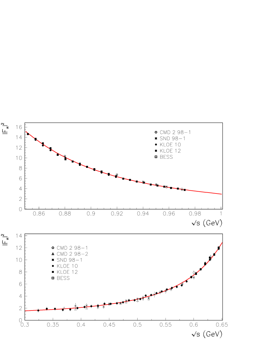
Figure 2: The pion form factor data and fit corresponding to the iteration # 1 BHLS global fit. The $e^{+}e^{-}\rightarrow\pi^{+}\pi^{-}$ data samples are those shown in the entry ”Fit Combination 2” in Table 2. The inset in the top panel magnifies the $\rho^{0}-\omega$ peak region. The dowmost panels magnify the behavior in both distribution wings. See Section 7.2 for further comments.

Therefore, this proves that the scan data from CMD2 and SND are consistent with the KLOE10, KLOE12 and BESSIII data samples and that all these are fully consistent with the other data spectra introduced in the global fit procedure as indicated by the global fit probability. One should also remark that the systematic uncertainties provided for KLOE12 lead to a satisfactory global fit, in contrast with KLOE08, as already noted in the previous Subsection.

Except otherwise stated, the fit parameter values presented from now on are derived using the $e^{+}e^{-}\rightarrow\pi^{+}\pi^{-}$ data samples corresponding to the ”Fit Combination 2” (see Table 2); the fit results are those derived after the first iteration and they do not differ significantly from the corresponding results at iteration # 2. The fit quality for the non–$\pi^{+}\pi^{-}$ data samples are almost undistinguishable from the numbers already given in the second data column from Table 1; they are not repeated for the sake of brevity.

7.3 The Iterative Method : Updating The Model Parameter Values

Beside improving the fits by mean of the iterative method, the present work accounts for an error and a couple of bugs affecting our [34, 35]. Moreover, the present work includes the new KLOE12 data sample within the fit procedure; this is not harmless as KLOE12 constrains the fit conditions more severely than the KLOE10 sample. Therefore, the present results update and supersede the corresponding ones previously given in [34, 35].

7.3.1 The HLS–FKTUY Parameters

The non–anomalous HLS Lagrangian (broken or not) can be written :

$${\cal L}_{HLS}={\cal L}_{A}+a_{HLS}{\cal L}_{V}$$ (12)

The unbroken expression for ${\cal L}_{HLS}$ can be found in [13] and its broken expression (BHLS) is given in [34]. The covariant derivative which allows to construct both pieces of ${\cal L}_{HLS}$ introduces the fundamental parameter $g$, known as universal vector coupling. The coefficient $a_{HLS}$ is a specific feature of the HLS model, expected close to 2 in standard VMD approaches; however, phenomenology rather favors $a_{HLS}\simeq 2.5$ since the early applications of the HLS model to pion form factor studies [77, 78, 23].

On the other hand, the anomalous (FKTUY) sector [15] of the HLS model [13] consists of 5 pieces (see also Appendix D in [34]), each weighted by a specific numerical parameter not fixed by the theory. Using common notations [13, 34] and factoring out, for convenience, the weighting factors, the FKTUY Lagrangian collecting all the anomalous couplings can be written :

$${\cal L}_{FKTUY}=c_{3}{\cal L}_{VVP}+(c_{4}-c_{3}){\cal L}_{AVP}+(1-c_{4}){\cal L}_{AAP}+(c_{1}-c_{2}-c_{3}){\cal L}_{VPPP}+(c_{1}-c_{2}+c_{4}){\cal L}_{APPP}$$ (13)

where $P$ and $V$ indicate the basic pseudoscalar and vector meson nonets and $A$ the electromagnetic field. As ${\cal L}_{HLS}$, ${\cal L}_{FKTUY}$ depends on the universal vector coupling $g$.

At iteration # 1, the global BHLS fit returns :

$$\left\{\begin{array}[]{lll}\displaystyle c_{+}\equiv\frac{(c_{4}+c_{3})}{2}&=~{}~{}~{}0.956\pm 0.004\\[5.69046pt] \displaystyle c_{-}\equiv\frac{(c_{4}-c_{3})}{2}&=-0.166\pm 0.021\\[5.69046pt] \displaystyle c_{1}-c_{2}&=~{}~{}~{}0.915\pm 0.052\\[5.69046pt] \displaystyle g&=~{}~{}~{}5.507\pm 0.001\\[5.69046pt] \displaystyle a_{HLS}&=~{}~{}~{}2.479\pm 0.001\end{array}\right.$$ (14)

with correlation coefficients never larger than the percent level, except for $<\delta g~{}\delta a_{HLS}>=-0.30$ and $<\delta[c_{1}-c_{2}]~{}\delta[(c_{4}-c_{3})/2]>=+0.86$. The sign of the $(g,a_{HLS})$ correlation term is easy to understand as the vector meson coupling to a pion or kaon pair rather depends on the product $g^{\prime}=a_{HLS}g$. The large value of the $([c_{1}-c_{2}],~{}[c_{4}-c_{3}])$ correlation is also not surprising (see footnote 27). The numerical values for $g$ and $a_{HLS}$ are in the usual ball park and do not call for more comments than in [34, 35].

Our value for $c_{+}$ agrees with the estimates derived in [13] from the $\pi^{0}\gamma\gamma^{*}$) form factor ($c_{+}=1.06\pm 0.13$) and from the $\omega\rightarrow\pi^{0}\gamma$ partial width ($c_{+}=0.99\pm 0.16$) with a much smaller uncertainty due to the large amount of data influencing the (global) fit. After the bug fixing, $c_{-}$ is found small but non–zero with a large significance and $(c_{1}-c_{2})$ becomes closer to 1. Using the full $25\times 25$ parameter error covariance matrix returned by the global fit, we have computed separately $c_{4}$ and $c_{3}$ by a Monte–Carlo sampling. This gives $c_{3}=1.124\pm 0.022$ and $c_{4}=0.789\pm 0.021$.

Among the numbers displayed in Eq. (14), some are appealing : The nearness to 1 of the fitted $c_{1}-c_{2}$ and $c_{+}$ parameters, their customary guessed value [13], should be noted and deserves confirmation with more precise data on the anomalous annihilations and light meson radiative decays than those presently available.

7.3.2 The Iterative Method : Pseudoscalar Meson Mixing and Decay Parameters

The BHLS symmetry breaking of the Lagrangian piece ${\cal L}_{A}$ leads to pseudoscalar physical fields constructed as linear combinations of their bare partners. The mechanism involved is the BKY mechanism extended so as to account for both Isospin and SU(3) symmetry breakings [34]; it can be complemented by the pseudoscalar nonet symmetry breaking scheme generated by the t’Hooft determinant terms [79]. The main effect of these determinant terms is to provide the bare Lagrangian with a correction to the PS singlet kinetic energy term governed by a parameter $\lambda$ expected small (see Eq. (7) in [34]).

	General Fit	Constrained Fit
$\theta_{0}$	$2.77^{\circ}\pm 0.41^{\circ}$	0
$\theta_{8}$	$-25.95^{\circ}\pm 0.35^{\circ}$	$-25.52^{\circ}\pm 0.20^{\circ}$
$\theta_{P}$	$-15.29^{\circ}\pm 0.32^{\circ}$	$-13.96^{\circ}\pm 0.16^{\circ}$
$\lambda$	$(2.91\pm 3.35)~{}10^{-2}$	$(1.86\pm 1.17)~{}10^{-2}$
$\varepsilon_{0}$	$(4.12\pm 0.33)~{}10^{-2}$	$(4.00\pm 0.33)~{}10^{-2}$
$\varepsilon(\eta)$	$(5.85\pm 0.48)~{}10^{-2}$	$(5.57\pm 0.47)~{}10^{-2}$
$\varepsilon^{\prime}(\eta^{\prime})$	$(1.46\pm 0.13)~{}10^{-2}$	$(1.36\pm 0.12)~{}10^{-2}$
$\chi^{2}/N_{dof}$	$887.5/994$	$892.5/995$
Probability	99.3%	99.1 %

Table 3: Some parameter values derived when leaving free $\theta_{P}$ and $\lambda$ (first data column) or when relating them by imposing $\theta_{0}=0$ to the fit (second data column).

The BHLS model connects to (Extended) ChPT [25, 24], especially its two angle $\theta_{0}$ and $\theta_{8}$ mixing scheme; in particular, it relates these angles to the singlet–octet mixing angle traditionally denoted $\theta_{P}$, together with the BKY breaking parameters $z_{A}$, $\Delta_{A}$ and to $\lambda$ [34].

The upper part of Table 3 displays in its first data column our fit results in the general case. The fit value for $\theta_{8}$ is in good agreement with other expectations [24] as well as that for $\theta_{0}$. The smallness of this has led us to impose $\theta_{0}=0$ within fits which leads to the results shown in the second data column. The value for $\lambda$ undergoes a severe correction compared with [34, 35] and, presently, because of its large uncertainty, could be neglected without any real degradation in fit qualities.

BHLS also allows for some additional contribution to the $\pi^{0}-\eta-\eta^{\prime}$ mixing based on some possible aspects of Isospin breaking not already accounted for by the extended BKY scheme developped in [34]. This turns out to redefine the physical (observable) fields (right–hand side) in terms of the (BHLS) renormalized (left–hand side) fields by [80] :

$$\left\{\begin{array}[]{lll}\displaystyle\pi_{R}^{3}=\pi^{0}-\varepsilon~{}\eta-\varepsilon^{\prime}~{}\eta^{\prime}\\[14.22636pt] \displaystyle\eta_{R}^{8}=\cos{\theta_{P}}(\eta+\varepsilon~{}\pi^{0})+\sin{\theta_{P}}(\eta^{\prime}+\varepsilon^{\prime}~{}\pi^{0})\\[14.22636pt] \displaystyle\eta_{R}^{0}=-\sin{\theta_{P}}(\eta+\varepsilon~{}\pi^{0})+\cos{\theta_{P}}(\eta^{\prime}+\varepsilon^{\prime}~{}\pi^{0})\end{array}\right.$$ (15)

Inspired by [80], one can lessen the number of free parameters by stating :

$$\left\{\begin{array}[]{ll}\displaystyle\varepsilon=&\displaystyle\epsilon_{0}\cos{\theta_{P}}\frac{\sqrt{2}\cos{\theta_{P}}-\sin{\theta_{P}}}{\sqrt{2}\cos{\theta_{P}}+\sin{\theta_{P}}}\\[14.22636pt] \displaystyle\varepsilon^{\prime}=&\displaystyle-2\epsilon_{0}\sin{\theta_{P}}\frac{\sqrt{2}\cos{\theta_{P}}+\sin{\theta_{P}}}{\sqrt{2}\cos{\theta_{P}}-\sin{\theta_{P}}}\end{array}\right.$$ (16)

and fit $\epsilon_{0}$. Then, using the fit results (parameter central values and error covariance matrix), one can reconstruct the value for $\varepsilon$ and $\varepsilon^{\prime}$. The updated values are given in Table 3 still indicate a $\pi^{0}-\eta$ mixing much larger than the $\pi^{0}-\eta^{\prime}$ mixing (a factor of 4).

Before closing this Subsection, we mention that the Monte Carlo sampling method allows to reconstruct the decay constant ratio $f_{K}/f_{\pi}=1.265\pm 0.009$ which becomes $f_{K}/f_{\pi}=1.295\pm 0.002$ when constraining the fit with $\theta_{0}=0$.

8 The Muon LO–HVP : Evaluations From Iterated Fits

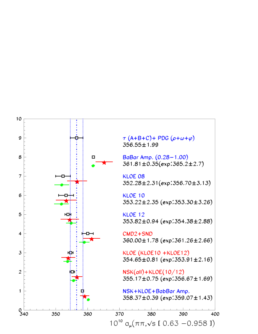
Figure 3: Values for $a_{\mu}(\pi\pi,[0.63,0.958])$ in units of 10^-10 derived from global fits using the indicated $e^{+}e^{-}\rightarrow\pi^{+}\pi^{-}$ data samples or combinations; the $\tau$ dipion spectra are always used. The full green circles are the results obtained from the $A=m$ fit (no iteration) and the black empty squares are the results obtained from the $A=M_{0}$ fit (first iteration). The values derived by integrating the experimental spectra are indicated by red stars. See Subsection 8.1 for comments.

The main aim of the present study is to produce improved estimates of the muon LO–HVP [34, 35] by means of the $iterated$ global fit method expected to cancel out possible biasing effects which could affect the $A=m$ (i.e. non–iterated) solution. The validity of the iterated method is supported by the Monte Carlo study outlined in Appendix A, which clearly indicates that the iterated method cancels out possible biases and returns, correctly estimated, the fit parameter uncertainties. Therefore, building on the conclusions collected in Subsection 4.4 one can produce bias free evaluations of the muon LO–HVP. The effects of iterating from $M_{0}$ to $M_{1}$ – the solution derived using $A=M_{0}$ within the fit procedure – will be especially emphasized. To be complete, this update also takes into account the new KLOE12 [38] and BESSIII [41] $\pi^{+}\pi^{-}$ data samples – which happen to be very constraining – and also corrects for some bugs. Therefore the present numerical results supersede the corresponding ones in [34, 35].

8.1 Various Evaluations Of $a_{\mu}(\pi\pi,[0.63,0.958]~{}$GeV)

The point at top of Figure 3 is the so–called $\tau$+PDG [35] value for $a_{\mu}(\pi\pi,[0.63,0.958]~{}$GeV) derived by switching off the contributions of the various $e^{+}e^{-}\rightarrow\pi^{+}\pi^{-}$ data samples from the minimized $\chi^{2}$, replacing them by decay information extracted from the Review of Particle Properties (RPP) [61] as emphasized in Subsection 7.1.

In order to get the other points displayed in Figure 3, one always uses all the channels covered by BHLS, including the $\tau$ spectra from ALEPH, CLEO and Belle. As for the $e^{+}e^{-}\rightarrow\pi^{+}\pi^{-}$ data samples, one uses each of the BaBar, KLOE08, KLOE10 and KLOE12 samples in isolation as indicated within the Figure (see also Table 2 and Subsection 7.2). The point flagged by CMD2+SND is obtained from a fit to the so–called [34] new timelike data from CMD2 and SND [74, 52, 53, 54], leaving aside the older data from OLYA and CMD collected in [75] (see Table 2 and Section 6 above). As for the BaBar spectrum, for reasons already stated, the fit is performed on the spectrum amputated from the drop off region ($\sqrt{s}\in[0.76,0.80]~{}$ GeV). Finally, as the published BESSIII spectrum ends up at 0.9 GeV, one cannot produce an experimental value on the interval $[0.63,0.958]$ GeV.

As a general statement, Figure 3 clearly illustrates that the iterated ($M_{1}$) and the non–iterated ($M_{0}$) solutions provide quite similar fit estimates for $a_{\mu}(\pi\pi,[0.63,0.958]~{}$GeV). One should nevertheless remark that the agreement between both fit solutions and the numerical integral of the experimental data is less satisfactory for the data samples which exhibit poor fit qualities within the global framework (KLOE08 and BaBar) than for the others (KLOE10, KLOE12, CMD2+SND) as can be inferred from the ”fit in isolation” properties displayed in Table 2. Finally, the weighted averages of the experimental results for KLOE10 and KLOE12 alone or together with all NSK data (the so–called new timelike data and the former samples [75]) are always well reproduced by the global fit and are supported by quite good probabilities (see Table 2).

Using the NSK+KLOE(10/12) sample configuration, the iterated BHLS global fit gives a slightly smaller central value (by $\simeq 1.5~{}10^{-10}$) while the uncertainty is improved by a factor $\simeq 2$. It is also worth pointing out the role of the $\tau$ spectra within the BHLS global fit framework. The following numbers illustrate how the constraints involved by the $\tau$ spectra allow BHLS to yield a more precise fit estimate for $a_{\mu}(\pi\pi,[0.63,0.958]~{}$GeV). Comparing the direct integration result to the values derived from fits, one indeed gets at iteration # 1 :

$$\left\{\begin{array}[]{lll}{\rm Direct~{}Integration{}{}{}{}{}{}}&:&a_{\mu}(\pi\pi,[0.63,0.958])=356.67\pm 1.69\\ A=M_{0}({\rm fit~{}excl.}\tau){}{}{}{}&:&a_{\mu}(\pi\pi,[0.63,0.958])=355.07\pm 0.96\\ A=M_{0}({\rm fit~{}incl.}\tau){}{}{}{}&:&a_{\mu}(\pi\pi,[0.63,0.958])=355.17\pm 0.75\end{array}\right.$$ (17)

in units of $10^{-10}$.

Finally, the downmost point in Figure 3 displays the result derived using all data samples (except for KLOE08 as there is not enough published information to account for its strong correlation with KLOE12); this estimate for $a_{\mu}(\pi\pi,[0.63,0.958])$ which benefits from a very small uncertainty has, however, a poor fit probability as clear from Table 2.

8.2 Contributions To The Muon LO–HVP Up To 1.05 GeV

Channel	$A=m$	$A=M_{0}$	Exp. Value
$\pi^{+}\pi^{-}$	$495.06\pm 1.43$	$494.59\pm 0.89$	$492.98\pm 3.38$
$\pi^{0}\gamma$	$4.53\pm 0.04$	$4.54\pm 0.04$	$3.67\pm 0.11$
$\eta\gamma$	$0.64\pm 0.01$	$0.64\pm 0.01$	$0.56\pm 0.02$
$\pi^{+}\pi^{-}\pi^{0}$	$40.83\pm 0.57$	$40.84\pm 0.57$	$43.54\pm 1.29$
$K_{L}K_{S}$	$11.56\pm 0.08$	$11.53\pm 0.08$	$12.21\pm 0.33$
$K^{+}K^{-}$	$16.79\pm 0.20$	$16.90\pm 0.20$	$17.72\pm 0.52$
Total	$569.41\pm 1.55$	$569.04\pm 1.08$	$570.68\pm 3.67$

Table 4: The contributions to the muon LO–HVP from the various channels covered by BHLS from their respective thresholds to 1.05 GeV in units of $10^{-10}$ at start and after iteration. The last column displays the direct numerical integration of the various spectra used within BHLS. The $\pi^{+}\pi^{-}$ data samples considered are those flagged by ”Combination 2” in Table 2.

The LO–HVP’s integrated from their respective thresholds up to 1.05 GeV are displayed in Table 4; the central value for $a_{\mu}(\pi\pi)$ includes final state radiation (FSR) effects. The first data column shows the results from the fit solution $M_{0}$ derived from fitting with $A=m$; the second data column displays the results corresponding to the solution $M_{1}$ derived by fitting with $A=M_{0}$. These two data columns report on the fits performed using all annhilation channels encompassed by BHLS $and$ the $\tau$ dipion spectra. Finally, the rightmost data column provides the direct numerical integration of the experimental spectra – actually only those feeding the BHLS fit procedure, including the KLOE10, KLOE12 and BESSIII data samples besides the scan data.

As for the $\pi^{+}\pi^{-}$ channel, both fits – which include the $\tau$ spectra – provide central values in agreement with each other and with the direct estimate within the quoted error. If the $A=m$ solution were (inherently) exhibiting a bias, comparing the first two numbers in the first line of Table 4 indicates that this does not exceed $\simeq 0.5\times 10^{-10}$ – e.g. half a standard deviation. Therefore, real experimental data samples confirm the gain provided by a global fit procedure when samples with normalization errors small compared to their statistical accuracies are included; exploring this effect is the purpose of Subsection A.2.3 in Appendix A.

One should also remark that the unbiasing iterative procedure lessens significantly the uncertainty on $a_{\mu}(\pi^{+}\pi^{-})$ compared with the $A=m$ solution and, over the whole range of validity of BHLS (up to 1.05 GeV), one ends up with a factor of $\simeq$ 3 reduction of the uncertainty compared to the direct numerical integration. The same kind of effect is reported in [47] concerning the spread of the parton density functions.

Therefore, relying on the iterative procedure, one observes that the global fit does not produce significant shifts of the central values of the HVP contributions which could be attributed to the normalization (scale) uncertainties strongly affecting some data samples. Relying on the Monte Carlo studies outlined in Appendix A, this can be attributed to the large number of data samples where the statistical uncertainties dominate over the normalization uncertainty. Moreover, the uncertainty on the part of the LO–HVP derived from the BHLS fit (more than 80% of the total LO–HVP) is very small and even marginal.

8.3 The Muon $g-2$ From BHLS Global Fit Procedure

Contribution from	Energy Range	LO–HVP (2014)	LO–HVP (2011)
missing channels	threshold $\to$ 1.05	$1.34(0.03)(0.11)[0.11]$	$1.44(0.40)(0.40)[0.57]$
$J/\psi$		$8.94(0.42)(0.41)[0.59]$	$8.51(0.40)(0.38)[0.55]$
$\Upsilon$		$0.11(0.00)(0.01)[0.01]$	$0.10(0.00)(0.01)[0.01]$
hadronic	(1.05, 2.00)	$60.45(0.21)(2.80)[2.80]$	$60.76(0.22)(3.93)[3.94]$
hadronic	(2.00, 3.10)	$21.63(0.12)(0.92)[0.93]$	$21.63(0.12)(0.92)[0.93]$
hadronic	(3.10, 3.60)	$3.77(0.03)(0.10)[0.10]$	$3.77(0.03)(0.10)[0.10]$
hadronic	(3.60, 5.20)	$7.50(0.04)(0.05)[0.06]$	$7.64(0.04)(0.05)[0.06]$
pQCD	(5.20, 9.46)	$6.27(0.00)(0.01)[0.01]$	$6.19(0.00)(0.00)[0.00]$
hadronic	(9.46, 13.00)	$1.28(0.01)(0.07)[0.07]$	$1.28(0.01)(0.07)[0.07]$
pQCD	(13.00,$\infty$)	$1.53(0.00)(0.00)[0.00]$	$1.53(0.00)(0.00)[0.00]$
Total	1.05 $\to\infty$	$112.82\pm 3.01_{tot}$	$112.96\pm 4.13_{tot}$
	+ missing channels

Table 5: LO–HVP contributions to $10^{10}a_{\mu}$ with FSR corrections included. The statistical and systematic errors are given within brackets; the total uncertainty is given within square brackets. Column ”LO–HVP (2011)” displays the contributions estimated using only the data samples available in 2011; Column ”LO–HVP (2014)” displays the corresponding values updated with the data samples published up to the end of 2014.

In order to evaluate the muon LO–HVP from the fit results derived by means of the BHLS global fit procedure, the numbers given in Table 4 should be supplied with several additional contributions which cannot be derived from within the BHLS framework but should be estimated by other means. This covers the channels opened below 1.05 GeV but remaining outside the present BHLS scope and, more importantly, all hadronic contributions covering the non–perturbative QCD region above 1.05 GeV should be estimated via the direct integration method.

Table 5 summarizes these additional contributions to be combined with the BHLS results to derive the muon LO–HVP; in this Table, one reminds the information available by end of 2011 and used in our previous [34, 35]. The data column flagged by ”LO–HVP (2014)” is the update derived by taking into account the data samples more recently collected (and published up to the end of 2014); these are the $e^{+}e^{-}\to 3(\pi^{+}\pi^{-})$ data from CMD–3 [81], the $e^{+}e^{-}\to\omega\pi^{0}\to\pi^{0}\pi^{0}\gamma$ from SND [82] and several data samples collected by BaBar in the ISR mode [83, 84, 85, 86]. These data samples highly increase the available statistics for the annihilation channels opened above 1.05 GeV and lead to significant improvements. One thus should note the important improvement these provide for the LO–HVP contribution from the $[1.05,~{}2.0]$ GeV region : its uncertainty is reduced by 25 %, while its central value is almost unchanged. Despite this improvement, the energy region $[1.05,~{}2.0]$ GeV still remains the dominant uncertainty on the muon LO–HVP and this strongly limits the effect of gaining further in precision on the part of the LO–HVP covered by BHLS.

Deriving the full HVP value also requires to account for the higher order effets. This includes the next–to–leading order contribution (NLO) taken from [26] ($[-9.97\pm 0.09]\times 10^{-10}$) and the recently estimated next–to–next–to–leading order (NNLO) effects which happen to be non–negligible ($[1.24\pm 0.01]\times 10^{-10}$) [87].

To compute the muon $g-2$, one should also include the light–by–light (LBL) contribution (here taken from [88]), the QED contribution [89, 90] and the electroweak contribution (EW) [31]. The next–to–leading order contribution to the LBL amplitude (NLO–LBL) has also been computed recently [91] but is clearly negligible ($[0.3\pm 0.2]\times 10^{-10}$). Altogether, the numerical values we use (see Table 6) are rather consensual [92].

$10^{10}\times a_{\mu}$	Values (incl. $\tau$)		Direct Integration
	scan only	scan $\oplus$ KLOE $\oplus$ BESSIII	scan $\oplus$ KLOE $\oplus$ BESSIII
LO–HVP	$683.26\pm 3.78$	$681.86\pm 3.20$	$683.50\pm 4.75$
HO (NLO) HVP	$-9.97\pm 0.09$   [26]
NNLO HVP	$~{}1.24\pm 0.01$   [87]
LBL	$10.5\pm 2.6$   [88]
NLO–LBL	$0.3\pm 0.2$   [91]
QED	$11~{}658~{}471.8851\pm 0.0036$   [89, 90]
EW	$15.40\pm 0.10_{\rm had}\pm 0.03_{\rm Higgs,top,3-loop}$   [31]
Total Theor.	$11~{}659~{}172.62\pm 4.60$	$11~{}659~{}171.22\pm 4.13$	$11~{}659~{}172.86\pm 5.42$
Exper. Aver.	$11~{}659~{}208.9\pm 6.3$
$\Delta a_{\mu}$	$36.28\pm 7.80$	$37.68\pm 7.53$	$36.04\pm 8.31$
Significance ($n\sigma$)	$4.65\sigma$	$5.00\sigma$	$4.38\sigma$

Table 6: The various contributions to $10^{10}a_{\mu}$. $\Delta a_{\mu}=a_{\mu}^{exp}-a_{\mu}^{th}$ is given in units of $10^{-10}$. For the measured value $a_{\mu}^{exp}$, we have adopted the value reported in the RPP which uses the updated value for $\lambda=\mu_{\mu}/\mu_{p}$ recommended by the CODATA group [93]. By KLOE, one means that the KLOE10 and KLOE12 $\pi^{+}\pi^{-}$ data samples are introduced in the BHLS fit procedure $and$ in the directly integrated spectra.

The first data column in Table 6 reproduces (after our methodological update) the muon anomalous moment estimate coming from the corresponding BHLS global fit where only the scan data for the $\pi^{+}\pi^{-}$ channel are considered while all ISR data are excluded. This supersedes the corresponding information in [34]. The sample combination preferred by the BHLS global fit gives the results displayed in the second data column; it exhibits a $4.9\sigma$ significance for a non–zero $\Delta a_{\mu}=a_{\mu}^{exp}-a_{\mu}^{th}$. The evaluation derived by direct integration of the spectra used within the global fits are given in the third data column. The new data, as a whole, increase the discrepancy for $\Delta a_{\mu}$ which is always found above the $4\sigma$ level; effects of additional and not still accounted for systematics will be examined in the next Subsection.

Figure 4 displays the results for $\Delta a_{\mu}$ derived using or not the $\tau$ data and various combinations of the available $\pi^{+}\pi^{-}$ data samples introduced within the BHLS global fit procedure at first iteration. For comparison, one also displays in this Figure the evaluations produced by other authors and flagged by Dhea09 [29], DHMZ10 [58], JS11 [26] and HLMNT11 [60] – corrected however for the recently calculated NNLO–HVP and NLO–LBL – contributions as included in Table 6. A priori, the Dhea09 estimate compares exactly to our evaluations using scan data only; the other results are derived using, beside the NSK samples, the BaBar, KLOE08 and KLOE10 samples. These may compare to the last couple of lines in Figure 4 where the scan data are supplemented with the BaBar (not truncated), KLOE (10/12) and BESSIII samples.

The following comments are in order here :

• 1/ The difference between our estimates and those of other authors mainly concerns the estimated central value for $\Delta a_{\mu}$. Also, our uncertainties are now reduced because of the global fit method, but also because of using much more data samples than other authors; this is clear by comparing the errors shown in Figure 4 with those given in [35].

  When using only the scan data, the shift one observes should reflect the biasing effect certainly present in the experimental data (see footnote # 29) and corrected in our approach by the iterated fit method. When the ISR $\pi^{+}\pi^{-}$ samples are also involved, the issue just reminded is amplified because the weight of samples with large overall scale uncertainties is much increased. The effect of the BaBar data sample is no longer enough to balance the effect of the new data samples as clear by comparing the lines for ”NSK+KLOE+BESSIII” with the lines for ”Global (ISR+scan)” which also include the (full) BaBar sample. Nevertheless, one should note the large difference of the correponding probabilities.

• 2/ When a comparison between a $\Delta a_{\mu}$ estimate derived using the $\tau$ data and the corresponding one excluding these is possible, ours exhibits the smallest difference ($1.12\times 10^{-10}$ for NSK+KLOE+BESSIII, $-0.7\times 10^{-10}$ for the Global fit including all the $\pi^{+}\pi^{-}$ data samples). This is certainly due to the vector meson mixing which defines the BHLS model. It is interesting to note that the JS11 [26] value, which is based on the $\gamma-\rho^{0}$ mixing by loop transitions, is the closest to ours.

• 3/ Relying on the global fit properties, the BHLS model favors the ”NSK + KLOE10 + KLOE12 +BESSIII + $\tau$” as the largest consistent set of data samples. This leads to $\Delta a_{\mu}=(37.55\pm 4.12)\times 10^{-10}$ which exhibits a $5.\sigma$ significance. Our estimate is expected to be free of biases generated by the overall scale uncertainties which dominate the ISR $\pi^{+}\pi^{-}$ data samples.

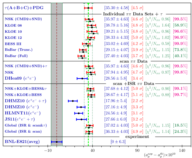
Figure 4: The deviation $\Delta a_{\mu}=a_{\mu}^{exp}-a_{\mu}^{th}$ in units of 10^-10. The various $a_{\mu}^{th}$ have been derived from the global fit using the indicated $e^{+}e^{-}\rightarrow\pi^{+}\pi^{-}$ data samples and including/excluding the $\tau$ dipion spectra as indicated. In red we display $\Delta a_{\mu}$ corresponding to the iterated solution and in green those corresponding to the $A=m$ (non–iterated) solution. In blue results from other studies are given corrected by the recently evaluated next–to–next–to–leading order contribution [87]. See Section 8.3 for comments.

8.4 Additional Systematics On The BHLS Estimate For The Muon $g-2$

A detailed study of additional systematics possibly affecting the BHLS evaluation of $\Delta a_{\mu}$ has been already performed in [35]. It concluded to an uncertainty of the LO–HVP central value for $\Delta a_{\mu}=a_{\mu}^{exp}-a_{\mu}^{th}$ in the range $[-1.3\div 0.60]\times 10^{-10}$ coming from $\pi^{+}\pi^{-}$ contribution in the $\phi$ mass region, where BHLS is weakly constrained. An uncertainty coming from using the $\tau$ spectra has also been considered; it was argued that the best motivated evaluation of this is the difference between fitting with the $\tau$ spectra and without them in the most constrained configuration. Presently, this means that the BHLS preferred value ($\Delta a_{\mu}=(38.58\pm 5.04)\times 10^{-10}$) could be underestimated by $\simeq 0.9\times 10^{-10}$.

Another mean to detect systematics is to compare with the accurate ChPT predictions on the $P$–wave $\pi^{+}\pi^{-}$ phase–shift [94] and also with the available experimental data from the Cern–Munich [95] and Fermilab [96] groups. These are shown in Figure 5. Included also are the predictions derived from the Roy Equations [97] and from the phase of the pion form factor fit performed in [26] (JS11).

As for the BHLS predictions corresponding to using NSK+KLOE(10/12), we display in this Figure the phase of the full amplitude and those corresponding to dropping out the isospin breaking (IB) effects due to the vector meson mixing. The $\tau$ spectra are included within the fit procedure.

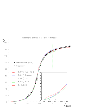
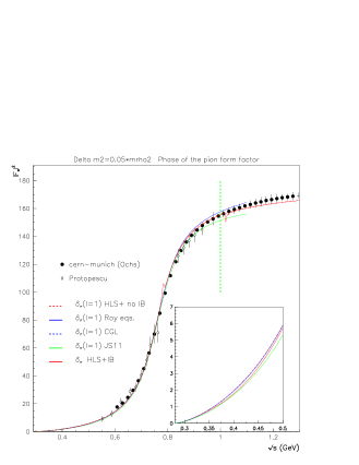
Figure 5: $P$–wave $\pi^{+}\pi^{-}$ phase–shift data and predictions from [94] (CGL) and [26] (JS11) together with the BHLS phase–shift. The insets magnify the various behaviors close to threshold. See Subsection 8.4 for further explanations.

The standard BHLS phase shift predictions are displayed in the left–hand side panel of Figure 5. One clearly observes a very good prediction of the phase–shift up to about 1.2 GeV, i.e. much beyond our fitting range (from threshold to 1.0 GeV for the $\pi\pi$ data). Indeed the Cern–Munich data are very well accounted for and the BHLS predictions are in accord with the other predictions. The inset, however, exhibits a (minor) issue for the full amplitude phase, a small bump of about $1^{\circ}$ close to threshold, absent from the IB amputated amplitude. This can be tracked back to a peculiarity of the broken HLS model which does not split up the HK (Lagrangian) masses for the $\omega$ and $\rho^{0}$ mesons and, consequently, the mixing angle $\alpha(s)$ does not exactly vanish at $s=0$ (see Figure 6 in [32]); in contrast the other angles fulfill $\beta(0)=\gamma(0)=0$. Indeed, one has :

$$\alpha(s)=\frac{\epsilon_{1}(s)}{[m_{\rho}^{HK}]^{2}-[m_{\omega}^{HK}]^{2}+\Pi_{\pi\pi}(s)}$$ (18)

where [34] $\epsilon_{1}(s)$ is the difference of the charged and neutral kaon loops and $\Pi_{\pi\pi}(s)$ is the pion loop which both vanish at $s=0$. This assumption has been checked with fits by imposing $[m_{\omega}^{HK}]^{2}=(1+\eta)[m_{\rho}^{HK}]^{2}$ and choosing various fixed values for $\eta$; the right–hand side panel in Figure 5 displays the phase shift for $\eta=5\%$ and, quite satisfactorily, its inset does not reveal a bump any longer. A non–zero (HK) mass difference $\eta~{}[m_{\rho}^{HK}]^{2}$ cannot be generated by the breaking mechanisms already implemented within BHLS. However, a breaking of the nonet symmetry in the vector meson sector (VNSB) enables such an effect; this turns out to modify the customary vector field matrix – actually U(3) symmetric – within the covariant derivatives of the HLS model [13] by a perturbation term proportional to the singlet vector field combination. The effect of VNSB has been derived from specific fit studies and indicates that $\Delta a_{\mu}$ might have to be lessened by about $1.4\times 10^{-10}$.

Therefore, in total, the BHLS favored result can be expressed, in units of $10^{-10}$ as :

$$\Delta a_{\mu}=37.68+[^{+0.6}_{-1.3}]_{\phi}+[^{+0.9}_{-0.0}]_{\tau}+[^{+0.0}_{-1.4}]_{VNSB}\pm 4.12_{th}\pm 6.3_{exp}$$ (19)

where the three additional contributions play as shifts on the central value. Adding them up linearly, the maximum shift ($-2.7\times 10^{-10}$) may reduce the central value to $34.85\times 10^{-10}$ which has still a $4.6\sigma$ significance. The effect of these additional systematics is to reduce potentially by $\simeq 0.3\sigma$ all the significances displayed in Figure 4. These are not due to overall scale uncertainties already accounted for by the iterative method; they might be reduced by new annihilation data samples covering the region up to 1.05 GeV in all the physics channels in the realm of BHLS.

8.5 The HVP Slope At Origin In BHLS Fits

In the lattice QCD approach of calculating $a_{\mu}^{\rm had}$, extrapolation methods have been developed (see e.g. contributions to [98]) to overcome difficulties to reach the physical point in the space of extrapolations. The low $Q^{2}$ behavior of the euclidian electromagnetic current correlators on a lattice, which exhibits a discrete momentum spectrum, poses a particular challenge (see e.g. [99, 100] and References just below). The analysis of moments of the subtracted photon vacuum polarization function $\Pi(Q^{2})$ was particularly advocated in variants in Refs. [101] and [102]. Recent lattice calculations [103, 104, 105, 106] have been utilizing moment analysis techniques for a more precise evaluation of $a_{\mu}^{\rm had}$. The leading moment is given by the slope of the Adler function [107, 108], the latter being given by :

$$D(Q^{2})=Q^{2}\>\left[\int_{s_{min}}^{\infty}\frac{R(s)}{(s+Q^{2})^{2}}{\rm d}s\>\right]=\frac{3\pi}{\alpha}Q^{2}\frac{d}{dQ^{2}}\Delta\alpha_{\mathrm{had}}(-Q^{2})$$ (20)

where $R(s)$ is the hadronic spectral function and $s_{min}$ the smallest threshold energy squared ($s_{min}=m_{\pi^{0}}^{2}$ within BHLS). Then, defining :

$$P_{1}=\int_{s_{min}}^{\infty}\,\frac{R(s)}{s^{2}}\,ds~{}~{}~{}~{},$$ (21)

the HVP slope at the origin is given by :

$$\left.\frac{d}{ds}\,\Delta\alpha_{\mathrm{had}}(s)\right|_{-s\to+0}=-\frac{\alpha}{3\pi}\,\int_{s_{min}}^{\infty}\,\frac{R(s)}{s^{2}}\,ds=-\frac{\alpha}{3\pi}P_{1}$$ (22)

The constant $P_{1}$ can be directly estimated from data and partly from the BHLS fits. Therefore, one can proceed as done above with our evaluations of $a_{\mu}^{\rm had}$ and derive the results gathered in Table 7. Here, one observes that the difference between the experimental and the HLS values for the HVP slope are at the percent level (a $2~{}\sigma_{exp}$ effect) and the uncertainty is scaled down by a factor of 10. However, to really feel the HLS improvement on the slope, one needs once more an improved hadronic spectral function at high energies.

moment	data direct	HLS channels data	HLS model	HLS + non HLS
$P_{1}$ (GeV-2)	11.83$\pm$ 0.08	10.07$\pm$ 0.05	9.970$\pm$ 0.016	11.73 $\pm$ 0.06
$\displaystyle 10^{2}\frac{d\Delta\alpha_{\mathrm{had}}}{{\rm d}s}(0)$	$-0.92\pm 0.01$	$-0.78\pm 0.01$	$-0.772\pm 0.001$	$-0.907\pm$ 0.01

Table 7: The slope of the photon HVP at $s=0$.

A lattice estimate of the Adler function slope $D^{\prime}(0)$ has been presented in [109]. The result is ${P}_{1}=5.8(5)~{}\rm GeV^{-2}$, and has been compared with ${P}_{1}=9.81(30)~{}\rm GeV^{-2}$, a result estimated using a phenomenological toy-model representation [110] of the isovector spectral function. The lattice results too include the isovector part only and is missing higher energy contributions above 1 GeV.

In the study [102], the authors provide numerical values from fits to Lattice data based on Padé approximants (PA). For this purpose, they parametrize the HVP as :

$$\Pi(Q^{2})=\Pi(0)-Q^{2}\left[a_{0}+\sum_{n=1}^{N}\frac{a_{n}}{b_{n}+Q^{2}}\right]$$ (23)

which thus leads to  :

$$\frac{d\Delta\alpha_{\mathrm{had}}}{{\rm d}Q^{2}}(0)=4\pi\alpha\frac{d\Pi}{{\rm d}Q^{2}}(0)=-4\pi\alpha\left[a_{0}+\sum_{n=1}^{N}\frac{a_{n}}{b_{n}}\right]$$ (24)

The parameters corresponding to the results they consider as optimal are given in their Table 3. Using their notations, their fitted parameter values lead, for instance, to $(0.71\pm 0.15)\times 10^{-2}$ (PA solution [0,1]) or $(0.75\pm 0.30)\times 10^{-2}$ (PA solution [1,1]). These compare reasonably well to the slope results reported in Table 7 just above, taking into account the proviso expressed above about lattice data.

9 Concluding Remarks

The present study was motivated by the question which gives its title to this paper. More precisely, the issue is whether the D’Agostini bias [42, 46] prevents to derive unbiased physical results from global fits to experimental spectra affected by dominant overall scale uncertainties.

Actually, several issues are merged together. First, the effective global $\chi^{2}$ functions to be used in the minimization procedure should be appropriately defined. For the data samples where the statistical errors dominate the overall scale uncertainties, the construction of the associated partial $\chi^{2}$’s is quite standard. The real issue starts when the data samples are dominated by overall scale uncertainties. For each of them, substantially, the canonical partial $\chi^{2}$ has been reminded in Section 2 and writes [42, 45, 46] :

$$\chi^{2}=[m-M(\vec{a})-\lambda A]^{T}V^{-1}[m-M(\vec{a})-\lambda A],$$

leaving aside the so–called ”penalty term” [46] proportional to $\lambda^{2}$. The (partial) $\chi^{2}$ being appropriately defined, another issue is the choice of the vector $A$.

In our former studies [34, 35], beside the $\simeq 40$ data samples dominated by statistical errors which follow the traditional treatment, the data samples covering the $e^{+}e^{-}\rightarrow\pi^{+}\pi^{-}$ annihilation channel are all, sometime very strongly, dominated by overall scale uncertainties; this especially refers to the samples collected by the KLOE and BaBar Collaborations using the ISR production mode. Here, for each sample, we chose for $A$ the experimental spectrum itself; this choice has been referred to as $A=m$ all along the paper. The guess behind was that all scale uncertainties affecting the different experimental spectra independently of each other should smear out possible biases in the central values of the (common) theoretical form factor function parameters [35].

It happens that the results one can derive in this way from the BHLS global fit undergo very small biases (compared to the errors derived from the fit procedure); this is shown in the present study. However, the guess just reminded was incorrect and the actual reason which explains the almost bias free results is following : As shown in the Monte Carlo study presented in the Appendix, there is no smearing out of biases if $all$ the spectra submitted to fit undergo comparable strong scale uncertainties; however, this study also shows that, if some of the fitted spectra are dominated by (random) statistical errors rather than global scale uncertainties, the fit results can be strongly unbiased.

Nevertheless, a high level of unbiasing cannot be taken as granted as the real weight of the samples dominated by statistical errors within the full global fit procedure cannot be ascertained beforehand. Basically, the choice $A=m$ potentially leads to biases of unknown magnitude; this has been shown by G. D’Agostini [42] with a simple example and more generally argued by V. Blobel [46]. These authors also showed that all biases vanish if, instead of $A=m$, one makes the choice $A=M$, the ”true” spectrum. But this is just not possible within contexts like ours, where fits are performed just in order to derive the ”true” spectrum from data. Fortunately, iterative methods allow to circumvent this difficulty by taking the path opened in [47] in order to derive the parton density function from data and correct for biases. The iterative method we propose has been tested with the Monte Carlo study reported in the Appendix and shown to produce unbiased results with a quite fast convergence speed; indeed, only one iteration is sufficient.

So, our main conclusion is indeed that global fit methods including a fast iterative procedure are expected to produce reliable pieces of information as, methodologically, the central values are unbiased and the estimate for the uncertainties reliable; this especially applies to the part of the muon leading order HVP derived from $e^{+}e^{-}$ annihilation cross sections.

Having shown that appropriate global fit methods should lead to results which can be trusted, a related remark is worth being expressed. Iterative global fits allow to supply the BHLS Effective Lagrangian cross sections with reliable and unbiased numerical central values for the fit parameters and a good estimate of their error covariance matrix. Then, using these cross sections and the fit information, Eq. (1) is expected to provide an unbiased estimate for $a_{\mu}(\pi\pi)$ as the ingredients are unbiased.

On the other hand, when computing $a_{\mu}(\pi\pi)$ by directly integrating a dipion spectrum in order to derive its so–called experimental value, one has to plug into Eq. (1) the experimentally measured cross section $\sigma_{exp.}(s)$. However, as already noted in footnote # 29, or as can be inferred from the canonical $\chi^{2}$ expression reminded just above, the experimental and model cross sections are related by :

$$\sigma_{exp.}(s)=\sigma_{theor.}(s)+\delta\sigma(s)$$

where the best estimate of the second term writes $\delta\sigma(s)=\lambda\sigma_{theor.}(s)$. As obvious from Eq. (6), the best estimate of the scale factor $\lambda$ equally depends on the measured spectrum and on the ”true” spectrum, which can be identified with its (iterated) fit solution. So, using again self–explanatory notations, Eq. (1) leads to :

$$a_{\mu}(\pi\pi,exp.)=a_{\mu}(\pi\pi,theor.)+\delta a_{\mu}(\pi\pi)$$

and thus $a_{\mu}(\pi\pi,exp.)$ looks intrinsically biased for any sample subject to strong enough overall scale uncertainties. This issue is also reflected by the residual plots which are improved when plotting the corrected residuals $[m-(1+\lambda)M(\vec{a})]$ instead of the raw ones $[m-M(\vec{a})]$, as can be seen in Figure 13 of [35]; this allows to infer that $\delta a_{\mu}(\pi\pi)$ is small but non–zero. It amounts to $\delta a_{\mu}(\pi\pi)\simeq 2\times 10^{-10}$ in the case ”NSK+KLOE10+KLOE12+BESSIII+$\tau$” favored by the BHLS model.

As for the physics conclusions, the present paper updates and corrects the results derived by the global BHLS fit method which, following the considerings just summarized, has been completed with an iteration procedure in order to cancel out possible biases. One thus confirms that almost all of the existing data samples covering the annihilation channels with the $\pi^{0}\gamma$, $\eta\gamma$, $\pi^{+}\pi^{-}\pi^{0}$, $K^{+}K^{-}$, $K^{0}\overline{K^{0}}$ final states and the dipion spectra in the $\tau^{\pm}\rightarrow\pi^{\pm}\pi^{0}\nu$ decay accomodate perfectly the BHLS framework. In the line of our previous works, one also finds that among the data samples covering the $e^{+}e^{-}\rightarrow\pi^{+}\pi^{-}$ annihilation, the data samples provided by CMD2 and SND, the KLOE10 and now also the KLOE12 and BESSIII samples behave consistently with each other and with the other considered data covering the various channels entering the BHLS scope.

The present update, which also includes the recently published KLOE12 and BESSIII $\pi^{+}\pi^{-}$ samples, supersedes our previous results; these are mostly given in Table 3 and in Eqs. (14). From a theoretical point of view, it is interesting to note the corrected values for the $c_{i}$’s coefficients of the anomalous (FKTUY) terms of the HLS model [15, 13] : The combinations $c_{+}=(c_{4}+c_{3})/2$ and $c_{1}-c_{2}$ are found very close to the usually assumed value, i.e. 1; in contrast, $c_{-}=(c_{4}-c_{3})/2=-0.166\pm 0.021$ is non–zero with a $8\sigma$ significance.

Figure 3 displays the values for $a_{\mu}(\pi\pi,[0.63,0.958])~{}$GeV derived from iterating the fits with the various available data samples. One observes a strong reduction of the uncertainty compared to the corresponding experimental value (about a factor of 2.5) and there is a close agreement between central values for all samples (or combinations of samples) which yield a good fit probability. The difference between the central values for the starting fit and the iterated one tends to indicate that biases are limited; this should be a consequence of also dealing with a large number of samples where the overall scale uncertainties are dominated by random statistical errors, as argued in the Appendix.

Figure 4 exhibits the values for the muon $\Delta a_{\mu}=a_{\mu}^{exp}-a_{\mu}^{th}$ when various combinations of $e^{+}e^{-}\rightarrow\pi^{+}\pi^{-}$ and $\tau^{\pm}\rightarrow\pi^{\pm}\pi^{0}\nu$ samples are used in the iterated global fit procedure. The present study confirms that, within BHLS and because of its specific isospin breaking mechanisms, one does not observe any serious mismatch between fits with only $e^{+}e^{-}$ annihilation data and fits where these are supplemented with the $\tau$ dipion spectra. The central values for $a_{\mu}(e^{+}e^{-})$ and $a_{\mu}(e^{+}e^{-}+\tau)$ only differ by 2 units (NKS), 1 unit (NSK+KLOE+BESSIII+$\tau$) or 0.7 unit in the global fit of all data samples (including BaBar) as can be seen in Figure 4.

Figure 4 displays the value for $\Delta a_{\mu}$ derived using $all$ data samples except for KLOE08, which can be written :

$$\Delta a_{\mu}=37.02+[^{+0.6}_{-1.3}]_{\phi}+[^{+0.9}_{-0.0}]_{\tau}+[^{+0.0}_{-1.4}]_{VNSB}\pm 4.03_{th}\pm 6.3_{exp},$$

where an estimate of the magnitude of possible uncertainties coming from outside the BHLS framework is proposed. This exhibits a $5\sigma$ significance (which may reduce to $4.6\sigma$ – in the least favorable case – if the additional systematics are added linearly and assumed to play as a shift). One should note however that the fit probability is poor.

The most probable value for the muon $\Delta a_{\mu}$ is obtained by using the CMD2, SND, KLOE10, KLOE12 and BESSIII samples – and the $\tau$ spectra; this leads to :

$$\Delta a_{\mu}=37.68+[^{+0.6}_{-1.3}]_{\phi}+[^{+0.9}_{-0.0}]_{\tau}+[^{+0.0}_{-1.4}]_{VNSB}\pm 4.12_{th}\pm 6.3_{exp}.$$

This BHLS preferred estimate exhibits a $5.\sigma$ significance for a non–zero $\Delta a_{\mu}$, which may reduce to $4.7\sigma$ if one takes into account, as just above, the possible additional systematics. This solution is associated with a 99% fit probability.

As a summary, even complemented with an iterative procedure shown in the Appendix to remove biases, the BHLS approach favors a significance for $\Delta a_{\mu}$ above the $\simeq 4.5\sigma$ level; this value is a lower bound obtained by including possible additional systematics added linearly. New data expected soon may further clarify the picture. The uncertainties now become sharply dominated by the region above 1.05 GeV, i.e. outside the BHLS scope.

Appendix A Appendix : Monte Carlo Tests of the Iterative Procedure

A.1 The Test Method

In order to test the iterative method, one has developped a minimization code which deals with spectra generated from a given underlying function $M_{true}(s)$ where the parameters $\{a_{i}\}$ (which, of course, are known at the generation level) are fitted within the code. The ”experimental” spectra feeding this code are generated using the true distribution smeared by introducing $gaussian$ uncertainty distributions. Indeed, for the purpose of testing our analysis method, it is certainly the most appropriate to rely on ”perfect” data samples, with perfectly known properties.

For sake of simplicity, at the generation level, any ”experimental” spectrum $E$ is chosen to carry 100 ”measurements” $m_{i}^{E}$, performed at 100 equally spaced energy squared $s_{i}$ points ($s_{i}\in[0,~{}1]$ GeV²), the same sequence for all spectra. The ”measurements” are derived by smearing the theoretical values $M_{true}(s_{i})$ in the following way : For each spectrum $E$, one assumes the ”measurements” are sampled out from gaussian distributions in the following way :

$$m_{i}^{E}=M_{true}(s_{i})[1+\sigma\varepsilon_{scale}^{E}(0,1)+\eta\varepsilon_{stat}^{i,E}(0,1)]~{}~{}~{}~{},~{}~{}~{}i=1,\cdots,100$$ (25)

where $\varepsilon_{stat}^{i,E}(0,1)$ indicates the $i^{th}$ sampling on a gaussian distribution of $0$ mean and unit standard deviation generating the statistical error; it varies independently from ”measurement” to ”measurement” and from spectrum to spectrum. $\eta M_{true}(s_{i})$ denotes the statistical error common to all $m_{i}$, $\eta$ being some fixed fraction of the order of a few percents, chosen the same for all the ”measurements” in the spectrum $E$.

On the other hand, $\lambda_{E}=\sigma\varepsilon_{scale}^{E}(0,1)$ is the scale uncertainty affecting specifically the spectrum $E$; as indicated by its definition, it is sampled out from a gaussian distribution of zero mean and $\sigma$ standard deviation. The overall scale uncertainty affecting $E$ is obtained via $one$ sampling of $\varepsilon_{scale}^{E}(0,1)$ which, thus, carries the same value for all the ”measurements” $m_{i}^{E}$ in the spectrum $E$. Of course, when going from a spectrum $E$ to another $E^{\prime}$, another sampling of $\varepsilon_{scale}^{E}(0,1)$ should be performed. For specific tests, the overall scale uncertainty can be switched off ($\sigma=0$).

One defines $N_{rep}$ replicas (generally 1000) of $N_{exp}$ (generally 5) experimental spectra constructed as shown in Eq. (25) and submitted to a global fit where the parameters entering $M_{true}(s)$ are just the parameters to be derived from the fit. The ”true” statistical error covariance matrix $V_{ij}=[\eta M_{true}(s_{i})]^{2}\delta_{ij}$ is practically approximated by $V_{ij}=[\eta m_{i}^{E}]^{2}\delta_{ij}$; we have avoided the unessential complication of non–diagonal covariance matrix. The fit results derived for each replica are stored and then used to construct the statistical plots – true residuals and pulls –with the help of the known parameter ”true” values.

Therefore, we are just in the conditions described in Subsection 4.2. One should note that the minuit code we have built performs the minimization of the $N_{exp}$ samples $and$ runs sequentially to treat the $N_{rep}$ replicas within the same job.

So, for each replica, the global $\chi^{2}$ minimized by our Monte Carlo minuit procedure is simply a sum of $N_{exp}$ terms like Eq. (4):

$$\chi^{2}=\sum_{E=1}^{E=N_{exp}}\chi^{2}_{E}$$ (26)

When initializing the iteration procedure, one uses $A_{E}=m_{E}$, i.e. the spectrum $E$ serves to construct its $\chi^{2}_{E}$; so $A_{E}$ differs from some other $A_{E^{\prime}}$ by statistical fluctuations. When iterating, at first or higher order, they become identical as $A_{E}=A_{E^{\prime}}=M_{fit}\simeq M(\vec{a}_{fit})$.

Obviously, each such run provides simultaneously all the information allowing to examine the statistical properties of the iterative method corresponding to a given theoretical choice $M_{true}(s)$. The computer code also allows an easy change of the functional form of $M_{true}(s)$ in order to examine the behavior of various kinds of non–linear parameter dependences.

The behavior of the fit parameters compared to truth is, of course, the subject of the analysis; however, those of ”physics quantities” derived from them are as important. For this purpose, we chose to examine the ratios :

$${\cal I}=\frac{\int_{0}^{1}M_{fit}(s)ds}{\int_{0}^{1}M_{true}(s)ds}$$ (27)

which has properties similar to those of the $a_{\mu}({\cal H}_{i})$’s, as the weighting factor $K(s)$ in Eq. (1) is an unessential complication while looking for possible methodological biases of the iterative method.

A.2 The Test Results

The aim of the present Appendix is to report on numerical analyses performed in various configurations in order to examine how overall (global) normalization uncertainties and biases are related and whether non–linearities in the model parameters to be fitted lead to significant incorrect estimates of errors. As Reference [47] which is faced with the same kinds of issues as the present work, we do not plan to establish rigorously general theorems on these topics – assuming the scope of the issues would permit it. Nevertheless, one can think that studying methods by relying on Monte Carlo technics is an acceptable way to check its (practical) validity under common conditions. After all, the fact that Eq. (3) with $A=M$ (the theoretical function) is considered free from biases is not weakened by the fact that the general (formal) proof of this property – if established – is not commonly referred to.

A.2.1 Analytical Shape of the True Distributions

In order to use confidently fit results derived using the iterative method, one should examine the effects of non–linear dependences upon the fit parameters within contexts similar to our physics distributions. The lineshape of the pion form factor as a function of $s$ on a given interval can be qualitatively reproduced using polynomials, ratios of polynomials, exponential of polynomials, sums of a Breit–Wigner function with polynomials etc …with appropriate numerical parameter values.

We have applied the method outlined in Subsection A.1 to perform fits relying on an intensive use of the tools provided by minuit taking various kinds of functions $M_{true}(s)$, resembling – sometimes weakly – the pion form factor. Running in sequence migrad/Hesse and minos, we did not observe significant departures (beyond statistical fluctuations) from equality between parabolic and minos errors; as the issue was to examine effects of non–linear parameter dependences this exercise was performed assuming statistical uncertainties only. Therefore, this led us to conclude that, for the kind of experimental distributions one deals with, non–linear effects are not generally significant. For instance, using :

$$M_{true}(s)=\frac{g}{(s-a)^{2}+b^{2}}+c+d~{}s+e~{}s^{2}~{}~{}~{},$$ (28)

$\eta=3\%$ and no scale uncertainty (to discard any need for iterating), the probability distribution was observed flat and the parameter pulls consistent with normal gaussians $G(m=0,\sigma=1)$; the distribution of the ratio ${\cal I}$ for the 1000 replicas was also found well centered at 1 (actually its mean is 1.0001 and its standard deviation $1.62\times 10^{-3}$ from a gaussian fit with $\chi^{2}/N_{points}=8.9/11$). So, except for pathological cases which may always occur, non–linear dependences do not look practically an issue.

From now on, we limit ourselves to reporting on using $M_{true}(s)$ as given by Eq. (28). Moreover, for sake of succinctness, we may only mention the fit parameter residual and pull distribution properties qualitatively and concentrate on discussing the distribution of the ratios ${\cal I}$ which, in fine carries – summarized – the relevant information. Each value of ${\cal I}$ entering this distribution is computed from a minuit fit of $N_{exp}=5$ data samples and this is done for $N_{rep}=1000$ replicas to construct numerically its distribution.

A.2.2 Normalization Uncertainty and Iterative Method

We first examined the results derived by fit of spectra with data points generated as in Eq. (25) with a statistical uncertainty $\eta=3\%$ and generating the scale uncertainty $\lambda$ with $\sigma=5\%$; so $\eta$ is smaller than $\sigma$. In this case, the interesting plots are gathered in Figure 6.

As one knows $M_{true}(s)$, one can construct the $N_{exp}$ partial $\chi^{2}$’s with $A=M_{true}(s)$ (see Eq.(3)) and minimize their sum using minuit. In this case, no bias is expected [42, 45, 46] and this is indeed confirmed by the top left panel in Figure 6 where the distribution of the $N_{rep}$ values for ${\cal I}$ is displayed.

When, instead, one uses $A=m$ (the data spectrum), the results are shown in the top right panel of Figure 6, where one observes a shift of the central value by as large as 20% ! Denoting the result of the corresponding fit by $M_{0}$, one restarts fitting the same data by setting $A=M_{0}$, this – first – iteration leads to the distribution shown in the bottom left panel of Figure 6 which looks identical to having used $A=M_{true}$. Denoting the fit solution of this first iteration by $M_{1}$, one restarts fitting the same data by setting $A=M_{1}$, and get the step 2 solution $M_{2}$ which correponds to the bottom right panel of Figure 6, which clearly indicates no change for the ${\cal I}$ distribution.

So, one may conclude that the iterative procedure has already converged at the first iteration and so, we have $M_{1}=M_{true}$. This fortunate high convergence speed has also been observed by [47] and it is quite remarkable that this has allowed to recover from a 20% bias!

Fit residuals are observed unbiased and pulls consistent with normal centered gaussians for $A=M_{true}$, $A=M_{0}$ and $A=M_{1}$. As for the $\chi^{2}$ probability distributions, for $A=m$, it exhibits a huge spike at 1, while it is consistent with flatness (mean $\simeq 0.5$ and r.m.s. $\simeq 1/\sqrt{12}$) for all the other cases.

This already indicates that starting with $A=m$ (the measured data spectrum) and iterating only once allows to give up knowing the theoretical function $M$ beforehand to drop out biases in physics quantity estimates. Moreover, as the parameter pulls are centered gaussians of unit standard deviations, the uncertainties derived from from the fit parameter error covariance matrix are reliable.

Figure 6: Distributions of the ratios ${\cal I}$ derived by varying the function $A$ in the $\chi^{2}$ expression as indicated in each panel. The choice $A=m^{E}$ (i.e. the ”measured” data sample) exhibits a 20% bias while the other choices are unbiased. For more comments, see Subsection A.2.2.

A.2.3 Effects of Subsamples Free from Normalization Uncertainties

In the specific problem of globally fitting a large number of experimental data samples, one is faced with as many as 40 to 50 spectra to be treated [34, 35, 57, 56]. Within this ensemble of data samples, one observes several configurations concerning uncertainties : some samples have statistical errors dominated by scale uncertainties (the ISR collected data samples), while, in contrast, some others are reported with scale uncertainties marginal compared to statistical errors (the $e^{+}e^{-}\rightarrow\gamma P$ data, for instance); sometimes, no specific information is reported concerning scale uncertainties, as for the the $\tau$ dipion spectra [49, 50, 51].

Figure 7: Effect of having 1 (top panels) or 2 (downmost panels) data sample(s) among the fitted $N_{exp}=5$ samples simultaneously fitted. Left plots report on fitting with $A=M$ (the truth), right plots on fitting with $A=m^{E}$ (the measured spectra); in the former case no bias is observed, in the latter case, the bias happens to be much limited. See text for more details.

This makes interesting to examine configurations mixing samples of both kinds. In this paragraph, one summarizes the results obtained by running $N_{rep}$ replicas of ensembles of 4 data sets where, as before, the scale error is $\sigma=5\%$ and the statistical error $\eta=3\%$, together with 1 data set with $\sigma=0\%$ (no scale uncertainty) and $\eta=6\%$ (twice worse statistical precision). This (4,1) combination will be supplemented with a (3,2) combination with the same characteristics. The main results are shown in Figure 7. Here we do not report on iterating the fit procedure, as obviously the results will follow the pattern shown in Figure 6.

Figure 8: Probability distributions when fitting with $A=M_{truth}$ (left panels) or $A=m_{E}$ (right panels). The top panel plots correspond to the case when among the $N_{exp}=5$ fitted spectra, one is systematically free from normalization uncertainty; in the downmost panels 2 of the 5 fitted spectra are free from normalization uncertainty.

The top panels in Figure 7 display distributions of the ratios ${\cal I}$ in the (4,1) configuration. The left plot shows the case when the $N_{rep}$ replicas are fitted using $A=M_{truth}$ in the $\chi^{2}$ expressions. In this case, the absence of any bias is confirmed by the gaussian fit result shown within this plot. While using $A=m^{E}$, the top right panel exhibits a 1.3% bias. Therefore, the effect of a single spectrum free from scale uncertainty out of 5 is enough to lessen dramatically the observed bias : It reduces from 20% to 1.3%.

The downmost panels in Figure 7 display the corresponding results when fitting $N_{rep}$ replicas of (3,2) combinations. In this case, using $A=m^{E}$ in the minimized $\chi^{2}$ expression, leads to an even smaller bias (0.5%).

So, even if they carry a poor statistical precision, having some spectra free from a (significant) scale uncertainty is quite helpfull to strongly limit the real magnitude of a possible bias for a derived quantity. It is a quite interesting property to observe that some spectra with degraded statistical quality supplementing other spectra dominated by scale uncertainties might be enough to avoid the need of an iteration procedure to unbias physics pieces of information.

As for the probability distributions, comparing of the corresponding left and right panels in Figure 8 clearly shows that the departures from uniformity (i.e. average=0.5 and r.m.s.=0.289) due to using $A=m^{E}$ are quite limited.

Nevertheless, when dealing with true experimental data (and thus unknown truth), one cannot take as granted that the number of samples with negligible scale uncertainties compared to statistical errors is sufficient to ascertain that biases are negligible. Therefore, in the practical case of the global fit of real experimental data performed within BHLS, secure results can only be ascertained by iterating until the change of $a_{\mu}(H_{i})$ is small enough.

References

- [1] J. Gasser and H. Leutwyler, Annals Phys. 158, 142 (1984), Chiral Perturbation Theory to One Loop.
- [2] J. Gasser and H. Leutwyler, Nucl. Phys. B250, 465 (1985), Chiral Perturbation Theory: Expansions in the Mass of the Strange Quark.
- [3] S. Aoki et al., Eur. Phys. J. C74, 2890 (2014), 1310.8555, Review of lattice results concerning low-energy particle physics.
- [4] ETM, F. Burger et al., JHEP 1402, 099 (2014), 1308.4327, Four-Flavour Leading-Order Hadronic Contribution To The Muon Anomalous Magnetic Moment.
- [5] F. Burger, G. Hotzel, K. Jansen, and M. Petschlies, (2015), 1501.05110, Leading-order hadronic contributions to the electron and tau anomalous magnetic moments.
- [6] Muon G-2, G. W. Bennett et al., Phys. Rev. D73, 072003 (2006), hep-ex/0602035, Final report of the muon E821 anomalous magnetic moment measurement at BNL.
- [7] B. L. Roberts, Chin. Phys. C34, 741 (2010), 1001.2898, Status of the Fermilab Muon Experiment.
- [8] Fermilab P989 Collaboration, B. Lee Roberts, Nucl.Phys.Proc.Suppl. 218, 237 (2011), The Fermilab muon (g-2) project.
- [9] Muon g-2 Collaboration, J. Grange et al., (2015), 1501.06858, Muon (g-2) Technical Design Report.
- [10] J-PARC New g-2/EDM experiment Collaboration, H. Iinuma, J.Phys.Conf.Ser. 295, 012032 (2011), New approach to the muon g-2 and EDM experiment at J-PARC.
- [11] G. Ecker, J. Gasser, H. Leutwyler, A. Pich, and E. de Rafael, Phys.Lett. B223, 425 (1989), Chiral Lagrangians for Massive Spin 1 Fields.
- [12] G. Ecker, J. Gasser, A. Pich, and E. de Rafael, Nucl.Phys. B321, 311 (1989), The Role of Resonances in Chiral Perturbation Theory.
- [13] M. Harada and K. Yamawaki, Phys. Rept. 381, 1 (2003), hep-ph/0302103, Hidden local symmetry at loop: A new perspective of composite gauge boson and chiral phase transition.
- [14] M. Bando, T. Kugo, and K. Yamawaki, Phys. Rept. 164, 217 (1988), Nonlinear Realization and Hidden Local Symmetries.
- [15] T. Fujiwara, T. Kugo, H. Terao, S. Uehara, and K. Yamawaki, Prog. Theor. Phys. 73, 926 (1985), Nonabelian Anomaly and Vector Mesons as Dynamical Gauge Bosons of Hidden Local Symmetries.
- [16] M. Bando, T. Kugo, and K. Yamawaki, Nucl. Phys. B259, 493 (1985), On the Vector Mesons as Dynamical Gauge Bosons of Hidden Local Symmetries.
- [17] A. Bramon, A. Grau, and G. Pancheri, Phys. Lett. B345, 263 (1995), hep-ph/9411269, Effective chiral lagrangians with an SU(3) broken vector meson sector.
- [18] A. Bramon, A. Grau, and G. Pancheri, Phys. Lett. B344, 240 (1995), Radiative vector meson decays in SU(3) broken effective chiral Lagrangians.
- [19] M. Benayoun and H. B. O’Connell, Phys. Rev. D58, 074006 (1998), hep-ph/9804391, SU(3) breaking and hidden local symmetry.
- [20] M. Hashimoto, Phys. Rev. D54, 5611 (1996), hep-ph/9605422, Hidden local symmetry for anomalous processes with isospin/SU(3) breaking effects.
- [21] P. J. O’Donnell, Rev. Mod. Phys. 53, 673 (1981), Radiative decays of mesons.
- [22] M. Benayoun, L. DelBuono, S. Eidelman, V. N. Ivanchenko, and H. B. O’Connell, Phys. Rev. D59, 114027 (1999), hep-ph/9902326, Radiative decays, nonet symmetry and SU(3) breaking.
- [23] M. Benayoun, L. DelBuono, and H. B. O’Connell, Eur. Phys. J. C17, 593 (2000), hep-ph/9905350, VMD, the WZW Lagrangian and ChPT: The third mixing angle.
- [24] H. Leutwyler, Nucl. Phys. Proc. Suppl. 64, 223 (1998), hep-ph/9709408, On the 1/N-expansion in chiral perturbation theory.
- [25] R. Kaiser and H. Leutwyler, in Adelaide 1998, Nonperturbative methods in quantum field theory , 15 (2001), hep-ph/9806336, Pseudoscalar decay constants at large .
- [26] F. Jegerlehner and R. Szafron, Eur. Phys. J. C71, 1632 (2011), 1101.2872, mixing in the neutral channel pion form factor and its role in comparing with spectral functions.
- [27] M. Benayoun, P. David, L. DelBuono, O. Leitner, and H. B. O’Connell, Eur. Phys. J. C55, 199 (2008), hep-ph/0711.4482, The Dipion Mass Spectrum In Annihilation and tau Decay: A Dynamical (, , ) Mixing Approach.
- [28] M. Davier, S. Eidelman, A. Hocker, and Z. Zhang, Eur. Phys. J. C27, 497 (2003), hep-ph/0208177, Confronting spectral functions from annihilation and tau decays: Consequences for the muon magnetic moment.
- [29] M. Davier et al., Eur. Phys. J. C66, 127 (2010), 0906.5443, The Discrepancy Between and Spectral Functions Revisited and the Consequences for the Muon Magnetic Anomaly.
- [30] S. I. Eidelman, (2009), 0904.3275, Standard Model Predictions for the Muon .
- [31] F. Jegerlehner and A. Nyffeler, Phys. Rept. 477, 1 (2009), 0902.3360, The Muon g-2.
- [32] M. Benayoun, P. David, L. DelBuono, and O. Leitner, Eur. Phys. J. C65, 211 (2010), 0907.4047, A Global Treatment Of VMD Physics Up To The : I. Annihilations, Anomalies And Vector Meson Partial Widths.
- [33] M. Benayoun, P. David, L. DelBuono, and O. Leitner, Eur. Phys. J. C68, 355 (2010), 0907.5603, A Global Treatment Of VMD Physics Up To The phi: II. Decay and Hadronic Contributions To g-2.
- [34] M. Benayoun, P. David, L. DelBuono, and F. Jegerlehner, Eur.Phys.J. C72, 1848 (2012), 1106.1315, Upgraded Breaking Of The HLS Model: A Full Solution to the and Decay Issues And Its Consequences On g-2 VMD Estimates.
- [35] M. Benayoun, P. David, L. DelBuono, and F. Jegerlehner, Eur.Phys.J. C73, 2453 (2013), 1210.7184, An Update of the HLS Estimate of the Muon g-2.
- [36] KLOE, G. Venanzoni et al., AIP Conf. Proc. 1182, 665 (2009), 0906.4331, A precise new KLOE measurement of with ISR events and determination of contribution to for GeV.
- [37] KLOE, F. Ambrosino et al., Phys.Lett. B700, 102 (2011), 1006.5313, Measurement of ) from threshold to 0.85 using Initial State Radiation with the KLOE detector.
- [38] KLOE Collaboration, D. Babusci et al., Phys.Lett. B720, 336 (2013), 1212.4524, Precision measurement of and determination of the contribution to the muon anomaly with the KLOE detector.
- [39] BABAR, B. Aubert et al., Phys. Rev. Lett. 103, 231801 (2009), 0908.3589, Precise measurement of the cross section with the Initial State Radiation method at BABAR.
- [40] BABAR Collaboration, J. Lees et al., Phys.Rev. D86, 032013 (2012), 1205.2228, Precise Measurement of the Cross Section with the Initial-State Radiation Method at BABAR.
- [41] BESSIII, M. Ablikim et al., (2015), 1507.08188, Measurement of the Cross Section between 600 and 900 MeV Using Initial State Radiation.
- [42] G. D’Agostini, Nucl.Instrum.Meth. A346, 306 (1994), On the use of the covariance matrix to fit correlated data.
- [43] R. W. Peelle, Informal Memorandum, Oak Ridge National Laboratory, TN, USA (1987), Peelle’s Pertinent Puzzle.
- [44] S. Ciba and D. Smith, Nuclear Data and Measurements Series, Argonne National Laboratory, Argonne, IL, USA ANL/NDM–121 (1991), A suggested procedure for resolving an anomaly in Least–squares data analysis known as ’Peelle’s Pertinent Puzzle’ and the general implications for nuclear data evaluation.
- [45] V. Blobel, eConf C030908, MOET002 (2003), Some Comments on Minimization Applications.
- [46] V. Blobel, Banff International Research Station Statistical Inference Problems in High Energy Physics, http://www.desy.de/ blobel/banff.pdf (2006), Dealing with systematics for chi–square and for log likelihood goodness of fit.
- [47] NNPDF, R. D. Ball et al., JHEP 5, 075 (2010), 0912.2276, Fitting Parton Distribution Data with Multiplicative Normalization Uncertainties.
- [48] R. D. Ball et al., Nucl.Phys. B838, 136 (2010), 1002.4407, A first unbiased global NLO determination of parton distributions and their uncertainties.
- [49] ALEPH, S. Schael et al., Phys. Rept. 421, 191 (2005), hep-ex/0506072, Branching ratios and spectral functions of tau decays: Final ALEPH measurements and physics implications.
- [50] CLEO, S. Anderson et al., Phys. Rev. D61, 112002 (2000), hep-ex/9910046, Hadronic structure in the decay .
- [51] Belle, M. Fujikawa et al., Phys. Rev. D78, 072006 (2008), 0805.3773, High-Statistics Study of the Decay.
- [52] CMD-2, R. R. Akhmetshin et al., Phys. Lett. B648, 28 (2007), hep-ex/0610021, High-statistics measurement of the pion form factor in the rho-meson energy range with the CMD-2 detector.
- [53] R. R. Akhmetshin et al., JETP Lett. 84, 413 (2006), hep-ex/0610016, Measurement of the cross section with the CMD-2 detector in the 370-MeV - 520-MeV cm energy range.
- [54] M. N. Achasov et al., J. Exp. Theor. Phys. 103, 380 (2006), hep-ex/0605013, Update of the cross section measured by SND detector in the energy region 400-MeV 1000-MeV.
- [55] M. Davier, A. Hoecker, B. Malaescu, C. Z. Yuan, and Z. Zhang, Eur. Phys. J. C66, 1 (2009), 0908.4300, Reevaluation of the hadronic contribution to the muon magnetic anomaly using new cross section data from BABAR.
- [56] M. Benayoun, PoS Photon2013, 048 (2013), Effective Lagrangians : A New Approach to g - 2 Evaluations.
- [57] M. BENAYOUN, Int.J.Mod.Phys.Conf.Ser. 35, 1460416 (2014), Impact of the Recent KLOE data samples on the estimate for the muon .
- [58] M. Davier, A. Hoecker, B. Malaescu, and Z. Zhang, Eur. Phys. J. C71, 1515 (2011), 1010.4180, Reevaluation of the Hadronic Contributions to the Muon g-2 and to alpha(MZ).
- [59] K. Hagiwara, R. Liao, A. D. Martin, D. Nomura, and T. Teubner, J.Phys. G38, 085003 (2011), 1105.3149, and re-evaluated using new precise data.
- [60] T. Teubner, K. Hagiwara, R. Liao, A. D. Martin, and D. Nomura, Chin. Phys. C34, 728 (2010), 1001.5401, Update of g-2 of the muon and Delta alpha.
- [61] Particle Data Group, J. Beringer et al., Phys.Rev. D86, 010001 (2012), Review of Particle Physics (RPP).
- [62] W. J. Marciano and A. Sirlin, Phys. Rev. Lett. 71, 3629 (1993), Radiative corrections to pi(lepton 2) decays.
- [63] V. Cirigliano, G. Ecker, and H. Neufeld, (2001), hep-ph/0109286, Isospin violation and the magnetic moment of the muon.
- [64] V. Cirigliano, G. Ecker, and H. Neufeld, Phys. Lett. B513, 361 (2001), hep-ph/0104267, Isospin violation and the magnetic moment of the muon.
- [65] V. Cirigliano, G. Ecker, and H. Neufeld, JHEP 08, 002 (2002), hep-ph/0207310, Radiative tau decay and the magnetic moment of the muon.
- [66] F. Flores-Baez, A. Flores-Tlalpa, G. Lopez Castro, and G. Toledo Sanchez, Phys. Rev. D74, 071301 (2006), hep-ph/0608084, Long-distance radiative corrections to the di-pion tau lepton decay.
- [67] A. Flores-Tlalpa, F. Flores-Baez, G. Lopez Castro, and G. Toledo Sanchez, Nucl. Phys. Proc. Suppl. 169, 250 (2007), hep-ph/0611226, Model-dependent radiative corrections to revisited.
- [68] F. Flores-Baez, G. L. Castro, and G. Toledo Sanchez, Phys.Rev. D76, 096010 (2007), 0708.3256, The Width difference of rho vector mesons.
- [69] S. Ghozzi and F. Jegerlehner, Phys.Lett. B583, 222 (2004), hep-ph/0310181, Isospin violating effects in e+ e- versus tau measurements of the pion form-factor .
- [70] R. Fruehwirth, D. Neudecker, and H. Leeb, EPJ Web of Conferences 27, 00008 (2012), Peelle’s Pertinent Puzzle and its Solution.
- [71] F. James and M. Roos, Comput. Phys. Commun. 10, 343 (1975), Minuit: A System For Function Minimization And Analysis Of The Parameter Errors And Correlations.
- [72] M. Benayoun, S. Eidelman, V. Ivanchenko, and Z. Silagadze, Mod.Phys.Lett. A14, 2605 (1999), hep-ph/9910523, Spectroscopy at B factories using hard photon emission.
- [73] M. Davier, A. H cker, B. Malaescu, C.-Z. Yuan, and Z. Zhang, Eur.Phys.J. C74, 2803 (2014), 1312.1501, Update of the ALEPH non-strange spectral functions from hadronic decays.
- [74] CMD-2, R. R. Akhmetshin et al., Phys. Lett. B578, 285 (2004), hep-ex/0308008, Reanalysis of hadronic cross section measurements at CMD- 2.
- [75] L. M. Barkov et al., Nucl. Phys. B256, 365 (1985), Electromagnetic Pion Form-Factor in the Timelike Region.
- [76] KLOE KLOE-2, V. De Leo, Acta Phys.Polon. B46, 45 (2015), 1501.04446, Measurement of hadronic cross section at KLOE/KLOE-2.
- [77] M. Benayoun, H. B. O’Connell, and A. G. Williams, Phys. Rev. D59, 074020 (1999), hep-ph/9807537, Vector meson dominance and the meson.
- [78] M. Benayoun, P. David, L. DelBuono, P. Leruste, and H. B. O’Connell, Eur. Phys. J. C29, 397 (2003), nucl-th/0301037, The pion form factor within the Hidden Local Symmetry model.
- [79] G. ’t Hooft, Phys. Rept. 142, 357 (1986), How Instantons Solve the U(1) Problem.
- [80] H. Leutwyler, Phys.Lett. B374, 181 (1996), hep-ph/9601236, Implications of mixing for the decay .
- [81] CMD-3, R. Akhmetshin et al., Phys.Lett. B723, 82 (2013), 1302.0053, Study of the process in the c.m.energy range 1.5–2.0 gev with the cmd-3 detector.
- [82] M. Achasov et al., Phys.Rev. D88, 054013 (2013), 1303.5198, Study of in the energy range GeV with SND.
- [83] BaBar, J. Lees et al., Phys.Rev. D87, 092005 (2013), 1302.0055, Study of via initial-state radiation at BABAR.
- [84] BaBar, J. Lees et al., Phys.Rev. D88, 032013 (2013), 1306.3600, Precision measurement of the cross section with the initial-state radiation method at BABAR.
- [85] BaBar, J. Lees et al., Phys.Rev. D89, 092002 (2014), 1403.7593, Cross sections for the reactions , , , and from events with initial-state radiation.
- [86] BaBar, M. Davier, Nucl.Part.Phys.Proc. 260, 102 (2015), results from BABAR and their impact on the muon prediction.
- [87] A. Kurz, T. Liu, P. Marquard, and M. Steinhauser, Phys.Lett. B734, 144 (2014), 1403.6400, Hadronic contribution to the muon anomalous magnetic moment to next-to-next-to-leading order.
- [88] J. Prades, E. de Rafael, and A. Vainshtein, (2009), 0901.0306, Hadronic Light-by-Light Scattering Contribution to the Muon Anomalous Magnetic Moment.
- [89] M. Passera, Phys.Rev. D75, 013002 (2007), hep-ph/0606174, Precise mass-dependent QED contributions to leptonic g-2 at order and .
- [90] F. Jegerlehner, Acta Phys.Polon. B44, 2257 (2013), 1312.3978, Application of Chiral Resonance Lagrangian Theories to the Muon .
- [91] G. Colangelo, M. Hoferichter, A. Nyffeler, M. Passera, and P. Stoffer, Phys.Lett. B735, 90 (2014), 1403.7512, Remarks on higher-order hadronic corrections to the muon g2̆2122.
- [92] M. Knecht, (2014), 1412.1228, The Muon Anomalous Magnetic Moment.
- [93] P. J. Mohr, B. N. Taylor, and D. B. Newell, Rev. Mod. Phys. 84, 1527 (2012), 1203.5425, CODATA Recommended Values of the Fundamental Physical Constants: 2010.
- [94] G. Colangelo, J. Gasser, and H. Leutwyler, Nucl.Phys. B603, 125 (2001), hep-ph/0103088, scattering.
- [95] G. Grayer et al., Nucl. Phys. B75, 189 (1974), High Statistics Study of the Reaction : Apparatus, Method of Analysis, and General Features of Results at 17-GeV/c.
- [96] S. D. Protopopescu et al., Phys. Rev. D7, 1279 (1973), Partial Wave Analysis from Reactions and at 7.1-GeV/c.
- [97] B. Ananthanarayan, G. Colangelo, J. Gasser, and H. Leutwyler, Phys. Rept. 353, 207 (2001), hep-ph/0005297, Roy equation analysis of pi pi scattering.
- [98] M. Benayoun et al., (2014), 1407.4021, Hadronic contributions to the muon anomalous magnetic moment Workshop. : Quo vadis? Workshop. Mini proceedings.
- [99] P. Boyle, L. Del Debbio, E. Kerrane, and J. Zanotti, Phys. Rev. D85, 074504 (2012), 1107.1497, Lattice Determination of the Hadronic Contribution to the Muon using Dynamical Domain Wall Fermions.
- [100] C. Aubin, T. Blum, M. Golterman, and S. Peris, Phys. Rev. D88, 074505 (2013), 1307.4701, Hadronic vacuum polarization with twisted boundary conditions.
- [101] G. M. de Divitiis, R. Petronzio, and N. Tantalo, Phys. Lett. B718, 589 (2012), 1208.5914, On the extraction of zero momentum form factors on the lattice.
- [102] C. Aubin, T. Blum, M. Golterman, and S. Peris, Phys. Rev. D86, 054509 (2012), 1205.3695, Model-independent parametrization of the hadronic vacuum polarization and g-2 for the muon on the lattice.
- [103] X. Feng et al., Phys. Rev. D88, 034505 (2013), 1305.5878, Computing the hadronic vacuum polarization function by analytic continuation.
- [104] A. Francis et al., (2014), 1411.3031, Lattice QCD Studies of the Leading Order Hadronic Contribution to the Muon .
- [105] M. Della Morte et al., PoS LATTICE2014, 162 (2014), 1411.1206, Study of the anomalous magnetic moment of the muon computed from the Adler function.
- [106] Budapest-Marseille-Wuppertal, R. Malak et al., PoS LATTICE2014, 161 (2015), 1502.02172, Finite-volume corrections to the leading-order hadronic contribution to .
- [107] J. S. Bell and E. de Rafael, Nucl. Phys. B11, 611 (1969), Hadronic vacuum polarization and g(mu)-2.
- [108] E. de Rafael, Phys. Lett. B322, 239 (1994), Hadronic contributions to the muon g-2 and low-energy QCD.
- [109] A. Francis, B. Jaeger, H. B. Meyer, and H. Wittig, Phys. Rev. D88, 054502 (2013), 1306.2532, A new representation of the Adler function for lattice QCD.
- [110] D. Bernecker and H. B. Meyer, Eur. Phys. J. A47, 148 (2011), 1107.4388, Vector Correlators in Lattice QCD: Methods and applications.