Permutation-invariant distance between atomic configurations

Abstract

We present a permutation-invariant distance between atomic configurations, defined through a functional representation of atomic positions. This distance enables to directly compare different atomic environments with an arbitrary number of particles, without going through a space of reduced dimensionality (i.e. fingerprints) as an intermediate step. Moreover, this distance is naturally invariant through permutations of atoms, avoiding the time consuming associated minimization required by other common criteria (like the Root Mean Square Distance). Finally, the invariance through global rotations is accounted for by a minimization procedure in the space of rotations solved by Monte Carlo simulated annealing. A formal framework is also introduced, showing that the distance we propose verifies the property of a metric on the space of atomic configurations. Two examples of applications are proposed. The first one consists in evaluating faithfulness of some fingerprints (or descriptors), i.e. their capacity to represent the structural information of a configuration. The second application concerns structural analysis, where our distance proves to be efficient in discriminating different local structures and even classifying their degree of similarity.

I Introduction

Since one decade, the comparison of two atomic structures has raised a growing interest in the fields of biology, physics and chemistry. The term <<atomic structure>> embodies a wide variety of situations (molecules, crystal, fluids, etc) and refers in a general sense to a set of atoms. For a molecule, it corresponds to the positions of its constituting atoms. For a condensed matter system, it may be the positions of a given atom and its neighbors. The methodologies developed to compare two sets of atoms draw their diversity from the variety of considered applications, for example comparing moleculesKarakoc15072006 ; hopping2004 ; hopping2010 or crystal structures Karakoc15072006 ; schutt2014 ; SadeghiMetric2013 ; ogano2009 , performing the Minima Hopping method hopping2004 ; hopping2010 and more recently Machine Learning approaches used for numerical potentials and forces GAPAnderson ; Molecular2013 ; seko2014 ; GAPTungsten ; behler2014ref ; handley2014next ; Bartok2010GAP .

In all these fields, efforts have been made to give a permutation, rotation and translation invariant measure of similarity (or distance) between atomic configurations. Indeed, it is of paramount importance to provide a comparison of structures having these invariances, since the studied properties do not depend on the ordering of atoms and the orientation of axes. In biology, rotations are defined along axes passing through the center of mass of the molecule, whereas for numerical potentials it is around the atom for which we aim at calculating the energy or forces. For example, if a particle has an energy that depends on all its neighbors, applying a global rotation to the system does not change this energy. In the same way, the local structure of a crystal (such as Face Center Cubic, Cubic Center, etc) does not depend on the choice of axes or the indexing of neighbors.

In the field of Machine Learning and crystal recognition, several approaches rely on the use of functions often called fingerprints or sometimes descriptors, which represent the structural information of an atomic configuration. A comparison between structures then reduces to the comparison of their associated fingerprints. A possible choice of fingerprints is based on the eigenvalues of matrices depending on inter-atomic distances between the atoms in the system SadeghiMetric2013 . In this framework, several matrices depending on distances between neighboring atoms can be used, such as Weyl matrices Bartok2013repr , Coulomb matrices schutt2014 ; Rupp2012 or Kohn-Sham Hamiltonian matrices, Hessian matrices or overlap matrices SadeghiMetric2013 . Other representations can be used, such as the symmetry functions of Behler and Parrinello behler2007 ; behler2011atom ; behler2014ref , bond order parametersSNR83 , power spectrum, bi-spectrum and 4D-bi-spectrum Bartok2013repr ; bartokthesis , or even bit-strings flower1998 . Nevertheless, beyond the fact that these representations are often arbitrary, they are generally intrinsically incomplete. Indeed, if a system is constituted of $n$ atoms, it has $3n$ degrees of freedom. All the methods relying on eigenvalues of matrices SadeghiMetric2013 ; schutt2014 ; Rupp2012 compare at most $n$ eigenvalues, and cannot entirely represent the systemBartok2013repr . Therefore, it is in general delicate to show that calculating the distance between fingerprints corresponds to a genuine distance in a mathematical sense.

Another method used to define a distance between environments is the Rmsd (Root Mean Square Distance) Kabsch1976 ; SadeghiMetric2013 . This distance is simply the square root of the sum of square distances between the atoms in each environment. It is indeed a distance from a mathematical viewpoint, but suffers from two main drawbacks. First, the two configurations must have the same number of particles; this restriction is acceptable when comparing molecules but it is unacceptably restrictive in the context of structural analysis of condensed matter systems. Moreover, this distance is not permutation invariant, which means that all permutations should be tried in order to compare two configurations, and for each permutation the optimal rotation should be calculated. This is feasible with some advanced Monte Carlo approach SadeghiMetric2013 , but the calculations cannot be carried out for large systems.

The limitations induced by these methodologies call for new efforts to define a distance that can be applied to large systems with an arbitrary number of atoms, for subsequent use in Machine Leaning methods Bartok2013repr ; behler2014ref . In this context, a direct measure of similarity has been introduced by Bartok Bartok2013repr , the SOAP (Smooth Overlap of Atomic Positions). It does not depend on any fingerprint and does not require to explore the set of permutations. In this article, we generalize the notion of representing a configuration by a probability density, and define new permutation-free distances between configurations by appropriately generalizing Soap and Rmsd. We introduce in Section II a formalism from which we derive a distance between configurations. The first task is to give a mathematical definition of what we will call environment and configuration in Section II.1. We discuss in Section II.2 the Functional Representation of an Atomic Configuration (Frac), from which we derive a distance on the space of configurations in Section III, first for single chemical element systems, and then for multi-elements ones. Several extensions of the methods are also proposed in Section III.3. We next provide in Section IV some examples of applications. The first one is the evaluation of the faithfulness of fingerprints to represent the structure of a chemical atomic environment. The second application aims at proving the efficiency of this distance in the context of structural analysis.

II Framework

II.1 Atomic Environment and Configuration

We first give a mathematical framework to what is usually called an atomic configuration or environment, in order to define a distance on such a space. Indeed, a configuration is usually considered as a simple set of vectors $(q_{i})_{i=1}^{n}$, $q_{i}\in\mathbb{R}^{3}$, as in the Rmsd framework for example Kabsch1976 . Nevertheless, this representation is not adapted when dealing with condensed matter systems, since the number of neighbors may vary. In the following, $\mathcal{S}$ is the space of permutations and $\mathcal{R}$ the space of rotations (we use the same notation for rotations of $\mathbb{R}^{3}$ and rotations of a rigid body), i.e. matrices $R$ such that $R^{T}R=RR^{T}=I$ and $\mathrm{det}\,R=1$. For now, we restrict ourselves to systems constituted of a single chemical element, an extension to multi-elements systems being provided in Section III.4.

First, an environment constituted of $n$ atoms is a set of $n$ vectors of $\mathbb{R}^{3}$. We therefore define

$$\mathcal{C}^{n}=\left\{\left.(q_{i})_{i=1}^{n}\,\right|\,\forall\,i\,,\ q_{i}\in\mathbb{R}^{3}\right\}.$$

However, we want to consider environments with an arbitrary number of atoms. One possible appropriate definition of an atomic environment is then

$$\mathcal{C}=\underset{n\geq 1}{\bigcup}\mathcal{C}^{n}.$$ (1)

The positions are defined with respect to the center of frame which depends on the application at hand. This allows to get rid of spurious translation invariances.

In order to describe an environment with particles in a radius $R_{\mathrm{cut}}$ around the origin, we restrict the set of admissible environments to environments having all their elements within a distance $R_{\mathrm{cut}}$ of the origin:

$$\mathcal{C}_{\mathrm{cut}}=\underset{n\geq 1}{\bigcup}\mathcal{C}_{\mathrm{cut}}^{n},$$ (2)

with

$$\mathcal{C}_{\mathrm{cut}}^{n}=\left\{(q_{i})_{i=1}^{n}\,\mid\,\forall\,i\,,\ \ q_{i}\in\mathbb{R}^{3}\,,\ \|q_{i}\|\leq R_{\mathrm{cut}}\right\}.$$

We will see that only small adaptions are required to use $\mathcal{C}_{\mathrm{cut}}$ rather than $\mathcal{C}$. We therefore work in $\mathcal{C}$ with no restriction, and make precise the adaptions required to work with $\mathcal{C}_{\mathrm{cut}}$ when necessary.

Several atomic properties like the potential energy in classical simulations, or the local structure, are defined with respect to the environment (i.e. the set of surrounding particles) of a given atom. As these properties do not depend on global translations, rotations or permutations (or equivalently on an arbitrary choice of axes and ordering of particles), an appropriate definition of an environment should retain these invariances. For an environment $C=(q_{i})_{i=1}^{n}\in\mathcal{C}$, a permutation $\sigma\in\mathcal{S}$, a rotation $R\in\mathcal{R}$, we define $\sigma C=(q_{\sigma(i)})_{i=1}^{n}$ and $RC=(Rq_{i})_{i=1}^{n}$. Two environments $C_{1}$ and $C_{2}$ are considered equivalent if one is a rotation and/or a permutation of the other. This suggests the following equivalence relationship: for $C_{1}=(q_{i})_{i=1}^{n_{1}}\in\mathcal{C}$, $C_{2}=(q^{\prime}_{i})_{i=1}^{n_{2}}\in\mathcal{C}$,

$$C_{1}\sim C_{2}\Leftrightarrow\left|\begin{aligned} &n_{1}=n_{2}\ \mathrm{and}\ \exists\,\sigma\in\mathcal{S},\,\exists\,R\in\mathcal{R}\\ &\mbox{ such that }C_{1}=\sigma RC_{2}.\end{aligned}\right.$$

To define what we call a configuration in the following, we gather in classes all the environments that are equivalent. As a result, the space of configurations reads:

$$\widetilde{\mathcal{C}}=\mathcal{C}_{/\sim}.$$ (3)

This means that each element $\widetilde{C}\in\widetilde{\mathcal{C}}$ is the ensemble of all possible rotations and permutations of an environment. From now on, we will call environment an element of $\mathcal{C}$ and configuration an element of $\widetilde{\mathcal{C}}$. Once again, two environments $C_{1}$ and $C_{2}$ that differ by a rotation or a permutation belong to the same class (configuration) $\widetilde{C}$, and are therefore understood as identical in the sense of configurations. In practice, a configuration $\widetilde{C}\in\widetilde{\mathcal{C}}$ can be represented by any of its elements $C\in\widetilde{C}$ (an example of two environments representing the same configuration is displayed in Figure 1). This definition is motivated by the fact that in many applications, for example calculating potentials or comparing molecules, only the structure of the environment matters, and not its orientation with respect to arbitrary axes or the ordering of its elements.

We now define a functional representation of an environment. This representation turns out to be permutation invariant, and is a fundamental tool to develop in Section III a distance on $\widetilde{\mathcal{C}}$, or equivalently a permutation and rotation invariant distance on $\mathcal{C}$.

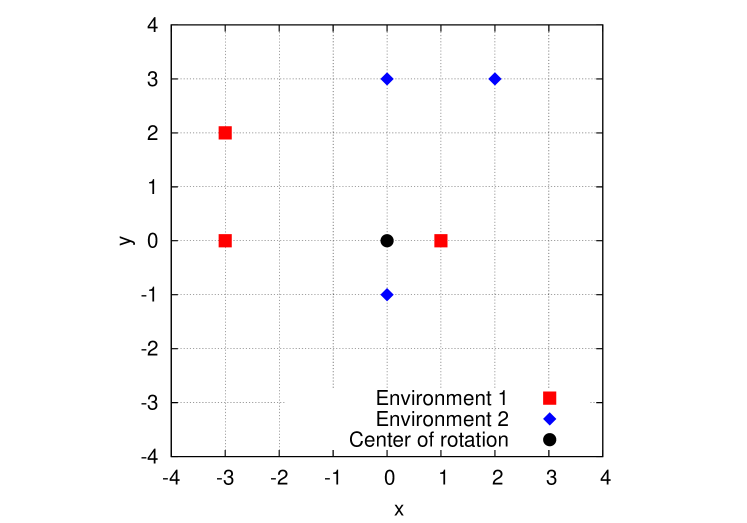
Figure 1: Example of two environments $C_{1}$ and $C_{2}$ representing the same configuration $\widetilde{C}$ in two dimensions.

II.2 Functional Representation of Atomic Configuration (Frac)

In this part we still consider systems with a single chemical element. Our goal is to represent a set of particles by a smooth probability density that can be manipulated more conveniently than a set of vectors. The idea is that a set of $n$ particles at positions $(q_{i})_{i=1}^{n}$ can be exactly represented by a set of Dirac functions $\delta_{q_{i}}$ at their positions:

$$\rho_{\{q_{1},\ldots,q_{n}\}}=\frac{1}{n}\sum_{i=1}^{n}\delta_{q_{i}}.$$ (4)

This expression is convenient since it is invariant with respect to permutation of atoms: we exploit this property in Section III. But this representation is unusable in practice, because the spectral expansion of a Dirac delta function is too slowly convergent. Approximating the Dirac delta function requires basis sets of very large dimension. It is more convenient to smooth out (4) and represent an environment by a density $\rho_{\sigma}$, where $\sigma$ is a smoothness parameter, as in Refs. Bartok2013repr, ; bartokthesis, . This density $\rho_{\sigma}$ can be interpreted as a density of mass, or as a probability density of presence, the particles’ positions being considered as realizations of a random variable in $\mathbb{R}^{3}$. As a result, we need to define appropriate functions $\varphi$ to represent the presence of one atom at position $0$ (other locations are obtained by translations of such functions). These functions should verify the following properties:

• regularity, e.g. $\varphi$ is continuous by parts;

• $\varphi$ is bounded with unit mass, i.e. $0\leq\varphi\leq 1$ and $\int_{\mathbb{R}^{3}}\varphi=1$;

• $\varphi$ is positive and reaches its maximal value at $q=0$;

• $\varphi(q)\xrightarrow[q\to+\infty]{}0$.

Note that we could restrict ourselves to more regular functions, for example infinitely differentiable ones. Several choices can be made, as made precise in section III.3, but for the sake of clarity we consider in the sequel the Gaussian case. The choice Bartok2013repr

$$\varphi^{\sigma}(q)=(2\pi\sigma^{2})^{-\frac{3}{2}}\exp\left(-\frac{\|q\|^{2}}{2\sigma^{2}}\right)$$ (5)

verifies the required properties to represent the presence of an atom. A configuration $C=(q_{i})_{i=1}^{n}\in\mathcal{C}$ can then be represented by the density

$$\rho_{\sigma}(q)=\frac{1}{n}\sum_{i=1}^{n}\varphi_{q_{i}}^{\sigma}(q)=\frac{1}{n}\sum_{i=1}^{n}\varphi^{\sigma}(q-q_{i}).$$ (6)

As an example, the functional representation of an atomic environment of a fluid with such a function is shown in Figure 2. The asymptotic behavior of this density shows that the functional representation (6) is a smoothed representation of atomic positions. Indeed, the Gaussian function tends to a Dirac delta function when $\sigma$ tends to $0$. As a result

$$\rho_{\sigma}=\frac{1}{n}\sum_{i=1}^{n}\varphi_{q_{i}}^{\sigma}\ \xrightarrow[\sigma\to 0]{}\rho_{\{q_{1},\ldots,q_{n}\}}=\frac{1}{n}\sum_{i=1}^{n}\delta_{q_{i}},$$

in the sense of distributions. More details about this functional representation are provided in section III.3.

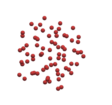
(a)

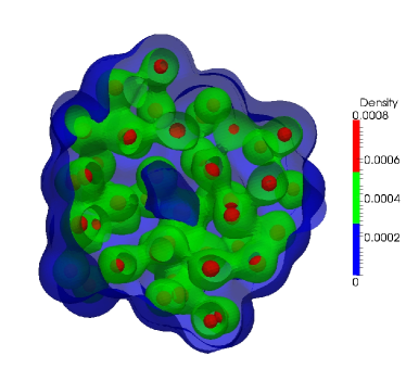
(b)

Figure 2: Example of atomic environment for a fluid with associated Frac

In some applications, it is convenient to consider only atoms within a cut-off radius of the origin. We introduce to this end a decreasing cut-off function $f_{\mathrm{cut}}:\mathbb{R}\mapsto\mathbb{R}$ such that

$$f_{\mathrm{cut}}(0)=1\,,\quad f_{\mathrm{cut}}(r)=0\ \mathrm{for}\ r\geq R_{\mathrm{cut}}.$$

For instance, Parrinello and Behler behler2007 ; behler2011atom ; behler2014ref choose

$$f_{\mathrm{cut}}(r)=\left\{\begin{array}[]{*2{>{\displaystyle}l}}\frac{1}{2}\left[\cos\left(\frac{\pi r}{R_{\mathrm{cut}}}\right)+1\right]\,,&r\leq R_{\mathrm{cut}},\\ 0\,,&r>R_{\mathrm{cut}}.\end{array}\right.$$ (7)

Of course other options may be considered, such as $f_{\mathrm{cut}}(r)=\mathds{1}_{\{r<R_{\mathrm{cut}}\}}(r)$. In this framework, an environment is now represented by its smoothed weighted density:

$$\rho_{R_{\mathrm{cut}}}(q)=\frac{\displaystyle\sum_{i=1}^{n}\varphi_{q_{i}}(q)f_{\mathrm{cut}}(\|q_{i}\|)}{\displaystyle\sum_{i=1}^{n}f_{\mathrm{cut}}(\|q_{i}\|)}.$$ (8)

The denominator in (8) is introduced in order for $\rho_{R_{\mathrm{cut}}}$ to be a probability density (i.e. with unit mass). From a physical viewpoint, it shows that we do not attach the same weight to each particle: atoms far away from the center have a smaller weight since they should contribute less to the description of the environment. It represents an effective number of particles in the neighborhood of the considered atom. All the following results are presented with the representation (6) but can be easily adapted with (8).

Let us emphasize some advantages of the Frac. First, it is invariant with respect to permutations of atoms of an environment. Secondly, it provides the same type of representation (a function on $\mathbb{R}^{3}$) whatever the number of atoms, which allows to compare configurations with different numbers of atoms. Finally, a distance between configurations can be naturally defined in this functional framework.

III Atomic Configuration Distance (Acd)

III.1 Single Element Systems

Once a Frac has been defined for systems with one chemical element, a natural way to derive a distance between configurations is to define a distance between their associated densities. A classical choice is the $L^{2}$ distance since it relies on a standard scalar product. Indeed, defining as in Ref. Bartok2013repr, the overlap integral

$$S(\rho_{1},\rho_{2})=\int_{\mathbb{R}^{3}}\rho_{1}\rho_{2},$$ (9)

the $L^{2}$ distance reads

$$\|\rho_{1}-\rho_{2}\|_{L^{2}}^{2}=S(\rho_{1},\rho_{1})-2S(\rho_{1},\rho_{2})+S(\rho_{2},\rho_{2}).$$ (10)

By identification between an environment and its density, we define the following distance, for $C_{1}=(q_{i})_{i=1}^{n_{1}}$, and $C_{2}=(q^{\prime}_{i})_{i=1}^{n_{2}}\in\mathcal{C}$:

$$\begin{array}[]{*2{>{\displaystyle}l}}d_{2}\left(C_{1},C_{2}\right)^{2}&=\frac{1}{n_{1}^{2}}\,\sum_{i,j=1}^{n_{1}}\int_{\mathbb{R}^{3}}\varphi_{q_{i}}(q)\varphi_{q_{j}}(q)\mbox{d}q\\ &-\,\frac{2}{n_{1}n_{2}}\,\sum_{i=1}^{n_{1}}\sum_{j=1}^{n_{2}}\int_{\mathbb{R}^{3}}\varphi_{q_{i}}(q)\varphi_{q^{\prime}_{j}}(q)\mbox{d}q\\ &+\,\frac{1}{n_{2}^{2}}\,\sum_{i,j=1}^{n_{2}}\int_{\mathbb{R}^{3}}\varphi_{q^{\prime}_{i}}(q)\varphi_{q^{\prime}_{j}}(q)\mbox{d}q.\end{array}$$ (11)

In order to construct a rotation invariant distance, we take the infimum over rotations of one representing environment, as done for the Rmsd coutsias2004 ; Theobald2005 . For two configurations $\widetilde{C}_{1}$, $\widetilde{C}_{2}\in\widetilde{\mathcal{C}}$, we choose two representing environments $C_{1}\in\widetilde{C}_{1}$ and $C_{2}\in\widetilde{C}_{2}$ belonging to each of these configurations and define:

$$\begin{array}[]{*2{>{\displaystyle}l}}\tilde{d_{2}}\left(\widetilde{C}_{1},\widetilde{C}_{2}\right)&=\underset{R\in\mathcal{R}}{\inf}\,d_{2}\,(C_{1},RC_{2})\\ &=\underset{R\in\mathcal{R}}{\inf}\,d_{2}\,(RC_{1},C_{2}),\end{array}$$ (12)

which is a distance on $\widetilde{\mathcal{C}}$ (see Appendix A). In practice, we compare one environment $C_{1}$ to another $C_{2}$ with (11) and estimate the rotation minimizing this quantity, as in a Rmsd framework Kabsch1976 . Nevertheless, there seems to be no simple expression of this optimal rotation, contrarily to the Rmsd case coutsias2004 ; Theobald2005 for which the optimal rotation is obtained as solution of a singular value decomposition. We describe a procedure to numerically estimate the optimal rotation in section III.2.

The Smooth Overlap of Atomic Positions (Soap) introduced in Ref. Bartok2013repr, also consists in taking a Gaussian function for $\varphi$ as in (5) but averaging over rotations by decomposing over spherical harmonics. Here, we also choose Gaussians, but rather consider the infimum over rotations. The idea is drawn from the Rmsd, and enables to define a permutation and rotation invariant distance on $\mathcal{C}$, or equivalently a distance on $\widetilde{\mathcal{C}}$. Moreover, in the Gaussian case, the overlap integral (9) has an analytical expression which alleviates the need for numerical quadrature. Indeed, the following formula holds (see Appendix B):

$$S(\rho_{1},\rho_{2})=\frac{\kappa^{-1}}{n_{1}n_{2}}\sum_{i=1}^{n_{1}}\sum_{j=1}^{n_{2}}\exp\left(-\frac{(q_{i}-q^{\prime}_{j})^{2}}{4\sigma^{2}}\right),$$ (13)

with $\kappa=8(\pi\sigma^{2})^{\frac{3}{2}}$. The permutation invariant measure of distance based on (11) then simplifies as

$$\begin{array}[]{*2{>{\displaystyle}l}}d_{2}\left(C_{1},C_{2}\right)^{2}&=\frac{\kappa^{-1}}{n_{1}^{2}}\,\sum_{i,j=1}^{n_{1}}\exp\left(-\frac{(q_{i}-q_{j})^{2}}{4\sigma^{2}}\right)\\ &-\,\frac{2\kappa^{-1}}{n_{1}n_{2}}\,\sum_{i=1}^{n_{1}}\sum_{j=1}^{n_{2}}\exp\left(-\frac{(q_{i}-q_{j}^{\prime})^{2}}{4\sigma^{2}}\right)\\ &+\,\frac{\kappa^{-1}}{n_{2}^{2}}\,\sum_{i,j=1}^{n_{2}}\exp\left(-\frac{(q_{i}^{\prime}-q_{j}^{\prime})^{2}}{4\sigma^{2}}\right).\end{array}$$ (14)

A permutation and rotation invariant distance is finally obtained with (12). This is the formula we use in the applications presented in this work, with the cut-off function as given in Section II.2. Moreover, asymptotic results when $\sigma\to 0$ and $\sigma\to+\infty$ are studied in Appendix C.

Finally, as noticed in Ref. Bartok2013repr, , the quantity

$$S(C_{1},C_{2})=\frac{1}{n_{1}n_{2}}\sum_{i=1}^{n_{1}}\sum_{j=1}^{n_{2}}\exp\left(-\frac{(q_{i}-q^{\prime}_{j})^{2}}{4\sigma^{2}}\right)$$

is a permutation invariant measure of similarity between atomic environments. Setting

$$\tilde{S}(C_{1},C_{2})=\frac{\underset{R\in\mathcal{R}}{\sup}S(C_{1},RC_{2})}{\sqrt{S(C_{1},C_{1})S(C_{2},C_{2})}},$$

we define a kernel on the space of configurations $\widetilde{\mathcal{C}}$ that can be directly used for Machine Learning approaches, as SoapBartok2013repr . The supremum ensures that the optimal rotation maximizes the similarity of the structures.

III.2 Optimal Rotation

From a practical viewpoint, we search the minimum in (12) by parameterizing a rotation $R$ in terms of the Euler anglesrose1995elementary ; varshalovich1988quantum $(\alpha,\beta,\gamma)$ , but other choices could be made, such as quaternions coutsias2004 ; Theobald2005 . The three angles correspond to three rotations around different axes. We use rotations of angle $\nu$ over axes $x$ and $z$, defined by the following rotation matrices:

$$R_{x}(\nu)=\begin{pmatrix}1&0&0\\ 0&\cos(\nu)&-\sin(\nu)\\ 0&\sin(\nu)&\cos(\nu)\end{pmatrix}\,,$$

$$R_{z}(\nu)=\begin{pmatrix}\cos(\nu)&-\sin(\nu)&0\\ \sin(\nu)&\cos(\nu)&0\\ 0&0&1\end{pmatrix}.$$

A rigid body rotation rose1995elementary ; varshalovich1988quantum is then defined by $R_{\alpha,\beta,\gamma}=R_{z}(\gamma)R_{x}(\beta)R_{z}(\alpha)$ with $(\alpha,\beta,\gamma)\in[0,2\pi]\times[0,\pi]\times[0,2\pi]$. Therefore, the optimization is performed in this 3-dimensional compact space. We use a Monte Carlo procedure (simulated annealing SA1987 ; SA2005 , see Appendix D) to search for the minimum.

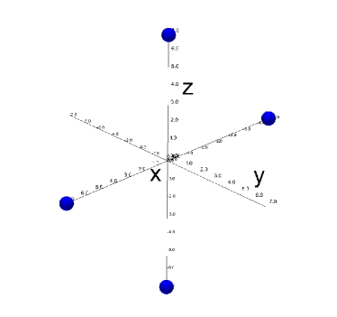
(a)

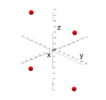
(b)

Figure 3: Example of two environments $C_{1}$ and $C_{2}$ representing the same configuration $\widetilde{C}$ in three dimensions.

In order to test the method, we fix two environments $C_{1}$, $C_{2}$ with 4 particles in each one and $C_{1}=\sigma RC_{2}$ for some rotation $R$ and permutation $\sigma$ (see Figure 3), so that $C_{1}$ and $C_{2}$ represent the same configuration. Then we study the mapping $J:(\alpha,\beta,\gamma)\mapsto d_{2}(C_{1},R_{\alpha,\beta,\gamma}C_{2})$. In Figure 4, we display isosurfaces of $J$. We see that the minimum of this function is indeed 0, and that several rotations meet this minimum (given that the system has several symmetries). Moreover, a realization of simulated annealing is plotted, showing that the global minimum is found by a numerical method. As a second example, two environments $C_{1}$, $C_{2}$ of a Lennard-Jones fluid (see Appendix F) are considered. An example of such an environment is represented in Figure 2 (a). In Figure 5, we plot isosurfaces of $J$ with a realization of simulated annealing for these environments. Here, two local minima are found, but only one is the global minimum.

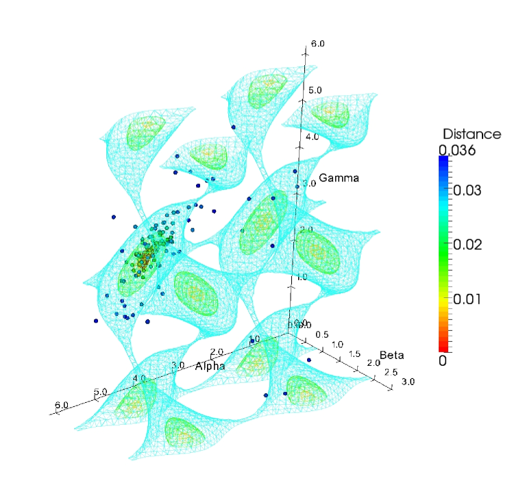
Figure 4: Isovalues of the mapping $J:(\alpha,\beta,\gamma)\mapsto d_{2}(C_{1},R_{\alpha,\beta,\gamma}C_{2})$ when $C_{1}$ and $C_{2}$ belong to the same class. The points represent the iterates of a simulated annealing procedure.

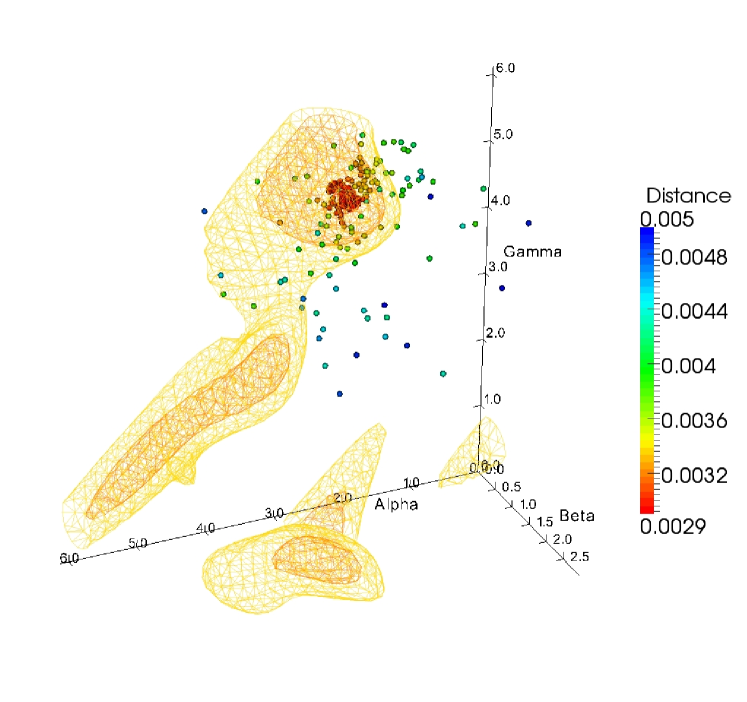
Figure 5: A realistic example, two configurations of a fluid. The wire frame represents level sets of the mapping $J:(\alpha,\beta,\gamma)\mapsto d_{2}(C_{1},R_{\alpha,\beta,\gamma}C_{2})$ and the points a simulated annealing procedure.

We studied more specifically the case of the Gaussian Frac with $L^{2}$ distance, since the analytical formula (14) allows to dramatically reduce the computational cost of its evaluation. In this case, the parameter $\sigma$, if not essential from a theoretical viewpoint, plays a role in numerical applications. Indeed, changing $\sigma$ does not change the position of the global minimum, but affects the gradient of function $J$. A large value of $\sigma$ leads to a shallow function, whereas a small $\sigma$ leads to a peaked function $J$. Therefore, the numerical efficiency of the optimization procedure depends on the value of this parameter.

III.3 Generalizations

We considered in the previous section the particular case of Gaussian functions $\varphi$ for representing atoms. Let us however emphasize that other choices are possible and in fact many other generalizations of Frac can be proposed.

First, several choices are available for representing the presence of one atom, for example in dimension $1$:

• $\displaystyle\varphi_{1}(q)=(2\pi\sigma^{2})^{-\frac{1}{2}}\exp\left(-\frac{\|q\|^{2}}{2\sigma^{2}}\right)$

• $\displaystyle\varphi_{2}(q)=\frac{c}{\sigma}\exp\left(-\frac{1}{\sigma^{2}-\|q\|^{2}}\right)$

• $\displaystyle\varphi_{3}(q)=\frac{1}{2\sigma}\mathds{1}_{\{\|q\|\leq\sigma\}}(q)$

• $\displaystyle\varphi_{4}(q)=\left\{\begin{array}[]{*2{>{\displaystyle}l}}q+\sigma,&\mbox{for }q\in(-\sigma,0),\\ -q+\sigma,&\mbox{for }q\in(0,\sigma),\\ 0,&\mathrm{otherwise}.\end{array}\right.$

The idea always is to put weight in the vicinity of the central atom, with more or less smoothness and accuracy. More formally, this reduces to using an approximation of a Dirac function in the sense of distributions. The indicator function in dimension 3, $\varphi^{\sigma}(q)=(\frac{4}{3}\pi\sigma^{3})^{-1}\mathds{1}_{\{\|q\|<\sigma\}}(q)$, represents the atom as a volume in space. Other functions represent a mass density vanishing more or less smoothly. Another interpretation is probabilistic. We can consider that the positions of neighbors are realizations of a random variable drawn according to a density $\chi$. In this case, the density (6) with the choice $\varphi^{\sigma}(q)=(\frac{4}{3}\pi\sigma^{3})^{-1}\mathds{1}_{\{\|q\|<\sigma\}}(q)$ corresponds to a histogram in $\mathbb{R}^{3}$ approximating this measure $\chi$. The Gaussian choice corresponds to the Gauss kernel approximation of $\chi$, which is a particular case of non-parametric estimation of a probability density silverman1986density ; hardle2004nonparametric , and can be interpreted as a smoothed histogram.

From a formal point of view, the measure $\rho_{\sigma}$ defined in (6) corresponds to the convolution of the measure $\rho_{\{q_{1},\ldots,q_{n}\}}$ defined in (4) with the shape function $\varphi^{\sigma}$, which reads:

$$\begin{array}[]{*2{>{\displaystyle}l}}\rho_{\sigma}(q)&=\rho_{\{q_{1},\ldots,q_{n}\}}\star\varphi^{\sigma}(q)\\ &=\int_{\mathbb{R}^{3}}\rho_{\{q_{1},\ldots,q_{n}\}}(q^{\prime})\varphi^{\sigma}(q-q^{\prime})\mbox{d}q^{\prime}.\end{array}$$

As a result, the function $\varphi^{\sigma}$ can be interpreted either as a way to represent an atom or as a shape function in a regularizing convolution of the measure $\rho_{\{q_{1},\ldots,q_{n}\}}$.

Another possible extension of the method is to consider different distances between densities, such as $L^{p}(w)$ distances where $p\in\mathbb{N}^{*}$ and $w$ is typically a rotation invariant non-negative weight function with unit mass. In this case,

$$\|\rho_{1}-\rho_{2}\|_{L^{p}(w)}=\left(\int_{\mathbb{R}^{3}}|\rho_{1}-\rho_{2}|^{p}w\right)^{\frac{1}{p}}.$$ (15)

The weight $w$ can be used for example to give a higher importance to some region of space. In our case, the choice $p=2$ is reasonable not only because it is coherent with the distances generally used (for example between sets of vectors for the Rmsd), but also because it relies on a scalar product that proves to be convenient for calculations. On the other hand, no analytical expressions are in general available for the extensions listed so far. They are, as a result, more computationally expensive in practice.

It is nonetheless possible to consider another way to generalize Acd, by directly starting from (13) and replacing the Gaussian function by any shape function $\varphi^{\sigma}$ verifying the properties outlined in Section II.2 (typically one presented at the begining of this section). This amounts to considering

$$S(C_{1},C_{2})=\frac{1}{n_{1}n_{2}}\sum_{i=1}^{n_{1}}\sum_{j=1}^{n_{2}}\varphi^{\sigma}(\|q_{i}-q^{\prime}_{j}\|).$$

The function $\varphi^{\sigma}$ now plays the role of a correlation between two particles. If the particles are close with respect to the bandwidth $\sigma$, their distance is small and $\varphi^{\sigma}$ is typically close to 1. If they are distant, $\varphi^{\sigma}$ is close to 0. This opens a wide range of perspectives for constructing distances for which the same conclusions as in Section III can be drawn.

III.4 Multi-elements Systems

We now extend the previous results to systems of $p$ chemical elements, which offer a wider range of applications. In our framework, a natural way to represent an environment of $p$ chemical species is to represent it as a product of environments of individual species:

$$\mathcal{C}^{p}=\underbrace{\mathcal{C}\times\ldots\times\mathcal{C}}_{p\,\mathrm{times}}.$$ (16)

The only issue is to correctly describe admissible rotations and permutations of such a system. For a multi-element environment $C=(C^{1},C^{2},\ldots,C^{p})\in\mathcal{C}^{p}$, with $n_{i}$ elements for each $C^{i}$, we define a permutation of the system $\sigma=(\sigma_{1},\sigma_{2},\ldots,\sigma_{p})\in\mathcal{S}_{n}=\mathcal{S}_{n_{1}}\times\ldots\times\mathcal{S}_{n_{p}}$, as

$$\sigma C=\left(\sigma_{1}C^{1},\sigma_{2}C^{2},\ldots,\sigma_{p}C^{p}\right),$$

and a rotation $R\in\mathcal{R}$ as

$$RC=\left(RC^{1},RC^{2},\ldots,RC^{p}\right).$$

First, this means that permutations are allowed only between elements of the same chemical element (and not with other species). Secondly, rotations are defined on the whole system, so they modify each environment in the same way. It is then straightforward to define the equivalence relationship $\sim$ as in Section II.1. For $C_{1}=((q_{i}^{1})_{i=1}^{n_{1}},\ldots,(q_{i}^{p})_{i=1}^{n_{p}})\in\mathcal{C}^{p}$, $C_{2}=((q_{i}^{\prime 1})_{i=1}^{m_{1}},\ldots,(q_{i}^{\prime p})_{i=1}^{m_{p}})\in\mathcal{C}^{p}$,

$$C_{1}\sim C_{2}\Leftrightarrow\left|\begin{aligned} &\forall\,i\leq p,\,n_{i}=m_{i}\mbox{ and }\exists\,\sigma\in\mathcal{S}_{n},\,\exists\,R\in\mathcal{R}\\ &\quad\mbox{such that }\,C_{1}=\sigma RC_{2}.\end{aligned}\right.$$

We next define $\widetilde{\mathcal{C}}^{p}=\mathcal{C}^{p}_{\,/\sim}$. In other words, two environments belong to the same class if and only if one can be written as a rotation of the other up to a permutation of atoms in each species. Now, we can introduce a distance between two multi-elements environments as the sum of distances for each single element, that is:

$$d_{2}^{p}(C_{1},C_{2})^{2}=d_{2}(C_{1}^{1},C_{2}^{1})^{2}+\ldots+d_{2}(C_{1}^{p},C_{2}^{p})^{2},$$

where $d_{2}$ is defined (14) in the Gaussian case. This measure of distance is permutation invariant thanks to the Frac framework. Now, to make this distance rotation invariant, we again minimize over rotations. For two configurations $\widetilde{C}_{1}$, $\widetilde{C}_{2}\in\widetilde{\mathcal{C}}^{p}$, represented by two environments $C_{1}\in\widetilde{C}_{1}$ and $C_{2}\in\widetilde{C}_{2}$, we set

$$\tilde{d}^{p}\left(\widetilde{C}_{1},\widetilde{C}_{2}\right)=\underset{R\in\mathcal{R}}{\inf}\,\sqrt{\,\sum_{i=1}^{p}\,d_{2}(C_{1}^{i},RC_{2}^{i})^{2}}.$$ (17)

Note that since rotations act in the same way on all single environment (i.e. for each chemical element), the minimum is taken over the sum of distances with the same rotation for each species. If one wants to give various importance to the different elements, a family of distances may be introduced with a vector of positive weights $w\in(\mathbb{R}_{+})^{p}$ with $\sum_{i=1}^{p}w_{i}=1$, by setting

$$\tilde{d}_{w}^{p}\left(\widetilde{C}_{1},\widetilde{C}_{2}\right)=\underset{R\in\mathcal{R}}{\inf}\,\sqrt{\,\sum_{i=1}^{p}\,w_{i}\,d_{2}(C_{1}^{i},RC_{2}^{i})^{2}}.$$

We can check that $\tilde{d}_{w}^{p}$ verifies all the properties of a distance on $\widetilde{\mathcal{C}}^{p}$ as in the single element case. Of course, an extension to configurations in a cut-off radius $\mathcal{C}_{\mathrm{cut}}$ is straightforward following the discussion of Section II.2.

IV Applications

IV.1 Faithfulness of fingerprints

Fingerprints appear in several areas of chemical physics, for example for representing Potential Energy Surfaces (PES) with Machines Learning approaches Bartok2013repr ; bartokthesis ; behler2007 ; behler2011atom ; behler2014ref or local structure recognition schutt2014 ; SadeghiMetric2013 ; Bartok2013repr ; bartokthesis . The problem with these methods is that two environments that differ by a rotation or a permutation are understood as different inputs for the model, and may lead to different outputs, whereas the energy and the forces remain unchanged. Moreover, the dimension of the input vector has to be constant, and should not depend on the number of neighbors. Therefore, fingerprints (or descriptors) generally consist of functions of neighboring atoms, invariant by rotation and permutation. They are supposed to characterize the structure of an atomic environment. Formally, they can be defined as a mapping $\Phi:\mathcal{C}\mapsto\mathbb{R}^{m}$ such that for any permutation $\sigma\in\mathcal{S}$ and rotation $R\in\mathcal{R}$, it holds $\Phi(\sigma RC)=\Phi(C)$. We already mentioned in the introduction some appropriate descriptors for such applications, especially the ones based on eigenvalues of matrices SadeghiMetric2013 ; Bartok2013repr ; schutt2014 ; Rupp2012 , bond-order parameters and bi-spectrum Bartok2013repr ; bartokthesis and symmetry functions behler2007 ; behler2011atom ; behler2014ref .

As an example, we chose to study the faithfulness of representation of two types of symmetry functions behler2007 ; behler2011atom ; behler2014ref , but all the cited descriptors could be tested. We investigate the relevance of two-body functions $G^{2}$ and three-body functions $G^{3}$ (see (18) and (19) below). The sums run over the neighboring atoms and $\theta_{jk}$ is the angle associated with the triplet made of the central particle and its neighbors $j,k$. Moreover, $f_{\mathrm{cut}}$ is chosen as in (7) and $R_{s}$, $\eta$, $\lambda$ and $\zeta$ are real parameters.

$$G^{2}=\sum_{i=1}^{n}\mathrm{e}^{-\eta(\|q_{i}\|-R_{s})^{2}}f_{\mathrm{cut}}(\|q_{i}\|).$$ (18)

$$G^{3}=2^{1-\zeta}\sum_{j,k=1}^{n}(1+\lambda\cos(\theta_{jk}))^{\zeta}\mathrm{e}^{-\eta\left(\|q_{j}\|^{2}+\|q_{k}\|^{2}+\|q_{j}-q_{k}\|^{2}\right)}f_{\mathrm{cut}}(\|q_{j}\|)f_{\mathrm{cut}}(\|q_{k}\|)f_{\mathrm{cut}}(\|q_{j}-q_{k}\|).$$ (19)

The coordinates of $\Phi$ in $\mathbb{R}^{m}$ are then obtained by calculating the functions $G^{2}$ and $G^{3}$ for various values of the parameters $\eta$, $R_{s}$, $\lambda$, $\zeta$. One can easily check that $\Phi$ is invariant under rotation and permutation. Our goal is to study the relevance of this choice of fingerprint $\Phi$: Is this representation able to discriminate different structures ? What are the optimal parameters? How many functions should be used?

Our strategy is to estimate for various couples of configurations $C_{i}$, $C_{j}$ the distance in the space of descriptors $\|\Phi(C_{i})-\Phi(C_{j})\|$, and the distance in the Cartesian space $\tilde{d}_{2}(C_{i},C_{j})$, before computing their correlation. We will then be able to understand whether the representation is ambiguous or not: typically, a wrong representation would lead to high Atomic Configuration Distance $\tilde{d}_{2}$ (Acd) and low fingerprint difference, or conversely low Acd and high fingerprint distance.

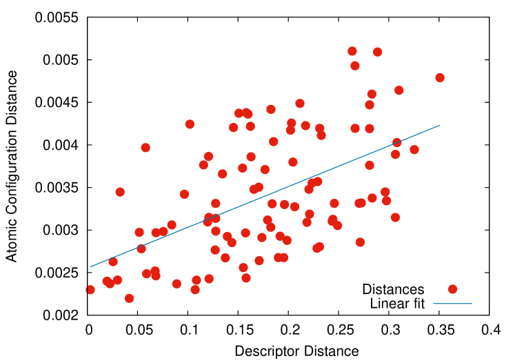
Figure 6: Correlation between Acd and descriptor distance for two fingerprints, $\sigma=2$

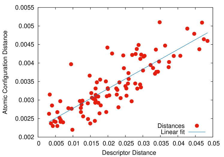
Figure 7: Correlation between Acd and descriptor distance for a new set of fingerprints, $\sigma=2$

We generate a set of configurations $C_{i}$ of a Lennard-Jones fluid with a molecular dynamics simulation (see Appendix F). As a first example, we apply the procedure by taking only one $G^{2}$ and one $G^{3}$ functions to represent the environment, with $R_{\mathrm{cut}}=8.52$ Å, $\eta=0.5$, $R_{s}=0$ Å, $\lambda=-1$ and $\zeta=1$. In Figure 6, we observe the expected correlation between the descriptor distance and the Acd for this choice of descriptors but with an important dispersion. After a manual trial and error search, we found a set of functions giving a better correlation (see Appendix E), as displayed in Figure 7. To quantify the increase of faithfulness of the fingerprints, and given that the correlation seems linear, we perform the least square fit of the Acd as a function of the descriptor distance, and compute for each case the associated correlation coefficient $r\in[0,1]$. The first set of fingerprints has a correlation $r=0.55$ and the second $r=0.84$.

Another point is to estimate the necessary and sufficient number of functions to describe the configurations. Figure 8 shows the evolution of the correlation coefficients $r$ when adding $G^{2}$ functions. We fix $R_{\mathrm{cut}}=8.52$ Å, $R_{s}=0$ Å, and consider additional values of $\eta$ obtained as $\eta_{1}=1$, $\eta_{2}=\frac{\eta_{1}}{2}$, $\eta_{3}=\frac{\eta_{2}}{2}$, …until $\eta_{13}=\frac{\eta_{12}}{2}$.. Then we choose the same values of $\eta$ for $R_{s}=2.$ Å. This makes a total of 26 functions. We add the descriptors one by one, perform the least square fit for each corresponding fingerprint and study the evolution of the correlation coefficient $r$. We first observe an increasing correlation as expected, but after a critical number of functions, $r$ decreases or remains stable. We also note an increase of the correlation when adding the first symmetry functions with $R_{s}=2$ Å. Other functions should be added, such as $G^{3}$ functions, to increase the representation capacity of the set of descriptors. The decrease of correlation may seem surprising at first. It is due to the fact that lower values of $\eta$ tend to generate functions describing the environment far from the central particle. On the other hand, the Acd has been implemented with a cut-off function as described in section II.2. As a result, the description of the environment near the cut-off radius $R_{\mathrm{cut}}$ is less correlated to the Acd, hence the decreased correlation. This point is important in practice for several applications. Typically for numerical potentials, using symmetry functions describing the environment near the cut-off radius is not relevant since nearer neighbors have a stronger influence on the potential.

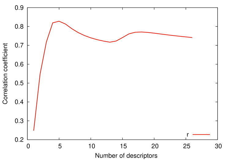
Figure 8: Evolution of the correlation coefficient $r$ when adding $G^{2}$ functions

Let us now discuss how this procedure can be used to optimize the set of parameters used for the descriptors. As a simple application, we aim at optimizing the parameter $\eta$ in (18) for only one $G^{2}$ function. We fix $R_{s}=0$ Å, $R_{\mathrm{cut}}=8.52$ Åand study the correlation coefficient $r$ as a function of $\eta$ in Figure 9. The graph shows a maximal value around $\eta^{*}=0.0381$, which corresponds to a Gaussian of standard deviation $3.6$. It can be understood as a typical length to describe the system around its central atom. The correlation for low values of $\sigma$ is still correct, but it drastically decreases when $\eta$ becomes too large. This can be explained by the fact that the variance of the Gaussian tends to zero when $\eta$ becomes large, so the $G^{2}$ function takes values close to $0$ whatever the environment, and does not describe the environment anymore. The correlation graph associated with the optimal value $\eta^{*}$ is displayed in Figure 10. Even though the correlation is good, we observe as in Figure 6 that for some couples of configurations, the descriptor distance is $0$ whereas the Acd is not, which is a crucial problem. It suggests that our descriptor should also maximize the quantity

$$\underset{i,j}{\min}\ \|\Phi(C_{i})-\Phi(C_{j})\|.$$

Several tracks can therefore be followed when $C_{i}$ and $C_{j}$ do not belong to the same configuration to optimize a fingerprint. First, a criterium to optimize should be chosen (maximizing the correlation or minimizing the lack of injectivity of $\Phi$). As a second step, the set of symmetry functions can be optimized either by a greedy technique (adding the functions one by one with associated optimized parameters) or by defining a set of functions and optimizing all parameters together. The first option does not provide the optimal set of functions, but is easier to implement. The second one possibly requires to explore a large set of parameters, and more advanced optimization methods should be investigated.

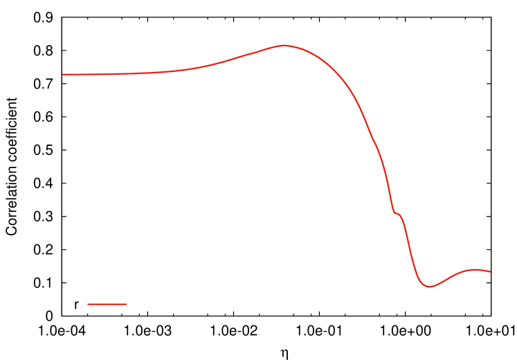
Figure 9: Evolution of correlation coefficient $r$ with $\eta$

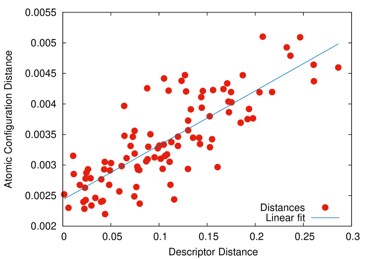
Figure 10: Correlation between Acd and descriptor distance for one optimized $G^{2}$ function

To summarize, the Acd is a way to quantify the conservation of information when using a descriptor. It can be used to indicate if functions are relevant to represent a given set of structures. It also allows to quantify the improvement in the representation obtained by adding a new describing function, and to optimize the parameters in the descriptors. This is particularly important in the context of Machine Learning, since the dimension of the fingerprint $m$ (i.e. the number of functions in the representation) is the dimension of the interpolation space for the methods (Neural Networks or Kernel methods). Reducing the size of the input space $\mathbb{R}^{m}$ is of crucial importance to increase the efficiency of this interpolation (or learning) procedure. Lower values of $m$ also allow to decrease the computational cost of evaluating the numerical potential, which is significant in order to perform faster Molecular Dynamics simulations.

IV.2 Structural Analysis

The goal of this section is to demonstrate in a simple case that our method can be used to identify the local structure of a material. We restrict ourselves to the structural analysis of a crystal with one chemical element, but extensions to crystals with several elements or even molecules are straightforward. For the testing procedure, we gather a database of crystalline structures $C_{i}$ at $0$ Kelvin (at a given density, see Appendix F for more details on the generation of this database):

• Body Centered Cubic (BCC),

• Face Centered Cubic (FCC),

• Simple Cubic (CS),

• Hexagonal Close Packed (HCP)

• diamond,

• liquid,

• Sn$\beta$ ($\beta$ structure of tin).

We next compare a structure $C$ of FCC at 100 Kelvins obtained by molecular dynamics simulation to each element of the database $C_{i}$, by computing the distance in the fingerprints space $\|\Phi(C)-\Phi(C_{i})\|$ and Acd $\tilde{d}_{2}(C,C_{i})$. We use the fingerprint described in Appendix E. Figure 11 represents $\tilde{d}^{2}(C,C_{i})$ as a function of $\|\Phi(C)-\Phi(C_{i})\|$ for each reference structure $C_{i}$. For both Acd and fingerprints, the structure at 100 Kelvin is closer to FCC than to any other structure. This shows that Acd is efficient in recognizing the local structure of a material, and it also validates the choice of fingerprint used for the recognition of these environments. In order to better understand the influence of the smearing parameter $\sigma$, we display in Figure 12 the evolution of the Atomic Configuration Distance as a function of $\sigma$. The numerical values vary but the conclusion remains unchanged: the distance to the FCC structure is always the lowest. When $\sigma$ decreases, the accuracy of the distance increases, so small variations of the structure due to thermal fluctuations tend to be understood as a structural difference. On the other hand, when $\sigma$ is large, the precision is very low (or equivalently, the representing densities are very smooth), and all the configurations tend to be recognized as equivalent. The asymptotic behavior when $\sigma$ tends to 0 is also displayed; the distance scales as $\sigma^{-\nicefrac{{3}}{{2}}}$, as predicted by the analysis performed in Appendix C. The same behavior is observed for larger values of $\sigma$. Lastly, this distance induces a classification of similarity between structures. Indeed, Figure 13 shows the distance to each reference structure over the distance to FCC. All distances are larger than the distance to FCC, but with an ordering. Indeed, the distance to HCP and BCC is higher than the distance to FCC typically by a factor 1.5 or 2. On the other hand, distances to the other elements up to 4 times higher than the distance to FCC. This can be explained by the chemical similarity of HCP and BCC with the FCC structure. The chosen descriptor fails to provide this detailed study, since its distance to HCP is the highest one.

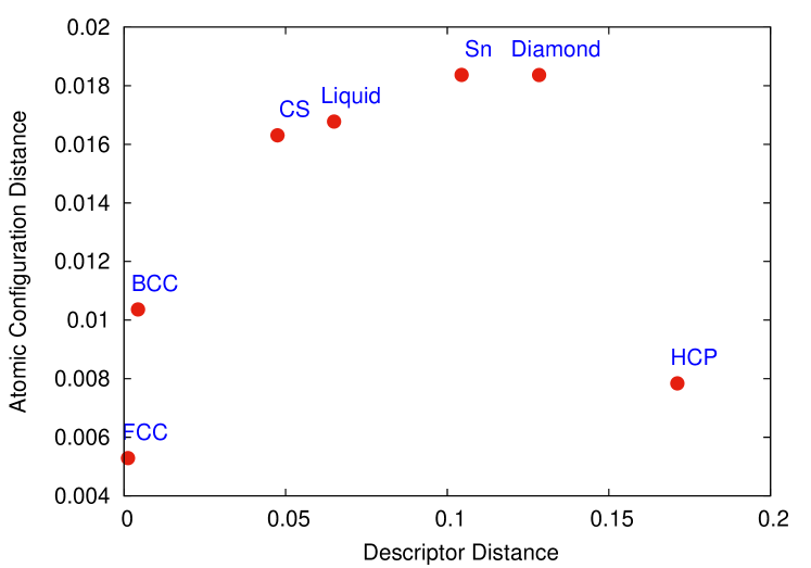
Figure 11: Distance from structure $C$ to reference structures, $\sigma=1$

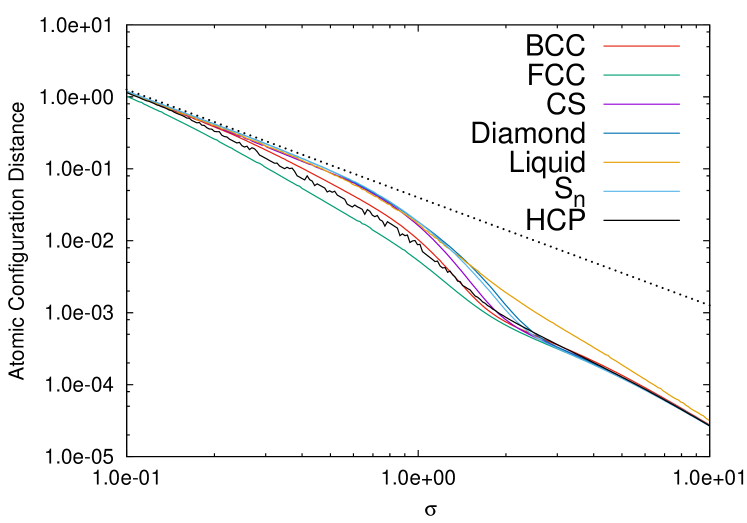
Figure 12: Atomic Configuration Distance to each reference structure as a function of $\sigma$

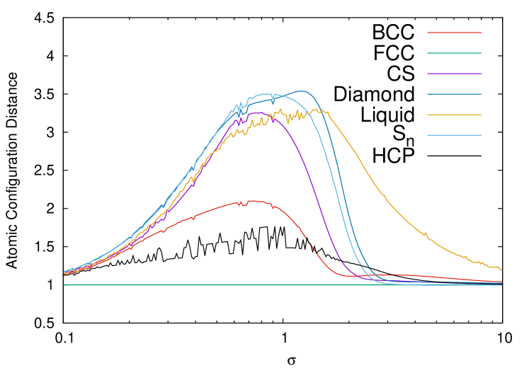
Figure 13: Atomic Configuration Distance to each reference structure normalized by the distance to FCC, as a function of $\sigma$

V Conclusion

Our goal in this work was to compare atomic configurations for various purposes, such as structure recognition or Machine Learning methods. To this end, we introduced a formal description of what we call atomic environment and atomic configuration, which provides a firm mathematical ground for defining a distance between configurations. Then, we showed that an environment can be represented as a permutation invariant density of probability, the Frac. This consideration naturally led us to define a permutation invariant distance between atomic environments of an arbitrary number of atoms $n_{1}$ and $n_{2}$. In particular, the Gaussian case provides an analytical distance whose computational cost scales as $n_{1}n_{2}$. We showed that taking the minimum over rotations of this distance creates a permutation and rotation invariant Atomic Configuration Distance (Acd). This means that a distance can be defined between two configurations. The significant difference with previous methodologies (notably Rmsd) is that the Acd is intrinsically permutation invariant, so that performing the minimum over permutations is unnecessary, and comparisons of environments with hundreds of atoms become tractable. This is of paramount importance for condensed matter systems.

Many applications can be envisioned. We considered two of them as an example. First, we studied the capability of fingerprints to reproduce the configurational information of a structure. This is of critical importance in several fields, in particular Machine Learning methods for numerical potentials. We showed that the introduced distance does not answer the issue of the choice of the descriptors by itself, but it provides a quantitative assessment of the improvement in the description provided by an additional representing function. This allows typically to implement greedy techniques, where parameters of a new function are optimized in order to obtain the maximal correlation $r$ between the Acd and the descriptor’s distance. A second application is structural analysis. By comparing a local structure to a reference data set of structures at 0 Kelvin, we showed that the Acd (12) is able to recognize the structure of a material at a positive temperature. Let us however mention that our methodology is not a way to characterize a structure from scratch. If the studied structure is not in the database, it will not be recognized.

Finally, we want to emphasize that we described the presented tools in a quite general and abstract way to allow for various applications. At several points of the derivation of the distances, choices can be made (such as the functions for representing the presence of an atom in the Frac or the norm to compare densities). Moreover, other applications can be considered: comparing molecules, testing other fingerprints, or using directly the similarity $S$ defined in (13) as a Kernel, as for the SoapBartok2013repr , (but taking the minimum over rotations rather than integrating over them and using the analytical expression (13)). Another important issue is the sparsification, i.e. the construction of a database minimizing the redundancy of information. Indeed, in the context of numerical potentials, it is crucial to have the smallest possible database to decrease the computation cost of the potential.

Appendix A Proof that ACD is a Distance

We here prove that the application defined in (12) is a distance on $\widetilde{\mathcal{C}}$. We remind that to be a distance on $\widetilde{\mathcal{C}}$, $\tilde{d_{2}}$ must verify, for any configurations $\widetilde{C}_{1}$, $\widetilde{C}_{2}$, $\widetilde{C}$$\in\widetilde{\mathcal{C}}$, the following properties:

• $\tilde{d_{2}}(\widetilde{C}_{1},\widetilde{C}_{2})=\tilde{d_{2}}(\widetilde{C}_{2},\widetilde{C}_{1})$,

• $\tilde{d_{2}}(\widetilde{C}_{1},\widetilde{C}_{2})=0$ if and only if $\widetilde{C}_{1}=\widetilde{C}_{2}$,

• $\tilde{d_{2}}(\widetilde{C}_{1},\widetilde{C}_{2})\leq\tilde{d_{2}}(\widetilde{C}_{1},\widetilde{C})+\tilde{d_{2}}(\widetilde{C},\widetilde{C}_{2})$.

First, $d_{2}$ being invariant by permutation, and since the rotation can be taken over $C_{1}$ or $C_{2}$ in (12), the definition of the distance is easily seen to be independent of the choice of the representing environments $C_{1}\in\widetilde{C}_{1}$ and $C_{2}\in\widetilde{C}_{2}$. Secondly, the optimization problem always has a solution since the space of rotations $\mathcal{R}$ is compact and the application $R\mapsto d_{2}\,(C_{1},RC_{2})$ is continuous. Therefore, the application is well-defined on $\widetilde{\mathcal{C}}\times\widetilde{\mathcal{C}}$. Now, the triangle inequality results from the isomorphism with the associated densities $\rho_{1}$, $\rho_{2}$. More precisely, for another configuration $\widetilde{C}\in\widetilde{\mathcal{C}}$, with a representing element $C\in\widetilde{C}$ and associated density $\rho$,

$$\|\rho_{1}-\rho_{2}\|_{L^{2}}\leq\|\rho_{1}-\rho\|_{L^{2}}+\|\rho-\rho_{2}\|_{L^{2}},$$

So, for any rotation $R$,

$$d_{2}(C_{1},RC_{2})\leq d_{2}(C_{1},C)+d_{2}(C,RC_{2}).$$

Moreover, given that $C\in\widetilde{C}$ is arbitrary, we can choose it such that $d_{2}(C_{1},C)=\underset{C^{\prime}\in\widetilde{C}}{\inf}d_{2}(C_{1},C^{\prime})$, which leads to

$$d_{2}(C_{1},RC_{2})\leq\tilde{d_{2}}(\widetilde{C}_{1},\widetilde{C})+d_{2}(C,RC_{2}).$$

Now, by taking the infimum over rotations $R$, first on the left hand side, and then on the right side, we obtain the triangle inequality

$$\tilde{d_{2}}(\widetilde{C}_{1},\widetilde{C}_{2})\leq\tilde{d_{2}}(\widetilde{C}_{1},\widetilde{C})+\tilde{d_{2}}(\widetilde{C},\widetilde{C}_{2}).$$

The last point is to prove that $\widetilde{C}_{1}=\widetilde{C}_{2}$ if and only if $\tilde{d_{2}}(\widetilde{C}_{1},\widetilde{C}_{2})=0$. First, it is clear that $\tilde{d_{2}}(\widetilde{C},\widetilde{C})=0$ for any $\widetilde{C}\in\widetilde{\mathcal{C}}$. Now, take $\widetilde{C}_{1}$, $\widetilde{C}_{2}\in\widetilde{\mathcal{C}}$ and $C_{1}\in\widetilde{C}_{1}$, $C_{2}\in\widetilde{C}_{2}$ such that $\tilde{d_{2}}(\widetilde{C}_{1},\widetilde{C}_{2})=0$. This implies

$$\underset{R\in\mathcal{R}}{\inf}\,d_{2}\,(C_{1},RC_{2})=0.$$

Therefore, there exists $R_{0}\in\mathcal{R}$ such that $d_{2}\,(C_{1},R_{0}C_{2})=0$, and given that $d_{2}$ is a distance up to a permutation, there exists $\sigma_{0}\in\mathcal{S}$ such that $C_{1}=\sigma_{0}R_{0}C_{2}$, i.e. $C_{1}$ and $C_{2}$ belong to the same class and $\widetilde{C}_{1}=\widetilde{C}_{2}$.

Appendix B Analytical Computation of the overlap matrices in the Gaussian case

We prove formulas (13) and (14). First,

$$S(\rho_{1},\rho_{2})=\int_{\mathbb{R}^{3}}\rho_{1}\rho_{2}=\frac{1}{n_{1}n_{2}}\,\sum_{i=1}^{n_{1}}\sum_{j=1}^{n_{2}}\,\int_{\mathbb{R}^{3}}\varphi_{q_{i}}^{\sigma}(q)\,\varphi_{q_{j}^{\prime}}^{\sigma}(q)\,\mbox{d}q.$$

Any integral in the double sum can be analytically computed as

$$\begin{array}[]{*2{>{\displaystyle}l}}\int_{\mathbb{R}^{3}}\varphi_{q_{i}}^{\sigma}(q)\,\varphi_{q_{j}^{\prime}}^{\sigma}(q)\,\mbox{d}q&=\int_{\mathbb{R}^{3}}\frac{1}{(2\pi\sigma^{2})^{3}}\exp\left(-\frac{1}{2\sigma^{2}}\Big{[}(q-q_{i})^{2}+(q-q_{j}^{\prime})^{2}\Big{]}\right)\mbox{d}q\\ &=\int_{\mathbb{R}^{3}}\frac{1}{(2\pi\sigma^{2})^{3}}\exp\left(-\frac{1}{2\sigma^{2}}\left(2q^{2}-2q\cdot q_{i}-2q\cdot q_{j}^{\prime}+q_{i}^{2}+q_{j}^{\prime 2}\right)\right)\mbox{d}q\\ &=\int_{\mathbb{R}^{3}}\frac{1}{(2\pi\sigma^{2})^{3}}\exp\left(-\frac{1}{\sigma^{2}}\left(\left(q-\frac{q_{i}+q_{j}^{\prime}}{2}\right)^{2}-\frac{(q_{i}+q_{j}^{\prime})^{2}}{4}+\frac{q_{i}^{2}+q_{j}^{\prime 2}}{2}\right)\right)\mbox{d}q\\ &=\frac{1}{(2\pi\sigma^{2})^{3}}\left[\int_{\mathbb{R}^{3}}\exp\left(-\frac{1}{\sigma^{2}}\left(q-\frac{q_{i}+q_{j}^{\prime}}{2}\right)^{2}\right)\mbox{d}q\right]\,\exp\left(-\frac{1}{4\sigma^{2}}\left(q_{i}-q_{j}^{\prime}\right)^{2}\right).\end{array}$$

Finally, the identity

$$\int_{\mathbb{R}^{3}}\exp\left(-\frac{1}{\sigma^{2}}\left(q-\frac{q_{i}+q_{j}^{\prime}}{2}\right)^{2}\right)\mbox{d}q=(\sigma^{2}\pi)^{\nicefrac{{3}}{{2}}}$$

gives the desired formula.

Appendix C Asymptotics of Acd

We study the asymptotic behavior of formula (13) when $\sigma\to 0$ and $\sigma\to+\infty$. We rewrite the overlap factor as

$$S(\sigma)=\frac{(\pi\sigma^{2})^{-\frac{3}{2}}}{8n_{1}n_{2}}\sum_{i=1}^{n_{1}}\sum_{j=1}^{n_{2}}\exp\left(-\frac{(q_{i}-q^{\prime}_{j})^{2}}{4\sigma^{2}}\right),$$

where $S$ is considered as a function of $\sigma$ and the two environments $C_{1}=(q_{i})_{i=1}^{n_{1}}$, $C_{2}=(q^{\prime}_{i})_{i=1}^{n_{2}}\in\mathcal{C}$ are fixed. When $\sigma\to+\infty$, it holds for all $i$, $j$,

$$\exp\left(-\frac{(q_{i}-q^{\prime}_{j})^{2}}{4\sigma^{2}}\right)\xrightarrow[\sigma\to+\infty]{}1.$$

As a result,

$$S(\sigma)\underset{+\infty}{\sim}\frac{(\pi\sigma^{2})^{-\frac{3}{2}}}{8n_{1}n_{2}}.$$

Given that distances are obtained by taking the square root of overlap factors, the Acd scales as $\sigma^{-\nicefrac{{3}}{{2}}}$ when $\sigma\to+\infty$.

In the case $\sigma\to 0$, one has to distinghish between the cases $q_{i}\neq q_{j}^{\prime}$, for which $\exp\left(-\frac{(q_{i}-q_{j})^{2}}{4\sigma^{2}}\right)$ converges to 0 very fast; and $q_{i}=q_{j}^{\prime}$, in which case this factor is always equal to 1. Since in the definition of the Acd distance (10) there are two overlap factors involving the same density, the dominant terms in (10) are the elements in the double sums $S(\rho_{1},\rho_{1})$ and $S(\rho_{2},\rho_{2})$ for which $i=j$, and they are equal to 1. The asymptotic behavior is then determined by the diverging prefactor, which shows that the Acd scales as $\sigma^{-\nicefrac{{3}}{{2}}}$ when $\sigma\to 0$.

Appendix D Simulated Annealing

We shortly describe here the simulated annealing methodSA1987 ; SA2005 used to solve the optimization problem in (12). We use a Metropolis Random Walk with Gaussian proposalsMRRTT53 , together with a schedule for temperature decrease. We also decrease the variance of the proposals in order to maintain the acceptance rate roughly constant. We denote $\theta=(\alpha,\beta,\gamma)$ the set of angles parametrizing the rotation. We choose a starting point $\theta_{0}$, $\xi_{0}>0$, $\lambda_{0}>0$, a decrease rate $\tau$. The iteration proceeds as follows for each $k\geq 1$:

• define $\tilde{\theta}_{k+1}=\theta_{k}+\xi_{k}G_{k}$, where $G_{k}\sim\mathcal{N}(0,I_{d})$ is a standard 3-dimensional Gaussian vector with identity covariance,

• compute

  $$\begin{array}[]{*2{>{\displaystyle}l}}\displaystyle a(\tilde{\theta}_{k+1},\theta_{k})=\exp\left(-\frac{1}{\lambda_{k}}[J(\tilde{\theta}_{k+1})-J(\theta_{k})]\right)\end{array}$$

  and $r(\tilde{\theta}_{k+1})=\min\left(1,a(\tilde{\theta}_{k+1})\right)$,

• accept the move with a probability $r(\tilde{\theta}_{k+1})$ and set $\theta_{k+1}=\tilde{\theta}_{k+1}$ in this case; otherwise reject the move and set $\theta_{k+1}=\theta_{k}$,

• set $\lambda_{k+1}=\tau\lambda_{k}$ and $\xi_{k+1}=\tau\xi_{k}$.

We fix the number of iterations (typically 1000 steps), and run the algorithm from various starting points $\theta_{0}$ on a uniform grid, typically 2 or 3 points in each direction. We use $\tau=0.99$. The initial values $\xi_{0}$ and $\lambda_{0}$ are choosen such that the acceptance rate remains of order $60-70\%$ at each stage. Typical values are $\xi_{0}=1$ and $\lambda_{0}=10^{-4}$. The value of $\lambda_{0}$ is derived from the following computation

$$J(\tilde{\theta}_{1})-J(\theta_{0})\simeq\xi_{0}G_{0}\cdot\nabla J(\theta_{0}),$$

which suggests to choose $\lambda_{0}\sim\xi_{0}\|\nabla J(\theta_{0})\|$. Another option could be to use a single starting point but perform sequences of heating-cooling, i.e. increasing-decreasing $\lambda_{k}$ and $\xi_{k}$ to explore the different parts of the domain.

Appendix E Symmetry functions

We fix the values of the parameters $\eta=$0.3 and $R_{\rm cut}$=8.52 Å for the set of $G^{2}$ symmetry functions used as a descriptor in the applications presented in Section IV (correlation graph and structural analysis). The remaining $R_{s}$ parameters take the values 1.5, 2.0, 2.2, 2.4, 2.6, 2.8, 3.0, 3.5 Å. These functions correspond to Gaussian functions centered at different radiuses to represent the radial information of a configuration.

Appendix F Generation of databases

We give here precisions on the generation of the databases used for the numerical applications. First, we used in section IV-A a database given by MD simulations of a Lennard-Jones fluid. Secondly, a reference database of structure was generated for the structural analysis performed in section IV-B, and another MD simulation was realized to compute a configuration of CFC at 100 Kelvin.

F.1 Fluid

The configurations of fluid were generated through a MD simulation of a Lennard-Jones NVT system at 1000 Kelvin. Langevin equations are used with a truncated and shifted Lennard-Jones potential $V_{\mathrm{LJ}}$. The values of the parameters are $\varepsilon=1.6567944\times 10^{-21}\mathrm{J}$ and $\sigma=3.405$ Å, reproducing thermodynamic properties of Argon. A cut-off radius $R_{\mathrm{cut}}=2.5\sigma$ was employed. The timestep for integration is equal to $5\times 10^{-15}$ s, and the dynamics is integrated over $20000$ time steps.

Finally, the configurations are obtained by recentering the environment on each atom and using the periodic conditions to define its neighbors.

F.2 Reference Database of Structures

The environments describing crystals (CFC, BCC, etc) at 0 Kelvin are well known. The issue is to use structures with a correct density, since comparing structures at different densities is irrelevant in our case. Indeed, identical structures at different densities will be considered as different by the Acd. As a result, we use CFC as a reference structure, and its lattice constant is chosen such that the structure has a minimal energy, or equivalently a zero pressure. The equilibrium density is $1.8025$ kg.m^-3. The other structures are generated with the same density (lattice parameters are adjusted since the shape of the unit cell and the number of atoms per unit cell change). For a CFC structure at 100 Kelvin, the same MD simulation is run over 20 000 steps, but at 100 Kelvin.

Note that in addition to the invariance by permutation and rotation, we could here add an invariance by dilatation of an environment. As a result we could search for the dilatation that best allows to match two environments. Nevertheless, this would add a degree of search (and therefore increase the computational cost) whereas the physical approach of keeping the density fixed is straightforward and inexpensive.

References

- (1) E. Karakoc, A. Cherkasov, and S. C. Sahinalp, Bioinformatics 22, 243 (2006)
- (2) S. Goedecker, J. Chem. Phys. 120, 9911 (2004)
- (3) M. Amsler and S. Goedecker, J. Chem. Phys. 133, 224104 (2010)
- (4) K. T. Schütt, H. Glawe, F. Brockherde, A. Sanna, K. R. Müller, and E. K. U. Gross, Phys. Rev. B 89, 205118 (2014)
- (5) A. Sadeghi, S. A. Ghasemi, B. Schaefer, S. Mohr, M. A. Lill, and S. Goedecker, J. Chem. Phys. 139, 184118 (2013)
- (6) A. R. Oganov and M. Valle, J. Chem. Phys. 130, 104504 (2009)
- (7) L.-F. Arsenault, A. Lopez-Bezanilla, O. A. von Lilienfeld, and A. J. Millis, Phys. Rev. B 90, 155136 (2014)
- (8) K. Hansen, G. Montavon, F. Biegler, S. Fazli, M. Rupp, M. Scheffler, O. A. von Lilienfeld, A. Tkatchenko, and K.-R. Müller, J. Chem. Theory Comput. 9, 3404 (2013)
- (9) A. Seko, A. Takahashi, and I. Tanaka, Phys. Rev. B 90, 024101 (2014)
- (10) W. J. Szlachta, A. P. Bartók, and G. Csányi, Phys. Rev. B 90, 104108 (2014)
- (11) J. Behler, J. Phys.: Condens. Matter 26, 183001 (2014)
- (12) C. M. Handley and J. Behler, Eur. Phys. J. B 87 (2014)
- (13) A. P. Bartók, M. C. Payne, R. Kondor, and G. Csányi, Phys. Rev. Lett. 104, 136403 (2010)
- (14) A. P. Bartók, R. Kondor, and G. Csányi, Phys. Rev. B 87, 184115 (2013)
- (15) M. Rupp, A. Tkatchenko, K.-R. Müller, and O. A. von Lilienfeld, Phys. Rev. Lett. 108, 058301 (2012)
- (16) J. Behler and M. Parrinello, Phys. Rev. Lett. 98, 146401 (2007)
- (17) J. Behler, J. Chem. Phys. 134, 074106 (2011)
- (18) P. Steinhardt, D. Nelson, and M. Ronchetti, Phys. Rev. B 28, 784 (1983)
- (19) A. P. Bartók, Gaussian Approximation Potential: an interatomic potential derived from first principles Quantum Mechanics, Ph.D. thesis, Cambridge (2009)
- (20) D. R. Flower, J. Chem. Inf. Comp. Sci. 38, 379 (1998)
- (21) W. Kabsch, Acta Cryst A 32, 922 (1976)
- (22) E. A. Coutsias, C. Seok, and K. A. Dill, J. Comput. Chem. 25, 1849 (2004)
- (23) D. L. Theobald, Acta Cryst. A 61, 478 (2005)
- (24) M. E. Rose, Elementary theory of angular momentum (Courier Corporation, 1995)
- (25) D. A. Varshalovich, A. Moskalev, and V. Khersonskii, Quantum theory of angular momentum (World Scientific, 1988)
- (26) P. J. Van Laarhoven and E. H. Aarts, Simulated Annealing: Theory and Applications, Mathematics and its Applications, Vol. 37 (Springer Science & Business Media, 1987)
- (27) J. C. Spall, Introduction to Stochastic Search and Optimization: Estimation, Simulation, and Control, Series in Discrete Mathematics and Optimization, Vol. 65 (John Wiley & Sons, 2005)
- (28) B. W. Silverman, Density Estimation for Statistics and Data Analysis, Vol. 26 (CRC press, 1986)
- (29) W. Härdle, Nonparametric and Semiparametric Models (Springer Science & Business Media, 2004)
- (30) N. Metropolis, A. W. Rosenbluth, M. N. Rosenbluth, A. H. Teller, and E. Teller, J. Chem. Phys. 21, 1087 (1953)