Formation of Image-Potential States at the Graphene/Metal Interface

Abstract

The formation of image-potential states at the interface between a graphene layer and a metal surface is studied by means of model calculations. An analytical one-dimensional model-potential for the combined system is constructed and used to calculate energies and wave functions of the image-potential states at the $\bar{\Gamma}$-point as a function of the graphene-metal distance. It is demonstrated how the double series of image-potential states of free-standing graphene evolves into interfacial states that interact with both surfaces at intermediate distances, and finally into a single series of states resembling those of a clean metal surface covered by a monoatomic spacer layer. The model quantitatively reproduces experimental data available for graphene/Ir(111) and graphene/Ru(0001), systems which strongly differ in interaction strength and therefore adsorption distance. Moreover, it provides a clear physical explanation for the different binding energies and lifetimes of the first ($n=1$) image-potential state in the valley and hill areas of the strongly corrugated moiré superlattice of graphene/Ru(0001).

Keywords: image-potential states, graphene, metal surfaces, electronic structure

1 Introduction

The ability to fabricate freestanding graphene, a single atomic layer of graphite, has raised interesting questions with regard to its surface electronic structure. Due to the fact that this system exhibits a mirror plane with two surfaces, the eigenstates of this system must be either a symmetric or antisymmetric superposition of the electronic states of each surface. This applies also to image-potential states, a class of intrinsic surface states that exist at all solid surfaces due to the interaction of an electron in the vacuum with the polarizable surface. This interaction can be described by the classical image-potential which gives rise to a hydrogen-like Rydberg series of electronic surface states and resonances [1, 2, 3, 4]. Consequently, it has been predicted that freestanding graphene should possess a double Rydberg-like series of image-potential states of even and odd symmetry [5]. However, there are no experiments so far on freestanding graphene that provide clear evidence for these two series.

Image-potential states have been observed when graphene forms an interface on metal or semiconductor surfaces where it can be grown with remarkable high quality and long-range order [6, 7]. Experiments on graphene/SiC(0001) using scanning-tunneling spectroscopy (STS) [8, 9] and two-photon photoemission spectroscopy (2PPE) [10] have revealed a splitting at least of the first $(n=1)$ image-potential state. It has been argued that these states are remnants of the first even and odd state of freestanding graphene even if its mirror symmetry is in fact broken due to the presence of the substrate. In contrast to these findings, only a single series of image-potential states has been observed on weakly interacting graphene/metal systems [11, 12, 13, 14]. For other metals, like Ni, Pd, Rh, and Ru, the interaction between graphene and the metal can be much stronger. Together with the lattice mismatch, this typically leads to a pronounced buckling of the graphene layer forming a moiré superstructure with large periodicity [15, 6]. Graphene/Ni(111) represents an exception with an almost vanishing lattice mismatch. Despite the strong interaction, this results in the growth of a flat graphene layer at a distance of $d_{\rm g}=2.1$ Å [16]. For g/Ru(0001), on the other hand, the corrugation is particularly pronounced and the hexagonal moiré superlattice is divided into strongly interacting valley (L) areas with a distance of $d_{\rm g}=2.2$ Å and weakly interacting hill (H) areas with $d_{\rm g}=3.7$ Å [17, 18]. The observation of field-emission resonances with different energies in the L and H areas by STS raised a controversial debate about the assignment of the lowest members of the series of Stark-shifted image-potential states [19, 20, 21, 22]. Time and angle-resolved 2PPE experiments [23] support the general assignment of Borca et al. [19]. Based on the 2PPE results, it has been suggested that the series of image-potential states is slightly decoupled from the Ru substrate in the L areas, whereas the first $(n=1^{\prime})$ image-potential state in the H areas has a substantial amplitude below the graphene hills. This explains the larger binding energy, shorter lifetime, and higher effective mass of this interfacial state which is closely related to the interlayer state of graphite and of other layered materials [5, 24, 25].

Different model potentials have been developed for the description of image-potential states of freestanding graphene and graphene/metal systems. Full ab initio approaches are not suited for this purpose because the accurate description of the long-range image force is too costly. Silkin et al. constructed a hybrid potential for freestanding graphene, which combines a potential, derived from a self-consistent local density (LDA) calculation for the description of the short-range properties and an image-potential tail for the proper description of the asymptotic long-range properties [5]. De Andres et al. used an alternative approach that is based on the dielectric response of the graphene and requires only a minimal set of free parameters [26]. For the description of graphene/metal systems, however, either the metal [26], the graphene layer [27] or both [22] has been represented only by simple effective barriers characterized by empirical parameters that are fitted to the experimental results on the binding energies of the specific system.

Here, we present an analytical one-dimensional model-potential that makes it possible to calculate wave functions and binding energies of image-potential states at the $\bar{\Gamma}$-point for different graphene/metal systems that are characterized by specific graphene-metal distances. For this purpose we combine potentials for a realistic description of the projected metal band gap, the image-potential of the metal, and the potential of the graphene for an arbitrary graphene-metal distance. Furthermore, we include the doping of the graphene layer by considering the work function difference between graphene and the metal as well as corrections due to higher-order image-charges. All parameters of the model potential are determined from the properties of the bare metal surfaces and the freestanding graphene and no free parameters are used for the calculations at different graphene-metal distances. This distance has a strong impact on the properties of the image-potential states. We show how the double Rydberg-like series of freestanding graphene evolves to a single series when a flat graphene layer approaches the metal surface as realized for the weakly interacting g/Ir(111) and the strongly interacting g/Ni(111), which exhibit distinct different graphene-metal separations. The observation of two series can be explained for corrugated graphene layers with different local graphene-metal separations as demonstrated for g/Ru(0001). The wave functions of the two series of this system are found to show significant differences in their symmetry, binding energy and probability density close to the Ru(0001) surface. The latter determines the electronic coupling to the metal bulk and can be connected to the experimentally observed difference of the inelastic lifetimes of the corresponding states with the same quantum number in the L and H areas.

2 Analytical Model-Potential

For the description of the graphene/metal interface we have constructed a one-dimensional model-potential

$$V(z)=V_{\rm m}(z)+V_{\rm g}(z-d_{\rm g})+V_{\rm\Phi}(z)+\delta V(z),$$ (1)

which is composed of a metal potential $V_{\rm m}(z)$ and a graphene potential $V_{\rm g}(z)$, where $d_{\rm g}$ is the spatial separation of the graphene layer in the $z$-direction with respect to the position of the last metal surface atom at $z=0$. $V_{\rm\Phi}(z)$ and $\delta V(z)$ are corrections which consider the work function difference between graphene and the metal and the influence of higher-order image-charges, respectively. We note that our potential does not contain any free parameters for the fitting to experimental binding energies of the combined system.

For the modeling of the metal, we use the well-established one-dimensional analytical potential introduced by Chulkov et al. [28]. This potential describes the bulk by the two-band model of nearly free electrons and matches the asymptotic image-potential in order to achieve a total potential $V_{\rm m}(z)$ that is continuously differentiable for all $z$. Its free parameters [see A] are fitted to experimental data on the size and position of the projected band gap as well as on the binding energies of the image-potential states of the clean metal. The limitations of the two-band model for the description of the d-bands in metals like Ru, Ir, and Ni are not important in the framework of the present work because the properties of the image-potential states are most sensitively dependent on the surface-projected bulk band structure in the vicinity of the vacuum level $E_{\rm vac}$.

The graphene layer is modeled by a parameterized analytical potential $V_{\rm g}(z)$ which has been fitted to the numerically calculated ”LDA+image tail” hybrid potential developed for the description of freestanding graphene by Silkin et al. [5]. The binding energies of the image-potential states for freestanding graphene, which we obtain by using our analytical potential, agree well with those obtained with the use of the ”LDA+image tail” hybrid potential [see B]. Although it is known that the $\sigma$ and $\pi$ bands of graphene are considerably shifted for strongly interacting graphene/metal systems [29, 30], we neglect this change of the electronic structure by using the same potential for all graphene-metal distances since this change has only a minor influence on the image-potential states at the $\bar{\Gamma}$-point, where the $\sigma$ and $\pi$ bands are far from the vacuum energy [5].

• 

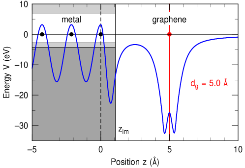
Figure 1: One-dimensional model-potential $V(z)$ for graphene/Ru(0001) at a graphene-metal distance of $d_{\rm g}=5.0$ Å. Black and red circles denote the position of Ru and C atomic layers, respectively.

$\delta V(z)$ describes the effect of higher-order image charges which arise at $0<z<d_{\rm g}$ due to infinite multiple reflections of the primary image charges at the metal surface and the graphene layer. The latter can be regarded as metallic because of the efficient screening of lateral electric fields by the sp² layer [29]. The classical image-potential between two metal surfaces with distance $d_{\rm g}$ is given by

$$V_{\rm im}(z)=-\frac{1}{4z}-\frac{1}{4(d_{\rm g}\!-\!z)}+\frac{1}{4d_{\rm g}}+\frac{1}{4d_{\rm g}}-\frac{1}{4(d_{\rm g}\!+\!z)}-\frac{1}{4(2d_{\rm g}\!-\!z)}+\ldots.$$ (2)

The first two terms in (2) represent the image-potential in atomic units caused by of the primary image-charges from each metallic surface. The following terms result from subsequent multiple reflections. By reordering, the latter can by written as

$$\delta V(z)=\frac{1}{4}\sum_{k=1}^{\infty}\frac{2}{kd_{\rm g}}-\frac{1}{kd_{\rm g}+z}-\frac{1}{(k+1)d_{\rm g}-z}\ .$$ (3)

This series converges to a net repulsive contribution. It increases the potential maximum in the center between the graphene layer and the metal surface (figure 1) from $V_{\rm im}(z\!=\!d_{\rm g}/2)=-1/d_{\rm g}$ to $V_{\rm im}(z\!=\!d_{\rm g}/2)=-\ln(2)/d_{\rm g}$, which is the classic value of the self-energy of a charged particle located in the gap between two metals [31]. For decreasing distance $d_{\rm g}$, the potential maximum is lowered. However, even at $d_{\rm g}=2.2$ Å, as found in L areas of g/Ru(0001), $V_{\rm im}(d_{\rm g}/2)=-4.54$ eV remains above the Fermi level. A simplified description of the potential between metal and graphene by an effective quantum well with a large depth of 4.8 eV below the Fermi level, as proposed by Zhang et al. [22], thus results in unrealistically large binding energies of the image-potential states. This is the main origin of the discrepancy in the identification of the first field-emission resonance observed in the STS spectra [19, 20, 21, 22].

The correction $V_{\rm\Phi}(z)$ considers the charge transfer between metal and graphene. It is approximated by a linear interpolation of the work function difference $\Delta\Phi$ between the clean metal surface and the combined system:

$$V_{\rm\Phi}(z)=\Delta\Phi\left(1-\frac{z}{d_{\rm g}}\right)\quad 0<z\leq d_{\rm g}.$$ (4)

On the basis of the model potential $V(z)$, which is depicted for the example g/Ru(0001) at a graphene separation $d_{\rm g}=5.0$ Å in figure 1, the wave function of the image-potential states and the corresponding binding energies $E_{\rm n}$ with respect to the vacuum level $E_{\rm vac}$ have been obtained by solving the one-dimensional Schrödinger equation numerically by Numerov’s method. By extending the model potential to more than $100$ Å into the metal bulk and to more than $1000$ Å into the vacuum, we made sure that the results do not depend on the system’s extension. Even if we halve these intervals, the binding energies of the image-potential states with quantum numbers $n\leq 4$ change by much less than $0.1$ meV.

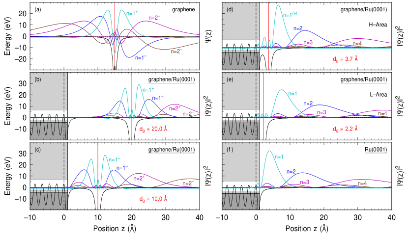
Figure 2: (a) Wave functions $\Psi(z)$ of the first two members of the symmetric ($+$) and antisymmetric ($-$) image-potential states of freestanding graphene, respectively. (b)-(f) Probability densities $|\Psi(z)|^{2}$ of the image-potential states at the graphene/Ru(0001) interface for graphene-Ru separations $d_{\rm g}$ of $20$ Å (b), $10$ Å (c), $3.7$ Å (d), H areas) and $2.2$ Å (e), L areas) and at the clean Ru(0001) surface (f). The positions of the uppermost Ru atomic layer and the graphene layer are shown by vertical black dashed and red solid lines, respectively. The solid black line depicts the one-dimensional model-potential. The projected Ru bulk band structure (gray shaded areas) has been extended up to the image-plane of the metal ($z=z_{\rm im}$).

3 Results and Discussion

Table 1 summarizes the calculated and experimental binding energies $E_{n}$ with respect to $E_{\rm vac}$ of the first two image-potential states for graphene on Ru(0001), Ir(111), and Ni(111). It shows that our model achieves a very good quantitative agreement with the experimentally observed binding energies which have been obtained by 2PPE for g/R(0001) [23] and g/Ir(111) [11]. In particular, the distinct binding energies of the ($n=1$) state in the L and H areas of g/Ru(0001) can be reproduced. Together with the predicted values for g/Ni(111), this data suggests that the binding energies of the image-potential states are strongly correlated with the graphene-metal separation $d_{\rm g}$. In order to emphasize this correlation, we will discuss in this section the systematics of the formation of image-potential states at different graphene-metal separations for the example of the strongly corrugated g/Ru(0001) because its L and H areas exhibit distinct graphene-metal separations, that are typical for strongly and weakly interacting graphene/metal systems, respectively [13].

Table 1: Calculated binding energies $E_{n}$ (eV) with respect to the vacuum level of the first two image-potential states ($n=1$) and ($n=2$) in the L and H areas of graphene/Ru(0001) and on almost flat graphene/Ir(111) and graphene/Ni(111). The results of the one-dimensional model-potential are compared to the experimental values obtained by 2PPE [23, 11]. $d_{\rm g}$ (Å) denotes the respective graphene-metal separations.

		1D-Potential		Experiment
	$d_{\rm g}$	$E_{1}$	$E_{2}$	$E_{1}$	$E_{2}$
g/Ru(0001) H [23]	3.7	0.95	0.24	$0.80\pm 0.04$	$0.18\pm 0.06$
g/Ru(0001) L [23]	2.2	0.47	0.16	$0.41\pm 0.04$	$0.18\pm 0.06$
g/Ir(111) [11]	3.4	0.88	0.23	$0.83\pm 0.02$	$0.19\pm 0.02$
g/Ni(111)	2.1	0.41	0.15

The L and H areas of g/Ru(0001) form a hexagonal moiré-superlattice with a lateral edge length of approximately $30$ Å of its $12.5\!\times\!12.5$-subunits [32, 33]. Within our one-dimensional model we can treat both areas separately because the lateral confinement due to the finite size of each area will reduce the binding energy of the image-potential states only slightly, as can be estimated from the area size of a half subunit $A\approx 420$ Å² to $\hbar^{2}\pi^{2}/2m_{\rm eff}A\approx 43$ meV, where $m_{\rm eff}=2.1\ m_{\rm e}$ with respect to the free electron mass $m_{\rm e}$ [23]. Since charge-transfer between the metal and graphene leads to a doping of graphene [29, 34], we model the work function of g/Ru(0001) as an empirical function of the graphene-Ru separation $d_{\rm g}$ by $\Phi_{\rm g/Ru}(d_{\rm g})=\Phi_{\rm g}-\xi/d_{\rm g}$, which makes it possible to vary $d_{\rm g}$ systematically for the model calculations.

Setting $\xi=1$ eV Å matches the work function $\Phi_{\rm H}=4.24$ eV in the H areas [23] as well as the $0.24$ eV lower value in the L areas [29]. For large separation, it converges to $\Phi_{\rm g}=\Phi(d_{\rm g}=\infty)=4.48$ eV [35] of freestanding graphene.

Figure 2 shows the calculated probability densities of the image-potential states for different separations $d_{\rm g}$ between the graphene layer and the Ru(0001) surface as well as for the separate systems. The corresponding binding energies are depicted in figure 3. For freestanding graphene, the two series with even ($+$) and odd ($-$) symmetry can clearly be assigned from the amplitude of their wave functions at $z=d_{\rm g}$ where the odd states have a node, whereas the even states have an antinode. The presence of the metal substrate breaks the mirror symmetry of the freestanding graphene and the parity of the image-potential is, in principle, no longer a good quantum number. At a graphene-metal separation as large as $d_{\rm g}=20$ Å, however, the influence of the substrate on the lowest members ($n=1^{+},1^{-}$) of the image-potential states is still weak due to the rather small spatial extent of their wave functions perpendicular to the surface. Therefore, their probability densities almost resemble those of freestanding graphene. We point out, that even for large $d_{\rm g}$, only image-potential states that originate from graphene and no states that are bound in the potential well formed by the image-potential of the metal and its surface barrier are found. This is related to the large difference in work function between graphene and Ru(0001) ($\Phi_{\rm Ru}=5.51$ eV [23]), which results in an additional repulsion from the Ru surface. This contributes to a reduction of the binding energies with respect to those of freestanding graphene. The latter are depicted by dashed lines in figure 3. The same argument applies for the Ir(111) ($\Phi_{\rm Ir}=5.79$ eV [11]) and the Ni(111) ($\Phi_{\rm Ni}=5.27$ eV [36]) surface. Beside the work function difference, the repulsion due to the surface barrier of the metal contributes additionally to a reduction of the binding energies with respect to freestanding graphene. At $d_{\rm g}=20$ Å, this applies particularly to the higher members ($n=2^{\pm}$, $3^{\pm}$, …) because of their more extended wave functions, which are already considerably perturbed by the repulsion due to the surface barrier. This also results in an asymmetry and phase shift of the wave functions with respect to those of freestanding graphene. The wave function of the state labeled as $n=2^{-}$ at $d_{\rm g}=20$ Å, for example, has now almost an antinode at $z=d_{\rm g}$ and more closely resembles the wave function of the ($n=3^{+}$)-state of freestanding graphene as denoted by the corresponding symbol in figure 3.

At intermediate separations, the properties of the image-potential states start to be governed by the image-potentials of both surfaces, and the attractive image-potential of the metal partly compensates for the repulsion due to the surface barrier and the work function difference. The attraction of the metal leads to a maximum of the binding energy of each state at specific separations as can be seen in figure 3. This is also reflected by the form of the wave functions shown in figure 2. At $d_{\rm g}=10$ Å, for example, the symmetric ($n=1^{+}$)-state is still almost unaffected while the more extended wave function of the ($n=1^{-}$)-state is slightly attracted towards the metal surface which results in an increase of the probability density in between the metal surface and the graphene layer compared to larger separations. For comparison we have also made simplified calculations (not shown) where we described the metal as a simple barrier without an image-potential similar to the model used in [26]. In this case, we do not observe this attraction and all image-potential states are always repelled when the graphene layer approaches the metal surface.

At small graphene-metal separations ($d_{\rm g}<5$ Å), the repulsion due to the surface barrier of the metal dominates and also the phase of the ($n=1^{-}$) wave function shifts and the latter starts to resemble that of the higher-lying ($n=2^{+}$)-state of freestanding graphene. In particular at a separation of $d_{\rm g}=3.7$ Å, which corresponds to the H areas of g/Ru(0001), the vacuum part ($z>d_{\rm g}$) of all wave functions almost resembles the corresponding part of the symmetric series of freestanding graphene. This can be regarded as a transition from the double series of image-potential states of freestanding graphene to one single series, omitting the differentiation with regard to the parity. Since only the former ($n=1^{+}$)-state maintains a certain similarity to the corresponding state on freestanding graphene, we denote this fact by writing $+$ in parentheses in the H areas. At a separation of $d_{\rm g}=2.2$ Å, which corresponds to the L areas of g/Ru(0001), all wave functions are further repelled from the metal surface. Even if the phase of the wave functions now correspond to the phase of the odd series of states on free standing graphene, the mirror symmetry has completely vanished, which is indicated by omitting the parity for the whole series. Now, all wave functions almost resemble the form of those on the clean Ru surface with one layer of atoms atop, as can be seen by comparing figure 2(e) and (f). In comparison to the clean Ru surface, however, the spatial extent of the wave functions in the vacuum is larger, which indicates a stronger decoupling from the surface. In the H areas, on the other hand, a considerable amount of the ($n=1^{(+)}$) wave function still fits in between the graphene and the Ru surface and is therefore more strongly coupled to Ru as compared to the L areas. This state is closely related to the interlayer state of graphite [5].

• 

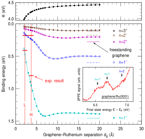
Figure 3: Work function and calculated binding energies with respect to the vacuum level of the first four members of image-potential states at graphene/Ru as a function of the separation $d_{\rm g}$ between the graphene layer and the Ru(0001) surface. Closed (open) symbols denote states with a symmetry at $z=d_{\rm g}$ which is close to the symmetry of the even (odd) image-potential states of free-standing graphene. The binding energies of the first two even ($n=1^{+}$, $2^{+}$) and odd ($n=1^{-}$, $2^{-}$) image-potential states of freestanding graphene are depicted by solid and dashed horizontal lines, respectively. The vertical lines indicate the graphene-Ru separations of the L and H areas. The inset shows the experimental 2PPE spectrum adapted from [23] which averages over a large number of L and H areas.

As depicted by the different symbols in figure 3, the change of the wave function’s character upon approaching the graphene layer to the metal surface is also reflected by the change of the binding energy with respect to the vacuum level. Whenever the binding energy of the image-potential states of the entire system becomes smaller compared to the next energetic adjacent state of freestanding graphene, the local symmetry at $z=d_{\rm g}$ is closer to the latter. At $d_{\rm g}=20$ Å, for example, the binding energies of the first, second, and third state of the entire system are larger compared to the second, third, and fourth state of freestanding graphene. Consequently, their local symmetry at $z=d_{\rm g}$ is still close to that of the first ($n=1^{+}$), second ($n=1^{-}$), and third ($n=2^{+}$) state of freestanding graphene. The energy of the fourth state of the entire system, however, is already smaller compared to the fifth state ($n=3^{+}$) of freestanding graphene. Its local symmetry at $z=d_{\rm g}$ more closely resembles the symmetry of that state and not of the fourth state ($n=2^{-}$) of freestanding graphene. The energy of this state is therefore drawn as a closed symbol which denotes states of even (local) symmetry. For decreasing graphene-metal separation, the binding energies of the image-potential states increase slightly at first due to the attractive image-potential of the metal. At separations found in real graphene/metal systems ($d_{\rm g}<5$ Å), however, the repulsion due to the surface barrier of the metal dominates and results in a rapid decrease of the binding energies upon further approach. The sequence of the relative energy spacings is, however, rather insensitive towards $d_{\rm g}$ and resembles a scaled Rydberg series with decreasing energy separation for increasing quantum number for all $d_{\rm g}$.

The absolute change of the binding energy as a function of $d_{\rm g}$ is most pronounced for the first image-potential state. It decreases from more than 1.4 eV at large $d_{\rm g}$ to 0.95 eV at the separation found in the H areas of g/Ru(0001) and finally to 0.47 eV at the separation found in the L areas. The difference between the binding energies with respect to $E_{\rm vac}$ in the H and L areas of 0.48 eV is twice as large as the difference between the local work functions of 0.24 eV [29]. The first image-potential state in the H areas has therefore a smaller energy with respect to the Fermi level $E_{\rm F}$ when compared to the the corresponding state in the L areas. This confirms the assignment of the peaks in the 2PPE spectrum of [23] which is reproduced in the inset of figure 3. This assignment is also in agreement with density functional theory (DFT) calculations by Borca et al. [19] which shows that the results of our model calculations are robust also for small distances where DFT can explicitly describe the chemical interaction between graphene and the metal. For large distances and higher quantum numbers the evolution of the binding energies with distance depicted in [19] considerably differs from our results which we attribute to the fact that DFT cannot properly consider the long-range image-force.

For the second image-potential state, the calculated difference between binding energies with respect to $E_{\rm vac}$ in the H and L areas is in the order of the difference in the local work function, which explains that these two states could not be resolved separately in the 2PPE spectra. The red horizontal lines in figure 3 depict the experimental results from [23] under consideration of the local work functions in the H and L areas, and help visualize the very good agreement between experiment and model calculation. The small deviation for the binding energy of the lowest image-potential state energy in the H areas is reduced if one considers the additional reduction of the calculated binding energy due to the lateral localization as discussed above. The localization of this state should be stronger in the H areas as deduced from the effective mass which has been found to be twice as large as the free electron mass [23].

The results of our model calculation make it also possible to qualitatively interpret the experimentally observed decay dynamics of electrons in these states, as has been investigated by time-resolved 2PPE [23]. As shown in figure 2(e), the probability densities of all image-potential states in the L areas mostly resemble those of the clean Ru(0001) surface but with some degree of decoupling, i.e. the center of gravity of the probability density is located further away from the metal into the vacuum. At first glance, this similarity to the clean Ru surface seems to be surprising. The graphene-metal separation in the L areas is, however, almost identical to the Ru-layer spacing ($d_{\rm Ru}=2.14$ Å [37]). The Ru surface covered by one metallic-like graphene overlayer therefore has similar properties with respect to the image-potential states as the extension of the Ru crystal by one more layer of Ru atoms. At the clean Ru(0001) surface, the lifetimes of electrons in the first two image-potential states of $\tau_{1}=11$ fs and $\tau_{2}=57$ fs [38, 39] are comparably short because the decay by inelastic scattering with bulk electrons is very efficient due to the high density of states of the Ru 4d bands just below the Fermi level [39]. Thus, the slightly enhanced experimental lifetimes of $\tau_{1^{-}}=16\pm 5$ fs and $\tau_{2^{-}}=85\pm 13$ fs [23] are a direct indication for a certain degree of decoupling in the L areas. In the H areas, a considerable part of the probability density of the ($n=1^{(+)}$)-state fits below the graphene layer close to the Ru surface. This enhances the electronic coupling to the Ru bulk states as is reflected by the shorter lifetime of $\tau_{1^{(+)}}=11\pm 8$ fs [23], which is identical to the value found on clean Ru(0001).

By adapting $V_{\rm m}(z)$, our model can be easily applied to the description of graphene layers on other metal substrates. With Ir(111) and Ni(111) we chose two examples that represent limiting cases of weak and strong interaction with the graphene layer, respectively. It has been shown that g/Ir(111) grows with a rather large and homogeneous separation of $d_{\rm g}=3.4$ Å [40] which is very similar to the separation found in the H areas of g/Ru(0001). Graphene and Ni(111) have almost no lattice mismatch. This results in the growth of a flat graphene layer on Ni(111), despite the strong interaction [16]. The resulting separation of about $d_{\rm g}=2.1$ Å is very similar to that found in the L areas of g/Ru(0001). Binding energies and lifetimes of the image-potential states on g/Ir(111) have been measured by 2PPE [11] and can be directly compared with the results of our model calculations. No experimental data on g/Ni(111) are available, but 2PPE results on the binding energies for the clean Ni(111) surface [36] make it possible to properly adjust the parameter of the metal potential and to predict the binding energies for the graphene covered surface. The ferromagnetic coupling of Ni results in a spin-split surface-projected band structure which is reflected by an exchange-splitting of the image-potential states. The observed splitting of $14\pm 3$ meV is, however, small compared to the linewidth and can only be observed with spin-resolved detection [36]. We therefore neglect the exchange-splitting here and use a spin-integrated surface-projected band gap extracted from [41] for our model calculations. Because the size and position of the surface-projected bulk band gap do not differ much between Ru(0001), Ir(111), and Ni(111), the calculated binding energies depend most sensitively on the graphene-metal separation $d_{\rm g}$. Consequently, the binding energies for g/Ir(111), as well as for g/Ni(111), are very similar to the results for g/Ru(0001) at the corresponding separations. As shown in table 1, the results of our model calculation for the binding energies on g/Ir(111) are in excellent agreement with the experimental data. For g/Ni(111) we predict much smaller binding energies compared to g/Ir(111). This is due to the stronger repulsion of the image-potential states at the smaller separations. The binding energies on g/Ni(111) are on the other hand comparable to those on the L areas of g/Ru(111) in correspondence to the similar separation $d_{\rm g}$.

Finally, we would like to comment on the formation of image-potential states at the interface of graphene/SiC, even if our model is not directly applicable to this semiconducting substrate. Although graphene might possess only a weak interaction to SiC, our results generally show that the shape of the image-potential states is very sensitive to the substrate induced symmetry break even for large separations due to their large spatial extent. In another 2PPE experiment on graphene/SiC(0001), Shearer et al. [42] indeed observed a single series of sharp symmetric peaks of image-potential states in agreement with data shown in [13]. Therefore, it seems rather unlikely that the experimentally found splitting of the first image-potential state on graphene/SiC [8, 10] can be interpreted as a remnant of the mirror symmetry of freestanding graphene with a small energy separation between these two states. The latter is particularly hard to understand because the approach of a flat graphene layer towards a substrate with a surface barrier does not change the relative energy spacing of adjacent states, i.e. the energy spacing between the lowest two states is always larger than the subsequent spacing because the energy sequence of the Rydberg series is at all distances dominated by the long-range image-potential.

4 Conclusion

On the basis of an analytical, one-dimensional potential, we can quantitatively describe the formation of image-potential states at the interface between a graphene layer and a metal surface by means of model calculations. By systematic variation of the graphene-metal separation, we have shown how the double Rydberg-like series of even and odd image-potential states of freestanding graphene evolves towards a single series of the compound system when a flat graphene layer is located at a distance to the metal as found in real graphene/metal systems. This transition is driven by the repulsion from the metal substrate, which increasingly reduces the mirror symmetry of freestanding graphene with decreasing separation. Even for separations found in weakly interacting systems, we find no remnant of the distinction between states of even and odd symmetry. At these intermediate separations, the first image-potential state is partly trapped between the metal and the graphene layer. It attains properties of an interfacial state. At distances found in strongly interacting systems, on the other hand, the wave functions almost resemble those of image-potential states on a clean metal surface but with a higher degree of decoupling. The repulsion of the image-potential states from the metal surface is also responsible for a strong reduction of their binding energies with decreasing graphene-metal separation. This explains the distinct differences of the experimentally observed binding energies of the first ($n=1$) image-potential states in the H and L areas of strongly corrugated g/Ru(0001). According to the respective similar separations on weakly interacting g/Ir(111) and strongly interacting g/Ni(111), we find respective comparable binding energies which are in excellent agreement with available experimental data for g/Ir(111).

Appendix A Metal Potential

For the metal part $V_{\rm m}(z)$ of our model potential we used the well-established one-dimensional potential introduced by Chulkov et al. [28]. This parameterized potential is piecewise defined along the surface normal $z$ by:

$$V_{\rm m}(z)=\cases{-A_{10}+A_{1}\cos\left(\frac{2\pi}{d_{\rm m}}z\right)&$\ z\leq 0$\\ -A_{20}+A_{2}\cos(\beta z)&$0<z\leq z_{1}$\\ -A_{3}\exp[-\alpha(z-z_{1})]&$z_{1}<z\leq z_{\rm im}$\\ \;\;\,\frac{\exp[-\lambda(z-z_{\rm im})]-1}{4(z-z_{\rm im})}&$z_{\rm im}<z$}$$ (5)

Here $d_{\rm m}$ is the layer spacing and $z=0$ corresponds to the position of the surface atom. By requiring that $V_{\rm m}(z)$ and its first derivative to be continuous at the matching points $z_{1}$ and $z_{\rm im}$, only four of the ten parameters $A_{1}$, $A_{10}$, $A_{2}$, $A_{20}$, $A_{3}$, $\alpha$, $\beta$, $\lambda$, $z_{1}$, $z_{\rm im}$ are the independent of each other. It is feasible to choose the offset $A_{1}$ and the amplitude $A_{10}$ in order to reproduce the energetic position and width of the surface-projected band gap. For Ru(0001), Ir(111) and Ni(111) (spin averaged) these have been extracted from [43, 44], [11] and [41], respectively. The parameters $A_{2}$ and $\beta$ have been used to reproduce the experimental binding energies $E_{n}$ of the image-potential states. For Ru(0001) we have fitted these parameters to the experimental binding energies $E_{1}=0.66$ eV and $E_{2}=0.19$ eV reported by Gahl et al. [38]. For Ni(111) we have used data reported by Andres et al. [36]. Due to the lack of experimental data on the image-potential states of clean Ir(111), we have estimated the binding energies by using the Rydberg formula $E_{n}=0.85\;{\rm eV}/(n+a)^{2}$ where $a$ is the quantum defect. For a $sp$-inverted band gap, the latter can be determined from the position of the vacuum energy $E_{\rm vac}$ within the projected band gap [2]. This results in $E_{1}=0.64$ eV and $E_{2}=0.18$ eV.

Table 2: Parameters of the metal part $V_{\rm m}(z)$ of the model-potentials used for Ru(0001), Ir(111), and Ni(111). The work function $\Phi$, the potential offset $A_{10}$ and amplitude $A_{1}$ are given in eV, the layer spacing $d_{\rm m}$ in Å and the parameter $\beta$ in Å^-1.

	$d_{\rm m}$	$\Phi$	$A_{10}$	$A_{1}$	$A_{2}$	$\beta$
Ru(0001)	2.138 [37]	5.51 [23]	7.436	9.400	12.70	4.3464
Ir(111)	2.217 [45]	5.79 [11]	9.511	6.188	6.50	4.6068
Ni(111)	2.035 [46]	5.27 [36]	11.259	6.503	4.91	2.3070

The parameter sets used for modelling Ru(0001), Ir(111), and Ni(111) are collected in table 2.

Appendix B Graphene Potential

• 

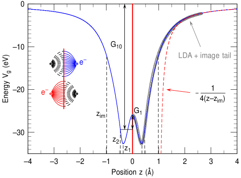
Figure 4: One-dimensional model-potential of freestanding graphene. The vertical dashed lines delimit the different definition intervals. The red dashed line represents the asymptotical form of the classical potential due to the image-charges of both surfaces (inset). Gray circles depict the ”LDA+image tail” potential which has been extracted from figure 1 of [5].

Our analytical approximation of the ”LDA+image tail” hybrid potential of Silkin et al. [5] for the description of freestanding graphene is inspired by the definition of the metal potential with omission of the bulk part:

$$V_{\rm g}(z)=\cases{-G_{10}+G_{1}\cos(\beta_{1}|z|)&$0<|z|\leq|z_{1}|$\\ -G_{20}-G_{2}\cos[\beta_{2}(|z|-|z_{1}|)]&$|z_{1}|<|z|\leq|z_{2}|$\\ -G_{3}\exp[-\alpha(|z|-|z_{2}|)]&$|z_{2}|<|z|\leq|z_{\rm im}|$\\ \;\;\,\frac{\exp[-\lambda(|z|-|z_{\rm im}|)]-1}{4(|z|-|z_{\rm im}|)}&$|z_{\rm im}|<|z|$.}$$ (6)

As shown in figure 4, $V_{\rm g}(z)$ is symmetric in the $z$-direction with respect to the graphene layer at $z=0$ and converges to the classical image-potential for large distances $|z|$. Again, only four of the twelve parameters $z_{1}$, $z_{2}$, $z_{\rm im}$, $G_{1}$, $G_{10}$, $G_{2}$, $G_{20}$, $G_{3}$, $\beta_{1}$, $\beta_{2}$, $\alpha$, and $\lambda$ are independent if we require $V_{\rm g}(z)$ to be continuously differentiable at the matching points $z_{1}$, $z_{2}$, and $z_{\rm im}$. We choose the potential offset $G_{10}=\Phi_{g}+V_{0}$, the amplitude $G_{1}$, and the inverse widths $\beta_{1}$ and $\beta_{2}$ to fit $V_{\rm g}(z)$ to the ”LDA+image tail” hybrid potential for a matching point between LDA potential and image-tail of $z_{0}=3$ a.u. The best fit is shown as solid line in figure 4. It has been achieved with $G_{1}=3.336$ eV, $G_{10}=29.3465$, $\beta_{1}=8.7266$ and $\beta_{2}=14.8353$.

The binding energies $E^{\pm}_{n}$ of the symmetric and antisymmetric image-potential states calculated with these parameters are listed in table 3. They agree well with those calculated using the ”LDA+image tail” hybrid potential for $z_{0}=3$ a.u. [5] The two equivalent positions of the image-planes of $z_{\rm im}=\pm 0.99$ Å, which result from the chosen parameters, are almost coincident with the spatial extent of the polarizable conjugated $\pi$-system [5].

Table 3: Binding energies $E_{n^{\pm}}$ (eV) calculated with the one-dimensional model potential and the ”LDA+image tail” hybrid potential [5], respectively.

	$E_{1^{+}}$	$E_{1^{-}}$	$E_{2^{+}}$	$E_{2^{-}}$
1D-Potential	1.46	0.60	0.28	0.18
LDA+image tail	1.47	0.72	0.25	0.19

The screening of electric fields by the metal as well as the graphene layer is taken into account by cutting the corresponding image tail of $V_{\rm m}(z)$ and $V_{\rm g}(z)$ at the respective opposite surface ($V_{\rm m}(z)=0$ for $z>d_{\rm g}$ and $V_{\rm g}(z)=0$ for $z<0$). Together with the corrections $\delta V(z)$ and $V_{\rm\Phi}(z)$, this results in a discontinuity of the total model potential $V(z)$ at $z=0$ and $z=d_{\rm g}$. The discontinuity is compensated by increasing the amplitudes of the respective cosine oscillation of the metal potential $V_{\rm m}$ (5) and the graphene potential $V_{\rm g}$ (6).

References

References

- [1] Echenique P M and Pendry J B 1978 J. Phys. C 11 2065
- [2] Fauster T and Steinmann W 1995 Photonic probes of surfaces Electromagnetic Waves: Recent Developments in Research vol 2 ed Halevi P (Amsterdam: North-Holland) pp 347
- [3] Höfer U, Shumay I L, Reuß C, Thomann U, Wallauer W and Fauster T 1997 Science 277 1480
- [4] Höfer U and Echenique P M 2015 Surf. Sci. in press
- [5] Silkin V M, Zhao J, Guinea F, Chulkov E V, Echenique P M and Petek H 2009 Phys. Rev. B 80 121408
- [6] Wintterlin J and Bocquet M L 2009 Surf. Sci. 603 1841
- [7] Emtsev K V, Bostwick A, Horn K, Jobst J, Kellogg G L, Ley L, McChesney J L, Ohta T, Reshanov S A, Roehrl J, Rotenberg E, Schmid A K, Waldmann D, Weber H B and Seyller T 2009 Nature Materials 8 203
- [8] Bose S, Silkin V M, Ohmann R, Brihuega I, Vitali L, Michaelis C H, Mallet P, Veuillen J Y, Schneider M A, Chulkov E V, Echenique P M and Kern K 2010 New J. Phys. 12 023028
- [9] Sandin A, Pronschinske A, Rowe J E and Dougherty D B 2010 Appl. Phys. Lett. 97 113104
- [10] Takahashi K, Imamura M, Yamamoto I, Azuma J and Kamada M 2014 Phys. Rev. B 89 155303
- [11] Niesner D, Fauster T, Dadap J I, Zaki N, Knox K R, Yeh P C, Bhandari R, Osgood R M, Petrović M and Kralj M 2012 Phys. Rev. B 85 081402
- [12] Nobis D, Potenz M, Niesner D and Fauster T 2013 Phys. Rev. B 88 195435
- [13] Niesner D and Fauster T 2014 J. Phys.: Condens. Matter. 26 393001
- [14] Craes F, Runte S, Klinkhammer J, Kralj M, Michely T and Busse C 2013 Phys. Rev. Lett. 111(5) 056804
- [15] Preobrajenski A B, Ng M L, Vinogradov A S and Mårtensson N 2008 Phys. Rev. B 78 073401
- [16] Parreiras D E, Soares E A, Abreu G J P, Bueno T E P, Fernandes W P, de Carvalho V E, Carara S S, Chacham H and Paniago R 2014 Phys. Rev. B 90 155454
- [17] Wang B, Bocquet M L, Marchini S, Günther S and Wintterlin J 2008 Phys. Chem. Chem. Phys. 10(24) 3530
- [18] Moritz W, Wang B, Bocquet M L, Brugger T, Greber T, Wintterlin J and Günther S 2010 Phys. Rev. Lett. 104 136102
- [19] Borca B, Barja S, Garnica M, Sánchez-Portal D, Silkin V M, Chulkov E V, Hermanns C F, Hinarejos J J, Vázquez de Parga A L, Arnau A, Echenique P M and Miranda R 2010 Phys. Rev. Lett. 105 036804
- [20] Zhang H G and Greber T 2010 Phys. Rev. Lett. 105 219701
- [21] Borca B, Barja S, Garnica M, Sánchez-Portal D, Silkin V M, Chulkov E V, Hermanns C F, Hinarejos J J, Vázquez de Parga A L, Arnau A, Echenique P M and Miranda R 2010 Phys. Rev. Lett. 105 219702
- [22] Zhang H G, Hu H, Pan Y, Mao J H, Gao M, Guo H M, Du S X, Greber T and Gao H J 2010 J. Phys.: Condens. Matter. 22 302001
- [23] Armbrust N, Güdde J, Jakob P and Höfer U 2012 Phys. Rev. Lett. 108 056801
- [24] Blase X, Rubio A, Louie S G and Cohen M L 1995 Phys. Rev. B 51 6868
- [25] Cuong N T, Otani M and Okada S 2014 J. Phys.: Condens. Matter. 26 135001
- [26] de Andres P L, Echenique P M, Niesner D, Fauster T and Rivacoba A 2014 New J. Phys. 16 023012
- [27] Pagliara S, Tognolini S, Bignardi L, Galimberti G, Achilli S, Trioni M I, van Dorp W F, Ocelík V, Rudolf P and Parmigiani F 2015 Phys. Rev. B 91 195440
- [28] Chulkov E V, Silkin V M and Echenique P M 1999 Surf. Sci. 437 330
- [29] Brugger T, Günther S, Wang B, Dil J H, Bocquet M L, Osterwalder J, Wintterlin J and Greber T 2009 Phys. Rev. B 79 045407
- [30] Varykhalov A, Sánchez-Barriga J, Shikin A M, Biswas C, Vescovo E, Rybkin A, Marchenko D and Rader O 2008 Phys. Rev. Lett. 101(15) 157601
- [31] Sols F and Ritchie R H 1987 Phys. Rev. B 35 9314
- [32] Martoccia D, Willmott P R, Brugger T, Bjorck M, Günther S, Schlepütz C M, Cervellino A, Pauli S A, Patterson B D, Marchini S, Wintterlin J, Moritz W and Greber T 2008 Phys. Rev. Lett. 101 126102
- [33] Martoccia D, Bjorck M, Schlepütz C M, Brugger T, Pauli S A, Patterson B D, Greber T and Willmott P R 2010 New J. Phys. 12 043028
- [34] Sutter P, Hybertsen M S, Sadowski J T and Sutter E 2009 Nano Lett. 9 2654
- [35] Giovannetti G, Khomyakov P A, Brocks G, Karpan V M, van den Brink J and Kelly P J 2008 Phys. Rev. Lett. 101 026803
- [36] Andres B, Weiss P, Wietstruk M and Weinelt M 2015 J. Phys.: Condens. Matter. 27 015503
- [37] Pelzer T, Ceballos G, Zbikowski F, Willerding B, Wandelt K, Thomann U, Reuss C, Fauster T and Braun J 2000 J. Phys.:Condens. Matter. 12 2193
- [38] Gahl C 2004 Elektronentransfer- und Solvatisierungsdynamik in Eis adsorbiert auf Metalloberflächen Phd thesis Freie Universität Berlin
- [39] Berthold W, Höfer U, Feulner P and Menzel D 2000 Chem. Phys. 251 123
- [40] Busse C, Lazić P, Djemour R, Coraux J, Gerber T, Atodiresei N, Caciuc V, Brako R, N’Diaye A T, Blügel S, Zegenhagen J and Michely T 2011 Phys. Rev. Lett. 107(3) 036101
- [41] Schuppler S, Fischer N, Fauster T and Steinmann W 1992 Phys. Rev. B 46 13539
- [42] Shearer A J, Johns J E, Caplins B W, Suich D E, Hersam M C and Harris C B 2014 Appl. Phys. Lett. 104 231604
- [43] N. A. W. Holzwarth and J. R. Chelikowsky, 1985 Solid State Commun. 53 171
- [44] Lindroos M, Pfnür and Menzel D 1986 Phys. Rev. B 33 6684
- [45] Needs R J and Mansfield M 1989 J. Phys.: Condens. Matter. 1 7555
- [46] von Bachtelder F W and Raeuchle R F 1954 Acta Cryst. 7 464