Pseudo-Riemannian Universe from Euclidean bulk

Abstract

I develop the idea that our world is a brane-like object embedded in Euclidean bulk. In its ground state, the brane constituent matter is assumed to be homogeneous and isotropic, and of negligible influence on the bulk geometry. The analysis of this paper is model independent, in the sense that action functional of bulk fields is not specified. Instead, the behavior of the brane is derived from the universally valid conservation equation of the bulk stress tensor. The present work studies the behavior of a $3$-sphere in the $5$-dimensional Euclidean bulk. The sphere is made of bulk matter characterized by the equation of state $p=\alpha\rho$. It is shown that stability of brane vibrations requires $\alpha<0$. Then, the stable brane perturbations obey Klein-Gordon-like equation with an effective metric of Minkowski signature. The argument is given that it is this effective metric that is detected in physical measurements. The corresponding effective Universe is analyzed for all the values of $\alpha<0$. In particular, the effective metric is shown to be a solution of Einstein’s equations coupled to an effective perfect fluid. The effective energy density and pressure at the present epoch are calculated. So are the age of the Universe, and the effective cosmological constant. All the results are presented in two tables. As an illustration, one simple choice of the brane constituent matter is studied in detail.

I Introduction

The mainstream braneworld physics, which has extensively been developed after the seminal work of Randall and Sundrum RS1 ; RS2 , typically employs pseudo-Riemannian bulks. In this paper, I am investigating the idea that our world is a domain wall embedded in a higher dimensional Euclidean space. This is motivated by the observation that Euclidean bulk may improve stability properties of the brane Universe. Indeed, it is straightforwardly verified that spherical branes embedded in Minkowski bulk are unstable, irrespectively of the nature of the brane constituent matter. In particular, the dynamics of Nambu-Goto $3$-sphere is burdened with the presence of tachyons.

The general idea behind this line of research is an attempt to obtain the observed physics as a physics of brane vibrations. This is a kind of geometrization program, in which observable matter is identified with disturbances of the braneworld vacuum solution. In this respect, it resembles the string theory. The brane vibrations are expected to model physical fields the same way as string vibrations model elementary particles.

Before I continue, let me explain why I believe this geometrization program may work. I start with the observation that our physical fields can be seen as a $4$-dimensional surface embedded in a higher-dimensional bulk. Indeed, the parametric form of a $4$-surface in a $D$-dimensional bulk is defined by $D$ functions of $4$ coordinates. If the $4$-surface is interpreted as the trajectory of a $3$-brane, the field equations become the brane world-sheet equations. This way, the behavior of physical fields becomes the behavior of a $3$-brane. In a perturbative analysis, the physical fields are associated with vibrations of the brane vacuum. Then, the reparametrization invariant world-sheet equations describe $D-4$ field components. This way, every conventional field theory can be rewritten in terms of brane vibrations. An early attempt along these lines is the construction of geodetic brane gravity b1 ; b2 ; b3 ; b4 . With this thought in mind, I choose the simplest possible scenario to illustrate this idea.

In this paper, I shall study small perturbations of a simple braneworld vacuum. I begin with the assumption that the brane is made of matter fields that live in a $5$-dimensional Euclidean bulk. The analysis is model independent, in the sense that action functional of the bulk matter is not specified. Instead, I use the universally valid conservation equations of the stress tensor. The problem with this approach is that the brane interior may have its own degrees of freedom. This may compromise the original idea that observable matter stems from the brane vibrations alone. To prevent this, I shall assume that the brane interior is hard to excite. This can always be achieved by a proper choice of the bulk matter. The needed ground state of the brane is searched for in the form of a homogeneous and isotropic $3$-sphere. This way, my program reduces to the construction of a braneworld Universe. (The idea to describe Universe as a spherical shell has first been considered in a1 ; a2 ; a3 , and more recently in a4 ; a5 .) Let me summarize the basic assumptions of this program:

• The arena for my considerations is a higher-dimensional space called bulk.

• The dynamics of bulk fields is governed by a diffeomorphism invariant action functional.

• Diffeomorphism invariance implies the existence of the conserved stress tensor.

• The bulk action is assumed to possess a brane-like kink solution. Such a kink resembles a 4-dimensional surface called world-sheet.

• The presented analysis is model independent, in the sense that the action is not explicitly specified. Instead, the world-sheet equations are derived from the universally valid conservation equations of the bulk stress tensor.

• The brane is assumed to have negligible influence on the bulk geometry. Consequently, the bulk geometry is well approximated by the flat Euclidean space.

• For simplicity, the considerations of this work are restricted to the 5-dimensional bulk.

I start with the conservation equation of the bulk stress tensor,

$$\nabla_{\nu}T^{\mu\nu}=0\,,$$ (1)

and apply it to bulk fields that form a brane-like kink configuration called world-sheet. Throughout the paper, it is assumed that the brane has negligible influence on the bulk geometry. In other words, I work in the probe matter approximation. (An early model of probe brane-worlds has been proposed in b1 , and later developed in b2 ; b3 ; b4 .) The derivation of the manifestly covariant world-sheet equations is developed in VV1 ; VV2 , as a generalization of the Mathisson-Papapetrou method for point-like matter M ; P . According to this, the stress tensor $T^{\mu\nu}(x)$, which is well localized around the $(p+1)$-dimensional surface ${\cal M}$ in a $D$-dimensional bulk, has an expansion as a series of $\delta$-function derivatives. For infinitely thin branes of Euclidean nature, this multipole expansion reduces to

$$T^{\mu\nu}=\int_{{\cal M}}d^{p+1}\xi\sqrt{\gamma}\,M^{\mu\nu}\frac{\delta^{(D)}(x-z)}{\sqrt{g}}\,.$$ (2)

The surface ${\cal M}$ is defined by the equation $x^{\mu}=z^{\mu}(\xi)$, where $\xi^{a}$ are the surface coordinates, and $M^{\mu\nu}(\xi)$ are free coefficients. The surface coordinate vectors $u_{a}^{\mu}\equiv\partial z^{\mu}/\partial\xi^{a}$ define the surface induced metric $\gamma_{ab}\equiv g_{\mu\nu}u_{a}^{\mu}u_{b}^{\nu}$. The bulk metric is denoted by $g_{\mu\nu}(x)$.

The decomposition (2) is used as an ansatz for solving the conservation equation (1). This has already been done in VV2 , where manifestly covariant $p$-brane world-sheet equations and boundary conditions have been derived. These equations determine the behavior of the embedding functions $z^{\mu}(\xi)$, and the coefficients $M^{\mu\nu}(\xi)$. Skipping the details of the calculation, I shall display the final result. The equation (1) leads to the world-sheet equations

$${P_{{\scriptscriptstyle\perp}}}\vphantom{P}^{\mu}_{\lambda}M^{\nu\lambda}=0\,,\qquad\nabla_{a}\left(M^{\mu\nu}u^{a}_{\nu}\right)=0\,,$$

where ${P_{{\scriptscriptstyle\perp}}}\vphantom{P}^{\mu}_{\nu}\equiv\delta^{\mu}_{\nu}-u_{a}^{\mu}u^{a}_{\nu}$ is the orthogonal projector to the world-sheet, and $\nabla_{a}$ stands for the total covariant derivative that acts on both types of indexes. The boundary conditions are trivially satisfied. The equation ${P_{{\scriptscriptstyle\perp}}}\vphantom{P}^{\mu}_{\lambda}M^{\nu\lambda}=0$ tells us that $M^{\mu\nu}$ coefficients lack the orthogonal components. Therefore, their general form is

$$M^{\mu\nu}=m^{ab}u^{\mu}_{a}u^{\nu}_{b}\,,$$

where $m^{ab}(\xi)$ are the residual free coefficients. In terms of $m^{ab}$, the brane world-sheet equations are rewritten as

$$\nabla_{a}\left(m^{ab}u^{\mu}_{b}\right)=0\,.$$ (3)

It is straightforward to verify that the equations (3) imply the covariant conservation law

$$\nabla_{a}m^{ab}=0\,.$$

For this reason, the coefficients $m^{ab}$ will be referred to as the brane stress tensor.

The results obtained in this paper are summarized as follows. (a) The ground state stress tensor $m^{ab}$ is characterized by the generic equation of state $p=p(\rho)$, independently of the nature of the brane constituent matter. In the sector of small $\rho$, this equation takes the widely exploited form $p=\alpha\rho$. (b) The stability analysis is presented. I demonstrate that the condition $\alpha<0$ is a universal necessary condition to ensure stable ground state of the brane Universe. With this condition satisfied, the infinitesimal brane vibrations obey Klein-Gordon-like equation with an effective metric of Minkowski signature. If these vibrations are identified with the observable matter, the obtained effective metric defines the observed pseudo-Riemannian geometry. The corresponding effective Universe is investigated for a range of values of $\alpha<0$. It is shown that the effective metric, coupled to an effective perfect fluid, becomes a solution of Einstein’s equations. This way, the effective Universe is rewritten in terms of the standard general relativistic (GR) cosmology. The present time values of the effective energy density and pressure are calculated along with the effective cosmological constant and the age of the Universe. The results are presented in two tables. (c) As an example, the brane made of an incompressible fluid is studied in detail. The stability of both, brane vibrations and brane interior, is proven for all $\alpha\leq-1/3$. (d) It is demonstrated that bulk conservation equations do not allow braneworlds of finite lifetime. In particular, the Big Bang cosmology is not supported by the typical braneworld concept. I ague, however, that these solutions are perfectly legitimate if restricted to sectors which are not close to singularities.

The conventions used throughout the paper are the following. Greek indices $\mu,\nu,\dots$ are the bulk indices, and run over $0,1,2,3,4$. Latin indices $a,b,\dots$ are the braneworld indices, and run over $0,1,2,3$. The coordinates of the bulk and brane are denoted by $x^{\mu}$ and $\xi^{a}$, respectively. The bulk metric is the flat Euclidean metric $\delta_{\mu\nu}$, and the induced braneworld metric is $\gamma_{ab}(\xi)$. The signature convention is defined by $\mathop{\rm diag}\nolimits(+,+,\dots,+)$, and the indices are raised using the inverse metrics $\delta^{\mu\nu}$ and $\gamma^{ab}$.

II Ground state solution

Supported by astronomical observations, the ground state of the Universe is conventionally considered spatially homogeneous and isotropic. This leaves us with a limited choice of ground state branes and allowed stress-energy tensors. In this paper, the ground state brane is assumed to be a $3$-sphere embedded in the $5$-dimensional Euclidean space. Its world-sheet $x^{\mu}=z^{\mu}(\xi)$ is defined by

$$z^{0}=t,\ z^{1}=\ell(t)\cos\psi,\ z^{2}=\ell(t)\sin\psi\cos\theta,$$

$$z^{3}=\ell(t)\sin\psi\sin\theta\cos\phi\,,$$ (4)

$$z^{4}=\ell(t)\sin\psi\sin\theta\sin\phi\,,$$

where the identification $\xi^{0}\equiv t$, $\xi^{1}\equiv\psi$, $\xi^{2}\equiv\theta$, $\xi^{3}\equiv\phi$ is used. The $t$ coordinate takes values on the whole real axis, and $\psi,\theta,\phi$ are the standard angular coordinates of the $3$-sphere ($\psi\in[0,\pi]$, $\theta\in[0,\pi]$, $\phi\in[0,2\pi]$). Then, one readily calculates the coordinate vectors $u^{\mu}_{a}\equiv\partial z^{\mu}/\partial\xi^{a}$, and the induced metric $\gamma_{ab}\equiv\delta_{\mu\nu}u^{\mu}_{a}u^{\nu}_{b}$. The induced metric is read from

$$ds^{2}=\big{(}\dot{\ell}^{2}+1\big{)}dt^{2}+\ell^{2}\left[d\psi^{2}+\sin^{2}\psi\left(d\theta^{2}+\sin^{2}\theta\,d\phi^{2}\right)\right],$$ (5)

where $\dot{\ell}\equiv d\ell/dt$. The radius $\ell(t)$ is an undetermined variable of the brane equations (3).

The general form of the homogeneous and isotropic world-sheet stress tensor $m^{ab}$ is

$$m^{ab}=\left(\begin{array}[]{cc}\rho\gamma^{00}&0\\ 0&p\gamma^{\alpha\beta}\\ \end{array}\right),$$ (6)

where $\alpha,\beta=1,2,3$, and the variables $\rho=\rho(t)$ and $p=p(t)$ depend on $t$ only. It is easily checked that only two out of five equations (3) are independent, which is insufficient to determine the three unknown variables $\rho$, $p$ and $\ell$. One needs to further specify the nature of the brane constituent matter. In what follows, I shall demonstrate that the equation of state $p=\alpha\rho$, which is conventionally imposed by hand, is in fact, universal in the sector of small $\rho$. Indeed, the assumption of spatial homogeneity ensures that $\rho=\rho(t)$ and $p=p(t)$, which is nothing but the parametric form of the relation $p=p(\rho)$. When expanded in a power series around $\rho=0$, it takes the form

$$p=\alpha_{0}+\alpha_{1}\rho+\alpha_{2}\rho^{2}+\cdots\,,$$

which reduces to $p=\alpha_{0}+\alpha_{1}\rho$ in the sector of small $\rho$. In the conventional physics, the condition $\rho=0$ implies $p=0$, and therefore, $\alpha_{0}=0$. Although my considerations in this section are not conventional, it will be shown later that they lead to a conventional effective Universe. For this reason, the condition $\alpha_{0}=0$ is needed in my considerations, too. Thus, I am left with the approximate equation of state

$$p=\alpha\rho$$ (7)

applicable in the sector of small $\rho$. Exotic equations of state, which can not be expanded in a power series around $\rho=0$, can still be approximated by (7) in the close vicinity of $\rho=0$. Indeed, in the limit $\rho\to 0$, $\alpha\to\infty$, the exotic equations of state are practically indistinguishable from (7).

The world-sheet equations (3) with the equation of state (7) are straightforwardly solved. As it turns out, only two out of five equations are independent. The equation

$$\frac{\dot{\rho}}{\rho}=3\left(\alpha-1\right)\frac{\dot{\ell}}{\ell}$$

follows from the conservation equation of the brane stress tensor $m^{ab}$, while

$$\frac{d}{dt}\left(\frac{\ell^{3\alpha}}{\displaystyle\sqrt{1+\dot{\ell}^{2}}}\right)=0$$

is derived from the zero component of the world-sheet equations (3). In what follows, the coordinate $t$ will be replaced by $\eta$, as defined by

$$\sqrt{1+\dot{\ell}^{2}}\,dt=\ell d\eta\,.$$ (8)

In terms of $\eta$, the induced metric takes the form

$$ds^{2}=R^{2}(\eta)\left[d\eta^{2}+d\psi^{2}+\sin^{2}\psi\left(d\theta^{2}+\sin^{2}\theta\,d\phi^{2}\right)\right],$$ (9)

and the solution for $R(\eta)\equiv\ell(t(\eta))$ reads

$$R=R_{0}\exp\left(\frac{\eta}{\eta_{0}}\right)\quad{\rm for}\quad\alpha=0\,,$$ (10a)

$$R=R_{0}\big{[}\cosh(3\alpha\eta)\big{]}^{\frac{1}{3\alpha}}\quad{\rm for}\quad\alpha\neq 0\,.$$ (10b)

The solution for $\rho\equiv\rho(t(\eta))$ is

$$\rho=\rho_{0}\left(\frac{R}{R_{0}}\right)^{3\left(\alpha-1\right)}\,.$$ (11)

The parameters $\rho_{0}$, $R_{0}$ and $\eta_{0}$ are integration constants.

The behavior of the $3$-sphere can also be parametrized by the proper parameter $\tau$. It is defined by $d\tau=R\,d\eta$ whereupon the induced metric takes the form

$$ds^{2}=d\tau^{2}+a^{2}\left[d\psi^{2}+\sin^{2}\psi\left(d\theta^{2}+\sin^{2}\theta\,d\phi^{2}\right)\right].$$

The $\tau$ dependence of the radius $a(\tau)\equiv R(\eta(\tau))$ for $\alpha>0$ and $\alpha<0$ is shown in Fig. 1. For $\alpha=0$, the radius $a(\tau)$ is a linear function of $\tau$.

Figure 1: Behavior of the brane Universe.

Let me remind you that the above solutions are valid only in the sector of small $\rho$. If $R_{0}$ is big enough, this does not influence the case $\alpha>0$, but definitely excludes the vicinity of singular points in the case $\alpha<0$.

At the end of this section, I want to draw the reader’s attention to the fact that the obtained vacuum solution violates the equality of all directions inherited from the Euclidean bulk. Indeed, the geometry (9), with $R(\eta)$ given by (10), is homogeneous and isotropic in three compact directions, but not in the $\eta$ direction. As a consequence, the world-sheet is endowed with a privileged direction. This is exactly the origin of the effective Lorenzian metric derived in the next section. The asymmetry of the vacuum solution itself, on the other hand, is a consequence of the assumed compactness of the $3$-brane. In such a case, the brane must be infinite in the remaining direction. Indeed, it is straightforward to verify that the conservation equation (1) forbids fully compact world-sheets. In simple terms, matter can not be created out of nothing. Therefore, the equality of all directions on the world-sheet is violated already by the fact that the world-sheet has only one infinite dimension.

III Stability analysis

In this section, I shall examine the stability of the solution (10) against small perturbations of the brane. Without loss of generality, the brane perturbations are defined by

$$\delta x^{\mu}=\epsilon\,n^{\mu},$$

where $n^{\mu}$ is the unit normal to the ground state wold-sheet, and $\epsilon=\epsilon(\xi)$. This way, we are left with only one component of the brane perturbations. This is a consequence of the fact that 4-dimensional world-sheet $x^{\mu}(\xi)$ has only one orthogonal direction in the considered 5-dimensional bulk. The other variable is the variation of the brane stress tensor $\delta m^{ab}$. In the model independent approach of this paper, $\delta m^{ab}$ is not fully specified.

Let me start with rewriting the world-sheet equations (3) in the equivalent form

$$m^{ab}K^{\mu}_{ab}=0\,,\qquad\nabla_{a}m^{ab}=0\,,$$

where $K^{\mu}_{ab}$ stands for the extrinsic curvature of the brane world-sheet,

$$K^{\mu}_{ab}\equiv\nabla_{a}u^{\mu}_{b}\,.$$

It is straightforwardly checked that the bulk vectors $K^{\mu}_{ab}$ are orthogonal to the world-sheet. In the 5-dimensional bulk considered in this paper, this implies the decomposition

$$K^{\mu}_{ab}=n^{\mu}K_{ab}\,.$$

In terms of the extrinsic curvature $K^{\mu}_{ab}$ and the world-sheet connection $\Gamma^{a}{}_{bc}$, the perturbed world-sheet equations read:

$$K^{\mu}_{ab}\,\delta m^{ab}+m^{ab}\delta K^{\mu}_{ab}={\cal O}_{2}\,,$$

$$\nabla_{a}\delta m^{ab}+m^{cb}\delta\Gamma^{a}{}_{ca}+m^{ac}\delta\Gamma^{b}{}_{ca}={\cal O}_{2}\,.$$

The variation $\delta\Gamma^{a}{}_{bc}$ is easily calculated once the variation of the induced metric is known. The needed expressions for $\delta\gamma_{ab}$ and $\delta K^{\mu}_{ab}$ are obtained straightforwardly. They read:

$$\delta\gamma_{ab}=-2K_{ab}\epsilon\,,$$

$$\delta K^{\mu}_{ab}=n^{\mu}\left(\nabla_{a}\nabla_{b}-K^{c}{}_{a}K_{cb}\right)\epsilon-u^{c\mu}K_{ab}\nabla_{c}\epsilon\,.$$

With this, the perturbed world-sheet equations take the form

$$m^{ab}\left(\nabla_{a}\nabla_{b}-K^{c}{}_{a}K_{cb}\right)\epsilon+K_{ab}\,\delta m^{ab}={\cal O}_{2}\,,$$ (12)

$$\begin{array}[]{rcl}&&\displaystyle\left(m^{ac}\,\nabla^{b}K_{ac}+m^{bc}\,\nabla_{c}K^{a}{}_{a}\right)\epsilon+{}\\ &&\displaystyle\left(2m^{ac}K^{b}{}_{a}+m^{bc}K^{a}{}_{a}\right)\nabla_{c}\epsilon-\nabla_{a}\,\delta m^{ab}={\cal O}_{2}\,.\end{array}$$ (13)

In the linear approximation I work with, the tensors $m^{ab}$ and $K_{ab}$ take their vacuum values, and are straightforwardly calculated. Precisely, the vacuum form of $m^{ab}$ is given by (6), (7) and (11) of the preceding section, while nonzero components of $K_{ab}$ read:

$$K_{00}=3\alpha\,R\left(\frac{R_{0}}{R}\right)^{3\alpha},\quad K_{\alpha\beta}=-\frac{1}{R}\left(\frac{R_{0}}{R}\right)^{3\alpha}\gamma_{\alpha\beta}\,.$$

With given $m^{ab}$ and $K_{ab}$, one still lacks enough information to solve the perturbation equations. Indeed, the form of the variation $\delta m^{ab}$ remains unknown in the model independent approach of the present work. The needed information is hidden in the structure of the brane constituent matter.

In what follows, I shall restrain from specifying the model Lagrangian of the world-sheet matter. Instead, I shall only assume that world-sheet matter does not couple to metric derivatives. Among matter fields that satisfy this assumption is commonly used scalar field, but also electromagnetic and Yang-Mills fields. With these constituent fields, the term $\delta m^{ab}$ lacks $\epsilon$ derivatives. Thus, the kinetic term of the equation (12) is not influenced by $\delta m^{ab}$.

The structure of the kinetic term is best seen if the dependence on $\epsilon$ derivatives is explicitly shown. This is achieved by rewriting the equation (12) in the form

$${\begin{array}[]{rcl}\displaystyle\frac{\rho}{R^{2}}\bigg{[}&&\displaystyle\ddot{\epsilon}+\alpha\triangle\epsilon+\left(3\alpha-1\right)\frac{\dot{R}}{R}\,\dot{\epsilon}\\ &&\displaystyle{}-\alpha\left(\alpha+\frac{1}{3}\right)R^{2}\left(K^{\alpha}_{\alpha}\right)^{2}\epsilon\bigg{]}+K_{ab}\,\delta m^{ab}={\cal O}_{2}\,,\end{array}}$$

where $\triangle$ stands for the Laplacian of the unit $3$-sphere. To simplify this expression, I introduce the auxiliary metric $\tilde{\gamma}_{ab}$ defined by

$$d\tilde{s}^{2}\equiv-A\left\{d\eta^{2}+\frac{1}{\alpha}\Big{[}d\psi^{2}+\sin^{2}\psi\left(d\theta^{2}+\sin^{2}\theta\,d\phi^{2}\right)\Big{]}\right\}.$$ (14)

The shorthand notation

$$A\equiv R_{0}^{2}\left(\frac{R}{R_{0}}\right)^{3\alpha-1}$$

is introduced for convenience. Using this auxiliary metric, one can construct the box operator $\tilde{\Box}\equiv\tilde{\gamma}^{ab}\,\tilde{\nabla}_{a}\tilde{\nabla}_{b}$. It is checked that its action on the scalar $\epsilon(\xi)$ reduces to

$$\tilde{\Box}\,\epsilon\equiv-\frac{1}{A}\bigg{[}\ddot{\epsilon}+\alpha\triangle\epsilon+\left(3\alpha-1\right)\frac{\dot{R}}{R}\,\dot{\epsilon}\bigg{]}.$$

Now, it is seen that the kinetic term of the above word-sheet equation has the form $\tilde{\Box}\,\epsilon$. The complete perturbation equation (12) is rewritten as

$$\left[\tilde{\Box}+3\alpha\left(3\alpha+1\right){B}\right]\epsilon-{C}K_{ab}\,\delta m^{ab}={\cal O}_{2}\,,$$ (15)

where the notation

$${B}\equiv\frac{1}{R^{2}_{0}}\left(\frac{R_{0}}{R}\right)^{9\alpha-1},\quad{C}\equiv\frac{1}{\rho_{0}}\left(\frac{R_{0}}{R}\right)^{6(\alpha-1)}$$

is introduced for convenience. The unknown variation $\delta m^{ab}$ can contribute to the mass and source terms of the equation (15), but it can not modify the kinetic term $\tilde{\Box}\epsilon$. Therefore, the auxiliary metric $\tilde{\gamma}_{ab}$ must have Minkowski signature to prevent the instability of the vacuum solution $\epsilon=0$. It follows then that vacuum stability requires negative $\alpha$.

• Vacuum stability requires $\alpha<0$.

It should be noted that this is just a necessary condition, as the full stability also requires a proper sign of the mass term, which can not be fully determined without the knowledge of $\delta m^{ab}$. Besides, the equation (15) can also have a source. Its origin is the brane matter, whose dynamics is only partially determined by the equation (13). For the full stability analysis, one needs a model Lagrangian of the world-sheet matter. In Sec. V, a specific example of the brane constituent matter is considered in detail. In particular, the brane made of an incompressible perfect fluid is shown to have stable dynamics whenever $\alpha\leq-1/3$.

Let me conclude this section with the important observation that the auxiliary metric $\tilde{\gamma}_{ab}$ is, in fact, the metric which is detected in physical measurements. Indeed, the spacetime metric is always determined by measuring behavior of test matter in curved geometry. In my geometric approach, the observable matter is identified with brane vibrations. As a consequence, the scalar $\epsilon(\xi)$ is the only detectable matter in the case under consideration. Its dynamics is governed by the Klein-Gordon type equation (15). This means that the observer that detects $\epsilon$ experiences $\tilde{\gamma}_{ab}$ as physical metric.

• Auxiliary metric $\tilde{\gamma}_{ab}$ is seen as physical spacetime metric.

It should be noted that this result follows from a model which provides only one scalar field to probe braneworld geometry. To be realistic, the observable geometry must be probed with all the known physical fields. As explained in the introduction, the geometric approach of this work postulates brane vibrations as the only observable matter. This means that the realistic braneworld must live in a $D$-dimensional bulk characterized by $D\gg 5$. Only then the variety of brane vibrations would be rich enough to represent all the known physical fields. In a situation like this, the world-sheet equations accommodate $D-4$ scalar fields. It is a difficult task to find how conventional matter fields are connected to the brane excitations. The simple model considered in this paper serves as a guide of how realistic metric is constructed. Ultimately, one hopes that all the conventional matter fields can be expressed in terms of the brane excitations.

At the end of this section, I want to emphasize once more that brane constituent matter is considered undetectable in our approach. One can say that it parallels the dark energy of the conventional cosmology. Basically, it means that excitations of the internal structure of the brane are highly suppressed. With this, the observable matter stems from the brane vibrations alone.

IV Effective Universe

As explained in the preceding section, the metric $\tilde{\gamma}_{ab}$ is the one that is detected in astronomical observations. For that reason, I shall refer to it as the effective metric of the effective Universe. In what follows, I shall restrict to the stable sector $\alpha<0$. In this sector, the effective metric $\tilde{\gamma}_{ab}$ has the needed Minkowski signature.

What are the properties of the effective Universe? To show this, I shall first rewrite the solution (10) in terms of the effective proper time $\tilde{\tau}$, which is defined by the demand that the effective interval takes the form

$$d\tilde{s}^{2}=-d\tilde{\tau}^{2}+\tilde{a}^{2}\left[d\psi^{2}+\sin^{2}\psi\left(d\theta^{2}+\sin^{2}\theta\,d\phi^{2}\right)\right].$$ (16)

The needed coordinate transformation reads

$$\tilde{\tau}(\eta)=R_{0}\int_{0}^{\eta}\big{[}\cosh(3\alpha\eta)\big{]}^{\frac{3\alpha-1}{6\alpha}}d\eta\,.$$ (17)

In terms of $\tilde{\tau}$, the effective radius $\tilde{a}$ becomes

$$\tilde{a}\equiv\frac{R_{0}}{\sqrt{-\alpha}}\left(\frac{R}{R_{0}}\right)^{\frac{3\alpha-1}{2}}.$$ (18)

Thus, the effective Universe is of bouncing type for all negative values of $\alpha$. It should be noted that the genuine Universe considered in this section is, in fact, the Big Bang Universe of Fig. 1. It is the standard measuring procedure that makes it look like a bouncing Universe. In other words, what we see is not what it actually is.

Now, let me make use of the known experimental data to determine the free parameters of the effective Universe. I start with the known Hubble and deceleration parameters, whose definitions are given by

$$H\equiv\frac{\dot{\tilde{a}}}{\tilde{a}}\,,\qquad q\equiv-\frac{\ddot{\tilde{a}}}{\tilde{a}H^{2}}\,.$$

(The dot denotes differentiation with respect to the effective proper time: $\dot{\tilde{a}}\equiv d\tilde{a}/d\tilde{\tau}$.) In the natural units $c=\hbar=1$, the reported present time values of these two parameters are

$$H_{\rm now}\approx 0.8\times 10^{-26}\ m^{-1}\,,\qquad q_{\rm now}\approx-0.5\,.$$

It should be noted, however, that these data refer to the realistic Universe, characterized by the presence of both, dark energy and observable matter. In the braneworld language, this means that, along with the unavoidable brane constituent matter, the brane vibrations should also be considered. This is not the case with the effective Universe defined by (16) and (18). Indeed, this solution refers to the unperturbed ground state of the Universe. Nevertheless, these formulas can be used for the description of a realistic Universe, too. This is because the assumption of strict spatial homogeneity and isotropy can be replaced by the equally acceptable approximate homogeneity and isotropy. In this picture, the brane vibrations are uniformly distributed over the brane, so that their contribution to the stress tensor $m^{ab}$ does not violate its vacuum form (6). Thus, the formulas (16) and (18) are applicable to the realistic cosmology, provided $\rho$ and $p$ are understood as spatially averaged quantities that define cosmic matter.

With this, I am able to determine the present time of the Universe $\tilde{\tau}_{\rm now}$, and the value of the constant $R_{0}$. The result is shown in Table 1.

Table 1: Present time parameters of the Universe.

$\alpha$	$R_{0}$	$\eta_{\rm now}$	$\tilde{\tau}_{\rm now}$
$-0.01$	$0.8\times 10^{25}\,$ m	11.2	$13.7\,$ Gyr
$-0.1$	$2.8\times 10^{25}\,$ m	2.84	$10.9\,$ Gyr
$-1$	$1.4\times 10^{26}\,$ m	0.44	$7.6\,$ Gyr
$-10$	$1.1\times 10^{27}\,$ m	0.05	$6.8\,$ Gyr

It should be noted that the obtained results are as approximate as the experimental values of $H_{\rm now}$ and $q_{\rm now}$ are. For example, the measured value of $q_{\rm now}$ is allowed to take values in the interval $-0.63\lesssim q_{\rm now}\lesssim-0.36$ SCA . As a consequence, the experimental error in determining the age of the Universe may exceed $1$ Gyr. Another interesting observation is that the present time of the Universe falls into the interval

$$6.7\ {\rm Gyr}\lesssim\tilde{\tau}_{\rm now}\lesssim 14.2\ {\rm Gyr}$$

whatever negative value of the parameter $\alpha$ is taken. Indeed, the direct calculation shows that $\tilde{\tau}_{\rm now}\to 14.2$ Gyr in the limit $\alpha\to 0$, while $\alpha\to-\infty$ implies $\tilde{\tau}_{\rm now}\to 6.7$ Gyr.

In what follows, I shall rewrite my results in the form suitable for the comparison with the standard GR cosmology. To this end, the effective metric $\tilde{\gamma}_{ab}$ is used for the calculation of the effective curvature, and the construction of the effective Einstein’s equations. As a result, one obtains

$$\tilde{\cal R}_{ab}-\frac{1}{2}\,\tilde{\gamma}_{ab}\,\tilde{\cal R}=\kappa\,\tilde{m}_{ab}\,,$$ (19)

where $\tilde{m}_{ab}$ stands for the effective stress-energy, and $\kappa$ is identified with the gravitational constant. The direct calculation yields the stress-energy of the homogeneous and isotropic perfect fluid

$$\tilde{m}^{ab}=\tilde{p}\,\tilde{\gamma}^{ab}-\left(\tilde{\rho}+\tilde{p}\right)\tilde{\gamma}^{a0}\delta^{b}_{0}\,,$$ (20)

where the effective energy density and pressure are given by the following expressions:

$${\begin{array}[]{rcl}\displaystyle\tilde{\rho}\equiv\frac{\tilde{\rho}_{0}}{4\alpha}\Bigg{[}&&\displaystyle\left(1-\alpha\right)\left(9\alpha-1\right)\left(\frac{R_{0}}{R}\right)^{3\alpha-1}\\ &&\displaystyle{}+\left(3\alpha-1\right)\left(3\alpha-1\right)\left(\frac{R_{0}}{R}\right)^{9\alpha-1}\Bigg{]},\\ \end{array}}$$ (21a)

$${\begin{array}[]{rcl}\displaystyle\tilde{p}\equiv\frac{\tilde{\rho}_{0}}{12\alpha}\Bigg{[}&&\displaystyle\left(1-\alpha\right)\left(1-9\alpha\right)\left(\frac{R_{0}}{R}\right)^{3\alpha-1}\\ &&\displaystyle{}+\left(3\alpha-1\right)\left(9\alpha+1\right)\left(\frac{R_{0}}{R}\right)^{9\alpha-1}\Bigg{]}.\\ \end{array}}$$ (21b)

Here, $\tilde{\rho}_{0}\equiv\tilde{\rho}(0)$, and the coupling constant $\kappa$ is defined as

$$\kappa\equiv-\frac{3\alpha}{\tilde{\rho}_{0}R^{2}_{0}}\,.$$ (22)

Using data from Table 1, and the known value of the gravitational constant,

$$\kappa=6.4\times 10^{-69}\ {\rm m}^{2},$$

one is able to calculate the constant $\tilde{\rho}_{0}$ as a function of $\alpha$. Then, the equations (21) yield the present values of the effective energy density and pressure, as well as the effective equation of state $\tilde{p}=\tilde{p}(\tilde{\rho})$. Locally, it can be written in the familiar form $\tilde{p}=\tilde{\alpha}\,\tilde{\rho}$. The parameters of the effective GR cosmology at the present epoch are displayed in Table 2.

Table 2: Present epoch of the effective GR cosmology.

$\alpha$	$\tilde{\alpha}_{\rm now}$	$\tilde{\rho}_{0}$	$\tilde{\rho}_{\rm now}$	$\tilde{\Omega}_{\rm now}$
$-0.01$	$-0.58$	$7.3\times 10^{16}\,{\rm m}^{-4}$	$4.2\times 10^{16}\,{\rm m}^{-4}$	1.4
$-0.1$	$-0.56$	$6.0\times 10^{16}\,{\rm m}^{-4}$	$4.4\times 10^{16}\,{\rm m}^{-4}$	1.5
$-1$	$-0.58$	$2.4\times 10^{16}\,{\rm m}^{-4}$	$3.8\times 10^{16}\,{\rm m}^{-4}$	1.3
$-10$	$-0.65$	$0.4\times 10^{16}\,{\rm m}^{-4}$	$3.5\times 10^{16}\,{\rm m}^{-4}$	1.2

The density parameter $\tilde{\Omega}$, displayed in the last column, is defined by $\tilde{\Omega}\equiv\kappa\tilde{\rho}/3H^{2}$.

A few remarks are in order. First, the data displayed in Table 2 refer to the total matter content of the effective Universe. In particular, the effective density parameter $\tilde{\Omega}$ is what is conventionally denoted by $\Omega_{\rm tot}$. Second, the effective GR cosmology considered in this section can be modified by the inclusion of the cosmological constant. This means that the equation (19) can be rewritten as

$$\tilde{\cal R}_{ab}-\frac{1}{2}\,\tilde{\gamma}_{ab}\left(\tilde{\cal R}+\Lambda\right)=\kappa\,\hat{m}_{ab}\,,$$ (23)

where $\hat{m}_{ab}$ is the modified stress energy, whose energy density and pressure read:

$$\hat{\rho}\equiv\tilde{\rho}+\frac{\Lambda}{2\kappa}\,,\qquad\hat{p}\equiv\tilde{p}-\frac{\Lambda}{2\kappa}\,.$$ (24)

Now, one can calculate the modified values of the cosmological parameters. First, by the inspection of Table 1, one finds that the choice $\alpha=-0.01$ gives the best fit for the measured age of the Universe. Then, the cosmological constant $\Lambda$ is determined by using (24) to enforce the reported value of the total density parameter $\hat{\Omega}_{\rm now}\approx 1$. As a result,

$$\Lambda\approx-1.5\times 10^{-52}\,{\rm m}^{-2}.$$

With this value of $\Lambda$, the calculated cosmological parameters become close to those commonly reported. In particular,

$$\hat{\tau}_{\rm now}\approx 13.7\ {\rm Gyr}\,,\qquad\hat{\Omega}_{\rm now}\approx 1\,.$$

It should be noted that the notion of the age of the Universe in this paper is not what is commonly used in the standard cosmology. This is because the effective Universe (18) has no beginning. As a substitute for the age of the Universe, I use the notion of the present time as measured from the bounce. I also remind you that all my calculations refer to the sector of small $\rho$. As a consequence, the obtained results do not cover the whole history of the Universe, and the cosmological parameters such as the age of the Universe can not be reliably determined. In fact, I shall demonstrate in the next section that typical braneworld concept does not support Universes of finite lifetime.

V Example

In this section, I shall analyze a brane made of an incompressible perfect fluid with the equation of state $p=\alpha\rho$. It should be emphasized that this is just a model for the brane stress tensor $m^{ab}$. In a more realistic approach, the behavior of the brane constituent matter is derived from a bulk Lagrangian.

The stress tensor of the world-sheet perfect fluid has the form

$$m^{ab}=p\gamma^{ab}+\left(\rho-p\right)v^{a}v^{b}\,,$$ (25)

where $v^{a}\equiv d\xi^{a}/ds$ is the covariant $4$-velocity of the fluid. The $4$-velocity is subject to the constraint $\gamma_{ab}\,v^{a}v^{b}=1$, and $\rho$ and $p$ are connected by the equation of state (7). When spatial distribution of the fluid is maximally symmetric, the stress tensor (25) takes the homogeneous and isotropic form (6).

Now, one has enough information to solve the perturbation equations (12) and (13). As it turns out, the first equation decouples from the second, and takes the form

$$\tilde{\Box}\,\epsilon-3\alpha\left(3\alpha+1\right)\frac{1}{R_{0}^{2}}\left(\frac{R_{0}}{R}\right)^{9\alpha-1}\epsilon\,=\,{\cal O}_{2}\,.$$ (26)

The stability of the Klein-Gordon-like equation (26) requires Minkowski signature of its kinetic term, and negative mass term. As a consequence, the necessary and sufficient condition for the stable brane perturbations becomes

$$\alpha\leq-\frac{1}{3}\,.$$

The second equation, on the other hand, yields unstable behavior for the independent variations $\delta\rho$ and $\delta\vec{v}$. As it turns out, the general solution of (13) takes the form

$$\alpha\left(\frac{\delta\rho}{\rho}-K^{a}_{a}\,\epsilon\right)=\left(\alpha-1\right)\left(\frac{R_{0}}{R}\right)^{3\alpha+1}\dot{\omega}+{\cal O}_{2}\,,$$ (27a)

$$R\,\delta\vec{v}=\left(\frac{R_{0}}{R}\right)^{3\alpha+1}\left(\vec{\omega}+\vec{\nabla}\omega\right)+{\cal O}_{2}\,,$$ (27b)

where the small residual coefficients $\vec{\omega}(\xi)$ and $\omega(\xi)$ are constrained by

$$\vec{\nabla}\cdot\vec{\omega}=\dot{\vec{\omega}}=0\,,$$ (28a)

$$\ddot{\omega}-\alpha\,\triangle\omega-\left(3\alpha+1\right)\frac{\dot{R}}{R}\,\dot{\omega}=0\,.$$ (28b)

Here, $\vec{\nabla}$ stands for the $3$-dimensional covariant derivative on the unit $3$-sphere, $\triangle$ is the corresponding Laplacian, and the ”dot” denotes differentiation with respect to $\eta$. As seen from (28b), the condition $\alpha<0$ makes the coefficient $\omega$ unstable. Thus, the stability of the brane vibrations is incompatible with the stability of the brane interior.

Having in mind the assumed generality of the brane fluid, the obtained result is not that surprising. Indeed, it is difficult to imagine that our braneworld is made of, let us say, a rare gas. In what follows, I shall pursue a more plausible idea that the brane constituent fluid is incompressible. This is achieved by imposing the additional constraint

$$\vec{\nabla}\cdot\delta\vec{v}=0\,.$$ (29)

With (29), the equation (27b) reduces to $\triangle\omega=0$, which implies $\omega=\omega(\eta)$. Indeed, among eigen values of the Laplacian on the $3$-sphere there is no zero eigen value. This leaves us with a spatial constant as the only solution for $\omega$. With the absence of spatially localized perturbations, the general solution $\omega=\omega(\eta)$ is physically equivalent to $\omega=0$. Then, the equations (27) reduce to

$$\frac{\delta\rho}{\rho}=K^{a}_{a}\,\epsilon+{\cal O}_{2}\,,$$ (30a)

$$R\,\delta\vec{v}=\left(\frac{R_{0}}{R}\right)^{3\alpha+1}\vec{\omega}+{\cal O}_{2}\,.$$ (30b)

The first equation is a constraint equation, as $\delta\rho$ has no degrees of freedom. The second equation tells us that fluid flow has only rotational degrees of freedom. Owing to the constraint (28a), these degrees of freedom are effectively frozen. Indeed, the equations (28a) and (30b) ensure that initially small fluid flow remains to be small for all $\eta$. Thus, the brane interior is stable against its small perturbations.

The comparison with the perfect fluid brane in Minkowski bulk is straightforward. It is easily found that the latter can never be stable. Indeed, the correct kinetic term requires $\alpha>0$, whereas the correct mass term is obtained only if $-1/3\leq\alpha\leq 0$. This is exactly the motivation for considering Euclidean bulks.

At the end of this subsection, let me show how the actual $4$-surface that represents our braneworld looks in the $5$-dimensional Euclidean bulk. While its parametric form is given by (4), its implicit form reads

$$(x^{1})^{2}+(x^{2})^{2}+(x^{3})^{2}+(x^{4})^{2}=\ell^{2}(t)\,.$$

To simplify exposition, I shall consider the simplest case $\alpha=-1/3$. Then, the radius $\ell(t)$ is found to have the simple form

$$\ell^{2}=R^{2}_{0}-t^{2}\,.$$

With this, the sought $4$-surface takes the form of a regular $4$-sphere in the $5$-dimensional Euclidean bulk:

$$(x^{0})^{2}+(x^{1})^{2}+(x^{2})^{2}+(x^{3})^{2}+(x^{4})^{2}=R^{2}_{0}\,.$$ (31)

There are two reasons why this solution looks odd. The first stems from the fact that the geometry of the surface (31) is maximally symmetric, and therefore, has no privileged direction. How is it possible then that the behavior of brane vibrations defines effective time? The answer is, in fact, very simple. The brane world-sheet is characterized not only by its geometry, but also by the distribution of matter. A simple calculation yields

$$\rho=\rho_{0}\left(\frac{R^{2}_{0}}{R^{2}_{0}-t^{2}}\right)^{2},$$

which reveals the anisotropy of $\rho(\xi)$. Thus, it is the gradient of $\rho$ which determines the effective time direction. The second reason to doubt the solution (31) comes from its incompatibility with the conservation equation (1). Indeed, the surface (31) is a finite $4$-sphere located in the area $-R_{0}\leq t\leq R_{0}$. This means that the brane did not exist before $t=-R_{0}$ when it was created out of nothing. The explanation of this paradox lies in the fact that the solution under consideration is obtained by cutting the $t$-axis at singular points $t=\pm R_{0}$. One can cure this by employing the trivial solution $\ell(t)=0$ on the rest of the $t$-axes. The obtained modification is depicted in Fig. 2.

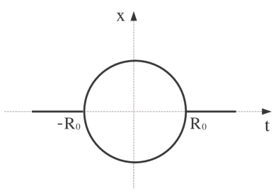
Figure 2: Creation of maximally symmetric Universe.

It shows an ever existing massive point particle that explodes at $t=-R_{0}$, expands to its maximum at $t=0$, and then shrinks back to a point at $t=R_{0}$. This solution is fully compatible with the bulk conservation equation (1). An important conclusion is that the bulk conservation equations do not allow fully bounded braneworld cosmologies. As typical bulk matter respects conventional conservation laws, a typical braneworld can not be created out of nothing.

• Typical braneworld concept does not support Big Bang cosmologies.

To be more precise, the above statement holds in geodesically complete bulks of trivial topology, irrespectively of the bulk signature.

VI Recapitulation

The purpose of this work has been to demonstrate how a stable conventional Universe emerges from a brane embedded in Euclidean bulk. To this end, I had to solve two major problems. First, the stability of the brane dynamics is ensured by employing Euclidean, rather than Minkowskian bulk. Second, I demonstrated how a particular geometry of Euclidean signature can effectively be seen as Minkowskian. To achieve this, I have examined the behavior of a $3$-brane in a $5$-dimensional Euclidean bulk. No bulk action was initially specified. Instead, the brane equations are derived from the universally valid conservation equations of the bulk stres tensor. Specifically, I have investigated small perturbations of the $3$-sphere. The corresponding world-sheet is interpreted as the Universe.

The obtained results are summarized as follows. First, the equation of state $p=\alpha\rho$ for maximally symmetric $3$-branes has been shown to have a universal character in the sector of small $\rho$. This way, the general form of the unperturbed brane equations has been derived, irrespectively of the nature of the brane constituent matter. Second, the stability analysis has lead me to the constraint $\alpha<0$, as a necessary condition for the stable brane world-sheet in Euclidean bulk. The corresponding perturbation equation turns out to have a Klein-Gordon-like kinetic term, based on the auxiliary metric of Minkowski signature. It has been argued that it is this auxiliary metric that is detected in physical measurements. Indeed, the spacetime geometry is always probed by some kind of test matter. In our case, the observed matter stems from the brane vibrations. As these are guided by a Klein-Gordon-like equation, their detection reveals the above mentioned auxiliary metric as a physical metric of the Universe. The third result concerns the effective Universe thus obtained. Its unperturbed evolution has been rewritten in the conventional GR form, and compared with the standard cosmology. The present epoch values of the average energy density and pressure are calculated along with the effective cosmological constant and the age of the Universe. Unfortunately, the more complex issues, such as creation of structure or the origin of anisotropies, cannot be addressed in this simple model. Indeed, the very inclusion of matter requires a bulk of dimension $D\gg 5$. Finally, I have demonstrated that braneworld concept rules out the Big Bang cosmology. This is a consequence of the assumed bulk conservation equations, which are incompatible with the creation out of nothing.

At the end, let me explain the philosophy that lies behind the main achievement of this paper. Basically, it is the idea to obtain the observable physics as a physics of brane vibrations. This is a kind of geometrization program which is not easy to achieve. The main obstacle stems from the fact that brane constituent matter has its own dynamics. To construct a plausible theory of brane vibrations, one should find a mechanism to suppress internal brane dynamics. The problem is similar to the problem of unobservable extra dimensions in Kaluza-Klein theories. There, the extreme smallness of the internal space solves the problem. In the braneworld approach, one could require an extreme brane tension. The search for a bulk Lagrangian that supports a high tension brane is a difficult task, which will be addressed elsewhere.

- (1) L. Randall and R. Sundrum, Phys. Rev. Lett. 83, 3370 (1999).
- (2) L. Randall and R. Sundrum, Phys. Rev. Lett. 83, 4690 (1999).
- (3) T. Regge and C. Teitelboim, in Proceedings of the Marcel Grossman Meeting, Trieste, Italy, 1975, edited by R. Ruffini (North-Holland, Amsterdam, 1977), p.77.
- (4) A. Davidson and D. Karasik, Mod. Phys. Lett. A 13, 2187 (1998).
- (5) A. Davidson and D. Karasik, Phys. Rev. D 67, 064012 (2003).
- (6) R. Cordero, M. Cruz, A. Molgado and E. Rojas, Class. Quant. Grav. 29, 175010 (2012).
- (7) V. A. Rubakov and M. E. Shaposhnikov, Phys. Lett. B 125, 136 (1983).
- (8) M. Visser, Phys. Lett. B 159, 22 (1985).
- (9) E. J. Squires, Phys. Lett. B 167, 286 (1986).
- (10) M. Gogberashvili, Europhys. Lett. 49, 396 (2000).
- (11) A. Boyarsky, A. Neronov and I. Tkachev, Phys. Rev. Lett. 95, 091301 (2005).
- (12) M. Vasilić and M. Vojinović, Phys. Rev. D 73, 124013 (2006).
- (13) M. Vasilić and M. Vojinović, J. High Energy Phys. 07, 028 (2007).
- (14) M. Mathisson, Acta. Phys. Pol. 6, 163 (1937).
- (15) A. Papapetrou, Proc. R. Soc. A 209, 248 (1951).
- (16) B. Santos, J. C. Carvalho and J. S. Alcaniz, Astropart. Phys. 35, 17 (2011).