A Comparison Between Global Proxies of the Sun’s Magnetic Activity Cycle: Inferences from Helioseismology

1 Introduction

section[introduction] The last solar activity cycle (Cycle 23) was unusual in that it was abnormally long ($>12\,\rm years$), and the minimum that followed it was noticeably deeper than any observed since the early 1900s. Recent work by Livingston, Penn, and co-authors, using infrared measurements, suggest that the maximum magnetic-field strength in sunspots has weakened since around 1998 (Livingston, 2002; Penn and Livingston, 2006, 2011; Livingston, Penn, and Svalgaard, 2012; Watson, Penn, and Livingston, 2014). These results, however, remain controversial, with other studies showing that the most dominant observed trends are simply those associated with the regular solar-cycle variation (Watson, Fletcher, and Marshall, 2011; Pevtsov et al., 2011; Rezaei, Beck, and Schmidt, 2012; Pevtsov et al., 2014). Nagovitsyn, Pevtsov, and Livingston (2012) found that a long-term decline in the sunspot field strength was observed when both large and small sunspots were included in the data but that only solar-cycle variations were present when only sunspots with the strongest magnetic fields were included. Nagovitsyn, Pevtsov, and Livingston (2012) explain this in terms of a change in the fraction of large and small sunspots.

Inspired by this controversy, comparisons have been made between sunspot number (SSN) variation, which is a measure of the number of spots on the visible solar disk, and other global proxies of the Sun’s magnetic field, such as the 10.7cm radio flux (F_10.7). Many of these comparisons show that proxies that were in good agreement with each other in previous solar cycles (before Solar Cycle 23) are now diverging (Livingston, Penn, and Svalgaard, 2012; Clette and Lefèvre, 2012). It is now well-known that biases exist in the sunspot-number statistics (see Clette et al., 2014 for a recent review). Although corrections to the sunspot-number trend do reduce some of the observed deviations between the SSN and F_10.7, significant departures persist after 2002, implying that the discrepancy indicates a true change on the Sun (Lefèvre and Clette, 2011; Clette et al., 2014).

Clette et al. (2014) also observed a decline in the ratio of the observed SSN and a synthetic SSN constructed from the Mount Wilson Observatory Magnetic Plage Strength Index: Solar- cycle variations were visible in the ratio but there was also an underlying systematic decline over the past two solar cycles. Furthermore, Clette et al. (2014) also demonstrated a decrease in the average number of spots per sunspot group in Cycles 23 and 24, which is consistent with the results of Tlatov (2013). Javaraiah (2011) observed a significant change in the growth and decay rates of sunspot groups since the beginning of Cycle 23. These results are consistent with a number of results that demonstrate a deficit in the number of small spots observed at the maximum of Cycle 23 compared to Cycle 22 (Kilcik et al., 2011; Lefèvre and Clette, 2011; Clette and Lefèvre, 2012), since small sunspots are known to be relatively short-lived. However, we note that Nagovitsyn, Pevtsov, and Livingston (2012) observed an increase in the number of small sunspots and a decrease in the number of large sunspots since around 2006.

The solar surface and overlying atmosphere are not the only places where a change in behaviour has been observed. The solar interior also appears to be behaving differently in recent years given expectations based on previous observations. Helioseismology allows the interior of the Sun to be probed by observing the properties of the Sun’s natural acoustic oscillations ($p$-modes). Each oscillation is trapped within a well-defined region of the solar interior, known as a cavity. Solar $p$-modes are sensitive to conditions in these cavities, and as such are affected by the presence of flows and magnetic fields (e.g. Woodard and Noyes, 1985; Palle, Regulo, and Roca Cortes, 1989; Elsworth et al., 1990). One such flow is the meridional circulation, which transports near-surface material poleward and is a key component of many solar-dynamo theories. The meridional -flow speed measured in the last solar minimum (between Cycles 23 and 24) was larger than the flow speed observed in the minimum between Cycles 22 and 23 (Basu and Antia, 2010; Hathaway and Rightmire, 2010). Another well-known flow associated with the solar interior is the torsional oscillation, which is also behaving differently than in the same phase of the previous cycle: The poleward branch of the torsional oscillation that will eventually be associated with Cycle 25 is weaker than expected, given the observations of the previous cycle (Howe et al., 2013). Basu et al. (2012) demonstrated that the low-frequency low-degree [$\ell$] $p$-modes showed almost no solar-cycle associated change in frequency in Cycle 23, despite showing a noticeable variation in Cycle 22. Basu et al. explained this in terms of a thinning of the near-surface “magnetic layer” in Cycle 23, which is believed to be responsible for the observed perturbations in frequency with solar cycle. More recently, Salabert, Garcia, and Turck-Chieze (2015) demonstrated that the frequencies of high-frequency modes varied by 30% less in the rising phase of Cycle 24 than in Cycle 23, which is in agreement with surface and atmospheric measures of the Sun’s magnetic field. However, the frequencies of the low-frequency modes appear to change by the same amount in Cycle 23 and the rising phase of Cycle 24, implying that below 1400 km the magnetic field has not changed.

Basu et al. (2012) also showed that at higher frequencies $(\geq 2450\,\rm\mu Hz)$ the frequencies of the low-$\ell$ $p$-modes behaved in a similar manner in Cycles 22, 23, and the rising phase of Cycle 24. As such, the frequencies of these oscillations can be considered as proxies of the Sun’s magnetic-activity cycle. We define the helioseismic frequency shift as the mean change in frequency with time. The method by which this frequency shift is determined will be described in Section section[heliodata]. Such a helioseismic proxy would be sensitive to the effect of a magnetic field on the solar interior, although it is primarily the influence of the magnetic field in near-surface regions that affects the $p$-mode oscillations (e.g. Libbrecht and Woodard, 1990). If we consider the helioseismic frequency shifts to be a global proxy of the Sun’s magnetic field, it is only natural to compare the helioseismic frequency shifts to other commonly used global proxies of the Sun’s magnetic activity. The observed frequency shifts can be explained in terms of direct (the Lorentz force) and indirect effects (changes in the properties of the cavities). To date there is no agreement as to the exact balance of these two effects (e.g. Roberts and Campbell, 1986; Jain and Roberts, 1994; Dziembowski and Goode, 2005). Comparisons with other activity proxies may help to constrain the nature of the observed frequency shifts.

Comparisons between the activity proxies have been performed previously (e.g. Jimenez-Reyes et al., 1998; Antia et al., 2001; Tripathy et al., 2001; Howe, Komm, and Hill, 2002; Chaplin et al., 2004; Chaplin et al., 2007; Jain, Tripathy, and Hill, 2009; Jain et al., 2012). Chaplin et al. (2007) compared six different proxies with the Sun-as-a-star frequency shifts and demonstrated that better correlations are observed with proxies that measure both the strong and the weak components of the Sun’s magnetic field, such as the 10.7 cm radio flux (as opposed the the sunspot number, which mainly samples the strong magnetic flux). The weak component of the solar magnetic flux is distributed over a wider range of latitudes than the strong component and so a possible explanation of these results is in terms of the latitudinal distribution of the modes used in this study (i.e. low-degree modes). Howe, Komm, and Hill (2002) showed that it is possible to use latitudinal inversion techniques to localize the frequency shifts in latitude and, in fact, reconstruct the evolution of the surface magnetic field. However, this requires spatially resolved data, such as those obtained by the Global Oscillation Network Group (GONG), which has only been collecting data since 1995. The extended solar minimum between Cycles 23 and 24 means that, to date, this only covers approximately one-and-a-half activity cycles, and so cycle-to-cycle comparisons are not yet possible.

We will compare the relationships between the proxies and the helioseismic frequencies observed during the entirety of Cycles 22 and 23, and in the rising phase of Cycle 24. Like Chaplin et al. (2007), we compare the helioseismic frequencies to the sunspot number and 10.7 cm flux. However, we also consider sunspot-area data and the coronal index. Furthermore, we consider two interplanetary proxies of magnetic field (the interplanetary magnetic field and the galactic cosmic-ray flux). We use Birmingham Solar Oscillations Network (BiSON: Chaplin et al., 1996) data, which has been concatenated using new, improved procedures that are described by Davies et al. (2014). We will perform a comparison between the quasi-biennial oscillation (QBO), which is known to exist in the helioseismic frequencies (Broomhall et al., 2009), and the solar and interplanetary proxies (Bazilevskaya et al., 2014). A dedicated comparison between the features of the QBO observed in helioseismic data and those observed in such a wide range of activity proxies has never before been performed.

The remainder of this article is structured as follows: Section section[data] describes the data used in the article. We describe the helioseismic data and the method by which the frequency shifts are obtained (Section section[heliodata]). We also describe the other global proxies considered in this article (Section section[proxydata]). Section section[comparison] describes the comparison of the global proxies with the helioseismic data. We initially consider the differences observed from one 11-year solar cycle to the next. However, we go on to consider shorter-term variations in the solar magnetic field, and the consistency of these variations across the different proxies (Section section[2yr]). Finally, we discuss the implications of these results in Section section[discussion].

2 Data

section[data]

2.1 Helioseismic Data

section[heliodata]

The Birmingham Solar Oscillations Network (BiSON, Chaplin et al., 1996; Davies et al., 2014) consists of six sites that make line-of-sight velocity observations of the Sun. BiSON makes unresolved, Sun-as-a-star observations and so are only sensitive to low-$\ell$ $p$-modes. However, these are the oscillations that sample deep layers of the solar interior. The earliest data observed by individual sites are sporadic and so will not be used here. Nevertheless, BiSON has now been observing the Sun continuously for over 30 years, making it the longest helioseismic data set (bison.ph.bham.ac.uk/) available and consequently ideal for studies of more than one solar cycle. The period 1 January 1985 to 26 March 2014 will be considered, which covers approximately two-and-a-half solar cycles.

When using helioseismic data to study the solar cycle, a balance must be made concerning the length of time series considered. One must use time series that provide enough resolution in the frequency domain to accurately and precisely obtain the frequencies of the oscillations. However, one must also use time series short enough to be able to study the evolution of helioseismic parameters in time. In order to study variations associated with the 11-year cycle we have used 114 consecutive time series of 365-days length that are separated by 91.25 days. However, when considering shorter-term variations we used shorter time series, of length 182.5 days (but still separated by 91.25 days). Although the precision with which we could obtain the frequencies of the oscillations was reduced by this shortening of the time series, this gives a better resolution with which to study variations on timescales less than 11 years. The extracted parameters are essentially the average values observed over the 365-day (or 182.5-day) time period under consideration.

The frequencies of each $p$-mode $[\nu_{l,n}]$ were obtained by fitting an asymmetric profile (Nigam and Kosovichev, 1998) to the frequency power spectra using a maximum-likelihood-estimation technique (Fletcher et al., 2009). Only $p$-modes in the range $2400\leq\nu\leq 3500\,\rm\mu Hz$ were considered here for the following reasons: Firstly, these are the most prominent oscillations meaning their frequencies can be obtained accurately. Secondly, as we move to higher frequencies the lifetimes of the oscillations decrease, meaning they have a wider profile in the power spectrum from which the frequencies are obtained. As a result, the precision with which we can obtain the frequencies of the oscillations decreases with increasing frequency. Finally, this range includes eight overtones of each degree under consideration i.e. there are eight $\ell=0$ modes, eight $\ell=1$ modes, and eight $\ell=2$ modes in this frequency range. Only modes with $0\leq\ell\leq 2$ were considered: The BiSON data have no spatial resolution and so the amplitudes of the modes in the power spectrum with $l\geq 3$ are low, making it hard to determine the frequencies of modes accurately and precisely.We note that the early BiSON data (before approximately 1993) have a relatively low duty cycle as the full BiSON network was not established. Furthermore, because of improvements to the instruments over time, the more recent data are of better quality. This is reflected in the uncertainties associated with the frequencies. In order to compensate for the low duty cycle, when obtaining the mode frequencies, the window function of the data was convolved with the model fitted to the power spectrum (Fletcher et al., 2009). As we only consider the most prominent modes in the frequency spectrum they stll have significant signal-to-noise in the early data. Nevertheless, each fitted function was checked by eye to ensure the frequencies obtained were robust.

Once the frequencies were obtained for each of the 365 day (or 182.5 day) time series an average set of reference frequencies $[\overline{\nu_{n,l}}]$ was determined. This reference set gives the weighted average frequencies observed across the entire 30-year epoch under consideration, where the weights were determined by the uncertainties given by the maximum likelihood fit to the power spectrum. We note that, while the exact choice of time series from which the reference set is constructed can affect the absolute value of frequency shift, the conclusions of this article are not dependent on it. Here, the reference set includes time series obtained when the duty cycle of the data was low and the quality of the observations poorer. However, excluding these from the reference set by, for example, only considering data observed during Cycles 23 and 24, alters the subsequently determined frequency shift by less than $0.5\sigma$. Furthermore, this change is partially explained by a systematic offset caused simply by considering a different time span, and, therefore, a different range of magnetic-activity levels. In real terms, the influence of including the early data is, therefore, negligible.

The frequency shift of an individual mode, in any single 365 day (or 182.5 day) timeseries $[\delta\nu_{n,l,i}$, where $i$ denotes the timeseries under consideration] is then determined by subtracting the relevant reference frequency from the frequency observed in that individual time series, i.e.

$$\ilabel{equation[shift]}\delta\nu_{n,\ell,i}=\nu_{n,\ell,i}-\overline{\nu_{n,\ell}}.$$ (1)

We then determine the weighted-average frequency shift $[\overline{\delta\nu_{i}}]$ for all modes with $0\leq\ell\leq 2$ and $2400\leq\nu\leq 3500\,\rm\mu Hz$. Each frequency shift has an associated uncertainty $[\sigma_{i}]$. We compared these frequency shifts to other well-known proxies of the solar magnetic field, which we now describe.

2.2 Global Proxy Data

section[proxydata]

Perhaps the best-known global-activity proxy is the sunspot number (SSN), which is a measure of the number of sunspot groups and individual sunspots on the solar surface. Here we use the NOAA International Sunspot Number (www.ngdc.noaa.gov: see discussion by Clette et al., 2014). Although historically important because of its longevity, the SSN has occasionally been criticised for its lack of physicality. Therefore we also consider sunspot area (solarscience.msfc.nasa.gov/greenwch.shtml: SA: Hathaway, 2010), as an alternative measure of the photospheric magnetic flux. The 10.7cm radio flux (www.ngdc.noaa.gov: F_10.7) is a proxy for the solar activity in the upper chromosphere and lower corona, and is sensitive to both strong and weak magnetic-field regions (Tapping, 1987). F_10.7 is expressed in Radio Flux Units [RFU: $\rm 1\,RFU=10^{-22}\,W\,m^{-2}\,Hz^{-1}$]. The coronal index (www.ngdc.noaa.gov: CI: Mavromichalaki et al., 2005) is a measure of the total power emitted by the green corona at 530.3 nm, which corresponds to the Fe xiv spectral line. The above proxies are observe at different levels in the solar atmosphere because they are sensitive to different temperatures, and therefore, indirectly, the magnetic-field strength. Consequently, they can be considered as proxies of the solar magnetic field in some region of the solar atmosphere. In the remainder of the article we refer to these four proxies as solar proxies. We also compare the helioseismic data with two more remote measures of the Sun’s magnetic field, which we refer to as interplanetary proxies. We consider the interplanetary magnetic field (IMF) as extracted from NASA/GSFC’s OMNI data set through OMNIWeb (omniweb.gsfc.nasa.gov: King and Papitashvili, 2005). We also consider the galactic cosmic-ray intensity (CR) obtained from the Moscow neutron monitor (cosrays.izmiran.ru/main.htm: Bazilevskaya et al., 2013). Averages of all of the proxies were taken over the same 365-day (or 182.5-day) time periods from which the helioseismic frequencies were determined.

3 Comparison of Global Proxies of the Sun’s Magnetic Activity Cycle with Helioseismic Frequency Variations

section[comparison]

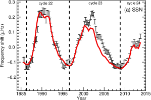
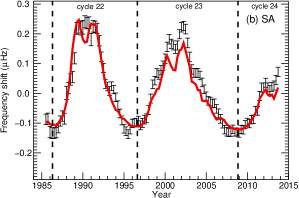
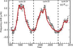
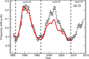
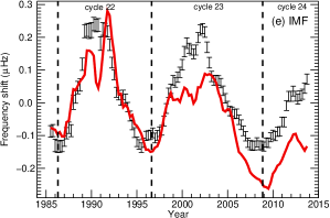
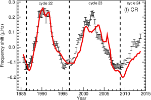
Figure 1.: Averaged frequency shifts of helioseismic modes (data with plotted uncertainties) obtained using $0\leq\ell\leq 2$ and $2400\leq\nu\leq 3500\,\rm\mu Hz$. The results were obtained from 365-day BiSON time series, which are separated by 91.25 days. Red, solid lines represent linearly regressed versions of other activity proxies and the coefficients of the linear regressions can be found in Table table[fits]. Since CR varies in antiphase with solar cycle the gradient of the linear regression for CR (panel f) is negative. Panel a: Scaled sunspot number. Panel b: Scaled sunspot area. Panel c: Scaled 10.7 cm radio flux. Panel d: Scaled coronal index. Panel e: Scaled interplanetary magnetic field. Panel f: Inversely scaled galactic cosmic ray intensity. The vertical dashed lines separate different solar cycles.figure[shifts˙time]

Figure figure[shifts_time] plots the average $p$-mode frequency shifts $[\overline{\delta\nu_{i}}]$ as a function of time. The amplitudes of the minimum-to-maximum variation of the proxies (including the helioseismic frequency shifts) are very different. For example, an $\ell=0$ mode with a frequency of $3000\,\rm\mu Hz$ experiences a shift in frequency of approximately $0.4\,\rm\mu Hz$ between solar minimum and maximum, whereas the sunspot number changes by over 100 and the sunspot area increases by of the order of 2000 millionths of a solar hemisphere (msh). Furthermore, CR varies in antiphase with solar cycle, such that the intensity is at a maximum at solar minimum. To allow a comparison of the frequency shifts with the proxies a linear regression between the global proxies and the frequency shifts was performed. Only values observed during Cycle 22 (between 1 January 1985 and 29 December 1996) were used in the regression. This time span includes data from when the duty cycle was relatively low and thus the quality relatively poor in comparison to more recent observations. However, the aim of this paper is to determine whether the relationship between proxy and helioseismic frequency shift varies from one cycle to the next. In this respect the conclusions of this article would not be altered by scaling with respect to a different cycle: One could scale with respect to Cycle 23 and determine the degree of divergence observed in Cycle 22.

The coefficients for the linear regressions can be found in Table table[fits]. Since the data are overlapping, Monte Carlo simulations were used to determine the uncertainties associated with the linear regressions. These simulations added randomly-generated, Gaussian-distributed noise to the frequency shifts, where the standard deviation of the random numbers were based on the associated uncertainties. The randomly-generated noise accounted for the fact that the uncertainties of adjacent points ($i$ and $i+1$ say) have a 75% correlation and that this decreases to 50% at $i+2$, 25% at $i+3$, and is zero at $i+4$. This linear regression has been used to scale the global proxies and these scaled proxies are also plotted as a function of time in Figure figure[shifts_time]. Note that CR is inversely scaled, and that the inversely scaled CR varies in phase with the other proxies. The scaled proxy values $[\delta\nu_{\textrm{\scriptsize{p}}}]$ observed during Cycles 23 and 24 can be regarded as retrospective predictions of the frequency shifts we would expect to observe given the relationship between the proxies and the frequency shifts observed during Cycle 22.

Table 1.: Coefficients of linear regressions between helioseismic-frequency shifts and global proxies for the two complete solar cycles under consideration. The units in which the gradient of the linear regression is measured depend on the proxy under consideration. We have used proxy unit (PU) as a global proxy unit where PU is equivalent to msh for SA; RFU for F_10.7; $\rm W\,sr^{-1}$ for CI; nT for IMF; impacts min^-1 for CR.We recall that SSN is a number with no units. table[fits]

Proxy	Cycle	Gradient	Intercept	Reduced	Gradient	Intercept
		$\times 10^{-3}$		$\chi^{2}$	Difference	Difference
		$[\mu\rm Hz\,PU^{-1}]$	$[\rm\mu Hz]$		$[\sigma]$	$[\sigma]$
SSN	22	$2.39\pm 0.10$	$-0.145\pm 0.008$	3.16	$2.0$	$2.0$
	23	$2.67\pm 0.10$	$-0.124\pm 0.007$	4.74
SA	22	$0.144\pm 0.006$	$-0.123\pm 0.007$	3.83	$4.0$	$0.2$
	23	$0.181\pm 0.007$	$-0.125\pm 0.006$	1.80
F10.7	22	$2.51\pm 0.10$	$-0.293\pm 0.013$	2.73	$0.9$	$0.1$
	23	$2.64\pm 0.10$	$-0.291\pm 0.012$	2.89
CI	22	$24.3\pm 1.0$	$-0.181\pm 0.009$	3.55	$7.4$	$1.5$
	23	$36.4\pm 1.3$	$-0.200\pm 0.009$	3.01
IMF	22	$91.7\pm 3.9$	$-0.620\pm 0.022$	12.69	$0.7$	$2.9$
	23	$88.2\pm 3.6$	$-0.529\pm 0.022$	12.03
CR	22	$-0.239\pm 0.010$	$2.11\pm 0.08$	3.00	$1.7$	$1.6$
	23	$-0.216\pm 0.009$	$1.93\pm 0.08$	14.76

We first consider the SSN. Up until around 2000, the agreement is good but in the declining phase of Cycle 23 discrepancies emerge, although the agreement does appear to improve again in Cycle 24. The helioseismic frequency shifts are more compatible with the sunspot area and F_10.7 predictions, both of which show reasonably good agreement with the helioseismic frequencies throughout. As we move farther out in the Sun’s atmosphere by considering the coronal index we can see that the predicted values differ substantially from the observed frequency shifts during Cycle 23: The agreement is poor for the majority of Cycle 23. Unfortunately measurements of the coronal index ceased in 2008 and so we cannot make this comparison in Cycle 24. However, this highlights the need to maintain long-duration observations of the Sun at multiple wavelengths. Similarly large departures between the observed frequency shifts and the frequency shifts predicted by the IMF are observed in Cycles 23 and 24. However, we note that, for the IMF, the agreement between the observed and predicted frequency shifts during Cycle 22 is poor in comparison with the other proxies. Although the helioseismic-frequency shifts and the cosmic-ray predictions (based on the inverse scaling) are more consistent than the IMF, significant departures remain in both Cycles 23 and 24.

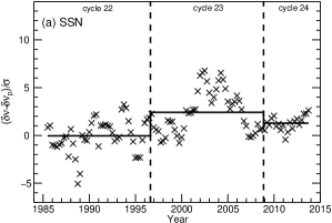
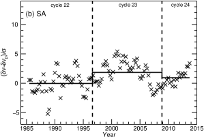
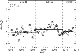
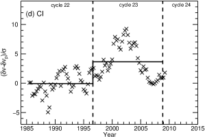
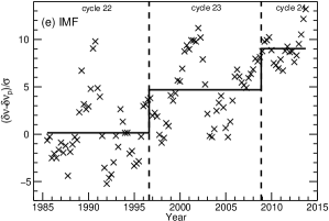
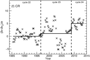
Figure 2.: Scaled residuals $[(\delta\nu_{i}-\delta\nu_{\textrm{\scriptsize{p,}}i})/\sigma]$ as a function of time, where $\delta\nu_{i}$ is the observed helioseismic-frequency shift, $\sigma_{i}$ is the uncertainty associated with this frequency shift, and $\delta\nu_{\textrm{\scriptsize{p,}}i}$ is the frequency shift predicted by the linear regression for each proxy. The linear regressions were performed using data from Cycle 22 only and the values can be found in Table table[fits]. The average values for each cycle are plotted as horizontal solid lines in black. Panel a: sunspot number. Panel b: sunspot area. Panel c: 10.7 cm radio flux. Panel d: coronal index. Panel e: interplanetary magnetic field. Panel f: galactic cosmic-ray intensity. figure[residuals]

To assess the significance of these variations we determined the difference between the observed and predicted frequency shifts $[\delta\nu_{i}-\delta\nu_{\textrm{\scriptsize{p,}}i}]$ and then divided by the uncertainty associated with the frequency shifts $[\sigma_{i}]$. This uncertainty is derived from the uncertainty obtained from fitting the frequency power spectrum (described in Section section[heliodata]). These results are plotted in Figure figure[residuals]. For convenience, the average ratio observed during each activity cycle is plotted. We remind the reader that the proxies were scaled with respect to the values observed in Cycle 22, it is therefore expected that the average ratio in Cycle 22 is approximately zero. For all proxies the agreement between the observed and predicted frequency shifts is worse during Cycle 23 than Cycle 22. We note here that that does not necessarily mean that the agreement between the absolute values of the proxies and the helioseismic frequencies is worse as we must remember that we have used the relationship observed between the proxies and the frequencies in Cycle 22 to make the prediction. However, this figure does imply that the relationship between the proxies and the frequency shifts changes from Cycle 22 to Cycle 23. On average the ratios are positive in Cycle 23, meaning that the predictions underestimate the shift in frequency. Furthermore, there are systematic trends in the ratios plotted in Figure figure[residuals], with the ratios being largest at solar maximum. This all implies that the linear regression is steeper in Cycle 23 than was observed in Cycle 22. This is supported by the results of Table table[fits], which shows that, for the solar proxies, the gradient of the linear regression is steeper in Cycle 23 than Cycle 22. We also note that the difference in the gradient is significant for SA and CI. Interestingly for the interplanetary proxies the gradient of the linear regression is steeper in Cycle 22 than Cycle 23. We remind the reader that CR is inversely scaled and so the gradient has a larger negative value in Cycle 22 than Cycle 23. Although on first inspection this seems contradictory to the result plotted in Figure figure[shifts_time] it can be explained in terms of a change in the intercept (which acts as an offset). In particular this would produce better agreement between the proxies and the frequency shifts in the minimum between Cycles 23 and 24 when large discrepancies are observed for the interplanetary proxies. We also note here that the reduced $\chi^{2}$ of the linear regressions of the interplanetary proxies is larger than for the solar proxies (with the exception of CR in Cycle 22, see Table table[fits]).

The ratios plotted in Figure figure[residuals] decrease in Cycle 24 compared to Cycle 23 for SSN, SA, and F_10.7, implying that the relationship between these proxies and the frequency shifts is returning to something similar to that observed in Cycle 22. On the other hand the ratios increase further for the interplanetary proxies (IMF and CR).

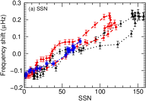
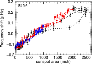
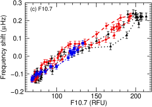
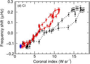
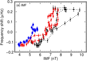
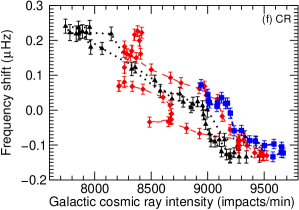
Figure 3.: Frequency shifts as a function of the global proxies. The different colours represent the different cycles: the black-dotted line with triangle symbols represents Cycle 22, the red-dashed line with diamond symbols represents Cycle 23 and the blue-triple-dot-dashed line with square symbols represents Cycle 24. Panel a: sunspot number. Panel b: sunspot area. Panel c: 10.7 cm radio flux. Panel d: coronal index. Panel e: interplanetary magnetic field. Panel f: galactic cosmic-ray intensity.figure[shifts˙vs˙proxies]

Figure figure[shifts_vs_proxies] shows the frequency shifts plotted directly as a function of the unscaled global activity proxies. Since Figure figure[shifts_vs_proxies] plots the unscaled activity proxies there is no reliance on the linear regression. However, Figure figure[shifts_vs_proxies] still clearly shows that the relationship between the activity proxies and the helioseismic-frequency shifts varies from one cycle to the next. Notice that the relationship between the frequency shifts and the proxies is only approximately linear. The well-known hysteresis is also observed (e.g. Jimenez-Reyes et al., 1998; Tripathy et al., 2000; Chaplin et al., 2007; Jain, Tripathy, and Hill, 2009). This occurs because of the distribution in latitude of the surface magnetic flux: Sunspots are known to appear at mid-latitudes and migrate towards the Equator as the cycle progresses. Some $p$-modes are more sensitive to low-latitude regions than others (depending on the harmonic degree $[\ell]$ and azimuthal degree $[m]$ that describe the spherical harmonic of the mode) and so as the cycle evolves and the Sun’s magnetic field migrates towards the Equator the influence of the Sun’s magnetic field on each mode varies (Moreno-Insertis and Solanki, 2000). We note here that comparisons between solar-cycle associated frequency shifts and the appropriate spherical-harmonic decomposition of the surface magnetic flux result in a good linear relationship (e.g. Howe, Komm, and Hill, 1999; Howe, Komm, and Hill, 2002).

To assess the significance of the hysteresis, we performed separate linear regressions for the rising and falling phases of each cycle and the coefficients can be found in Table table[fits_rise_fall]. A comparison of the gradients of the rising and falling phases in any one cycle is very dependent on which proxy is considered and which cycle. For example, for any one cycle, the gradient of the linear regression obtained with the sunspot-area data is similar in the rising and falling phases, indicating a minimal amount of hysteresis. This is particularly true for Cycle 23. On the other hand SSN, F_10.7, CI, and CR all show an increase in hysteresis in Cycle 23 compared with Cycle 22. The IMF shows a decrease in hysteresis in Cycle 23. We also note that the IMF is the only proxy for which the gradient is steeper in the rising phase of the cycle than the falling phase. However, we note from Figure figure[shifts_vs_proxies], and from the large reduced $\chi^{2}$-values obtained that a linear relationship is not really appropriate.

Table 2.: Linear fits between helioseismic-frequency shifts and global proxies for rising and falling phases of the solar cycle. The units in which the gradient of the linear regression is measured depends on the proxy under consideration. We have used proxy unit (PU) as a global proxy unit where PU is equivalent to msh for SA; RFU for F_10.7; $\rm W\,sr^{-1}$ for CI; nT for IMF; impacts min^-1 for CR. We recall that SSN is a number with no units.table[fits˙rise˙fall]

Proxy	Cycle	Rising			Falling			Difference
		Gradient	Intercept	Reduced	Gradient	Intercept	Reduced	Gradient	Intercept
		$(\times 10^{-3})$		$\chi^{2}$	$(\times 10^{-3})$		$\chi^{2}$
		$[\rm\mu Hz\,PU^{-1}]$	$[\rm\mu Hz]$		$[\rm\mu Hz\,PU^{-1}]$	$[\rm\mu Hz]$		$\sigma$	$\sigma$
SSN	22	$2.28\pm 0.14$	$-0.154\pm 0.012$	2.71	$2.51\pm 0.12$	$-0.143\pm 0.009$	2.63	$1.2$	$0.7$
	23	$2.52\pm 0.16$	$-0.140\pm 0.013$	1.42	$3.09\pm 0.14$	$-0.126\pm 0.008$	2.31	$2.7$	$0.9$
	24	$2.53\pm 0.23$	$-0.131\pm 0.010$	0.575
SA	22	$0.139\pm 0.008$	$-0.132\pm 0.011$	4.10	$0.148\pm 0.007$	$-0.119\pm 0.009$	3.32	$0.8$	$0.9$
	23	$0.178\pm 0.012$	$-0.120\pm 0.012$	2.14	$0.182\pm 0.008$	$-0.127\pm 0.008$	1.76	$0.3$	$0.5$
	24	$0.181\pm 0.017$	$-0.128\pm 0.010$	0.707
F10.7	22	$2.46\pm 0.15$	$-0.298\pm 0.019$	2.89	$2.55\pm 0.13$	$-0.292\pm 0.015$	1.20	$0.5$	$0.2$
	23	$2.52\pm 0.16$	$-0.287\pm 0.022$	1.20	$2.81\pm 0.12$	$-0.302\pm 0.014$	3.14	$1.5$	$0.6$
	24	$2.87\pm 0.26$	$-0.324\pm 0.265$	0.505
CI	22	$23.6\pm 1.4$	$-0.200\pm 0.014$	2.27	$25.5\pm 1.2$	$-0.176\pm 0.011$	2.39	$1.0$	$1.3$
	23	$33.9\pm 2.2$	$-0.192\pm 0.016$	2.82	$38.7\pm 1.7$	$-0.207\pm 0.011$	2.65	$1.7$	$0.8$
IMF	22	$128.6\pm 7.7$	$-0.870\pm 0.052$	4.23	$80.1\pm 4.4$	$-0.540\pm 0.030$	16.33	$5.5$	$5.5$
	23	$125.7\pm 8.8$	$-0.780\pm 0.057$	11.27	$82.9\pm 4.0$	$-0.493\pm 0.024$	11.27	$4.4$	$4.6$
	24	$100.2\pm 9.9$	$-0.530\pm 0.049$	3.62
CR	22	$-0.228\pm 0.013$	$2.02\pm 0.12$	2.68	$-0.249\pm 0.012$	$2.20\pm 0.11$	3.11	$1.2$	$1.1$
	23	$-0.247\pm 0.017$	$2.28\pm 0.15$	4.35	$-0.209\pm 0.011$	$1.84\pm 0.09$	17.98	$1.9$	$2.5$
	24	$-0.258\pm 0.024$	$2.36\pm 0.23$	2.10

3.1 Short-term Variation

section[2yr]

It is well known that short term ($\approx$two-year) variations exist on top of the 11-year cycle in both the helioseismic-frequency shifts and other proxies of the solar activity (see Bazilevskaya et al., 2014 for a recent review). Such variations are often referred to as a quasi-biennial oscillation (QBO). These variations can be seen in Figure figure[shifts_time] but can be viewed more clearly once the 11-year cycle is removed. A smoothed version of the frequency shifts was subtracted from the raw frequency shifts (plotted in Figure figure[shifts_time]), where the smoothing was performed over three years. At the edges additional end points based on the values of the first and last values respectively were used to artificially extend the array and allow the smoothing to be completed. The residuals are plotted in Figure figure[QBO]. Once again a scaled version of the proxies is plotted for comparison (note again that CR is inversely scaled). To maintain consistency, the linear regressions were performed using the raw proxies and frequency shifts, not the residuals. In Figure figure[QBO] the short-term variations are clear in both the frequency shifts and the proxies, especially around solar maximum. An enhanced amplitude around solar maximum is a well-known property of the QBO (see Bazilevskaya et al., 2014 and references therein). Note that the amplitude of the QBO is consistent between the proxies and the frequency shifts despite the fact that the raw values, which are dominated by the 11-year cycle, were used to scale the proxies.

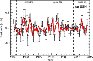
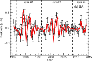
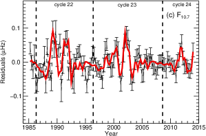
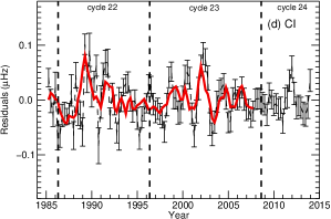
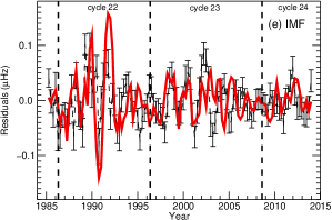
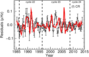
Figure 4.: Frequency-shift residuals as a function of time (black-dashed line). The residuals are determined by subtracting three-year-smoothed frequency shifts from the frequency shifts plotted in Figure figure[shifts_time]. Scaled versions of the activity proxies are plotted in coloured, solid lines. The activity proxies were scaled with respect to the raw proxies and frequency shifts and not the residuals themselves. As with Figure figure[shifts_time] CR was regressed with a negative gradient. Panel a: scaled sunspot number. Panel b: scaled sunspot area. Panel c: scaled 10.7 cm radio flux. Panel d: scaled coronal index. Panel e: scaled interplanetary magnetic field. Panel f: inversely scaled galactic cosmic ray intensity.figure[QBO]

Table table[QBO] shows the correlations of the unscaled proxy residuals with the frequency -shift residuals. We note that the correlations were determined using only independent data points (here those with even subscripts were used). There is a definite split between the solar proxies (SSN, SA, F_10.7, and CI) and the interplanetary proxies (IMF, CR). For the solar proxies, the correlation is higher in Cycle 23 than in Cycle 22. However, the poor correlations observed during Cycle 22 could simply be a reflection of the fact that the helioseismic data were of poorer quality. The situation is different for the interplanetary proxies, where the correlations are lower in Cycle 23 (and Cycle 24) than was observed in Cycle 22. We must remember that we are currently in the maximum phase of Cycle 24, when the amplitude of the quasi-biennial periodicity is at a maximum and so it would be misleading to compare the correlation observed in Cycle 24 with Cycles 22 and 23. However, we note from Figure figure[QBO] and Table table[QBO] that the data are highly correlated with the solar proxies in Cycle 24 thus far. As one might expect, correlations between activity proxies and helioseismic-frequency shifts (not residuals) are higher in the rising and falling phases, where relatively large changes in time are observed, than around solar maxmimum and minimum, where the proxies and helioseismic frequencies are approximately constant (e.g. Jain, Tripathy, and Hill, 2009). The QBO, on the other hand, appears to be most highly correlated around solar maximum, where the amplitude of the QBO is largest.

Table 3.: Correlations between helioseismic-frequency residuals and solar activity proxies. We note that only the rising phase and a part of the maximum of Cycle 24 are analysed.table[QBO]

Proxy	Cycle	Pearson’s		Spearman’s
		$r$	Probability	$r_{s}$	Probability
SSN	all	0.57	$6.1\times 10^{-7}$	0.47	$1.6\times 10^{-4}$
	22	0.45	0.014	0.31	0.15
	23	0.77	$1.8\times 10^{-6}$	0.63	$9.0\times 10^{-4}$
	24	0.90	$7.1\times 10^{-6}$	0.78	0.0030
SA	all	0.47	$8.1\times 10^{-5}$	0.32	0.014
	22	0.37	0.040	0.22	0.32
	23	0.57	0.0015	0.45	0.028
	24	0.90	$4.1\times 10^{-6}$	0.77	0.0034
F10.7	all	0.64	$8.3\times 10^{-9}$	0.50	$6.3\times 10^{-5}$
	22	0.55	0.0028	0.32	0.14
	23	0.76	$2.6\times 10^{-6}$	0.63	$9.6\times 10^{-4}$
	24	0.90	$4.18\times 10^{-6}$	0.76	0.0045
CI	all	0.42	$4.3\times 10^{-4}$	0.34	0.065
	22	0.50	0.0074	0.39	0.065
	23	0.67	$1.3\times 10^{-4}$	0.65	$8.6\times 10^{-4}$
IMF	all	0.52	$7.6\times 10^{-6}$	0.42	$8.6\times 10^{-4}$
	22	0.62	$5.7\times 10^{-4}$	0.59	0.0029
	23	0.30	0.082	0.22	0.31
	24	0.33	0.15	0.54	0.071
CR	all	-0.45	$1.4\times 10^{-4}$	-0.40	0.0016
	22	-0.70	$4.5\times 10^{-5}$	-0.67	$5.2\times 10^{-4}$
	23	-0.12	0.30	-0.12	0.56
	24	-0.11	0.37	-0.12	0.7

4 Discussion

section[discussion] If proven to be true, one of the consequences of the apparent decrease in the average magnetic field of sunspots observed by, for example, Livingston, Penn, and Svalgaard (2012) is that, if the decrease continues, fewer small sunspots will be observed. Penn and Livingston (2006) found that sunspots can only form if the magnetic-field strength exceeds 1500 G. If the magnetic-field strength is weaker, the field penetrating the solar surface is more diffuse rather than clustering in small pores and spots. Not only does this explain the apparent divergence between the 10.7 cm flux (which is sensitive to both strong magnetic field regions and weaker faculae and plages) and the SSN (Livingston, Penn, and Svalgaard, 2012) but it is also consistent with the apparent deficit in the number of small spots observed at the maximum of Cycle 23 compared to Cycle 22 (Kilcik et al., 2011; Lefèvre and Clette, 2011; Clette and Lefèvre, 2012). Sunspot area is dominated by the largest active regions and so is less sensitive to this small-spot deficit than SSN, which gives equal weighting to spots of all sizes and is, therefore, dominated by small spots, which are most abundant. The coronal index, which is connected with the green-line emission produced by ionised iron, is associated with a specific temperature of the plasma. The discrepancies with the other activity proxies show that, while the coronal index may be affected by the sunspot deficit, other features, such as coronal holes, are very important in determining the observed values. For example Abramenko et al. (2010) observed that the area of low-latitude coronal holes increased in the declining phase of Cycle 23.

These results therefore imply that the observed frequency shifts are the result of both strong and weak-magnetic-field regions. Although the size of the frequency shift is dependent on the strength of the magnetic field, a shift of some magnitude will be observed no matter what the strength of the magnetic field is. This is similar to the 10.7 cm flux but in contrast to the SSN, which has a magnetic-field strength threshold, below which no sunspot is formed. It is, therefore, understandable that better agreement is observed between the helioseismic frequencies and the 10.7 cm flux than the SSN. This is in agreement with the results of Chaplin et al. (2007). Given the frequency range under consideration here, our results are also in agreement with Salabert, Garcia, and Turck-Chieze (2015), who found that the variation in the frequencies of high-frequency modes reflects the variation observed in the 10.7 cm radio flux. These results also imply that the additional effects that brought about a reduction in the CI in Cycle 23 (such as low-latitude coronal holes) are not reliant on the magnetic field in the solar interior. There is also clear evidence for a change in the relationship between the interplanetary proxies and the helioseismic data since Cycle 22.

The differences in the 11-year cycles become even more interesting when we consider the QBO. For the solar proxies, the frequency-shift residuals and the proxy residuals are highly correlated in all cycles, and in particular Cycles 23 and 24. Additionally, there is no divergence in amplitude indicating that, in terms of the QBO, there is no change in relationship between the proxies and the helioseismic-frequency shifts. Conversely the interplanetary-proxy residuals and the helioseismic-frequency-shift residuals are poorly correlated in Cycles 23 and 24. Interestingly, the decoupling of the QBOs appears to have occurred around 2000 (see Figure figure[QBO]). This is approximately the same time that the 11-year cycles in the global proxies began to diverge.

Finally we recall that in Figure figure[residuals], for the solar proxies, the scaled residuals decreased in Cycle 24 compared to Cycle 23. This raises the tantalising question as to whether we are simply observing a 22-year Hale cycle effect, where by the frequency shifts and the proxies display one relationship in even cycles and a different relationship in odd cycles.

Acknowledgments

A.-M. Broomhall thanks the Institute of Advanced Study, University of Warwick for their support. V.M. Nakariakov: This work was supported by the European Research Council under the SeismoSun Research Project No. 321141, STFC consolidated grant ST/L000733/1, and the BK21 plus program through the National Research Foundation funded by the Ministry of Education of Korea. We thank the Birmingham Solar Oscillations Network, IZMIRAN Cosmic Ray Group, NOAA NGDC, OMNIWeb, and the Royal Observatory (Greenwich) for making their data freely available. We acknowledge use of NASA/GSFC’s Space Physics Data Facility’s OMNIWeb (or CDAWeb or ftp) service, and OMNI data. We acknowledge the Leverhulme Trust for funding the “Probing the Sun: inside and out” project upon which this research is based. The research leading to these results has received funding from the European Community’s Seventh Framework Programme ([FP7/2007-2013]) under grant agreement n° 312844 (see Article II.30. of the Grant Agreement).

Disclosure of Potential Conflicts of Interest

The authors declare that they have no conflicts of interest.

References

- Abramenko et al. (2010) Abramenko, V., Yurchyshyn, V., Linker, J., Mikić, Z., Luhmann, J., Lee, C.O.: 2010, Low-Latitude Coronal Holes at the Minimum of the 23rd Solar Cycle. Astrophys J. 712, 813. DOI. ADS.
- Antia et al. (2001) Antia, H.M., Basu, S., Hill, F., Howe, R., Komm, R.W., Schou, J.: 2001, Solar-cycle variation of the sound-speed asphericity from GONG and MDI data 1995-2000. Mon. Not Roy. Astron. Soc. 327, 1029. DOI. ADS.
- Basu and Antia (2010) Basu, S., Antia, H.M.: 2010, Characteristics of Solar Meridional Flows during Solar Cycle 23. Astrophys J. 717, 488. DOI. ADS.
- Basu et al. (2012) Basu, S., Broomhall, A.-M., Chaplin, W.J., Elsworth, Y.: 2012, Thinning of the Sun’s Magnetic Layer: The Peculiar Solar Minimum Could Have Been Predicted. Astrophys J. 758, 43. DOI. ADS.
- Bazilevskaya et al. (2013) Bazilevskaya, G.A., Krainev, M.B., Svirzhevskaya, A.K., Svirzhevsky, N.S.: 2013, Galactic cosmic rays and parameters of the interplanetary medium near solar activity minima. Cosmic Research 51, 29. DOI. ADS.
- Bazilevskaya et al. (2014) Bazilevskaya, G., Broomhall, A.-M., Elsworth, Y., Nakariakov, V.M.: 2014, A Combined Analysis of the Observational Aspects of the Quasi-biennial Oscillation in Solar Magnetic Activity. Space Sci. Rev. 186, 359. DOI. ADS.
- Broomhall et al. (2009) Broomhall, A.-M., Chaplin, W.J., Elsworth, Y., Fletcher, S.T., New, R.: 2009, Is the Current Lack of Solar Activity Only Skin Deep? Astrophys J. Lett. 700, L162. DOI. ADS.
- Chaplin et al. (1996) Chaplin, W.J., Elsworth, Y., Howe, R., Isaak, G.R., McLeod, C.P., Miller, B.A., van der Raay, H.B., Wheeler, S.J., New, R.: 1996, BiSON Performance. Solar Phys. 168, 1. DOI. ADS.
- Chaplin et al. (2004) Chaplin, W.J., Elsworth, Y., Isaak, G.R., Miller, B.A., New, R.: 2004, The solar cycle as seen by low-l p-mode frequencies: comparison with global and decomposed activity proxies. Mon. Not Roy. Astron. Soc. 352, 1102. DOI. ADS.
- Chaplin et al. (2007) Chaplin, W.J., Elsworth, Y., Miller, B.A., Verner, G.A., New, R.: 2007, Solar p-Mode Frequencies over Three Solar Cycles. Astrophys J. 659, 1749. DOI. ADS.
- Clette and Lefèvre (2012) Clette, F., Lefèvre, L.: 2012, Are the sunspots really vanishing?. Anomalies in solar cycle 23 and implications for long-term models and proxies. J. Space Weather and Space Climate 2(27), A6. DOI. ADS.
- Clette et al. (2014) Clette, F., Svalgaard, L., Vaquero, J.M., Cliver, E.W.: 2014, Revisiting the Sunspot Number. A 400-Year Perspective on the Solar Cycle. Space Sci. Rev. 186, 35. DOI. ADS.
- Davies et al. (2014) Davies, G.R., Chaplin, W.J., Elsworth, Y., Hale, S.J.: 2014, BiSON data preparation: a correction for differential extinction and the weighted averaging of contemporaneous data. Mon. Not Roy. Astron. Soc. 441, 3009. DOI. ADS.
- Dziembowski and Goode (2005) Dziembowski, W.A., Goode, P.R.: 2005, Sources of Oscillation Frequency Increase with Rising Solar Activity. Astrophys J. 625, 548. DOI. ADS.
- Elsworth et al. (1990) Elsworth, Y., Howe, R., Isaak, G.R., McLeod, C.P., New, R.: 1990, Variation of low-order acoustic solar oscillations over the solar cycle. Nature 345, 322. DOI. ADS.
- Fletcher et al. (2009) Fletcher, S.T., Chaplin, W.J., Elsworth, Y., New, R.: 2009, Efficient Pseudo-Global Fitting for Helioseismic Data. Astrophys J. 694, 144. DOI. ADS.
- Hathaway (2010) Hathaway, D.H.: 2010, The Solar Cycle. Living Rev. Solar Physics 7, 1. DOI. ADS.
- Hathaway and Rightmire (2010) Hathaway, D.H., Rightmire, L.: 2010, Variations in the Sun’s Meridional Flow over a Solar Cycle. Science 327. DOI. ADS.
- Howe, Komm, and Hill (1999) Howe, R., Komm, R., Hill, F.: 1999, Solar Cycle Changes in GONG P-Mode Frequencies, 1995-1998. Astrophys J. 524, 1084. DOI. ADS.
- Howe, Komm, and Hill (2002) Howe, R., Komm, R.W., Hill, F.: 2002, Localizing the Solar Cycle Frequency Shifts in Global p-Modes. Astrophys J. 580, 1172. DOI. ADS.
- Howe et al. (2013) Howe, R., Christensen-Dalsgaard, J., Hill, F., Komm, R., Larson, T.P., Rempel, M., Schou, J., Thompson, M.J.: 2013, The High-latitude Branch of the Solar Torsional Oscillation in the Rising Phase of Cycle 24. Astrophys J. Lett. 767, L20. DOI. ADS.
- Jain, Tripathy, and Hill (2009) Jain, K., Tripathy, S.C., Hill, F.: 2009, Solar Activity Phases and Intermediate-Degree Mode Frequencies. Astrophys J. 695, 1567. DOI. ADS.
- Jain and Roberts (1994) Jain, R., Roberts, B.: 1994, Solar cycle variations in p-modes and chromospheric magnetism. Solar Phys. 152, 261. DOI. ADS.
- Jain et al. (2012) Jain, R., Tripathy, S.C., Watson, F.T., Fletcher, L., Jain, K., Hill, F.: 2012, Variation of solar oscillation frequencies in solar cycle 23 and their relation to sunspot area and number. Astron. Astrophys. 545, A73. DOI. ADS.
- Javaraiah (2011) Javaraiah, J.: 2011, Long-Term Variations in the Growth and Decay Rates of Sunspot Groups. Solar Phys. 270, 463. DOI. ADS.
- Jimenez-Reyes et al. (1998) Jimenez-Reyes, S.J., Regulo, C., Palle, P.L., Roca Cortes, T.: 1998, Solar activity cycle frequency shifts of low-degree p-modes. Astron. Astrophys. 329, 1119. ADS.
- Kilcik et al. (2011) Kilcik, A., Yurchyshyn, V.B., Abramenko, V., Goode, P.R., Ozguc, A., Rozelot, J.P., Cao, W.: 2011, Time Distributions of Large and Small Sunspot Groups Over Four Solar Cycles. Astrophys J. 731, 30. DOI. ADS.
- King and Papitashvili (2005) King, J.H., Papitashvili, N.E.: 2005, Solar wind spatial scales in and comparisons of hourly Wind and ACE plasma and magnetic field data. J. Geophys. Res. (Space Physics) 110, 2104. DOI. ADS.
- Lefèvre and Clette (2011) Lefèvre, L., Clette, F.: 2011, A global small sunspot deficit at the base of the index anomalies of solar cycle 23. Astron. Astrophys. 536, L11. DOI. ADS.
- Libbrecht and Woodard (1990) Libbrecht, K.G., Woodard, M.F.: 1990, Solar-cycle effects on solar oscillation frequencies. Nature 345, 779. DOI. ADS.
- Livingston (2002) Livingston, W.: 2002, Sunspots Observed to Physically Weaken in 2000-2001. Solar Phys. 207, 41. DOI. ADS.
- Livingston, Penn, and Svalgaard (2012) Livingston, W., Penn, M.J., Svalgaard, L.: 2012, Decreasing Sunspot Magnetic Fields Explain Unique 10.7 cm Radio Flux. Astrophys J. Lett. 757, L8. DOI. ADS.
- Mavromichalaki et al. (2005) Mavromichalaki, H., Petropoulos, B., Plainaki, C., Dionatos, O., Zouganelis, I.: 2005, Coronal index as a solar activity index applied to space weather. Adv. Space Res. 35, 410. DOI. ADS.
- Moreno-Insertis and Solanki (2000) Moreno-Insertis, F., Solanki, S.K.: 2000, Distribution of magnetic flux on the solar surface and low-degree p-modes. Mon. Not Roy. Astron. Soc. 313, 411. DOI. ADS.
- Nagovitsyn, Pevtsov, and Livingston (2012) Nagovitsyn, Y.A., Pevtsov, A.A., Livingston, W.C.: 2012, On a Possible Explanation of the Long-term Decrease in Sunspot Field Strength. Astrophys J. Lett. 758, L20. DOI. ADS.
- Nigam and Kosovichev (1998) Nigam, R., Kosovichev, A.G.: 1998, Measuring the Sun’s Eigenfrequencies from Velocity and Intensity Helioseismic Spectra: Asymmetrical Line Profile-fitting Formula. Astrophys J. Lett. 505, L51. DOI. ADS.
- Palle, Regulo, and Roca Cortes (1989) Palle, P.L., Regulo, C., Roca Cortes, T.: 1989, Solar cycle induced variations of the low L solar acoustic spectrum. Astron. Astrophys. 224, 253. ADS.
- Penn and Livingston (2006) Penn, M.J., Livingston, W.: 2006, Temporal Changes in Sunspot Umbral Magnetic Fields and Temperatures. Astrophys J. Lett. 649, L45. DOI. ADS.
- Penn and Livingston (2011) Penn, M.J., Livingston, W.: 2011, Long-term evolution of sunspot magnetic fields. In: Prasad Choudhary, D., Strassmeier, K.G. (eds.) IAU Symposium, IAU Symposium 273, 126. DOI. ADS.
- Pevtsov et al. (2011) Pevtsov, A.A., Nagovitsyn, Y.A., Tlatov, A.G., Rybak, A.L.: 2011, Long-term Trends in Sunspot Magnetic Fields. Astrophys J. Lett. 742, L36. DOI. ADS.
- Pevtsov et al. (2014) Pevtsov, A.A., Bertello, L., Tlatov, A.G., Kilcik, A., Nagovitsyn, Y.A., Cliver, E.W.: 2014, Cyclic and Long-Term Variation of Sunspot Magnetic Fields. Solar Phys. 289, 593. DOI. ADS.
- Rezaei, Beck, and Schmidt (2012) Rezaei, R., Beck, C., Schmidt, W.: 2012, Variation in sunspot properties between 1999 and 2011 as observed with the Tenerife Infrared Polarimeter. Astron. Astrophys. 541, A60. DOI. ADS.
- Roberts and Campbell (1986) Roberts, B., Campbell, W.R.: 1986, Magnetic field corrections to solar oscillation frequencies. Nature 323, 603. DOI. ADS.
- Salabert, Garcia, and Turck-Chieze (2015) Salabert, D., Garcia, R.A., Turck-Chieze, S.: 2015, Seismic sensitivity to sub-surface solar activity from 18 years of GOLF/SoHO observations. ArXiv e-prints. ADS.
- Tapping (1987) Tapping, K.F.: 1987, Recent solar radio astronomy at centimeter wavelengths - The temporal variability of the 10.7-cm flux. J. Geophys. Res. 92, 829. DOI. ADS.
- Tlatov (2013) Tlatov, A.G.: 2013, Long-term variations in sunspot characteristics. Geomagnetism and Aeronomy 53, 953. DOI. ADS.
- Tripathy et al. (2000) Tripathy, S.C., Kumar, B., Jain, K., Bhatnagar, A.: 2000, Observation of Hysteresis Between Solar Activity Indicators and p-mode Frequency Shifts for Solar Cycle 22. J. Astrophys. Astron. 21, 357. DOI. ADS.
- Tripathy et al. (2001) Tripathy, S.C., Kumar, B., Jain, K., Bhatnagar, A.: 2001, Analysis of hysteresis effect in p-mode frequency shifts and solar activity indices. Solar Phys. 200, 3. DOI. ADS.
- Watson, Fletcher, and Marshall (2011) Watson, F.T., Fletcher, L., Marshall, S.: 2011, Evolution of sunspot properties during solar cycle 23. Astron. Astrophys. 533, A14. DOI. ADS.
- Watson, Penn, and Livingston (2014) Watson, F.T., Penn, M.J., Livingston, W.: 2014, A Multi-instrument Analysis of Sunspot Umbrae. Astrophys J. 787, 22. DOI. ADS.
- Woodard and Noyes (1985) Woodard, M.F., Noyes, R.W.: 1985, Change of Solar Oscillation Eigenfrequencies with the Solar Cycle. Nat. 318, 449. ADS.