∎ \floatsetup[figure]style=plain,subcapbesideposition=top
- a.s.
- almost surely
- c.d.f.
- cumulative distribution function
- i.i.d.
- independent and identically distributed
- p.d.f.
- probability density function
- w.p.
- with probability
- ASX
- Australian stock exchange
- ETF
- exchange Traded Fund
- GMM
- generalised method of moments
- HP
- Hawkes process
- MLE
- maximum-likelihood estimator
- SDE
- stochastic differential equation
- Q–Q
- quantile–quantile
Department of Mathematics, Aarhus University, Ny Munkegade, DK-8000 Aarhus C, Denmark.
22email: p.laub@[uq.edu.au|math.au.dk] 33institutetext: T. Taimre 44institutetext: Department of Mathematics, The University of Queensland, Qld 4072, Australia
44email: t.taimre@uq.edu.au 55institutetext: P. K. Pollett 66institutetext: Department of Mathematics, The University of Queensland, Qld 4072, Australia
66email: pkp@maths.uq.edu.au
Hawkes Processes
Abstract
Hawkes processes are a particularly interesting class of stochastic process that have been applied in diverse areas, from earthquake modelling to financial analysis. They are point processes whose defining characteristic is that they ‘self-excite’, meaning that each arrival increases the rate of future arrivals for some period of time. Hawkes processes are well established, particularly within the financial literature, yet many of the treatments are inaccessible to one not acquainted with the topic. This survey provides background, introduces the field and historical developments, and touches upon all major aspects of Hawkes processes.
1 Introduction
Events that are observed in time frequently cluster natually. An earthquake typically increases the geological tension in the region where it occurs, and aftershocks likely follow ogata1988 . A fight between rival gangs can ignite a spate of criminal retaliations mohler2011 . Selling a significant quantity of a stock could precipitate a trading flurry or, on a larger scale, the collapse of a Wall Street investment bank could send shockwaves through the world’s financial centres azizpour2010 .
The Hawkes process (HP) is a mathematical model for these ‘self-exciting’ processes, named after its creator Alan G. Hawkes hawkes1971spectra . The Hawkes process (HP) is a counting process that models a sequence of ‘arrivals’ of some type over time, for example, earthquakes, gang violence, trade orders, or bank defaults. Each arrival excites the process in the sense that the chance of a subsequent arrival is increased for some time period after the initial arrival. As such, it is a non-Markovian extension of the Poisson process.
Some datasets, such as the number of companies defaulting on loans each year lando2010 , suggest that the underlying process is indeed self exciting. Furthermore, using the basic Poisson process to model say the arrival of trade orders of a stock is highly inappropriate, because participants in equity markets exhibit a herding behaviour, a standard example of economic reflexivity filimonov2012 .
2 Background
Before discussing HPs, some key concepts must be elucidated. Firstly, we briefly give definitions for counting processes and point processes, thereby setting essential notation. Secondly, we discuss the lesser-known conditional intensity function and compensator, both core concepts for a clear understanding of HPs.
2.1 Counting and point processes
We begin with the definition of a counting process.
Definition 1 (Counting process)
A counting process is a stochastic process taking values in that satisfies , is almost surely (a.s.) finite, and is a right-continuous step function with increments of size . Further, denote by the history of the arrivals up to time . (Strictly speaking is a filtration, that is, an increasing sequence of -algebras.)
A counting process can be viewed as a cumulative count of the number of ‘arrivals’ into a system up to the current time. Another way to characterise such a process is to consider the sequence of random arrival times at which the counting process has jumped. The process defined as these arrival times is called a point process, described in Definition 2 (adapted from carstensen2010 ); see Fig. 1 for an example point process and its associated counting process.
Definition 2 (Point process)
If a sequence of random variables , taking values in , has , and the number of points in a bounded region is a.s. finite, then is a (simple) point process.
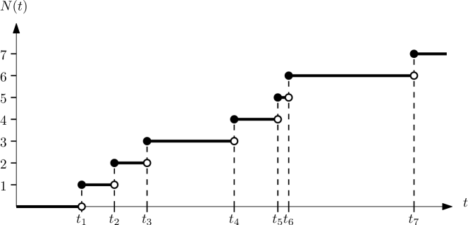
The counting and point process terminology is often interchangeable. For example, if one refers to a Poisson process or a HP then the reader must infer from the context whether the counting process or the point process of times is being discussed.
One way to characterise a particular point process is to specify the distribution function of the next arrival time conditional on the past. Given the history up until the last arrival , , define (as per ozaki1979 ) the conditional cumulative distribution function (c.d.f.) (and probability density function (p.d.f.)) of the next arrival time as
The joint p.d.f. for a realisation is then, by the chain rule,
| (1) |
In the literature the notation rarely specifies explicitly, but rather a superscript asterisk is used (see for example daley2003a ). We follow this convention and abbreviate and to and , respectively.
Remark 1
The function can be used to classify certain classes of point processes. For example, if a point process has an which is independent of then the process is a renewal process.
2.2 Conditional intensity functions
Often it is difficult to work with the conditional arrival distribution . Instead, another characterisation of point processes is used: the conditional intensity function. Indeed if the conditional intensity function exists it uniquely characterises the finite-dimensional distributions of the point process (see Proposition 7.2.IV of daley2003a ). Originally this function was called the hazard function cox1955 and was defined as
| (2) |
Although this definition is valid, we prefer an intuitive representation of the conditional intensity function as the expected rate of arrivals conditioned on :
Definition 3 (Conditional intensity function)
Consider a counting process with associated histories . If a (non-negative) function exists such that
which only relies on information of in the past (that is, is -measurable), then it is called the conditional intensity function of .
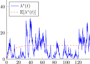
The terms ‘self-exciting’ and ‘self-regulating’ can be made precise by using the conditional intensity function. If an arrival causes the conditional intensity function to increase then the process is said to be self-exciting. This behaviour causes temporal clustering of . In this setting must be chosen to avoid explosion, where we use the standard definition of explosion as the event that for . See Fig. 2 for an example realisation of such a .
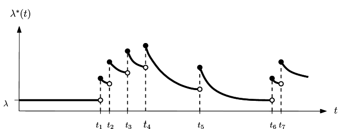
Alternatively, if the conditional intensity function drops after an arrival the process is called self-regulating and the arrival times appear quite temporally regular. Such processes are not examined hereafter, though an illustrative example would be the arrival of speeding tickets to a driver over time (assuming each arrival causes a period of heightened caution when driving).
2.3 Compensators
Frequently the integrated conditional intensity function is needed (for example, in parameter estimation and goodness of fit testing); it is defined as follows.
Definition 4 (Compensator)
For a counting process the non-decreasing function
is called the compensator of the counting process.
In fact, a compensator is usually defined more generally and exists even when does not exist. Technically is the unique predictable function, with , and is non-decreasing, such that almost surely for and where is an local martingale, whose existence is guaranteed by the Doob–Meyer decomposition theorem. However, for HPs always exists (in fact, as we shall see in Section 3, a HP is defined in terms of this function) and therefore Definition 4 is sufficient for our purposes.
3 Literature review
With essential background and core concepts outlined in Section 2, we now turn to discussing HPs, including their useful immigration–birth representation. We briefly touch on generalisations, before turning to a illustrative account of HPs for financial applications.
3.1 The Hawkes process
Point processes gained a significant amount of attention in the field of statistics during the 1950s and 1960s. First, Cox cox1955 introduced the notion of a doubly stochastic Poisson process (now called the Cox process) and Bartlett bartlett1963spectral ; bartlett1963density ; bartlett1964 investigated statistical methods for point processes based on their power spectral densities. At IBM Research Laboratories, Lewis lewis1964 formulated a point process model (for computer failure patterns) which was a step in the direction of the HP. The activity culminated in the significant monograph by Cox and Lewis cox1966 on time series analysis; modern researchers appreciate this text as an important development of point process theory since it canvassed their wide range of applications (daley2003a, , p. 16).
It was in this context that Hawkes hawkes1971spectra set out to bring Bartlett’s spectral analysis approach to a new type of process: a self-exciting point process. The process Hawkes described was a one-dimensional point process (though originally specified for as opposed to ), and is defined as follows.
Definition 5 (Hawkes process)
Consider a counting process, with associated history , that satisfies
Suppose the process’ conditional intensity function is of the form
| (3) |
for some and which are called the background intensity and excitation function respectively. Assume that to avoid the trivial case, that is, a homogeneous Poisson process. Such a process is a Hawkes process.
Remark 2
[]
\sidesubfloat[]
Remark 3
A realisation of a HP is shown in Fig. 3 with the associated path of the conditional intensity process. Hawkes hawkes1971point soon extended this single point process into a collection of self- and mutually-exciting point processes, which we will turn to discussing after elaborating upon this one-dimensional process.
3.2 Hawkes conditional intensity function
The form of the Hawkes conditional intensity function in (3) is consistent with the literature though it somewhat obscures the intuition behind it. Using to denote the observed sequence of past arrival times of the point process up to time , the Hawkes conditional intensity is
The structure of this is quite flexible and only requires specification of the background intensity and the excitation function . A common choice for the excitation function is one of exponential decay; Hawkes hawkes1971spectra originally used this form as it simplified his theoretical derivations hautsch2011 . In this case , which is parameterised by constants , and hence
| (4) |
The constants and have the following interpretation: each arrival in the system instantaneously increases the arrival intensity by , then over time this arrival’s influence decays at rate .
Another frequent choice for is a power law function, giving
with some positive scalars and . The power law form was popularised by the geological model called Omori’s law, used to predict the rate of aftershocks caused by an earthquake ogata1999 . More computationally efficient than either of these excitation functions is a piecewise linear function as in chatalbashev2007 . However, the remaining discussion will focus on the exponential form of the excitation function, sometimes referred to as the HP with exponentially decaying intensity.
One can consider the impact of setting an initial condition , perhaps in order to model a process from some time after it is started. In this scenario the conditional intensity process (using the exponential form of ) satisfies the stochastic differential equation
Applying stochastic calculus yields the general solution of
which is a natural extension of (4) dafonseca2014 .
3.3 Immigration–birth representation
Stability properties of the HP are often simpler to divine if it is viewed as a branching process. Imagine counting the population in a country where people arrive either via immigration or by birth. Say that the stream of immigrants to the country form a homogeneous Poisson process at rate . Each individual then produces zero or more children independently of one another, and the arrival of births form an inhomogeneous Poisson process.
An illustration of this interpretation can be seen in Fig. 4. In branching theory terminology, this immigration–birth representation describes a Galton–Watson process with a modified time dimension. Hawkes hawkes1974 used the representation to derive asymptotic characteristics of the process, such as the following result.
Theorem 3.1 (Hawkes process asymptotic normality)
Remark 4
More modern work uses the immigration–birth representation for applying Bayesian techniques; see, for example, rasmussen2013 .

For an individual who enters the system at time , the rate at which they produce offspring at future times is . Say that the direct offspring of this individual comprise the first-generation, and their offspring comprise the second-generation, and so on; members of the union of all these generations are called the descendants of this arrival.
Using the notation from (grimmett2001, , Section 5.4), define to be the random number of offspring in the th generation (with ). As the first-generation offspring arrived from a Poisson process where the mean is known as the branching ratio. This branching ratio (which can take values in ) is defined in Theorem 3.1 and in the case of an exponentially decaying intensity is
| (5) |
Knowledge of the branching ratio can inform development of simulation algorithms. For each immigrant , the times of the first-generation offspring arrivals—conditioned on knowing the total number of them —are each independent and identically distributed (i.i.d.) with density . Section 6 explores HP simulation methods inspired by the immigration–birth representation in more detail.
The value of also determines whether or not the HP explodes. To see this, let . A renewal-type equation will be constructed for and then its limiting value will be determined. Conditioning on the time of the first jump,
In order to calculate this expected value, start with
and take expectations (and apply the tower property)
to see that
Therefore
This renewal–type equation (in convolution notation is ) then has different solutions according to the value of . Asmussen asmussen2003 splits the cases into: the defective case (), the proper case (), and the excessive case (). Asmussen’s Proposition 7.4 states that for the defective case
| (6) |
However in the excessive case, exponentially quickly, and hence eventually explodes a.s.
Explosion for is supported by viewing the arrivals as a branching process. Since (see Section 5.4 Lemma 2 of grimmett2001 ), the expected number of descendants for one individual is
Therefore means that one immigrant would generate infinitely many descendants on average.
When the branching ratio can be interpreted as a probability. It is the ratio of the number of descendants for one immigrant, to the size of their entire family (all descendants plus the original immigrant); that is
Therefore, any HP arrival selected at random was generated endogenously (a child) with probability (w.p.) or exogenously (an immigrant) w.p. . Most properties of the HP rely on the process being stationary, which is another way to insist that (a rigorous definition is given in Section 3.4), so this is assumed hereinafter.
3.4 Covariance and power spectral densities
HPs originated from the spectral analysis of general stationary point processes. The HP is stationary for finite values of when it is defined as per Remark 2, so we will use this definition for the remainder of Subsection 3.4. Finding the power spectral density of the HP gives access to many techniques from the spectral analysis field; for example, model fitting can be achieved by using the observed periodogram of a realisation. The power spectral density is defined in terms of the covariance density. Once again the exposition is simplified by using the shorthand that
Unfortunately the term ‘stationary’ has many different meanings in probability theory. In this context the HP is stationary when the jump process —which takes values in —is weakly stationary. This means that and do not depend on . Stationarity in this sense does not imply stationarity of or stationarity of the inter-arrival times lewis1970 . One consequence of stationarity is that will have a long term mean (as given by (6))
| (7) |
The (auto)covariance density is defined, for , to be
Due to the symmetry of covariance, , however cannot be extended to the whole of because there is an atom at . For simple point processes (since ) therefore for
The complete covariance density (complete in that its domain is all of ) is defined as
| (8) |
where is the Dirac delta function.
Remark 5
Typically is defined such that is everywhere continuous. Lewis (lewis1970, , p. 357) states that strictly speaking “does not have a ‘value’ at ”. See bartlett1963density ; cox1966 , and hawkes1971spectra for further details.
The corresponding power spectral density function is then
| (9) |
Up to now the discussion (excluding the final value of (7)) has considered general stationary point processes. To apply the theory specifically to HPs we need the following result.
Theorem 3.2 (Hawkes process power spectral density)
Consider a HP with an exponentially decaying intensity with . The intensity process then has covariance density, for ,
Hence, its power spectral density is, ,
Proof
(Adapted from hawkes1971spectra .) Consider the covariance density for :
| (10) |
Firstly note that, via the tower property,
Hence (10) can be combined with (3) to see that equals
which yields
| (11) |
Refer to Appendix A.1 for details; this is a Wiener–Hopf-type integral equation. Taking the Laplace transform of (3.4) gives
Refer to Appendix A.2 for details. Note that (5) and (7) supply , which implies that
Therefore,
The values of and are then substituted into the definition given in (9):
Remark 7
As is a real-valued symmetric function, its Fourier transform is also real-valued and symmetric, that is,
and
It is common that is plotted instead of , as in Section 4.5 of cox1966 ; this is equivalent to wrapping the negative frequencies over to the positive half-line.
3.5 Generalisations
The immigration–birth representation is useful both theoretically and practically. However it can only be used to describe linear HPs. Brémaud and Massoulié bremaud1996 generalised the HP to its nonlinear form:
Definition 6 (Nonlinear Hawkes process)
Modern work on nonlinear HPs is much rarer than the original linear case (for simulation see pp. 96–116 of carstensen2010 , and associated theory in zhu2013 ). This is due to a combination of factors; firstly, the generalisation was introduced relatively recently, and secondly, the increased complexity frustrates even simple investigations.
Now to return to the extension mentioned earlier, that of a collection of self- and mutually-exciting HPs. The processes being examined are collections of one-dimensional HPs which ‘excite’ themselves and each other.
Definition 7 (Mutually exciting Hawkes process)
Consider a collection of counting processes , denoted . Say are the random arrival times for each counting process (and for observed arrivals). If for each then has conditional intensity of the form
| (12) |
for some and , then is called a mutually exciting Hawkes process.
When the excitation functions are set to be exponentially decaying, (12) can be written as
| (13) |
for non-negative constants .
3.6 Financial applications
This section reviews primarily the work of Aït-Sahalia, et al. ait2010 and Filimonov and Sornette filimonov2012 . It assumes the reader is familiar with mathematical finance and the use of stochastic differential equations.
3.6.1 Financial contagion
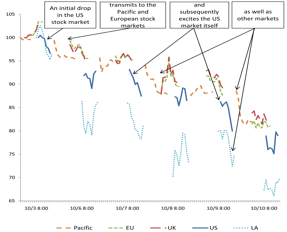
We turn our attention to the moest recent applications of HPs. A major domain for self- and mutually-exciting processes is financial analysis. Frequently it is seen that large movements in a major stock market propagate in foreign markets as a process called financial contagion. Examples of this phenomenon are clearly visible in historical series of asset prices; Fig. 5 illustrates one such case.
The ‘Hawkes diffusion model’ introduced by ait2010 is an attempt to extend previous models of stock prices to include financial contagion. Modern models for stock prices are typically built upon the model popularised by black1973 where the log returns on the stock follow geometric Brownian motion. Whilst this seminal paper was lauded by the economics community, the model inadequately captured the ‘fat tails’ of the return distribution and so was not commonly used by traders haug2009 . Merton merton1976 attempted to incorporate heavy tails by including a Poisson jump process to model booms and crashes in the stock returns; this model is often called Merton diffusion model. The Hawkes diffusion model extends this model by replacing the Poisson jump process with a mutually-exciting HP, so that crashes can self-excite and propagate in a market and between global markets.
The basic Hawkes diffusion model describes the log returns of assets where each asset has associated expected return , constant volatility , and standard Brownian motion . The Brownian motions have constant correlation coefficients . Jumps are added by a self- and mutually-exciting HP (as per Definition 7 with some selection of constants and ) with stochastic jump sizes . The asset dynamics are then assumed to satisfy
The general Hawkes diffusion model replaces the constant volatilities with stochastic volatilities specified by the Heston model. Each asset has a: long-term mean volatility , rate of returning to this mean , volatility of the volatility , and standard Brownian motion . Correlation between the ’s is optional, yet the effect would be dominated by the jump component. Then the full dynamics are captured by
However the added realism of the Hawkes diffusion model comes at a high price. The constant volatility model requires parameters to be fit (assuming is characterised by two parameters) and the stochastic volatility extension requires an extra parameters (assuming that ). In ait2010 hypothesis tests reject the Merton diffusion model in favour of the Hawkes diffusion model, however there are no tests for overfitting the data (for example, Akaike or Bayesian information criterion comparisons). Remember that John Von Neumann (reputedly) claimed that “with four parameters I can fit an elephant” dyson2004 .
For computational necessity the authors made a number of simplifying assumptions to reduce the number of parameters to fit (such as the background intensity of crashes is the same for all markets). Even so, the Hawkes diffusion model was only able to be fitted for pairs of markets () instead of for the globe as a whole. Since the model was calibrated to daily returns of market indices, historical data was easily available (for exmaple, from Google or Yahoo! finance); care had to be taken to convert timezones and handle the different market opening and closing times. The parameter estimation method used by ait2010 was the generalised method of moments, however the theoretical moments derived satisfy long and convoluted equations.
3.6.2 Mid-price changes and high-frequency trading
A simpler system to model is a single stock’s price over time, though there are many different prices to consider. For each stock one could use: the last transaction price, the best ask price, the best bid price, or the mid-price (defined as the average of best ask and best bid prices). The last transaction price includes inherent microstructure noise (for example, the bid–ask bounce), and the best ask and bid prices fail to represent the actions of both buyers and sellers in the market.
Filimonov and Sornette filimonov2012 model the mid-price changes over time as a HP. In particular they look at long-term trends of the (estimated) branching ratio. In this context, represents the proportion of price moves that are not due to external market information but simply reactions to other market participants. This ratio can be seen as the quantification of the principle of economic reflexivity. The authors conclude that the branching ratio has increased dramatically from in 1998 to in 2007.
Later that year lorenzen2012 critiqued the test procedure used in this analysis. Filimonov and Sornette filimonov2012 had worked with a dataset with timestamps accurate to a second, and this often led to multiple arrivals nominally at the same time (which is an impossible event for simple point processes). Fake precision was achieved by adding Unif random fractions of seconds to all timestamps, a technique also used by bowsher2007 . Lorenzen found that this method added an element of smoothing to the data which gave it a better fit to the model than the actual millisecond precision data. The randomisation also introduced bias to the HP parameter estimates, particularly of and . Lorenzen formed a crude measure of high-frequency trading activity leading to an interesting correlation between this activity and over the observed period.
Remark 9
Fortunately we have received comments from referees suggesting other very important works to consider, which we will briefly list here. The importance of Bowsher bowsher2007 is highlighted, as is the series by Chavez-Demoulin et al. chavez2005 ; chavez2012 . They point to the book by McNeil et al. mcneil2015 where a section is devoted to HP applications, and stress the relevance of the Parisian school in applying HPs to microstructure modelling, for example, the paper by Bacry et al. bacry2013 .
4 Parameter estimation
This section investigates the problem of generating parameters estimates given some finite set of arrival times presumed to be from a HP. For brevity, the notation here will omit the and arguments from functions: , , , and . The estimators are tested over simulated data, for the sake of simplicity and lack of relevant data. Unfortunately this method bypasses the many significant challenges raised by real datasets, challenges that caused filimonov2013 to state that
“Our overall conclusion is that calibrating the Hawkes process is akin to an excursion within a minefield that requires expert and careful testing before any conclusive step can be taken.”
The method considered is maximum likelihood estimation, which begins by finding the likelihood function, and estimates the model parameters as the inputs which maximise this function.
4.1 Likelihood function derivation
Daley and Vere-Jones (daley2003a, , Proposition 7.2.III) give the following result.
Theorem 4.1 (Hawkes process likelihood)
Let be a regular point process on for some finite positive , and let denote a realisation of over . Then, the likelihood of is expressible in the form
Proof
First assume that the process is observed up to the time of the th arrival. The joint density function from (1) is
This function can be written in terms of the conditional intensity function. Rearrange (2) to find in terms of (as per rasmussen2009 ):
Integrate both sides over the interval :
The HP is a simple point process, meaning that multiple arrivals cannot occur at the same time. Hence as , and so
| (14) |
Further rearranging yields
| (15) |
Thus the likelihood becomes
| (16) |
Now suppose that the process is observed over some time period . The likelihood will then include the probability of seeing no arrivals in the time interval :
Using the formulation of from (15), then
The completes the proof.
4.2 Simplifications for exponential decay
With the likelihood function from (16), the log-likelihood for the interval can be derived as
| (17) |
Note that the integral over can be broken up into the segments , , , , and therefore
This can be simplified in the case where decays exponentially:
Finally, many of the terms of this double summation cancel out leaving
| (18) |
Note that here the final summand is unnecessary, though it is often included, see lorenzen2012 . Substituting and into (17) gives
| (19) |
This direct approach is computationally infeasible as the first term’s double summation entails complexity. Fortunately the similar structure of the inner summations allows to be computed with complexity ogata1978 ; crowley2013 . For , let , so that
| (20) |
With the added base case of , can be rewritten as
| (21) |
Ozaki ozaki1979 also gives the partial derivatives and the Hessian for this log-likelihood function. Of particular note is that each derivative calculation can be achieved in order complexity when a recursive approach (similar to (20)) is taken ogata1981 .
Remark 10
The recursion implies that the joint process is Markovian (see Remark 1.22 of liniger2009 ).
4.3 Discussion
Understanding of the maximum likelihood estimation method for the HP has changed significantly over time. The general form of the log-likelihood function (17) was known by Rubin rubin1972 . It was applied to the HP by Ozaki ozaki1979 who derived (19) and the improved recursive form (21). Ozaki also found (as noted earlier) an efficient method for calculating the derivatives and the Hessian matrix. Consistency, asymptotic normality and efficiency of the estimator were proved by Ogata ogata1978 .
It is clear that the maximum likelihood estimation will usually be very effective for model fitting. However, filimonov2012 found that, for small samples, the estimator produces significant bias, encounters many local optima, and is highly sensitive to the selection of excitation function. Additionally, the complexity can render the method useless when samples become large; remember that any iterative optimisation routine would calculate the likelihood function perhaps thousands of times. The R ‘hawkes’ package thus implements this routine in C++ in an attempt to mitigate the performance issues.
This ‘performance bottleneck’ is largely the cause of the latest trend of using the generalised method of moments to perform parameter estimation. Da Fonseca and Zaatour dafonseca2014 state that the procedure is “instantaneous” on their test sets. The method uses sample moments and the sample autocorrelation function which are smoothed via a (rather arbitrary) user-selected procedure.
5 Goodness of fit
This section outlines approaches to determining the appropriateness of a HPs model for point data, which is a critical link in their application.
5.1 Transformation to a Poisson process
Assessing the goodness of fit for some point data to a Hawkes model is an important practical consideration. In performing this assessment the point process’ compensator is essential, as is the random time change theorem (here adapted from brown2002 ):
Theorem 5.1 (Random time change theorem)
Say is a realisation over time from a point process with conditional intensity function . If is positive over and a.s. then the transformed points form a Poisson process with unit rate.
The random time change theorem is fundamental to the model fitting procedure called (point process) residual analysis. Original work embrechts2011 on residual analysis goes back to meyer1971 , papangelou1972 , and watanabe1964 . Daley and Vere-Jones’s Proposition 7.4.IV daley2003a rewords and extends the theorem as follows.
Theorem 5.2 (Residual analysis)
Consider an unbounded, increasing sequence of time points in the half-line , and a monotonic, continuous compensator such that a.s. The transformed sequence , whose counting process is denoted , is a realisation of a unit rate Poisson process if and only if the original sequence is a realisation from the point process defined by .
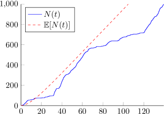
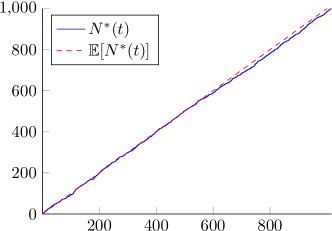
Hence, equipped with a closed form of the compensator from (18), the quality of the statistical inference can be ascertained using standard fitness tests for Poisson processes. Fig. 6 shows a realisation of a HP and the corresponding transformed process. In Fig. 6 appears identical to . They are actually slightly different ( is continuous) however the similarity is expected due to Doob–Meyer decomposition of the compensator.
[] \sidesubfloat[]
\sidesubfloat[] 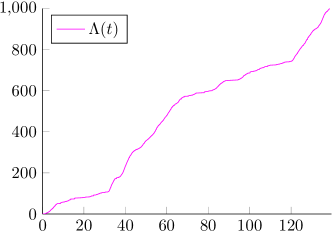 \sidesubfloat[]
5.2 Tests for Poisson process
5.2.1 Basic tests
There are many procedures for testing whether a series of points form a Poisson process (see cox1966 for an extensive treatment). As a first test, one can run a hypothesis test to check . If this initial test succeeds then the interarrival times,
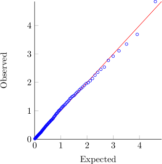
should be tested to ensure . A qualitative approach is to create a quantile–quantile (Q–Q) plot for using the exponential distribution (see for example Fig. 7). Otherwise a quantitative alternative is to run Kolmogorov–Smirnov (or perhaps Anderson–Darling) tests.
5.2.2 Test for independence
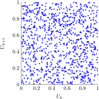
The next test, after confirming there is reason to believe that the are exponentially distributed, is to check their independence. This can be done by looking for autocorrelation in the sequence. Obviously zero autocorrelation does not imply independence, but a non-zero amount would certainly imply a non-Poisson model. A visual examination can be conducted by plotting the points . If there are noticeable patterns then the are autocorrelated. Otherwise the points should look evenly scattered; see for example Fig. 7. Quantitative extensions exist; for example see Section 3.3.3 of knuth2014 , or serial correlation tests in kroese2011 .
[] \sidesubfloat[]
5.2.3 Lewis test
A statistical test with more power is the Lewis test as described by kim2013 . Firstly, it relies on the fact that if are arrival times for a unit rate Poisson process then are distributed as the order statistics of a uniform random sample. This observation is called conditional uniformity, and forms the basis for a test itself. Lewis’ test relies on applying Durbin’s modification (introduced in durbin1961 with a widely applicable treatment by lewis1965 ).
5.2.4 Brownian motion approximation test
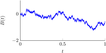
An approximate test for Poissonity can be constructed by using the Brownian motion approximation to the Poisson process. This is to say, the observed times are transformed to be (approximately) Brownian motion, and then known properties of Brownian motion sample paths can be used to accept or reject the original sample.
The motivation for this line of enquiry comes from Algorithm 7.4.V of daley2003a , which is described as an “approximate Kolmogorov–Smirnov-type test”. Unfortunately, a typographical error causes the algorithm (as printed) to produce incorrect answers for various significance levels. An alternative test based on the Brownian motion approximation is proposed here.
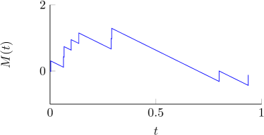
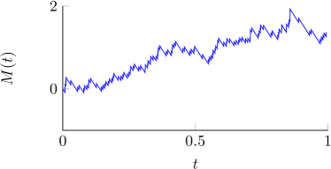
Say that is a Poisson process of rate . Define for . Donsker’s invariance principle implies that, as , converges in distribution to standard Brownian motion . Fig. 8 shows example realisations of for various that, at least qualitatively, are reasonable approximations to standard Brownian motion.
An alternative test is to utilise the first arcsine law for Brownian motion, which states that the random time , given by
is arcsine distributed (that is, ). Therefore the test takes a sequence of arrivals observed over and:
-
1.
transforms the arrivals to which should be a Poisson process with rate over ,
-
2.
constructs the Brownian motion approximation as above, finds the maximiser , and
-
3.
accepts the ‘unit-rate Poisson process’ hypothesis if lies within the quantiles of the distribution; otherwise it is rejected.
As a final note, many other tests can be performed based on other properties of Brownian motion. For example, the test could be based simply on noting that , and thus accepts if and rejects otherwise.
[] \sidesubfloat[]
\sidesubfloat[]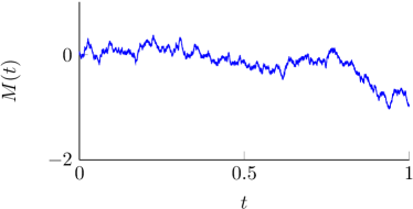 \sidesubfloat[]
6 Simulation methods
Simulation is an increasingly indispensable tool in probability modelling. Here we give details of three fundamental approaches to producing realisations of HPs.
6.1 Transformation methods
For general point processes a simulation algorithm is suggested by the converse of the random time change theorem (given in Section 5.1). In essence, a unit rate Poisson process is transformed by the inverse compensator into any general point process defined by that compensator. The method, sometimes called the inverse compensator method, iteratively solves the equations
for , the desired point process (see giesecke2005 and Algorithm 7.4.III of daley2003a ).
For HPs the algorithm was first suggested by Ozaki ozaki1979 , but did not state explicitly any relation to time changes. It instead focused on (14),
which relates the conditional c.d.f. of the next arrival to the previous history of arrivals and the specified . This relation means the next arrival time can easily be generated by the inverse transform method, that is draw then is found by solving
| (22) |
For an exponentially decaying intensity the equation becomes
Solving for can be achieved in linear time using the recursion of (20). However if a different excitation function is used then (22) must be solved numerically, for example using Newton’s method ogata1981 , which entails a significant computational effort.
6.2 Ogata’s modified thinning algorithm
HP generation is a similar problem to inhomogeneous Poisson process generation. The standard way to generate a inhomogeneous Poisson process driven by intensity function is via thinning. Formally the process is described by Algorithm 1 lewis1979 . The intuition is to generate a ‘faster’ homogeneous Poisson process, and remove points probabilistically so that the remaining points satisfy the time-varying intensity . The first process’ rate cannot be less than over .
A similar approach can be used for the HP, called Ogata’s modified thinning algorithm ogata1981 ; liniger2009 . The conditional intensity does not have an a.s. asymptotic upper bound, however it is common for the intensity to be non-increasing in periods without any arrivals. This implies that for , (that is, the time just after , when that arrival has been registered). So the value can be updated during each simulation. Algorithm 2 describes the process and Fig. 9 shows an example of each thinning procedure.
[]
\sidesubfloat[]
6.3 Superposition of Poisson processes
The immigration–birth representation gives rise to a simple simulation procedure: generate the immigrant arrivals, then generate the descendants for each immigrant. Algorithm 3 describes the procedure in full, with Fig. 10 showing an example realisation.
Immigrants form a homogeneous Poisson process of rate , so over an interval the number of immigrants is Poi() distributed. Conditional on knowing that there are immigrants, their arrival times are distributed as the order statistics of i.i.d. Unif[] random variables.
Each immigrant’s descendants form an inhomogeneous Poisson process. The th immigrant’s descendants arrive with intensity for . Denote to be the number of descendants of immigrant , then , and hence . Say that the descendants of the th immigrant arrive at times . Conditional on knowing , the are i.i.d. random variables distributed with p.d.f. . For exponentially decaying intensities, this simplifies to .
[]
\sidesubfloat[]
6.4 Other methods
This section’s contents are by no means a complete compilation of simulation techniques available for HPs. Dassios and Zhao dassios2013 and Møller and Rasmussen moller2005 give alternatives to the methods listed above. Also not discussed is the problem of simulating mutually-exciting HPs, however there are many free software packages that provide this functionality. Fig. 11 shows an example realisation generated using the R package ‘hawkes’ (see also Roger D. Peng’s related R package ‘ptproc’).
[]
\sidesubfloat[]
7 Conclusion
HPs are fundamentally fascinating models of reality. Many of the standard probability models are Markovian and hence disregard the history of the process. The HP is structured around the premise that the history matters, which partly explains why they appear in such a broad range of applications.
If the exponentially decaying intensity can be utilised, then the joint process satisfies the Markov condition, and both processes exhibit amazing analytical tractability. Explosion is avoided by ensuring that . The covariance density is a simple symmetric scaled exponential curve, and the power spectral density is a shifted scaled Cauchy p.d.f. The likelihood function and the compensator are elegant, and efficient to calculate using recursive structures. Exact simulation algorithms can generate this type of HP with optimal efficiency. Many aspects of the HP remain obtainable with any selection of excitation function; for example, the random time change theorem completely solves the problem of testing the goodness of a model’s fit.
The use of HPs in finance appears itself to have been a self-exciting process. Aït-Sahalia et al. ait2010 , Filimonov and Sornette filimonov2012 , and Da Fonseca and Zaatour dafonseca2014 formed the primary sources for the financial part of Section 3; these papers are surprisingly recent (given the fact that the model was introduced in 1971) and are representative of a current surge in HP research.
Appendix A Additional proof details
In this appendix, we collect additional detail elided from the proof of Theorem 3.2.
A.1 Supplementary to Theorem 3.2 (part one)
A.2 Supplementary to Theorem 3.2 (part two)
References
- (1) Y. Ogata, Journal of the American Statistical Association 83(401), 9 (1988)
- (2) G.O. Mohler, M.B. Short, P.J. Brantingham, F.P. Schoenberg, G.E. Tita, Journal of the American Statistical Association 106(493), 100 (2011)
- (3) S. Azizpour, K. Giesecke, G. Schwenkler. Exploring the sources of default clustering. http://web.stanford.edu/dept/MSandE/cgi-bin/people/faculty/giesecke/pdfs/exploring.pdf (2010). Working paper, retrieved on 10 Feb 2015
- (4) A.G. Hawkes, Biometrika 58(1), 83 (1971)
- (5) D. Lando, M.S. Nielsen, Journal of Financial Intermediation 19(3), 355 (2010)
- (6) V. Filimonov, D. Sornette, Physical Review E 85(5), 056108 (2012)
- (7) L. Carstensen, Hawkes processes and combinatorial transcriptional regulation. Ph.D. thesis, University of Copenhagen (2010)
- (8) T. Ozaki, Annals of the Institute of Statistical Mathematics 31(1), 145 (1979)
- (9) D. Daley, D. Vere-Jones, An Introduction to the Theory of Point Processes: Volume I: Elementary Theory and Methods (Springer, 2003)
- (10) D.R. Cox, Journal of the Royal Statistical Society. Series B (Methodological) 17(2), 129 (1955)
- (11) M.S. Bartlett, Journal of the Royal Statistical Society. Series B (Methodological) 25(2), 264 (1963)
- (12) M.S. Bartlett, Sankhyā: The Indian Journal of Statistics, Series A 25(3), 245 (1963)
- (13) M.S. Bartlett, Biometrika 51(3/4), 299 (1964)
- (14) P.A. Lewis, Journal of the Royal Statistical Society. Series B (Methodological) 26(3), 398 (1964)
- (15) D.R. Cox, P.A. Lewis, The Statistical Analysis of Series of Events (Monographs on Applied Probability and Statistics, London: Chapman and Hall, 1966)
- (16) A.G. Hawkes, Journal of the Royal Statistical Society. Series B (Methodological) 33(3), 438 (1971)
- (17) N. Hautsch, Econometrics of Financial High-Frequency Data (Springer, 2011)
- (18) Y. Ogata, Pure and Applied Geophysics 155(2/4), 471 (1999)
- (19) V. Chatalbashev, Y. Liang, A. Officer, N. Trichakis. Exciting times for trade arrivals. http://users.iems.northwestern.edu/ armbruster/2007msande444/report1a.pdf (2007). Stanford University MS&E 444 group project submission, retrieved on 10 Feb 2015
- (20) J. Da Fonseca, R. Zaatour, Journal of Futures Markets 34(6), 548 (2014)
- (21) A.G. Hawkes, D. Oakes, Journal of Applied Probability 11(3), 493 (1974)
- (22) J.G. Rasmussen, Methodology and Computing in Applied Probability 15(3), 623 (2013)
- (23) G. Grimmett, D. Stirzaker, Probability and Random Processes (Oxford University Press, 2001)
- (24) S. Asmussen, Applied Probability and Queues, 2nd edn. Applications of Mathematics: Stochastic Modelling and Applied Probability (Springer, 2003)
- (25) P.A. Lewis, Journal of Sound and Vibration 12(3), 353 (1970)
- (26) P. Brémaud, L. Massoulié, The Annals of Probability 24(3), 1563 (1996)
- (27) L. Zhu, Journal of Applied Probability 50(3), 760 (2013)
- (28) Y. Aït-Sahalia, J. Cacho-Diaz, R.J. Laeven, Modeling financial contagion using mutually exciting jump processes. Tech. Rep. 15850, National Bureau of Economic Research, USA (2010)
- (29) F. Black, M. Scholes, The Journal of Political Economy 81(3), 637 (1973)
- (30) E.G. Haug, N.N. Taleb, Wilmott Magazine 71 (2014)
- (31) R.C. Merton, Journal of Financial Economics 3(1), 125 (1976)
- (32) F. Dyson, Nature 427(6972), 297 (2004)
- (33) F. Lorenzen, Analysis of order clustering using high frequency data: A point process approach. Ph.D. thesis, Swiss Federal Institute of Technology Zurich (ETH Zurich) (2012)
- (34) C.G. Bowsher, Journal of Econometrics 141(2), 876 (2007)
- (35) V. Chavez-Demoulin, A.C. Davison, A.J. McNeil, Quantitative Finance 5(2), 227 (2005)
- (36) V. Chavez-Demoulin, J. McGill, Journal of Banking & Finance 36(12), 3415 (2012)
- (37) A.J. McNeil, R. Frey, P. Embrechts, Quantitative Risk Management: Concepts, Techniques and Tools: Concepts, Techniques and Tools (Princeton university press, 2015)
- (38) E. Bacry, S. Delattre, M. Hoffmann, J.F. Muzy, Quantitative Finance 13(1), 65 (2013)
- (39) V. Filimonov, D. Sornette, Apparent criticality and calibration issues in the Hawkes self-excited point process model: application to high-frequency financial data. Tech. Rep. 13-60, Swiss Finance Institute Research Paper (2013)
- (40) J.G. Rasmussen. Temporal point processes: the conditional intensity function. http://people.math.aau.dk/ jgr/teaching/punktproc11/tpp.pdf (2009). Course notes for ‘rumlige punktprocesser’ (spatial point processes), retrieved on 10 Feb 2015
- (41) Y. Ogata, Annals of the Institute of Statistical Mathematics 30(1), 243 (1978)
- (42) S. Crowley. Point process models for multivariate high-frequency irregularly spaced data. http://vixra.org/pdf/1211.0094v6.pdf (2013). Working paper, retrieved on 10 Feb 2015
- (43) Y. Ogata, Information Theory, IEEE Transactions on 27(1), 23 (1981)
- (44) T.J. Liniger, Multivariate Hawkes processes. Ph.D. thesis, Swiss Federal Institute of Technology Zurich (ETH Zurich) (2009)
- (45) I. Rubin, Information Theory, IEEE Transactions on 18(5), 547 (1972)
- (46) E. Brown, R. Barbieri, V. Ventura, R. Kass, L. Frank, Neural computation 14(2), 325 (2002)
- (47) P. Embrechts, T. Liniger, L. Lin, Journal of Applied Probability 48A, 367 (2011). Special volume: a Festschrift for Søren Asmussen
- (48) P.A. Meyer, in Séminaire de Probabilités V Université de Strasbourg (Springer, 1971), pp. 191–195
- (49) F. Papangelou, Transactions of the American Mathematical Society 165, 483 (1972)
- (50) S. Watanabe, Japan. J. Math 34(53-70), 82 (1964)
- (51) D.E. Knuth, Art of Computer Programming, Volume 2: Seminumerical Algorithms, The (Addison-Wesley Professional, 2014)
- (52) D. Kroese, T. Taimre, Z.I. Botev, Handbook of Monte Carlo methods (Wiley, 2011)
- (53) S.H. Kim, W. Whitt, The power of alternative Kolmogorov–Smirnov tests based on transformations of the data (2013). Submitted to ACM Transactions on Modeling and Computer Simulation, Special Issue in Honor of Don Iglehart (Issue 25.4)
- (54) J. Durbin, Biometrika 53(3/4), 41 (1961)
- (55) P.A. Lewis, Biometrika 52(1/2), 67 (1965)
- (56) K. Giesecke, P. Tomecek. Dependent events and changes of time. http://web.stanford.edu/dept/MSandE/cgi-bin/people/faculty/giesecke/pdfs/dect.pdf (2005). Working paper, retrieved on 10 Feb 2015
- (57) P.A. Lewis, G.S. Shedler, Naval Research Logistics Quarterly 26(3), 403 (1979)
- (58) A. Dassios, H. Zhao, Electronic Communications in Probability 18(62) (2013)
- (59) J. Møller, J.G. Rasmussen, Advances in Applied Probability 37(3), 629 (2005)