Impact of Galactic magnetic field modelling on searches of point sources via UHECR-neutrino correlations

Abstract

We apply the Jansson-Farrar JF12 magnetic field configuration in the context of point source searches by correlating the Telescope Array ultra-high energy cosmic ray data and the IceCube-40 neutrino candidates, as well as other magnetic field hypotheses. Our field hypotheses are: no magnetic field, the JF12 field considering only the regular component, the JF12 full magnetic field, which is a combination of regular and random field components, and the standard turbulent magnetic field used in previous correlation analyses. As expected from a neutrino sample such as IceCube-40, consistent with atmospheric neutrinos, we have found no significant correlation signal in all the cases. Therefore, this paper is mainly devoted to the comparison of the effect of the different magnetic field hypotheses on the minimum neutrino source flux strength required for a $5\sigma$ discovery and the derived $90\%$ CL upper limits. We also incorporate in our comparison the cases of different power law indices $\alpha=2,\alpha=2.3$ for the neutrino point source flux. Our results indicate that the discovery potential for a point source search is sensitive to changes in the magnetic field assumptions, being the difference between the models mentioned before between 15% and 26%. Finally, as a collateral result, we implement a novel parameterisation of the JF12 random component.

I INTRODUCTION

One of the most important quests in particle astrophysics is to identify the sources that produce ultra-high energy cosmic rays (UHECR). One way to achieve this goal is to directionally correlate UHECR with astrophysical neutrinos. This correlation would not only indicate us the sites of hadronic acceleration, but also their non single-shot transient nature. On the other hand, a positive correlation signal requires sources producing a similar order of fluxes of UHECR (e.g.protons) and neutrinos. This condition is fulfilled by sources with a proton interaction opacity $\tau\gtrsim 1$. Meanwhile, sources with $\tau\ll 1$ or $\tau\gg 1$ would either produce almost exclusively protons with a small associated neutrino flux or produce only neutrinos, absorbing the corresponding protons, respectively. A mean free path length can be linked to the interaction between the protons escaping from the source and the Cosmic Microwave Background (CMB), defining the so called GZK sphere of radius $\sim 100$ Mpc  Greisen66 ; Zatsepin66 . This would give us the limit of the farthest distance of observable UHECR sources, an implicit condition for any correlation analysis.

One key ingredient in a directional correlation analysis between UHECR and neutrinos is to have an accurate determination of the UHECR magnetic deflection. Since the UHECR are charged particles, in their travel to Earth, they are going to be deflected due to its interaction with the magnetic field inside and outside the Galaxy, the latter being true if they are coming from an extragalactic source.

This type of analysis has been perfomed under different magnetic field hypotheses. Examples include correlation studies between UHECR from the Pierre Auger Observatory (PAO) and neutrino events from the ANTARES Telescope Martinez12 and between UHECR from Telescope Array (TA) and neutrino events from IceCube Fang14 . In all these analyses, an energy independent magnetic deflection has been used. This kind of estimation is reasonable since we are not certain about the description of the Galactic or the Extragalactic magnetic field. However, it is interesting to examine the impact on correlation analyses, calculating the magnetic deflections under different Galactic Magnetic field models, taking into account energy dependent considerations in their estimations. Following this idea, a study of cosmic ray deflections from Centaurus A was proposed in Keivani15 in which the more recent version of the Jansson and Farrar Jansson12a ; Jansson12b (JF12) magnetic field model has been implemented. The JF12 is an improved model of the Galactic magnetic field, including a regular and random field component. This model fits very well the WMAP7 Galactic synchrotron emission map and more than 40,000 extragalactic Faraday rotation measurements. The JF12 model also includes an out-of-plane component and striated-random fields.

In this work we use four different magnetic field hypotheses: no field, the regular component of the JF12, the full JF12 field model, and the standard turbulent magnetic field. These hypotheses are initially used to study the correlation between the Telescope Array ultra-high energy cosmic ray data Abbasi14 and the IceCube-40 neutrino candidates Abbasi11 . Since no correlation is expected, the main analysis of this paper is the comparison of the neutrino flux requirement for a $5\sigma$ discovery and the $90\%$ CL upper limits, under the four magnetic field hypotheses. The paper is divided as follows: in section 2 we describe the magnetic field models used in this study and we also present the parametrization that we have developed of the angular deflections from the random component of the JF12 field. In sections 3 and 4 we outline the method used to find correlations between UHECR and neutrinos and we describe how to include magnetic field deflections in our statistical analysis. In section 5 we present our results and in section 6 our conclusions.

II GALACTIC MAGNETIC FIELD MODELS

The angular deflection $\delta$ of an ultrarelativistic particle of charge $Ze$ and energy $E$ due to the magnetic field is described by:

$$\delta\propto\frac{Ze}{E}\left|\int\hat{\mathbf{p}}\times\mathbf{B}ds\right|$$ (1)

This formula reflects the inverse proportionality between $\delta$ and $E$ which is a key issue for understanding the parameterisation presented in section 3.

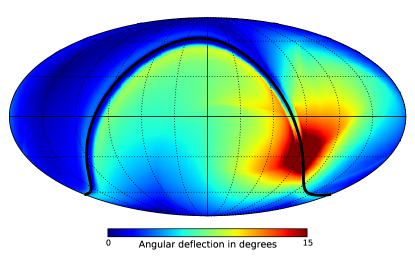
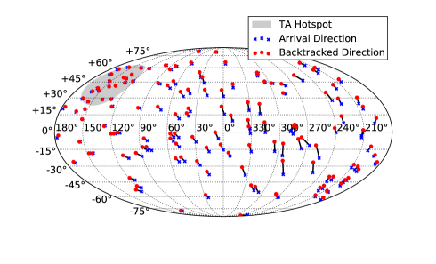
Figure 1: Top panel: Angular deflection from the regular component of the JF12 Field for a backtracked proton of energy $E=57$ EeV. The galactic plane is indicated by the thick black line. Map drawn using HEALPix Gorski05 . Bottom panel: Deflection of PAO and TA UHECR events under the regular component of the JF12 field. The shaded region marks the TA hotspot. Maps in equatorial coordinates.

The deflection of a charged particle as it travels through a turbulent extragalactic magnetic field (EGMF), with strength of order $~{}6$nG, is proportional to $\sqrt{D}|Z|/E$ where $D$ is the source distance, $Z$ the charge number of the UHECR and $E$ its energy Dolag04 ; Kotera & Lemoine (2008). These deflections are typically $\leq 1^{\circ}$ for protons with energy above 40 EeV and a propagation distance of order $\sim 1$ Gpc. Meanwhile, deflections caused by the galactic magnetic field (GMF), with strength of order $~{}6\mu$G, may be significant. In fact, this is particularly significant if the cosmic rays are composed by heavy nuclei such as iron and may be deflected by a few tens of degrees even for energies above $10^{20}$ eV.

For distances up to 500 Mpc and energies $E\geq 4\times 10^{19}$ eV, typical deflections from EGMF are smaller than the resolution of UHECR detectors (see, e.g., Dolag04 ). Thus, if the UHECR sources are within the GZK sphere of radius $\sim 100$ Mpc, we may neglect EGMF deflection for energies $E\geq 3\times 10^{19}$ eV, which is the case in our analysis.

Our correlation analysis is mainly tested under two different Galactic magnetic field models. One of these models is the JF12 GMF model Jansson12a ; Jansson12b , designed to fit the rotation measures and polarized synchrotron data, as we have already mentioned before. The JF12 model separates the magnetic field into three components: regular (coherent), striated and purely random fields (random components). All components extend up to $r=20$ kpc, where $r$ is the in-plane radius with origin at the galactic center. The regular component (or large-scale field) is a superposition of three fields: spiral disk field, toroidal halo field and the X-shaped poloidal halo field. Figure 1 shows the deflection from the coherent field for a backtracked 57 EeV proton. Deflections are stronger for backtracked directions below the Galactic plane and are strongest when the particle propagates across the galactic center.

In addition to the regular component of the JF12, the striated random field is fully aligned to all components of the regular field. The final component is an isotropic random small-scale field. The coherence length of these fields is expected to be of order 100 pc or less. The GMF will be modelled using the best-fit parameters in Jansson12a ; Jansson12b and assuming a coherence length of 60 pc for the fully random component.

The other model, which we denote by “standard”, was used in Ref. Martinez12 ; Lauer11 for similar UHECR-neutrino correlation studies. In this model the deflections follow a Gaussian distribution with width $3^{\circ}$. In Aab14 , this method was changed to a Fisher distribution with an energy dependent concentration parameter.

II.1 Random component parameterization of the JF12 GMF

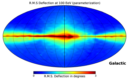
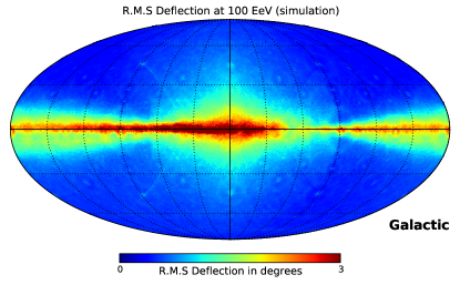
Figure 2: Left panel: R.M.S. deflection due to random field components for 100 EeV protons, using our parameterization (Eq. (5)). Right panel: The same plot by backtracking for several realizations of the full JF12 Field (simulation). Map drawn using HEALPix Gorski05 .

A secondary contribution of this work is the implementation of a parameterization of the random component of the JF12 GMF model. This analytic expression would help us in having a better insight into the behaviour of this component while saving computational time in the calculations of our analysis. This parametrization is valid for small deflections, a condition that restricts the energy range of UHECR, which are protons, to energies greater than 57 EeV. We have chosen protons with this energy since the deflections are going to be small, which is a requirement for our results to be valid. In addition, for the backtracking method, we have used CRPropa 3 Batista13 to propagate cosmic rays under the JF12 magnetic field model, using the best fit values given in Jansson12a , for the coherent field parameters, and in Jansson12b , for the random field parameters.

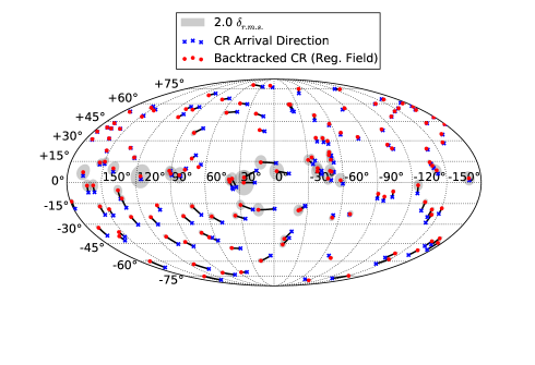
Figure 3: Deflection of the 69 UHECR reported by PAO in Abreu10 and the 72 TA events in Galactic coordinates. The blue crosses are the arrival directions of the cosmic rays as seen from Earth. The red dots correspond to the backtracked events using the regular component of the JF12 Field and each event is connected to its observed arrival direction by a black line. The gray circles have radii $2.0\;\delta_{\textrm{r.m.s}}$ (see Eq. (5)), which correspond to the additional deflection from the random components of the JF12 Field.

Our procedure for obtaining the parameterisation goes as follows: firstly, for a given initial arrival direction (observed at the Earth) $P_{0}=(l_{0},b_{0})$ of a proton with energy $E$, where $(l,b)$ are in the galactic coordinate system with $-180^{\circ}\leq l<180^{\circ}$ the galactic longitude and $-90^{\circ}\leq b\leq 90^{\circ}$ the galactic latitude, we backtrack it through the coherent field to the position $P_{c}=(l_{c},b_{c})$. The latter is the final position reached by the proton before it leaves the GMF. Secondly, starting again from $P_{0}$, we backtrack another proton with the same energy $E$ through the full magnetic field (coherent plus random) until it arrives to its final position $P=(l,b)$, before it exits the GMF. Then the angular distance $\delta$ between $P_{c}$ and $P$ is calculated. After repeating this process over different realizations of the random component of the field, we may construct a distribution of the angular distance $\delta$.

To functionally describe the deflection, we have followed Aab14 where the random field deflections are given by a Fisher distribution. Under the small deflection angle hypothesis, the probability distribution function $f$ of the random field deflections can be described by a Rayleigh distribution:

$$f(\delta)=2\lambda\delta\exp\left(-\lambda\delta^{2}\right)$$ (2)

where $\lambda=\lambda(E)|_{l_{0},b_{0}}$ is a fit parameter for a given $l_{0},b_{0}$. We find that the optimal energy dependence of $\lambda$ is of the form

$$\lambda|_{l_{0},b_{0}}(E)=A_{1}|_{l_{0},b_{0}}E+A_{2}|_{l_{0},b_{0}}E^{2}$$ (3)

This energy dependence was tested for energies 57 EeV$\leq E\leq$200 EeV by taking 15 energies logarithmically spaced in this interval. The parameters $A_{1},A_{2}$ are given on a $50\times 50$ grid distributed uniformly across $-180^{\circ}\leq l_{0}<180^{\circ}$ and $-0.9999\leq\sin(b_{0})\leq 0.9999$. Using the 2500 tabulated points as a sample, the weighted averages (weight $w_{i}=\cos(b_{i})$) are given by

$$\langle A_{1}\rangle\sim(0.1\pm 3.0)\times 10^{-3}\textrm{EeV}^{-1}$$

$$\langle A_{2}\rangle\sim(2.6\pm 1.9)\times 10^{-4}\textrm{EeV}^{-2}$$ (4)

The distribution $f$ also satisfies

$$\langle\delta\rangle=\frac{\sqrt{\pi}}{2\sqrt{\lambda}}\qquad\qquad\delta_{\textrm{r.m.s.}}=\sqrt{\langle\delta^{2}\rangle}=\frac{1}{\sqrt{\lambda}}$$ (5)

From Eq. (5) we see that the $\delta_{\textrm{r.m.s}}$ deflection decreases for higher energies being that for energies above 100 EeV it goes like $\lambda\approx A_{2}E^{2}$. The behaviour $\delta_{\textrm{r.m.s}}\propto E^{-1}$ is therefore recovered in the higher energy regime, in agreement with Eq. (1). In fact, this is the reason why there are no terms of order higher than $E^{2}$ in the expression for $\lambda$. In order to test our proposed parameterization, we display in Figure 2 a comparison between this one and the numerical simulations, which are based on Runge-Kutta methods for the $\delta_{\textrm{r.m.s.}}$ of 100 EeV protons. These simulations are performed over 640 realizations of the full JF12 field and with the sky divided into only 49152 arrival directions. It is clear the excellent agreement between our parameterization and the numerical calculations.

Using $f$ we can reduce the computational time by up to two orders of magnitude, in comparison with the numerical calculations. The function $f$ only gives information on the angular deflection $\delta$, leaving for each $\delta$ an allowed region, an annulus, for the final backtracked position. We assume a symmetrical distribution of the particles in the annulus.

In Figure 3 we show the effect of Galactic magnetic deflections on the 69 PAO UHECR events and 72 TA events. These deflections have been obtained due to the regular component, that produce a fixed separation, and the random component, depicted using our parameterization. It is evident how the greatest deflection given by the random component occurs mainly in the vicinity of the galactic plane.

III GENERAL SCHEME OF THE CORRELATION ANALYSIS

In order to calculate the correlations between IceCube neutrinos and TA UHECRs, we have followed the source stacking method outlined in Martinez12 . This method adds up the flux intensities from a group of single sources concentrated in a small region of the sky. For the UHECR, we consider 72 TA UHECR events with energies $E>57$ EeV using Surface Detector data collected between May 2008 and May 2013 Abbasi14 . We have chosen the energy cut at $57$ EeV, since the backtracking method, in which our analysis relies on, is not able to deal with the large GMF deflections produced for energies lower than this limit. For the neutrino sample, we have used 12877 upward going muon neutrino candidate events recorded by IceCube in the 40-string configuration between April 2008 and May 2009 with a livetime of 375.5 days Abbasi11 . While we are aware that there are more recent neutrino samples (e.g. Aartsen14a ), the arrival direction of individual events are not available, providing a distribution in zenith angle bins instead.

For the purposes of this study we also work in Equatorial coordinates $(\alpha,\delta)$, where $0^{\circ}\leq\alpha<360^{\circ}$ is the right ascension and $-90^{\circ}\leq\delta\leq 90^{\circ}$ is the declination. Given the geographical location of the IceCube neutrino observatory, the declination can be easily related to the zenith angle $\theta$ via the relation $\delta=90-\theta$. For the galactic magnetic field scenario, we study four cases: no field, only with the regular JF12 field, the full JF12 field (regular plus random components) and the standard turbulent field.

In order to give a complete picture of our correlation analysis it is important to comment on the differences between the study in Martinez12 and ours. First, in contrast with the magnetic deflections used in Martinez12 , which are isotropic and independent of CR energy $E$, we are obtaining deflections as a function of $E$ and the arrival direction. The latter is an important difference since the deflections obtained via the backtracking method depend on the magnetic field traversed by the cosmic ray. Second, we are including the deflections from the regular field components that we use for shifting the cosmic ray arrival positions, prior to using them for our correlation analysis. Third, we are considering in our study a variety of GMF models.

III.1 SIGNAL AND BACKGROUND

The expected number of signal neutrinos $\tilde{\mu}_{s}$ is given by:

$$\tilde{\mu}_{s}=T\int d\Omega\int dE_{\nu}A_{eff}(E_{\nu},\textrm{cos}\theta)\Phi_{\nu}(E_{\nu})$$ (6)

where $T$ is the livetime, $A_{eff}$ is the IceCube muon-neutrino effective area in the 40-string configuration, $E_{\nu}$ is the neutrino energy, $\theta$ is the zenith angle, $\Phi$ is the muon-neutrino source flux and $d\Omega$ is the differential solid angle element. Effective areas are averaged over $30^{\circ}$ zenith bins as presented in Abbasi11 . Our hypotheses for the neutrino flux are $\Phi_{\nu}\propto E_{\nu}^{-2}$ and $\Phi_{\nu}\propto E_{\nu}^{-2.3}$, based on recent IceCube results Aartsen14b . For a better understanding of our results it is important to remark that the $\tilde{\mu}_{s}$ is implicitly dependent on declinations since they are dependent on the zenith angle.

To obtain the background we generate $10^{6}$ pseudo-experiments by scrambling the right ascension in the neutrino data. Centered at each cosmic ray, we define a region of points within an angular distance $\Psi$ that we call angular bins of size $\Psi$. As mentioned before, we include deflections from the regular field components into the cosmic ray positions by shifting them accordingly. For each $\Psi$, the expected count $\mu_{b}(\Psi)$ of neutrinos and its standard deviation $\sigma_{b}$ are determined assuming a Gaussian distribution.

The value of $\Psi$ yielding the lowest 90% Feldman-Cousins confidence level (CL) mean upper limit $\langle\mu_{90}\rangle$ Feldman98 is calculated, assuming background only. The value of $\langle\mu_{90}\rangle$ depends on $\mu_{b}$ only. We then calculate the expected signal $\tilde{\mu}_{s}$ based on Eq. (6), but adding the effects of angular resolution of the experiments by spreading the neutrino source according to a Gaussian distribution with standard deviation $2^{\circ}$. We also include an additional spread when dealing with the standard field and the JF12 random field components. We denote by ${\mu}_{s}$ the expected signal which embodies both effects (angular resolution and random magnetic field components). Because our magnetic field models are fixed before applying the analysis, there are no associated trial factors in the calculations.

We find the angular bin size $\Psi_{MRF}$ which minimises the model rejection factor MRF=$\langle\mu_{90}\rangle/\mu_{s}$. For this $\Psi_{MRF}$, we determine the $5\sigma$ 90% CL discovery potential $\mu_{s}^{5\sigma}$, calculated from the requirement $P(n\geq\mu_{b}+5\sigma_{b}|\mu=\mu_{b}+\mu_{s}^{5\sigma})=0.5$, where $n$ is number of events. We then find the normalisation constant $C=E_{\nu}^{\alpha}\Phi_{\nu}$, which gives the strength of the source, from the equation $\mu_{s}^{5\sigma}=\mu_{s}(C)$ and solving for $C$. Note that while $\mu_{s}^{5\sigma}$ is the expected neutrino count of signal neutrinos summed over all sources, the value of $C$ is the strength per source.

IV RESULTS

We find that for the four GMF model scenarios: no field (B=0), only with the regular JF12 field (reg. JF12), the full JF12 field consisting of the regular plus random components (full JF12) and the standard turbulent field, there is no 5$\sigma$ discovery after unblinding the data, being all the observed neutrino events consistent with the background. This result is expected since the chosen neutrino sample is consistent with atmospheric neutrinos and the compatibility between data and background is clearly shown in Figure 4.

In this way, introducing the full JF12 field does not improve the intensity of a correlation signal between UHECR and neutrinos in comparison to other field assumptions. However, and in spite of this result, it is interesting to foresee the impact of choosing a particular GMF model in the values required to satisfy a positive correlation analysis. For that reason we consider worthwhile to extend our study in order to include the values of $\mu_{s}^{5\sigma}$ and the $90\%$ CL upper limits of the normalisation constant, which we obtain from the relation $\mu_{90}(\mu_{b},n_{obs})=\mu_{s}(C)$, where $\mu_{90}$ is calculated according to the Feldman-Cousins prescription.

In Tables 1 and 2 we show, for each of the GMF hypotheses, the values of $\Psi_{MRF}$, $\mu_{s}^{5\sigma}$ and the corresponding flux normalization constants $E_{\nu}^{\alpha}\Phi_{\nu}^{5\sigma}$ and $E_{\nu}^{\alpha}\Phi_{\nu}^{90}$ of $\mu_{s}^{5\sigma}$ and $90\%$ CL upper limits respectively. Tables 1 and 2 were obtained by using the 72 TA events and $\Phi_{\nu}\propto E_{\nu}^{-2}$/$\Phi_{\nu}\propto E_{\nu}^{-2.3}$ signal respectively.

According to each magnetic field scenario, the behaviour of $\Psi_{MRF}$ and $\mu_{s}^{5\sigma}$ are similar in the sense that, as $\Psi_{MRF}$ increases, so does $\mu_{s}^{5\sigma}$. This can be explained by the fact that $\mu_{b}$ and $\sigma_{b}$ increase with increasing $\Psi_{MRF}$, requiring a larger $\mu_{s}^{5\sigma}$ to get the desired $5\sigma$ excess above the expected background. The reason why we get a slightly higher $\mu_{s}^{5\sigma}$ for $B=0$ than the reg. JF12 case is that the change in declinations, after performing the magnetic field deflections for the reg. JF12 component, turns out in a variation of $A_{eff}$ and thus in $\mu_{s}^{5\sigma}$. The normalisation constant $E_{\nu}^{2}\Phi_{\nu}^{5\sigma}$ is similar in both the $B=0$ and reg. JF12 cases because of the negligible change in $\Psi_{MRF}$. When we compare the full JF12 against the standard scenario, we see that $\mu_{s}^{5\sigma}$ is stronger in the full JF12 but $E_{\nu}^{2}\Phi_{\nu}^{5\sigma}$ is weaker. This odd behaviour comes from the different treatment of the magnetic deflections in these models. As mentioned before, the standard scenario assigns an energy independent deflection, with $\delta_{\textrm{r.m.s.}}=3.0^{\circ}$, which tends to overestimate the random deflections in comparison with the full JF12 (see Figure 3). As a consequence, for the standard case, fewer neutrino events are enclosed within an angular bin size $\Psi$ compared to the full JF12, thus the normalisation constant $E_{\nu}^{2}\Phi_{\nu}^{5\sigma}$ needs to be higher in order to reach a given value of $\mu_{s}^{5\sigma}$. A similar relation is seen in Table 2.

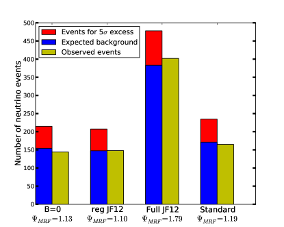
Figure 4: Distribution of expected background, observed events and discovery potential for different magnetic field hypothesis.

It is also relevant to mention the quantitative differences between the full JF12 and standard field models. In Tables 1 and 2, $E_{\nu}^{2}\Phi_{\nu}^{5\sigma}$ is smaller in the full JF12 by 15% and 17% respectively, indicating that the strength of the point source required for a $5\sigma$ discovery is somewhat overestimated in the case of the standard field.

Regarding the dependence of the power law index $\alpha$ on our results, we observe that the relative differences between the normalization constants for different field models are independent of $\alpha$. For the normalization constant itself we get higher values when $\alpha=2.3$. This can be explained by the steeply falling flux in this scheme, supressing contributions from the highest energy neutrinos at the tail, which have the largest effective area and are the most relevant for $\mu_{s}$. The values of $\mu_{s}^{5\sigma}$ remain almost intact after a change in $\alpha$, since the effect of this change is subdominant in our procedure. The results presented in Tables 1 and 2 are also shown in Figure 4, which is valid because of the negligible differences in $\Psi_{MRF}$ between both tables. The differences in the upper limits is justified by the deviations of the observed numbered of events with respect to its expected background. If we observe a large excess above the background, a larger flux per source consistent with the observed data are allowed. For this reason, in the full JF12 scenario, we have an upper limit $\sim 30\%$ higher than the other field models.

Finally, in Table 3 we explore the effects on $\mu_{s}^{5\sigma}$ due to variations of the JF12 field model parameters and compare them to the results of our parameterization, assuming an $E_{\nu}^{-2}$ signal flux and using the 72 TA event data sample. We chose the parameters $B_{0}$ and $\beta$, where $B_{0}$ represents the magnetic field strength of the random halo component and $\beta$ modulates the strength of the random striated component with respect to the regular component via the relation $B_{stri}^{2}=\beta B_{reg}^{2}$. There is an excellent agreement, of about 1%, between our parameterization and the JF12 numerical simulations, taking its best fit parameters. We achieve differences of at most $5\%$ after varying both parameters by one standard deviation.

V SUMMARY AND CONCLUSIONS

We have made a correlation analysis between the TA UHECR events and the IceCube-40 muon neutrino candidates under different GMF model assumptions. In particular, we have introduced the JF12 model, which expresses our best knowledge of the GMF. We have not found any correlations between the samples, regardless of the magnetic field hypothesis and the signal flux power law index, being the observed number of neutrino events consistent with the expected background. The JF12 full field model leads to a $90\%$ CL upper limit that is $\sim$ 30% higher compared to the other models.

We note that for the full JF12 field the angular bin size $\Psi_{MRF}$ is about 56% higher than the other models, which in turn requires a higher number of signal events $\mu_{s}^{5\sigma}$ to claim a $5\sigma$ discovery. In contrast to other assumptions of the magnetic deflection, the JF12 field model incorporates an energy and arrival direction dependence that improves the accuracy of the analysis. In doing so, these deflections are not overestimated and leads to a signal strength per source that is weaker by $\sim 20\%$ for a $5\sigma$ discovery. The latter observation gives us the hope that weaker sources can yield positive correlations given enough time. The relative differences between our results should stay the same for future measurements. This analysis hints towards positive correlations due to relaxed flux limits per source with further improvement of the knowledge of the GMF.

References

- (1) K. Greisen, Phys. Rev. Lett. 16, 748 (1966).
- (2) G.T. Zatsepin and V.A. Kuz’min, JETP Lett. 4, 78 (1966).
- (3) S. Adrián-Martínez et al. (ANTARES Collaboration), Astrophys. J. 774, 19 (2012).
- (4) K. Fang, T. Fujii, T. Linden and A. Olinto, Astrophys. J (to be published). [accepted for publication]
- (5) A. Keivani, G. Farrar and M. Sutherland, Astropart. Phys. 61, 47 (2015).
- (6) R. Jansson and G.R. Farrar, Astrophys. J. 757, 14 (2012).
- (7) R. Jansson and G.R. Farrar, Astrophys. J. 761, L11 (2012).
- (8) R.U. Abbasi et al. (Telescope Array Collaboration) Astrophys. J. 790, L21 (2014).
- (9) R. Abbasi et al. (IceCube Collaboration), Phys. Rev. D 84, 082001 (2011).
- (10) K. Dolag, D. Grasso, V. Springel and I. Tkachev, JETP Lett. 79, 583 (2004).
- Kotera & Lemoine (2008) K. Kotera and M. Lemoine, Phys. Rev. D 77, 123003 (2008).
- (12) R. Lauer et al. (IceCube Collaboration), Astrophys. Space Sci. Trans. 7, 201 (2011).
- (13) A. Aab et al. (Pierre Auger Collaboration), Eur. Phys. J. C 75, 269 (2015).
- (14) K.M. Górski et al., Astrophys. J. 622 758 (2005).
- (15) R. Alves Batista et al., in Proceedings of the 33rd International Cosmic Ray Conference, Rio de Janeiro, Brasil, 2013.
- (16) P. Abreu et al. (Pierre Auger Collaboration), Astropart. Phys. 34, 314 (2010).
- (17) M.G. Aartsen et al. (IceCube Collaboration), Phys. Rev. D, 89, 062007 (2014).
- (18) M.G. Aartsen et al. (IceCube Collaboration), Phys. Rev. Lett. 113 101101 (2014).
- (19) G.J. Feldman and R.D. Cousins, Phys. Rev. D, 57, 3873 (1998).