Topological septet pairing with spin-$\frac{3}{2}$ fermions – high partial-wave channel counterpart of the ³He-B phase

Abstract

We systematically generalize the exotic ³He-B phase, which not only exhibits unconventional symmetry but is also isotropic and topologically non-trivial, to arbitrary partial-wave channels with multi-component fermions. The concrete example with four-component fermions is illustrated including the isotropic $f$, $p$ and $d$-wave pairings in the spin septet, triplet, and quintet channels, respectively. The odd partial-wave channel pairings are topologically non-trivial, while pairings in even partial-wave channels are topologically trivial. The topological index reaches the largest value of $N^{2}$ in the $p$-wave channel ($N$ is half of the fermion component number). The surface spectra exhibit multiple linear and even high order Dirac cones. Applications to multi-orbital condensed matter systems and multi-component ultra-cold large spin fermion systems are discussed.

Superconductivity and paired superfluidity of neutral fermions possessing unconventional symmetries are among the central topics of condensed matter physics. If Cooper pairs formed by spin-$\frac{1}{2}$ fermions carry non-zero spin, their orbital symmetries are in the odd partial-wave channels. The $p$-wave paired superfluidity leggett1975 ; volovik2003 includes the ³He-A phase exhibiting point nodes anderson1961 , the fully gapped B phase balian1963 , and the recently reported polar state with linear nodes aoyama2006 ; dmitriev2015 . The $p$-wave superconductivity has also been extensively investigated in SrRu₂O₄ mackenzie2003 ; nelson2004 ; kidwingira2006 , and heavy fermion systems including UGe₂, URhGe, UCoGe aoki2012 . The $p$-wave superfluid ³He and superconductors exhibit rich topological structures of vortices and spin textures under rotations or in external magnetic fields, respectively scharnberg1980 ; salomaa1987 . In addition, experimental signatures of the possible nodal $f$-wave superconductivity have also been reported in UPt₃ machida2012 ; schemm2014 .

Among these unconventional pairing phases, the ³He-$B$ phase is distinct: in spite of its non-$s$-wave pairing symmetry and spin structure, the overall pairing structure remains isotropic and fully gapped. Its pairing exhibits the relative spin-orbit symmetry breaking from $SO_{L}(3)\otimes SO_{S}(3)$ to $SO_{J}(3)$ leggett1975 where $L$, $S$, and $J$ represent the orbital, spin, and total angular momentum, respectively. The relative spin-orbit symmetry-breaking has also been studied in the context of Pomeranchuk instability termed as unconventional magnetism leading to dynamic generation of spin-orbit coupling wu2004a ; wu2007 .

Furthermore, the ³He-$B$ phase possesses non-trivial topological properties kitaev2001 ; schnyder2008 ; ryu2010 . Topological states of matter have become a major research focus since the discovery of the integer quantum Hall effect klitzing1980 ; kohmoto1985 ; thouless1982 . Recently, the study of topological band structures has extended from time-reversal (TR) breaking systems to TR invariant systems kane2005 ; hasan2010 ; qi2011 , from two to three dimensions schnyder2008 ; moore2007 ; roy2010 , and from insulators to superconductors kitaev2001 ; schnyder2008 ; ryu2010 ; alicea2011 ; sau2010 ; lutchyn2010 ; qi2010 . The ³He-B phase is a 3D TR invariant topological Cooper pairing state. Its bulk Bogoliubov spectra are analogous to the 3D gapped Dirac fermions belonging to the DIII class characterized by an integer-valued index schnyder2008 . The non-trivial bulk topology gives rise to the gapless surface Dirac spectra of the mid-gap Andreev-Majorana modes chung2009 . Evidence of these low energy states has been reported in recent experiments bunkov2015 .

Because the electron Cooper pair can only be either spin singlet or triplet, the $p$-wave ³He-B phase looks the only choice of the unconventional 3D isotropic pairing state. In this article, we will show that actually there are much richer possibilities of this exotic class of pairing in all the partial-wave channels of $L\geq 1$. We consider multi-component fermions in both orbital-active solid state systems and ultra-cold atomic systems with large spin alkali and alkaline-earth fermions, both of which have recently attracted a great deal of attention wu2012 ; ho1999 ; wu2003 ; wu2006 ; deSalvo2010 ; gorshkov2010 ; taie2010 ; fang2015 ; fu2010 . For simplicity, below we introduce an effective spin $s$ to describe the multi-component fermion systems with the component number expressed as $2N=2s+1\geq 4$. Compared with the 2-component case, their Cooper pair spin structures are greatly enriched wu2010a ; ho1999 . For example, the 4-component spin-$\frac{3}{2}$ systems can support the $f$-wave septet, $p$-wave triplet, and $d$-wave quintet pairings, all of which are fully gapped and rotationally invariant. Nevertheless, only the odd partial-wave channel ones, i.e., the $p$ and $f$-wave pairings are topologically non-trivial. Their topological properties are analyzed both from calculating the bulk indices and surface Dirac cones of the Andreev-Majorana modes. For the $p$-wave case, the topological indices from all the helicity channels add up leading to a large value of $N^{2}$. Correspondingly the surface spectra exhibit the coexistence of 2D Dirac cones of all the orders from 1 to $2N-1$.

We begin with an $f$-wave spin septet Cooper pairing Hamiltonian in a 3D isotropic system of spin-$\frac{3}{2}$ fermions

$$H=\sum_{\vec{k}}\epsilon_{\vec{k}}c^{\dagger}_{\alpha}(\vec{k})c_{\alpha}(\vec{k})-\frac{g}{V_{0}}\sum_{\vec{k},\vec{k}^{\prime},m,\nu}P^{\dagger}_{m,\nu}(\vec{k})P_{m,\nu}(\vec{k}^{\prime}),$$ (1)

in which $\epsilon_{\vec{k}}=\frac{\hbar^{2}k^{2}}{2m}-\mu$ and $\mu$ is the chemical potential. $\alpha=\pm\frac{3}{2},\pm\frac{1}{2}$ is the spin index, $g$ is the pairing interaction strength, and $V_{0}$ is the system volume. The pairing operator is defined as $P^{\dagger}_{m,\nu}(\vec{k})=c^{\dagger}_{\alpha}(\vec{k})Y_{3m}(\hat{k})[S^{3\nu}R]_{\alpha\beta}c^{\dagger}_{\beta}(-\vec{k})$ where $\hat{k}=\vec{k}/k$, $Y_{3m}(\hat{k})$’s with $-3\leq m\leq 3$ are the 3rd order spherical harmonic functions, and $S^{3\nu}$ with $-3\leq\nu\leq 3$ are the rank-3 spherical tensors based on the spin operator $\vec{S}$ in the spin $\frac{3}{2}$-representation, where $\nu$ is the eigenvalue of $S_{z}$. For later convenience, $Y_{3m}(\hat{k})$ are normalized according to $\sum_{m}|Y_{3m}(\hat{k})|^{2}=1$. $R$ is the charge conjugation matrix defined as $R_{\alpha\beta}=(-)^{\alpha+\frac{1}{2}}\delta_{\alpha,-\beta}$ satisfying $R\vec{S}^{T}R^{-1}=-\vec{S}$ such that $R_{\alpha\beta}c^{\dagger}_{\beta}$ transforms in the same way under rotation as $c_{\alpha}$ does. The expressions for spherical harmonic functions and spin tensors are presented in Appendix A.

After the mean-field decomposition, Eq. 1 becomes

$$\frac{H_{MF}}{V}=\frac{1}{V}\sum^{\prime}_{\vec{k}}\Psi^{\dagger}(\vec{k})H(\vec{k})\Psi(\vec{k})+g\sum_{m,\nu}\Delta^{*}_{m,\nu}\Delta_{m,\nu},$$ (2)

in which $\vec{k}$ is summed over half of momentum space; $\Psi(\vec{k})=(c_{\vec{k},\alpha},c^{\dagger}_{-\vec{k},\alpha})^{T}$ is the Nambu spinor; the order parameter $\Delta_{m,\nu}$ is defined through the self-consistent equation as

$$\Delta_{m,\nu}=\frac{g}{V}\sum_{\vec{k}}\langle G|c_{\gamma}(-\vec{k})Y^{*}_{3m}(\vec{k})R^{\dagger}S^{3\nu,\dagger}c_{\delta}(\vec{k})|G\rangle$$ (3)

with $\langle G|...|G\rangle$ meaning the ground state average. The matrix kernel $H(\vec{k})$ in Eq. 2 is expressed as

$$H(\vec{k})=\epsilon(\vec{k})\tau_{3}\otimes I_{4\times 4}+\hat{\Delta}(\vec{k})\tau_{+}+\hat{\Delta}(-\vec{k})\tau_{-},$$ (4)

where $\tau_{3}$ and $\tau_{\pm}=\frac{1}{2}(\tau_{1}\pm i\tau_{2})$ are the Pauli matrices acting in the Nambu space. $\hat{\Delta}(\vec{k})$ is defined in the matrix form in spin space as

$$\hat{\Delta}(\vec{k})=\sum_{\nu}(S^{3\nu}R)d^{*,\nu}(\vec{k}),$$ (5)

where $d^{*,\nu}(\vec{k})=\Delta_{m,\nu}Y_{3m}(\hat{k})$ and is dubbed as the $d$-tensor in analogy to the $d$-vector in ³He. The usual $d$-vector is represented in its three Cartesian components, while here, the $d$-tensor is a rank-3 complex spherical tensor.

We consider the isotropic pairing with total angular momentum $J=0$, which is a generalization of the $p$-wave ³He-B phase. Similarly, it is fully gapped, and thus conceivably energetically favorable within the mean-field theory. Its $d^{\nu}(\vec{k})$ can be parametrized as $d^{\nu}(\vec{k})=c_{f}\Delta_{f}(\frac{k}{k_{f}})^{3}Y_{3\nu}(\hat{k})$, where $c_{f}$ is an overall normalization factor given in Appendix B. $\Delta_{f}$ is the complex gap magnitude, or, equivalently,

$$\hat{\Delta}(\vec{k})=\Delta_{f}(\frac{k}{k_{f}})^{3}K_{f}(\hat{k})R$$ (6)

in which $K_{f}=c_{f}U(\hat{k})S^{30}U^{\dagger}(\hat{k})$; $U(\hat{k})$ rotates the $z$-axis to $\hat{k}$ as defined in the following gauge $U(\hat{k})=e^{-i\phi_{k}s_{z}}e^{-i\theta_{k}s_{y}}$ in which $\theta_{k}$ and $\phi_{k}$ are polar and azimuthal angles of $\hat{k}$, respectively. The explicit form of $\hat{\Delta}(\hat{k})$ and the corresponding spontaneous symmetry breaking pattern are presented in Appendices B and C, respectively.

With the help of the helicity operator $h(\hat{k})=\hat{k}\cdot\vec{S}$, $K_{f}(\hat{k})$ can be further expressed in an explicitly rotational invariant form as

$$K_{f}(\hat{k})=-\frac{5}{2}h^{3}(\hat{k})+\frac{41}{8}h(\hat{k}),$$ (7)

which is diagonalized as $U^{\dagger}(\vec{k})K_{f}(\hat{k})U(\hat{k})=(-\frac{5}{2}S_{z}^{3}+\frac{41}{8}S_{z})$. For a helicity eigenstate with the eigenvalue $\lambda$, the corresponding eigenvalue $\xi_{\lambda}$ of $K_{f}(\hat{k})$ reads $\xi_{\lambda}=-\frac{3}{4},\frac{9}{4},-\frac{9}{4},\frac{3}{4}$ for $\lambda=\frac{3}{2},\frac{1}{2},-\frac{1}{2},-\frac{3}{2}$, respectively. The Bogoliubov quasi-particle spectra are $E_{\lambda}(\vec{k})=\sqrt{\epsilon^{2}(\vec{k})+|\Delta_{f}|^{2}(\frac{k}{k_{f}})^{6}\xi_{\lambda}^{2}}$ satisfying $E_{\lambda}(\vec{k})=E_{-\lambda}(\vec{k})$ due to the parity symmetry.

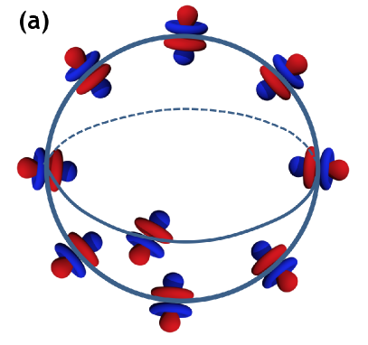
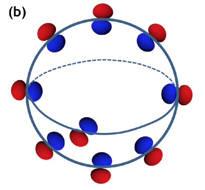
Figure 1: Pictorial representations of the pairing matrices over the Fermi surfaces of ($a$) the isotropic $f$-wave septet pairing and ($b$) the isotropic $p$-wave triplet pairing with spin-$\frac{3}{2}$ fermions. Intuitively, the $f$-wave matrix kernels $U(\hat{k})S^{30}U^{\dagger}(\hat{k})$ and the $p$-wave ones $U(\hat{k})S^{10}U^{\dagger}(\hat{k})$ for each wavevector $\vec{k}$ are depicted in their orbital counterpart harmonic functions in $(a)$ and $(b)$, respectively.

Next we study the pairing topological structure. The pairing Hamiltonian Eq. 4 in the Bogoliubov-de Gennes (B-deG) formalism possesses the particle-hole symmetry $C_{p}H(\vec{k})C_{p}^{-1}=-H^{*}(-\vec{k})$ with $C_{p}=\tau_{1}\otimes I_{4}$. Furthermore, the isotropic pairing state described by Eq. 6 is TR invariant satisfying $C_{T}H(\vec{k})C_{T}^{-1}=H^{*}(-\vec{k})$ with $C_{T}=I_{2}\otimes R$, and thus it belongs to the DIII class. The associated topological index is integer-valued which will be calculated following the method in Ref. [qi2010, ]. $H(\vec{k})$ is transformed with only two off-diagonal blocks as $\epsilon(\vec{k})\tau_{1}+\Delta_{f}(\frac{k}{k_{f}})^{3}K(\hat{k})\tau_{2}$. The singular-value-decomposition to its up-right block yields $U(\hat{k})L(k)\Lambda(k)U^{\dagger}(\hat{k})$, in which $L(k)$ and $\Lambda(k)$ are two diagonal matrices only dependent on the magnitude of $k$ defined as $L_{\lambda\lambda}(k)=E_{\lambda}(k)$ and $\Lambda_{\lambda\lambda}(k)=e^{i\theta_{\lambda}(k)}$, respectively. The angles satisfy $\tan\theta_{\lambda}(\vec{k})=-\frac{\Delta_{f}\xi_{\lambda}}{\epsilon_{\vec{k}}}(\frac{k}{k_{f}})^{3}$ and for simplicity $\Delta_{f}$ is set as positive. The $k^{3}$-dependence of the pairing amplitude is regularized: Beyond a cutoff $k_{c}$, $\Delta_{f}$ vanishes.

The topological index is calculated through the SU(4) matrix $Q_{\vec{k}}=U(\hat{k})\Lambda(k)U^{\dagger}(\hat{k})$ as

$$N_{w}=\frac{1}{24\pi^{2}}\int d^{3}{\vec{k}}\epsilon^{ijl}\mbox{Tr}[Q^{\dagger}_{\vec{k}}\partial_{i}Q_{\vec{k}}Q^{\dagger}_{\vec{k}}\partial_{j}Q_{\vec{k}}Q^{\dagger}_{\vec{k}}\partial_{l}Q_{\vec{k}}],$$ (8)

which is integer-valued characterizing the homotopic class of the mapping i.e., $\pi_{3}(SU(4))=\mathbb{Z}$. Nevertheless, $N_{w}$ is only well-defined up to a sign: After changing $\Delta_{f}\rightarrow-\Delta_{f}$, $N_{w}$ flips the sign. As shown in Appendix D, at $\mu>0$ $N_{w}$ is evaluated as

$$N_{w}=\sum_{\lambda=\pm\frac{3}{2},\pm\frac{1}{2}}\lambda\leavevmode\nobreak\ \mbox{sgn}(\xi_{\lambda}).$$ (9)

Its dependence on $\mbox{sgn}(\xi_{\lambda})$ is because $\theta_{\lambda}(\vec{k})$ varies from $0\rightarrow\frac{\pi}{2}\rightarrow\pi$ at $\xi_{\lambda}>0$ but from $\pi\rightarrow\frac{\pi}{2}\rightarrow 0$ as $k$ varies from $0$ to $k_{f}$ to $+\infty$. A similar form of Eq. 9 was obtained in Ref. [qi2010, ] in which the Fermi surface Chern number plays the role of $\lambda$ in Eq. 9. For two helicity pairs of $\lambda=\pm\frac{3}{2}$ and $\lambda=\pm\frac{1}{2}$, their contributions are with opposite signs, and thus $N_{w}=2$.

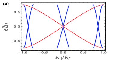
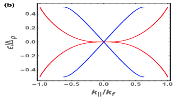
Figure 2: The gapless surface spectra for the isotropic $f$-wave septet pairing in ($a$) and for the isotropic $p$-wave triplet pairing in ($b$) with spin-$\frac{3}{2}$ fermions.

The non-trivial bulk topology gives rise to gapless surface Dirac cones. Because of the pairing isotropy, without loss of generality, an open planar boundary is chosen at $z=0$ with $\mu(z)=\epsilon_{f}>0$ at $z<0$ and $-\infty$ at $z>0$. The mean-field Hamiltonian becomes $H(\vec{k}_{\parallel},z)$ in which $\vec{k}_{\parallel}=(k_{x},k_{y})$ remains conserved while the translation symmetry along the $z$-axis is broken. The symmetry on the boundary is $C_{v\infty}$ including the uni-axial rotation around the $z$-axis and the reflection with respect to any vertical plane. $C_{v\infty}$ is also the little group symmetry at $\vec{k}_{\parallel}=0$, then the four zero Andreev-Majorana modes at $\vec{k}_{\parallel}=0$ are $s_{z}$ eigenstates denoted as $|0_{\alpha,f}\rangle$. The associated creation operators $\gamma^{\dagger}_{\alpha}$ are solved as

$$\gamma^{\dagger}_{\alpha}=\int^{0}_{-\infty}dz [ e^{i(\frac{\varphi}{2}+\frac{\pi}{4})}c^{\dagger}_{\alpha}(\vec{k}_{\parallel}=0,z)$$ (10)

$$+ e^{-i(\frac{\varphi}{2}+\frac{\pi}{4})}c_{-\alpha}(\vec{k}_{\parallel}=0,z)]u_{\alpha}(z),\ \ \,$$

where $\varphi$ is the phase of $\Delta$; $u_{f,\alpha}(z)$ is the zero mode wavefunction exponentially decaying along the $z$-axis, and its expression is presented in Appendix E.

The surface zero modes $|0_{\alpha,f}\rangle$ at $\vec{k}_{\parallel}=0$ possess an important property that the gapped bulk modes do not have: They are chiral eigen-modes satisfying $C_{ch}|0_{\alpha,f}\rangle=(-)^{\nu_{\alpha}}|0_{\alpha,f}\rangle$ with $\nu_{\alpha}=0$ for $\alpha=\frac{3}{2},-\frac{1}{2}$ and $\nu_{\alpha}=1$ for $\alpha=\frac{1}{2},-\frac{3}{2}$, respectively, in which the chiral operator is defined as $C_{ch}=iC_{p}C_{T}=i\tau_{1}\otimes R$. The mean-field Hamiltonian $H(\vec{k}_{\parallel},z)$ is in the DIII class satisfying the particle-hole and TR symmetries, and it transforms as $C_{ch}H(\vec{k}_{\parallel},z)C_{ch}^{-1}=-H(\vec{k}_{\parallel},z)$. Thus $C_{ch}$ is a symmetry only for zero modes. For a nonzero mode $|\psi_{n}\rangle$ and its chiral partner $|\psi_{\bar{n}}\rangle=C_{ch}|\psi_{n}\rangle$, their energies are opposite to each other, i.e., $\epsilon_{\bar{n}}=-\epsilon_{n}$. If a perturbation $\delta H$ remains in the DIII class, then $C_{ch}\delta HC_{ch}^{-1}=-\delta H$. $\delta H$ can only mix two zero modes with opposite chiral indices because $\langle 0_{\alpha,f}|\delta H|0_{\beta,f}\rangle=(-)^{\nu_{\alpha}+\nu_{\beta}+1}\langle 0_{\alpha,f}|\delta H|0_{\beta,f}\rangle$, and it is nonzero only if $\nu_{\alpha}\neq\nu_{\beta}$.

As moving away from $\vec{k}_{\parallel}=0$, the zero modes evolve to the midgap states developing energy dispersions. At $k_{\parallel}\ll k_{f}$, these midgap states can be solved by using the $k\cdot p$ perturbation theory within the subspace spanned by the zero modes $|0_{\alpha,f}\rangle$ at $\vec{k}_{\parallel}=0$. By setting $\delta H=H(\vec{k}_{\parallel},z)-H(0,z)$, the effective Hamiltonian to the linear order of $k_{\parallel}$ is

$$H_{mid}^{f}(\vec{k}_{\parallel})=\frac{9\Delta_{f}}{4k_{f}}\left(\begin{array}[]{cccc}0&-ik_{-}&0&O(k_{-}^{3})\\ ik_{+}&0&-2ik_{-}&0\\ 0&2ik_{+}&0&-ik_{-}\\ O(k_{+}^{3})&0&ik_{+}&0\end{array}\right),\ \ \,$$ (15)

where $k_{\pm}=k_{x}\pm ik_{y}$. The matrix elements in the same chiral sector are exactly zero, and the elements at the order of $O(k^{3}_{\pm})$ are neglected. The solutions consist two sets of 2D surface Dirac cone spectra represented by $E^{a(b)}_{\pm}(\vec{k}_{\parallel})=\pm v_{a(b)}k_{\parallel}$. The velocities are solved as $v_{a(b)}=\frac{9}{4}\frac{|\Delta_{f}|}{k_{f}}(\sqrt{2}\pm 1)$. We also develop a systematic method beyond the $k\cdot p$ theory to solve the midgap spectra for all the range of $k_{\parallel}$ as presented in Appendix H, and the results are plotted in Fig. 2 ($a$). In addition to the Dirac cones, there also exists an additional zero energy ring not captured by Eq. 15, which is located at $k/k_{f}=\frac{\sqrt{3}}{2}$ as analyzed in Appendix E.

Now we move to other unconventional isotropic pairings of spin-$\frac{3}{2}$ fermions in the $p$ and $d$-wave channels. The $p$-wave triplet one is topologically non-trivial, and the analysis can be performed in the same way as above. The pairing matrix is $\hat{\Delta}_{p}(\vec{k})=\sum_{\nu=0,\pm 1}(S^{1\nu}R)d_{p}^{*,\nu}(\vec{k})=\Delta_{p}\frac{k}{k_{f}}K_{p}(\hat{k})R,$ where $S^{1\nu}$ is the rank-1 spin tensor, $d_{p}^{\nu}=\Delta_{p}(\frac{k}{k_{f}})Y_{1\nu}(\hat{k})$, and $K_{p}(\hat{k})=\hat{k}\cdot\vec{S}$ is just the helicity operator. The quasi-particle spectra are fully gapped as $E_{\lambda}(\vec{k})=\sqrt{\epsilon^{2}(\vec{k})+|\Delta_{p}|^{2}(\frac{k}{k_{f}})^{2}\lambda^{2}}$, and the topological index of this pairing can be evaluated based on Eq. 9 by replacing the eigenvalues of $K_{f}(\hat{k})$ with those of $K_{p}(\hat{k})$. The contributions from two helicity pairs of $\lambda=\pm\frac{3}{2}$ and $\pm\frac{1}{2}$ add up leading to a high value $N_{w}=4$. In comparison, the topological index of the ³He-B phase is only 1, and thus their topological sectors are different in spite of the same pairing symmetry.

The surface spectra of the isotropic $p$-wave pairing with spin-$\frac{3}{2}$ fermions are interesting: They exhibit a cubic Dirac cone in addition to a linear one. Consider the same planar boundary configuration as before, similarly for each spin component $\alpha$ there exists one zero mode at $\vec{k}_{\parallel}=0$ labeled by $|0_{\alpha,p}\rangle$. Again we perform the $k\cdot p$ analysis at $k_{\parallel}\ll k_{f}$ in the subspace spanned by $|0_{\alpha,p}\rangle$ with respect to $\delta H=H(\vec{k}_{\parallel},z)-H(0,z)$. The chiral eigenvalue of $|0_{\alpha,p}\rangle$ is $(-)^{\nu_{\alpha}}=\mbox{sgn}(\alpha)$, which leads to a different structure of effective Hamiltonian from that of the $f$-wave one. Only $|0_{\pm\frac{1}{2},p}\rangle$ can be directly coupled by $\delta H$, which leads to a linear Dirac cone. In contrast, the pair of states $|0_{\pm\frac{3}{2},p}\rangle$ are not directly coupled, rather $|0_{\frac{3}{2},p}\rangle$ and $|0_{-\frac{1}{2},p}\rangle$ are coupled through the 2nd order perturbation theory, and so do $|0_{-\frac{3}{2},p}\rangle$ and $|0_{\frac{1}{2},p}\rangle$. Consequently, $|0_{\pm\frac{3}{2},p}\rangle$ are coupled at the order of $(\delta H)^{3}$ developing a cubic Dirac cone as shown in Appendix F. The above analysis is confirmed by the solution based on the non-perturbative method in Appendix H, as plotted in Fig. 2 (b).

In contrast, the $d$-wave spin quintet isotropic pairing of spin-$\frac{3}{2}$ fermions are topologically trivial. By imitating the analyses above, we replace $K_{f}(\hat{k})$ with $K_{d}(\hat{k})=2(\hat{k}\cdot\vec{S})^{2}-\frac{5}{2}I_{4}$. Different from the kernels $K_{p}$ and $K_{f}$ in odd partial-wave channels, $K_{d}$’s eigenvalues are even with respect to the helicity index, i.e., $\xi^{d}_{\lambda}=\xi^{d}_{-\lambda}$, such that $N_{w}$ vanishes. This result agrees with that 3D TR invariant topological superconductors should be parity odd as shown in Ref. [zhangfan2013, ]. The explicit calculation of the surface spectra in Appendix G confirms this point showing the absence of zero modes.

The above analysis can be straightforwardly applied to multi-component fermion systems with a general spin value $s=N-\frac{1}{2}$. The spin-tensors at the order of $l$ are denoted as $S^{lm}$ with $0\leq l\leq 2S$ and $-l\leq m\leq l$. For each partial-wave channel $0\leq l\leq 2S$, there exists an isotropic pairing with the pairing matrix $\hat{\Delta}(\hat{k})=\Delta_{l}(\frac{k}{k_{f}})^{l}K_{l}(\hat{k})R$ in which $K_{l}=U(\hat{k})S^{l0}U^{\dagger}(\hat{k})$, whose topological index $N_{w}(l)$ is determined by the sign pattern of the elements of the diagonal matrix $S^{l0}$. For even and odd values of $l$, $S^{l0}_{\alpha\alpha}=\pm S^{l0}_{-\alpha-\alpha}$, respectively, and thus $N_{w}^{l}$ vanishes when $l$ is even, while for odd values of $l$,

$$N_{w}(l)=\sum_{\lambda>0}2\lambda\leavevmode\nobreak\ \mbox{sgn}(S^{l0}_{\lambda\lambda}),$$ (16)

in which $S^{l0}_{\alpha\alpha}=(-)^{\alpha+\frac{1}{2}}\langle S\alpha,S-\alpha|SS;l0\rangle$ up to an overall factor. The largest value of $N_{w}$ is reached for the $p$-wave case: Since $S^{10}\propto S_{z}$, contributions from all the components add together leading to $N_{w}=N^{2}$. The ³He-B phase of spin-$\frac{1}{2}$ fermions and the isotropic $p$-wave pairing with spin-$\frac{3}{2}$ fermions are two examples. As for the surface zero modes $|0_{\alpha,p}\rangle$ at $\vec{k}_{\parallel}=0$, their chiral indices equal $\mbox{sgn}(\alpha)$. As a result, similar to the spin-$\frac{3}{2}$ case, when performing the $k\cdot p$ analysis for midgap states within the subspace spanned by $|0_{\alpha,p}\rangle$, only $|0_{\pm\frac{1}{2},p}\rangle$ are directly coupled leading to a linear Dirac cone, and other pairs of $|0_{\pm\alpha,p}\rangle$ are indirectly coupled at the order of $(\delta H)^{2\alpha}$ leading to high order Dirac cones.

Multi-component fermion systems are not rare in nature. In solid state systems, many materials are orbital-active including semiconductors, transition metal oxides, and heavy fermion systems. Due to spin-orbit coupling, their band structures are denoted by electron total angular momentum $j$ and in many situations $j>\frac{1}{2}$. For example, in the hole-doped semiconductors, the valence band carries $j=\frac{3}{2}$ as described by the Luttinger model winkler2003 . Superconductivity has been discovered in these systems including hole-doped diamond and Germanium takano2004 ; ekimov2004 ; herrmannsdorfer2009 . Although in these materials, the Cooper pairings are mostly of the conventional $s$-wave symmetry arising from the electron-phonon interaction, it is natural to further consider unconventional pairing states in systems with similar band structures but stronger correlation effects. The $p$-wave pairing based on the Luttinger model has been studied in Ref. [fang2015, ]. In ultra-cold atom systems, many alkali and alkaline-earth fermions often carry large hyperfine spin values $F>\frac{1}{2}$, and thus their Cooper pair spin structures are enriched taking values from $0$ to $2F$ not just singlet and triplet as in the spin-$\frac{1}{2}$ case ho1999 ; wu2006 ; wu2010a .

In multi-component solid state systems, there often exists spin-orbit coupling. For example, the Luttinger model describing hole-doped semi-conductors winkler2003 , contains an isotropic spin-orbit coupling $H_{so}=\gamma_{2}k^{2}(\hat{k}\cdot\vec{S})^{2}$. Since $H_{so}$ is diagonalized in the helicity eigenbasis, we only need to update the kinetic energy with $\epsilon_{k\lambda}=\epsilon_{k}+\gamma k^{2}\lambda^{2}$ in the mean-field analysis, which satisfies $\epsilon_{k\lambda}=\epsilon_{k,-\lambda}$, and the pairing structure described by Eq. 6 is not affected. The topological properties are the same as analyzed before because the index formula Eq. 9 remains valid and the surface mid-gap state calculation can be performed qualitatively similarly. Nevertheless, the symmetry breaking pattern is changed. The relative spin-orbit symmetry is already explicitly broken by the $H_{so}$. The spin-orbit coupled Goldstone modes in ³He-B become gapped pseudo-Goldstone modes with the gap proportional to the spin-orbit coupling strength $\gamma_{2}$.

In summary, we have found that multi-component fermion systems can support a class of exotic isotropic pairing states analogous to the ³He-B phase with unconventional pairing symmetries and non-trivial topological structures. High-rank spin tensors are entangled with orbital partial-waves at the same order to form isotropic gap functions. For the spin-$\frac{3}{2}$ case, the odd partial-wave channel pairings carry topological indices 2 and 4 for the $f$ and $p$-wave pairings, respectively, while the $d$-wave channel pairing is topologically trivial. The surface Dirac cones of mid-gap modes are solved analytically which exhibit two linear Dirac cones in the $f$-wave case, and the coexistence of linear and cubic Dirac cones in the $p$-wave case. Generalizations to systems with even more fermion components can be performed straightforwardly. This work provides an important guidance to search for novel non-trivial topological pairing states in both condensed matter and ultra-cold atom systems.

Acknowledgments W. Y. and C. W. are supported by the NSF DMR-1410375 and AFOSR FA9550-14-1-0168. Y. L. is grateful for the support from the Princeton Center for Theoretical Science. C. W. acknowledges the supports from the National Natural Science Foundation of China (11328403), the CAS/SAFEA International Partnership Program for Creative Research Teams of China, and the President’s Research Catalyst Awards CA-15-327861 from the University of California Office of the President.

Note added. After the submission of this manuscript, the evidence for the septet pairing with spin-$\frac{3}{2}$ fermions has been reported in the rare earth-based half-Heusler superconductors kim2016 .

Appendix A Spherical harmonic functions and high-rank Spin tensor operators

In this section, we present spherical harmonic functions in momentum space and high-rank spin tensors.

For convenience in the main text, we normalize the spherical harmonic functions $Y_{lm}(\hat{k})$ defined on the Fermi surface satisfying

$$\sum_{m=-l}^{l}|Y_{lm}(\hat{k})|^{2}=1.$$ (17)

This normalization differs from the usual one of $\int d\Omega_{k}|Y_{lm}(\hat{k})|^{2}=1$ only by an overall factor $\sqrt{\frac{4\pi}{2l+1}}$. More explicitly, for the $p$-wave case, they are defined as

$$kY_{1\pm 1}(\hat{k}) = \mp\frac{1}{\sqrt{2}}k_{\pm},\ \ \,\ \ \,kY_{10}(\hat{k})=k_{z},$$ (18)

For the $d$-wave case, they are defined as

$$k^{2}Y_{2\pm 2}(\hat{k}) = \sqrt{\frac{3}{8}}k_{\pm}^{2},\ \ \,\ \ \,k^{2}Y_{2\pm 1}(\hat{k})=\mp\sqrt{\frac{3}{2}}k_{\pm}k_{z},$$

$$k^{2}Y_{20}(\hat{k}) = \frac{1}{2}(3k_{z}^{2}-k^{2}).$$ (19)

For the $f$-wave case, they are defined as

$$k^{3}Y_{3\pm 3}(\hat{k}) = \mp\frac{\sqrt{5}}{4}k_{\pm}^{3},\ \ \,\ \ \,k^{3}Y_{3\pm 2}(\hat{k})=\frac{\sqrt{30}}{4}k_{\pm}^{2}k_{z},$$

$$k^{3}Y_{3\pm 1}(\hat{k}) = \pm\frac{\sqrt{3}}{4}k_{\pm}(k^{2}-5k_{z}^{2}),$$

$$k^{3}Y_{30}(\hat{k}) = -\frac{1}{2}(3k^{2}-5k_{z}^{2})k_{z}.$$ (20)

All of them are homogeneous polynomials of momentum components $k_{x}$, $k_{y}$ and $k_{z}$.

The spin-$\frac{3}{2}$ matrices are defined in the standard way as

$$S_{+} = \left(\begin{array}[]{cccc}0&\sqrt{3}&0&0\\ 0&0&2&0\\ 0&0&0&\sqrt{3}\\ 0&0&0&0\end{array}\right),$$ (25)

$$S_{-} = S_{+}^{\dagger},$$

$$S_{z} = \left(\begin{array}[]{cccc}\frac{3}{2}&0&0&0\\ 0&\frac{1}{2}&0&0\\ 0&0&-\frac{1}{2}&0\\ 0&0&0&-\frac{3}{2}\end{array}\right),$$ (30)

in which $S_{\pm}=S_{x}\pm iS_{y}$. The general rank-$k$ spin tensors $S_{jm}$ satisfy

$$[S_{-},S_{jm}] = \sqrt{(j+m)(j-m+1)}S_{jm-1}.$$ (31)

Based on these relations, we can build up spin tensors. For example, the rank-1 tensors are defined as

$$S_{11}=-\frac{1}{\sqrt{2}}S_{+},\ \ \,S_{10}=S_{z},\ \ \,S_{1-1}=\frac{1}{\sqrt{2}}S_{-}.$$ (32)

The rank-2 tensors are spin quadrupole operators defined as

$$S_{22} = \frac{1}{\sqrt{3}}S_{11}^{2}=\left(\begin{array}[]{cccc}0&0&1&0\\ 0&0&0&1\\ 0&0&0&0\\ 0&0&0&0\end{array}\right)$$ (37)

$$S_{21} = \frac{1}{2}[S_{-},S_{22}]=\left(\begin{array}[]{cccc}0&-1&0&0\\ 0&0&0&0\\ 0&0&0&1\\ 0&0&0&0\end{array}\right)$$ (42)

$$S_{20} = \frac{1}{\sqrt{6}}[S_{-},S_{21}]=\frac{1}{\sqrt{2}}\left(\begin{array}[]{cccc}1&0&0&0\\ 0&-1&0&0\\ 0&0&-1&0\\ 0&0&0&1\end{array}\right)$$ (47)

$$S_{2-1} = \frac{1}{\sqrt{6}}[S_{-},S_{20}]=-S_{21}^{\dagger}$$

$$S_{2-2} = \frac{1}{2}[S_{-},S_{2-1}]=S_{22}^{\dagger}.$$ (48)

This set of tensors can be organized into the Dirac $\Gamma$ matrices through the relations of

$$\Gamma_{1} = -i(S_{22}-S_{2-2}),\ \ \,\Gamma_{5}=S_{22}+S_{2-2}$$

$$\Gamma_{2} = -S_{21}+S_{2-1},\ \ \,\Gamma_{3}=i(S_{21}+S_{2-1})$$

$$\Gamma_{4} = \sqrt{2}S_{20},$$ (49)

which satisfy the anti-commutation relation

$$\Gamma^{a}\Gamma^{b}+\Gamma^{b}\Gamma^{a}=2\delta_{ab}.$$ (50)

The rank-3 spin tensors $S_{3,m}$, also called spin-octupole operators, are constructed as follows

$$S_{33} = \frac{\sqrt{2}}{3}S_{11}^{3}=-\left(\begin{array}[]{cccc}0&0&0&1\\ 0&0&0&0\\ 0&0&0&0\\ 0&0&0&0\end{array}\right),\hskip 71.13188ptS_{32}=\frac{1}{\sqrt{6}}[S_{-},S_{33}]=\frac{\sqrt{2}}{2}\left(\begin{array}[]{cccc}0&0&1&0\\ 0&0&0&-1\\ 0&0&0&0\\ 0&0&0&0\end{array}\right),$$ (59)

$$S_{31} = \frac{1}{\sqrt{10}}[S_{-},S_{32}]=-\frac{1}{\sqrt{5}}\left(\begin{array}[]{cccc}0&1&0&0\\ 0&0&-\sqrt{3}&0\\ 0&0&0&1\\ 0&0&0&0\end{array}\right),\ \ \,S_{30}=\frac{1}{2\sqrt{3}}[S_{-},S_{31}]=\frac{1}{2\sqrt{5}}\left(\begin{array}[]{cccc}1&0&0&0\\ 0&-3&0&0\\ 0&0&3&0\\ 0&0&0&-1\end{array}\right),$$ (68)

$$S_{3,-1} = \frac{1}{2\sqrt{3}}[S_{-},S_{30}]=-S_{31}^{\dagger},\hskip 91.04881ptS_{3,-2}=\frac{1}{\sqrt{10}}[S_{-},S_{3,-1}]=S_{32},$$

$$S_{3,-3} = \frac{1}{\sqrt{6}}[S_{-},S_{3,-2}]=-S_{33}^{\dagger}$$ (69)

Appendix B Pairing matrices for the isotropic $p$, $d$, and $f$-wave

By using the spherical harmonic functions $Y_{lm}(\hat{k})$ and spin-tensors, we can construct the pairing matrices for the isotropic pairings for the spin-$\frac{3}{2}$ fermions in the $p$, $d$, and $f$-wave channels, respectively. The pairing matrix $\Delta_{\alpha\beta}(\vec{k})$ in momentum space can be represented as

$$\Delta^{l}_{\alpha\beta}(\vec{k}) = c_{l}\Delta\left(\frac{k}{k_{f}}\right)^{l}(-)^{m}Y_{lm}(\hat{k})S^{lm}R$$ (70)

$$= c_{l}\Delta\left(\frac{k}{k_{f}}\right)^{l}Y_{lm}^{*}(\hat{k})S^{lm}R,$$

in which $l=1,2,3$ represent $p$, $d$, and $f$-wave pairings, respectively, while $c_{l}$ is an overall constant factor. These pairing structures are isotropic in analogy to the ³He-B phase: the pairing orbital angular momenta are $l$, and the pairing spins are also $l$, such that they add together into the channel of total angular momentum $J=0$. The matrix kernel $Y_{lm}^{*}(\hat{k})S^{lm}$ can be explicitly represented in isotropic forms as

$$Y_{lm}^{*}(\hat{k})S^{lm}=\left\{\begin{array}[]{ll}\vec{k}\cdot\vec{S},&(l=1)\\ \frac{1}{\sqrt{2}}(\vec{k}\cdot\vec{S})^{2}-\frac{5}{4\sqrt{2}}k^{2},&(l=2)\\ \frac{\sqrt{5}}{3}(\vec{k}\cdot\vec{S})^{3}-\frac{41}{12\sqrt{5}}k^{2}(\vec{k}\cdot\vec{S}),&(l=3)\end{array}\right.$$ (74)

More explicitly, the pairing matrix in momentum space can be expressed as follows. In the $p$-wave case ($c_{1}=1$), it is

$$\Delta^{p}_{\alpha\beta}(\vec{k})=\frac{\Delta}{k_{f}}\left(\begin{array}[]{cccc}0&0&-\frac{\sqrt{3}}{2}k_{-}&\frac{3}{2}k_{z}\\ 0&k_{-}&-\frac{1}{2}k_{z}&\frac{\sqrt{3}}{2}k_{+}\\ -\frac{\sqrt{3}}{2}k_{-}&-\frac{1}{2}k_{z}&-k_{+}&0\\ \frac{3}{2}k_{z}&\frac{\sqrt{3}}{2}k_{+}&0&0\end{array}\right).$$ (80)

In the $d$-wave case ($c_{2}=2\sqrt{2}$), it reads

$$\Delta^{d}_{\alpha\beta}(\vec{k})=\frac{\Delta}{k_{f}^{2}}\left(\begin{array}[]{cccc}0&\sqrt{3}k_{-}^{2}&-2\sqrt{3}k_{-}k_{z}&3k_{z}^{2}-k^{2}\\ -\sqrt{3}k_{-}^{2}&0&3k_{z}^{2}-k^{2}&2\sqrt{3}k_{+}k_{z}\\ 2\sqrt{3}k_{-}k_{z}&k^{2}-3k_{z}^{2}&0&\sqrt{3}k_{+}^{2}\\ k^{2}-3k_{z}^{2}&-2\sqrt{3}k_{+}k_{z}&-\sqrt{3}k_{+}^{2}&0\end{array}\right),$$ (86)

and in the $f$-wave case ($c_{3}=-\frac{3\sqrt{5}}{2}$), it becomes

$$\Delta_{\alpha\beta}(\vec{k})=\frac{3\sqrt{3}\Delta}{8k_{f}^{3}}\left(\begin{array}[]{cccc}\frac{5}{\sqrt{3}}k_{-}^{3}&-5k_{-}^{2}k_{z}&-k_{-}(k^{2}-5k_{z}^{2})&\frac{1}{\sqrt{3}}(3k^{2}-5k_{z}^{2})k_{z}\\ -5k_{-}^{2}k_{z}&-\sqrt{3}k_{-}(k^{2}-5k_{z}^{2})&\sqrt{3}(3k^{2}-5k_{z}^{2})k_{z}&k_{+}(k^{2}-5k_{z}^{2})\\ -k_{-}(k^{2}-5k_{z}^{2})&\sqrt{3}(3k^{2}-5k_{z}^{2})k_{z}&\sqrt{3}k_{+}(k^{2}-5k_{z}^{2})&-5k_{+}^{2}k_{z}\\ \frac{1}{\sqrt{3}}(3k^{2}-5k_{z}^{2})k_{z}&k_{+}(k^{2}-5k_{z}^{2})&-5k_{+}^{2}k_{z}&-\frac{5}{\sqrt{3}}k_{+}^{3}\end{array}\right).$$ (91)

The general mean-field Hamiltonian in coordinate space is represented as

$$H=\frac{1}{2}\int d^{3}\vec{r}\Psi^{\dagger}(\vec{r}) \left[\begin{array}[]{cc}(-\frac{\hbar^{2}}{2m}\nabla^{2}-\mu)I_{4}&c_{l}\frac{\Delta}{k_{f}^{l}}Y^{*}_{lm}(-i\nabla)S^{lm}R\\ c_{l}\frac{\Delta}{k_{f}^{l}}(Y^{*}_{lm}(-i\nabla)S^{lm}R)^{\dagger}&-(-\frac{\hbar^{2}}{2m}\nabla^{2}-\mu)I_{4}\end{array}\right]\Psi(\vec{r}),$$ (94)

in which $\Psi^{\dagger}(\vec{r})=(c^{\dagger}_{\alpha}(\vec{r}),c_{\beta}(\vec{r}))$ is the Nambu spinor; $-i\nabla$ replaces $\vec{k}$ in the expressions of $k^{l}Y_{lm}(\vec{k})$.

Appendix C The symmetry properties

Here we use the isotropic $f$-wave pairing state as an example to illustrate the symmetry properties of this class of pairings. The Hamiltonian Eq. 1 (main text) processes both rotation symmetries in the orbital and spin channels, i.e., $SO_{L}(3)\times SO_{S}(3)$, while in the isotropic pairing state characterized by Eq. 5 (main text) only the total angular momentum is conserved, i.e., the residue symmetry is $SO_{J}(3)$. The general configuration of the $d$-tensor can be expressed as

$$d_{R}^{\nu}(\hat{k})=d^{\nu}(R^{-1}\hat{k})=D^{l=3}_{\nu\nu^{\prime}}(R)d^{\nu^{\prime}}(\hat{k}),$$ (95)

where $R$ is an arbitrary SO(3) rotation and $D^{l}_{\nu\nu\prime}(R)$ is the rotation $D$-matrix. The relative SO symmetry is spontaneously broken similar to the case of ³He-B, and here it is realized in a high representation of angular momentum. Combining with the $U(1)$ gauge symmetry breaking in the paired superfluid state, the Goldstone manifold is $[SO_{L}(3)\otimes SO_{S}(3)\otimes U(1)]/SO_{J}(3)=SO(3)\otimes U(1)$. Accordingly there exist four branches of Goldstone modes, including one branch of phonon mode and three branches of relative spin-orbit modes.

Appendix D Calculation of the bulk topological index

In this section, we calculate the topological index of various pairing states. According to the definition of $Q(\vec{k})=U^{\dagger}(\hat{k})\Lambda(k)U(\hat{k})$ in which $U$ and $U^{\dagger}$ only depend on the direction of $\vec{k}$, while $\Lambda(k)$ only depends on the magnitude of $k$, we have

$$\nabla_{k}Q = U^{\dagger}\nabla_{k}\Lambda(k)U,$$

$$\nabla_{\theta}Q = \nabla_{\theta}U^{\dagger}\Lambda U+U^{\dagger}\Lambda\nabla_{\theta}U,$$

$$\nabla_{\phi}Q = \nabla_{\phi}U^{\dagger}\Lambda U+U^{\dagger}\Lambda\nabla_{\phi}U,$$ (96)

in which $\nabla_{k}=\hat{k}\cdot\nabla$, $\nabla_{\theta}=\hat{e}_{\theta_{k}}\cdot\nabla$, $\nabla_{\phi}=\hat{e}_{\phi_{k}}\cdot\nabla$. Substituting the above equations into Eq. 8 in the main text, after simplification, we arrive at

$$N_{w} = \frac{1}{4\pi^{2}}\int d^{3}\vec{k}\mbox{Tr}(\nabla_{\theta}U\nabla_{\phi}U^{\dagger}-\nabla_{\phi}U\nabla_{\theta}U^{\dagger})\nabla_{k}\Lambda\Lambda^{\dagger},$$ (97)

$$= \sum_{\lambda}q_{\lambda}w_{\lambda},$$

in which $q_{\lambda}$ is the monopole charge associated to the Berry curvature of the helicity eigenstate; the corresponding eigenvalue $\lambda$ is defined as

$$q_{\lambda} = \int\frac{k^{2}d\Omega_{k}}{4\pi}F^{\lambda}_{\theta\phi}(\hat{k})$$ (98)

$$= \int\frac{k^{2}d\Omega_{k}}{4\pi}(-i)\left(\nabla_{\theta}U\nabla_{\phi}U^{\dagger}-\nabla_{\phi}U\nabla_{\theta}U^{\dagger}\right)_{\lambda\lambda}$$

$$= \lambda,$$

and $w_{\lambda}$ is the winding number of the angular $\theta_{\lambda}(k)$ along the radial direction of $k$ as

$$w_{\lambda}=\int_{0}^{+\infty}\frac{dk}{\pi}\leavevmode\nobreak\ \left(i\nabla\Lambda\Lambda^{\dagger}\right)_{\lambda\lambda}=\left\{\begin{array}[]{l}\mbox{sgn}(\xi_{\lambda})\leavevmode\nobreak\ \leavevmode\nobreak\ (\mu>0),\\ 0\leavevmode\nobreak\ \leavevmode\nobreak\ (\mu<0).\\ \end{array}\right.$$ (101)

Consequently, we arrive at

$$N_{w}=\left\{\begin{array}[]{l}\sum_{\lambda}\lambda\leavevmode\nobreak\ \mbox{sgn}(\xi_{\lambda})\leavevmode\nobreak\ \leavevmode\nobreak\ (\mu>0),\\ 0\leavevmode\nobreak\ \leavevmode\nobreak\ (\mu<0).\end{array}\right.$$ (105)

Appendix E The surface modes of the $f$-wave isotropic pairing

In this part, we study the gapless surface states of the $f$-wave septet pairing.

We study a boundary imposed at $z=0$ with a spatial dependent chemical potential $\mu(z)$: $\mu_{L}=\frac{\hbar k_{f}^{2}}{2m}>0$ at $z<0$ and $\mu_{R}<0$ at $z>0$. For simplicity, we consider the case of $|\mu_{R}|\gg\mu_{L}$ and finally take the limit of $|\mu_{R}|\rightarrow\infty$, i.e., at $z>0$ is the vacuum.

E.1 The $f$-wave zero modes at $\vec{k}_{\parallel}=0$

To warm up, we first consider the case of $\vec{k}_{\parallel}=0$ in which $S_{z}$ remains a good quantum number, and the zero modes described by different $S_{z}$ eigenvalues decouple. The B-deG equation of the zero mode with $S_{z}$-eigenvalue $\alpha$ becomes

$$\left(\begin{array}[]{cc}-\frac{\hbar^{2}}{2m}\frac{d^{2}}{dz^{2}}-\mu(z)&-i\frac{\Delta_{\alpha}}{k_{f}^{3}}\frac{d^{3}}{dz^{3}}\\ -i\frac{\Delta_{\alpha}}{k_{f}^{3}}\frac{d^{3}}{dz^{3}}&\frac{\hbar^{2}}{2m}\frac{d^{2}}{dz^{2}}+\mu(z)\end{array}\right)\left(\begin{array}[]{c}u^{0}_{\alpha}(z)\\ v^{0}_{-\alpha}(z)\end{array}\right)=0,$$ (110)

in which $\Delta_{\pm\frac{3}{2}}=\frac{3}{4}\Delta$ and $\Delta_{\pm\frac{1}{2}}=\frac{9}{4}\Delta$. The boundary condition is that

$$u_{0}(z)\rightarrow 0,\ \ \,v_{0}(z)\rightarrow 0,$$ (112)

as $z\rightarrow\pm\infty$.

Eq. 10 (main text) is invariant under the operation of $\left(\begin{array}[]{c}u_{0}\\ v_{0}\end{array}\right)\rightarrow i\tau_{2}\left(\begin{array}[]{c}u_{0}\\ v_{0}\end{array}\right)$ in which $\tau_{2}$ acts in the Nambu space, thus we can set $v_{0}=\pm iu_{0}$. As it will be clear later that the solution actually satisfies $v_{0}(z)=-iu_{0}(z)$, the other one with $v_{0}(z)=iu_{0}(z)$ corresponds to the case that the system lies at $z>0$ and the vacuum is at $z<0$. Then the equation becomes

$$\left(-\frac{\hbar^{2}}{2m}\frac{d^{2}}{dz^{2}}-\mu(z)-\frac{\Delta_{\alpha}}{k_{f}^{3}}\frac{d^{3}}{dz^{3}}\right)u_{0}(z)=0.$$ (113)

We try the solution $u_{0}(z)\sim e^{\beta_{L}z}$ at $z<0$, and, $e^{\beta_{R}z}$ at $z>0$, and thus $\rm{Re}\beta_{L}>0$ and $\rm{Re}\beta_{R}<0$, respectively.

At $z<0$, $\beta_{L}$ satisfies the cubic equation with real coefficients

$$\left(\frac{\beta_{L}}{k_{f}}\right)^{3}+\frac{\epsilon_{f}}{\Delta_{\alpha}}\left(\frac{\beta_{L}}{k_{f}}\right)^{2}+\frac{\epsilon_{f}}{\Delta_{\alpha}}=0,$$ (114)

which has a pair of conjugate complex roots and one real root. We only consider the weak pairing limit that $\frac{\Delta}{\epsilon_{f}}\ll 1$. The solutions correct to the linear order of $\frac{\Delta}{\epsilon_{f}}\ll 1$ are

$$\left(\frac{\beta_{L}}{k_{f}}\right)_{1,2}\approx\pm i+\frac{\Delta_{\alpha}}{2\epsilon_{f}},\ \ \,\left(\frac{\beta_{L}}{k_{f}}\right)_{3}\approx-\frac{\epsilon_{f}}{\Delta_{\alpha}},$$ (115)

and thus only $(\frac{\beta_{L}}{k_{f}})_{1,2}$ can be kept. Similarly, at $z>0$, in the case of $|\mu_{R}|\gg\epsilon_{f}$, there exists a pair of complex conjugate roots and one real root for $\beta_{R}$ as

$$\left(\frac{\beta_{R}}{k_{f}}\right)_{1,2}\approx c\left(-\frac{1}{2}\pm i\frac{\sqrt{3}}{2}\right),\ \ \,(\frac{\beta_{R}}{k_{f}})_{3}\approx c,$$ (116)

in which $c=\left(|\mu_{R}|/\Delta_{\alpha}\right)^{\frac{1}{3}}$.

Because Eq. 10 (main text) is a 3rd order differential equation, all of $u_{0}(z),\frac{d}{dz}u_{0}(z),\frac{d^{2}}{dz^{2}}u_{0}(z)$ need to be continuous at the boundary $z=0$. For this purpose, we construct the following solution

$$u_{0}(z)=\left\{\begin{array}[]{cc}A_{L}\sin(k_{f}z+\phi_{L})e^{\frac{\Delta_{\alpha}}{2\epsilon_{f}}k_{f}z}&(z<0)\\ A_{R}\sin(\frac{\sqrt{3}}{2}ck_{f}z+\phi_{R})e^{-\frac{c}{2}k_{f}z}&(z>0)\end{array}\right.,\ \ \,$$ (119)

in which the four parameters $A_{L(R)}$ and $\phi_{L(R)}$ are sufficient to match three continuous conditions. In the case of $c\rightarrow+\infty$, the results can be simplified as

$$\phi_{L} = 0,\ \ \,\phi_{R}=-\frac{\pi}{3}$$

$$\frac{A_{R}}{A_{L}} = \frac{1}{c\sin(\frac{\pi}{3}-\phi_{R})}\rightarrow 0,$$ (120)

which shows that we can simply set $u_{L}(z)$ vanishing at $z=0$.

To summarize, we have solved

$$u_{f,\alpha}(z)=\frac{1}{\sqrt{N_{\alpha}}}e^{\beta_{\alpha}z}\sin k_{f}z$$ (121)

with $\beta_{\pm\frac{3}{2}}=\frac{1}{3}\beta_{\pm\frac{1}{2}}=\frac{3}{8}\frac{|\Delta|}{\epsilon_{f}}k_{f}$, and $N_{\pm\frac{3}{2}}=3N_{\pm_{\frac{1}{2}}}=\frac{4}{3}\frac{\epsilon_{f}}{|\Delta|}\frac{1}{k_{f}}$.

E.2 The $k\cdot p$ perturbation theory for midgap states

The effective Hamiltonian for the midgap states on the surface of the $f$-wave isotropic pairing is presented in Eq. 11 (main text). The spectra consist of two gapless Dirac cones denoted as $a$ and $b$, respectively, as shown in the main text. The corresponding eigenfunctions are solved as

$$\psi^{a}_{\pm}(\vec{k}_{\parallel}) = \frac{1}{\sqrt{N}}\left(\begin{array}[]{c}\mp ie^{-i\frac{3}{2}\phi_{k}}\\ -xe^{-i\frac{\phi_{k}}{2}}\\ \pm ixe^{i\frac{\phi_{k}}{2}}\\ e^{i\frac{3}{2}\phi_{k}},\end{array}\right),$$ (126)

$$\psi^{b}_{\pm}(\vec{k}_{\parallel}) = \frac{1}{\sqrt{N}}\left(\begin{array}[]{c}\pm ixe^{-i\frac{3}{2}\phi_{k}},\\ e^{-i\frac{1}{2}\phi_{k}}\\ \pm ie^{i\frac{1}{2}\phi_{k}}\\ xe^{i\frac{3}{2}\phi_{k}},\end{array}\right),$$ (131)

in which $x=\sqrt{2}+1$; $N=2\sqrt{2+\sqrt{2}}$; $\phi_{k}$ is the azimuthal angle of $\vec{k}_{\parallel}$.

The eigen-solutions $\psi^{a(b)}_{\pm}(\vec{k}_{\parallel})$ are parity eigenstates of the little group symmetry of the reflection $\sigma_{v}(\vec{k}_{\parallel})$, which is defined with respect to the vertical plane passing $\vec{k}_{\parallel}$ and the $z$-axis $\hat{z}$. The operation $\sigma_{v}(\vec{k}_{\parallel})$ can be decoupled as a combined operation of inversion and rotation as

$$\sigma_{v}(\vec{k}_{\parallel})=iIR_{\vec{k}^{\prime}}(\pi)=\left(\begin{array}[]{cccc}0&0&0&-ie^{-i3\phi_{k}}\\ 0&0&ie^{-i\phi_{k}}&0\\ 0&-e^{i\phi_{k}}&0&0\\ ie^{3\phi_{k}}&0&0&0\end{array}\right),$$ (136)

(137)

in which $I$ is the inversion operation; $\phi_{k}$ is the azimuthal angle of $\vec{k}_{\parallel}$; $\vec{k}^{\prime}$ is an in-plane momentum perpendicular to $\vec{k}_{\parallel}$ and $R_{\vec{k}^{\prime}}(\pi)$ is rotation around $\vec{k}_{\parallel}$ at the angle of $\pi$; the factor of $i$ is to make $\sigma_{v}$ an Hermitian operator with eigenvalues $\pm 1$. It is easy to check that

$$\sigma_{v}(\vec{k}_{\parallel})\psi^{a}_{\pm}(\vec{k}_{\parallel}) = \pm\psi^{a}_{\pm}(\vec{k}_{\parallel}),$$

$$\sigma_{v}(\vec{k}_{\parallel})\psi^{b}_{\pm}(\vec{k}_{\parallel}) = \mp\psi^{b}_{\pm}(\vec{k}_{\parallel}),$$ (138)

respectively.

E.3 The surface zero energy ring states

Here we present the eigenfunctions of the zero energy ring of the midgap surface states of the isotropic $f$-wave pairing state, which is located at $k_{\parallel}^{0}=\frac{\sqrt{3}}{2}k_{f}$. The method of solution can be referred to SM H. The zero energy states at $\vec{k}_{\parallel}=k_{\parallel}^{0}(\cos\phi_{k},\sin\phi_{k})$ are two-fold degenerate, whose creation operators are denoted as $\gamma_{1,2}(\vec{k}_{\parallel})$, respectively. They are explicitly expressed below as

$$\gamma_{1}^{\dagger}(\vec{k}_{\parallel})=\int^{0}_{-\infty}dz\leavevmode\nobreak\ \sum_{\alpha}\left[e^{i(\frac{\phi}{2}+\frac{\pi}{4})}c^{\dagger}_{\alpha}(\vec{k}_{\parallel},z)+(-)^{\alpha+\frac{1}{2}}e^{-i(\frac{\phi}{2}+\frac{\pi}{4})}c_{\alpha}(-\vec{k}_{\parallel},z)\right]e^{-i\alpha\phi_{k}}u_{\alpha}(z),$$

$$\gamma_{2}^{\dagger}(\vec{k}_{\parallel})=\int^{0}_{-\infty}dz\leavevmode\nobreak\ \sum_{\alpha}\left[(-)^{\alpha-\frac{1}{2}}e^{i(\frac{\phi}{2}+\frac{\pi}{4})}c^{\dagger}_{\alpha}(\vec{k}_{\parallel},z)+e^{-i(\frac{\phi}{2}+\frac{\pi}{4})}c_{\alpha}(-\vec{k}_{\parallel},z)\right]e^{-i\alpha\phi_{k}}u_{-\alpha}(z),$$ (139)

in which $\phi$ is the phase of the pairing amplitude $\Delta$; $\alpha=\pm\frac{3}{2},\pm\frac{1}{2}$ as the eigenvalue of $S_{z}$; the envelope wavefunctions $u_{\alpha}(z)$ are

$$u_{\frac{3}{2}}(z) = \frac{1}{\sqrt{N_{\frac{3}{2}}}}3\cos(\frac{k_{f}z}{2})(e^{\beta_{1}z}-e^{\beta_{2}z}),$$

$$u_{\frac{1}{2}}(z) = \frac{1}{\sqrt{N_{\frac{1}{2}}}}\sin(\frac{k_{f}z}{2})(3e^{\beta_{1}z}+5e^{\beta_{2}z}),$$

$$u_{-\frac{1}{2}}(z) = \frac{1}{\sqrt{N_{-\frac{1}{2}}}}\sqrt{3}\cos(\frac{k_{f}z}{2})(e^{\beta_{1}z}-e^{\beta_{2}z}),$$

$$u_{-\frac{3}{2}}(z) = \frac{1}{\sqrt{N_{-\frac{3}{2}}}}\sin(\frac{k_{f}z}{2})(\frac{1}{\sqrt{3}}e^{\beta_{1}z}-3\sqrt{3}e^{\beta_{2}z}),$$

in which $\beta_{2}=3\beta_{1}=\frac{9}{4}\frac{|\Delta|}{k_{f}}$, and $N_{\alpha}$’s are the overall normalization factors whose expressions are complicated and will not be presented.

Since $\gamma^{\dagger}_{1,2}(\vec{k}_{\parallel})$ represent the zero energy modes, again they are chiral eigen-modes satisfying

$$C_{ch}\gamma_{1}(\vec{k}_{\parallel})C_{ch}^{-1} = \gamma_{1}(\vec{k}_{\parallel}),$$

$$C_{ch}\gamma_{2}(\vec{k}_{\parallel})C_{ch}^{-1} = -\gamma_{2}(\vec{k}_{\parallel}).$$ (141)

Nevertheless, they are not parity eigen-modes, and they transform into each other under the parity operation defined in Eq. 137 as

$$\sigma_{v}(\vec{k}_{\parallel})\gamma_{1}(\vec{k}_{\parallel})\sigma_{v}^{-1}(\vec{k}_{\parallel}) = \gamma_{2}(\vec{k}_{\parallel}).$$ (142)

Appendix F The surface states of the $p$-wave isotropic pairing

In this section, we consider the surface states of the $p$-wave case under the same planar boundary configuration as that in the $f$-wave case.

F.1 The $p$-wave zero modes at $\vec{k}_{\parallel}=0$

There also exists one zero mode at $\vec{k}_{\parallel}=0$ for each spin component in the $p$-wave case, whose spatial wavefunctions will be solved below.

The equation parallel to Eq. 113 is

$$\left(-\frac{\hbar^{2}}{2m}\frac{d^{2}}{dz^{2}}-\mu(z)+\frac{|\Delta_{\alpha}|}{k_{f}}\frac{d}{dz}\right)u_{0}(z)=0.$$ (143)

in which $\Delta_{\pm\frac{3}{2}}=\frac{3}{2}\Delta$, $\Delta_{\pm\frac{1}{2}}=-\frac{1}{2}\Delta$, and $v_{0}(z)=iu_{0}(z)$ for $\alpha=\pm\frac{3}{2}$, $v_{0}(z)=-iu_{0}(z)$ for $\alpha=\pm\frac{1}{2}$. Again we set $u_{0}(z)\sim e^{\beta_{L}z}$ at $z<0$, and, $e^{\beta_{R}z}$ at $z>0$, with $\rm{Re}\beta_{L}>0$ and $\rm{Re}\beta_{R}<0$. At $z<0$, $\beta_{L}$ satisfies the equation

$$\left(\frac{\beta_{L}}{k_{f}}\right)^{2}-\frac{|\Delta_{\alpha}|}{\epsilon_{f}}\left(\frac{\beta_{L}}{k_{f}}\right)+1=0,$$ (144)

which in the limit $\frac{\Delta}{\epsilon_{f}}<<1$ has the solutions

$$\left(\frac{\beta_{L}}{k_{f}}\right)_{1,2}\approx\pm i+\frac{|\Delta_{\alpha}|}{2\epsilon_{f}}.$$ (145)

At $z>0$, in the limit of $|\mu_{R}|>>\epsilon_{f}$, $\beta_{R}$ has two solutions as

$$\beta_{R,1,2}\approx\pm\left(\frac{|\mu_{R}|}{\epsilon_{f}}\right)^{\frac{1}{2}},$$ (146)

and the negative one is kept to match boundary condition at $z\rightarrow+\infty$.

Eq. 143 is a second order differential equation, and thus $u_{0}(z)$ and $\frac{d}{dz}u_{0}(z)$ need to be continuous at $z=0$. Similar to the $f$-wave case, we arrive at

$$u_{p,\alpha}(z)=\frac{1}{\sqrt{N_{\alpha}}}e^{\beta_{\alpha}z}\sin k_{f}z,$$ (147)

with $\beta_{\alpha}=\frac{|\Delta_{\alpha}|}{2\epsilon_{f}}k_{f}$, and $N_{\alpha}=\frac{\epsilon_{f}}{|\Delta_{\alpha}|}\frac{1}{k_{f}}$.

F.2 The $k\cdot p$ perturbation theory

The chiral indices for the zero modes $|0_{\alpha}\rangle_{p}$ at $\vec{k}_{\parallel}=0$ are $1,1,-1,-1$ for $\alpha=\frac{3}{2},\frac{1}{2},-\frac{1}{2},-\frac{3}{2}$, respectively. We can use these zero modes as the bases to construct the effective Hamiltonian for low energy midgap states at $\vec{k}_{\parallel}\ll k_{f}$ with respect to $\delta H=H(\vec{k}_{\parallel},z)-H(0,z)$. As constrained by the surface symmetry $C_{v\infty}$ and the chiral symmetry of the zero modes, the effective Hamiltonian is

$$H_{mid}^{p}(\vec{k}_{\parallel})=\frac{\Delta}{k_{f}}\left(\begin{array}[]{cccc}0&0&ck_{-}^{2}&O(k_{-}^{3})\\ 0&0&-ik_{-}&ck_{-}^{2}\\ ck_{+}^{2}&ik_{+}&0&0\\ O(k_{+}^{3})&ck_{+}^{2}&0&0\end{array}\right),\ \ \,$$ (152)

in which the terms proportional to $k^{3}_{\pm}$ arise from the 3rd order perturbation theory and are neglected. The terms proportional to $k^{2}_{\pm}$ are due to the 2nd order perturbation theory involving gapped bulk states as intermediate states. Under a suitable phase convention $c$ is a real coefficient at the order of $1/k_{f}$, whose concrete value is not important. At the leading order, the two components with $\alpha=\pm\frac{1}{2}$ form a linear Dirac cone, while the other two with $\alpha=\pm\frac{3}{2}$ are dispersionless. Nevertheless, the latter are coupled indirectly through coupling with the former and develop a cubic Dirac cone.

Appendix G The isotropic $d$-wave pairing

The isotropic $d$-wave pairing with spin-$\frac{3}{2}$ fermions is actually topologically trivial. In this part, we explicitly check this point from the boundary spectra. The boundary configuration is the same as before, and we will show the absence of the zero modes at $\vec{k}_{\parallel}=0$.

Similar to the $f$- and $p$-wave cases, the equation determining zero modes is invariant under $i\tau_{2}$ operation. Let $v_{0}(z)=i\eta u_{0}(z)$ ($\eta=\pm 1$), we obtain

$$\left(-\frac{d^{2}}{dz^{2}}-\frac{\mu(z)}{\epsilon_{f}}k_{f}^{2}\right)u_{0}(z)-i\eta\frac{\Delta_{\alpha}}{\epsilon_{f}}\frac{d^{2}}{dz^{2}}u_{0}(z)=0,$$ (153)

in which $\Delta_{\frac{3}{2}}=\Delta_{\frac{1}{2}}=2\Delta$, $\Delta_{-\frac{3}{2}}=\Delta_{-\frac{1}{2}}=-2\Delta$. Expressing $u_{0}(z)\sim e^{\beta_{L}z}$ at $z<0$, and, $e^{\beta_{R}z}$ at $z>0$, $\beta_{L}$ and $\beta_{R}$ are solved as

$$\frac{\beta_{L}}{k_{f}} \approx \pm\left(1-\frac{1}{2}i\eta\frac{\Delta_{\alpha}}{\epsilon_{f}}\right),$$

$$\frac{\beta_{R}}{k_{f}} \approx \pm\sqrt{\frac{|\mu_{R}|}{\epsilon_{f}}}\left(1-\frac{1}{2}i\eta\frac{\Delta_{\alpha}}{\epsilon_{f}}\right),$$ (154)

where $|\Delta_{\alpha}|\ll\epsilon_{f}\ll|\mu_{R}|$ is assumed.

Since Eq. 153 is a 2nd order differential equation, both $u_{0}(z)$ and $\frac{d}{dz}u_{0}(z)$ need to be continuous at $z=0$. Regardless of value of $\eta$, there is only one $\beta_{L}$ with a positive real part, and one $\beta_{R}$ with a negative real part. The boundary conditions at $z=0$ are two linear homogeneous equations of the undetermined coefficients of wavefunctions. Generally speaking, there is only zero solution, which demonstrates the absence of zero modes for $d$-wave isotropic pairing.

Appendix H The method for solving the midgap surface states

In this section, we present a general method for solving surface states in the weak pairing limit away from the $\vec{k}_{\parallel}=0$ point. The isotropic $f$-wave pairing in the spin-$\frac{3}{2}$ system is used as an example, and actually the method can be directly applied to other partial-wave channels and higher spins.

H.1 Match boundary conditions

Consider the same boundary configuration as stated before in Supp. Mat. E. We denote $\Phi(\vec{r})$ the eigen-wavefunction with the eigen-energy $E$ and the in-plane wavevector $\vec{k}_{\parallel}=(k_{x},k_{y})$. The following trial solution will be used

$$\Phi(\vec{r})\sim\left\{\begin{array}[]{l}\Phi^{L}e^{\beta^{L}z}e^{ik_{x}x+ik_{y}y},\ \ \,\leavevmode\nobreak\ \leavevmode\nobreak\ z<0,\\ \Phi^{R}e^{\beta^{R}z}e^{ik_{x}x+ik_{y}y},\ \ \,z>0,\end{array}\right.$$ (157)

in which $\Phi^{L}$, $\Phi^{R}$ are 8-component column vectors. Denote $H_{L}$ and $H_{R}$ the Hamiltonians for $z<0$ and $z>0$ with the corresponding chemical potentials $\mu_{L}$ and $\mu_{R}$, respectively. Substituting the trial wavefunction into the eigen-equations at $z<0$ and $z>0$, respectively, the conditions for the existence of nonzero solutions of $\Phi^{L}$ and $\Phi^{R}$ are obtained as

$$\left\{\begin{array}[]{l}\det[H_{L}(k_{x},k_{y},-i\beta^{L})-E]=0,\\ \det[H_{R}(k_{x},k_{y},-i\beta^{R})-E]=0.\end{array}\right.$$ (160)

Both solutions $-i\beta^{L}$ and $-i\beta^{R}$ appear in terms of complex conjugate pairs, since the determinant Eq. 160 are real equations. Consequently, among the $24$ solutions of $\beta_{j}^{L}$, there are $12$ solutions with positive real parts and $12$ with negative real parts, and so do $\beta_{j}^{R}$’s. The midgap state needs to vanish at $z\rightarrow\pm\infty$, hence, it is in the form of

$$\Phi(\vec{r})=\left\{\begin{array}[]{l}\sum_{j=1}^{12}B^{L}_{j}\Phi^{L}_{j}e^{\beta^{L}_{j}z}e^{i(k_{x}x+k_{y}y)},\ \ \,z<0,\\ \sum_{j=1}^{12}B^{R}_{j}\Phi^{R}_{j}e^{\beta^{R}_{j}z}e^{i(k_{x}x+k_{y}y)},\ \ \,z>0,\end{array}\right.$$ (163)

in which $\rm{Re}\beta^{L}_{j}>0$ and $\rm{Re}\beta^{R}_{j}<0$, $1\leq j\leq 12$.

The boundary conditions require the wavefunctions Eq. 163, and their first and second order derivatives to be continuous at $z=0$. We have a set of linear homogeneous equations that the coefficients $B^{L}_{j}$ and $B^{R}_{j}$ should obey. The conditions for the existence of nonzero solutions are

$$\text{det}\left(\begin{array}[]{cc}E_{L}&E_{R}\\ F_{L}&F_{R}\\ G_{L}&G_{R}\end{array}\right)=0$$ (167)

in which $E_{L,R}$, $F_{L,R}$ and $G_{L,R}$ are $8\times 12$ rectangular matrices, and thus the total dimension is $24\times 24$. The above block rectangular matrices are expressed as

$$E_{L}(\cdot,j) = \Phi^{L}_{j},\hskip 34.1433ptE_{R}(\cdot,j)=\Phi^{R}_{j},$$

$$F_{L}(\cdot,j) = \beta^{L}_{j}\Phi^{L}_{j},\hskip 22.76219ptF_{R}(\cdot,j)=\beta^{R}_{j}\Phi^{R}_{j},$$

$$G_{L}(\cdot,j) = (\beta^{L}_{j})^{2}\Phi^{L}_{j},\ \ \,G_{R}(\cdot,j)=(\beta^{R}_{j})^{2}\Phi^{R}_{j},$$ (168)

in which $(\cdot,j)$ denotes $j$-th column of the corresponding matrix. Surface energies can be solved from this equation.

Actually the complicated determinant equation Eq. 167 can be greatly simplified in the weak pairing limit as will be shown in Sect. H.2.

H.2 Equations of the midgap state energy

In the half space at $z<0$, we rewrite the eigen-solution $\Phi(\vec{r})$ in Eq. 163 as

$$\Phi(\vec{r})=\sum_{j=1}^{12}B^{L}_{j}\Phi^{L}_{j}e^{ik_{z,j}z}e^{i(k_{x}x+k_{y}y)},$$ (169)

in which $k_{z,j}=-i\beta^{L}_{j}$ ($1\leq j\leq 12$), hence, $\rm{Im}k_{z,j}<0$ such that $\Phi(\vec{r})$ vanishes at $z\rightarrow-\infty$.

It can be shown that the twelve $k_{z,j}$’s can be classified into two groups. In one group, their real parts are very close to $\pm\sqrt{k_{f}^{2}-k_{\parallel}^{2}}$ as

$$k_{z,m}^{\pm} = \pm\sqrt{k_{f}^{2}-k_{\parallel}^{2}}-i\xi^{\pm}_{m}\Delta,$$ (170)

in which $m=\pm\frac{3}{2},\pm\frac{1}{2}$, and $\Phi^{L\pm}_{m}$ are corresponding eigen-vectors. The remaining four $k_{z}$’s represent fast decaying modes in the weak pairing limit, which are proportional to $-i\frac{\epsilon_{f}}{\Delta}k_{f}$. It can also be proved that at the leading order of $\frac{\Delta}{\epsilon_{f}}$, the wavefunction at $z<0$ is represented as

$$\Phi(\vec{r})=\sum_{m}\Big{\{}B^{L+}_{m}\Phi^{L+}_{m}e^{ik^{+}_{z,m}z}+B^{L-}_{m}\Phi^{L-}_{m}e^{ik^{-}_{z,m}z}\Big{\}}\ \ \,,$$ (171)

in which the fast decaying mode contributions are neglected.

It can be shown that in the limits of $\Delta\ll\epsilon_{f}\ll|\mu_{R}|$, the boundary conditions can be further simplified as $\Phi(\vec{r})=0$ at the boundary of $z=0$. The detailed proof is rather complicated but straightforward, and will be presented elsewhere. This great simplification reduces the equation determining surface energies from the original $24\times 24$ determinant condition of Eq. 167 to the following one of $8\times 8$,

$$\det\left(\Psi^{+},\Psi^{-}\right)=0,$$ (172)

in which $\Psi^{\pm}$ are $8\times 4$ matrices defined by $\Psi^{\pm}(\cdot,m+\frac{5}{2})=\Phi^{L\pm}_{m}$ ($m=\pm\frac{3}{2},\pm\frac{1}{2}$). Furthermore, due to the $SU(2)$ bulk rotation symmetry and the reflection symmetry $\sigma_{v}(\vec{k_{\parallel}})$ defined in Eq. 137, Eq. 172 can be further simplified to two $4\times 4$ determinant equations.

The surface midgap energies are smaller than $\Delta$, we express $E=\epsilon\Delta$. To solve $k_{z,m}^{\pm}$ and $\Phi^{L\pm}_{m}$, $k^{\pm}_{z}=\pm\sqrt{k_{f}^{2}-k_{\parallel}^{2}}-i\xi^{\pm}\Delta$ is plugged into the eigen-equation. Keeping only the leading order of $\Delta$, we obtain

$$\left(\begin{array}[]{cc}\mp 2i\Delta\sqrt{k_{f}^{2}-k_{\parallel}^{2}}\xi^{\pm}I_{4}&K(k_{x},k_{y},\pm\sqrt{k_{f}^{2}-k_{\parallel}^{2}})R\\ (K(k_{x},k_{y},\pm\sqrt{k_{f}^{2}-k_{\parallel}^{2}})R)^{\dagger}&\pm 2i\Delta\sqrt{k_{f}^{2}-k_{\parallel}^{2}}\xi^{\pm}I_{4}\end{array}\right)\Phi^{L\pm}=\epsilon\Delta\Phi^{L\pm}.$$ (175)

in which the subscript $m$ is dropped for simplicity. Since $K(k_{x},k_{y},-i\partial_{z})$ already contains a prefactor of $\Delta$, the $-i\partial_{z}$ can be substituted by $\pm\sqrt{k_{f}^{2}-k_{\parallel}^{2}}$ without inducing higher order error. Denote $U_{\pm}(\vec{k})$ as the rotation matrices associated with the operations rotating $\pm\hat{z}$ to the direction of $\vec{k}$, the pairing part can be represented as

$$K(\pm k_{f}\hat{z})R=U^{-1}_{\pm}(\vec{k}_{\pm})\leavevmode\nobreak\ K(\vec{k}_{\pm})R\leavevmode\nobreak\ U^{*}_{\pm}(\vec{k}_{\pm}),$$ (176)

in which $\vec{k}_{\pm}=(k_{x},k_{y},\pm\sqrt{k_{f}^{2}-k_{\parallel}^{2}})$. Applying such rotation operations to the eigen-equation, we obtain

$$\left(\begin{array}[]{cc}\mp 2i\Delta\sqrt{k_{f}^{2}-k_{\parallel}^{2}}\xi^{\pm}I_{4}&K(\pm k_{f}\hat{z})R\\ (K(\pm k_{f}\hat{z})R)^{\dagger}&\pm 2i\Delta\sqrt{k_{f}^{2}-k_{\parallel}^{2}}\xi^{\pm}I_{4}\end{array}\right)\tilde{\Phi}^{L\pm}=\epsilon\Delta\tilde{\Phi}^{L\pm},$$ (179)

in which

$$\tilde{\Phi}^{L\pm}=W^{-1}_{\pm}(\vec{k}_{\pm})\Phi^{L\pm}.$$ (180)

and $W$ is defined as

$$W_{\pm}(\vec{k}_{\pm})=\left(\begin{array}[]{cc}U_{\pm}(\vec{k}_{\pm})&\\ &U^{*}_{\pm}(\vec{k}_{\pm})\end{array}\right).$$ (183)

Hence it is sufficient to solve $\tilde{\Phi}^{L\pm}$ to arrive at $\Phi^{L\pm}$, which satisfy a simple equation where the pairing matrix is in $\pm\hat{z}$ direction.

For notational convenience we define the column vectors representing particle and hole states as

$$p_{\frac{3}{2}} = (1\,0\,0\,0\,,0\,0\,0\,0)^{T},\leavevmode\nobreak\ \leavevmode\nobreak\ p_{\frac{1}{2}}=(0\,1\,0\,0\,0\,,0\,0\,0)^{T},$$

$$p_{-\frac{1}{2}} = (0\,0\,1\,0\,,0\,0\,0\,0)^{T},p_{-\frac{3}{2}}=(0\,0\,0\,1\,,0\,0\,0\,0)^{T},$$

and

$$h_{\frac{3}{2}} = (0\,0\,0\,0\,,1\,0\,0\,0)^{T},\leavevmode\nobreak\ \leavevmode\nobreak\ h_{\frac{1}{2}}=(0\,1\,0\,0\,,0\,1\,0\,0)^{T},$$

$$h_{-\frac{1}{2}} = (0\,0\,1\,0\,,0\,0\,1\,0)^{T},\leavevmode\nobreak\ \leavevmode\nobreak\ h_{-\frac{3}{2}}=(0\,0\,0\,1\,,0\,0\,0\,1)^{T}.$$

The solutions to $\xi^{\pm}_{m}$ and $\tilde{\Phi}_{m}^{L\pm}$ are summarized as follows (vectors un-normalized),

$$\xi_{\frac{3}{2}}^{\pm} = \frac{\sqrt{\frac{9}{16}-\epsilon^{2}}}{2\sqrt{k_{f}^{2}-k_{\parallel}^{2}}}\Delta,\ \ \,\ \ \,\tilde{\Phi}_{\frac{3}{2}}^{\pm}=\frac{3}{4}p_{\frac{3}{2}}+(-i\sqrt{\frac{9}{16}-\epsilon^{2}}\mp\epsilon)h_{-\frac{3}{2}},$$

$$\xi_{\frac{1}{2}}^{\pm} = \frac{\sqrt{\frac{81}{16}-\epsilon^{2}}}{2\sqrt{k_{f}^{2}-k_{\parallel}^{2}}}\Delta,\ \ \,\ \ \,\tilde{\Phi}_{\frac{1}{2}}^{\pm}=\frac{9}{4}p_{\frac{1}{2}}+(-i\sqrt{\frac{81}{16}-\epsilon^{2}}\mp\epsilon)h_{-\frac{1}{2}},$$

$$\xi_{-\frac{1}{2}}^{\pm} = \xi_{-\frac{1}{2}}^{\pm},\hskip 54.06023pt\tilde{\Phi}_{-\frac{1}{2}}^{\pm}=\frac{9}{4}p_{-\frac{1}{2}}+(-i\sqrt{\frac{81}{16}-\epsilon^{2}}\mp\epsilon)h_{\frac{1}{2}},$$

$$\xi_{-\frac{3}{2}}^{\pm} = \xi_{\frac{3}{2}}^{\pm},\hskip 59.75078pt\tilde{\Phi}_{-\frac{3}{2}}^{\pm}=\frac{3}{4}p_{-\frac{3}{2}}+(-i\sqrt{\frac{9}{16}-\epsilon^{2}}\mp\epsilon)h_{\frac{3}{2}}.$$ (184)

Correspondingly, the determinant equation for the eigen-energies becomes

$$\text{det}\left[W_{+}(\vec{k}_{+})\tilde{\Psi}^{L+},W_{-}(\vec{k}_{-})\tilde{\Psi}^{L-}\right]=0,$$ (185)

in which $\tilde{\Psi}^{L\pm}$ are $8\times 4$ matrices defined by $\tilde{\Psi}^{\pm}(\cdot,m+\frac{5}{2})=\tilde{\Phi}^{L\pm}_{m}$ ($m=\pm\frac{3}{2},\pm\frac{1}{2}$). As mentioned before, in this way, the original $24\times 24$ matrix determinant equation is reduced to an $8\times 8$ one.

Further using the reflection symmetry, the above $8\times 8$ matrix can be further decomposed into two $4\times 4$ ones. Without loss of generality, we only consider $\vec{k}_{\parallel}$ along the $x$-axis, i.e., $\vec{k}_{\parallel}=(k_{\parallel},0)$, and results for other values of $\vec{k}_{\parallel}$ can be obtained by applying rotations around the $z$-axis. The reflection operator with respect to the vertical $xz$-plane which we denote by $\sigma_{vx}$, is given in the particle-hole $8$-dimensional space as

$$\sigma_{vx}=\left(\begin{array}[]{cc}-iR&0\\ 0&iR\end{array}\right).$$ (188)

The vectors $\tilde{\Phi}^{L\pm}_{m}$ can be recombined into even and odd eigenvectors of $\sigma_{vx}$ defined as

$$\tilde{\Phi}^{\pm}_{e,\frac{3}{2}} = \tilde{\Phi}^{L\pm}_{\frac{3}{2}}+i\tilde{\Phi}^{L\pm}_{-\frac{3}{2}},$$

$$\tilde{\Phi}^{\pm}_{e,\frac{1}{2}} = \tilde{\Phi}^{L\pm}_{\frac{1}{2}}-i\tilde{\Phi}^{L\pm}_{-\frac{1}{2}},$$

$$\tilde{\Phi}^{\pm}_{o,\frac{3}{2}} = \tilde{\Phi}^{L\pm}_{-\frac{3}{2}}-i\tilde{\Phi}^{L\pm}_{\frac{3}{2}},$$

$$\tilde{\Phi}^{\pm}_{o,\frac{1}{2}} = \tilde{\Phi}^{L\pm}_{\frac{1}{2}}+i\tilde{\Phi}^{L\pm}_{-\frac{1}{2}},$$ (189)

in which the subscripts “$e$” and “$o$” denote even and odd parity eigenvalues $1$ and $-1$ of $\sigma_{vx}$, respectively.

For $\vec{k}_{\parallel}=(k_{\parallel},0)$, $U_{\pm}(\vec{k}_{\pm})$ are rotations around the $y$-axis, which commutes with $\sigma_{vx}$. Applying a basis transformation $P$ which separates the even and odd parity eigen-spaces of $\sigma_{vx}$, we have

$$P^{-1}\tilde{\Phi}^{\pm}_{\text{e},\eta} = \left(\begin{array}[]{c}\phi^{\pm}_{\text{e},\eta}\\ 0\end{array}\right),\ \ \,P^{-1}\tilde{\Phi}^{\pm}_{\text{o},\eta}=\left(\begin{array}[]{c}0\\ \phi^{\pm}_{\text{o},\eta}\end{array}\right),\ \ \,$$ (194)

where $\eta=\frac{3}{2},\frac{1}{2}$, and then

$$P^{-1}U_{\pm}(\vec{k}_{\pm})P = \left(\begin{array}[]{cc}U_{\pm,e}(\vec{k}_{\pm})&0\\ 0&U_{\pm,o}(\vec{k}_{\pm})\end{array}\right).\ \ \,\ \ \,$$ (197)

In this set of basis, we obtain the following two $4\times 4$ determinant equations for the even and odd sectors of $\sigma_{vx}$, respectively, as

$$\text{det}\left(U_{+,{e}}\tilde{\Psi}^{+}_{e},U_{-,{e}}\tilde{\Psi}^{-}_{e}\right)=0,$$

$$\text{det}\left(U_{+,{o}}\tilde{\Psi}^{+}_{o},U_{-,{o}}\tilde{\Psi}^{-}_{o}\right)=0,$$ (198)

in which $U_{\pm,e}$, $U_{\pm,o}$ are $4\times 4$ matrices, and $\tilde{\Psi}^{\pm}_{e}=(\phi^{\pm}_{e,\frac{3}{2}},\phi^{\pm}_{e,\frac{1}{2}})$, $\tilde{\Psi}^{\pm}_{o}=(\phi^{\pm}_{o,\frac{3}{2}},\phi^{\pm}_{o,\frac{1}{2}})$ are $4\times 2$ ones. The surface midgap state spectra displayed in the main text are solved from this set of equations which are fourth order algebraic equations of $\epsilon^{2}$.

References

• (1) A. J. Leggett, Rev. Mod. Phys. 47, 331 (1975).
• (2) G. E. Volovik., The Universe in a Helium Droplet (Clarendon Press, ADDRESS, 2003).
• (3) P. Anderson and P. Morel, Phys. Rev. 123, 1911 (1961).
• (4) R. Balian and N. Werthamer, Phys. Rev. 131, 1553 (1963).
• (5) K. Aoyama and R. Ikeda, Phys. Rev. B 73, 060504 (2006).
• (6) V. V. Dmitriev, A. A. Senin, A. A. Soldatov, and A. N. Yudin, Phys. Rev. Lett. 115, 165304 (2015).
• (7) A. P. Mackenzie and Y. Maeno, Rev. Mod. Phys. 75, 657 (2003).
• (8) K. D. Nelson, Z. Q. Mao, Y. Maeno, and Y. Liu, Science 306, 1151 (2004).
• (9) F. Kidwingira, J. D. Strand, D. J. V. Harlingen, and Y. Maeno, Science 314, 1267 (2006).
• (10) D. Aoki and J. Flouquet, Journal of the Physical Society of Japan 81, 011003 (2012).
• (11) K. Scharnberg and R. A. Klemm, Phys. Rev. B 22, 5233 (1980).
• (12) M. M. Salomaa and G. E. Volovik, Rev. Mod. Phys. 59, 533 (1987).
• (13) Y. Machida et al., Phys. Rev. Lett. 108, 157002 (2012).
• (14) E. R. Schemm et al., Science 345, 190 (2014).
• (15) C. Wu and S.-C. Zhang, Phys. Rev. Lett. 93, 036403 (2004).
• (16) C. Wu, K. Sun, E. Fradkin, and S.-C. Zhang, Phys. Rev. B 75, 115103 (2007).
• (17) A. Y. Kitaev, Physics-Uspekhi 44, 131 (2001).
• (18) A. P. Schnyder, S. Ryu, A. Furusaki, and A. W. W. Ludwig, Phys. Rev. B 78, 195125 (2008).
• (19) S. Ryu, A. Schnyder, A. Furusaki, and A. Ludwig, New J. Phys. 12, 065010 (2010).
• (20) K. Klitzing, G. Dorda, and M. Pepper, Phys. Rev. Lett. 45, 494 (1980).
• (21) M. Kohmoto, Ann. Phys. 160, 343 (1985).
• (22) D. J. Thouless, M. Kohmoto, M. P. Nightingale, and M. den Nijs, Phys. Rev. Lett. 49, 405 (1982).
• (23) C. L. Kane and E. J. Mele, Phys. Rev. Lett. 95, 146802 (2005).
• (24) M. Z. Hasan and C. L. Kane, Rev. Mod. Phys. 82, 3045 (2010).
• (25) X.-L. Qi and S.-C. Zhang, Rev. Mod. Phys. 83, 1057 (2011).
• (26) J. E. Moore and L. Balents, Phys. Rev. B 75, 121306 (2007).
• (27) R. Roy, New J. Phys. 12, 065009 (2010).
• (28) J. Alicea et al., Nature Physics 7, 412 (2011).
• (29) J. D. Sau, R. M. Lutchyn, S. Tewari, and S. Das Sarma, Phys. Rev. Lett. 104, 040502 (2010).
• (30) R. M. Lutchyn, J. D. Sau, and S. Das Sarma, Phys. Rev. Lett. 105, 077001 (2010).
• (31) X.-L. Qi, T. L. Hughes, and S.-C. Zhang, Phys. Rev. B 81, 134508 (2010).
• (32) S. B. Chung and S.-C. Zhang, Phys. Rev. Lett. 103, 235301 (2009).
• (33) Y. Bunkov and R. Gazizulin, ArXiv:1504.01711 (2015).
• (34) C. Wu, Nat Phys 8, 784 (2012).
• (35) T.-L. Ho and S. Yip, Phys. Rev. Lett. 82, 247 (1999).
• (36) C. Wu, J.-p. Hu, and S.-c. Zhang, Phys. Rev. Lett. 91, 186402 (2003).
• (37) C. Wu, Modern Physics Letters B 20, 1707 (2006).
• (38) B. J. DeSalvo et al., Phys. Rev. Lett. 105, 030402 (2010).
• (39) A. V. Gorshkov et al., Nat Phys 6, 289 (2010).
• (40) S. Taie et al., Phys. Rev. Lett. 105, 190401 (2010).
• (41) C. Fang, B. A. Bernevig, and M. J. Gilbert, Phys. Rev. B91, 165421 (2015).
• (42) L. Fu and E. Berg, Phys. Rev. Lett. 105, 097001 (2010).
• (43) C. WU, J. HU, and S.-C. ZHANG, International Journal of Modern Physics B 24, 311 (2010).
• (44) F. Zhang, C. L. Kane, and E. J. Mele, Phys. Rev. Lett. 111, 056403 (2013).
• (45) R. Winkler, Spin–Orbit Coupling Effects in Two-Dimensional Electron and Hole Systems (Springer Berlin Heidelberg, ADDRESS, 2003).
• (46) Y. Takano et al., Applied Physics Letters 85, 2851 (2004).
• (47) E. A. Ekimov et al., Nature (London)428, 542 (2004).
• (48) T. Herrmannsdörfer et al., Phys. Rev. Lett. 102, 217003 (2009).
• (49) H. Kim et al., ArXiv:1603.03375 (2016).