Fast Signal Separation of 2D Sparse Mixture
via Approximate Message-Passing

Abstract

Approximate message-passing (AMP) method is a simple and efficient framework for the linear inverse problems. In this letter, we propose a faster AMP to solve the $L_{1}$-Split-Analysis for the 2D sparsity separation, which is referred to as MixAMP. We develop the MixAMP based on the factor graphical modeling and the min-sum message-passing. Then, we examine MixAMP for two types of the sparsity separation: separation of the direct-and-group sparsity, and that of the direct-and-finite-difference sparsity. This case study shows that the MixAMP method offers computational advantages over the conventional first-order method, TFOCS.

I Introduction

The linear inverse problems for estimating an unknown signal $\mathbf{X}$ from linear measurements $\mathbf{Y}$ are central in signal processing techniques. In this letter, we revisit such inverse problems with three additives:

• $\mathbf{X}$ is a two-dimensional (2D) square, whose entries are with the index pair $(i,j)\in\Lambda:=\{1,...,\sqrt{N}\}\times\{1,...,\sqrt{N}\}$ where $\sqrt{N}\in\mathbb{Z}^{+}$ and $N:=|\Lambda|$,

• $\mathbf{X}$ is a mixture of two signals $\mathbf{X}_{a},\mathbf{X}_{b}$ having sparse representation in two separate basis, i.e., $\mathbf{X}=\mathbf{X}_{a}+\mathbf{X}_{b}$.

• $\mathbf{Y}$ are Compressed Sensing (CS) measurements such that $\mathbf{Y}$ includes its effective samples with the index pair $(k,l)\in\Omega\subseteq\Lambda$ where $M:=|\Omega|$.

From the 2D setup, we generate the linear measurements by

$$\mathbf{Y}=\mathcal{P}_{\Omega}\left\{\mathbf{A}\mathbf{X}\mathbf{A}^{T}\right\}\in\mathbb{R}^{\sqrt{N}\times\sqrt{N}},$$ (1)

where $\mathbf{A}\in\mathbb{R}^{\sqrt{N}\times\sqrt{N}}$ is a measurement matrix; $\mathcal{P}_{\Omega}\{\cdot\}$ is the undersampling operator nulling entries of its matrix argument not in the set $\Omega$. The measurement model (1) is motivated by the 2D signal acquisition concept considering two perpendicular spatial/spectral axes of $\mathbf{X}$ where “the left $\mathbf{A}$” linearly mixes $\mathbf{X}$ in vertical axis and “the right $\mathbf{A}^{T}$” does in horizontal axis. As practical applications of (1), the 2D Fourier-transform-based image/video acquisition [8],[15] and optical image encryption [1] have been considered.

The measurement model (1) has two advantages in 2D signal processing. This 2D model spends $\mathcal{O}(N^{3/2})$ complexity for the measurement generation, which is less than $\mathcal{O}(N^{2})$ by the 1D equivalent model [2],

$${\text{vec}}({\mathbf{Y}})=\mathcal{P}_{\Omega^{\prime}}\left\{({\mathbf{A}}\otimes{\mathbf{A}})\,{\text{vec}}(\mathbf{X})\right\}\in{\mathbb{R}^{{N}\times 1}},$$ (2)

where $\otimes$ is Kronecker product, $\text{vec}(\cdot)$ is the columnwise vectorizing operator, and $\Omega^{\prime}\subseteq\{1,...,N\}$. In addition, the 2D model is storage efficient by saving memory for the Kronecker product matrix ${\mathbf{A}}\otimes{\mathbf{A}}\in\mathbb{R}^{N\times N}$ which is unavoidable under the 1D model (2).

Our main task is to simultaneously estimate the two 2D signals, $\mathbf{X}_{a},\mathbf{X}_{b}$, given the knowledge of $\mathbf{Y}$, $\mathbf{A}$, and $\Omega$ under (1). This problem so-called Sparse signal separation, being related to the Analysis CS whose unknown signal is sparse in a concatenation of the two basis [3], including applications to image inpainting and deblurring [5], and super-resolution [6].

When the cardinality of the sets has $|\Omega|<|\Lambda|$ such that the problems are ill-posed, optimization methods with regularization have been mostly considered. A known approach to the problem is the $L_{1}$-Split-Analysis [3]-[5]:

$$\,\left\{\begin{gathered}\mathop{\min}\limits_{\mathbf{X}_{a},\mathbf{X}_{b}}\,\,||{{\mathcal{T}}_{a}}\mathbf{X}_{a}||_{1}+||{{\mathcal{T}}_{b}}\mathbf{X}_{b}||_{1}\hfill\\ {\text{s.t. }}\mathbf{Y}=\mathcal{P}_{\Omega}\left\{\mathbf{A}(\mathbf{X}_{a}+\mathbf{X}_{b})\mathbf{A}^{T}\right\},\hfill\end{gathered}\right.$$ (5)

where the sparsity of $\mathbf{X}_{a},\mathbf{X}_{b}$ is promoted in terms of analysis transform operators ${{\mathcal{T}}_{a}},{{\mathcal{T}}_{b}}$. This $L_{1}$-Split-Analysis is related to Morphological Component Analysis (MCA) [13],[14] in that the both analysis approaches decompose $\mathbf{X}$ by pursuing sparse representation of $\mathbf{X}_{a},\mathbf{X}_{b}$. However, they are distinct in that MCA does not include measurement compression such as (1) but simply goes with $\mathbf{Y}=\mathbf{X}_{a}+\mathbf{X}_{b}$.

Practical solving of (5) has been considered in the works of [4],[5] via the Templates for First-Order Conic Solvers (TFOCS) [7] and the Split Bregman iteration [8], respectively. However, their examples are not in the context of our problem setup since they do not contain the concept of linear mixing by setting $\mathbf{A}=\mathbf{I}$.

In this letter, we propose an Approximate Message-Passing (AMP) method for solving the $L_{1}$-Split-Analysis under the 2D CS model (1). This is motivated by excellent properties of AMP [9],[10]: i) asymptotic Lasso performance, ii) efficient computations, and iii) algorithmic simplicity. We refer to the proposed method as separation of sparse mixture via approximate message-passing (MixAMP). We claim that MixAMP is remarkably faster than the conventional first-order method, TFOCS [7], for the 2D sparse signal separation task.

We believe that another advantage of this MixAMP lies in its flexibility. The 2D separation problems, regarding various types of the sparsity, can be solved via the MixAMP once a proper denoiser is given. In the sequel, we examine the MixAMP for two cases of the sparsity separation, i) separation of direct-and-group sparse mixture, and ii) that of direct-and-finite-difference (FD) sparse mixture, by applying the simple denoisers introduced in the literature [9],[10]. In each case, we demonstrate the low-computationality of MixAMP by an exemplary comparison to the TFOCS method.

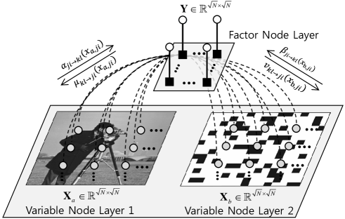
Figure 1: Factor graphical model and message-passing for the $L_{1}$-Split-Analysis problem (5).

II AMP Method for $L_{1}$-Split-Analysis

The first step of the AMP development is to establish a message-passing rule based on a factor graphical model of linear systems. Fig.1 describes a factor graph for our system (1), deriving the corresponding joint PDF, given by

$${f_{{{\mathbf{X}}_{a}},{{\mathbf{X}}_{b}},{\mathbf{Y}}}}(\cdot)\propto{f_{{{\mathbf{X}}_{a}}}}(\cdot;{\mathcal{T}}_{a}){f_{{{\mathbf{X}}_{b}}}}(\cdot;{\mathcal{T}}_{b})\prod\limits_{(k,l)\in\Omega}{{f_{{Y_{kl}}|{{\mathbf{X}}_{a}},{{\mathbf{X}}_{b}}}}(\cdot)}$$ (6)

where the two priors, ${f_{{{\mathbf{X}}_{a}}}}(\cdot;{\mathcal{T}}_{a})$ and ${f_{{{\mathbf{X}}_{b}}}}(\cdot;{\mathcal{T}}_{b})$, sparsify the signals in the domain of ${\mathcal{T}}_{a}$ and ${\mathcal{T}}_{b}$, respectively. From the joint PDF (6), we form a message-passing rule for solving (5) in the manner of the min-sum algorithm [11], given by

$${\text{a) For the signal }}{{\mathbf{X}}_{a}}:\forall(ji,kl)\in\Lambda\times\Omega$$

$$\footnotesize\left\{\begin{gathered}{\mu_{kl\to ji}}({x_{a,ji}})=\mathop{\min}\limits_{\begin{subarray}{l}\{{\mathbf{x}}_{a},\mathbf{x}_{b}\}\\ \backslash{x_{a,ji}}\end{subarray}}\log{f_{{Y_{kl}}|{{\mathbf{X}}_{a}},{{\mathbf{X}}_{b}}}}(\cdot)+\sum\limits_{\begin{subarray}{l}j^{\prime}i^{\prime}\\ \neq ji\end{subarray}}{\alpha_{j^{\prime}i^{\prime}\to kl}}({x_{a,j^{\prime}i^{\prime}}})\hfill\\ \,\,\,\,\,\,\,\,\,\,\,\,\,\,\,\,\,\,\,\,\,\,\,\,\,\,\,\,\,\,\,\,\,\,\,\,\,\,\,\,\,\,\,\,\,\,\,\,\,\,\,\,\,\,\,\,\,\,\,\,\,\,\,\,\,\,\,\,\,\,\,\,\,\,\,\,\,\,\,\,\,\,\,\,\,\,\,\,\,\,\,\,\,\,\,\,\,\,\,\,\,\,\,\,\,\,\,+\sum\limits_{ji\in\Lambda}{{\beta_{ji\to kl}}({x_{b,ji}})}\hfill\\ {\alpha_{ji\to kl}}({x_{a,ji}})=\log{f_{{{\mathbf{X}}_{a}}}}(\mathbf{x}_{a};{\mathcal{T}}_{a})+\sum\limits_{k^{\prime}l^{\prime}\neq kl}{{\mu_{k^{\prime}l^{\prime}\to ji}}({x_{a,ji}})}\hfill\\ \end{gathered}\right.$$ (11)

$${\text{b) For the signal }}{{\mathbf{X}}_{b}}:\forall(ji,kl)\in\Lambda\times\Omega$$

$$\footnotesize\left\{\begin{gathered}{\nu_{kl\to ji}}({x_{b,ji}})=\mathop{\min}\limits_{\begin{subarray}{l}\{{\mathbf{x}}_{a},\mathbf{x}_{b}\}\\ \backslash{x_{b,ji}}\end{subarray}}\log{f_{{Y_{kl}}|{{\mathbf{X}}_{a}},{{\mathbf{X}}_{b}}}}(\cdot)+\sum\limits_{ji\in\Lambda}{{\alpha_{ji\to kl}}({x_{b,ji}})}\hfill\\ \,\,\,\,\,\,\,\,\,\,\,\,\,\,\,\,\,\,\,\,\,\,\,\,\,\,\,\,\,\,\,\,\,\,\,\,\,\,\,\,\,\,\,\,\,\,\,\,\,\,\,\,\,\,\,\,\,\,\,\,\,\,\,\,\,\,\,\,\,\,\,\,\,\,\,\,\,\,\,\,\,\,\,\,\,\,\,\,\,\,\,\,\,\,\,\,\,\,\,\,\,\,\,\,+\sum\limits_{j^{\prime}i^{\prime}\neq ji}{{\beta_{j^{\prime}i^{\prime}\to kl}}({x_{b,j^{\prime}i^{\prime}}})}\hfill\\ {\beta_{ji\to kl}}({x_{b,ji}})=\log{f_{{{\mathbf{X}}_{b}}}}(\mathbf{x}_{b};{\mathcal{T}}_{b})+\sum\limits_{k^{\prime}l^{\prime}\neq kl}{{\nu_{k^{\prime}l^{\prime}\to ji}}({x_{b,ji}})},\hfill\\ \end{gathered}\right.$$ (16)

where $\{\mathbf{x}\}$ indicates the set of elements in the vector argument $\mathbf{x}$. As illustrated in Fig.1, the min-sum rule (II) disjointly exchanges the messages between onefactor layer and two different variable layers where the factor nodes are effective only with the index $(k,l)\in\Omega$, and the variable nodes correspond to the index $(i,j)\in\Lambda$. Then, totally, $4MN$ messages are handled per iteration since there are $M$ effective factors, each of which generates $2N$ messages, and $2N$ variables, each of which produces $M$ messages.

At the fixed-point, the scalar MAP estimate of each signal is approximated by

$$\widehat{x}_{a,ji}=\arg\mathop{\min}\limits_{{x_{a,ji}}\in\mathbb{R}}{\alpha_{ji}}({x_{a,ji}}),\,\,\,\widehat{x}_{b,ji}=\arg\mathop{\min}\limits_{x_{b,ji}\in\mathbb{R}}{\beta_{ji}}({x_{b,ji}}),$$ (17)

where the functions ${\alpha_{ji}}({x_{a,ji}}),{\beta_{ji}}({x_{b,ji}})$, which include the posterior information, are given by

$$\alpha_{ji}({x_{a,ji}})=\log{f_{{{\mathbf{X}}_{a}}}}(\mathbf{x}_{a};{\mathcal{T}}_{a})+\sum\limits_{(k,l)\in\Omega}{{\mu_{kl\to ji}}({x_{a,ji}})},$$ (18)

$$\beta_{ji}({x_{b,ji}})\,=\log{f_{{{\mathbf{X}}_{b}}}}(\mathbf{x}_{b};{\mathcal{T}}_{b})\,+\sum\limits_{(k,l)\in\Omega}{{\nu_{kl\to ji}}({x_{b,ji}})}.$$ (19)

In the AMP literature [9]-[11], the second term of (18),(19) are handled as Gaussian exponents. This is based on the assumption that the factor graph connection, by the matrix $\mathbf{A}$, is sufficiently dense such that the messages ${\mu_{kl\to ji}}({x_{a,ji}}),{\nu_{kl\to ji}}({x_{b,ji}})$ from each factor are Gaussian distributed by the law of large numbers.

Algorithm 1 MixAMP Method

Measurement matrix $\mathbf{A}\in\mathbb{R}^{N\times N}$, Measurements $\mathbf{Y}\in\mathbb{R}^{N\times N}$, Undersampling operator $\mathcal{P}_{\Omega}\{\cdot\}$

Recovered signals $\mathbf{X}_{a}^{t=t^{*}},\mathbf{X}_{b}^{t=t^{*}}\in\mathbb{R}^{N\times N}$

Initialization: ${{\mathbf{R}}^{t=0}}={\mathbf{Y}}$, ${\theta^{t=0}}=\frac{1}{M}\left\|{{{\mathbf{Y}}}}\right\|_{F}^{2}$

$\,\,\,\,\,\,\,\,\,\,\,\,\,\,\,\,\,\,\,\,\,\,\,\,\,\,\,\,\,\,\,\,\,\,\,\,\mathbf{X}_{a}^{t=0}=\mathbf{0},\mathbf{X}_{b}^{t=0}=\mathbf{0}$

for $t=1$ to $t^{*}$ do do

    ${\mathbf{X}}_{a}^{t}=\eta_{a}({{\mathbf{A}}^{T}}{{\mathbf{R}}^{t-1}}{\mathbf{A}}+{\mathbf{X}}_{a}^{t-1};\theta^{t-1})$

    ${\mathbf{X}}_{b}^{t}={\eta_{b}}({{\mathbf{A}}^{T}}{{\mathbf{R}}^{t-1}}{\mathbf{A}}+{\mathbf{X}}_{b}^{t-1};{\theta^{t-1}})$

    $\begin{gathered}{{\mathbf{R}}^{t}}={\mathbf{Y}}-{\mathcal{P}_{\Omega}}\{{\mathbf{A}}({\mathbf{X}}_{a}^{t}+{\mathbf{X}}_{b}^{t}){{\mathbf{A}}^{T}}\}\lx@algorithmicx@hfill\\ \,\,\,\,\,\,\,\,\,\,\,\,\,\,\,\,\,\,\,\,\,\,+{{\mathbf{R}}^{t-1}}\begin{array}[]{l}\frac{N}{M}\end{array}\left\langle{{\eta_{a}}^{\prime}({{\mathbf{A}}^{T}}{{\mathbf{R}}^{t-1}}{\mathbf{A}}+{\mathbf{X}}_{a}^{t-1};{\theta^{t-1}})}\right\rangle\lx@algorithmicx@hfill\\ \,\,\,\,\,\,\,\,\,\,\,\,\,\,\,\,\,\,\,\,\,\,+{{\mathbf{R}}^{t-1}}\begin{array}[]{l}\frac{N}{M}\end{array}\left\langle{{\eta_{b}}^{\prime}({{\mathbf{A}}^{T}}{{\mathbf{R}}^{t-1}}{\mathbf{A}}+{\mathbf{X}}_{b}^{t-1};{\theta^{t-1}})}\right\rangle\lx@algorithmicx@hfill\\ \end{gathered}$

    ${\theta^{t}}=\frac{1}{M}\left\|{{{\mathbf{R}}^{t}}}\right\|_{F}^{2}$

end for

The remaining steps for the AMP development consist of

1. the quadratic approximation step, which approximates the min-sum equations by quadratic functions, then converting (II) to a parameter-passing rule whose messages are simple real numbers (instead of functions),

2. the first-order approximation step, which cancels interference caused by the loopy graph connection, and reduces the number of messages from $4MN$ to $M+2N$.

These development steps are conventional for the AMP methods applied to the other types of linear inverse problems [9]-[11], which are well formulated in the literature [11]. Therefore, we omit details of such remaining steps in this letter, immediately providing a final form of MixAMP in Algorithm 1.

One thing noteworthy is that in Algorithm 1 the two disjoint iterations, described in Fig.1, share the residual term $\mathbf{R}^{t}\in\mathbb{R}^{N\times N}$, which significantly reduces the number of the messages in the iteration. This can be explained using the two arguments given in [11]: i) The messages, sent by the $(k,l)$-th factor, have a residual form through the quadratic approximation step; for example, the message toward the variable index $(a,ji)$ is expressed as

$$r_{a,kl\to ji}=y_{kl}-\mathcal{P}_{\Omega}\left\{\right. \sum\nolimits_{j^{\prime}i^{\prime}\neq ji}a_{i^{\prime}j^{\prime}}a_{j^{\prime}i^{\prime}}x_{a,j^{\prime}i^{\prime}\to kl}$$

$$+\sum\nolimits_{ji\in\Lambda}a_{ij}a_{ji}x_{b,ji\to kl}\left\}\right..$$ (20)

ii) We can drop the directional dependency upon the destination index $(a,ji)$ in (II) by decomposing the residual message $r_{a,kl\to ji}$ into a form of “pure residual + directional correction” under the large limit $M,N\to\infty$, i.e.,

$$r_{a,kl\to ji} =r_{kl}+\delta r_{a,kl\to ji}$$

$$=\underbrace{y_{kl}-\mathcal{P}_{\Omega}\{\sum\nolimits_{ji\in\Lambda}a_{ij}a_{ji}(x_{a,ji\to kl}+x_{b,ji\to kl})\}}_{=r_{kl}}$$

$$\,\,\,\,\,\,\,\,\,\,\,\,\,\,\,\,+\underbrace{a_{ij}a_{ji}x_{a,ji}}_{=\delta r_{a,kl\to ji}},$$ (21)

where the correction term $\delta r_{a,kl\to ji}$ has the order of $\mathcal{O}(N^{-1/2})$. The above two arguments equivalently hold for the factor messages toward the index $(b,ji)$. Therefore, the pure residual $r_{kl}^{t}\in\mathbf{R}^{t}$ is independent of the index of the destination variable, enabling the residual sharing in the two disjoint iteration.

The MixAMP incorporates two distinct denoisers, denoted by $\eta_{a}(\cdot),\eta_{b}(\cdot)$, according to sparsity types in the mixture $\mathbf{X}_{a}+\mathbf{X}_{b}$. These denoisers undertake the sub-optimization tasks given in (17), generating the MAP estimate $\mathbf{X}_{a}^{t},\mathbf{X}_{b}^{t}$ at every iteration. Hence, choice of the sparsifying priors, $f_{\mathbf{X}_{a}}(\cdot),f_{\mathbf{X}_{b}}(\cdot)$, determines functional form of the denoisers; for some choices, we may need to utilize external numerical solvers for the denoiser implementation due to analytical difficulties of the prior exponent e.g., non-scalability and non-smoothness. This denoising concept of MixAMP is analogous to the shrinkage in the context of iterative shrinkage-thresholding (IST). However, they are different in that the MixAMP denoisers shrink $\mathbf{X}_{a}^{t},\mathbf{X}_{b}^{t}$ in the domain of $\mathcal{T}_{a}$ and $\mathcal{T}_{b}$ respectively, whereas the shrinkage operator of IST takes soft-thresholding in the standard domain.

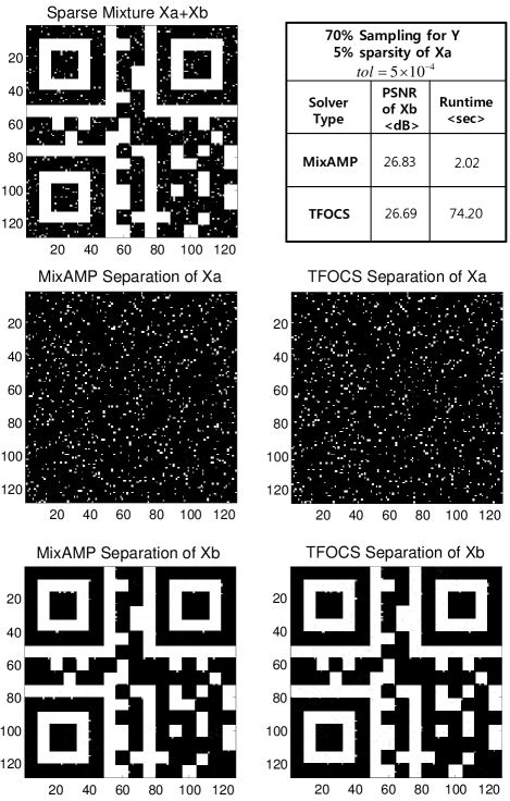
Figure 2: An exemplary comparison of MixAMP and TFOCS in the direct-and-group sparsity separation where we reconstruct a $128\times 128$ QRcode image $\mathbf{X}_{b}$ by removing shot noise $\mathbf{X}_{a}$ (5% sparsity) given the measurements $\mathbf{Y}$ with $70\%$ sampling $(M/N=0.7)$. Here, we set $\varepsilon=10^{-10},\lambda_{1}=0.5,\lambda_{2}=1.2$ for the TFOCS method (27).

III Case Studies for 2D Sparsity Separation

This section provides an exemplary comparison of the MixAMP and the TFOCS [7] methods for two different cases of the sparsity separation. In each case, we first introduce denoisers applied to the MixAMP method, and then we provide the separation example. We inform that the TFOCS method is not directly applicable to the 2D model (1), which should be accompanied by the vectorization of (2). This comparison is based on the standard Gaussian matrix $\mathbf{A}$ whose entries are i.i.d. drawn from $\mathcal{N}(0,\frac{1}{M})$, and MATLAB 2014a with a 2.67-GHz Intel Quad Core i5 was used to generate the results. In addition, we stop the MixAMP and TFOCS iteration when $tol:=\frac{{\sqrt{||{\mathbf{X}}_{a}^{t-1}-{\mathbf{X}}_{a}^{t}||_{F}^{2}+||{\mathbf{X}}_{b}^{t-1}-{\mathbf{X}}_{b}^{t}||_{F}^{2}}}}{{\sqrt{||{\mathbf{X}}_{a}^{t}||_{F}^{2}+||{\mathbf{X}}_{b}^{t}||_{F}^{2}}}}\leq 5\times 10^{-4}$ is met.

III-A Separation of Direct and Group Sparsity

We consider separation of a 2D direct-and-group sparse mixture. For the direct sparsity denoiser, we apply the soft-thresholding which has been the most widely used because of its simplicity [9]. Let $\mathbf{X}_{a}\in\mathbb{R}^{\sqrt{N}\times\sqrt{N}}$ have the direct sparsity. Then, we can estimate $X_{a,ji}\in\mathbb{R}$ via a scalable denoiser $\eta_{a}(\cdot):\mathbb{R}\to\mathbb{R}$, given by

$$\widehat{x}_{a,ji}={\eta_{a}}(x;\theta) :=\arg\mathop{\min}\limits_{{{X}_{a,ji}}}|{X_{a,ji}}|+\frac{\lambda}{2}({X_{a,ji}}-x)^{2}$$

$$=\operatorname{sgn}(x)\max\{|x|-\theta,0\}.$$ (22)

In (III-A), the input $x\in\mathbb{R}$ is a Gaussian variable corresponding to the second term of the posterior function (18). This Gaussianity let the denoiser to solve a penalized least squares problem, which is common in the AMP denoisers. In addition, it is well known that the soft-thresholding is based on the Laplace prior; therefore, we have $\log{f_{{{\mathbf{X}}_{a}}}}({{\mathbf{x}}_{a}})=||\mathbf{X}_{a}||_{1}$ in (18).

We adopt the block soft-thresholding for the group sparsity pursuit [10]. Let $\mathbf{X}_{b}\in\mathbb{R}^{\sqrt{N}\times\sqrt{N}}$ have the group sparsity. Then, the block soft-thresholding denoiser, $\eta_{b}(\cdot):\mathbb{R}^{\sqrt{B}\times\sqrt{B}}\to\mathbb{R}^{\sqrt{B}\times\sqrt{B}}$, is given by

$$\widehat{\mathbf{x}}_{b,B}={\eta_{b}}({{\mathbf{x}}_{B}};\theta) :=\arg\mathop{\min}\limits_{{{\mathbf{X}}_{b,B}}}||{{\mathbf{X}}_{b,B}}||_{F}+\frac{\lambda}{2}||{{\mathbf{X}}_{b,B}}-{{\mathbf{x}}_{B}}||_{F}^{2}$$

$$={{\mathbf{x}}_{B}}\cdot\max\{1-\theta||{{\mathbf{x}}_{B}}||_{F}^{-1},0\}$$ (23)

where the input $\mathbf{x}_{B}\in\mathbb{R}^{\sqrt{B}\times\sqrt{B}}$ is a block matrix such that the signal $\mathbf{X}_{b}$ is partitioned into $N/B$ square blocks with the size $B$. Specifically, this block denoiser makes its block argument $\mathbf{x}_{B}$ to a zero matrix if $||{{\mathbf{x}}_{B}}||_{F}\leq\theta$, otherwise diminishing it by the quantity $\theta$ to the origin. In addition, this block thresholding is related to a block Gaussian prior; hence, we have $\log{f_{{{\mathbf{X}}_{b}}}}({{\mathbf{x}}_{b}})=\sum\nolimits_{{\text{All blocks}}}{||{{\mathbf{X}}_{b,B}}||_{F}}$ from (19).

Fig.2 displays a separation example by MixAMP and TFOCS, where we reconstruct a $128\times 128$ QRcode image $\mathbf{X}_{b}$ by removing shot noise $\mathbf{X}_{a}$ given the measurements $\mathbf{Y}$ with $70\%$ sampling $(M/N=0.7)$. The QR code refers to the group sparsity part of the mixture image, while the shot noise models the direct sparsity part. In the TFOCS method, we recast (5) to Combining-$L_{1}$-and-Group minimization, solving

$$\begin{gathered}\min\,\,\,\lambda_{1}||{{\mathbf{X}}_{a}}|{|_{1}}+\lambda_{2}\sum\limits_{{\text{\tiny All blocks}}}{||{{\mathbf{X}}_{b,B}}|{|_{F}}}\hfill\\ {\text{s.t.}}\,\,\,\,\,||{\mathbf{Y}}-\mathcal{P}_{\Omega}\{{\mathbf{A}}({{\mathbf{X}}_{a}}+{{\mathbf{X}}_{b}}){\mathbf{A}^{T}}\}||_{F}\leq\varepsilon\hfill\\ \end{gathered}$$ (27)

where $\varepsilon,\lambda_{1},\lambda_{2}\geq 0$ are calibration scalars. The result of Fig.2 reports that MixAMP is much faster than TFOCS in CPU runtime while providing comparable reconstruction quality in PSNR.

III-B Separation of Direct and Finite-Difference Sparsity

We present another case by introducing finite-difference (FD) sparsity, then addressing a separation problem with a direct-and-FD sparse mixture. For the FD sparsity pursuit, we apply the total variation (TV) denoiser [10] which has been investigated by the numerous literature (see for example [12]). The TV denoiser is neither scalable nor block-separable because the FD sparsity cannot be defined by a single scalar of the signal, but depending upon all the adjacent of the scalar. Let $\mathbf{X}_{b}\in\mathbb{R}^{\sqrt{N}\times\sqrt{N}}$ have the FD sparsity. Then, we consider the TV denoiser, $\eta_{b}(\cdot):\mathbb{R}^{\sqrt{N}\times\sqrt{N}}\to\mathbb{R}^{\sqrt{N}\times\sqrt{N}}$, which solves

$${\widehat{\mathbf{x}}_{b}}={\eta_{b}}({\mathbf{x}};\lambda):=\arg\mathop{\min}\limits_{{{\mathbf{X}}_{b}}}||\mathbf{X}_{b}||_{\text{TV}}+\frac{\lambda}{2}||{{\mathbf{X}}_{b}}-{\mathbf{x}}||_{F}^{2}.$$ (28)

It is recognizable from (19) that the TV norm $||\mathbf{X}_{b}||_{\text{TV}}$ is the exponent of the sparsifying prior such that $\log{f_{{{\mathbf{X}}_{b}}}}({{\mathbf{x}}_{b}})=||\mathbf{X}_{b}||_{\text{TV}}$. For the implementation of (28), external numerical solvers have been mostly considered since the TV norm is analytically non-scalable and non-smooth [10].

In Fig.3, we simultaneously estimate a shot noise $\mathbf{X}_{a}$ (10% sparsity) and a $128\times 128$ Cameraman image $\mathbf{X}_{b}$ from the 2D measurements $\mathbf{Y}$ with $50\%$ sampling $(M/N=0.5)$. In this example, we postulate that the Cameraman image has the FD sparsity and the shot noise is directly sparse. For the MixAMP separation, we apply the soft-thresholding (III-A) for $\mathbf{X}_{a}$, implementing the anisotropic TV denoising (28) for $\mathbf{X}_{b}$ using the 2D-Bregman iteration (Section 4 of [8]). In the TFOCS method, we recast (5) to Combining-$L_{1}$-and-TV minimization, solving

$$\begin{gathered}\min\,\,\lambda_{1}||{{\mathbf{X}}_{a}}|{|_{1}}+\lambda_{2}||{{\mathbf{X}}_{b}}|{|_{\text{TV}}}\ \hfill\\ {\text{s.t.}}\,\,\,\,||{\mathbf{Y}}-\mathcal{P}_{\Omega}\{{\mathbf{A}}({{\mathbf{X}}_{a}}+{{\mathbf{X}}_{b}}){\mathbf{A}^{T}}\}||_{F}\leq\varepsilon.\hfill\\ \end{gathered}$$ (32)

Likewise to the example in Section III-A, the result of Fig.3 validates the computational advantages of MixAMP where MixAMP is approximately 2 time faster than TFOCS for the same task. The scale difference of the runtime gap from the result of Section III-A is coming from the fact that the Bregman-TV denoiser (28) requires more computations than the block soft-thresholding (III-A) does.

These two comparison results support our claim that MixAMP outperforms the TFOCS method in computational efficiency under the 2D sparse signal separation task.

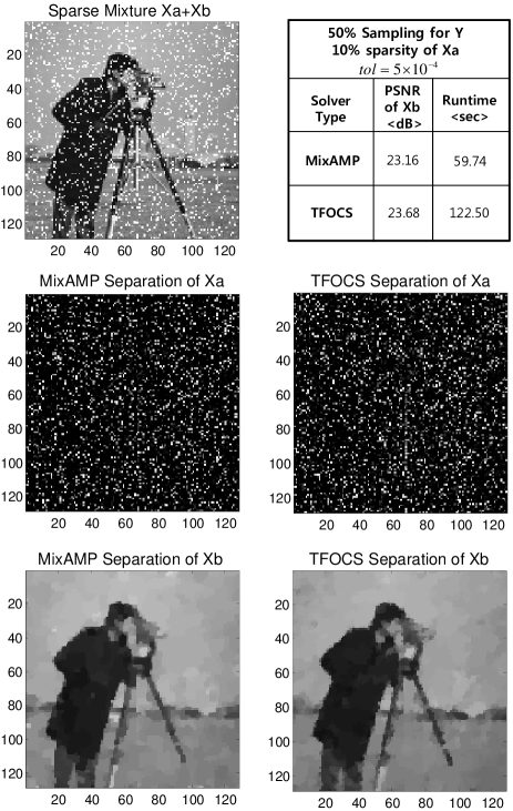
Figure 3: An exemplary comparison of MixAMP and TFOCS in the direct-and-FD sparsity separation where we simultaneously estimate a shot noise $\mathbf{X}_{a}$ (10% sparsity) and a $128\times 128$ Cameraman image $\mathbf{X}_{b}$ from the 2D measurements $\mathbf{Y}$ with $50\%$ sampling $(M/N=0.5)$. Here, we set $\varepsilon=10^{-10},\lambda_{1}=2.0,\lambda_{2}=1.4$ for the TFOCS method (32).

IV Conclusions

In this letter, we have discussed the MixAMP method for the ill-posed $L_{1}$-Split-Analysis, applying the 2D sparse signal separation problem. We first have developed the MixAMP method based on the factor graphical model of the 2D CS measurement model (1). Then, we have provided two cases of the study for the sparsity separation, validating the computational advantages of MixAMP through exemplary comparisons to the conventional first-order method, TFOCS [7]. Therefore, we claim that MixAMP is a very good alternative of the TFOCS method for solving the $L_{1}$-Split-Analysis in the 2D sparse separation problem.

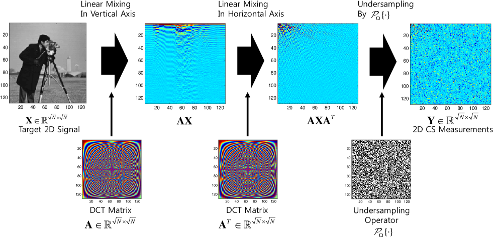
Figure 4: An example of 2D CS measurement generation in the model (1), where we consider the DCT matrix $\mathbf{A}$ and the $128\times 128$ Cameraman image as the 2D target signal $\mathbf{X}$. First, the signal $\mathbf{X}$ is linearly mixed in two perpendicular axes by the DCT matrix $\mathbf{A}$, generating $\mathbf{AXA^{T}}$. Second, the measurement $\mathbf{Y}$ is produced by applying the undersampling operator $\mathcal{P}_{\Omega}\{\cdot\}$ to $\mathbf{AXA^{T}}$.

Supplementary Material

IV-A 2D Compressed Sensing Model (1): A Practical Viewpoint

In this letter, we consider “the compressed sensing (CS) technique” with the model (1). The model (1) requires two-steps for the CS measurement generation of $\mathbf{Y}$ as shown in Fig.4: 1) linear mixing in two perpendicular axes by $\mathbf{AXA^{T}}$ and 2) undersampling by $\mathcal{P}_{\Omega}\{\cdot\}$. One can argue that this two-steps generation makes us to lose an advantage of CS which generates $\mathbf{Y}$ in the first place. Nevertheless, we state that this two-step generation is useful because of two practical reasons:

1. For fast measurement generation with unitary matrices $\mathbf{A}$: The model (1) can provide an accelerated generation of $\mathbf{Y}$ when the matrix $\mathbf{A}$ is some unitary types. For instance, this acceleration utilizes Fast Cosine Transform (FCT) when $\mathbf{A}$ is the DCT matrix, and Fast Fourier Transform when $\mathbf{A}$ is the Fourier matrix. Here, we consider the DCT case as an example. Let $\mathbf{A}_{\text{DCT}}\in\mathbb{R}^{\sqrt{N}\times\sqrt{N}}$ denote the DCT matrix and $\mathbf{A}_{\text{subDCT}}\in\mathbb{R}^{\sqrt{M}\times\sqrt{M}}$ is a sub-DCT matrix whose rows are randomly sampled from $\mathbf{A}_{\text{DCT}}$. The conventional CS generation, expressed as

   $$\mathbf{Y}=\mathbf{A}_{\text{subDCT}}\,\mathbf{X}\,\mathbf{A}_{\text{subDCT}}^{T}\in\mathbb{R}^{\sqrt{M}\times\sqrt{M}},$$ (33)

   spends $\mathcal{O}(NM^{\frac{1}{2}})$ computations due to the matrix multiplications. Compared to (33), the FCT-based generation with the model (1), i.e.,

   $$\mathbf{Y} =\mathcal{P}_{\Omega}\{\mathbf{A}_{\text{DCT}}\,\mathbf{X}\,\mathbf{A}_{\text{DCT}}^{T}\},$$

   $$=\mathcal{P}_{\Omega}\{\text{FCT}_{2D}[\mathbf{X}]\}\in\mathbb{R}^{\sqrt{N}\times\sqrt{N}},$$ (34)

   is computationally efficient with $\mathcal{O}(N\log N^{\frac{1}{2}})$; therefore, its efficiency gets remarkable as the system size $N$ increases. In addition, it is obvious that the FCT method is not applicable with the sub-DCT matrix $\mathbf{A}_{\text{subDCT}}$.

2. Use of a random decimation operator instead of $\mathcal{P}_{\Omega}\{\cdot\}$: In practice, the random undersampling operator $\mathcal{P}_{\Omega}\{\cdot\}$ can be simply replaced by a random decimation operator. Then, the samples of $\mathbf{Y}$ can be stored to a memory with the size $M$ by holding the knowledge of the set $\Omega$. In this case, however, we need an inverse operator of the decimation operator to calculate $\mathbf{A}^{T}\mathbf{R}\mathbf{A}$ for the MixAMP method.

IV-B Hardship of Sparse Separation Problem

The sparsity separation, handled in this letter, is basically harder problem than the conventional single sparsity recovery. This is because the sparsity separation includes not only the reconstruction of the mixture signal $\mathbf{X}$ from the CS measurements $\mathbf{Y}$, but also the separation of the two sparsity, $\mathbf{X}_{a}$ and $\mathbf{X}_{b}$, from the mixture $\mathbf{X}$. We can look at this hardship of the sparsity separation by simple manipulation from (1):

$${\mathbf{Y}}={\mathcal{P}_{\Omega}}\left\{{[{\mathbf{A}}|{\mathbf{A}}]\left[\begin{gathered}{{\mathbf{X}}_{a}}\hfill\\ {{\mathbf{X}}_{b}}\hfill\\ \end{gathered}\right]{{\mathbf{A}}^{T}}}\right\},$$ (38)

From (38), we can reasonably conjecture that the reconstruction of the concatenated signal $[\mathbf{X}_{a}|\mathbf{X}_{b}]^{T}$ from ${\mathbf{Y}}$ requires larger $M$ than the single sparsity recovery does. In addition, while revising this letter, we became aware of a theoretical work of Studer et al. [16] which supports our conjecture by providing a coherence-based sufficient condition for recovery guarantees of ${\mathbf{X}}_{a}$ and ${\mathbf{X}}_{b}$.

Naturally, the reconstruction quality of the sparse separation gets better as the sampling rate $M/N$ increases. In Fig.5, we provide an extended result of the $\mathbf{X}_{b}$ reconstruction in the directed-and-FD sparsity separation (Section III-B) for a variety of $M/N$. From the figure, we see that the both methods improve their reconstruction quality given a higher $M/N$. This result also shows that although the TFOCS method has a small lead in the reconstruction quality as $M/N$ becomes higher, the MixAMP method is still remarkably advantageous in computational cost.

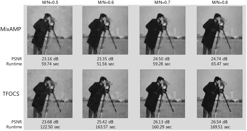
Figure 5: Extended numerical result of the directed-and-FD sparsity separation in Section III-B: In this figure, we only plot reconstruction of the $128\times 128$ Cameraman image $\mathbf{X}_{b}$ for a variety of the sampling rate $M/N$. The others for the experimental setup remains the same as Section III-B. For the TFOCS method (15), we use empirically-tuned parameter set $(\lambda_{1},\lambda_{2},\varepsilon)$.

References

• [1] N. Zhou, H. Li, D. Wang, S. Pan, and Z. Zhou, “Image compression and encryption scheme based on 2D compressive sensing and fractional Mellin transform,” Optics Communi., vol. 343, pp. 10-21, May. 2015.
• [2] M. F. Duarte, and R. G. Baraniuk, “Kronecker compressive sensing,” IEEE Trans. Image. Process. vol. 21, no. 2, pp. 494-504, Feb. 2012
• [3] E. J. Candes, Y. C. Eldar, D. Needell, and P. Randall, “Compressed sensing with coherent and redundant dictionaries,” Appl. Comput. Harmon. Anal., vol. 31, no. 1, pp. 59-73, Sep. 2011.
• [4] C. Aubel, C. Studer, G. Pope, H. Bolcskei, “Sparse signal separation in redundant dictionaries,” in Proc. IEEE Intl. Symp. on Inf. Theory, ISIT, Boston, MA, USA, pp. 2047-2051, 2012.
• [5] J.-F. Cai, S. Osher, and Z. Shen, “Split Bregman methods and frame based image restoration,” Multiscale Modeling and Simulation, vol. 8, no. 2, pp. 337-369, Jan. 2010.
• [6] S. G. Mallat and G. Yu, “Super-resolution with sparse mixing estimators,” IEEE Trans. Image Process., vol. 19, no. 11, pp. 2889-2900, Nov. 2010.
• [7] S. Becker, E. J. Candes and M. Gran, “Templates for Convex Cone Problems with Applications to Sparse Signal Recovery,” Math. Program. Comput., vol. 3, num. 3, Aug. 2011. MATLAB code available at http://cvxr.com
• [8] T. Goldstein and S. Osher. “The split Bregman algorithm for l1 regularized problems,” SIAM J. Imaging Sciences, vol. 2, pp. 323-343, Apr. 2009.
• [9] D.L. Donoho, A. Maleki, and A. Montanari, “Message passing algorithms for compressed sensing,” Proc. Nat. Acad. Sci., vol. 106, pp. 18914-18919, Nov. 2009.
• [10] D.L. Donoho, I. Johnstone, and A. Montanari, “Accurate prediction of phase transitions in compressed sensing via a connection to minimax denoising, ” IEEE Trans. Inform. Theory, vol. 59, no. 6, pp. 3396-3433, June 2013.
• [11] A. Montanari, “Graphical models concepts in compressed sensing,” available at arXiv:1011.4328v3[cs.IT], Mar. 2011.
• [12] L.I. Rudin, S. Osher, and E. Fatemi, “Nonlinear total variation based noise removal algorithms,” Physica D:Nonlinear Phenomena, vol. 60, pp. 259-268, Nov. 1992.
• [13] J. Starck, M. Elad, and D. Donoho,“Image decomposition via the combination of sparse representations and a variational approach,”
• [14] J. Bobin, J. L. Starck, J. M. Fadili, Y. Moudden, and D. L. Donoho, “Morphological component analysis: An adaptive thresholding strategy,” IEEE Trans. Image Process., vol. 16, no. 11, pp. 2675-2681, Nov. 2007.
• [15] J. Ma, G. Plonka, M. Y. Hussaini, “Compressive video sampling with approximate message passing decoding,” IEEE Trans. Circuits Syst. Video Technol., vol. 22, no. 9, pp. 1354-1364, Sep. 2012.
• [16] C. Studer, P. Kuppinger, G. Pope, and H. Bolcskei, “Recovery of sparsely corrupted signals,” IEEE Trans. Inform. Theory, vol. 58, no. 5, pp. 3115-3130, May 2012.