Summary. While death rates due to diseases of the heart have experienced a sharp decline over the past 50 years, these diseases continue to be the leading cause of death in the United States, and the rate of decline varies by geographic location, race, and gender. We look to harness the power of hierarchical Bayesian methods to obtain a clearer picture of the declines from county-level, temporally varying heart disease death rates for men and women of different races in the US. Specifically, we propose a nonseparable multivariate spatio-temporal Bayesian model which allows for group-specific temporal correlations and temporally-evolving covariance structures in the multivariate spatio-temporal component of the model. After verifying the effectiveness of our model via simulation, we apply our model to a dataset of over 200,000 county-level heart disease death rates. In addition to yielding a superior fit than other common approaches for handling such data, the richness of our model provides insight into racial, gender, and geographic disparities underlying heart disease death rates in the US which are not permitted by more restrictive models.

Key words: Bayesian methods, Gender disparities in health, Heart disease, Nonseparable models, Racial disparities in health, Spatio-temporal data analysis

1 Introduction

Despite substantial reductions in death rates since the mid-1960s (e.g., Sempos et al.,, 1988; Ford and Capewell,, 2011; Young et al.,, 2010; Greenlund et al.,, 2007), heart disease remains the leading cause of death in the United States (US, Murphy et al.,, 2013). Work by Casper et al., (2015) has identified that while the nation as a whole has experienced substantial declines in heart disease mortality rates, there has been a substantial geographic shift over time, as mortality rates in the northeast have declined at a much faster rate than those in the Deep South. Previous work has also shown disparities in heart disease death rates between the sexes (e.g., Sempos et al.,, 1988; Kramer et al.,, 2015), between races (e.g., Kramer et al.,, 2015), and geographically (e.g., Gillum et al.,, 2012; Vaughan et al.,, 2014, 2015), yet accounting for these various sources of disparities simultaneously has yet to be considered. Here, we look to build upon the existing heart disease literature to obtain a broader picture of these declining death rates using a hierarchical Bayesian statistical approach which accounts for correlation spatially, temporally, and between race/gender groups.

There is an extensive literature on the subject of space-time modeling, particularly in the Bayesian context. A common approach for modeling discrete — or areal — spatial data is the use of the conditionally autoregressive (CAR) model proposed by Besag, (1974) and later popularized in the disease mapping context by Besag et al., (1991). Early uses of the CAR model in the space-time setting include Waller et al., (1997) and Knorr-Held and Besag, (1998) — both of which analyzed rates of lung cancer in Ohio counties — and Gelfand et al., (1998), whose interest pertained to the sale prices of homes. While these methods have used separable model structures for space and time, Knorr-Held, (2000) discusses the use of nonseparable space-time models in a discrete space, discrete time setting with an application to lung cancer mortality rates in Ohio. In addition to space-time data models, Gelfand and Vounatsou, (2003) and Carlin and Banerjee, (2003) have developed methods for general multivariate spatial models. For a more complete coverage of the recent advances in spatial and space-time modeling, see Cressie and Wikle, (2011) and Banerjee et al., (2014).

The concept of multivariate space-time (MST) models for discrete spatial data has also been explored previously. For instance, Congdon, (2002) modeled suicide mortality rates in the boroughs of London using spatially varying regression coefficients and a nonparametric specification of the random effects, and Daniels et al., (2006) developed a conditionally specified model for the analysis of particulate matter and ozone data collected from monitoring sites in Los Angeles, CA. More recently, Bradley et al., (2014) proposed an alternative in which the authors use a shared component model (e.g., Knorr-Held and Best,, 2001; Tzala and Best,, 2008) with a reduced-rank spatial domain, extending the approach of Hughes and Haran, (2013) to the MST setting. While a shared component model can offer substantial computational benefits by effectively reducing the complexity of a MST model to that of a reduced-rank space-time model, this assumption may not always be appropriate (e.g., when the available covariate information is insufficient to capture the differences in the geographic patterns) nor necessary (e.g., when number of groups in the multivariate structure is small).

Due to the recent geographic and temporal evolutions in heart disease death rates, the methodological goal of this paper is to define a nonseparable multivariate space-time modeling framework to analyze the heart disease mortality rate data described in Section 2. We propose our model in Section 3 and demonstrate its ability to accurately estimate model parameters via simulation study in Section 4. We then analyze our heart disease mortality data in Section 5, where we observe temporally-evolving variance parameters inconsistent with the previously used separable model. Finally, we summarize our findings and offer some concluding remarks in Section 6.

2 Data Description

The study population for this analysis includes US residents, ages 35 and older, who were identified on a death certificate as either black or white — we restrict our analysis to these $N_{g}=4$ groups because these are the only racial groups for whom data are available for the entire duration of our study period. Annual counts of heart disease deaths per county per race/gender group were obtained from the National Vital Statistics System (NVSS) of the National Center for Health Statistics (NCHS). Due to differences in the manner in which death records were processed by NCHS, we restrict the analysis to data from 1973–2010 to ensure valid comparisons across time. Deaths from heart disease were defined as those for which the underlying cause of death was “diseases of the heart” according to the 8th, 9th, and 10th revisions of the International Classification of Diseases (ICD). Based on the works of Klebba and Scott, (1980) and Anderson et al., (2001), we assume that this definition is consistent over the 38 year study period. Annual projected population counts were obtained from the NCHS, (2013), and the numbers of heart disease deaths were age-standardized to the 2000 US Standard Population using 10 year age groups.

The geographic unit used in this analysis was the county (or county equivalent). Given changes in county definitions during the study period (e.g., the creation of new counties), a single set of $N_{s}$ = 3,099 counties from the contiguous lower 48 states was used for the entire study period. In an attempt to stabilize the data, county-level age-standardized counts and populations were aggregated into $N_{t}=19$ two year intervals (i.e., 1973–74, 1975–76, etc.).

3 Methods

3.1 Review of methods for disease mapping

One of the seminal papers in the field of disease mapping was the work of Besag et al., (1991). Letting $Y_{i}$ and $n_{i}$ denote the incidence of disease and the population at risk in county $i$, the authors proposed a model of the form

$$Y_{i}\sim\mbox{$\text{Pois}$}\left(n_{i}\exp\left[{\bf x}_{i}\boldsymbol{\beta}+Z_{i}+\phi_{i}\right]\right),i=1,\ldots,N_{s}$$ (1)

where ${\bf x}_{i}$ denotes a $p$-vector of covariates with corresponding regression coefficients, $\boldsymbol{\beta}$, $Z_{i}$ is a spatial random effect, and $\phi_{i}\sim N\left(0,\tau^{2}\right)$ is an exchangeable random effect. In their work, Besag et al., (1991) modeled ${\bf Z}=\left(Z_{1},\ldots,Z_{N_{s}}\right)^{\prime}$ as arising from an intrinsic conditional autoregressive (CAR) model, which has the conditional distribution

$$Z_{i}\,|\,{\bf Z}_{(i)},\sigma^{2}\sim N\left(\sum_{j=1}^{N_{s}}w_{ij}Z_{j}/\sum_{j=1}^{N_{s}}w_{ij},\sigma^{2}/\sum_{j=1}^{N_{s}}w_{ij}\right)$$ (2)

where ${\bf Z}_{(i)}$ denotes the vector ${\bf Z}$ with the $i$th element removed and $W$ is an adjacency matrix with elements $w_{ij}=1$ if $i$ and $j$ are neighbors (denoted $i\sim j$) and 0 otherwise. Later work by Knorr-Held, (2002) and Hodges et al., (2003) has shown that the joint distribution of ${\bf Z}$ in (2) is of the form

$$\pi\left({\bf Z}\,|\,\sigma^{2}\right)\propto\left(\sigma^{2}\right)^{-(N_{s}-1)/2}\exp\left[-\frac{1}{2\sigma^{2}}{\bf Z}^{\prime}(D-W){\bf Z}\right],$$ (3)

where $D$ is an $N_{s}\times N_{s}$ diagonal matrix with elements $m_{i}=\sum_{j=1}^{N_{s}}w_{ij}$.

Extending (1)–(3) to a setting consisting of multiple spatial surfaces is straightforward. For instance, suppose we wish to map $N_{g}$ diseases over an area consisting of $N_{s}$ counties. Letting $Y_{ik}$ denote the incidence of disease $k$ in county $i$, we may assume

$$Y_{ik}\sim\mbox{$\text{Pois}$}\left(n_{ik}\exp\left[{\bf x}_{ik}\boldsymbol{\beta}_{k}+Z_{ik}+\phi_{ik}\right]\right),i=1,\ldots,N_{s},\;k=1,\ldots,N_{g}.$$ (4)

To model ${\bf Z}=\left({\bf Z}_{1\cdot}^{\prime},\ldots,{\bf Z}_{N_{s}\cdot}^{\prime}\right)^{\prime}$ where ${\bf Z}_{i\cdot}=\left(Z_{i1},\ldots,Z_{iN_{g}}\right)^{\prime}$, we may follow the example of Gelfand and Vounatsou, (2003) and let ${\bf Z}\sim\mbox{$\text{MCAR}$}\left(1,\mbox{$\Sigma$}_{Z}\right)$ which yields the following:

$$\pi\left({\bf Z}\,|\,\mbox{$\Sigma$}_{Z}\right) \propto|\mbox{$\Sigma$}_{Z}|^{(N_{s}-1)/2}\exp\left[-\frac{1}{2}{\bf Z}^{\prime}\left\{(D-W)\otimes\mbox{$\Sigma$}_{Z}^{-1}\right\}{\bf Z}\right]$$

$$\text{and}\;\;{\bf Z}_{i\cdot}\,|\,{\bf Z}_{(i)\cdot},\mbox{$\Sigma$}_{Z} \sim N\left(\sum_{j\sim i}{\bf Z}_{j\cdot}/m_{i},\frac{1}{m_{i}}\mbox{$\Sigma$}_{Z}\right),$$

where $\mbox{$\Sigma$}_{Z}$ denotes the $N_{g}\times N_{g}$ covariance structure for our $N_{g}$ diseases and $\otimes$ denotes the Kronecker product. Extensions of (1) to the (multivariate) space-time setting follow similarly (e.g., Zhu et al.,, 2013), with the necessary specifications of the covariance matrix $\mbox{$\Sigma$}_{Z}$.

While Poisson models like (4) are common, they can also pose computational challenges. For instance, the full conditional of ${\bf Z}_{i}$, given by

$$\pi\left({\bf Z}_{i}\,|\,{\bf Y},{\bf Z}_{(i)\cdot},\boldsymbol{\beta},\mbox{\boldmath$\phi$},\mbox{$\Sigma$}_{Z}\right)\propto\prod_{k=1}^{N_{g}}\mbox{$\text{Pois}$}\left(Y_{ik}\,|\,\boldsymbol{\beta}_{k},Z_{ik},\phi_{ik}\right)\times\pi\left({\bf Z}_{i}\,|\,{\bf Z}_{(i)\cdot},\mbox{$\Sigma$}_{Z}\right)$$ (5)

is not a known distribution. That is, if we use a Markov chain Monte Carlo (MCMC) algorithm to estimate the posterior distribution of our model parameters, this model may require the use of Metropolis steps within our Gibbs sampler. When the number of groups is large — or in the space-time setting when $N_{t}$ is large — updating ${\bf Z}$ can be cumbersome. Besag et al., (1995) suggests a reparameterization of (4) which would involve integrating $\phi_{ik}$ out of the model, yielding a Gaussian full conditional for ${\bf Z}_{i}$, though this model still consists of over twice as many parameters as data points.

One alternative to modeling the counts using a Poisson likelihood is to model the rates as being log-normally distributed. For instance, suppose $Y_{ikt}$ and $n_{ikt}$ denote the number of heart disease-related deaths and the population at risk for the $k$th population in county $i$ at time $t$, respectively. We could then model $\theta_{ikt}=\log\left(Y_{ikt}/n_{ikt}\right)$ using a Gaussian distribution. This may be problematic, however, as our data consist of a large number of counties experiencing zero deaths related to heart disease for a given population in a given year. As such, this may require us to treat $Y_{ikt}=0$ as data below the limit of detection by substituting $Y_{ikt}=Y_{ikt}^{*}<1$ or by multiply imputing values for $Y_{ikt}$ (e.g., see Fridley and Dixon,, 2007).

In order to avoid the computational burden associated with the Poisson model in (1) and the ill-handling of zeros in the log-normal model, we opt to model the rates themselves as Gaussian. That is, we let $Y_{ikt}$ denote the age-standardized death rate (per 100,000) in county $i\in\{1,\ldots,N_{s}\}$ during time interval $t=\{1,\ldots,N_{t}\}$ for race/gender group $k\in\{1,\ldots,N_{g}\}$ and we define ${\bf Y}_{i\cdot t}$ to be the vector collecting the $N_{g}$ observations from time $t$ in the $i$th county, ${\bf Y}_{i\cdot\cdot}=\left({\bf Y}_{i\cdot 1}^{\prime},\ldots,{\bf Y}_{i\cdot N_{t}}^{\prime}\right)^{\prime}$ to be the vector collecting the $\left(N_{g}N_{t}\right)$ observations from the $i$th county, and ${\bf Y}=({\bf Y}_{1\cdot\cdot}^{\prime},\ldots,{\bf Y}_{N_{s}\cdot\cdot}^{\prime})^{\prime}$ to be the $N_{s}N_{g}N_{t}$-vector which stacks all of the age-standardized death rates. To model the death rates, we assume

$$Y_{ikt}\sim N\left({\bf x}_{ikt}^{\prime}\boldsymbol{\beta}_{k}+Z_{ikt},\tau_{ikt}^{2}\right),\;i=1,\ldots,N_{s},\;k=1,\ldots,N_{g},\;t=1,\ldots,N_{t}$$ (6)

where ${\bf x}_{ikt}$ is the $p\times 1$ vector of covariates for the $i$th county at time $t$ with a corresponding $p\times 1$ vector of regression coefficients, $\boldsymbol{\beta}_{k}$, $Z_{ikt}$ is a random effect which accounts for the spatio-temporal dependence between and within the four race/gender groups, $\tau_{ikt}^{2}=\tau_{k}^{2}/n_{ikt}$, and $n_{ikt}$ denotes the population of group $k$ in county $i$ at time $t$ divided by 100,000. A recent example of a model of this form is Quick et al., (2013), where a Gaussian likelihood was used to model changes in county-level asthma hospitalization rates in California. We provide a defense of the Gaussian assumption for these data in Figure B.1 of the Web Appendix.

3.2 Choices for $\mbox{$\Sigma$}_{Z}$

Before we present our proposed MSTCAR model for $\mbox{$\Sigma$}_{Z}$ in Section 3.2.3, we begin by describing other natural choices: independence models and a separable model. Not only do these models have computational benefits, but they are also special cases of the MSTCAR.

3.2.1 Independence models

Based on the multivariate spatial models described in Section 3.1, one could opt to fit a collection of $N_{g}$ independent space-time models (denoted STCAR) of the form

$${\bf Z}_{ik\cdot}\,|\,{\bf Z}_{(i)k\cdot},\sigma_{k}^{2},\rho_{k} \sim N\left(\frac{1}{m_{i}}\sum_{j\sim i}{\bf Z}_{jk\cdot},\frac{\sigma_{k}^{2}}{m_{i}}R\left(\rho_{k}\right)\right),k=1,\ldots,N_{g}$$ (7)

where $R\left(\rho_{k}\right)$ denotes an $N_{t}\times N_{t}$ temporal correlation matrix with parameter $\rho_{k}$ and $\sigma_{k}^{2}$ is the variance parameter corresponding to race/gender group $k$. In addition to accounting for spatiotemporal correlation, a model of the form (6) with this structure for ${\bf Z}$ has the added computational benefit of being able to be fit in parallel as $N_{g}$ separate models. This convenience, however, comes at the cost of failing to account for the correlation between groups. As we believe there to be a high degree of correlation between the heart disease mortality rates of our various race/gender groups, this drawback is particularly disappointing.

We could also choose to fit $N_{t}$ independent multivariate spatial models of the form

$${\bf Z}_{i\cdot t}\,|\,{\bf Z}_{(i)\cdot t},G_{t} \sim N\left(\frac{1}{m_{i}}\sum_{j\sim i}{\bf Z}_{j\cdot t},\frac{1}{m_{i}}G_{t}\right),$$

where $G_{t}$ denotes a temporally-varying $N_{g}\times N_{g}$ multivariate covariance structure for our race/gender groups. While this model can also have substantial computational benefits, the assumption of temporal independence is especially damning.

3.2.2 Separable model

Driven by the desire to account for both temporal and between-group correlation in our spatial model, a separable model of the form

$${\bf Z}_{i\cdot\cdot}\,|\,{\bf Z}_{(i)\cdot\cdot},G,\rho \sim N\left(\frac{1}{m_{i}}\sum_{j\sim i}{\bf Z}_{j\cdot\cdot},\frac{1}{m_{i}}R(\rho)\otimes G\right),$$ (8)

where we let $R\left(\rho\right)$ denote an $N_{t}\times N_{t}$ temporal correlation matrix and $G$ denote the $N_{g}\times N_{g}$ between-group covariance structure, may be attractive. The appeal of a separable model where $\mbox{$\Sigma$}_{Z}=R(\rho)\otimes G$ is immediately clear: instead of accounting for multivariate temporal correlation using an unstructured $N_{g}N_{t}\times N_{g}N_{t}$ matrix, $\mbox{$\Sigma$}_{Z}$, we can separate our problem into matrices of rank $N_{g}$ and $N_{t}$, reducing the computational complexity of inverting $\mbox{$\Sigma$}_{Z}$ substantially. While the criticism of separable models in the spatiotemporal literature is primarily directed toward their use in the continuous space, continuous time setting where prediction at unobserved locations is of interest (e.g., see Stein,, 2005), the lack of a temporally evolving $G_{t}$ or group-specific $\rho_{k}$ may be undesirable.

3.2.3 The MSTCAR model

To construct our random effects, ${\bf Z}$, we will begin by defining ${\bf v}_{\iota\cdot t}\mbox{$\stackrel{{\scriptstyle\text{iid}}}{{\sim}}$}N(\textbf{0},G_{t})$ to be a collection of independent $N_{g}$-dimensional random variables with covariance $G_{t}$ for $\iota=1,\ldots,(N_{s}-1)$ and $t=1,\ldots,N_{t}$. Note the deliberate use of the subscript $\iota$ instead of the subscript $i$; this is to reinforce that ${\bf v}_{\iota\cdot t}$ does not correspond to a particular county. From this, we define ${\bf v}_{\iota k\cdot}=\left(v_{\iota k1},\ldots,v_{\iota kN_{t}}\right)^{\prime}$ and construct

$$\mbox{\boldmath$\eta$}_{\iota k\cdot}=\widetilde{R}_{k}{\bf v}_{\iota k\cdot}\sim N\left(\textbf{0},\widetilde{R}_{k}G_{k,k}^{*}\widetilde{R}_{k}^{\prime}\right),\;\iota=1,\ldots,(N_{s}-1),\;k=1,\ldots,N_{g},$$ (9)

where we define $\widetilde{R}_{k}$ to be the Cholesky decomposition of $R_{k}$ such that $\widetilde{R}_{k}\widetilde{R}_{k}^{\prime}=R_{k}$, where $R_{k}\equiv R\left(\rho_{k}\right)$ is a temporal correlation matrix based on an autoregressive order 1 — or AR(1) — structure with correlation parameter $\rho_{k}$ and $G_{k,k}^{*}$ is the $N_{t}\times N_{t}$ diagonal matrix with elements $\left\{G_{t}\right\}_{k,k}$ for $t=1,\ldots,N_{t}$. Equivalently, we can define $\mbox{\boldmath$\eta$}_{\iota\cdot\cdot}\sim N\left(\textbf{0},\mbox{$\Sigma$}_{\eta}\right)$ where

$$\mbox{$\Sigma$}_{\eta}=\begin{bmatrix}\widetilde{R}_{1,1}^{*}&\textbf{0}&\textbf{0}\\ \vdots&\ddots&\textbf{0}\\ \widetilde{R}_{N_{t},1}^{*}&\cdots&\widetilde{R}_{N_{t},N_{t}}^{*}\end{bmatrix}\begin{bmatrix}G_{1}&\textbf{0}&\textbf{0}\\ \textbf{0}&\ddots&\textbf{0}\\ \textbf{0}&\textbf{0}&G_{N_{t}}\end{bmatrix}\begin{bmatrix}\widetilde{R}_{1,1}^{*}&\cdots&\widetilde{R}_{N_{t},1}^{*}\\ \textbf{0}&\ddots&\vdots\\ \textbf{0}&\textbf{0}&\widetilde{R}_{N_{t},N_{t}}^{*}\end{bmatrix},$$ (10)

where $\widetilde{R}_{t,t^{\prime}}^{*}$ denotes the $N_{g}\times N_{g}$ diagonal matrix with elements $\left\{\widetilde{R}_{k}\right\}_{t,t^{\prime}}$ for $k=1,\ldots,N_{g}$. Finally, we let $\mbox{$\Sigma$}_{Z}\equiv\mbox{$\Sigma$}_{\eta}$ and define ${\bf Z}$ in the form of an $\mbox{$\text{MCAR}$}\left(1,\mbox{$\Sigma$}_{\eta}\right)$ of Gelfand and Vounatsou, (2003) with a conditional and (improper) joint distribution of

$${\bf Z}_{i\cdot\cdot}\,|\,{\bf Z}_{(i)\cdot\cdot},G_{1},\ldots,G_{N_{t}},\mbox{\boldmath$\rho$}\sim \;N\left(\frac{1}{m_{i}}\sum_{j\sim i}{\bf Z}_{j},\frac{1}{m_{i}}\mbox{$\Sigma$}_{\eta}\right),\;i=1,\ldots,N_{s}$$ (11)

$$\pi\left({\bf Z}\,|\,G_{1},\ldots,G_{N_{t}},\mbox{\boldmath$\rho$}\right)\propto \;|\mbox{$\Sigma$}_{\eta}|^{-(N_{s}-1)/2}\exp\left[-\frac{1}{2}{\bf Z}^{\prime}\left\{(D-W)\otimes\mbox{$\Sigma$}_{\eta}^{-1}\right\}{\bf Z}\right],$$ (12)

respectively. We denote the expression in (12) as ${\bf Z}\sim\mbox{$\text{MSTCAR}$}\left(G_{1},\ldots,G_{N_{t}},\mbox{\boldmath$\rho$}\right)$.

3.3 Hierarchical model

We complete the hierarchial model by specifying prior distributions for the remaining parameters. As is common in Bayesian modeling, we place a flat, noninformative prior on $\boldsymbol{\beta}_{k}$, and, following Gelman, (2006), assume an improper uniform prior over the positive real numbers for $\tau_{k}$. For each of the spatio-temporal covariance matrices, $G_{t}$, we assume an inverse Wishart distribution with positive definite scale matrix $G$ and $\nu>N_{g}-1$ degrees of freedom, and we use Beta priors for each of the $\rho_{k}$s. Finally, as many rural counties (particularly in the north-central states) have no data from the black populations, we decompose ${\bf Y}$ as ${\bf Y}_{c}=\left({\bf Y}_{o}^{\prime},{\bf Y}_{u}^{\prime}\right)^{\prime}$, where ${\bf Y}_{o}$ denotes the vector of counties with observed populations and ${\bf Y}_{u}$ denotes the vector of counties with unobserved populations. Putting these pieces together, the full hierarchical model is as follows:

$$\pi\left(\boldsymbol{\beta},{\bf Z},G_{1},\ldots,G_{t},\mbox{\boldmath$\rho$},\mbox{\boldmath$\tau$}^{2},{\bf Y}_{u}\,|\,{\bf Y}_{o}\right)\propto N\left({\bf Y}\,|\,X\boldsymbol{\beta}+{\bf Z},\mbox{$\Sigma$}_{Y}\right)\times\mbox{$\text{MSTCAR}$}\left({\bf Z}\,|\,G_{1},\ldots,G_{N_{t}},\mbox{\boldmath$\rho$}\right)$$

$$\times\prod_{k=1}^{N_{g}}\left[\mbox{$\text{Beta}$}\left(a_{\rho},b_{\rho}\right)\times\pi\left(\tau_{k}^{2}\right)\right]$$

$$\times\prod_{t=1}^{N_{t}}\mbox{$\text{InvWish}$}\left(G_{t}\,|\,G,\nu\right),$$ (13)

where the notation $\pi(x)$ denotes the marginal distribution for a random variable $x$ and $\pi(x\,|\,y)$ denotes the conditional distribution of $x$ given $y$. Here, $\mbox{$\Sigma$}_{Y}$ is a diagonal matrix with elements $\tau_{ikt}^{2}$, $X$ is the $(N_{s}N_{g}N_{t}\times p)$ matrix of covariates, and $\pi\left(\tau_{k}^{2}\right)$ is the density for $\tau_{k}^{2}$ which corresponds to a flat prior for $\tau_{k}$. In cases where it may be difficult to learn about each $G_{t}$ or each $\rho_{k}$, we may consider putting additional structure on the priors for these parameters. Note that in (3.3), ${\bf Y}_{u}$ is treated as an unknown model parameter, and thus each $Y_{ikt}\in{\bf Y}_{u}$ is sampled from (6) during each iteration of the MCMC algorithm. Furthermore, we assign a small value for each $n_{ikt}$ in the set $\{n_{ikt}:Y_{ikt}\in{\bf Y}_{u}\}$. A detailed derivation of the MCMC sampler used for this analysis, as well as a description of the benefits of using an AR(1) model to account for temporal correlation, can be found in Web Appendix A.

4 Simulation Study

To evaluate the ability of our model to accurately estimate all of our model parameters, we devised two simulation studies, each comprised of $L=100$ sets of data generated using our MSTCAR model with $N_{t}=10$ timepoints, $N_{g}=3$ groups, and the $N_{s}=58$ counties of California as our spatial domain. This spatial domain offered a compromise between creating a computationally feasible simulation study (compared to using all 3,099 county equivalents) while representing a state with a moderate number of counties and variation in population density and geographic spread. The first simulation study assumes that $n_{ikt}\equiv n$ for all combinations of $(i,k,t)$, allowing us to focus on parameter estimation irrespective of the amount of information each county can provide. We will then relax this assumption by generating data using actual populations of California counties.

In each simulation study, performance was primarily assessed via coverage (i.e., the percent of 95% credible intervals (95% CI) which cover the true parameter values) where values near 95% are desired. Furthermore, we will compare results from the MSTCAR model proposed here to those obtained using a separable model. While the separable model will be incapable of providing accurate estimates for the many additional parameters which comprise $\mbox{$\Sigma$}_{\eta}$, the focus here will be on model fit. Specifically, we will compare the coverage of ${\bf Z}$ and the deviance information criterion (DIC) of Spiegelhalter et al., (2002), where lower values indicate a better compromise of model fit and model complexity.

4.1 Equal population sizes

The $\ell$th dataset is created by generating $Y_{ijk}^{(\ell)}\sim N(Z_{ijk}^{(\ell)},\tau_{k}^{2})$ where $\tau_{k}^{2}=1$ for $k=1,\ldots,N_{g}$ and ${\bf Z}^{(\ell)}$ is drawn from the MSTCAR model in (12). To do this, we first let $\mbox{\boldmath$\rho$}=(0.8,0.85,0.90)^{\prime}$ and generated samples of $G_{t}$ from an inverse Wishart distribution with $2*N_{g}+1$ degrees of freedom and scale matrix $20*N_{g}*I_{N_{g}}$, where $I_{N_{g}}$ is the identity matrix of size $N_{g}$. Using these parameters to construct $\mbox{$\Sigma$}_{\eta}$ (from which all $L$ datasets are based), we generated our latent variables $\mbox{\boldmath$\eta$}_{\iota\cdot\cdot}^{(\ell)}\sim N\left(\textbf{0},\mbox{$\Sigma$}_{\eta}\right)$. From these, we used the methods described in Rue and Held, (2005) to generate our ${\bf Z}^{(\ell)}$; specifically, we found the eigenvalues and eigenvectors of the matrix $D-W$ (based on the adjacencies of counties in California) and used the linear dependence of the eigenvectors to generate our spatial structure. Each simulated dataset is then analyzed using the hierarchical model in (3.3) using MCMC. Using the priors described in the previous section, we initialized all of our parameters (including ${\bf Z}$) at their true values, resulting in chains which were quick to converge and allowing us to assess the performance of our model using just 1,500 iterations of our MCMC algorithm, the last 500 of which were used as the basis for our results. In order to better visualize these results, we also display results from an arbitrarily selected dataset.

Overall, our model performed quite well. Collectively, the $Z_{ikt}$ were well estimated, as demonstrated in Figure 1, with our model obtaining 94.4% coverage and offering an improvement in DIC in 82 of the 100 datasets. This accuracy is permitted due in part to the flexibility of our model to allow for temporally evolving $G_{t}$. As shown in Figure 2, the randomly generated $G_{t}$ exhibited some irregular behavior. While the MSTCAR model was able to estimate these $G_{t}$ quite well — with 95.4% coverage for the diagonal elements (i.e., the variances) and 95.3% coverage for the off-diagonal elements (i.e., the covariances) — the separable model fails to accommodate such a nuanced multivariate structure. We also achieved accurate estimates of the error variances, $\tau_{k}^{2}$, for which we obtained an average of 91.3% coverage. In contrast, coverage for $\rho_{k}$ was less than ideal (85%).

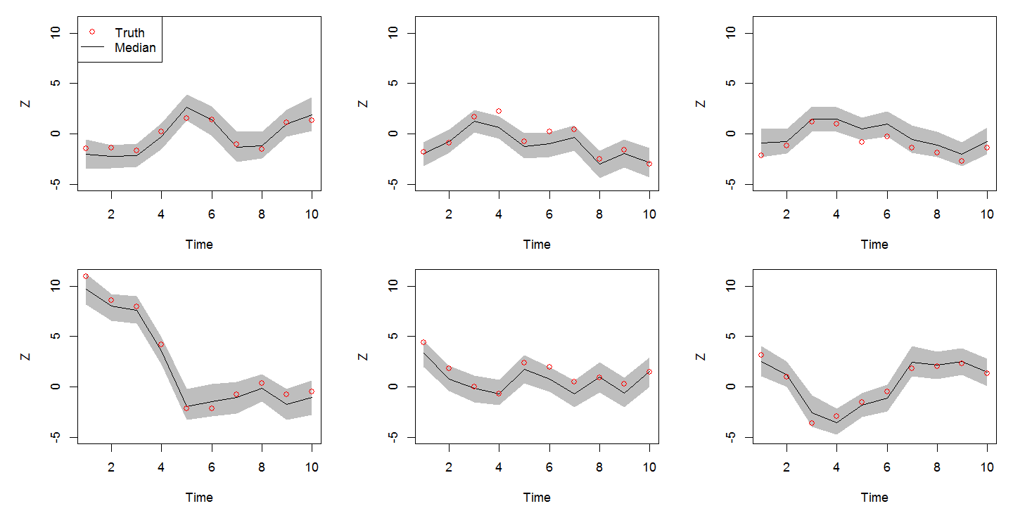
Figure 1: Selected ${\bf Z}_{ik\cdot}$ curves from one dataset of the first simulation study. Plots in the same row correspond to the same county, and plots in the same column correspond to the same group. Black lines denote posterior medians, red circles denote true values, and gray bands denote the 95% CI.

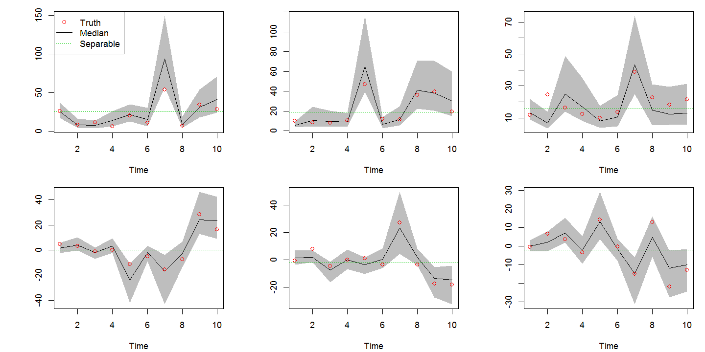
Figure 2: Estimated $G_{t;k,k^{\prime}}$ from one dataset of the first simulation study. Top row displays the diagonal elements, while the bottom row displays the off-diagonal elements. Black lines denote posterior medians, red circles denote true values, and gray bands denote the 95% CI. For comparison purposes, the green lines denote the analogous values from the separable model.

4.2 Varying population sizes

In our second simulation study, we generated data using the same design as described in Section 4.1, but here we assigned $n_{ikt}$ to be the population of the $i$th county at time $t$ for the following subpopulations: white men ($k=1$), white women ($k=2$), and black men and women ($k=3$). While white men and women have $n_{ikt}>200$ in all counties for all time periods, there are many counties with small black population sizes. As such, we combine black men and women to limit the number of counties with no data. In cases where a county has no population during time $t$, however, we assume $n_{ikt}=1$ and treat $Y_{ikt}$ as missing.

Our model was again able to obtain accurate estimates for the $Z_{ikt}$ and the various elements of the $G_{t}$ while outperforming the separable model in all 100 datasets (based on DIC). Furthermore — aside from an expected increase in the width of the credible intervals — there does not appear to be any degradation in the estimation for these parameters as we shift from the well-populated groups to the third, less populated group. Unfortunately, our model again performs less well with respect to the temporal correlation parameters, $\rho_{k}$. It is understandable, though, how the problem from our first example would be exacerbated here, as the amount of information provided by each group depends on the county populations.

4.3 General findings

In both simulation studies, the MSTCAR was able to obtain accurate estimates of both the $Z_{ikt}$ and the $G_{t}$. While the nonseparable model offered improved DIC when compared to the separable model, it is important to note that the differences were not substantial, with just over a 1% reduction on average. This suggests that the key benefit of the MSTCAR model (with respect to model fit) is that it provides more precise results (i.e., narrower credible intervals) than the separable model while still achieving the desired coverage.

Based on these results, the $\rho_{k}$ parameters appear to be difficult to identify. As such, if inference on the $\rho_{k}$ is desired, it may be necessary to run our MCMC algorithms for more iterations and consider thinning our samples to obtain samples which are less correlated over the course of the chain. Another option would be to consider respecifying our priors for the $\rho_{k}$. In these simulation studies, we had assumed a $\mbox{$\text{Beta}$}(9,1)$ prior for $\rho_{k}$, but a more informative prior may be appropriate, particularly in the case of varying population sizes. For instance, we could assume a multi-level model of the form $\rho_{k}\sim\mbox{$\text{Beta}$}\left(\upsilon_{\rho}\rho_{0},\upsilon_{\rho}(1-\rho_{0})\right)$ for $k=1,\ldots,N_{g}$, where $\rho_{0}\sim\mbox{$\text{Beta}$}\left(a_{0},b_{0}\right)$ and $\upsilon_{\rho}$ is a parameter which controls the informativeness of the prior. In extreme cases, we may even consider forcing $\rho_{k}\equiv\rho_{0}$, which can be induced by letting $\upsilon_{\rho}\to\infty$. In addition to improving the convergence of our MCMC algorithm, this may also lead to minor computational benefits while still yielding a model that is more flexible than the separable model in (8).

5 Analysis of Heart Disease Death Rates

We fitted the nonseparable hierarchical model in (3.3) to the heart disease mortality data described in Section 2 using covariates consisting of only an intercept term for each combination of 2-year time-interval and race/gender (as required, per Besag and Kooperberg,, 1995), forcing the random effects to account for a substantial amount of the spatio-temporal variability in the data. We place a $\mbox{$\text{Beta}$}(9,1)$ prior on each of the $\rho_{k}$ to encourage higher temporal correlations in the model, and we use a vague inverse Wishart prior for each of the $G_{t}$. We ran the MCMC algorithm with a single chain for 6,000 iterations, diagnosing convergence via trace plots for many of the model parameters and discarding the first 1,000 iterations as burn-in. Following that, we thinned our posterior samples by removing 9 out of 10 samples — while this is not theoretically necessary, it reduced the burden of storing excess samples for our over 200,000 random effects. Estimates provided are based on posterior medians, and 95% credible intervals (95% CI) were obtained by taking the 2.5- and 97.5-percentiles from the thinned post-burn-in samples. To determine if the burden associated with fitting this nonseparable model was necessary, we compared our model to the separable model in (8) and the $N_{g}$ independent STCAR models in (7).

Table 1 displays the results of our model comparison. Here, it is clear that the independent STCAR models — while computationally convenient — are inadequate for these data, as both the separable and MSTCAR models offer improvements in DIC of over 94,000 units. As seen in Section 4, the separable and MSTCAR models appear to perform similarly, with the MSTCAR model having a DIC only 5,828 units lower. Given the evidence in the literature that DIC tends to favor over-fitted models (e.g., Robert and Titterington,, 2002), it remains unclear if the flexibility of the MSTCAR model is required here; nevertheless, we will henceforth focus our attention on results from the MSTCAR model.

Model	DIC	$p_{D}$
STCAR	2,423,049	32,110
Separable	2,334,355	24,185
MSTCAR	2,328,527	25,699

Table 1: Model fit comparison between the independent STCAR models, a separable model, and the nonseparable MSTCAR model proposed here. Lower values of DIC indicate a better compromise of model fit and model complexity, where $p_{D}$ is a measure of model complexity.

Figure 3 displays the expected nationwide death rate trends for each group. These trend lines were computed by first computing the posterior distribution for the expected value for $Y_{ikt}$ as $\widehat{Y}_{ikt}={\bf x}_{ikt}^{\prime}\boldsymbol{\beta}_{k}+Z_{ikt}$. We then estimated the nationwide death rate for group $k$ at time $t$ by constructing the posterior for

$$\widehat{Y}_{\cdot kt}=\frac{\sum_{i}\widehat{Y}_{ikt}n_{ikt}}{\sum_{i}n_{ikt}}.$$

A number of important findings can be found from this figure. First and foremost, all four of our race/gender groups have experienced substantial declines, with death rates being more than cut in half. Secondly, men of both races experience significantly higher rate of heart disease-related death than women. That said, men and women of both races do not decline at the same rate; e.g., while white men began the study as the population with the highest risk, they were soon surpassed by black men, whose rates appear to be relatively stagnant for the period from 1975–76 to 1987–88. This trend is also visible for black women.

To illustrate the changing geographic patterns, Figure 4 displays heart disease death rates for white men for four time-intervals. Here, we notice an interesting trend, as several major cities (e.g., Denver, CO; Washington, DC; Atlanta, GA; Minneapolis, MN) are consistently leading the charge toward lower rates of heart disease related death for white men in their respective regions. On the other hand, there are collections of counties in which rates are lagging behind, most prominently along the southern Mississippi River and much of the Deep South. Similar patterns can be found for the remaining race/gender groups.

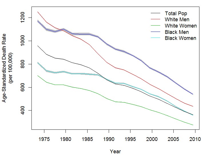
Figure 3: Heart disease death rates over time for each of the race/gender groups compared to the total population. Gray bands denote the 95% credible intervals for the estimates.

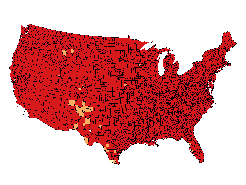
(a) 1973–74

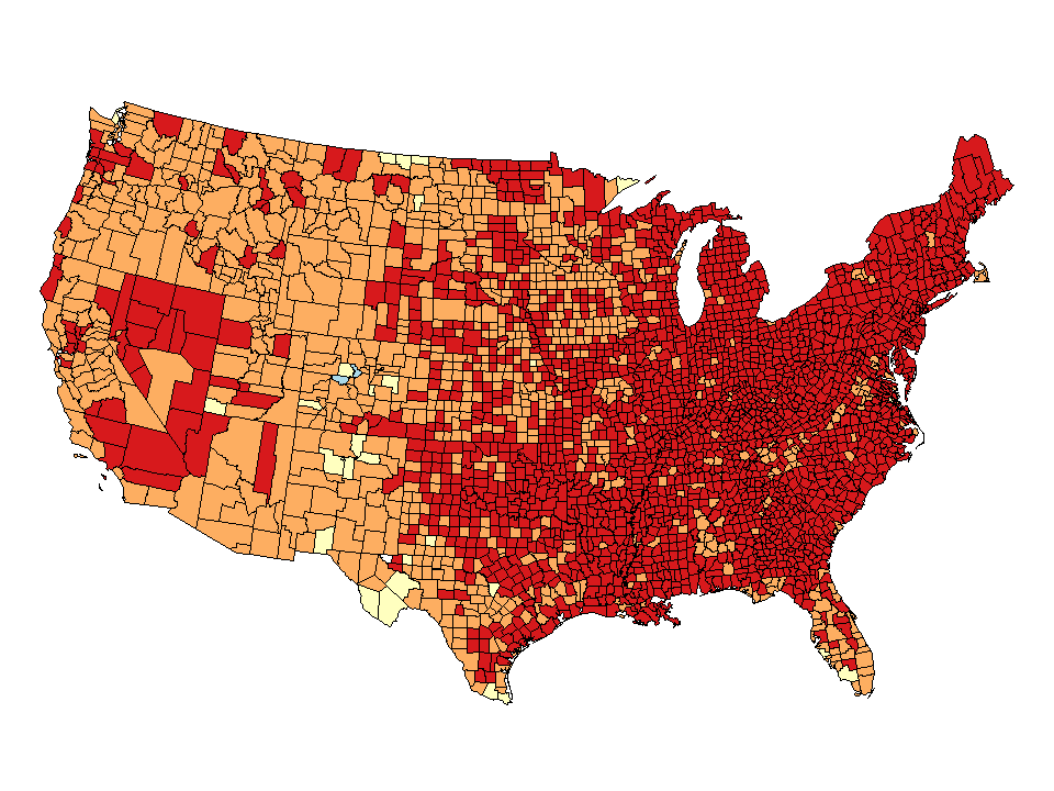
(b) 1985–86

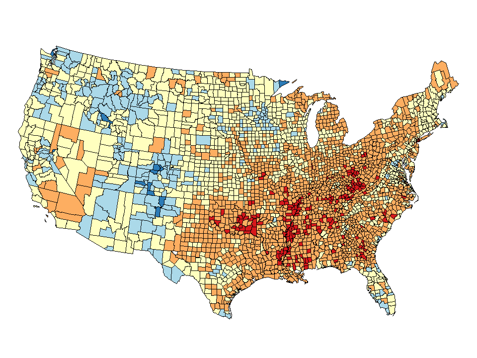
(c) 1997–98

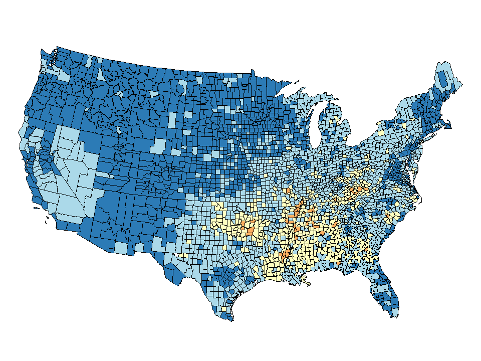
(d) 2009–10

Figure 4: Estimated expected heart disease death rates (per 100,000) for white men for selected time-intervals.

We now turn our attention to the numerous variance parameters permitted by the use of the nonseparable model. While in Section 4 we presented posterior distributions for the elements of $G_{t}$ (Figure 2), these parameters are not necessarily of direct interest as they are the variance parameters for ${\bf v}_{\ell\cdot t}$, and thus they are not directly interpretable on the scale of the data. Instead, we need to use our posterior samples of $G_{t}$ and $\rho_{k}$ to construct $\mbox{$\Sigma$}_{\eta}$ from (10). These values coincide to the conditional covariance matrix of ${\bf Z}_{i\cdot\cdot}$ (when scaled by the number of neighbors, $m_{i}$), and thus are interpretable on the scale of the data. Figure 5 displays the diagonal elements of $\mbox{$\Sigma$}_{\eta}$ from the nonseparable model, as compared to the analogous estimates from the separable model. Here, we find — for all race/gender groups — that the variability of $Z_{ikt}$ has decreased substantially from the beginning of the study period to the end. More importantly, however, we note that the separable model severely underestimates the variance at the beginning of the study and severely overestimates the variance at the end. As shown in Figure B.2 of the Web Appendix, this can lead to oversmoothing when the rates are the highest (the 1970s) and undersmoothing when the rates are lowest (the 2000s), neither of which is desirable. This may be due to the fact that the rates themselves decline over time. Correlations between race/gender groups are all non-zero, with high correlations between genders of the same race and moderate correlations between races; these results can be found in Figure B.3 of the Web Appendix.

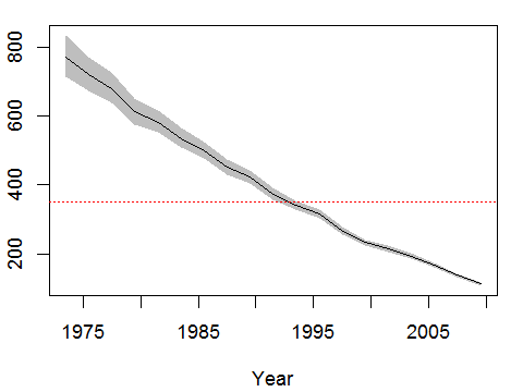
(a) White Men

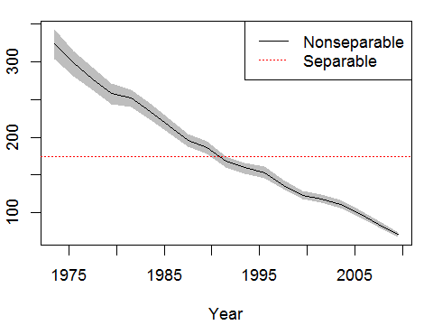
(b) White Women

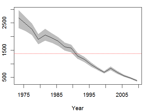
(c) Black Men

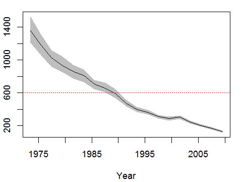
(d) Black Women

Figure 5: Estimated diagonal elements of $\mbox{$\Sigma$}_{\eta}$ for the heart disease mortality data for our four race/gender groups. Black lines denote posterior medians from the nonseparable model while gray bands denote 95% CI. For comparison purposes, the red line indicates the analogous value from the separable model which is constant over time.

6 Discussion

In this paper, we have proposed a nonseparable framework for the purpose of modeling a dataset comprised of temporally-varying county-level heart disease death rates for multiple race/gender populations. We evaluated the validity of the proposed methodology — referred to as the MSTCAR model — via simulation and demonstrated that the model was capable of providing a good fit to the data and obtaining accurate estimates for the many variance parameters. Not only did the MSTCAR model outperform two more conventional models, but we show our model can help control the degree of smoothing in data which undergo a substantial temporal evolution during the study period.

While the methods proposed here are much more sophisticated than more commonplace models like those discussed in Section 3.2, there are a number of extensions which could be used to enhance the MSTCAR model. For manageable values of $N_{s}$, for instance, one could envision models with region-specific parameters $G_{it}$ and $\rho_{ik}$. Implementing these models would likely require the use of a proper CAR model (e.g., the model proposed in Section 3 is constructed using only $N_{s}-1$ latent vectors), say by replacing $(D-W)$ in (12) with $(D-\alpha_{kt}W)$, where $\alpha_{kt}\in[0,1)$ ensures propriety and $\alpha_{kt}=1$ yields the improper CAR-based model used here. Furthermore, one may choose to use a multi-level modeling approach for specifying priors for many of these parameters, such as

$$G_{it}\sim\mbox{$\text{InvWish}$}\left(\nu_{i}G_{t},\nu_{i}\right),\;G_{t}\sim\mbox{$\text{Wish}$}\left(1/\nu G_{0},\nu\right),\;\text{and}\;G_{0} \sim\mbox{$\text{InvWish}$}\left(\nu_{0}G,\nu_{0}\right)$$

to facilitate additional borrowing-of-strength. Computational burden and identifiability concerns notwithstanding, such a model would be rather intuitive to specify and construct; i.e., one could let $\mbox{\boldmath$\eta$}_{i\cdot\cdot}\sim N\left(\textbf{0},\mbox{$\Sigma$}_{\eta_{i}}\right)$, where $\mbox{$\Sigma$}_{\eta_{i}}$ is constructed as in (10) with $i$ subscripts. Based on the results of Quick et al., (2015) — where the authors extended a separable space-time model to allow for region-specific variance parameters — there is evidence to believe that models of this sort may offer substantial improvements in fit.

For cases where $N_{s}$ is large, one may also consider using dimension reduction techniques such as those proposed by Hughes and Haran, (2013) and extended by Bradley et al., (2014). Unfortunately, it’s unclear whether or not this would actually result in computational gains in our setting without making additional assumptions, as the approach of Hughes and Haran, (2013) removes the conditional properties which make CAR models attractive. That is, when implementing the MSTCAR model proposed here, one need only invert and manipulate matrices of rank $N_{g}N_{t}$ to sample the ${\bf Z}_{i\cdot\cdot}$, albeit this requires looping through each of the $N_{s}$ areal regions. An analogous approach based on Hughes and Haran, (2013), however, would replace this $N_{s}$ loop with a single $N_{s}^{*}N_{g}N_{t}$-dimensional update, where $N_{s}^{*}\ll N_{s}$ is the rank of the reduced spatial domain. Were we to reduce the dimension of our spatial domain from $N_{s}=3,099$ to $N_{s}^{*}=310$ (a 90% reduction), this would still require manipulating matrices of rank $N_{s}^{*}N_{g}N_{t}=23,560$, which would not be feasible in our setting. While one could take advantage of the AR(1) structure to ease the burden, this would result in the manipulation of matrices of rank $N_{s}^{*}N_{g}$, which may still be too large to implement in practice without resorting to the shared component model of Bradley et al., (2014).

In the immediate future, we have two primary areas for next steps. Motivated by this and earlier work, we aim to investigate the observed geographic disparities in heart disease death rates by identifying potential factors which may be associated with the patterns observed here. In addition to further exploring the mechanics driving heart disease death rates, we plan to apply a similar modeling framework to data comprised of county-level stroke-related death rates. As stroke data are typically more erratic with much lower rates of incidence, these data will present additional challenges. In particular, the normal approximation used in this analysis will be less appropriate; as such, we aim to explore the possibility of implementing this methodology in a log-linear modeling framework using a Poisson likelihood.

References

- Anderson et al., (2001) Anderson, R. N., Miniño, A. M., Hoyert, D. L., and Rosenberg, H. M. (2001). “Comparability of cause of death between ICD–9 and ICD–10: Preliminary Estimates.” National Vital Statistics Reports, 49.
- Banerjee et al., (2014) Banerjee, S., Carlin, B. P., and Gelfand, A. E. (2014). Hierarchical Modeling and Analysis of Spatial Data. Chapman & Hall/CRC.
- Besag, (1974) Besag, J. (1974). “Spatial interaction and the statistical analysis of lattice systems (with Discussion).” Journal of the Royal Statistical Society, Series B, 36, 192–236.
- Besag et al., (1995) Besag, J., Green, P., Higdon, D., and Mengersen, K. (1995). “Bayesian computation and stochastic systems (with discussion).” Statistical Science, 10, 3–66.
- Besag and Kooperberg, (1995) Besag, J. and Kooperberg, C. (1995). “On conditional and intrinsic autoregressions.” Biometrika, 82, 733–746.
- Besag et al., (1991) Besag, J., York, J., and Mollié, A. (1991). “Bayesian image restoration, with two applications in spatial statistics.” Annals of the Institute of Statistical Mathematics, 43, 1–59.
- Bradley et al., (2014) Bradley, J. R., Wikle, C. K., and Holan, S. H. (2014). “Mixed effects modeling for areal data that exhibit multivariate-spatio-temporal dependencies.” ArXiv preprint, arXiv:1407.7479.
- Carlin and Banerjee, (2003) Carlin, B. P. and Banerjee, S. (2003). “Hierarchical multivariate CAR models for spatio-temporally correlated survival data (with discussion).” In Bayesian Statistics 7, eds. J. M. Bernardo, M. J. Bayarri, J. O. Berger, A. P. Dawid, D. Heckerman, A. F. M. Smith, and M. West, 45–63. Oxford: Oxford University Press.
- Casper et al., (2015) Casper, M., Kramer, M., Quick, H., Greer, S., Schieb, L., and Vaughan, A. (2015). “Changes in the geographic pattern of heart disease mortality in the United States, 1973–2010.” Submitted to Circulation.
- Congdon, (2002) Congdon, P. (2002). “A multivariate model for spatio-temporal health outcomes with an application to suicide mortality.” Geographical Analysis, 36, 235–258.
- Cressie and Wikle, (2011) Cressie, N. and Wikle, C. K. (2011). Statistics for Spatio-Temporal Data. Hoboken, NJ: Wiley.
- Daniels et al., (2006) Daniels, M., Zhou, Z., and Zhou, H. (2006). “Conditionally specified spacetime models for multivariate processes.” Journal of Computational and Graphical Statistics, 15, 157–177.
- Ford and Capewell, (2011) Ford, E. S. and Capewell, S. (2011). “Proportion of the decline in cardiovascular mortality disease due to prevention versus treatment: public health versus clinical care.” Annual Review of Public Health, 32, 5–22.
- Fridley and Dixon, (2007) Fridley, B. L. and Dixon, P. (2007). “Data augmentation for a Bayesian spatial model involving censored observations.” Environmetrics, 18, 107–123.
- Gelfand et al., (1998) Gelfand, A. E., Ghosh, S. K., Knight, J. R., and Sirmans, C. F. (1998). “Spatio-temporal modeling of residential sales data.” Journal of Business and Economic Statistics, 16, 312–321.
- Gelfand and Vounatsou, (2003) Gelfand, A. E. and Vounatsou, P. (2003). “Proper multivariate conditional autoregressive models for spatial data analysis.” Biostatistics, 4, 11–25.
- Gelman, (2006) Gelman, A. (2006). “Prior distributions for variance parameters in hierarchical models.” Bayesian Analysis, 1, 515–533.
- Gillum et al., (2012) Gillum, R. F., Mehari, A., Curry, B., and Obisesan, T. O. (2012). “Racial and geographic variation in coronary heart disease mortality trends.” BMC Public Health, 12, 410.
- Greenlund et al., (2007) Greenlund, K. J., Giles, W. H., Keenan, N. L., Malarcher, A. M., Zheng, Z. J., Casper, M. L., and Croft, J. B. (2007). “Heart disease and stroke mortality in the twentieth century.” In Silent victories: the history and practice of public health in twentieth-century America, eds. J. W. Ward and C. Warren, 381–400. Oxford: Oxford University Press.
- Hodges et al., (2003) Hodges, J. S., Carlin, B. P., and Fan, Q. (2003). “On the precision of the conditionally autoregressive prior in spatial models.” Biometrics, 59, 317–322.
- Hughes and Haran, (2013) Hughes, J. and Haran, M. (2013). “Dimension reduction and alleviation of confounding for spatial generalized linear mixed models.” Journal of the Royal Statistical Society, Series B, 75, 139–159.
- Klebba and Scott, (1980) Klebba, A. J. and Scott, J. H. (1980). “Estimates of selected comparability ratios based on dual coding of 1976 death certificates by the eighth and ninth revisions of the International Classification of Diseases.” National Vital Statistics Reports, 28.
- Knorr-Held, (2000) Knorr-Held, L. (2000). “Bayesian modelling of inseparable space-time variation in disease risk.” Statistics in Medicine, 19, 2555–2567.
- Knorr-Held, (2002) — (2002). “Some remarks on Gaussian Markov random field models for disease mapping.” In Highly Structured Stochastic Systems, eds. P. Green, N. Hjort, and S. Richardson, 260–264. Oxford: Oxford University Press.
- Knorr-Held and Besag, (1998) Knorr-Held, L. and Besag, J. (1998). “Modelling risk from a disease in time and space.” Statistics in Medicine, 17, 2045–2060.
- Knorr-Held and Best, (2001) Knorr-Held, L. and Best, N. (2001). “A shared component model for detecting joint and selective clustering of two diseases.” Journal of the Royal Statistical Society, Series A, 164, 73–85.
- Kramer et al., (2015) Kramer, M. R., Valderrama, A. L., and Casper, M. (2015). “Decomposing black-white disparities in heart disease mortality in the U.S., 1973–2010: an age-period-cohort analysis.” American Journal of Epidemiology. To appear.
- Murphy et al., (2013) Murphy, S. L., Xu, J., and Kochanek, K. D. (2013). “Deaths: final data for 2010.” National Vital Statistics Reports, 61, 4.
- NCHS, (2013) NCHS (2013). “Bridged-race population estimates: United States July 1st resident population by state, county, age, sex, bridged-race, and Hispanic origin.” Available from http://www.cdc.gov/NCHS/nvss/bridged_race.htm.
- Quick et al., (2013) Quick, H., Banerjee, S., and Carlin, B. P. (2013). “Modeling temporal gradients in regionally aggregated California asthma hospitalization data.” Annals of Applied Statistics, 7, 154–176.
- Quick et al., (2015) Quick, H., Carlin, B. P., and Banerjee, S. (2015). “Heteroscedastic CAR models for areally referenced temporal processes for analyzing California asthma hospitalization data.” Journal of the Royal Statistical Society, Series C. doi: 10.1111/rssc.12106.
- Robert and Titterington, (2002) Robert, C. P. and Titterington, D. M. (2002). “Discussion of a paper by D. J. Spiegelhalter et al.” Journal of the Royal Statistical Society, Series B, 64, 621–622.
- Rue and Held, (2005) Rue, H. and Held, L. (2005). Gaussian Markov Random Fields. Chapman & Hall/CRC.
- Sempos et al., (1988) Sempos, C., Cooper, R., Kovar, M. G., and McMillen, M. (1988). “Divergence of the recent trends in coronary mortality for the four major race-sex groups in the United States.” American Journal of Public Health, 78, 1422–1427.
- Spiegelhalter et al., (2002) Spiegelhalter, D. J., Best, N., Carlin, B. P., and van der Linde, A. (2002). “Bayesian measures of model complexity and fit (with discussion).” Journal of the Royal Statistical Society, Series B, 64, 583–639.
- Stein, (2005) Stein, M. L. (2005). “Space-time covariance functions.” Journal of the American Statistical Association, 100, 310–321.
- Tzala and Best, (2008) Tzala, E. and Best, N. (2008). “Bayesian latent variable modelling of multivariate spatio-temporal variation in cancer mortality.” Statistical Methods in Medical Research, 17, 97–118.
- Vaughan et al., (2014) Vaughan, A. S., Kramer, M. R., and Casper, M. (2014). “Geographic disparities in declining rates of heart disease mortality in the southern United States, 1973–2010.” Preventing Chronic Disease, 11, 140203. http://dx.doi.org/10.5888/pcd11.140203.
- Vaughan et al., (2015) Vaughan, A. S., Kramer, M. R., Waller, L. A., Schieb, L. J., Greer, S., and Casper, M. (2015). “Comparing methods of measuring geographic patterns in temporal trends: an application to county-level heart disease mortality in the United States, 1973 to 2010.” Annals of Epidemiology, 25, 329–335.
- Waller et al., (1997) Waller, L. A., Carlin, B. P., Xia, H., and Gelfand, A. E. (1997). “Hierarchical spatio-temporal mapping of disease rates.” Journal of the American Statistical Association, 92, 607–617.
- Young et al., (2010) Young, F., Capewell, S., Ford, E. S., and Critchley, J. A. (2010). “Coronary mortality declines in the U.S. between 1980 and 2000: quantifying the contribution from primary and secondary prevention.” American Journal of Preventive Medicine, 39, 228–234.
- Zhu et al., (2013) Zhu, L., Waller, L. A., and Ma, J. (2013). “Spatial-temporal disease mapping of illicit drug abuse or dependence in the presence of misaligned ZIP codes.” GeoJournal, 78, 463–474.