Study of decuplet baryon resonances from lattice QCD

Abstract

A lattice QCD study of the strong decay width and coupling constant of decuplet baryons to an octet baryon - pion state is presented. The transfer matrix method is used to obtain the overlap of lattice states with decuplet baryon quantum numbers on the one hand and octet baryon-pion quantum numbers on the other as an approximation to the matrix element of the corresponding transition. By making use of leading order effective field theory, the coupling constants, as well as the widths for the various decay channels are determined. The transitions studied are $\Delta\to\pi\,N$, $\Sigma^{*}\to\Lambda\,\pi$, $\Sigma^{*}\to\Sigma\,\pi$ and $\Xi^{*}\to\Xi\,\pi$. We obtain results for two ensembles of $N_{f}=2+1$ dynamical fermion configurations, one using domain wall valence quarks on a staggered sea at a pion mass of $350\,\mathrm{MeV}$ and a box size of $3.4\,\mathrm{fm}$ and a second one using domain wall sea and valence quarks at pion mass $180\,\mathrm{MeV}$ and box size $4.5\,\mathrm{fm}$.

I Introduction

The study of resonances from first principles using lattice Quantum Chromodynamics (QCD), has progressed significantly. Most of these studies are based on the Lüscher approach Luscher:1985dn ; Luscher:1986pf and extension thereof Rummukainen:1995vs ; Fu:2011xz ; Gockeler:2012yj ; Leskovec:2012gb ; Doring:2012eu that extract scattering lengths and phase shifts from discrete energy levels in a finite volume. The approach has been generalized to the case of coupled channels He:2005ey ; Bernard:2008ax ; Doring:2011nd ; Lang:2011mn ; Briceno:2012yi ; Hansen:2012tf ; Guo:2012hv ; Li:2012bi ; Briceno:2013bda ; Wu:2014vma and three identical boson scattering Briceno:2012rv , and a growing number of studies is being carried out in the meson sector. A pioneering study of meson-baryon and baryon-baryon scattering lengths was already carried out twenty years ago Fukugita:1994ve and more recent studies include those by members of the NPLQCD Briceno:2013hya ; Torok:2009dg and HALQCD Aoki:2011ep collaborations and other groups Lage:2009zv . Despite this progress, the application of the Lüscher approach to baryon resonances has been limited since the method requires very precise data for multiple spatial volumes or various reference frames of different total linear momentum making it computationally very demanding.

Another method to study hadronic resonant decays from lattice QCD was proposed in Refs. McNeile:2002az ; McNeile:2002fh and successfully applied in the study of meson decays Michael:2006hf ; Michael:2005kw . A first application of this transfer matrix method to baryons was carried out in Refs. Alexandrou:2013ata ; Alexandrou:2014qka . The transfer matrix method as applied here allows to extract the width of a resonant hadronic decay, if the resonance width is small as compared to the resonant energy and well-isolated from other decay channels. In such a situation the method allows us to extract the width from one kinematic point and it thus provides currently a computationally feasible calculation of the width in the baryon sector. This calculation can be seen as a first attempt to compute the width of an unstable baryon that allows us to learn about two-particle interpolating fields in the baryon sector and the associated technicalities and gauge noise.

In this approach, one considers a purely hadronic decay of a baryon $B^{*}$ to a two-particle state. In the cases considered in this work, the two-particle state will be a meson $M$ and a baryon $B$, as illustrated diagrammatically in Fig. [1].

Figure 1: Diagram for the transition $B^{*}\leftrightarrow MB$

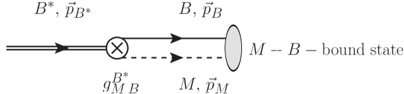
We associate a vertex with the tree-level transition graph in Fig. [1] and the strength of the interaction at the vertex is measured in terms of an effective coupling constant $g^{B^{*}}_{MB}$. We define this coupling to coincide with the coupling that appears in the leading order continuum effective field theory for the interaction term of the hadronic fields $M,\,B$ and $B^{*}$ in the effective Lagrangian. This will be made more explicit later on in connection with Eq.  (10).

In order to study a decay $B^{*}\to M\,B$ in the Euclidean quantum field theory we need to formulate it in terms of energies or hadronic matrix elements. In lattice QCD we use interpolating fields to create states with the quantum of the decuplet baryon $B^{*}$ and the octet baryon $B$ and the meson $M$. We restrict our consideration to the two lowest-lying states with the desired quantum numbers, which we label by $|\,B^{*}\rangle$ and $|\,MB\rangle$. If $B^{*}$ does not decay then its overlap with $|\,MB\rangle$ is zero and it is an asymptotic state of the theory. These states can then be thought off as the eigenstates of a non-interacting lattice transfer matrix $\hat{\mathrm{T}}^{0}$ defined by a Hamiltonian $\hat{\mathrm{H}}_{0}=|B^{*}\rangle\langle B^{*}|+|\,MB\rangle\langle\,MB|$. Our approach here is to study the overlap of the states created by the interpolating fields $B^{*}$ and $M\,B$ for the case where the energy levels of these states are near-degenerate. The interaction Hamiltonian to leading order in the perturbation will then be given by $\hat{\mathrm{H}}=\hat{\mathrm{H}}_{0}+|B^{*}\rangle\langle MB|+|\,MB\rangle\langle\,B^{*}|$.

The off-diagonal elements of the Hamiltonian will be the overlap $\langle B^{*}\,|\,\hat{\mathrm{H}}\,|\,MB\rangle$. Thus our assumption is that a state $|\,B^{*}\rangle$ created initially at time $t_{i}$ propagates in Euclidean time on the lattice to final time $t_{f}$, makes one transition to $|\,MB\rangle$ at any intermediate time step $t\to t+a$ on the lattice. If the (real valued) lattice transition amplitude is small in terms of the inverse propagation time $\left(t_{f}-t_{i}\right)^{-1}$ and if the energy gap between the states $|\,B^{*}\rangle$ and $|\,MB\rangle$ is sufficiently small then one can evaluate the overlap and relate it to the coupling constant and then to the decay width McNeile:2002fh . We stress that the propagator of the state $B^{*}$ is fully dressed and so is the propagator of the $M\,B$ state including interactions between the two particles. A tree-level effective interaction Lagrangian can be written in terms of the fields $B^{*},B$ and $M$ Pascalutsa:2002pi with coupling constant $g^{B^{*}}_{MB}$, which is related to the overlap $\langle B^{*}\,|\,\hat{\mathrm{H}}\,|\,MB\rangle$ as will be discussed in section II.

In order compute the overlap of these states we need to choose ensembles for which the energy gap $\delta=E_{B^{*}}-E_{MB}$ is small in units of the inverse propagation time from initial to final state $\delta\ll 1/(t_{f}-t_{i})$. Since on a finite lattice the allowed momenta are discretized the energies will not in general match. Thus, this condition will be only approximately satisfied for the ensembles we have at our disposal. A second condition that is required is that the propagation time $t_{f}-t_{i}$ is sufficiently large compared to the energy difference between the ground state energy of $B^{*}$ and its first excited state as well as between the lowest energy of the $B\,M$ system and its excited state with the same quantum numbers so that only the two lowest-lying states of interest dominate in the transition matrix element. The extraction of the overlap from lattice measurements is detailed in section II. The transition matrix element $\mathcal{M}(B^{*}\to MB)\propto\langle B^{*}\,|\,H\,|\,MB\rangle$ for the situation in which the energy levels of the two states are degenerate. Using Fermi’s Golden rule one can relate this decay matrix element to the decay width

$$\Gamma^{B^{*}}_{M\,B} =2\pi\,|\mathcal{M}(B^{*}\to MB)|^{2}\,\rho\,,$$ (1)

where $\rho$ is the density of states at the transition energy. As already mentioned, in this study we work to lowest order considering only a single transition amplitude and allowing for large enough time separation $t_{f}-t_{i}$ so only the lowest states in the initial and final states give the dominating contribution. To this order we also neglect further elastic rescattering of $M\,B$ in the final $MB$ state.

In our first study Alexandrou:2013ata , we successfully applied this approach to study the $\Delta$ resonance using a hybrid action with domain wall valence quarks on a staggered sea. Here we extend our study to include the decuplet baryons $\Sigma^{*}$ and $\Xi^{*}$. In addition, we investigate the applicability of All Mode Averaging (AMA) Blum:2012uh in improving the statistical accuracy using the $\Delta$ resonance as test case. In this work we also analyze an ensemble of domain wall fermions (DWF) corresponding to a pion mass of 180 MeVArthur:2012opa for which the energy matching, in particular for the $\Delta$, is very well satisfied. The results based on this ensemble of $N_{f}=2+1$ DWF for the widths of the $\Delta$, the $\Sigma^{*}$ and the $\Xi^{*}$ as well as the results using the hybrid ensemble for the $\Sigma^{*}$ and $\Xi^{*}$ constitute the first determination of the decay widths of these resonances using lattice QCD.

The paper is organized as follows: In section II we present the method and give the technical details. In section III we show our lattice QCD results, in section IV we discuss these results and their relation to the decay widths and in section V we present our conclusions.

II Technical details of the method

The method that we consider in this work was first described in Refs. McNeile:2002az ; McNeile:2002fh ; McNeile:2004rf where it was applied to the study of meson decays. The method was extended for the case of the $\Delta$ resonance and first results were obtained using an ensemble of domain wall valence quarks on an $N_{f}=2+1$ staggered sea, which we will refer to as hybrid approach Alexandrou:2013ata . In this section, we explain the technical steps involved paying particular attention to the description of the decays of decuplet baryons, which is the focus of this work.

II.1 Lattice correlation function and normalization

We consider the following strong decays of a decuplet baryon to a meson-baryon final state:

$$\Delta \to\pi\,N$$

$$\Sigma^{*} \to\pi\,\Sigma\,,\>\pi\,\Lambda$$

$$\Xi^{*} \to\pi\,\Xi\,,$$ (2)

generically denoted by $B^{*}\to M\,B$. Due to the isospin symmetry of the lattice action, we can choose any isospin channel for each case. In this study, we consider the $\Delta^{++}$, the $\Sigma^{*+}$ and the $\Xi^{*-}$ with interpolating fields given by

$$J_{B^{*}}^{\mu\alpha}(t,\vec{P}) =\sum\limits_{\vec{x}}\,J_{B^{*}}^{\mu\alpha}(t,\vec{x})\,\mathrm{e}^{i\vec{P}\vec{x}}$$

$$J_{\Delta^{++}}^{\mu\alpha}(x) =\epsilon_{abc}\,\left(u^{aT}(x)\,C\,\gamma^{\mu}\,u^{b}(x)\right)\,u^{\alpha\,c}(x)$$

$$J_{\Sigma^{*+}}^{\mu\alpha}(x) =\frac{1}{\sqrt{3}}\,\epsilon_{abc}\,\Big{[}\left(u^{aT}(x)\,C\,\gamma^{\mu}\,u^{b}(x)\right)\,s^{\alpha\,c}(x)+2\,\left(s^{aT}(x)\,C\,\gamma^{\mu}\,u^{b}(x)\right)\,u^{\alpha\,c}(x)\Big{]}$$

$$J_{\Xi^{*-}}^{\mu\alpha}(x) =\epsilon_{abc}\,\left(s^{aT}(x)\,C\,\gamma^{\mu}\,d^{b}(x)\right)\,s^{\alpha\,c}(x)\,,$$ (3)

where lower case Latin (Greek) letters denote color (spin) indices and $C=i\gamma_{0}\,\gamma_{2}$ is the charge conjugation matrix.

As interpolating fields for the meson-baryon states we take the product of the interpolating fields of the corresponding meson and baryon:

$$J_{MB}^{\alpha}(t,\vec{p}_{M},\vec{p}_{B}) =\sum\limits_{\vec{y},\vec{z}}\,J_{M}(t,\vec{y})\,J_{B}^{\alpha}(t,\vec{z})\,\mathrm{e}^{i(\vec{p}_{M}\vec{y}+\vec{p}_{B}\vec{z})}$$

$$J_{\pi^{+}}(y) =\bar{d}(y)\,\gamma_{5}\,u(y)$$

$$J_{N}^{\alpha}(z) =\epsilon_{abc}\,\left(u^{aT}(z)\,C\,\gamma_{5}\,d^{b}(z)\right)\,u^{\alpha\,c}(z)$$

$$J_{\Lambda}^{\alpha}(z) =\frac{1}{\sqrt{6}}\,\epsilon_{abc}\,\Big{[}2\,\left(u^{aT}(z)\,C\,\gamma_{5}\,d^{b}(z)\right)\,s^{\alpha\,c}(z)$$

$$\quad+\left(u^{aT}(z)\,C\,\gamma_{5}\,s^{b}(z)\right)\,d^{\alpha\,c}(z)-\left(d^{aT}(z)\,C\,\gamma_{5}\,s^{b}(z)\right)\,u^{\alpha\,c}(z)\Big{]}$$

$$J_{\Sigma^{0}}^{\alpha}(z) =\frac{1}{\sqrt{2}}\,\epsilon_{abc}\,\Big{[}\left(u^{aT}(z)\,C\,\gamma_{5}\,s^{b}(z)\right)\,d^{\alpha\,c}(z)+\left(d^{aT}(z)\,C\,\gamma_{5}\,s^{b}(z)\right)\,u^{\alpha\,c}(z)\Big{]}$$

$$J_{\Xi^{0}} =\epsilon_{abc}\,\left(s^{Ta}(z)\,C\,\gamma_{5}\,u^{b}(z)\right)\,s^{\alpha\,c}(z)\,.$$ (4)

Previous studies have shown that the two-hadron interpolating fields given in Eq. (4) will primarily overlap with two-hadron states Dudek:2012xn , while the single-hadron interpolating fields in Eq. (3) will have a dominant overlap with single-hadron states.

In the following, we consider kinematics where the total momentum is zero, so in the first line of Eq. (3) we set $\vec{P}=0$ and $\vec{p}_{M}=-\vec{p}_{B}$ in Eq. (4). Using these interpolating fields we build the two-point correlation functions for $C_{B^{*}-B^{*}}$, $C_{B^{*}-MB}$ and $C_{MB-MB}$ as follows:

$$C_{B^{*}-B^{*}}(t_{f}-t_{i}) =\mathrm{Tr}\left(\frac{1}{4}(\mathbb{1}+\gamma_{0})\,P^{3/2}_{kl}\,\sum\limits_{\vec{x}}\,\langle J^{l}_{B^{*}}(t_{f},\vec{x})\,\bar{J}_{B^{*}}^{k}(t_{i},\vec{z})\rangle\right)$$ (5)

$$C_{B^{*}-MB}^{k}(t_{f}-t_{i},\vec{q}) =\mathrm{Tr}\left(\frac{1}{4}(\mathbb{1}+\gamma_{0})\,P^{3/2}_{kl}\,\sum\limits_{\vec{x},\vec{y}}\,\langle J^{l}_{B^{*}}(t_{f},\vec{x})\,J^{\dagger}_{M}(t_{i},\vec{y})\,\bar{J}_{B}(t_{i},\vec{z})\rangle\right)\,\mathrm{e}^{-i\vec{q}(\vec{y}-\vec{z})}$$ (6)

$$C_{MB-MB}(t_{f}-t_{i},\vec{k}_{f},\vec{k}_{i}) =\mathrm{Tr}\left(\frac{1}{4}(\mathbb{1}+\gamma_{0})\,\sum\limits_{\vec{x},\vec{y},\vec{y}^{\prime}}\,\langle J_{B}(t_{f},\vec{x})\,J_{M}(t_{f},\vec{y})\,J^{\dagger}_{M}(t_{i},\vec{y}^{\prime})\,\bar{J}_{B}(t_{i},\vec{z})\rangle\,\right)$$

$$\qquad\times\mathrm{e}^{i\vec{k}_{f}(\vec{y}-\vec{x})-i\vec{k}_{i}(\vec{y}^{\prime}-\vec{z})}$$ (7)

with a fixed source location $(t_{i},\,\vec{z})$. All correlators are defined to include a parity projection $\frac{1}{4}\,\left(\mathbb{1}\pm\gamma_{0}\right)$. In addition, $C_{B^{*}-B^{*}}$ and $C_{B^{*}-MB}$ include a projector to spin 3/2, which at zero total momentum is given by

$$P^{3/2}_{ik} =\delta_{ik}\,\mathbb{1}-\frac{1}{3}\,\gamma_{i}\,\gamma_{k}\,,\quad i,k=1,2,3\,.$$ (8)

To cancel the unknown overlaps of the interpolating fields with the states we construct the ratio

$$R^{B^{*}}_{MB,\,k}\left(t_{f}-t_{i},\,\vec{q},\,\vec{k}_{f},\,\vec{k}_{i}\right) =\frac{C_{B^{*}-MB}^{k}(t_{f}-t_{i},\vec{q})}{\sqrt{C_{B^{*}-B^{*}}(t_{f}-t_{i})\times C_{MB-MB}(t_{f}-t_{i},\vec{k}_{f},\vec{k}_{i})}}\,.$$ (9)

In this work we always consider the case $\vec{k}_{f}=\vec{k}_{i}$ and $|\vec{q}|=|\vec{k}_{f}|$. The 2-point function $C_{MB-MB}$ then only depends on $|\vec{k}_{f}|$ and the ratio can be characterized by a single vector $\vec{k}=\vec{q}$ as $R^{B^{*}}_{MB,\,k}=R^{B^{*}}_{MB,\,k}(t_{f}-t_{i},\vec{k})$

Alignment and polarization for $B^{*}-MB$, momentum averages and angular momentum:

Within leading order in effective field theory, a non-vanishing signal in $C_{B^{*}-MB}^{k}(t,\vec{q})$ only arises when the relative momentum vector is aligned or anti-aligned with the spin projection appearing in the correlation function, i.e. when $\vec{q}\cdot\vec{e}_{k}\neq 0$, where $\vec{e}_{k}$ denotes the unit vector in the $k-$direction. The vertex for the fields $B^{*},\,M,\,B$ in the effective Lagrangian following our notation is given by

$$\mathcal{L}_{I}\sim g^{B^{*}}_{MB}\,\bar{B}^{*}_{\mu}\,\partial_{\mu}\,M^{a}\,T^{a}\,B$$ (10)

with matrices $T^{a}$, which contain the Clebsch-Gordan coefficients for coupling isospin channels.

$$\left(T^{a}\right)_{ik} =\langle I_{B^{*}}=3/2,\,I_{B^{*}}^{3}=i\,|\,I_{B}=1/2,\,I_{B}^{3}=k;\,I_{M}=1,\,I_{M}^{3}=a\rangle\,,$$

$$i\, \in\,\{-3/2,\,-1/2,\,+1/2,\,+3/2\}\,,\quad k\,\in\,\{-1/2,\,+1/2\}\,,\quad a\,\in\,\{-1,0,1\}\,.$$

We perform our calculations with one unit of relative momentum, $|\vec{q}|=2\pi/L$, such that $\vec{q}=(\pm 1,0,0)\,2\pi/L$ or a permutation thereof and thus look at the six combinations $C_{B^{*}-MB}^{k}(t,\pm 2\pi/L\,\vec{e}_{k}),\,k=1,2,3$.

The $B^{*}-MB$ correlator is projected to its spin-3/2 component with $P^{3/2}$. Moreover, the average over positive and negative momentum effectively means that for the $MB$ state we use the interpolating field in its center-of-mass frame

$$J_{MB}^{i}\left(t,\vec{P}=0,k=2\pi/L\right) =\frac{1}{2}\,\sum\limits_{i^{\prime}=1,2,3}\,P^{3/2}_{ii^{\prime}}\,\left[J_{MB}\left(t,\vec{P}=0,k\vec{e}_{i^{\prime}}\right)-J_{MB}\left(t,\vec{P}=0,-k\vec{e}_{i^{\prime}}\right)\right]\,.$$ (11)

In a partial wave expansion, we find that the dominant state excited by the interpolating field given in Eq. (11) will have orbital angular $l=1$. The coupling of the $l=1$ to the nucleon state with spin 1/2 are projected to the component with total angular momentum 3/2. Thus the operators in Eq. (11) and the projected operators in Eq. (3) transform under the spin-3/2 representation of the Lorentz group in the continuum, which is subduced into irreducible representation $\Lambda^{P}=H^{+}$ (positive parity) of the double cover $O^{D}$ of the octahedral group on the lattice (Table III in Ref. Basak:2005ir ). The irreducible representation $H$ contains an overlap with higher partial waves. What simplifies the calculation at hand, is that we only consider the ground state at large Euclidean time, in which all channels but the desired one with $l=1,J^{P}=3/2^{+}$ are exponentially suppressed.

All the standard spin-3/2 interpolating fields $J_{B^{*}}$ involve the spin structure $(q^{T}\,C\,\gamma_{k}\,q)\,q$ and the parity operation in the center-of-mass frame acts as

$$\mathrm{P} :\,J_{B^{*}}^{k}(t,\vec{P}=0)\to\gamma_{0}\,J^{k}_{B^{*}}(t,\vec{P}=0)\,.$$ (12)

The spin-3/2 projector, $P^{3/2}$, and the projector to the component with definite parity commute, such that we have the trivial action

$$\mathrm{P} :\,\frac{1}{4}(1+\gamma_{0})\,P^{3/2}_{kk^{\prime}}\,J_{B^{*}}^{k^{\prime}}(t,\vec{P}=0)\to\frac{1}{4}(1+\gamma_{0})\,P^{3/2}_{kk^{\prime}}\,J_{B^{*}}^{k^{\prime}}(t,\vec{P}=0)\,.$$ (13)

On the other hand, for the $MB-$state with the pseudoscalar meson field we have in the center-of-mass frame and with relative momentum $\vec{k}$

$$\mathrm{P} :\,\frac{1}{4}(1+\gamma_{0})\,J_{MB}(t,\vec{P}=0,\vec{k})\to-\frac{1}{4}(1+\gamma_{0})\,J_{MB}(t,\vec{P}=0,-\vec{k})\,.$$ (14)

Since parity is a symmetry of the lattice action and the $B^{*}-B^{*}$ and $MB-MB$ two-point functions are even under parity, we expect the following relation to hold for the ratio

$$R^{B^{*}}_{MB}(t_{t}-t_{i},\vec{k}) =-R^{B^{*}}_{MB}(t_{t}-t_{i},-\vec{k})\,.$$ (15)

Quark-connected and disconnected diagrams:

The Wick contractions for the correlation function $C_{MB-MB}$ can be represented by two types of diagrams, as shown in Fig. [2]: quark-disconnected ($D$, upper right) and quark-connected (lower diagrams $C_{1,2,3}$).

Figure 2: Diagrams representing different types of Wick contractions for $C_{B^{*}-MB}$ (diagram $T$) and $C_{MB-MB}$ (upper right: quark-disconnected $D$, lower: quark-connected $C_{1,2,3}$).

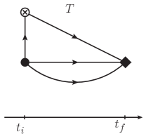
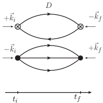
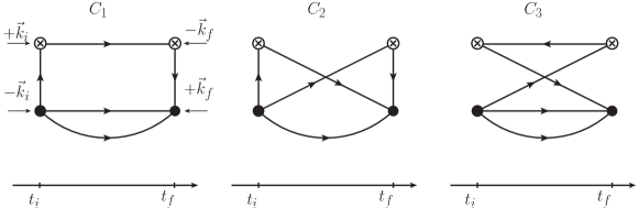
We make two simplifications: i) We neglect the quark-connected diagrams $C_{1}$, $C_{2}$ and $C_{3}$ and ii) approximate the quark-disconnected diagram by the product of expectation values of the individual meson and baryon propagators. This results in a significant reduction in the computational cost. The contractions for diagrams $T$ and $D$, as performed in this work, require one quark propagator and one sequential propagator through the source timeslice $t_{i}$. In contrast, the full contractions for the quark-connected diagrams require all-to-all propagators. We thus set

$$C_{MB-MB}(t_{f}-t_{i},\vec{k}_{f},\vec{k}_{i}) \to C_{MB-MB}(t_{f}-t_{i},\vec{k}_{M},\vec{k}_{B})$$

$$=\langle C_{M-M}(t_{f}-t_{i},\vec{k}_{M})\rangle\times\mathrm{Tr}\left(\frac{1}{4}(1+\gamma_{0})\,\langle C_{B-B}(t_{f}-t_{i},\vec{k}_{B})\rangle\right),$$ (16)

where the meson and baryon propagators are Fourier transformed with independent momenta $\vec{k}_{M}$ and $\vec{k}_{B}$, respectively. In this form the $M-B$ two-point function depends only on the squared momenta $\vec{k}_{M}^{2}$ and $\vec{k}_{B}^{2}$ and for $C_{MB-MB}$ we only use combinations with equal modulus such that we can simply replace the dependence on the pair $(\vec{k}_{M},\vec{k}_{B}))$ by a single vector $\vec{k}$.

Thus, in the asymptotic region of large time separation $(t_{f}-t_{i})/a\gg 1$, we can express this approximation as

$$C_{MB-MB}(t_{f}-t_{i},\vec{k}_{f},\vec{k}_{i}) \overset{(t_{f}-t_{i})/a\gg 1}{\propto}Z_{MB}(\vec{k}_{f},\vec{k}_{i})\,\mathrm{e}^{-E_{MB}(\vec{k}_{f},\vec{k}_{i})(t_{f}-t_{i})}\,u_{MB}(\vec{k}_{f})\,\bar{u}_{MB}(\vec{k}_{i})+\ldots$$

$$\approx Z_{M}(\vec{k}^{2})\,\mathrm{e}^{-E_{M}(\vec{k}^{2})(t_{f}-t_{i})}\,Z_{B}(\vec{k}^{2})\,\mathrm{e}^{-E_{B}(t_{f}-t_{i})}\,u_{B}(\vec{k}_{f})\,\bar{u}_{B}(\vec{k}_{i})+\ldots$$ (17)

II.2 Extraction of coupling and the matrix element

For all baryons $B^{*}$ to $M\,B$ we restrict the lattice Hilbert space to two states $|\,B^{*}\rangle$ and $|\,MB\rangle$ as the dominant baryon and baryon-meson states, respectively Alexandrou:2013ata . In terms of this two-dimensional subspace, the transfer matrix is parametrized as

$$\hat{\mathrm{T}} =\mathrm{e}^{-a\bar{E}}\,\begin{pmatrix}\mathrm{e}^{-a\delta/2}&ax\\ ax&\mathrm{e}^{+a\delta/2}\end{pmatrix}\,.$$ (18)

In accordance with the assumption of a small energy gap we take $\bar{E}=(E_{B^{*}}+E_{MB})/2$ as the mean of the energies of the states and $\delta=E_{MB}-E_{B^{*}}$ as their difference. Fixing an initial and final lattice timeslice $t_{i}$ and $t_{f}$ and summing over all possibilities for a single transition from $B^{*}$ to $MB$, which can occur at any intermediate time-slices between $t_{i}$ and $t_{f}$, it follows that

$$\langle B^{*},\,t_{f}\,|\,MB,\,t_{i}\rangle =\langle B^{*}\,|\,\mathrm{e}^{-H(t_{f}-t_{i})}\,|\,MB\rangle=\langle B^{*}\,|\,\hat{\mathrm{T}}^{n_{fi}}\,|\,MB\rangle$$

$$=\sum\limits_{n=0}^{n_{fi}-1}\,\mathrm{e}^{-(\bar{E}-\delta/2)t_{n}}\,\langle B^{*}\,|\,\hat{\mathrm{T}}\,|\,MB\rangle\,\mathrm{e}^{-(\bar{E}+\delta/2)(\Delta t_{fi}-t_{n}-a)}+\ldots$$

$$=ax\,\frac{\sinh(\delta\,\Delta t_{fi}/2)}{\sinh(a\delta/2)}\,\mathrm{e}^{-\bar{E}\Delta t_{fi}}+\ldots$$ (19)

with $\Delta t_{fi}=t_{f}-t_{i}=an_{fi}$. In Eq. (19) the ellipsis denotes contributions of higher orders in the matrix elements $\langle B^{*}\,|\,\hat{\mathrm{T}}\,|\,MB\rangle$ and $\langle MB\,|\,\hat{\mathrm{T}}\,|\,B^{*}\rangle$, which are at least quadratic in the time separation $\Delta t_{fi}$. As a consequence, by extracting the term linear in $\Delta t_{fi}$ we get the transfer matrix element

$$ax =\langle B^{*}\,|\,T\,|\,MB\rangle\xrightarrow{a\to 0}-a\langle B^{*}\,|\,\mathrm{H}\,|\,MB\rangle\,.$$ (20)

Given the time-dependence of the overlap in Eq. (20), we use two different fit ansätze given by

$$f_{1}(t) =c_{0}+c_{1}\,\sinh\left(c_{2}\,t/(2a)\right)/(c_{2}/2),$$ (21)

$$f_{2}(t) =c_{0}+c_{1}\,\frac{t}{a}+c_{2}\left(\frac{t}{a}\right)^{3}+\ldots$$ (22)

In both cases, we are primarily interested in the parameter $c_{1}$. Although in principle we could take into account the next terms denoted by the ellipsis in Eq. (22), in practice we will not need to go beyond $c_{2}$ to obtain a good fit to the available lattice data with their present accuracy. The parameter $c_{0}$ allows for an offset at $t=0$, which can originate from lattice artifacts or contributions from excited states giving an overlap at zero time, i.e. with no insertion of the transfer matrix. Given that Eq. (19) contains a lattice version of the energy Dirac-$\delta$ function for the finite temporal lattice extent, Eq. (21) allows for fitting the data taking into account a non-zero energy gap. Besides taking into account a finite energy gap, which will be the only contribution to it if the transition happens once in the path integral, the $c_{2}$-term may also effectively be including next-to-leading order contributions arising from overlaps from other intermediate states.

The value of the parameter $c_{2}$ extracted from fitting $f_{1}$ and the one extracted from fitting $f_{2}$ can be related at order $t^{3}$ after expanding $f_{1}$. We indeed find that these two values of the $c_{2}$ parameter show a strong correlation, as expected. Yet in some cases a different value is extracted and hence it is appropriate to use both ansätze to study the systematic uncertainties in the fitting of the lattice QCD data.

As alluded to in Eq. (17), the interpretation of the overlap of lattice states and interpolating fields acting on the vacuum state involves the spinors $u_{B^{*}}$ and $u_{B}$ as follows

$$\sum\limits_{\vec{x}}\,\frac{1}{4}(1+\gamma_{0})\,\langle 0\,|\,J^{\mu\alpha}_{B^{*}}(t,\vec{x})\,\mathrm{e}^{i\vec{P}^{\prime}\vec{x}}\,|\,B^{*},\vec{P},s=3/2,s_{3}\rangle =Z_{B^{*}}(\vec{P}^{2})\,V\,\delta_{\vec{P}\vec{P}^{\prime}}\,u_{B^{*}}^{\mu\alpha}(\vec{P},s_{3})$$ (23)

$$\sum\limits_{\vec{y}}\,\frac{1}{4}(1+\gamma_{0})\,\langle 0\,|\,J_{M}(t,\vec{y})\,J^{\alpha}_{B}(t,\vec{z})\,\mathrm{e}^{i\vec{k}^{\prime}(\vec{y}-\vec{z})}\,|\,MB,\vec{k},s=1/2,s_{3}\rangle =Z_{M}(\vec{k}^{2})\,Z_{B}(\vec{k}^{2})\,V\,\delta_{\vec{k}\vec{k}^{\prime}}\,u_{B}^{\alpha}(-\vec{k},s_{3})\,.$$ (24)

We denote by $s$ the spin quantum number of the baryon fields, $s_{B^{*}}=3/2$ and $s_{B}=1/2$ (having $s_{M}=0$ fixed for the pseudoscalar meson) and by $s_{3}$ its projection to a specific axis. The definition in Eq. (24) assumes that the total linear momentum of the meson-baryon state is zero.

While the ratio $R^{B^{*}}_{MB}$ is constructed such that the numerical factors $Z_{B^{*}/M/B}$ cancel, the spinors remain in the fraction and are combined to spin sums $\Sigma^{B^{*}}_{MB}$ in the numerator and $\Sigma_{B^{*}}$ and $\Sigma_{B}$ in the denominator via summation over the third spin component. To that end, we parametrize the slope $c_{1}=ax$ in Eq. (21), (22) as follows

$$c_{1} =\sum\limits_{\sigma_{3},\tau_{3}}\,\frac{\mathcal{M}(\vec{P}=0,|\vec{k}|,\sigma_{3},\tau_{3})}{\sqrt{N_{B^{*}}\,N_{MB}}}\,V\,\frac{\tilde{\Sigma}^{B^{*}}_{MB}(\vec{P}=0,\vec{k},\sigma_{3}.\tau_{3})}{\sqrt{\Sigma_{B^{*}}(\vec{P}=0)\,\Sigma_{B}(|\vec{k}|)}}$$ (25)

$$\tilde{\Sigma}^{B^{*}}_{MB}(\vec{P}=0,|\vec{k}|,\sigma_{3}) =\frac{1}{6}\,\sum\limits_{j=\pm 1,\pm 2,\pm 3}\,\mathrm{sign}(j)\,\frac{1}{4}(1+\gamma_{0})_{\alpha\beta}\,u^{j\beta}_{B^{*}}(\vec{P}=0,\sigma_{3})\,\bar{u}^{\alpha}_{B}(|\vec{k}|\,\vec{e}_{j},\tau_{3})\,,$$

where we use the notation $\vec{e}_{-j}=-\vec{e}_{j}$ for $j=1,2,3$ for brevity. The volume factor $V$ stems from the lattice Kronecker$-\delta$ in momentum space for the total linear momentum $\vec{P}$. We note that by our construction of the correlators, which are not summed over the source locations, but fulfill momentum conservation, we effectively have to insert this factor by hand for correct normalization of the ratio. $N_{B^{*}}$ and $N_{MB}$ denote the normalization of the states and we use the standard continuum-like normalization of on-shell states

$$\langle B^{*},\vec{P},s_{3}\,|\,B^{*},\vec{P}^{\prime},s_{3}^{\prime}\rangle =\frac{E_{B^{*}}(\vec{P}^{2})}{m_{B^{*}}}\,V\,\delta_{\vec{P}\vec{P}^{\prime}}\,\delta_{s_{3}s_{3}^{\prime}}$$

$$\langle MB,\vec{k}_{M},\vec{k}_{B},s_{3}\,|\,MB,\vec{k}_{M}^{\prime},\vec{k}_{B}^{\prime},s_{3}^{\prime}\rangle =2\,E_{M}(\vec{k}_{M}^{2})\,V\,\delta_{\vec{k}_{M}\vec{k}_{M}^{\prime}}\times\frac{E_{B}(\vec{k}_{B}^{2})}{m_{B}}\,V\,\delta_{\vec{k}_{B}\vec{k}_{B}^{\prime}}\,\delta_{s_{3}s_{3}^{\prime}}$$

$$N_{B^{*}} =V\,,\quad N_{MB}=2\,V^{2}\frac{E_{M}(\vec{k}^{2})\,E_{B}(\vec{k}^{2})}{m_{B}}\,.$$ (26)

In the last line of equation (26) we specialized to the case at hand with $\vec{P}=0$ and $\vec{k}_{M}=-\vec{k}_{B}=\vec{k}$.

To sum the spinors in the numerator we likewise parametrize the matrix element according to leading order effective field theory,

$$\mathcal{M}(\vec{P}_{B^{*}},\vec{k}_{M},\vec{k}_{B},\sigma_{3},\tau_{3}) =C_{\mathrm{CG}}\,\frac{g^{B^{*}}_{MB}}{2m_{B}}\,\bar{u}^{\mu\alpha}_{B^{*}}(\vec{P}_{B^{*}},\sigma_{3})\,k_{M\mu}\,u_{B}^{\alpha}(\vec{k}_{B},\tau_{3})\,.$$ (27)

$C_{\mathrm{CG}}=C_{\mathrm{CG}}(I_{B^{*}},I_{B^{*}}^{3}\,|\,0,0;I_{B},I_{B}^{3})$ is the Clebsch-Gordan coefficient for the coupling of the isospin of $M$ and $B$ to match that of $B^{*}$.

With Eq. (27) we can then use the standard spin sums for spin-1/2 fermions and the Rarita-Schwinger fieldNozawa:1990gt ; Alexandrou:2007dt

$$\Sigma_{B}(|\vec{k}|) =\frac{E_{B}(\vec{k}^{2})+m_{B}}{2m_{B}}$$

$$\Sigma_{B^{*}}(\vec{P}=0) =\frac{2}{3}$$

$$\Sigma^{B^{*}}_{MB}(\vec{P}=0,|\vec{k}|) =\Sigma_{B}(|\vec{k}|)\times\Sigma_{B^{*}}(\vec{P}=0)=\frac{1}{3}\,\frac{E_{B}(\vec{k}^{2})+m_{B}}{m_{B}}\,.$$ (28)

We thus write the coupling as

$$g^{B^{*}}_{MB} =c_{1}\,\frac{\sqrt{N_{B^{*}}\,N_{MB}}}{VC_{\mathrm{CG}}}\,\frac{2m_{B}}{|\vec{k}|}\,\left(\frac{1}{3}\,\frac{E_{B}(\vec{k}^{2})+m_{B}}{m_{B}}\right)^{-1/2}\,.$$ (29)

With this expression we can go back and rewrite the matrix element in terms of the extracted slope $c_{1}$,

$$|\mathcal{M}(\vec{P}=0,|\vec{k}|^{2})|^{2} =C_{\mathrm{CG}}^{2}\,\left(\frac{g^{B^{*}}_{MB}}{2m_{B}}\right)^{2}\,\frac{2}{3}\,\vec{k}^{2}\,\frac{E_{B}(\vec{k}^{2})+m_{B}}{m_{B}}=c_{1}^{2}\,\frac{2N_{B^{*}}N_{MB}}{V^{2}}\,.$$ (30)

We note, that the expression in Eq. (30) gives the squared matrix element for the transition between a certain isospin state of $B^{*}$ and a certain product of isospin states for $M$ and $B$, such that

$$C_{\mathrm{CG}} =\langle I_{B^{*}},\,I_{B^{*}}^{3}\,|\,I_{M},\,I_{M}^{3},\,I_{B},\,I_{B}^{3}\rangle\,.$$ (31)

In Table 1 we give the isospin values for the decuplet resonances and their decay channel.

$B^{*}$	$I_{B^{*}},\,I_{B^{*}}^{3}$	$M$	$I_{M},\,I_{M}^{3}$	$B$	$I_{B},\,I_{B}^{3}$	$|C_{\mathrm{CG}}|$
$\Delta^{++}$	$3/2,\,+3/2$	$\pi^{+}$	$1,\,+1$	$N^{+}$	$1/2,\,+1/2$	$1$
$\Sigma^{*+}$	$1,\,+1$	$\pi^{+}$	$1,\,+1$	$\Lambda$	$0,\,0$	$1$
$\Sigma^{*+}$	$1,\,+1$	$\pi^{+}$	$1,\,+1$	$\Sigma^{0}$	$1,\,0$	$\sqrt{1/2}$
$\Xi^{*-}$	$1/2,\,-1/2$	$\pi^{-}$	$1,\,-1$	$\Xi^{0}$	$1/2,\,+1/2$	$\sqrt{2/3}$

Table 1: We give the isospin quantum numbers of the decuplet (first column) and the two-particle decay channel consisting of a meson with quantum number given in the second column and a spin-1/2 baryon with quantum numbers given in the third column. In the last column we give the absolute value of the isospin factor $C_{CG}$.

II.3 Density of states

To apply Fermi’s Golden Rule we need to estimate the density of states at the transition energy. For a free pion (pseudoscalar $M$) and a free baryon $B$ in the center-of-mass frame with $k=|\vec{k}|$ the total energy is

$$E_{f}(k)=E_{M}(k)+E_{B}(k)=\sqrt{m_{M}+k^{2}}+\sqrt{m_{B}+k^{2}}.$$

Furthermore, we assume an isotropic density in the volume $L^{3}$, with the unit cell in momentum space being of size $2\pi/L$. Up to momentum $k$ we thus count $\Omega(k)/(2\pi/L)^{3}=4\pi k^{3}/3/(2\pi/L)^{3}$ states. Varying $k$ we then have a density of states given by

$$\rho(E_{f}) =\frac{d\Omega}{dE_{f}}\,\frac{L^{3}}{8\pi^{3}}=\frac{L^{3}}{2\pi^{2}}\,k^{2}\,\frac{dk}{dE_{f}}=\frac{L^{3}}{8\pi^{2}}\,k\,\frac{E_{f}^{4}-(m_{M}^{2}-m_{B}^{2})^{2}}{E_{f}^{3}}\,.$$ (32)

II.4 Decay width to leading order

Having the overlap $x$ from the lattice correlator functions and using the density of states we can connect, to leading order in the effective theory, the decay width in the continuum to that on the lattice by suitable normalization. To that end we observe, that to leading order in the continuum effective field theory, we have

$$\Gamma =\frac{1}{2s_{B^{*}}+1}\,\frac{m_{B^{*}}}{E_{B^{*}}}\,\sum\limits_{s_{B^{*}},s_{B}}\,|\mathcal{M}(s_{B^{*}},s_{B})|^{2}\,\int\,dE_{f}\,\frac{m_{B}}{E_{B}\,2E_{M}}\,\left[\frac{k(E_{f})^{2}}{2\pi^{2}}\,\frac{dk(E_{f})}{dE_{f}}\right]\,2\pi\,\delta(E_{f}-E_{i})\,.$$ (33)

Evaluating the $\delta$-functional in the center-of-mass frame with $E_{i}=m_{B^{*}}=E_{B^{*}}$ we obtain

$$\Gamma =2\pi\,\left[\frac{1}{2s_{B^{*}}+1}\,\sum\limits_{s_{B^{*}},s_{B}}\,|\mathcal{M}(s_{B^{*}},s_{B})|^{2}\,\right]\,\frac{V^{3}}{N_{MB}\,N_{B^{*}}}\,\frac{1}{V}\,\rho(E_{i})$$

$$=2\pi\,\left[\frac{2\,c_{1}^{2}}{2s_{B^{*}}+1}\right]\,\rho(E_{i})$$

$$=2\pi\,\langle|\mathcal{M}|^{2}\rangle\,\rho(E_{i})\,.$$ (34)

We note that the expression of Eq. (34) contains the sum over all final states (in particular all spin configurations of the field $B$) and the average over all initial spin states of the spin-3/2 baryon $B^{*}$. In Eq. (34), the width calculated is independent of the normalization of states chosen at intermediate stages, as one would expect. The coupling in Eq. (29), on the other hand, carries an explicit dependence on the normalization of states shown by the appearance of the factor $\sqrt{N_{B^{*}}\,N_{MB}}$.

We would like to note that in a realistic setup the lattice Hilbert space is of high dimension and the lattice transfer matrix correspondingly large. The restriction to a two-dimensional subspace may still be justified, if the first excited states in the $B^{*}$ and $M\,B$ channels are sufficiently higher in energy. As usual this would lead to an exponential suppression of contributions from such states as assumed in the ellipsis in Eq. (19). Only in this case the overlap is proportional to the time separation, receiving contributions from single transitions from initial to final state anywhere along the time axis.

III Numerical results

We analyze two ensembles: one for a hybrid action with domain wall valence quarks on a $N_{f}=2+1$ staggered sea Bernard:2001av and $m_{\pi}=350\,\mathrm{MeV}$ and one for a unitary action with $N_{f}=2+1$ domain wall quarks Arthur:2012opa and $m_{\pi}=180\,\mathrm{MeV}$. Subsequently we will use the labels “hybrid” and “unitary” to distinguish results obtained using these two sets of gauge configurations. Results for the $\Delta$ resonance for the hybrid calculation have been reported in Refs. Alexandrou:2013ata ; Alexandrou:2014qka and thus we do not discuss them in detail here.

III.1 Simulation details

For the hybrid setup we use an ensemble of $N_{f}=2+1$ staggered fermion configurations with the light quark mass corresponding to a pion mass of $350\,\mathrm{MeV}$ and the strange quark mass fixed to its physical value. This MILC ensemble is labeled as MILC_2864_m010m050 Bazavov:2009bb . As valence quarks we consider domain wall fermions with the light bare quark mass adjusted to reproduce the lightest pion mass obtained using $N_{f}=2+1$ staggered quarks Edwards:2005ym . The valence strange-quark mass was set using the $N_{f}=3$ ensemble by requiring the valence pseudoscalar mass to be equal to the mass of the Goldstone boson constructed using staggered quarks WalkerLoud:2008bp ; Alexandrou:2010jv . For the unitary setup we use an ensemble of gauge configurations generated by the RBC-UKQCD collaborations with $N_{f}=2+1$ domain-wall fermions and the Iwasaki gauge-action labeled as RBC_b1p75_L32T64_m045m001 Arthur:2012opa . The simulation parameters for both cases are given in Table {2}.

action	$L^{3}\times T$	$m_{PS}/\,\mathrm{MeV}$	$a/\,\mathrm{fm}$	$L_{5}$	$N_{\mathrm{conf}}$	$N_{\mathrm{src}}$	$\alpha_{\mathrm{APE}}/N_{\mathrm{APE}}$	$\kappa_{\mathrm{Gaussian}}/N_{\mathrm{Gaussian}}$
hybrid	$28^{3}\times 64$	$350$	$0.124$	16	210	4 indep.	$2.0/20$	$4.0/50$
unitary	$32^{3}\times 64$	$180$	$0.143$	32	254	4 coh.	$2.5/25$	$0.5625/70$

Table 2: Simulation parameters. The second, third, fourth and fifth columns give the lattice size, pion mass, lattice spacing and size of the fifth-dimension for the two ensembles considered in this work. The sixth and seventh columns give the number of configurations used for the analysis and the number of source positions per configuration. The last two columns give the parameters for the APE and the Gaussian smearing used in the construction of the interpolating fields.

For the hybrid ensemble we perform four independent measurements on 210 gauge configurations. The source locations for these measurements are separated by $T/4$ in time direction and the spatial coordinates are randomly chosen across the spatial volume. In the case of the unitary ensemble we use 4 independent propagators, which are inserted coherently into a single sequential source. Upon subsequent inversion of the Dirac operator the latter gives rise to a superposition of four sequential propagators at distance $T/4$ in time direction and thus four coherent sets of contractions.

We use source- and sink-smearing on all interpolating fields to improve the overlap of our interpolating fields with the ground state. The forward and sequential propagators are smeared using Gaussian smearing with the APE smeared gauge links entering in the hopping matrix of the Gaussian smearing function. The smearing parameters for both lattices are given in Table {2}.

Inversions of the Dirac operator have been performed using the packages QUDA Clark:2009wm ; Babich:2011np for the hybrid calculation and Qlua qlua:2015 using Moebius-accelerated domain wall fermions for the unitary action Yin:2011np .

In Fig. [3] we show the energies of the states that are relevant for our calculation. The energies for zero and one unit of momentum $|\vec{q}|=2\pi/L$ are shown. We use a notation analogous to reference McNeile:2002fh giving the one-particle interpolating fields a subscript labeling their momentum, i.e. $\pi_{0}$ denotes the pion-state with zero momentum, $\pi_{1}$ with one unit of momentum etc. Likewise $\pi_{1}\,N_{1}$ is the pion-nucleon state, where each interpolating field is constructed with one unit of momentum, while keeping zero total momentum. With the label $\pi\,B$, where $B=N,\,\Lambda,\,\Sigma,\,\Xi$ we denote the sum of the individual energies of the pion and the octet baryon $B$. The individual energies are determined from the two-point correlators of each particle.

Figure 3: Energies of the states entering the study of the decays for the $m_{\pi}$ = 180 MeV unitary ensemble. The black arrows mark the transitions we consider in this work (cf. Eq. (2)).

Figure 4: Energies of the states entering the study of the decays for the $m_{\pi}=350\,\mathrm{MeV}$ hybrid ensemble. The black arrows mark the transitions we consider in this work (cf. Eq. (2)).

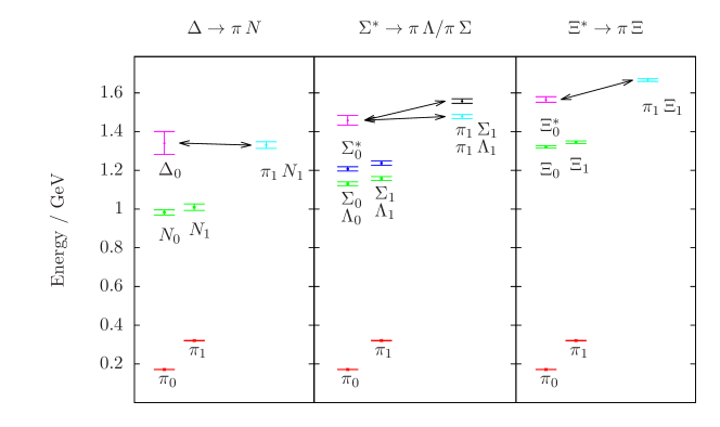
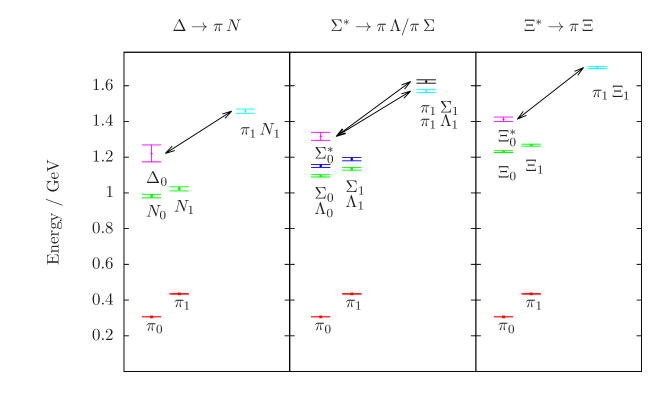
For the unitary ensemble we observe a near degeneracy of energy levels for the $\Delta$ and the $\pi\,N$ scattering state as well as for the $\Sigma^{*}$ and the $\pi\,\Lambda$ scattering state. On the other hand, a significant energy gap exists between the $\Sigma^{*}$ and the $\pi\,\Sigma$ scattering state, and the $\Xi^{*}$ and the $\pi\,\Xi$ scattering state. The situation is qualitatively different for the hybrid calculation, for which the relevant spectrum is shown in Fig. [4]. We observe a larger energy gap for all transitions under consideration, which is roughly the same in all cases.

This qualitative difference arises from the larger values of $m_{\pi}$. In our approximation $E_{MB}=E_{M}+E_{B}$, so the gap is $\delta=E_{B^{*}}-E_{MB}=E_{B^{*}}-E_{M}-E_{B}$. Considering Fig. [4] for the case $\Delta-\pi N$ one observes that at $q=0$, $E_{N}+E_{\pi}$ is significantly greater than $E_{\Delta}$ so $\delta$ is negative and far from threshold. Taking into account that $E_{N}+E_{\pi}$ increases with $q$, and so does $|\delta|$, the gap gets even bigger as compared to $|\delta|$ at zero $q$. The same thing happens for $\Sigma^{*}$ and for $\Xi^{*}$. In contrast, in Fig. [3] for the ensemble at $180\,\mathrm{MeV}$ pion mass, we see that the $\Delta$ is unstable and there is a chance $\delta$ will pass through zero at the relevant $q$ for the transition. Indeed we see that $\delta$ is small and slightly positive. Similarly, for $\Sigma^{*}$, $\delta$ is small and slightly negative.

III.2 $\Delta\to\pi N$

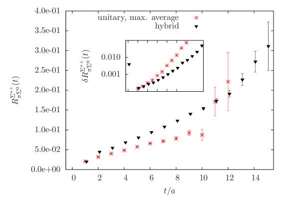
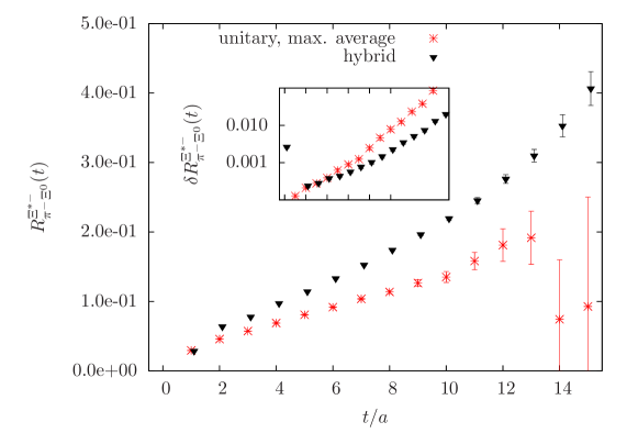
We first discuss the case of the $\Delta$ resonance. As shown in Fig. [3], the lattice kinematics produce a scattering $\pi N$ state that is approximately degenerate with the $\Delta$ mass, thus satisfying one of the conditions for the validity of the method. For the hybrid action, used in our study, the energies have a sizeable gap as shown in Fig. [4]. In Fig. [5] we show the ratio $R^{\Delta}_{\pi\,N}$ for both the unitary and the hybrid action.

Figure 5: Ratio $R^{\Delta}_{\pi N}$ for the unitary and hybrid calculation; the detail plot shows the evolution of the statistical uncertainty with $t/a$. The errors are computed using the $\Gamma$-method Wolff:2003sm . The red crosses are obtained using maximal averaging to construct the ratio for the unitary action, while the blue triangles exploit maximal correlation. The black triangles show the ratio obtained with the hybrid action using maximal correlation combination of data. Data points for different curves have been displaced horizontally.

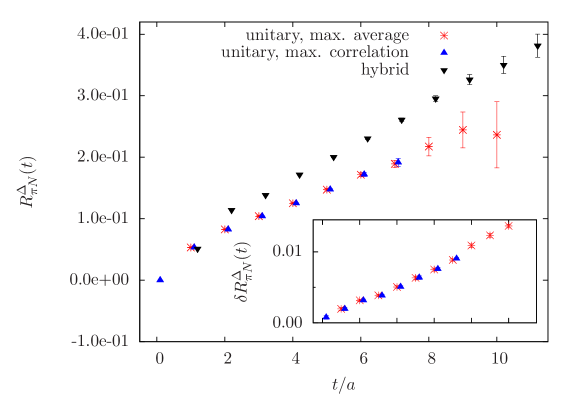
For the unitary case we compare two different ways to combine the available lattice data. In the first one, all individual factors of the two-point correlators entering the ratio are averaged before the ratio is built using the maximal set of lattice symmetries for the individual correlators. This way of combining data will benefit from possible cancellation of additive lattice artifacts in individual correlation functions. We refer to it as maximal averaging. In the second approach, we build the ratio for each data set given by the tuple (momentum / direction, forward and backward propagators, source location) and in the final step combine the individual estimates for the ratio. Since the correlator data within one and the same tuple is maximally correlated, such an average would benefit error cancellations due to statistical correlation.

We note, that due to the coherent source method used with the unitary action, we must keep the source-sink time separation sufficiently smaller than the distance between the source insertions, i.e. $t_{f}-t_{i}\ll T/4$. The ratio $R^{\Delta}_{\pi N}$ shown in Fig. [5] exhibits a time dependence that is consistent with the expected linear behavior for both hybrid and unitary action, as well as for both types of averages. An overall comparison of the two approaches used for constructing the ratio with the unitary action does not reveal any significant difference in the mean value or the statistical uncertainty of the data points where they are both defined. However, on closer examination, the maximally averaged approach produces data for larger time slices. This is due to the fact that the $\Delta$ and nucleon correlators are more accurately determined having thus a lower probability of becoming non-positive in the sampling part of the error estimate. We shall thus use maximal averaging to combine data in what follows.

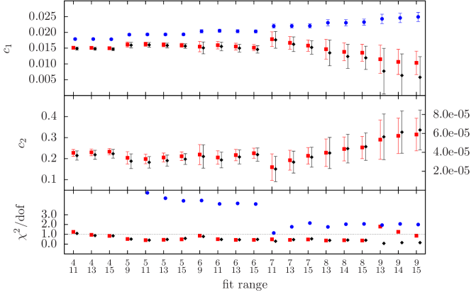
In Fig. [6] we show the results from fitting $R^{\Delta}_{\pi\,N}$ using the two fit ansätze given in Eqs. (21),(22), for the unitary action. We observe that the linear fit ansatz labeled as type 2, which uses a correlated fit with the function $f_{2}(t)$ and two free parameters $c_{0},\,c_{1}$, already leads to fits with a value for $\chi^{2}/\mathrm{dof}$ below one (bottom panel). The fit value for the slope determined by $c_{1}$ does not show significant variation when scanning the fit ranges from $\left[2,\,5\right]$ to $\left[6,\,9\right]$. As shown in Fig. [5], the statistical uncertainty of the fit parameters increases with increasing the lower fit range to larger values as expected from the dependence of the statistical uncertainty on the fitted data. Moreover, using as a fit function $f_{1}(t)$ we do not observe a significant change for $c_{1}$. Neither do we observe any significant dependence of the central value of $c_{1}$ on the number of parameters. In fact, $c_{2}$ is statistically consistent with zero for both ansätze $f_{1}$ and $f_{2}$ as shown in the center panel of Fig. [6]. We point out that we include different labels on the left and right $y$-axes to show the values extracted using the fitting functions $f_{1}$ and $f_{2}$, respectively, because the order of magnitude of $c_{2}$ differs.

Figure 6: We show the values of the parameters $c_{1}$ (upper panel), $c_{2}$ (central panel) and $\chi^{2}/\mathrm{dof}$ for the fit (lower panel) using three different ansätze to fit $R^{\Delta}_{\pi\,N}$. The symbols represent from left to right: type 1 fits using $f_{1}(t)$ with 3 fit parameters (red squares), type 2 using $f_{2}(t)$ with 2 fit parameters (blue circles) and type 3 using $f_{2}$ with 3 fit parameters (black diamonds). The x-label gives the fit interval as a column $t_{\mathrm{min}}$ atop $t_{\mathrm{max}}$ in lattice units; in the case of $c_{2}$ we show results using type 1 with the labels to the left $y$-axis and type 2 with respect to right $y$-axis.

As indicated in Fig. [6], we perform a large number of fits with different fit types using the fit ansätze $f_{1,2}(t)$ and different time ranges for the estimate of the slope and the energies, for zero and one unit of momentum that enter the calculation. We note that with the $\Delta$ at rest, its mass does not enter the calculation of the coupling constant or the width. This result relies on energy conservation and generalizes to all decays studied here.

Since many fits yield an acceptable value for $\chi^{2}/\mathrm{dof}$, we combine the different analyses with an appropriate weight to extract a mean value and meaningful estimates for the statistical and systematic uncertainty to account for the varying goodness of the fits and precision of the estimates from them. We consider the distribution of the results from each individual fit and associate a weight to it as follows:

$$w(g,\,\Gamma) =\prod\limits_{A}\,w(A)$$

$$w(A) =\left(1-2\,|0.5-p_{A}|\right)^{2}\times\mathrm{var}({A})^{-1}\,.$$ (35)

Here, $p_{A}$ denotes the p-value for the fit of quantity $A$,

$$p_{A} =\int\limits_{\chi^{2}_{A}}^{\infty}\,f_{\chi^{2},\,\mathrm{dof}}(X)\,dX\,,$$

where $\chi^{2}_{A}$ is the observed value of $\chi^{2}$ for the fit of quantity $A$ and $f_{\chi^{2},\,\mathrm{dof}}$ the density function for the $\chi^{2}$ distribution for dof degrees of freedom. $A$ runs over all the quantities that have been derived from a fit and enter the calculation of $g$ (or $\Gamma$), i.e. the slope parameter $c_{1}$, the meson mass $m_{M}$ and baryon masses $m_{B}$. The definition in Eq. (35) gives a higher weight to fits with a p-value close to 0.5, such that there is equal probability of finding results above and below the observed fit value, and to those fits with smaller variance of the fit result. We then take a weighted average from the distribution as the mean value,

$$\bar{g} =\sum\limits_{i}\,g_{i}\,w(g_{i})\times\left(\sum\limits_{i}\,w(g_{i})\right)^{-1}\,,$$

where the sum runs over all fits labeled by index $i$. The statistical uncertainty is calculated from the variance of the bootstrap samples for the weighted mean,

$$\delta\,g_{\mathrm{stat}} =\sqrt{\mathrm{var}\left(\bar{g}\right)}\,.$$

Finally, the systematic uncertainty is estimated from the variance of the weighted distribution of the set $\{g_{i}\}$: we form a histogram, where each $g_{i}$ gives a count proportional to $w(g_{i})$ to the corresponding bin. The square root of the variance derived from this distribution gives the systematic error $\delta\,g_{\mathrm{sys}}$. We then quote our results as

$$g =\bar{g}\,\left(\delta\,g_{\mathrm{stat}}\right)\,\left(\delta\,g_{\mathrm{sys}}\right)\,.$$

We proceed in the same way for the evaluation of the width $\Gamma$. Following this procedure, we arrive at the values given in Eqs. (36) and (37).

$$g^{\Delta}_{\pi N}\left(\mathrm{unitary}\right) =23.7\,(0.7)\,(1.1)$$ (36)

$$a\Gamma^{\Delta}_{\pi N}\left(\mathrm{unitary}\right) =0.0868\,(57)\,(32)$$ (37)

III.3 $\Sigma^{*}\to\pi\Lambda$

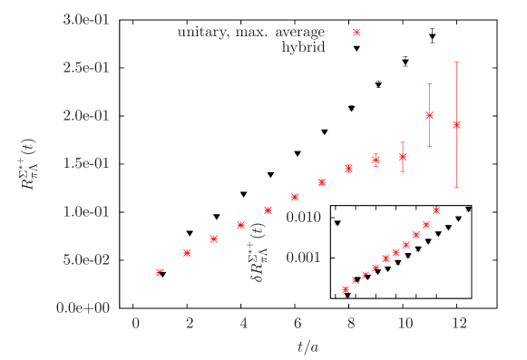
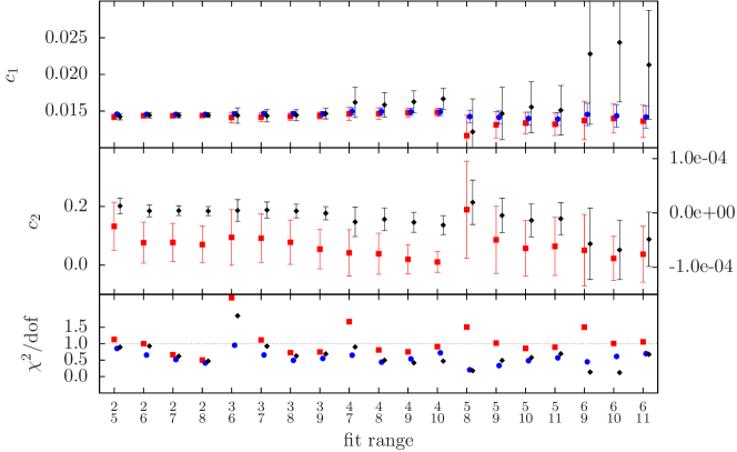
For the decay of the $\Sigma^{*}$, we follow the same approach as in the case of the $\Delta$ decay. In Fig. [7] we show the ratio $R^{\Sigma^{*+}}_{\pi\Lambda}$ for both the unitary and hybrid cases and Figs. [8] and [9] display the behavior of the three different fits when varying the fit ranges. For the unitary action, the energy levels for $\Sigma^{*}$ and $\pi\,\Lambda$ are still close and we find acceptable linear fits already starting at $t_{\mathrm{min}}/a=2$. For the hybrid case we find, that starting with $t_{\mathrm{min}}/a=7$ we find a time independent value for the slope even for the linear fit. The estimates for the slope from the cubic and hyperbolic sine fit are mutually consistent even before that. However, the $\chi^{2}/\mathrm{dof}$ for all fit versions is acceptable starting as early as $t_{\mathrm{min}}/a=5$. A qualitative difference between the unitary and the hybrid ensembles becomes apparent when examining the ratio $R^{\Sigma^{*+}}_{\pi\Lambda}$. When attempting a linear fit to extract the slope, with the hybrid action, the central value for $c_{1}$ rises systematically, when the lower end of the fit window is moved towards larger time-slices. This would be expected for a significant energy gap between the state excited by the $\Sigma^{*}$ and the $\pi\,\Sigma$ interpolating fields. The upward curvature then shows that $E_{\pi\,\Lambda}>E_{\Sigma^{*}}$.

Figure 7: Ratio $R^{\Sigma^{*+}}_{\pi^{+}\Lambda}$ for the unitary and hybrid calculations. The notation is the same as that in Fig. 5.

Figure 8: Fit range dependence of the fit parameters $c_{1},\,c_{2}$ for three different fits of ratio $R^{\Sigma^{*+}}_{\pi^{+}\Lambda}$ for the unitary action. The notation is the same as that of Fig. 6.

Figure 9: Same as Fig. [8], but for the hybrid action.

III.4 $\Sigma^{*}\to\pi\,\Sigma$

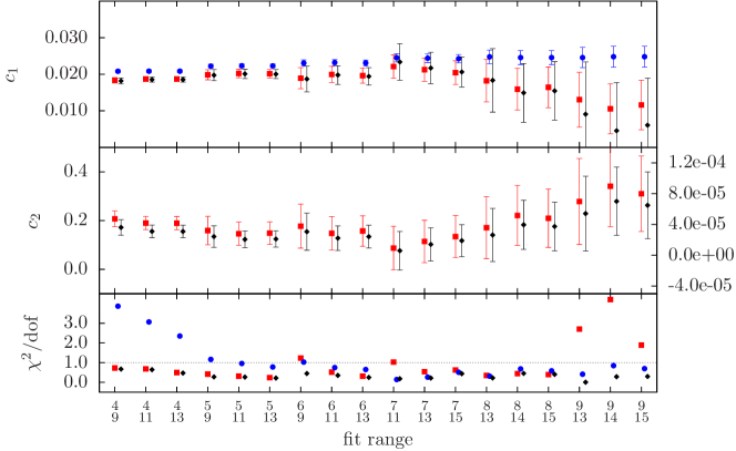
For the transition $\Sigma^{*}\to\pi\,\Sigma$ we show the results for the ratio $R^{\Sigma^{*}}_{\pi\,\Sigma}$ in Fig. [10] and the results for the parameters $c_{1}$ and $c_{2}$ from a variety of our fits in Figs. [11] for the unitary and [12] for the hybrid calculation.

Figure 10: Ratio $R^{\Sigma^{*+}}_{\pi^{+}\Sigma^{0}}$ for the unitary and hybrid calculations.The notation is the same at that in Fig. 5.

Figure 11: Fit range dependence of $c_{1},\,c_{2}$ for three different fits of ratio $R^{\Sigma^{*+}}_{\pi^{+}\Sigma^{0}}$ for the unitary action. The notation is the same as that in Fig. 6.

Figure 12: Same as Fig. [11], but for the hybrid action.

III.5 $\Xi^{*}\to\pi\Xi$

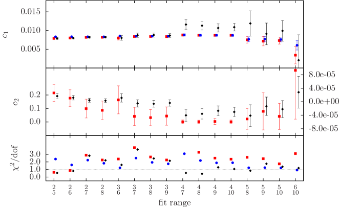
Finally we present the results for the transition $\Xi^{*}\to\pi\,\Xi$ in an analogous manner in Figs. [13], [14] and [15].

Figure 13: Ratio $R^{\Xi^{*-}}_{\pi^{-}\Xi^{0}}$ for the unitary and hybrid calculations.The notation is the same as that in the Fig. 5.

Figure 14: Fit range dependence of $c_{1}$ and $c_{2}$ from the fits of ratio $R^{\Xi^{*-}}_{\pi^{-}\Xi^{0}}$ for the unitary calculation. The notation is the same as that in the Fig. 6.

Figure 15: Same as Fig. [14], but for the hybrid calculation.

We gather our results for the coupling and widths in Tables {5} and {6} below. To allow for an easy comparison we convert the decay widths to physical units using the values for the lattice spacing given in Table {2}.

The results for the process $\Delta\leftrightarrow\pi\,N$ with the hybrid action differ slightly from our previous investigation Alexandrou:2013ata ; Alexandrou:2014qka , since we updated them using the weighted average for the distribution of fits.

Utilizing the expressions of Eqs. (29) and (30) we estimate the coupling, which is independent of the isospin combination of in and out state, while the width is for specific combinations of in and out states. For this reason, in the table we distinguish explicitly the isospin dependence of the width by giving the electromagnetic charges of the interpolating fields as superscripts.

III.6 Improved precision with AMA for $R^{\Delta}_{\pi\,N}$

In order to assess the potential of using all-mode-averaging to improve the accuracy of our computations, we apply all-mode-averaging Blum:2012uh on a subset of 89 (out of 254) configurations and specifically look at the case of $\Delta\to\pi\,N$. In addition to the correlation functions, which had been obtained at high solver precision during the production of quark propagators, a corresponding data set at low solver precision was produced with 16 random shifts of the original spatial source position two-point correlation functions $C_{\Delta-\Delta}$, $C_{\pi-\pi}$ and $C_{N-N}$ for each of the four preset source time-slices independently. The measurements for $C_{\Delta-\pi N}$ are done coherently with a single inversion after inserting sequential sources at the four time-slices.

Figure 16: Comparison of results on the ratio $R^{\Delta}_{\pi\,N}$ with (red squares) and without using all-mode-averaging (blue circles and magenta triangles).

Figure 17: Comparison of the statistical uncertainties of $R^{\Delta}_{\pi\,N}$ with and without using all-mode-averaging; the detail plot shows the ratio of the uncertainty obtained by using AMA over the that from the original run with 254 configurations and 4 source time-slices per configuration; the horizontal line marks the ratio of uncertainties expected for ideal error scaling.

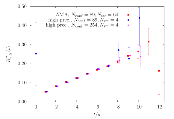
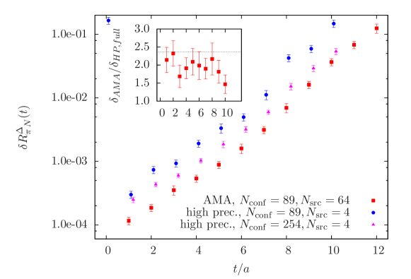
We show a comparison of the estimates for the ratio $R^{\Delta}_{\pi\,N}$ and its statistical uncertainty in Figs. [17] and [17]. We find full consistency of the data for the ratio from both the AMA simulation and the original production run. Moreover, the uncertainty is reduced by a factor around two across the relevant time-slices $1\leq t/a\leq 10$. From an ideal scaling of the error we expect reduction of the statistical uncertainty by a factor of $\sqrt{\left(89\times 64\right)/\left(254\times 4\right)}\approx 2.4$ and the observed behavior is consistent with this expectation.

We determine the coupling and width based on the AMA data set in the way previously outlined and give the results for comparison in Table 3.

	$g^{\Delta}_{\pi\,N}$	$a\Gamma^{\Delta}_{\pi\,N}$
AMA	$24.2\,(0.3)\,(1.0)$	$0.0846\,(23)\,(22)$
HP, full	$23.7\,(0.7)\,(1.1)$	$0.0868\,(57)\,(45)$

Table 3: The results on the $\Delta-\pi N$ coupling constant and width using AMA are shown in the first row, while results extracted without AMA are included in the second row.

The statistical errors show the expected improvement by a factor of approximately 2.4.

IV Discussion

In order to make a direct comparison with the experimental values, we provide in Table 4 the data taken from the Particle Data Group Beringer:1900zz for the relevant baryon and meson masses, the full widths, branching ratios and relative momentum $k$ of the asymptotic final meson and baryon state from the decay in the center-of-mass frame. The coupling constant is then derived according to the tree-level decay process using the expression in Eq. (33) and the experimental value of the width as an input.

We compare these values for the coupling constants to the results of our calculation in Table {5}. The analogous comparison for the decay widths in physical units is shown in Table {6}. We would like to stress that although we show the results for the hybrid and unitary calculation side-by-side in the tables, one should be careful in drawing strong conlcusions since the conditions for the applicability of the transfer matrix method are fulfilled to different degree in the two cases. In particular, the energy matching is very different in the two cases and for a direct comparison one would need to have kinematics where the energy gap is similar.

$B^{*}$	$MB$	$m_{B^{*}}/\,\mathrm{MeV}$	$m_{M}/\,\mathrm{MeV}$	$m_{B}/\,\mathrm{MeV}$	$\Gamma_{\mathrm{full}}/\,\mathrm{MeV}$	$\Gamma^{B^{*}}_{MB}/\Gamma_{\mathrm{full}}$	$p/\,\mathrm{MeV}$
$\Delta$	$\pi\,N$	$1232\,(1)$	$139.57018\,(35)$	$938.272013\,(23)$	$118\,(2)$	$1.$	$227$
$\Sigma^{*}$	$\pi\,\Lambda$	$1382.80\,(35)$		$1115.683\,(6)$	$36.0\,(7)$	$0.870\,(15)$	$205$
$\Sigma^{*}$	$\pi\,\Sigma$			$1192.642\,(24)$		$0.117\,(15)$	$120$
$\Xi^{*}$	$\pi\,\Xi$	$1535.0\,(6)$		$1314.86\,(20)$	$9.9\,(1.9)$	$1.$	$158$

Table 4: The physical values of masses $m_{B^{*}}$, $m_{B}$ and $m_{M}$, full widths $\Gamma_{\mathrm{full}}$, branching ratios $\Gamma^{B^{*}}_{MB}$ and relative momentum $p$ for the 2-hadron state for the resonances studied in this work as given by the Particle Data Group Beringer:1900zz .

process	unitary	hybrid	PDG
$\Delta^{++}\leftrightarrow\pi^{+}\,N^{+}$	$23.7\,(0.7)\,(1.1)$	$26.7\,(0.6)\,(1.4)$	$29.4\,(0.3)$
$\Sigma^{*+}\leftrightarrow\pi^{+}\,\Lambda$	$18.5\,(0.3)\,(0.5)$	$23.2\,(0.6)\,(0.8)$	$20.4\,(0.3)$
$\Sigma^{*+}\leftrightarrow\pi^{+}\,\Sigma^{0}$	$16.1\,(0.3)\,(1.9)$	$19.0\,(0.7)\,(2.9)$	$17.3\,(1.1)$
$\Xi^{*-}\leftrightarrow\pi^{-}\,\Xi^{0}$	$21.0\,(0.3)\,(0.3)$	$25.6\,(0.6)\,(4.3)$	$19.4\,(1.9)$

Table 5: Results for the couplings $g^{B^{*}}_{MB}$. For each decay process given in the first column, we give the coupling constant $g_{MB}^{B^{*}}$ for the unitary DWF ensemble with $m_{\pi}$ = 180 MeV (second column) and hybrid ensemble with $m_{\pi}$ = 350 MeV (third column). The fourth column shows the value of the coupling at leading order effective field theory using input from the PDG. The uncertainties in brackets are statistical and systematic as given in subsection III.2.

process	unitary	hybrid	PDG
$\Delta^{++}\leftrightarrow\pi^{+}\,N^{+}$	$119.4\,(7.9)\,(4.5)$	$238.5\,(12.2)\,(16.2)$	$118\,(2)$
$\Sigma^{*+}\leftrightarrow\pi^{+}\,\Lambda$	$54.5\,(2.1)\,(1.3)$	$143.9\,(7.4)\,(6.1)$	$31.3\,(8)$
$\Sigma^{*+}\leftrightarrow\pi^{+}\,\Sigma^{0}$	$17.6\,(0.8)\,(2.1)$	$58.3\,(3.4)\,(6.8)$	$4.2\,(5)$
$\Xi^{*-}\leftrightarrow\pi^{-}\,\Xi^{0}$	$35.1\,(1.1)\,(0.4)$	$126.0\,(5.6)\,(18.5)$	$9.9\,(1.9)$

Table 6: Results for the decay widths in MeV. The meaning of the columns is analogous to Table {5} with the decay process (first column), results from the unitary DWF ensemble with $m_{\pi}$ = 180 MeV (second column), results from the hybrid ensemble with $m_{\pi}$ = 350 MeV (third column) and the PDG value (fourth column).

We find that our lattice QCD values for the couplings are in good agreement with the PDG-derived values for all decays for both the unitary and the hybrid action with a tendency of higher values for the latter case. This observed level of agreement is remarkable, given that with the unitary and hybrid action we simulate at pion mass $180\,\mathrm{MeV}$ and $350\,\mathrm{MeV}$, respectively, and on coarse lattices.

For the width itself, on the other hand, we only find agreement for $\Gamma^{\Delta}_{\pi\,N}$ with the unitary action. This may be expected since it is only for this case that the energies of the states $B^{*}$ and $M\,B$ are degenerate and therefore this case is the closest to the threshold situation where the conditions of our approach are best fulfilled. Table 4 shows in the right-most column the momentum in the center-of-mass frame for the fields $M$ and $B$ for the individual decays. On the lattice, this momentum is of course fixed to $k=2\pi/L$ in lattice units or $k(\mathrm{unitary})\approx 270\,\mathrm{MeV}$ for the unitary action and $k(\mathrm{hybrid})\approx 357\,\mathrm{MeV}$ for the hybrid one. Thus, in addition to matching the energies of the resonance and the decay channel, one has another constraint, namely, a fixed center-of-mass momentum in these transition processes, which deviates from the physical situation by a process-dependent amount. In general, we have that with the hybrid action, the lattice momentum is 1.5 to 3 times larger than its value in the continuum infinite volume limit. With the unitary action the violation is less severe, and the closest to the physical situation is the one corresponding to decay of the $\Delta$.

Assuming a finite volume we can check that the density of states derived from the lattice values of the masses and the momentum approaches closer to the value of the density of states derived with their continuum counterparts when going from $\pi\,N$ to $\pi\,\Lambda/\pi\,\Sigma$ to $\pi\,\Xi$. This is to be expected, since the strange quark mass is tuned closer to its physical value than the light quark mass and $\Lambda/\Sigma$ and $\Xi$ are have strangeness $-1$ and $-2$, respectively.

The dependence of the coupling and decay width on the meson and baryon masses, momentum and the parameters of the lattice simulation show a large disparity reflected in the different levels of agreement in Tables {5} and {6}. Partly this is explained by the additional condition of having to match the center of mass momentum for extracting the width in the decay process. One would need to study the dependence of the momentum further in order to understand the different level of agreement between the case of the coupling and that of the width.

V Conclusions and Outlook

The coupling constants $g_{\pi N}^{\Delta}$, $g_{\pi\Lambda}^{\Sigma^{*}}$, $g_{\pi\Sigma}^{\Sigma^{*}}$ and $g_{\pi\Xi}^{\Xi^{*}}$ are evaluated using two ensembles of dynamical fermion gauge configurations with pion mass 350 MeV and 180 MeV. In both cases, domain wall valence quarks are used. The gauge configurations for the ensemble with the heavier mass were produced using $N_{f}=2+1$ staggered sea quarks and thus our analysis is done with a hybrid action, while those with the lighter pion mass were produced using $N_{f}=2+1$ domain wall sea quarks so the action is unitary. The kinematical conditions are best satisfied for the unitary action for all four decays, with the $\Delta$-decay being closest to the physical situation. Comparing the values of the coupling constants obtained for these two ensembles, we find that they are about 10% smaller for the ensemble with $180\,\mathrm{MeV}$ pions as compared to their values for the ensemble with 350 MeV pions. Given that the pion mass is about half as compared to the hybrid ensemble, we conclude that the pion mass dependence is rather weak and thus the values obtained using $180\,\mathrm{MeV}$ pions should be close to their values at the physical point, which is indeed what we observe. In order to extract the width, one needs to make further assumptions, some of which are not well satisfied. For example, the energy in the center of mass frame on the lattice is different from the one in the infinite volume limit. The case for which these energies best match is for the $\Delta$-decay where indeed we find an agreement with the experimental value. This demonstrates that the methodology works when the physical kinematical conditions are approximately satisfied on the lattice.

To explore the applicability of AMA on reducing the statistical uncertainty of the ratio and consecutively of the extracted slope, we consider the all-mode-averaging technique for the case of the transition $\Delta\leftrightarrow\pi\,N$. Adding further correlation functions with randomly shifted source positions at low precision for a subset of the gauge ensemble, we increase the available statistics by a factor of approximately $5.6$. The ideally expected reduction of the statistical uncertainty is thus by a factor of $2.4$. We observe an improvement of approximately a factor of $2$ on our final, derived quantities, which is satisfactory. The solver precision for the low-precision inversions of the domain-wall Dirac operator is tuned to a compromise value that, on the one hand, yields sufficiently high statistical correlation for the two-point functions for both high and low precision inversions to ensure a good scaling of the statistical uncertainty with the number of low-precision inversions, and on the other hand, to keep the ratio of cost for a low- to a high-precision propagator as small as possible, which in our case turns out to be 1:5.

Fully exploiting the potential of further reduction of the uncertainty of the slope bears the interesting prospect of becoming sensitive to contributions from excited states and next-to-leading order terms. This would be of particular importance in a more comprehensive, combined analysis of several decay channels and vital for an attempt to tackle the quark-connected diagrams, the calculation of which is beyond the scope of this work. Notwithstanding these future prospects, our current analysis shows, that for the time being, the major source of systematic uncertainty stems from the lattice kinematical setup rather than statistics.

Given the good agreement of our lattice QCD results with the experimental values for the coupling constants and for the width when the kinematical constraints are satisfied, we plan to apply the method to study other baryon decays such as the decay of baryons in the negative parity channel and decays of baryon of higher spin.

In the future we are also planning to address some of the deficiencies of the method connected to the kinematical conditions by considering moving frames. The decays considered here can be the test-bed for these extensions.

References

- (1) M. Luscher, Commun.Math.Phys. 104, 177 (1986).
- (2) M. Luscher, Commun.Math.Phys. 105, 153 (1986).
- (3) K. Rummukainen and S. A. Gottlieb, Nucl.Phys. B450, 397 (1995), hep-lat/9503028.
- (4) Z. Fu, Phys.Rev. D85, 014506 (2012), 1110.0319.
- (5) M. Gockeler et al., Phys.Rev. D86, 094513 (2012), 1206.4141.
- (6) L. Leskovec and S. Prelovsek, Phys.Rev. D85, 114507 (2012), 1202.2145.
- (7) M. Doring, U. Meissner, E. Oset, and A. Rusetsky, Eur.Phys.J. A48, 114 (2012), 1205.4838.
- (8) S. He, X. Feng, and C. Liu, JHEP 0507, 011 (2005), hep-lat/0504019.
- (9) V. Bernard, M. Lage, U.-G. Meissner, and A. Rusetsky, JHEP 0808, 024 (2008), 0806.4495.
- (10) M. Doring and U. G. Meissner, JHEP 1201, 009 (2012), 1111.0616.
- (11) C. Lang, D. Mohler, S. Prelovsek, and M. Vidmar, Phys.Rev. D84, 054503 (2011), 1105.5636.
- (12) R. A. Briceno and Z. Davoudi, Phys.Rev. D88, 094507 (2013), 1204.1110.
- (13) M. T. Hansen and S. R. Sharpe, Phys.Rev. D86, 016007 (2012), 1204.0826.
- (14) P. Guo, J. Dudek, R. Edwards, and A. P. Szczepaniak, Phys.Rev. D88, 014501 (2013), 1211.0929.
- (15) N. Li and C. Liu, Phys.Rev. D87, 014502 (2013), 1209.2201.
- (16) R. A. Briceño, Z. Davoudi, T. Luu, and M. J. Savage, Phys.Rev. D88, 114507 (2013), 1309.3556.
- (17) J.-J. Wu, T.-S. Lee, A. Thomas, and R. Young, Phys.Rev. C90, 055206 (2014), 1402.4868.
- (18) R. A. Briceno and Z. Davoudi, Phys.Rev. D87, 094507 (2013), 1212.3398.
- (19) M. Fukugita, Y. Kuramashi, M. Okawa, H. Mino, and A. Ukawa, Phys.Rev. D52, 3003 (1995), hep-lat/9501024.
- (20) R. A. Briceno, Z. Davoudi, T. C. Luu, and M. J. Savage, Phys.Rev. D89, 074509 (2014), 1311.7686.
- (21) A. Torok et al., Phys.Rev. D81, 074506 (2010), 0907.1913.
- (22) Sinya AOKI for HAL QCD, S. Aoki, Prog.Part.Nucl.Phys. 66, 687 (2011), 1107.1284.
- (23) M. Lage, U.-G. Meissner, and A. Rusetsky, Phys.Lett. B681, 439 (2009), 0905.0069.
- (24) UKQCD Collaboration, C. McNeile, C. Michael, and P. Pennanen, Phys.Rev. D65, 094505 (2002), hep-lat/0201006.
- (25) UKQCD, C. McNeile and C. Michael, Phys.Lett. B556, 177 (2003), hep-lat/0212020.
- (26) C. Michael, Eur.Phys.J. A31, 793 (2007), hep-lat/0609008.
- (27) C. Michael, PoS LAT2005, 008 (2006), hep-lat/0509023.
- (28) C. Alexandrou, J. Negele, M. Petschlies, A. Strelchenko, and A. Tsapalis, Phys.Rev. D88, 031501 (2013), 1305.6081.
- (29) C. Alexandrou, J. W. Negele, and M. Petschlies, PoS LATTICE2013, 281 (2014), 1401.3507.
- (30) V. Pascalutsa and D. R. Phillips, Phys. Rev. C67, 055202 (2003), nucl-th/0212024.
- (31) T. Blum, T. Izubuchi, and E. Shintani, Phys.Rev. D88, 094503 (2013), 1208.4349.
- (32) RBC, UKQCD, R. Arthur et al., Phys.Rev. D87, 094514 (2013), 1208.4412.
- (33) UKQCD Collaboration, C. McNeile, C. Michael, and G. Thompson, Phys.Rev. D70, 054501 (2004).
- (34) Hadron Spectrum, J. J. Dudek, R. G. Edwards, and C. E. Thomas, Phys. Rev. D87, 034505 (2013), 1212.0830, [Erratum: Phys. Rev.D90,no.9,099902(2014)].
- (35) Lattice Hadron Physics Collaboration (LHPC), S. Basak et al., Phys.Rev. D72, 074501 (2005), hep-lat/0508018.
- (36) S. Nozawa and D. Leinweber, Phys.Rev. D42, 3567 (1990).
- (37) C. Alexandrou et al., Phys.Rev. D77, 085012 (2008), 0710.4621.
- (38) C. W. Bernard et al., Phys.Rev. D64, 054506 (2001).
- (39) A. Bazavov et al., Rev.Mod.Phys. 82, 1349 (2010), 0903.3598.
- (40) LHPC, R. Edwards et al., Phys.Rev.Lett. 96, 052001 (2006), hep-lat/0510062.
- (41) A. Walker-Loud et al., Phys.Rev. D79, 054502 (2009).
- (42) C. Alexandrou, T. Korzec, G. Koutsou, J. Negele, and Y. Proestos, Phys.Rev. D82, 034504 (2010), 1006.0558.
- (43) M. Clark, R. Babich, K. Barros, R. Brower, and C. Rebbi, Comput.Phys.Commun. 181, 1517 (2010).
- (44) R. Babich et al., (2011), 1109.2935.
- (45) Qlua software [online], https://usqcd.lns.mit.edu/qlua.
- (46) H. Yin and R. D. Mawhinney, PoS LATTICE2011, 051 (2011), 1111.5059.
- (47) ALPHA collaboration, U. Wolff, Comput.Phys.Commun. 156, 143 (2004), hep-lat/0306017.
- (48) Particle Data Group, J. Beringer et al., Phys.Rev. D86, 010001 (2012).
- (49) A. Strelchenko, M. Petschlies, and G. Koutsou, PRACE Whitepaper (2012).