Anticipating regime shifts in gene expression: The case of an autoactivating positive feedback loop

Abstract

Considerable evidence suggests that anticipating sudden shifts from one state to another in bistable dynamical systems is a challenging task, examples include ecosystems, financial markets, complex diseases, etc. In this paper, we investigate the effects of additive, multiplicative and cross correlated stochastic perturbations on determining regime shifts in a bistable gene regulatory system, which gives rise to two distinct states of low and high concentrations of protein. We obtain the stationary probability density and mean first passage time of the system. We show that increasing additive(multiplicative) noise intensity induces regime shift from a low(high) to a high(low) protein concentration state. However, an increase in cross correlation intensity always induces regime shifts from high to low protein concentration state. For both bifurcation (often called tipping point) and noise induced (called stochastic switching) regime shifts, we further explore the robustness of recently developed critical slowing down based early warning signal (EWS) indicators (e.g., rising variance and lag-1 autocorrelation) on our simulated time series data. We identify that using EWS indicators, prediction of an impending bifurcation induced regime shift is relatively easier than that of a noise induced regime shift in the considered system. Moreover, the success of EWS indicators also strongly depends upon the nature of noise. Our results establish the key fact that finding more robust indicator to forewarn regime shifts for a broader class complex natural systems is still in its infancy and demands extensive research.

I Introduction

Theoretical as well as experimental studies have indicated that many complex systems under the influence of stochastic perturbations can undergo sudden “regime shifts” in which they abruptly shift to a contrasting state. Such shifts may occur in systems with alternative stable states Sc01 . Well studied examples of regime shifts include sudden collapse of ecosystems RiRuKo04 , the onset of collapse in mutualistic communities DaBa14 , abrupt climatic shifts LeHeKr08 , the crash of markets in global finance MaLeSu08 , systemic failures such as the epileptic seizures Mc03 and even the eruptive events in spreading fires FoWh15 . Despite rich advances in the theory of complex systems, understanding the mechanism which trigger the onset of regime shifts in nature remains a challenge.

There are mainly two types of regime shifts that can occur in systems with alternative stable states. One is critical transition which is associated with the bifurcation points (so called tipping points) Scheffer:2012sc and another is noise induced transition (also known as stochastic switching) Boettiger:2013jc . Much effort has been devoted in recent years in developing early warning signals of impending regime shifts between alternative stable states (CaBr06, ; CaBr08, ; GuJa08, ; ScJo09, ; Se11, ; Dakos:2012pone, ; Kefi:2014pone, ). Such early warning signals can have tremendous impact on managing natural systems by forewarning the systems under the threat of state shift, so that appropriate management strategies can be initiated to prevent a catastrophe. Recent progress in this direction suggests that a set of generic statistical indicators (e.g., increase in variance, autocorrelation) may forewarn an impending transition in a wide range of complex systems (ScJo09, ). A recent review on “dynamical disease” argued that an early detection of regime shifts even in the field of medical sciences, such as in cardiac arrhythmia’s could be of some help to prevent sudden death gl15 . However, these signals are mostly developed for the phenomenon of critical slowing down that arises in the vicinity of tipping points (ScJo09, ; DaCa15, ). For purely noise induced transitions, such as we also examine in this paper, there is an active debate about whether early warning signals can really be useful (Drake:2013cb, ; Boettiger:2013jc, ; DaCa15, ).

In genetic regulatory systems, it is known that random cell-to-cell variations within a genetically identical population can lead to regime shifts between alternative stable states of gene expression (i.e., sudden transition in protein concentration) (KaEl05, ; MaRaDu07, ). When the underlying genetic system contains regulatory positive feedback loops, individual cells can exist in different steady states (AnFeSo04, ). Some cells may, for example, live in the “off” expression state of a particular gene, whereas others are in the “on” expression state (ThPoGr14, ). These stochastic fluctuations in gene expression, commonly referred to as noise, have been proposed to cause transitions between these states (Oz04, ; AcBeOu05, ). A well known example of bistable gene expression with coupled stochastic transition is the induction of the lac operon in E. coli which results in the synthesis of protein $\beta$-galactosidase required for breaking up sugar molecules and releasing energy to the cell Muhi . Experimental study on $\beta$-galactosidase shows that sudden transition from unregulated (low level) to regulated (high level) $\beta$-galactosidase state of lac operon occurs at a critical point of an inducer concentration Oz04 . A potential application of early warning signals in gene expression is to identify increased risk of sudden transitions in protein concentration and prevent complex disease onset gl15 ; TrAn15 ; ChLi12 .

Recently the concept of regime shifts with associated early warning signals has been used in systems medicine TrAn15 . The expectation is to foresee a sudden catastrophic shift in health condition which may result in a extreme transition to a disease state. Now a days it is believed that a detailed understanding of regime shifts in disease onset will provide broad applications in the field of medicine TrAn15 . Already detected sudden transitions in medical science include epileptic seizures McSmTa:2003NatMed , depression Leemput07012014 , pulmonary disease Venegas:2005Nat , diabetes mellitus LiLiZh2013 , etc. For the case of type 1 diabetes mellitus, $\beta$-cells in the pancreas do not produce protein hormone insulin, which sometimes is a consequence of “switched off” state of HLA-encoding genes in the cell (“switched on” state of genes in $\beta$-cell corresponds to activation of insulin production). This is due to the fact that genes carry the instructions that cells use for protein production. Hence, bistability via “switching on” or “off” states in “gene expression” is also an important topic to study for regime shifts in systems medicine TrAn15 .

In this paper, we study a stochastic version of bistable gene regulatory positive feedback loop model Ch08 to explore the robustness of early warning indicators of regime shifts, for both cases, the critical transition and noise induced transition. We investigate the effect of additive and multiplicative noise intensities, and cross correlation intensity between two noises on the model by calculating the probability density and potential function.We find that increasing the intensity of additive noise induces regime shifts from low to high protein concentration state and vice versa for an increase in multiplicative noise intensity. Whereas an increase in the cross correlation intensity from a negative to a positive value between the two noises induce regime shifts from high to low protein concentration state. We also compute mean first passage time (MFPT) for escape over the potential barrier. We discuss how one can regulate the production levels of protein. To this end, we apply the early warning signals of regime shifts (ScJo09, ) on the simulated time series data of the stochastic model to examine how successfully one can forewarn regime shifts. Our work presents a novel framework for using early warning signals to identify regime shifts, and also their key limitations, in a gene regulatory system. Finally, in the discussion section, we conclude the paper with a discussion of the main results together with the applicability and importance of our study.

II A model of genetic regulation

II.1 Deterministic description

It is well known that autoactivating positive feedback loop is one of the simplest circuit motifs able to exhibit bistable states in gene regulatory process BeSeSe01 ; TyChNo03 ; LiJi04 ; Ch08 ; Frcasaib12 . In the circuit, a single gene encodes a transcriptional factor activator (TF-A), and the TF-A activates its own transcription when bind to a responsive element (TF-RE) in the DNA sequence (see Fig. 1 for a schematic representation). The transcription factor activator TF-A is referred to as regulatory protein, is used to control genetic regulation and acts as a pathway mediating a cellular response to a stimulus. The TF-A constructs a homodimer which then binds to TF-RE or DNA regulatory site. Gene incorporates a TF-RE and when homodimers bind to the TF-RE, transcription of TF-A is increased. Homodimer binding to responsive element is independent phosphorylation of dimers. However, transcription can be activated only by phosphorylated TF-A dimers. Some dimers phosphorylation will depend on activity of kinases and phosphatases which is controlled by external signals. Hence, this genetic circuit incorporates signal-activated transcription as well as positive feedback on TF-A synthesis. Let, $X$ denotes the protein TF-A, $D$($D^{*}$) denotes the unbound(bound) state of the DNA promoter, then the equilibrium reactions can be written as:

$\displaystyle\varnothing\underset{k_{deg}}{\stackrel{{\scriptstyle RV}}{{\rightleftharpoons}}}X,$

$D+nX$ $\displaystyle\underset{k_{2}}{\stackrel{{\scriptstyle k_{1}/V^{n}}}{{\rightleftharpoons}}}$ $D^{*},$

$D^{*}$ $\displaystyle\overset{k_{p}}{\rightarrow}$ $D^{*}+X,$

where $R$ is the basal expression rate, $V$ is cellular volume, $X$ is degraded with a rate constant $k_{deg}$, $n$ represents cooperativity in binding, binding(unbinding) of TF-A homodimer to DNA regulatory site with a rate constant $k_{1}$ ($k_{2}$) and $k_{p}$ is protein production rate of TF-A. Letting $x=[X]$, $d=[D]$ and $d^{*}=[D^{*}]$, the rate equation of the evolution of concentration of TF-A can be written as WeBu13 :

$$\frac{dx}{dt}=R+a\frac{x^{n}}{K_{d}+x^{n}}-k_{deg}x,$$ (1)

where $a=k_{p}(d+d^{*})$ is the maximum production(i.e., transcription) rate, $K_{d}=k_{2}/k_{1}$ is the dissociation constant of TF-A from TF-RE. A more detail derivation of Eq. (1) is given in WeBu13 .

Figure 1: A schematic picture of genetic expression for an auto-activating positive feedback loop. The expression of gene leads to protein (TF-A) that after oligomerization binds to its own promoter (TF-RE), acting as an self activator. Degradation of the protein is denoted by the slashed circle ($\varnothing$).

We can rewrite the dimensionless version of Eq. (1) as

$$\frac{d\tilde{x}}{d\tilde{t}}=\tilde{r}+\tilde{a}\frac{\tilde{x}^{n}}{1+\tilde{x}^{n}}-\tilde{x},$$ (2)

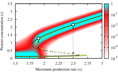
where $\tilde{x}=\frac{x}{\sqrt[n]{K_{d}}}$, $\tilde{t}=k_{deg}t$, $\tilde{a}=\frac{a}{k_{deg}\sqrt[n]{K_{d}}}$, and $\tilde{r}=\frac{R}{k_{deg}\sqrt[n]{K_{d}}}$. The analyses in this work have been carried out using the above model with dimensionless variable and parameters. For certain parameter values, Eq. (2) has three equilibria, of which two are attractors and third is a saddle point intermediate between the two attractors (see Fig. 2). The saddle point works as a basin boundary between the two stable equilibrium points. A thorough analysis of the deterministic model is given in Sm98 . Hereafter, in Eq. (2) for sake of simplicity we use $x$, $t$, $r$ and $a$ in place of $\tilde{x}$, $\tilde{t}$, $\tilde{r}$ and $\tilde{a}$ respectively, and Eq. (2) becomes:

$$\frac{dx}{dt}=r+a\frac{x^{n}}{1+x^{n}}-x\;.$$ (3)

If $n>1$ and $0<r<1/3\sqrt{3}$, then Eq. (3) exhibits bistability for a range of the parameter $a$ WeBu13 . To avoid lengthy calculations, we now replace $n=2$ in Eq. (3), in the rest of this paper.

Figure 2: Bifurcation diagram for the deterministic model (black) and the stochastic model (green). The parameter values are $r=0.1$ (for the deterministic model) and $r=0.1$ with $\sigma_{1}=0.1$, $\sigma_{2}=0.1$ and $\lambda=0.1$ (for the stochastic model). Stable steady states are marked with continuous lines and unstable steady states are marked with dashed lines, respectively. The stationary probability distribution for the additive noise model, Eq. (4 ), for different values of the production rate $a$ is shown in cyan-red-white scale (color bar, logarithmic scale).

To model (3), we investigate the effects of additive and multiplicative noise on the alternative steady states of the gene regulatory circuit. We make this attempt because in the presence of noise, a bistable system may trigger regime shifts.

II.2 Stochastic description

It is well known that noise is inherent in any natural system. In this work, we consider that dynamics of the protein concentration ($x$) are affected by multiplicative and additive noises, similar to Hasty et al. Ha00 . These noise terms can induce sudden shifts in the concentration of protein ($x$). In a bistable system, in the absence of noise the system will eventually converge to one of its two stable fixed points. In which fixed point it will converge depends upon the initial condition. However, the presence of noise in the system will cause fluctuations in the steady states WhoRle84 , which may lead to switching between two different stable states DaCa15 or there can be sudden transition from one stable state to the other stable state DaCa15 . In order to introduce the multiplicative and additive noise terms in Eq. (3), we consider the one-variable Langevin equation in the general form as:

$$\frac{dx}{dt}=f(x)+g(x)\xi(t)+\eta(t),$$ (4)

where $\xi(t)$ and $\eta(t)$ represent Gaussian white noise. These noise terms have the following statistical properties: $\langle\xi(t)\rangle=\langle\eta(t)\rangle=0$, $\langle\xi(t)\xi(t^{\prime})\rangle=2\sigma_{1}\delta(t-t^{\prime})$, $\langle\eta(t)\eta(t^{\prime})\rangle=2\sigma_{2}\delta(t-t^{\prime})$, and $\langle\xi(t)\eta(t^{\prime})\rangle=\langle\eta(t)\xi(t^{\prime})\rangle=2\lambda\sqrt{\sigma_{1}\sigma_{2}}\;\delta(t-t^{\prime})$, where $\sigma_{1}$ and $\sigma_{2}$ measure the level of noise strengths of $\xi(t)$ and $\eta(t)$ respectively, $\lambda$ is the cross correlation between them, and $t$ and $t^{\prime}$ denote two different moments.

(a)

(b)

Figure 3: Example time series datasets exhibiting regime shifts: (a) Critical transition (associated with bifurcation) and (b) Stochastic switching (purely noise induced) for the considered stochastic model. See text for more details.

In Eq. (4) the additive noise $\eta(t)$ alters the background protein production Ha00 . It is also known that in gene expression, transcription is a complex sequence of reactions Leh_book , thus it is expected that this part of the gene regulatory sequence is also to be affected by fluctuations of many intrinsic or extrinsic parameters. This implies the fact that the transcription rate ($a$) can be considered as a random variable Ha00 . To vary the transcription rate stochastically, we consider $a\rightarrow a+\xi(t)$. Hence, with the aforementioned modification, Eq. (3) (for $n=2$) becomes:

$$\frac{dx}{dt} = r+\frac{ax^{2}}{1+x^{2}}-x+\frac{x^{2}}{1+x^{2}}\xi(t)+\eta(t)\;,$$

$$= f(x)+g(x)\xi(t)+\eta(t)\;,$$

where, $f(x)=r+\frac{ax^{2}}{1+x^{2}}-x$ and $g(x)=\frac{x^{2}}{1+x^{2}}$. Hence, the noise $\xi(t)$ is multiplicative, as compared to the additive noise $\eta(t)$.

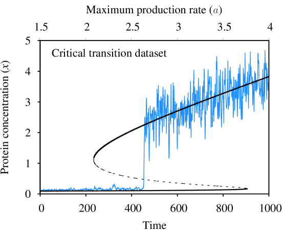
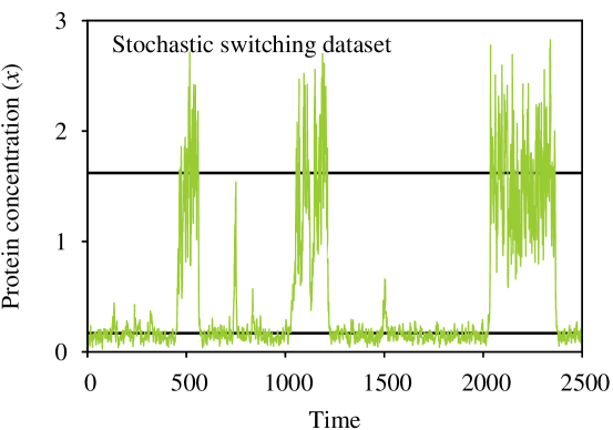
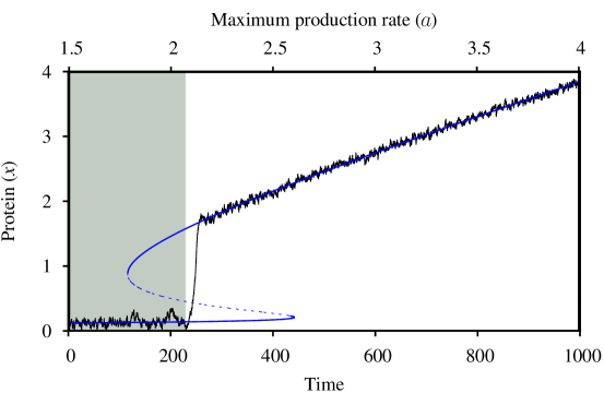
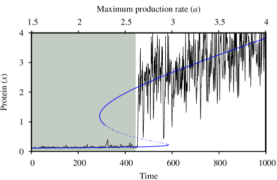
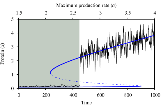
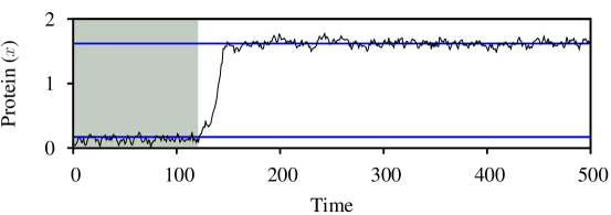
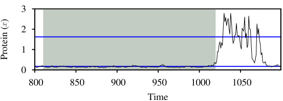
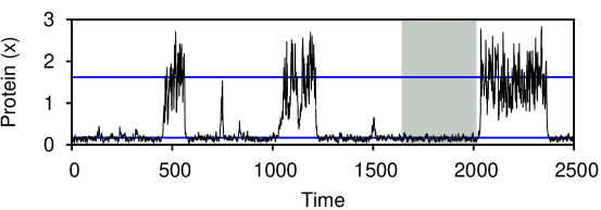
In the next section we study the stochastic model Eq. (II.2) through a combination of analytical and simulation techniques. Our main aim is to investigate the effects of multiplicative noise intensity $\sigma_{1}$, additive noise intensity $\sigma_{2}$ and cross correlation strength $\lambda$ between two noises on the regime shifts between the high and low protein concentration states. In the analytical technique these effects are studied by calculating probability densities, potential functions and MFPT. The simulation technique is complementary to the analytical technique, showing how the dynamical properties are captured in our analytical results can be seen within individual realizations based on example parameter sets, and adding information about how observed protein concentrations are arranged in time in these examples. In simulations, we also produce time series exhibiting regime shifts that can be analyzed using the same techniques as could be applied to real time series data (see Figs. 3(a)-(b)). The example times series can be divided into two broader classes: (a) critical transition time series (Fig. 3(a)) and (b) purely noise induced transition time series (Fig. 3(b)).

III Results

III.1 Fokker-Planck equation and stationary probability density function

We begin this section by writing down the Fokker-Planck equation for the evolution of probability density of the dynamical variable $x$ WhoRle84 . Let $P(x,t)$ denotes the probability density, which is the probability that the protein concentration attains the value $x$ at time $t$. Then, the Fokker-Planck equation (FPE) of $P(x,t)$ corresponding to Eq. (II.2) is given by Ri96 :

$$\frac{\partial P(x,t)}{\partial t}=-\frac{\partial}{\partial x}[A(x)P(x,t)]+\frac{\partial^{2}}{\partial x^{2}}[B(x)P(x,t)]\;,$$ (6)

where

$$A(x) = f(x)+\sigma_{1}g(x)g^{\prime}(x)+\lambda\sqrt{\sigma_{1}\sigma_{2}}\;g^{\prime}(x),\;\text{and}$$

$$B(x) = \sigma_{1}\left[g(x)\right]^{2}+\sigma_{2}+2\lambda\sqrt{\sigma_{1}\sigma_{2}}\;g(x).$$

The limit of $P(x,t)$ as $t\rightarrow\infty$ yields the stationary probability density function (SPDF) of $x$, which we denote as $P_{s}(x)$. The SPDF $P_{s}(x)$, which is the stationary solution of the FPE in Eq. (6) is given by Ri96 (see Appendix S1 for more details) :

$$P_{s}(x) = \frac{N_{c}}{B(x)}\exp\left[\int^{x}\frac{A(x^{\prime})}{B(x^{\prime})}dx^{\prime}\right],$$

$$= \frac{N_{c}}{\sigma_{1}\left[g(x)\right]^{2}+\sigma_{2}+2\lambda\sqrt{\sigma_{1}\sigma_{2}}\;g(x)}\times$$

$$\!\!\!\!\!\!\!\!\!\exp\left[\int^{x}\frac{f(x^{\prime})+\sigma_{1}g(x^{\prime})g^{\prime}(x^{\prime})+\lambda\sqrt{\sigma_{1}\sigma_{2}}\;g^{\prime}(x^{\prime})}{\sigma_{1}\left[g(x^{\prime})\right]^{2}+\sigma_{2}+2\lambda\sqrt{\sigma_{1}\sigma_{2}}\;g(x^{\prime})}dx^{\prime}\right],$$

Figure 4: Potential landscapes demonstrating how changes in a system parameter can cause decrease in resilience of equilibrium point. Recovery rates upon stochastic fluctuations are lower if the basin of attraction is small (d) than that of a larger basin of attraction (a). The effect of reduced resilience can be determined by stochastic fluctuations induced in a system state ((b) and (e)) as increased standard deviation (S.D.) and lag-1 autocorrelation ((c) and (f)). Data sets to plot this figure are generated from Eq. (II.2) with $r=0.1$, $\sigma_{1}=0.0$, $\sigma_{2}=0.05$: (a-c) $a=2.5$ and (d-f) $a=1.9$.

where $N_{c}$ is normalization constant. Equation (LABEL:Eq:SPDF1) can also be put in the form:

$$P_{s}(x)=N_{c}e^{-\phi(x)}\;,$$ (8)

where

$$\phi(x)=\frac{1}{2}\ln\left[\sigma_{1}\left[g(x)\right]^{2}+\sigma_{2}+2\lambda\sqrt{\sigma_{1}\sigma_{2}}\;g(x)\right]$$

$$-\int^{x}\frac{f(x^{\prime})dx^{\prime}}{\sigma_{1}\left[g(x^{\prime})\right]^{2}+\sigma_{2}+2\lambda\sqrt{\sigma_{1}\sigma_{2}}\;g(x^{\prime})}\;,$$ (9)

is called stochastic potential of the system Ri96 . The potential function maps the equilibria of dynamical systems and their basins of attraction, by analogy to a “energy landscape” in which the system state tends to move “downhill”. Extending this concept to stochastic dynamical systems gives a probabilistic potential $\phi(x)$ that complements the SPDF $P_{s}(x)$ in characterizing the asymptotic behavior of the considered system. Next we calculate $\phi(x)$ and $P_{s}(x)$ for three different cases concerning the effects of multiplicative and additive noise on anticipating regime shifts in gene expression. We also calculate bifurcation diagram (see Fig. 2) with changing the maximum transcription rate $a$ for both the deterministic and stochastic model. Note that, there is an enlargement of the bistability region for the case of correlated noise. In Fig. 2, we depict the stationary probability distribution of the additive noise model for different values of $a$, which is shown in white-red-cyan colorbar. This gives an idea about how extrema of stationary probability distribution is changing with the parameter $a$. Now, using analytical techniques we first determine the parameter space where the system persists bistability still in the presence of stochasticity. Then, for a specific set of parameter values, we simulate time series of the system and finally using EWS indicators Scheffer:2012sc , we will try to detect forthcoming regime shifts.

III.1.1 Additive noise

First, we present the effect of an additive external noise source on the regime shifts between high and low concentrations level of protein in gene expression. Hence, only the additive noise term is present in Eq. (II.2) and we assume that $\sigma_{1}=0$. Bifurcation diagram and stationary solutions of the additive noise model are same as for the deterministic model Frcasaib12 . For $\sigma_{1}=0$, the FPE (6) can be written as:

$$\frac{\partial P(x,t)}{\partial t}=-\frac{\partial}{\partial x}[f(x)P(x,t)]+\sigma_{2}\frac{\partial^{2}}{\partial x^{2}}[P(x,t)],$$ (10)

and similar to Eq. (8) the stationary solution $P_{s}(x)$ is written as:

$$P_{s}(x)=N_{A}e^{-\phi(x)}\;,$$ (11)

where

$$\phi(x)=\frac{1}{2}\ln\sigma_{2}-\frac{1}{\sigma_{2}}\int^{x}f(x^{\prime})dx^{\prime}\;,$$ (12)

is the potential and $N_{A}$ is the normalization constant.

Figure 5: (a)–(c) The effect of maximum production rate $a$ on the stochastic potential $\phi(x)$, when only additive noise is present in the system: (a) $a=1.3$, (b) $a=1.9$, and (c) $a=2.7$ with $r=0.1$ and $\sigma_{2}=0.05$. (d)–(f) The effect of additive noise strength $\sigma_{2}$ together with maximum production rate $a$ on the SPDF $P_{s}(x)$: (d) $a=1.3$, (e) $a=1.9$, and (f) $a=2.7$ with $r=0.1$ and for three different noise strengths $\sigma_{2}=0.05$ (black curve) , $\sigma_{2}=0.1$ (red curve) and $\sigma_{2}=0.2$ (blue curve).

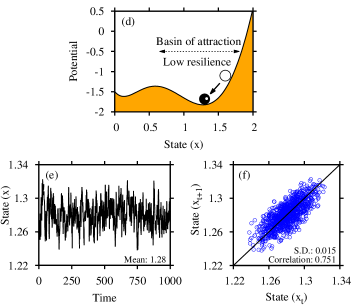
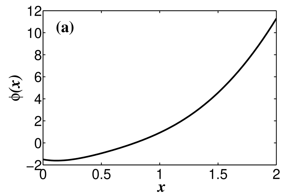
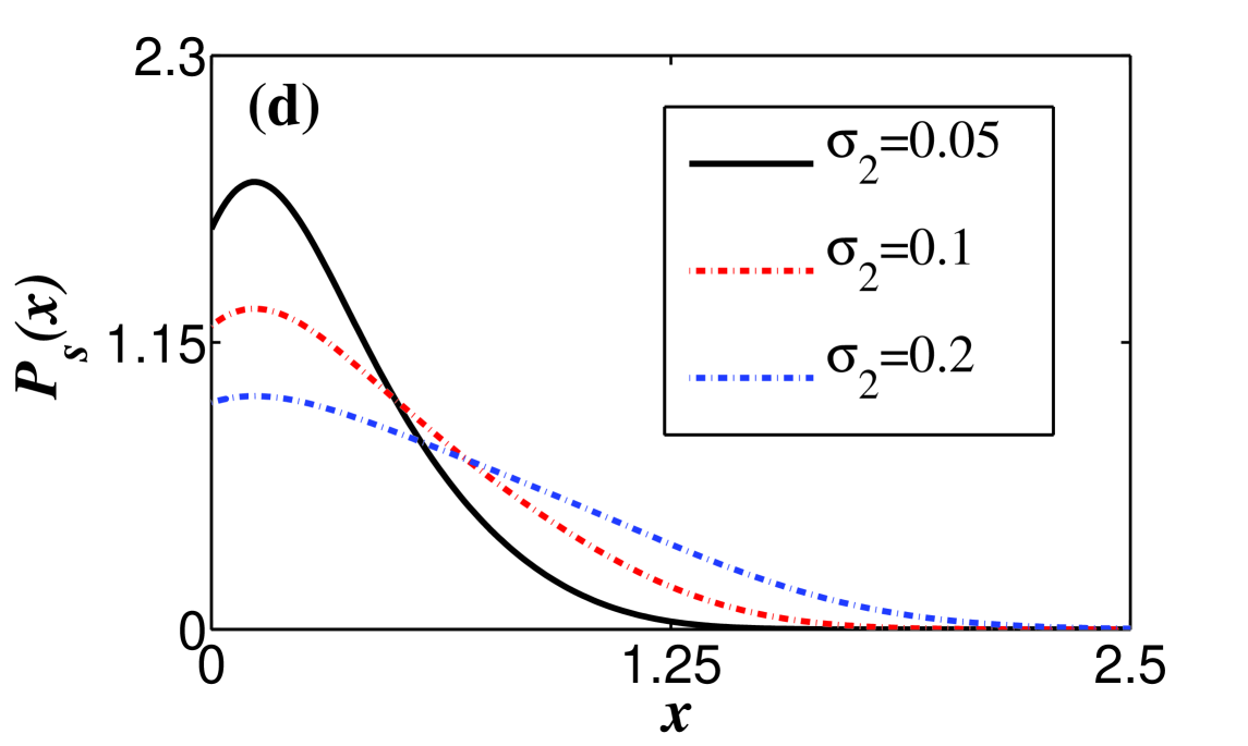
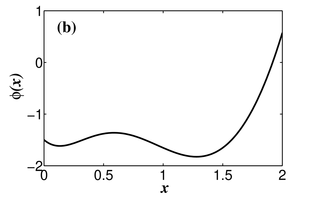
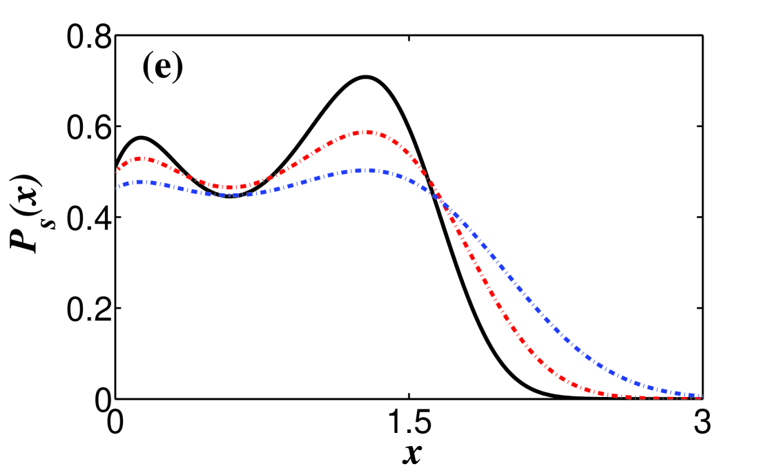
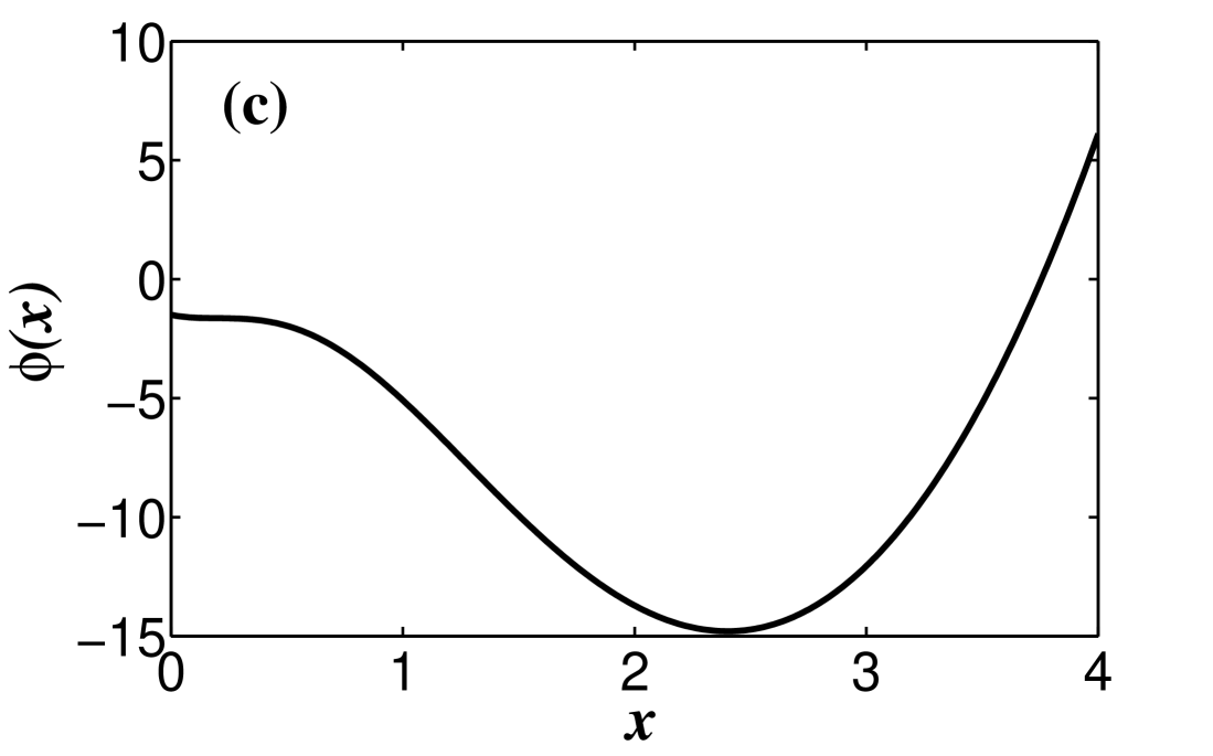
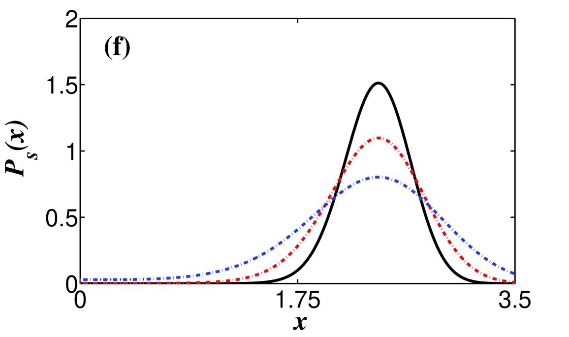
Figures 4(a) and 4(d) show the effective potential at two different values of $a$ with a non-zero additive noise intensity. The depth and width of a potential well can be related to its resilience. Resilience is defined as the ability of a system to recover to its original state upon a perturbation. For critical transitions as the system approaches to a bifurcation point (see the positions of the parameter $a$ in Fig. 2 marked by circles) the recovery rate from perturbation decreases smoothly, known as critical slowing down and as a result the system loses its resilience. One important prediction is that the loss of resilience should lead to an increase in the standard deviation and autocorrelation (see Figs. 4(c) and 4(f)) Scheffer:2012sc . Next, we have demonstrated how the probability distribution of a system can be related with its potential and acts as a mapping between potential and their resilience. We simultaneously try to see the effect of changes in the parameter $a$ and noise intensity on regime shifts.

The effect of changing the maximum production rate $a$ on the stochastic potential $\phi(x)$ and simultaneously changing $a$ together with different additive noise intensity $\sigma_{2}$ on SPDF $P_{s}(x)$ is depicted in Fig. 5. In the left panel of Fig. 5, we show that by varying $a$ from low (see Fig. 5(a)) to high values (see Fig. 5(c)), the system can pass from a monostable low protein concentration state (Fig. 5(a)) through a region of bistability (Fig. 5(b)) (i.e. coexistence of low and high concentration states) to a monostable high concentration state (Fig. 5(c)). For $a=1.9$, the region of bistability is distinguished by the presence of two local minima in the potential $\phi(x)$ (see Fig. 5(b)). As already stated, the depth and width of the potential well determine the resilience of the equilibrium point. It is evident from Fig. 5(b) that the high concentration protein state ($x$) has high resilience. Hence, in a stochastic environment it has a low risk to experience a regime shift and can sustain under large disturbance in comparison with the low concentration protein state. On the other hand in stochastic models, peaks of the SPDF $P_{s}(x)$ correspond to attractors and troughs correspond to repellors. Moreover, an equilibrium point is more stable (high resilience) if the SPDF peak is large in comparison with another equilibrium point which is less stable (low resilience) as the SPDF peak is small. The effect of three different values of noise intensity $\sigma_{2}$ on SPDF $P_{s}(x)$ is shown in Figs. 5(d)–5(f) for three different values of $a$. In case of bistability, for a fixed $a=1.9$, if we slowly increase the noise strength $\sigma_{2}$, the system still has coexistence of low and high concentration protein state for low value of $\sigma_{2}$. As we further increase $\sigma_{2}$, the system will slowly shift to a single state consists of high protein concentration only (see Figs. 5(e)–5(f)). This regime shift is expected as because for $a=1.9$ the high protein concentration state has high resilience.

III.1.2 Multiplicative noise

Next, we consider only the presence of multiplicative noise in the system, i.e., in Eq. (II.2) the strength of additive noise $\sigma_{2}=0$. For $\sigma_{2}=0$, the FPE (6) becomes:

$$\frac{\partial P(x,t)}{\partial t}=-\frac{\partial}{\partial x}\left[A(x)P(x,t)\right]+\frac{\partial^{2}}{\partial x^{2}}\left[B(x)P(x,t)\right],$$ (13)

where

$$A(x) = f(x)+\sigma_{1}g(x)g^{\prime}(x),\;\;\text{and}$$

$$B(x) = \sigma_{1}\left[g(x)\right]^{2}.$$

The stationary solution $P_{s}(x)$ of Eq. (13) is:

$$P_{s}(x)=N_{M}e^{-\phi_{(}x)},$$ (14)

where

$$\phi_{(}x)=\frac{1}{2}\ln\left[\sigma_{1}\left[g(x)\right]^{2}\right]-\int^{x}\frac{f(x^{\prime})dx^{\prime}}{\sigma_{1}\left[g(x^{\prime})\right]^{2}}\;,$$ (15)

is the stochastic potential and $N_{M}$ is the normalization constant.

Figure 6: (a)–(c) The effect of maximum production rate $a$ on the stochastic potential $\phi(x)$, when only multiplicative noise is present in the system: (a) $a=1.2$, (b) $a=2.3$, and (c) $a=3$ with $r=0.1$, $\sigma_{1}=0.65$ and $\sigma_{2}=0$. (d)–(f) The effect of noise strength $\sigma_{1}$ together with maximum production rate $a$ on the SPDF $P_{s}(x)$: (d) $a=1.2$, (e) $a=2.3$, and (f) $a=3$ with $r=0.1$ and for three different noise strengths $\sigma_{1}=0.15$ (black curve), $\sigma_{1}=0.25$ (red curve) and $\sigma_{1}=0.65$ (blue curve).

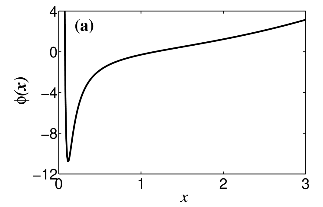
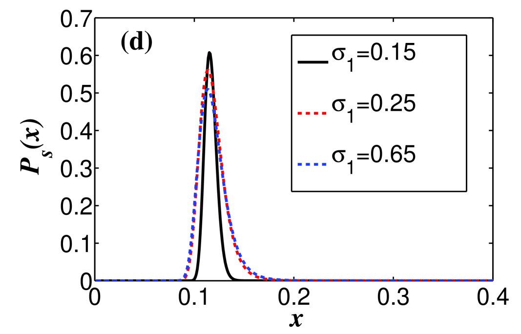
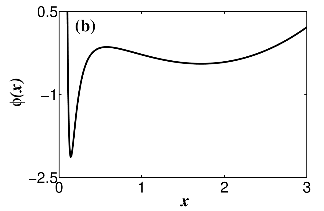
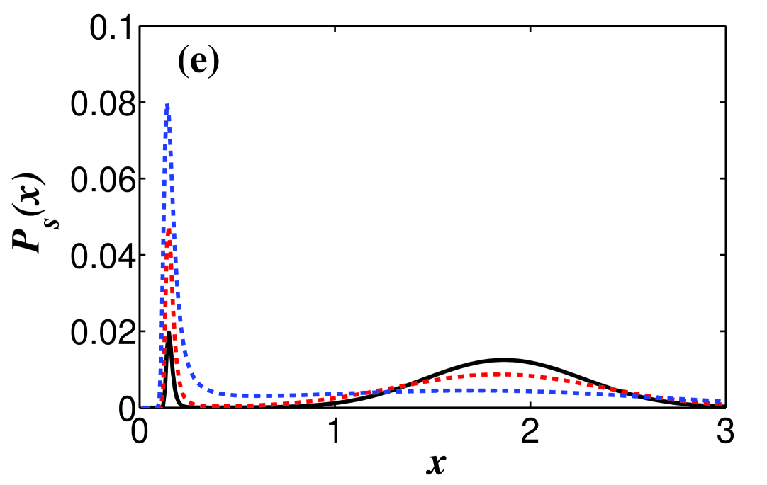
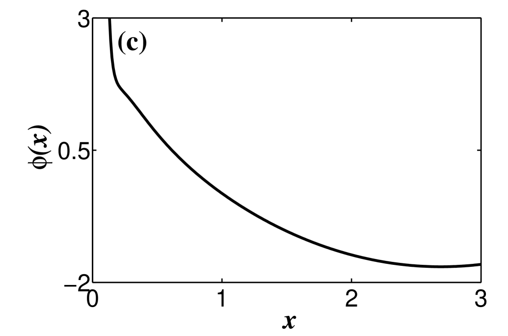
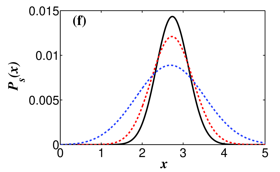
Similar to the case of additive noise in the previous section (Sec. III.1.1), here Fig. 6 shows the effect of changing the parameter $a$ and the noise intensity $\sigma_{1}$ on the potential function $\phi(x)$ and the SPDF $P_{s}(x)$. In one hand, when we increase the parameter $a$ with a fixed noise intensity (see Figs. 6(a)–6(c)), the system passes through a low concentration state to a high concentration state via a bistable region (Fig. 6(b)). On the other hand, with variations in $a$ we plotted the SPDF for different values of the noise intensity $\sigma_{1}$ (see Figs. 6(d)–6(f)). For monostable regions the effect of noise intensity on $P_{s}(x)$ is similar, with an increase in $\sigma_{1}$ the SPDF peak is decreasing. However, in the bistable region (Fig. 6(e)), with an increase in $\sigma_{1}$, the SPDF peak at the low protein concentration $x$ is increasing and that of the high protein concentration $x$ is decreasing. This actually supports the fact that when there is bistability in the system, the low concentration state is more resilient (more stable under perturbative condition) than that of the high concentration state, which is also evident from the Fig. 6(d).

III.1.3 Additive and multiplicative noise with correlation

Herein, we consider that both the additive and multiplicative noise $\eta(t)$ and $\xi(t)$ are present in the system Eq. (II.2). Moreover, both these noise are statistically correlated with a cross correlation parameter $\lambda$. The correlation can arise from the regulation of feedback mechanism, i.e., in the presence of noise the protein concentration $x$ is chemically coupled to the transcription rate $a$. Here we discuss three cases corresponding to the degree of correlation $\lambda$, which is considered negative, zero or positive. In this section, we are mainly interested in to investigate how the correlation between $\xi(t)$ and $\eta(t)$ triggers regime shifts from high to low protein concentration state and vice versa. We also showed that by changing cross correlation parameter $\lambda$ one can regulate the production of protein levels .

Figure 7: (a) The potential $\phi_{(}x)$ and (b) the SPDF $P_{s}(x)$ for three different values of $\lambda$ : $-0.25$, $0$ and $+0.25$. The other parameter values are $r=0.1$, $a=1.9$, $\sigma_{1}=0.4$ and $\sigma_{2}=0.9$.

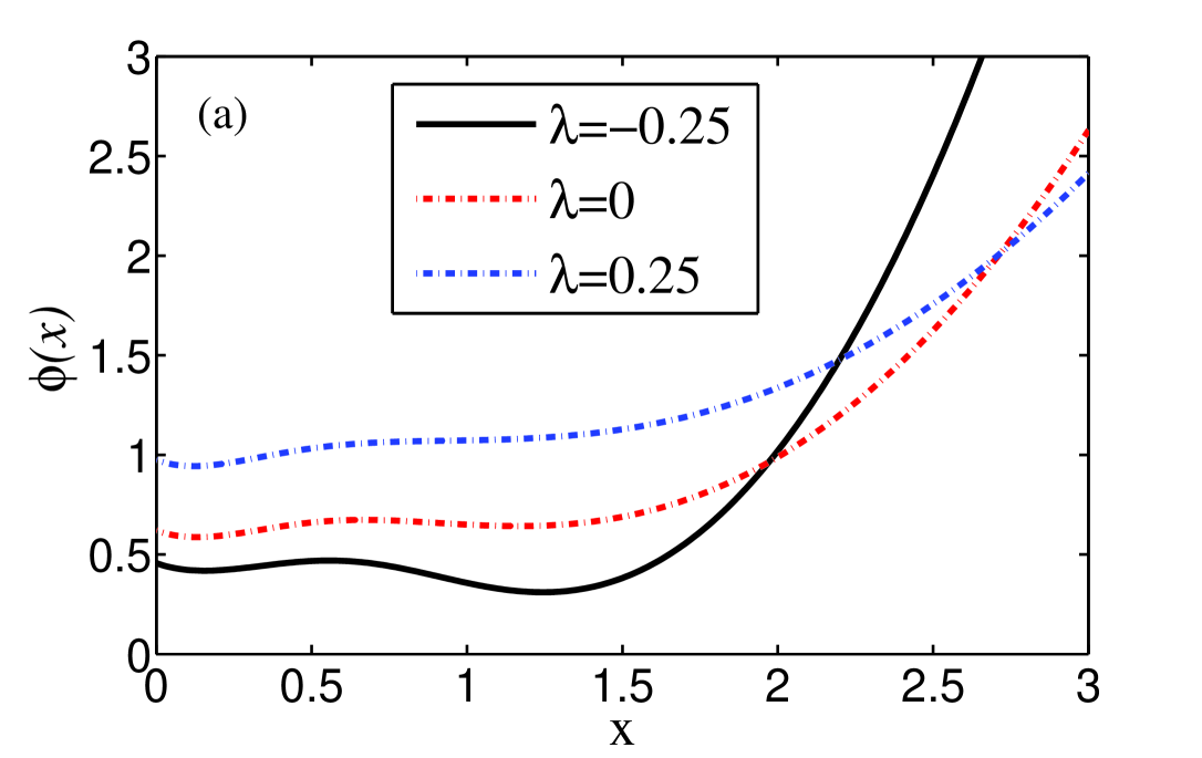
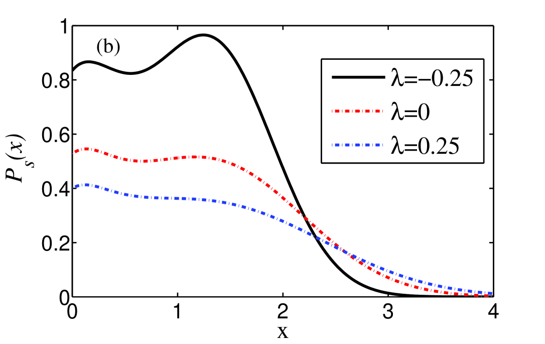
The expressions of the SPDF $P_{s}(x)$ and the potential $\phi(x)$ are given in Eq. (LABEL:Eq:SPDF1) and Eq. (9), respectively. Figure 7 shows the results for $\phi(x)$ and $P_{s}(x)$ for three different strengths of correlation between additive and multiplicative noise. The system parameters $r$ and $a$ are chosen in such a way that the deterministic system retains bistability. As we vary the correlation parameter $\lambda$ from a negative value to a positive value, it is evident from Fig. 7(a) that the resilience of right potential well is more sensitive with the change in $\lambda$ than that of left potential well. In fact, negative correlation ($\lambda<0$) will increase the stability of the high concentration of protein and positive correlation ($\lambda>0$) will increase the stability of the low concentration of protein (see the SPDF in Fig. 7(b)). Hence, an increase in the cross correlation intensity always induces regime shifts from high to low protein concentration state.

III.2 Mean first-passage time

In biological systems, where noise plays an important role in determining the dynamics, it is of general interest to calculate the robustness of the system steady state under perturbative condition. The robustness of a steady state can be quantified by the mean first-passage time (MFPT) in noise driven systems Ga09 ; Dr07 . In the bistable potential of Eq. (II.2), let $x^{st}_{l}/x^{st}_{u}$ $(x^{st}_{l}<x^{st}_{u})$ be the two steady states corresponding to the low/high protein concentrations separated by the potential barrier $x^{un}_{b}$ (i.e., the unstable equilibrium point). An equilibrium point can exit from its potential well in the presence of noise. The exit time is a number which depends on the specific realization of the random process and is known as first passage time. When the first passage time is averaged over many realizations, we get the mean first passage time.

Figure 8: (a) The logarithmic value of MFPT with an increase in $a$. The other parameter values are $r=0.1$, $\sigma_{1}=0.2$, $\sigma_{2}=0.9$ and $\lambda=0.01$. (b) The logarithmic value of MFPT with an increase in $\lambda$. The parameter values are $r=0.1$, $a=1.9$, $\sigma_{1}=0.4$ and $\sigma_{2}=0.9$.

In the context of anticipating regime shifts, MFPT provides a very useful characterization of the time scale on which a critical transition is likely to happen. When the structure of a dynamical system is known, the early warning signal indicators of regime shifts should be measured from the time series data of length shorter than the MFPT of the state in that particular regime.

Figure 9: Plot of the ratio $\gamma=\frac{T(x^{st}_{u})}{T(x^{st}_{l})}$ of the MFPT with respect to the control parameter $a$. The other parameter values are $r=0.1$, $\sigma_{1}=0.4$ and $\sigma_{2}=0.9$ and $\lambda=0.1$.

(a)	(b)	(c)

Figure 10: Early warning signals for simulated time series data of the stochastic model in the case of critical slowing down. We calculated variance and autocorrelation within rolling window of half the length of the time series segment (a segment is indicated by shaded region): (a) Additive noise: parameter values are $r=0.1$, $\sigma_{1}=0$ and $\sigma_{2}=0.9$; (b) Multiplicative noise: parameter values are $r=0.1$, $\sigma_{1}=0.9$ and $\sigma_{2}=0$; and (c) Correlated noise: parameter values are $r=0.1$, $\sigma_{1}=0.4$, $\sigma_{2}=0.1$ and $\lambda=0.5$. See text for more details.

It is clear that the basin of attraction of the state $x^{st}_{u}$ extends from $x^{un}_{b}$ to $+\infty$, as it is in the right of $x^{st}_{l}$. Let $T(x)$ be the MFPT to state $x^{un}_{b}$ starting at $x>x^{un}_{b}$. Then $T(x)$ satisfies the following ordinary differential equation Ga09 :

$$A(x)\frac{\partial T(x)}{\partial x}+\frac{1}{2}B(x)\frac{\partial^{2}T(x)}{\partial x^{2}}=-1,$$ (16)

with boundary conditions $T(x^{un}_{b})=0$ and $\frac{\partial T(+\infty)}{\partial x}=0$. Similarly one can calculate the MFPT to state $x^{un}_{b}$ for the basin of attraction of the state $x^{st}_{l}$ which extends from $0$ to $x^{un}_{b}$. After solving Eq. (16), one can obtain the MFPTs as Ga09 :

$$T(x^{st}_{l}) = 2\int_{x^{st}_{l}}^{x^{un}_{b}}\frac{1}{\psi(y)}dy\int_{0}^{y}\frac{\psi(z)}{B(z)}dz,\;\mbox{and}$$

$$T(x^{st}_{u}) = 2\int_{x^{un}_{b}}^{x^{st}_{u}}\frac{1}{\psi(y)}dy\int_{y}^{\infty}\frac{\psi(z)}{B(z)}dz,$$

where

$$\psi(x)=\exp\left(\int_{x_{0}}^{x}\frac{2A(x^{\prime})}{B(x^{\prime})}dx^{\prime}\right),$$

with $x_{0}=0$ for the $x^{st}_{u}\rightarrow x^{st}_{l}$ transition and $x_{0}=x^{un}_{b}$ for the $x^{st}_{l}\rightarrow x^{st}_{u}$ transition.

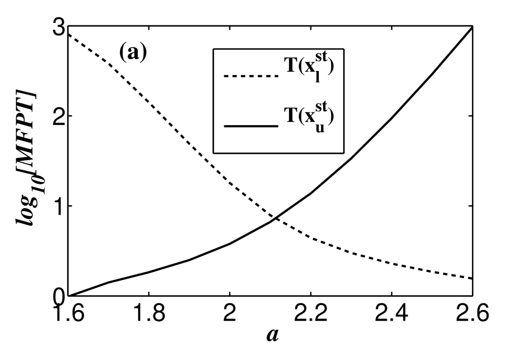
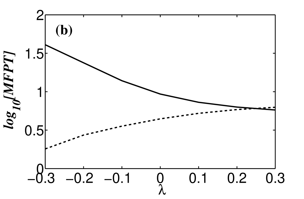
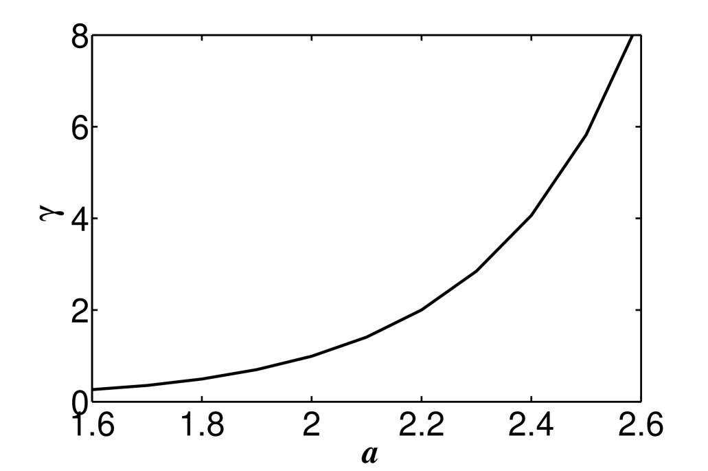
The effect of changing $a$ and also the correlation parameter $\lambda$ on the MFPT are shown in Fig. 8 (for the details of parameter values see the caption of Fig. 8). We can observe that the MFPT $T(x^{st}_{l})$ decreases and $T(x^{st}_{u})$ increases with an increase in $a$ (see Fig. 8(a)) and the opposite trend is observed for an increase in $\lambda$ (see Fig. 8(b)). These also imply the fact that an increase in $a$ promotes the regime shift from left potential well to the right potential well and vice versa for an increase in $\lambda$. As MFPT $T(x^{st}_{l})$ approaches to zero at the bifurcation point, the system loses its stability at low protein concentration. The asymmetry in the exit time is calculated by the ratio $\gamma=\frac{T(x^{st}_{u})}{T(x^{st}_{l})}$ and it diverges at the bifurcation point where $T(x^{st}_{l})$ approaches to zero (see Fig. 9) Ga09 . The quantity $\gamma$ thus gives an early warning signal of regime shifts from low to high protein concentration state for an increase in $a$.

III.3 Early warning signals

(a)	(b)	(c)

Figure 11: Early warning signals for simulated time series data of the stochastic model in the case of stochastic switching. Here also we calculated variance and autocorrelation within rolling window of half the length of the time series segment (a segment is indicated by shaded region): (a) Additive noise: parameter values are $r=0.1$, $a=2.1$, $\sigma_{1}=0$ and $\sigma_{2}=0.9$; (b) Multiplicative noise: parameter values are $r=0.1$, $a=2.3$, $\sigma_{1}=0.9$ and $\sigma_{2}=0$ and (c) Correlated noise: parameter values are $r=0.1$, $a=2.1$, $\sigma_{1}=0.4$, $\sigma_{2}=0.65$ and $\lambda=0.5$. See text for details.

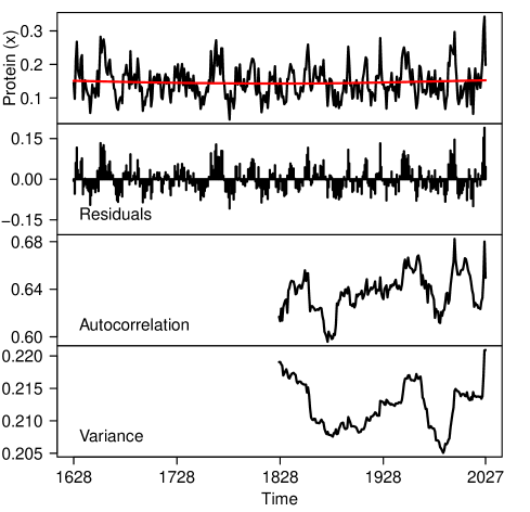
Here we assess the robustness of early warning signals to forewarn upcoming shifts to an alternative regime by analyzing simulated time series data Dakos:2012pone ; Kefi:2014pone from the considered stochastic model of genetic regulation. The simulation approach is showing how the characteristics captured in our analytical calculations can also be seen within individual time series realizations based on specific parameter sets. Early warning signals are observable statistical signatures that antecede some state shifts. These signals have mainly been derived from the phenomenon of critical slowing down (CSD) which arises in the vicinity of bifurcation wherein its dominant eigenvalue will cross zero Scheffer:2012sc . As the eigenvalue reduces to zero, the response of the system becomes very slow in recovering from perturbations and certain statistical features, such as increased variance and lag-$1$ autocorrelation, are predicted to appear in the time series analysis as a result (reviewed in Scheffer et al. ScJo09 ). Although many regime shifts appear as sudden transitions to another state in natural systems, the actual fact that not all regime shifts are associated with a bifurcation Boettiger:2013br ; DaCa15 . Hence not all regime shifts associated with different mechanisms are expected to exhibit CSD. In Dakos et al. DaCa15 , it is pointed out that CSD based early warning signals “are not a panacea for anticipating all types of regime shifts”.

Below we present two mechanisms those are responsible for observable regime shifts in our simulated time series. One is associated with the saddle-node bifurcation and exhibits CSD and another is associated with stochastic switching (SS) (i.e., purely noise-induced transition and not associated with bifurcation) and does not exhibit CSD. There has been a recent debate about the success of early warning signals for predicting stochastic switching induced regime shifts Drake:2013cb ; Boettiger:2013jc . Keeping that in mind, we felt that it is worthwhile to present what occurs in our system. For our analyses, we consider three different stochastic time series, each for CSD and SS: first we consider the presence of additive noise only, second we consider the presence of multiplicative noise only and finally presence of both noises with correlation in the system. To obtain the time series, stochastic simulations were performed in MATLAB (R2011a) using the Euler-Maruyama method DH01 and a standard integration step-size of 0.001.

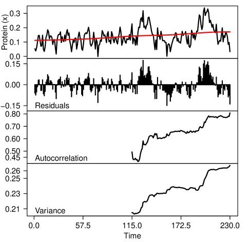
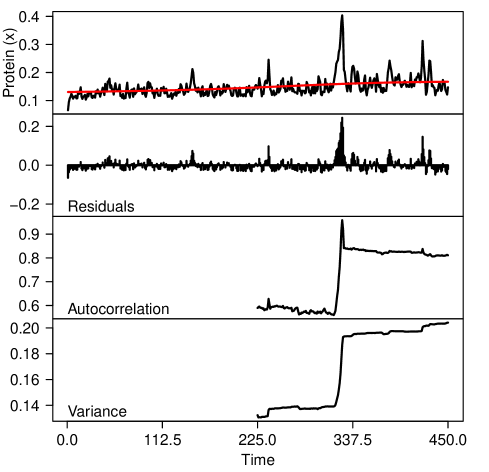
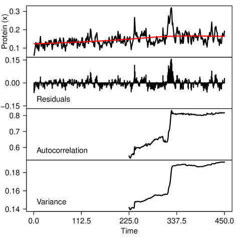
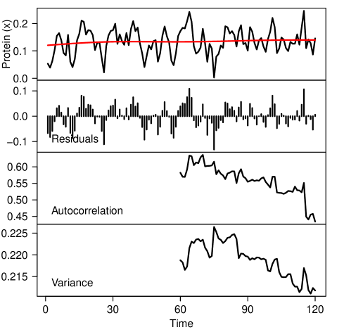
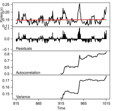
In our simulated time series, we visually identify shifts between low to high protein concentration and vice versa for both the cases, CSD and SS (see Figs. 10 and 11). Then we took different time series segments (the gray shaded regions in Figs. 10 and 11) of different lengths (keeping in mind that their time lengths should be less than their MFPTs) preceding a regime shift and analyzed those time series for the presence of early warning signals. The “Early Warning Signals Toolbox” (http://www.early-warning-signals.org/) is used to perform the statistical analyses. To ensure stationarity in residuals, we used Gaussian detrending with bandwidth 40, on the time series data before performing any statistical analysis. Then using a moving window size of half the length of the considered time series (i.e., $50\%$ of the considered time series segment), we calculate the variance and autocorrelation in our state variable, $x$, as these two indicators are both very commonly applied to anticipate regime shifts. The autocorrelation at lag-1 is measured by the autocorrelation function (ACF):

$$\rho_{1}=\frac{E[(x(t)-\mu)(x(t+1)-\mu)]}{\sigma^{2}},$$

where $x(t)$ is the value of the state variable at time $t$, and $\mu$ and $\sigma^{2}$ are the mean and variance of $x(t)$. Variance is the second moment around the mean $\mu$ and measured as:

$$\sigma^{2}=\frac{1}{N}\sum_{i=1}^{N}(x(t)-\mu)^{2},$$

where $N$ is the number of observations within the considered time frame. A concurrent increase in both of these indicators forewarn an impeding regime shift Scheffer:2012sc .

In Table I, we summarize results of early warning signals (see Figs. 10 and 11) for the considered two different cases of regime shifts with three subcases each. The signals [variance ($\sigma^{2}$) and autocorrelation ($\rho_{1}$)] are indicated as “$+$” if there is a concurrent rise; indicated as “$+/-$” if there is a rise, but some false pick in the signals before the regime shift due to the presence of large fluctuations in the data; and indicated as “$-$” if looking at the signals, it is not possible to forewarn an impending regime shift.

Table 1: Two mechanisms, CSD and SS that can produce regime shifts with and without bifurcation in the system and the outcome of early warning signals for regime shifts.

CSD                     SS
Noise Type      Var($\sigma^{2}$)   ACF($\rho_{1}$)   Var($\sigma^{2}$)   ACF($\rho_{1}$)
Additive	+	+	$-$	$-$
Multiplicative	+	+/$-$	+	+
Correlated:
Additive and	+	+/$-$	$-$	$-$
multiplicative

The result in Table I shows that in the case of CSD with all three different types of stochasticity applied to model (II.2), the variance is robust and always successfully predict upcoming regime shifts for all the three types of noise. However, the lag-1 autocorrelation is only successful to predict regime shifts for the case of additive noise only and can’t predict very positively an upcoming regime shift for multiplicative and correlated noise. This establishes the fact that even for the case of CSD the variance is more robust than autocorrelation in detecting regime shifts in genetic regulation and it is line with the findings in Da12 . For SS, both of the early warning signals are not very successful in detecting regime shifts. Using the EWS indicators it is not possible to detect upcoming regime shifts for additive and correlated noises (see Fig. 11). However, in the presence of multiplicative noise, the early warning signals give positive results. This is indeed a nice result given the fact that early warning signals are not developed for noise induced transitions, but rather for CSD which is associated with bifurcations. Nevertheless, our results show that even for the case of CSD though the EWS somewhat gives positive results, still some regime shifts may not be triggered by a concurrent rise in variance and autocorrelation. This is due to the fact these CSD indicators are reliable for specific systems and also have some key limitations DaCa15 . Like, there is false positive and false negative errors in data SKP14 . Some other limitations include size of the window which varies across the literature and how much data are required for analyzing EWS is still not clear. Moreover, variance is a robust indicator as compared to autocorrelation in the case of CSD and this is due to the fact that autocorrelation is affected by the length of time series (see Appendix S2 for more details) and more sensitive to false alarms. In the case of stochastic switching, anticipating regime shifts is more difficult due to sudden transitions. The significance of these findings are discussed in the discussion section below.

IV Discussion

In this paper, we investigated a stochastic genetic regulatory circuit using analytical techniques and numerical simulation to anticipate regime shifts in protein concentration. In this respect, we derived an approximate Fokker-Planck equation from the Langevin equation. We studied the effects of intensity of both the additive and multiplicative external noise and their correlation on the gene regulatory system. The present study suggests that the presence of additive noise in the system induces regime shifts from a low protein concentration to a high protein concentration state, whereas multiplicative noise induces regime shifts from a high to a low protein concentration state. Moreover, we also show that how a correlation between the additive and multiplicative noise is important in determining regime shifts and hence can regulate the production of protein levels. Furthermore, an increase in the cross correlation intensity from a negative to a positive value between the two noises induce regime shifts from high to low protein concentration state. Here we have also computed the robustness of steady states using the MFPT Ga09 . Our MFPT result uncovers the fact that an increase in MFPT of right potential well with the maximum production rate promotes regime shifts from left potential well to the right potential well and vice versa for an increase in the cross correlation intensity.

In addition, we used a recently developed tool (http://www.early-warning-signals.org/) of early warning signals to anticipate regime shifts in the considered gene regulatory system using simulated time series data for both the CSD and SS. Extensive literature on regime shifts is available for ecosystems, financial markets, climatic shifts, etc. However, to the best of our knowledge, there is very less work available on anticipating regime shifts in many areas of developmental biology, specifically in genetic regulation ChLi12 ; Ya14 . Here for the first time, for a genetic regulatory system, we used the time series analysis based EWS approach to predict upcoming regime shifts. As anticipated by some previous authors Drake:2013cb ; Boettiger:2013jc , we also find that the EWS of raising variance and autocorrelation are in general sensitive to false alarms and not always successful to reliably predict impending state shifts in our model. We found that the EWS are moderately more successful when we analyzed time series data in advance to a state shift in the case of CSD, whereas in the case of SS, it is specific to particular noise only. We observed some key limitations and statistical issues of EWS, such as false pick in data, size of the window and length of time series data. For our model, we also verified that rising variance appears as a robust indicator of CSD as compared to lag-$1$ autocorrelation. This is mainly due to the fact that autocorrelation is sensitive to the length of time series. For accurate estimation of autocorrelation, we need long and equidistant time series data which are not always available for real systems. However, variance is insensitive to this effect and as a result, measuring autocorrelation as EWS may increase the possibility of false alarms. While testing EWS to our simulated time series data, we also observed that selection of window size is another major problem for getting a positive signal of regime shifts. In the case of SS, anticipation of regime shifts is extremely difficult because a bifurcation point is neither approached nor crossed and there is suddenly a phase transition.

Anticipating regime shifts in gene regulatory system (aka in protein concentration level) can be useful to prevent disease onset and progression which may intercept unacceptable sudden transitions from a healthy state to a disease state TrAn15 . Examples of such regime shifts are asthma attacks, epileptic seizures and sudden deterioration of complex diseases ChLi12 ; gl15 ; TrAn15 . A well documented example of regime shift is type 1 diabetes (T1D) which is a form of diabetes mellitus LiLiZh2013 . T1D is a chronic inflammatory disease caused by insufficient production of insulin by $\beta$ cells in the pancreas. The genetic association of T1D is that the production of insulin through $\beta$ cells depends on HLA-encoding genes NoEr12 . If T1D associated genes are in “on” expression state, then $\beta$ cells produce insulin and releases insulin into the blood stream, but if they are in “off” expression state $\beta$ cells fail to produce insulin which leads to T1D. Prediction of regime shifts in gene expression using EWS from normal (“on”) to diabetic (“off”) state could prevent the switch to diabetic state and help to maintain the level of insulin.

In summary, our work reveals that stochasticity can have diverse complex effects on genetic regulatory systems. Early warning signals to anticipate forthcoming regime shifts in gene expression requires special attention to the underlying various statistical issues and limitations. In addition, to select a suitable window size and data length raise further difficulties. The main challenge of detecting early warning signals includes risk of false alarms and failed detections. One needs a deeper understanding of early warning signals of regime shifts, and how a balance between early warning signals and false alarms is achieved, will lead to important new insights in genetic regulation. Moreover, our results establish the important fact that finding a more robust indicator of regime shifts in complex natural systems is still in its infancy and demands extensive research. We hope that this study may also increase the interest among researchers to find a more robust indicator for detecting upcoming sudden transition in much broader class of systems in developmental biology.

Supporting Information

Appendix S1   Derivation of Stationary Probability Density Function.   (PDF)

Appendix S2    Additional examples of early warning signals.   (PDF)

Author Contributions

Conceived and designed the experiments: YS  PSD. Performed the experiments: YS  PSD. Analyzed the data: YS  PSD. Contributed reagents/materials/analysis tools: YS  PSD  AKG. Wrote the paper: PSD  YS.

References

- (1) M. Scheffer, S. R. Carpenter, J. A. Foley, C. Folke, and B. Walker. Catastrophic shifts in ecosystems. Nature, 413:591–596, 2001.
- (2) M. Rietkerk, S. C. Dekker, P. C. de Ruiter, and J. van de Koppel. Self-organized patchiness and catastrophic shifts in ecosystems. Science, 305(5692):1926–1929, 2004.
- (3) V. Dakos and J. Bascompte. Critical slowing down as early warning for the onset of collapse in mutualistic communities. Proceedings of the National Academy of Sciences USA, 111(49):17546–17551, 2014.
- (4) T. M. Lenton, H. Held, E. Kriegler, J. W. Hall, W. Lucht, S. Rahmstorf, and H. J. Schellnhuber. Tipping elements in the earth’s climate system. Proceedings of the National Academy of Sciences USA, 105(6):1786–1793, 2008.
- (5) R. M. May, S. A. Levin, and G. Sugihara. Complex systems: Ecology for bankers. Nature, 451:893–895, 2008.
- (6) P. E. McSharry, L. A. Smith, and L. Tarassenko. Prediction of epileptic seizures: are nonlinear methods relevant? Nature Medicine, 9:241–242, 2003.
- (7) J. M. Fox and G. M. Whitesides. Warning signals for eruptive events in spreading fires. Proceedings of the National Academy of Sciences USA, 112(8):2378–2383, 2015.
- (8) M. Scheffer, S. R. Carpenter, T. M. Lenton, J. Bascompte, W. A. Brock, V. Dakos, J. van de Koppel, I. A. van de Leemput, S. A. Levin, E. H. van Nes, M. Pascual, and J. Vandermeer. Anticipating critical transitions. Science, 338:344–348, October 2012.
- (9) C. Boettiger and A. Hastings. No early warning signals for stochastic transitions: insights from large deviation theory. Proceedings of the Royal Society B: Biological Sciences, 280:20131372, 2013.
- (10) S. R. Carpenter and W. A. Brock. Rising variance: a leading indicator of ecological transition. Ecology Letters, 9:311–318, January 2006.
- (11) S. R. Carpenter, W. A. Brock, J. J. Cole, J. F. Kitchell, and M. L. Pace. Leading indicators of trophic cascades. Ecology Letters, 11:128–138, 2008.
- (12) V. Guttal and C. Jayaprakash. Changing skewness: an early warning signal of regime shifts in ecosystems. Ecology Letters, 11:450–460, May 2008.
- (13) M. Scheffer, J. Bascompte, W. A. Brock, V. Brovkin, S. R. Carpenter, V. Dakos, H. Held, E. H van Nes, M. Rietkerk, and G. Sugihara. Early-warning signals for critical transitions. Nature, 461:53–59, September 2009.
- (14) D. A. Seekell, S. R. Carpenter, and M. L. Pace. Conditional heteroscedasticity as a leading indicator of ecological regime shifts. The American Naturalist, 178:442–451, October 2011.
- (15) V. Dakos, S. R. Carpenter, W. A. Brock, A. M. Ellison, V. Guttal, A. R. Ives, S. Kéfi, V. Livina, D. A. Seekell, E. H. van Nes, and M. Scheffer. Methods for Detecting Early Warnings of Critical Transitions in Time Series Illustrated Using Simulated Ecological Data. PLoS ONE, 7:e41010, 2012.
- (16) S. Kéfi, V. Guttal, W. A. Brock, S. R. Carpenter, A. M. Ellison, V. Livina, D. A. Seekell, M. Scheffer, E. H. van Nes, and V. Dakos. Early Warning signals of ecological transitions: methods for spatial patterns. PLoS ONE, 9:e92097, 2014.
- (17) L. Glass. Dynamical disease: Challenges for nonlinear dynamics and medicine. Chaos: An Interdisciplinary Journal of Nonlinear Science, 25:097603, 2015.
- (18) V. Dakos, S. R. Carpenter, E. H. van Nes, and M. Scheffer. Resilience indicators: prospects and limitations for early warnings of regime shifts. Philosophical Transactions of the Royal Society B: Biological Sciences, 370:20130263, 2015.
- (19) J. M. Drake. Early warning signals of stochastic switching. Proceedings of the Royal Society B: Biological Sciences, 280:20130686, 2013.
- (20) M. Kaern, T. C. Elston, W. J. Blake, and J. J. Collins. Stochasticity in gene expression: from theories to phenotypes. Nature Reviews Genetics, 6:451–464, 2005.
- (21) H. Maamar, A. Raj, and D. Dubnau. Noise in gene expression determines cell fate in bacillus subtilis. Science, 317:526–529, 2007.
- (22) D. Angeli, Jr. J. E. Ferrell, , and E. D. Sontag. Detection of multistability, bifurcations, and hysteresis in a large class of biological positive-feedback systems. Proceedings of the National Academy of Sciences USA, 101:1822–1827, 2004.
- (23) P. Thomasa, N. Popović, and R. Grima. Phenotypic switching in gene regulatory networks. Proceedings of the National Academy of Sciences USA, 111:6994–6999, 2014.
- (24) E. M. Ozbudak, M. Thattai, H. N. Lim, B. I. Shraiman, and V. A. Oudenaarden. Multistability in the lactose utilization network of escherichia coli. Nature, 427:737–740, 2004.
- (25) M. Acar, A. Becksei, and A. van Oudenaarden. Enhancement of cellular memory by reducing stochastic transitions. Nature, 435:228–232, 2005.
- (26) B. Müller-Hill. The lac operon: a short history of a genetic paradigm”,. Walter de Gruyter, Berlin, Germany, 1996.
- (27) C. Trefois, P. M. Antony, J. Goncalves, A. Skupin, and R. Balling. Critical transitions in chronic disease: transferring concepts from ecology to systems medicine. Current Opinion in Biotechnology, 34:48–55, 2015.
- (28) L. Chen, R. Liu, Z-P. Liu, M. Li, and K. Aihara. Detecting early-warning signals for sudden deterioration of complex diseases by dynamical network biomarkers. Scientific Reports, 2:342, 2012.
- (29) P. E. McSharry, L. A. Smith, and L. Tarassenko. Prediction of epileptic seizures: are nonlinear methods relevant? Nature Medicine, 9:241–242, 2003.
- (30) I. A. van de Leemput, M. Wichers, A. O. J. Cramer, D. Borsboom, F. Tuerlinckx, P. Kuppens, E. H. van Nes, W. Viechtbauer, E. J. Giltay, S. H. Aggen, C. Derom, N. Jacobs, K. S. Kendler, H. L. J. van der Maas, M. C. Neale, F. Peeters, E. Thiery, P. Zachar, and M. Scheffer. Critical slowing down as early warning for the onset and termination of depression. Proceedings of the National Academy of Sciences USA, 111(1):87–92, 2014.
- (31) J. G. Venegas, T. Winkler, G. Musch, M. F. V. Melo, D. Layfield, N. Tgavalekos, A. J. Fischman, R. J. Callahan, G. Bellani, and R. S. Harris. Self-organized patchiness in asthma as a prelude to catastrophic shifts. Nature, 434:777–782, 2005.
- (32) X. Liu, R. Liu, X.-M. Zhao, and L. Chen. Detecting early-warning signals of type 1 diabetes and its leading biomolecular networks by dynamical network biomarkers. BMC Medical Genomics, 6(Suppl 2):S8, 2013.
- (33) Z. Cheng, F. Liu, X. Zhang, and W. Wang. Robustness analysis of celular memory in an autoactivating positive feedback system. FEBS Letters, 582:3776––3782, 2008.
- (34) A. Becksei, B. Seraphin, and L. Serrano. Positive feedback in eukaryotic gene networks: cell differentiation by graded to binary response. The EMBO, 20:2528––2535, 2001.
- (35) J. J. Tyson, K. C. Chen, and B. Novak. Sniffers, buzzers, toggles and blinkers: dynamics of regulatory and signaling pathways in the cell. Current Opinion in Cell Biology, 15:221––231, 2003.
- (36) Q. Liu and Y. Jia. Fluctuations-induced switch in the gene transcriptional regulatory system. Physical Review E, 70:041907, 2004.
- (37) D. Frigola, L. Casanellas, J. M. Sancho, and M. Ibañes. Asymmetric stochastic switching driven by intrinsic molecular noise. PLoS ONE, 7:e31407, 2012.
- (38) M. Weber and J. Buceta. Stochastic stabilization of phenotypic states: The genetic bistable switch as a case study. PLoS ONE, 7:e73487, 2013.
- (39) P. Smolen, D. A. Baxter, and J. H. Byrne. Frequency selectivity, multistability, and oscillations emerge from models of genetic regulatory systems. American journal of Physiology, 274:C531–C542, 1998.
- (40) J. Hasty, J. Pradines, M. Dolnik, and J. J. Collins. Noise-based switches and amplifiers for gene expression. Proceedings of the National Academy of Sciences, 97:2075–2080, 2000.
- (41) W. Horsthemke and R. Lefever. Noise-Induced Transitions. Springer, Berlin, 1984.
- (42) D. L. Nelson and M. M. Cox. Lehninger Principles of Biochemistry. W.H. Freeman & Company, New York, 5th edition, 2008.
- (43) H. Risken and T. Frank. The Fokker–Planck Equation: Methods of Solution and Applications. Springer, Berlin, 2nd edition, 1996.
- (44) C. W. Gardiner. Stochastic Methods: A Handbook for the Natural and Social Sciences. Springer Series in Synergetics. Springer–Verlag, Berlin, 4th edition, 2009.
- (45) K. L. S. Drury. Shot noise perturbations and mean first passage times between stable states. Theoretical Population Biology, 72:153–166, 2007.
- (46) C. Boettiger, N. Ross, and A. Hastings. Early warning signals: the charted and uncharted territories. Theoretical Ecology, 6:255–264, June 2013.
- (47) D. J. Higham. An algorithmic introduction to numerical simulation of stochastic differential equations. SIAM Review, 43(3):525–546, 2001.
- (48) V. Dakos, E. H. van Nes, P. D’Odorico, and M. Scheffer. Robustness of variance and autocorrelation as indicators of critical slowing down. Ecology, 93:264–271, 2012.
- (49) Y. Sharma, K. C. Abbott, P. S. Dutta, and A. K. Gupta. Stochasticity and bistability in insect outbreak dynamics. Theoretical Ecology, 8:163–174, 2015.
- (50) T. Yang, C. Zhang, C. Zeng, G. Zhou, Q. Han, D. Tian, and H. Zhang. Delay and noise induced regime shift and enhanced stability in gene expression dynamics. Journal of Statistical Mechanics: Theory and Experiment, 12:P12015, 2014.
- (51) J. A. Noble and H. A. Erlich. Genetics of type 1 diabetes. Cold Spring Harbor Laboratory Press, 2:a007732, 2012.