On the origin of the correlations between the accretion luminosity and emission line luminosities in pre-main sequence stars.

Abstract

Correlations between the accretion luminosity and emission line luminosities (L_acc and L_line) of pre-main sequence (PMS) stars have been published for many different spectral lines, which are used to estimate accretion rates. Despite the origin of those correlations is unknown, this could be attributed to direct or indirect physical relations between the emission line formation and the accretion mechanism. This work shows that all (near-UV/optical/near-IR) L_acc-L_line correlations are the result of the fact that the accretion luminosity and the stellar luminosity (L_∗) are correlated, and are not necessarily related with the physical origin of the line. Synthetic and observational data are used to illustrate how the L_acc-L_line correlations depend on the L_acc-L_∗ relationship. We conclude that because PMS stars show the L_acc-L_∗ correlation immediately implies that L_acc also correlates with the luminosity of all emission lines, for which the L_acc-L_line correlations alone do not prove any physical connection with accretion but can only be used with practical purposes to roughly estimate accretion rates. When looking for correlations with possible physical meaning, we suggest that L_acc/L_∗ and L_line/L_∗ should be used instead of L_acc and L_line. Finally, the finding that L_acc has a steeper dependence on L_∗ for T-Tauri stars than for intermediate-mass Herbig Ae/Be stars is also discussed. That is explained from the magnetospheric accretion scenario and the different photospheric properties in the near-UV.

1 Introduction

The disk-to-star accretion rate is one of the most important parameters driving the evolution of pre-main sequence (PMS) stars. However, it is difficult to directly measure the mass accretion rate, for which indirect empirical methods are necessary to estimate it. A widely used method exploits the fact that the accretion luminosity (L_acc) correlates with the luminosity of various emission lines (L_line). Despite the unknown origin of these correlations, they are being used to quickly estimate accretion rates. The L_acc–L_line empirical correlations have been derived using samples of PMS stars by comparing their accretion luminosities, mostly obtained from the UV excess and line veiling, with the emission line luminosity (see e.g. Muzerolle et al., 1998c; Herczeg & Hillenbrand, 2008; Dahm, 2008; Fang et al., 2009; Rigliaco et al., 2012, and references therein). Currently, dozens of near-UV – optical – near-IR spectral lines have been found to correlate with L_acc for classical T Tauri (TT) stars (for instance, the hydrogen Balmer and Paschen series, HeI, OI, NaID and CaII transitions, Br$\gamma$… etc; see e.g. Alcalá et al., 2014, AL14 hereafter). The correlations of the accretion luminosity with several of these lines have been extended both to the sub-stellar and the intermediate-mass Herbig Ae/Be (HAeBe) regimes (Mohanty et al., 2005; Rigliaco et al., 2011; Donehew & Brittain, 2011; Mendigutía et al., 2011, 2013a).

Apart from the observational effort involved to look for additional emission lines that could serve as accretion tracers, several investigations aim to provide physical links between some of the spectral transitions and the accretion process, which would explain the origin of the L_acc–L_line correlations. In a nutshell, either the lines are directly tracing the accreting region (e.g. Muzerolle et al., 1998a, b; Kurosawa et al., 2006; Rigliaco et al., 2015), or they trace the accretion indirectly, by probing the accretion-powered outflows and winds (e.g. Hartigan et al., 1995; Edwards et al., 2006; Kurosawa et al., 2011; Kurosawa & Romanova, 2012). The correlation with forbidden lines like [OI] (6300 $\AA{}$) exhibited by HAeBes (Mendigutía et al., 2011) is more difficult to explain, as this line is not identified with accretion/winds but rather with the surface layers of the circumstellar disks (Acke et al., 2005). A further challenge to the various explanations of the origin of the L_acc–L_line correlations is that the variations in the accretion rate as measured from the UV excess do not generally correlate with the observed changes in the line luminosities (Nguyen et al., 2009; Costigan et al., 2012; Mendigutía et al., 2011, 2013a). However, time delays between different physical processes could be present (Dupree et al., 2012).

On the other hand, the accretion luminosity is also found to correlate with the luminosity of the central star (L_∗). The L_acc–L_∗ correlation extends over $\sim$ 10 orders of magnitude in L_acc, and $\sim$ 7 orders of magnitude in L_∗, covering all optically visible young stars from the sub-stellar to the HAeBe regime (see e.g. Natta et al., 2006; Clarke & Pringle, 2006; Tilling et al., 2008; Mendigutía et al., 2011; Fairlamb et al., 2015, and references therein). Based on a statistical analysis, Mendigutía et al. (2011) tentatively suggested that the correlation between the accretion luminosity and the luminosity of several emission lines in HAeBe stars could be driven by the common dependence of both luminosities on the stellar luminosity.

The main goal of this paper is to demonstrate the equivalence of the L_acc–L_line and L_acc–L_∗ correlations. In particular, we aim to show that all (near-UV, optical and near-IR) L_acc–L_line correlations in PMS stars are driven by the relationship between the stellar luminosity and the accretion luminosity, and that therefore the accretion luminosity necessarily correlates with the luminosity of all spectral lines regardless of their physical origin. Section 2 introduces and partially re-analyses the L_acc–L_∗ correlation in PMS stars. Section 3 shows the expression that links the L_acc–L_∗ relationship with the L_acc–L_line correlations. The inter-dependence between both types of correlations is illustrated in section 4 using both synthetic data and observational data from the literature. Some implications from all the previous analysis are included in section 5. Finally, section 6 summarizes our main conclusions.

2 The L_acc–L_∗ correlation

A representative example of the empirical correlation between the accretion and stellar luminosities is shown in Fig. 1. It includes data from the literature for very low-mass TTs and sub-stellar objects/companions (log (L_∗/L_⊙) $<$ -1.25), TTs (-1.25 $<$ log (L_∗/L_⊙) $<$ 0.75), late-type HAeBes (0.75 $<$ log (L_∗/L_⊙) $<$ 2.25), and early type HAeBes (log (L_∗/L_⊙) $>$ 2.25). The sources belong to different star forming regions. The graph shows that L_acc increases with L_∗, with a relation steeper for the TTs than for the HAeBes.

According to Clarke & Pringle (2006) and Tilling et al. (2008), the upper bound of the L_acc–L_∗ correlation (L_acc $\sim$ L_∗) is the consequence of sample selection effects; the luminosity of most stars above that limit is dominated by accretion and these objects are in a younger, embedded phase without an optically visible photosphere. The lower bound (L_acc $\sim$ 0.01L_∗, mainly for objects with L_∗ $>$ L_⊙) is limited by accretion detection thresholds (symbols with vertical bars in Fig. 1). The physical origin of the L_acc–L_∗ correlation is the subject of active debate. This topic is not analysed here but we refer the reader to several related works (e.g. Padoan et al., 2005; Alexander & Armitage, 2006; Dullemond et al., 2006; Vorobyov & Basu, 2008; Ercolano et al., 2014). Instead, our contribution below deals with the observed change in the slope of the L_acc–L_∗ correlation between the TT and the HAeBe stars (Mendigutía et al., 2011; Fairlamb et al., 2015).

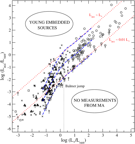
Figure 1: L_acc–L_∗ correlation for sub-stellar objects and TTs in different star forming regions (crosses; with vertical bars for upper limits; Natta et al., 2006; Herczeg & Hillenbrand, 2008, and references therein), four (sub-) stellar/planetary companions around PMS stars (squares; Close et al., 2014; Zhou et al., 2014), the Lupus sample from AL14 (dark triangles), and HAeBes (circles; with vertical bars for upper limits; Mendigutía et al., 2011; Fairlamb et al., 2015). The red diagonal dotted lines indicate L_acc = L_∗ and L_acc = 0.01L_∗. The three blue diagonal dashed lines represent the accretion luminosities expected from MA modelling for Balmer excesses of 0.70, 0.12 and 0.01 magnitudes (top, mid, and bottom lines, respectively). The vertical dotted line indicates the stellar luminosity at which the Balmer jump becomes apparent in the photospheric spectra (see also Fig. 2).

We constructed a sample of artificial stars representing the TT and HAeBe regime by using synthetic models of stellar atmospheres (Kurucz, 1993). The properties of each object are provided in Table 1. Columns two and three show the stellar luminosity and effective temperature. From these, the stellar radii was derived, spanning between 0.7 and 4 R_⊙ (column 4). The stellar masses (column 5) were derived assuming log g = 4, and cover the 0.2 – 6 M_⊙ range. Magnetospheric accretion (MA) shock modelling was carried out for each star by adding (blackbody) accretion contributions to the photospheric (Kurucz) spectra (see e.g. the reviews in Calvet et al., 2000; Mendigutía, 2013b). Two representative examples are presented in Fig. 2 (left panel). The shock model was applied following the usual recipes for both the TTs and HAeBes, and we refer the reader to Calvet & Gullbring (1998); Mendigutía et al. (2011) and Fairlamb et al. (2015) for further details. Three different values for the UV excess in the Balmer region of the spectra (from $\sim$ 3500 to 4000 $\rm\AA{}$, as defined in Mendigutía et al., 2013a) were modelled for each object assuming typical values for the inward flux of energy carried by the accretion columns (10¹² erg cm² s^-1) and the disk truncation radius (5R_∗): a ”maximum” excess (0.70 magnitudes), whose corresponding accretion contribution is L_acc $\sim$ L_∗ for L_∗ $\geq$ L_⊙; a ”minimum” excess (0.01 magnitudes) representative of the observational limit, and whose corresponding accretion contribution is L_acc $\sim$ 0.01L_∗ for L_∗ $\geq$ L_⊙; and finally, a ”typical” excess in-between the two previous (0.12 magnitudes). The resulting accretion luminosities are shown in the last three columns of Table 1. These are plotted versus the corresponding L_∗ values (blue diagonal dashed lines in Fig. 1), matching the overall distribution of data. We note that excesses larger than 0.70 magnitudes could still be measured for the less luminous sources (L_∗ $\leq$ L_⊙) without reaching the upper bound (L_acc $\sim$ L_∗).

Table 1: Sample of artificial stars. Stellar parameters and accretion luminosities from MA.

Star	L∗	T∗	R∗	M∗	(Lacc)m	(Lacc)t	(Lacc)M
$\sharp$	[log L⊙]	(K)	(R⊙)	(M⊙)	[log L⊙]	[log L⊙]	[log L⊙]
1	-1.25	3500	0.65	0.15	-4.85	-3.75	-2.84
2	-1.00	4000	0.66	0.16	-4.28	-3.17	-2.26
3	-0.75	4500	0.70	0.18	-3.64	-2.53	-1.61
4	-0.50	5000	0.75	0.20	-3.10	-1.99	-1.04
5	-0.25	5500	0.83	0.25	-2.62	-1.50	-0.53
6	0.00	6000	0.93	0.31	-2.20	-1.08	-0.08
7	0.25	6500	1.05	0.40	-1.85	-0.74	0.29
8	0.50	7000	1.21	0.53	-1.57	-0.45	0.58
9	0.75	7500	1.41	0.72	-1.36	-0.25	0.76
10	1.00	8000	1.65	0.99	-1.13	-0.02	0.98
11	1.25	8500	1.95	1.38	-0.89	0.22	1.21
12	1.50	9000	2.32	1.95	-0.64	0.47	1.46
13	1.75	9500	2.78	2.80	-0.40	0.72	1.71
14	2.00	10000	3.34	4.05	-0.15	0.97	1.96
15	2.25	10500	4.04	5.93	0.10	1.22	2.22

Notes. Columns two to five show the stellar luminosity (logarithmic scale, from the integrated Kurucz model atmospheres), effective temperature, stellar radius and mass. Columns six to eight show the MA accretion luminosities (logarithmic scale) corresponding to a minimum (m), typical (t) and maximum (M) Balmer excess of 0.01, 0.12 and 0.70 magnitudes, respectively.

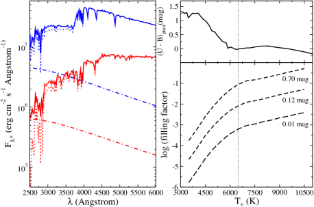
Figure 2: Left panel: MA modelling of a typical Balmer excess (0.12 magnitudes) for two representative stars with stellar temperatures of 7500 (blue) and 5500 $K$ (red). The photospheric (Kurucz) spectra, the contribution from accretion, and the total flux obtained from the combination of the previous are represented by the dotted, dot-dashed, and solid lines, respectively. The fluxes are as they would be measured at the stellar surface. Right panels: photospheric $U$ - $B$ colours (taken from Kenyon & Hartmann, 1995) characterizing the Balmer region of the spectrum (top) and filling factors necessary to reproduce a Balmer excess of 0.01, 0.12 and 0.70 magnitudes (bottom) using MA, versus the stellar temperature. The vertical dotted line indicates the stellar temperature at which the Balmer jump becomes apparent in the photospheric spectra (see also Fig. 1).

The fact that the accretion luminosity increases with the stellar luminosity is a natural consequence of MA shock modelling. This is illustrated in the left panel of Fig. 2. When the same excess (flux ratio between the solid and dotted lines) is observed in stars of different stellar luminosity, the most luminous stars (blue dotted line) must necessarily have a larger accretion contribution (dot-dashed lines). In order to understand the different slope in the L_acc –L_∗ correlation for TT and HAeBe stars, it is important to recall that the accretion contribution, and therefore L_acc, is proportional to both the temperature of the accretion columns (T_col) and the filling factor ($f$), which represents the fraction of the stellar surface covered by the accretion shocks. Variations in T_col and $f$ move the accretion-generated continuum excess along the wavelength axis and flux axis respectively. The typical value for T_col is $\sim$ 10⁴ $K$ across the TT and HAeBe regimes. Therefore, the excess peaks close to the Balmer region for both types of star. However, their photospheric spectra (i.e. when accretion is not present) are significantly different in that region. The Balmer jump becomes visible only for stars with log (L_∗/L_⊙) $\geq$ 0.25 (i.e. T_∗ $\geq$ 6500 $K$). This makes the spectra of stars with spectral types F and earlier more similar between them in the Balmer region than for later spectral types. Fig. 2 (top right panel) illustrates the case; the photospheric $U$-$B$ colour characterizing the Balmer region shows a steep dependence on the stellar temperature for cool stars, and flattens for hotter objects. Therefore, in order to reproduce a given Balmer excess, TTs require larger variations in the accretion luminosity than the ones that HAeBes need, for which the slope $\Delta$L_acc/$\Delta$L_∗ decreases from the TT to the HAeBe regime. The accretion luminosity changes are mainly affected by variations in the filling factor. This is shown in Fig. 2 (bottom right panel), where the filling factors that are needed to reproduce the minimum, typical and maximum model excesses are plotted against the stellar temperature. The change of slope in this panel occurs at the temperature where the Balmer jump appears ($\sim$ 6500 $K$), which corresponds to the stellar luminosity when the slope of the L_acc – L_∗ correlation changes (log (L_∗/L_⊙) $\sim$ 0.25). It is noted that we have applied basic MA modelling without considering aspects like the chromospheric contribution to the spectra of TT stars (Manara et al., 2013) or changes in the disk truncation radius depending on the stellar mass regime (Muzerolle et al., 2004; Mendigutía et al., 2011; Cauley & Johns-Krull, 2014). These factors could change the accretion estimates by less than 0.5 dex, without significantly affecting the modelled results in Figs. 1 and 2.

In summary, the observed difference in the L_acc–L_∗ correlation between TTs and HAeBes can be explained from the MA scenario and the differences in the near-UV stellar properties between both types of stars. However, we emphasize that the overall L_acc–L_∗ correlation is not a mere consequence of the MA shock modelling but most probably reflects a deeper physical relationship between both parameters (see e.g. the references at the beginning of this section). For example, the specific slopes shown by different samples in different environments (see e.g the Lupus sample with solid triangles in Fig. 1) cannot simply be explained from MA. Moreover, the L_acc–L_∗ correlation seems to arise also in embedded, younger sources, when the accretion luminosities are estimated from a variety of methods (Beltrán & de Wit, to be submitted). Regardless of the underlying physical origin of the L_acc–L_∗ correlation, for the rest of the paper it will be enough to remind that this arises whenever a significant sample of PMS stars is considered.

3 The accretion-stellar-line luminosity relation

The relation between the accretion and stellar luminosities is usually expressed in the literature as L_acc $\propto$ L${}_{*}^{b}$. This can also be written as a linear expression, which is a reasonable approach when the TT and HAeBe regimes are studied separately. For a given star, we will assume that L_acc and L_∗ can then be related by:

$$\log\left(\frac{L_{acc}}{L_{\sun}}\right)=a+b\times\log\left(\frac{L_{*}}{L_{\sun}}\right),$$ (1)

with $a$ and $b$ constants that depend on the star considered. When a sample of stars is studied, $a$ and $b$ represent the intercept and the slope of a linear fit to the data. This situation will be analysed in section 4.

The luminosity of a spectral line can be computed by multiplying the line equivalent width (EW) and the luminosity (per unit wavelength) of the adjacent continuum (L${}_{\lambda}^{c}$):

$$L_{line}=L_{\lambda}^{c}\times EW=\left(\frac{\alpha\cdot EW}{\beta}\right)\times L_{*},$$ (2)

with $\alpha$ the (dimensionless) excess of the (dereddened) continuum with respect to the photosphere at the wavelength of the line ($\alpha$ = $L_{\lambda}^{c}$/$L_{\lambda*}$ $\gid$ 1), and $\beta$ the ratio between the total stellar luminosity and the stellar luminosity at that wavelength ($\beta$ = L_∗/L_λ∗ $>>$ 1, in units of wavelength). The stellar luminosity in the second term of Eq. 2 was introduced in Eq. 1, obtaining:

$$\log\left(\frac{L_{acc}}{L_{\sun}}\right)=A+B\times\log\left(\frac{L_{line}}{L_{\sun}}\right),$$ (3)

which is again a linear expression, with:

$$\begin{split}&A=a-b\times\log\left(\frac{L_{line}}{L_{*}}\right);\\ &B=b,\end{split}$$ (4)

where L_line/L_∗ = $\alpha$EW/$\beta$, is the line to stellar luminosity ratio. Therefore, if the accretion luminosity of a given star can be derived from its stellar luminosity through Eq. 1, then the same accretion luminosity can be recovered from the luminosity of any emission line through Eqs. 3 and 4, with $A$ and $B$ constants that depend on the star and the line considered. Equations 1 and 3 are equivalent because both express a common dependence of the accretion luminosity on the stellar luminosity (Eq. 2).

4 The dependence of the L_acc–L_line correlations on the L_acc–L_∗ relation

In this section we use both synthetic and empirical data to illustrate the dependence of the L_acc–L_line correlations on the L_acc–L_∗ relation. Our first analysis provides a simple qualitative example on how the shape of the L_acc–L_∗ relationship has a strong effect on the L_acc–L_line correlations. We use the sample of artificial stars introduced in the previous section (see the first five columns of Table 1). The Kurucz models were used to calculate L${}_{\lambda}^{c}$ and $\beta$ at 6000 $\rm\AA{}$, whose values are presented in columns two and three of Table 2. Random EWs (between 1 and 10 $\rm\AA{}$, column four) are assigned to each object. These range in EW is representative of emission lines with intermediate strength such as the Ca II or OI transitions. The luminosity of an artificial emission line at 6000 $\rm\AA{}$ (column five) can then be obtained from Eqs. 2.

Table 2: Sample of artificial stars. Continuum and line properties.

Star	L${}_{6000}^{c}$	$\beta$($\lambda$ = 6000 $\rm\AA{}$)	EW	L6000
$\sharp$	[log L⊙ $\rm\AA{}$]	($\rm\AA{}$)	($\rm\AA{}$)	[log L⊙]
1	-5.64	24317	7	-4.79
2	-5.13	13363	5	-4.43
3	-4.74	9790	2	-4.44
4	-4.42	8343	9	-3.47
5	-4.14	7792	1	-4.14
6	-3.88	7573	2	-3.58
7	-3.63	7587	4	-3.03
8	-3.39	7698	7	-2.54
9	-3.15	7880	10	-2.15
10	-2.92	8284	3	-2.44
11	-2.69	8773	6	-1.91
12	-2.48	9603	8	-1.58
13	-2.27	10581	4	-1.67
14	-2.07	11723	1	-2.07
15	-1.86	12905	6	-1.08

Notes. Columns two to five list the luminosity of the continuum at 6000 $\rm\AA{}$ (logarithmic scale), the ratio between the total, star + accretion, luminosity and the stellar luminosity at 6000 $\AA{}$, a random EW of an hypothetical emission line assigned to each star (between 1 and 10 $\rm\AA{}$), and its corresponding luminosity at 6000 $\rm\AA{}$ (logarithmic scale).

The top left panel of Figure 3 shows two different L_acc–L_∗ linear relations assumed for the sample. Both have the same intercept but a different slope. The reverse is shown in the bottom left panel, in which the slope is kept constant and the intercept varies. The right hand panels show the corresponding accretion luminosities versus the luminosity of the artificial line at 6000 $\rm\AA{}$. The L_acc–L_line correlations follow the changes introduced in the L_acc–L_∗ relation, varying their slopes and intercepts. The range in the EW used only affects the scatter of the L_acc–L_line correlation, but this is ultimately determined by the L_acc–L_∗ relation. As introduced in section 3, the contribution of the continuum to the line luminosity dominates over the EW, and both the continuum and the accretion luminosities are correlated with the stellar luminosity. In order to illustrate this, the EW range was increased multiplying by 10 all the EWs $\geq$ 5 Å in column 4 of Table 2, and keeping the rest unmodified. This range in EW is representative of a strong emission line such as H$\alpha$. The new line luminosities are plotted with crosses in the bottom-right panel of Fig. 3, showing that for wider (narrower) EW ranges, the scatter in the L_acc–L_line correlation increases (decreases), but the correlation remains.

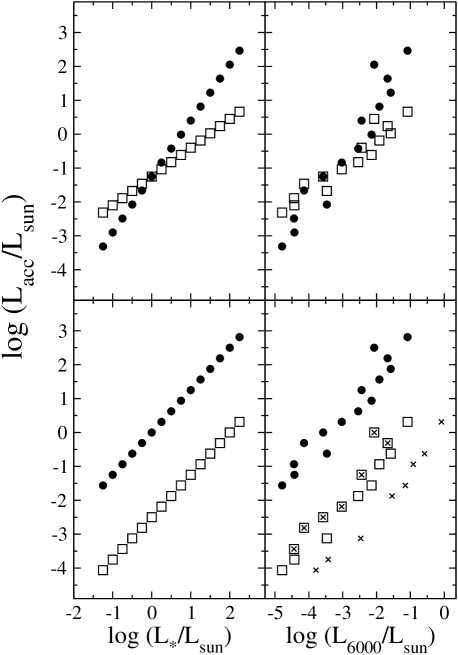
Figure 3: Results for the sample of artificial stars, showing how changes in the assumed L_acc–L_∗ correlation (left panels) have an effect on the L_acc–L_line relation (right panels) by changing the slope (top panels) and the intercept (bottom panels) of the former correlations. The crosses in the bottom-right panel represent the line luminosities obtained from a wider EW range, when the EWs $\geq$ 5 Å in column 5 of Table 2 are multiplied by a factor 10.

Before using real data from the literature to illustrate how the L_acc–L_line empirical correlations are driven by the L_acc–L_∗ relation, the equations described in the previous section have to be slightly modified. There, the values of L_acc were given by Eqs. 1 and 3, where $a$, $b$, $A$ and $B$ differ depending on the individual star and spectral line. In practice, the values for the slopes and intercepts of these equations are estimated using linear regression fitting, which provide unique $a$ and $b$ values for a given sample of stars, as well as unique $A$ and $B$ values for a given spectral line. In this case it can be shown (see Appendix A) that the slopes and intercepts of the L_acc–L_∗ and the L_acc–L_line empirical correlations are related by:

$$\begin{split}&A\sim a-b\times\epsilon\times\left<\log\frac{L_{line}}{L_{*}}\right>;\\ &B=b\times\epsilon;\\ &\epsilon=\frac{r_{line}\times\sigma_{*}}{r_{*}\times\sigma_{line}}\sim 1,\\ \end{split}$$ (5)

where $A$, $a$; $B$, and $b$ represent the intercepts and slopes of the L_acc–L_∗ and L_acc–L_line correlations, as derived from least squares linear regression fitting, $<$log L_line/L_∗$>$ the mean (logarithmic) line to stellar luminosity ratio, r_∗ and r_line the correlation coefficients of the L_acc–L_∗ and L_acc–L_line linear fits, and $\sigma$_∗ and $\sigma$_line the standard deviations of the log (L_∗/L_⊙) and log (L_line/L_⊙) values.

In short, when the empirical L_acc–L_∗ and L_acc–L_line correlations are compared, Eqs. 5 should be used instead of Eqs. 4. These are slightly modified by including the $\epsilon$ parameter, which accounts for the fact that the empirical correlations are in practice derived from (least-squares) linear fitting.

We use the observational data in AL14 to illustrate the dependence of the L_acc–L_line empirical correlations on the L_acc–L_∗ relation. These authors studied a sample of 36 low-mass TTs in the Lupus star forming region, for which they derived stellar parameters, accretion rates from the UV excess, and L_acc–L_line empirical correlations for dozens of emission lines in the spectral range from the near-UV to the near-infrared. To our knowledge, this work contains the largest number of spectral lines for which this type of correlations are derived. Another advantage is that for each star the accretion luminosity and the luminosity of all spectral lines were derived from the same spectrum, avoiding the problem of variability. In addition, all the stars are located at a similar distance, which guarantees that the correlations were not artificially stretched when the fluxes are multiplied by the squared distances to derive the (accretion and line) luminosities. Therefore, we consider the L_acc–L_∗ and L_acc–L_line correlations in AL14 as representative for similar correlations provided in the literature (see e.g the references in section 1).

The top panel of Fig. 4 shows the accretion and stellar luminosities of the stars studied by AL14. The observed trend is best fitted by log (L_acc/L_⊙) $\sim$ -1.3 + 1.4$\times$log (L_∗/L_⊙) (solid line). The slopes and intercepts of the L_acc–L_line empirical correlations derived by AL14 (see their table 4), which are exactly recovered by Eqs. 5, are plotted in the mid and bottom panels of Fig. 4 versus $\epsilon$ and $\epsilon$ $\times$ $<$log L_line/L_∗$>$, respectively. The mid panel shows that the slopes of the L_acc–L_line empirical correlations are a factor $\epsilon$ smaller than the slope of the L_acc–L_∗ correlation shown by the sample. As expected from Eqs. 5, the L_acc–L_line empirical correlations become steeper when $\epsilon$ increases, eventually reaching a slope of $\sim$ 1.4 for $\epsilon$ = 1. The bottom panel shows the expected linear decrease of the intercepts of the L_acc–L_line correlations with the ($\epsilon$-modified) line to stellar luminosity ratio. Equations 5 also imply that the typical (mean) slope of all L_acc–L_line correlations is given by the slope of the L_acc–L_∗ correlation of the sample, corrected by the mean value of $\epsilon$; $<$B$>$ = $b$ $\times$ $<$$\epsilon$$>$. Similarly, it can be derived that the mean intercept of the L_acc–L_line correlations is given by $<$A$>$ = $a$ - $b$ $\times$ $<$$\epsilon$ $\times$ $<$log L_line/L_∗$>$$>$. The two previous relations are also observed in the AL14 data, the mean values indicated with the dashed lines perpendicular to both axis in the mid and bottom panels of Fig 5.

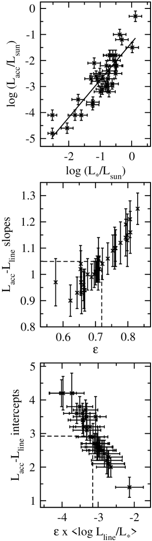
Figure 4: Based on results in AL14. Top panel: Accretion versus stellar luminosity. The best linear fit is log (L_acc/L_⊙) $\sim$ -1.3 + 1.4$\times$log (L_∗/L_⊙) (solid line). Mid and bottom panels: Slopes and intercepts of the L_acc–L_line empirical correlations versus the $\epsilon$ parameter (mid-panel) and the $\epsilon$-modified mean (logarithmic) line to stellar luminosity ratio (bottom-panel). The dashed lines indicate the mean values for the $x$ and $y$ axis, related from the slope and intercept of the top panel correlation by: $<$y$>$ = 1.4$<$x$>$ (mid panel), and $<$y$>$ = -1.3 - 1.4$<$x$>$ (bottom panel).

In summary, the analysis of both a sample of artificial stars and representative empirical data shows that the L_acc–L_line correlations are driven by the underlying L_acc–L_∗ relation shown by the sample of stars under study.

5 Consequences

The first consequence of the analysis in the previous sections is that the fact that PMS stars show the L_acc–L_∗ correlation immediately implies that L_acc also correlates with the luminosity of any (near-UV-optical-near-UR) emission line, regardless of the physical origin of the spectral transition. Indeed, it even correlates with the luminosity of a randomly general artificial emission line (right panels of Fig. 3). As mentioned earlier, the scatter of the L_acc–L_line correlations increases when the lines’ EWs exhibit a larger range. A similar effect occurs for stars with strong excess at short, UV, wavelengths and long, IR, wavelengths. For lines observed a these short and long wavelengths, the ratio $\alpha$EW/$\beta$ (i.e. the line to stellar luminosity ratio; Eq. 2) becomes significant, which could make the L_acc–L_line correlations much more scattered or eventually disappear.

For the other lines, the L_acc–L_line correlations are mainly determined by the L_acc–L_∗ dependence shown by the sample under analysis. The intercepts and slopes provided in the literature for the L_acc–L_∗ correlation ($a$ and $b$ in Eq. 1) vary depending on the sample of stars considered (Fairlamb et al., 2015, and references therein). Based on those works, a conservative observational limit is -2.5 $\leq$ $a$ $\leq$ 0, 0.8 $\leq$ $b$ $\leq$ 2. Consequently (see Eqs. 4 and 5), the slopes of all L_acc–L_line empirical correlations should also range in between $\sim$ 0.8 and 2, whereas the intercepts should all be $>$ 0 and decrease as the mean line to stellar luminosity ratio increases. These predictions agree with all L_acc–L_line published correlations based on observational data, to our knowledge. Interestingly, if two samples of stars show a different slope in their corresponding L_acc–L_∗ correlations, then the slopes of the L_acc–L_line ones are simply related via $B$’ $\sim$ $B$ $\times$ ($b$’/$b$) (assuming that the $\epsilon$ factors in Eq. 5 are roughly similar in both samples). This effect has already been observed. Mendigutía et al. (2011) reported a slight decrease in the slope of the L_acc–L_∗ correlation of a sample of 34 HAeBe stars with respect to TTs (see also Fig. 1 and Fairlamb et al., 2015). As discussed there, the slopes of the L_acc–L_line empirical correlations for the three lines studied (H$\alpha$, [OI] (6300 Å), and Br$\gamma$) also show a similar decrease.

That L_acc correlates with L_line is ultimately due to a common dependence of both luminosities on the stellar brightness. Because of this and the reasons above, the L_acc–L_line correlations alone cannot be seen as proof for either a direct or indirect physical connection between the spectral transitions and the accretion process. However, they are still useful expressions that can be applied to easily derive accretion luminosities without the need for sophisticated modelling of the UV excess. A basic measurement of a line luminosity suffices. Given that both observational L_acc–L_line and L_acc–L_∗ correlations show a roughly similar scatter (around $\pm$ 1 dex in L_acc), the latter can also be used to easily derive accretion rates from the stellar luminosity.

Analogously, since L_line necessarily correlates with L_∗ (Eq. 2), correlations between L_line and L_∗ alone can not be taken as a possible physical link between the spectral transition and the stellar luminosity (see also Natta et al., 2014). By extension, the luminosities of two different emission lines should also correlate with each other because of the common dependence on the stellar luminosity. Again, exceptions are possible for lines at short/long wavelengths in stars with strong excesses (see e.g. Meeus et al., 2012).

In order to infer from correlations possible physical links involving the luminosity of a spectral line or the accretion luminosity, it is necessary to get rid of the common dependence of both parameters on the stellar luminosity. This can be done by dividing L_line and L_acc by L_∗. Fig. 5 (top panels) shows the L_acc–L_line correlation for the sample of artificial stars from Table 2 and a given L_acc–L_∗ relation, and the intrinsic correlation between the stellar and line luminosities. However, the bottom left panels show that both L_acc/L_∗ and L_∗ do not correlate with L_line/L_∗, as expected from an artificial line created with random EWs. The right panels of the same figure show the results of the same exercise using real data from AL14. As expected, the H$\alpha$ luminosity correlates with both the accretion and stellar luminosities, which as we have discussed has no possible physical interpretation. In contrast with the previous example, in this case the H$\alpha$ line to stellar luminosity ratio is still correlated with the accretion to stellar luminosity ratio but not with the stellar luminosity itself, supporting the idea that this line is mainly driven by accretion and not by the stellar brightness.

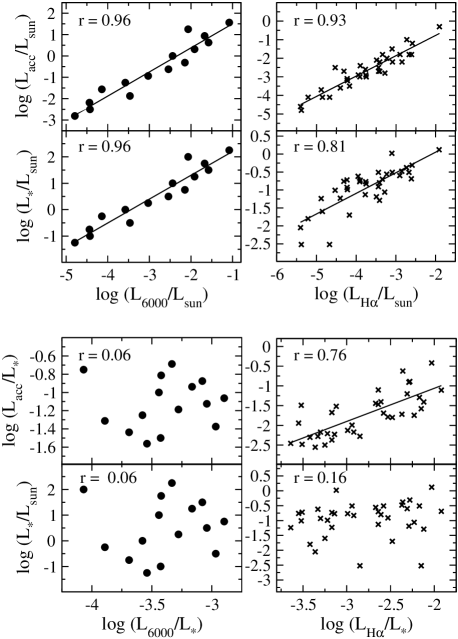
Figure 5: Comparison between different luminosities normalized by the solar and the stellar luminosity, as indicated in the axes’ labels. The left panels refer to the sample of artificial stars in Table 2, and the right panels to real observations from AL14. Linear regression fits are overplotted for those cases with large enough correlation coefficients (r $>$ 0.50; r-values indicated in each panel).

With this perspective in mind, we have confirmed that all line luminosities provided in AL14 correlate with each other, as expected. We also have checked that when the line luminosities are normalized by the stellar luminosities, some correlations remain while others disappear, indicating the presence or absence of a physical link between the different spectral transitions. For example, for H$\alpha$ and Br$\gamma$ the correlation is not only between their line luminosities but also between their line to stellar luminosity ratios, suggesting a common physical origin for both transitions. In contrast, despite the fact that the luminosities of the HeII (4686 $\rm\AA{}$) and the CaII (8498 $\rm\AA{}$) lines correlate, their line to stellar luminosities do not show a significant correlation, suggesting a different physical origin.

Finally, when the general L_acc – L_∗ correlation analysed in section 2 is transformed into L_acc/L_∗ vs L_∗, no trend is shown either for the whole sample or for specific samples like the Lupus objects in AL14. The vast majority of the objects have 0.01 $\leq$ $L_{acc}$/L_∗ $\leq$ 1 (diagonal dotted lines in Fig. 1) for all stellar luminosity bins. The typical value of $L_{acc}$/L_∗ is 0.1, which corresponds to the modelled, typical Balmer excess of 0.12 magnitudes. For the less luminous sources (L_∗ $<$ L_⊙), smaller L_acc/L_∗ ratios can still be obtained from the same Balmer excess detection limit. As discussed in Sect. 2, this is the expected consequence of the MA scenario and the photospheric properties of the stars in the near-UV.

It is beyond the scope of this work to carry out a detailed study on physical correlations involving stellar, line, and accretion luminosities. Instead, we have provided several examples to suggest that correlation analysis aiming to infer physical consequences should use L_line/L_∗ and L_acc/L_∗ and not simply L_line and L_acc.

6 Summary and conclusions

The L_acc–L_∗ empirical correlation in PMS stars has been partially re-analysed taking into account the newly available accretion rates for HAeBes. Despite the physical origin of the L_acc–L_∗ correlation remains subject to debate, the observed change of slope from the TT to the HAeBe regime can be understood from the MA scenario and the near-UV photospheric properties of the stars.

We have shown that the fact that PMS stars show the L_acc–L_∗ correlation immediately implies that L_acc also correlates with the luminosity of any (near-UV, optical, near-IR) emission line, regardless of the physical origin of the spectral transition. The overall L_acc–L_line trends are mainly governed by the L_acc–L_∗ correlation shown by the sample of stars under analysis. In particular, the slopes of the L_acc-L_line empirical correlations should typically be between $\sim$ 0.8 and 2 for all spectral lines, which are the observational limits for the slope of the L_acc-L_∗ relation. The intercepts also depend on the L_acc–L_∗ correlation, all of which are $>$ 0 and increasing as the line to stellar luminosity ratio decreases.

Despite the fact that the L_acc–L_line correlations alone do not constitute an indication of any direct or indirect physical link between the spectral transitions and accretion, they are a useful tool to easily derive estimates of the accretion rates. The L_acc–L_∗ correlations can be used for the same purpose. Similarly, correlations between stellar and line luminosities, or between different line luminosities, do not indicate a physical relation between the parameters involved. Instead, we suggest that the line to stellar and accretion to stellar luminosity ratios should be used when investigating the possible physical origin of the various correlations.

Appendix A Relation between the L_acc–L_line and L_acc–L_∗ linear regression correlations

Consider a sample of $N$ stars for which measurements of accretion and stellar luminosities [log (L_acc/L_⊙)₁,…, log (L_acc/L_⊙)_N; log (L_∗/L_⊙)₁,…, log (L_∗/L_⊙)_N)] are available. A linear fit to the data provides an expression that links both variables through

$$\log\left(\frac{L_{acc}}{L_{\sun}}\right)=a+b\times\log\left(\frac{L_{*}}{L_{\sun}}\right),$$ (6)

with $a$ and $b$ constants representing the intercept and the slope, which from least-squares linear regression are given by

$$\begin{split}&b=r_{*}\times\left(\frac{\sigma_{acc}}{\sigma_{*}}\right);\\ &a=\left<\log\left(\frac{L_{acc}}{L_{\odot}}\right)\right>-b\times\left<\log\left(\frac{L_{*}}{L_{\odot}}\right)\right>,\end{split}$$ (7)

where r_∗ is the correlation coefficient ($\sim$ 1 for well correlated data), and $\sigma$_acc, $\sigma$_∗; $<$log L_acc/L_⊙$>$, and $<$log L_∗/L_⊙$>$ the standard deviations and the means of the log (L_acc/L_⊙)_i and log (L_∗/L_⊙)_i values, respectively.

Similarly, if for the same sample of stars there are additional measurements of the luminosity of a given emission line [log (L_line/L_⊙)₁,…, log (L_line/L_⊙)_N], then a linear fit provides

$$\log\left(\frac{L_{acc}}{L_{\sun}}\right)=A+B\times\log\left(\frac{L_{line}}{L_{\sun}}\right),$$ (8)

with $A$ and $B$ constants given by least-squares linear regression

$$\begin{split}&B=r_{line}\times\left(\frac{\sigma_{acc}}{\sigma_{line}}\right);\\ &A=\left<\log\left(\frac{L_{acc}}{L_{\odot}}\right)\right>-B\times\left<\log\left(\frac{L_{line}}{L_{\odot}}\right)\right>,\end{split}$$ (9)

where the correlation coefficient, standard deviations, and means now refer to the [log (L_acc/L_⊙)_i, log (L_line/L_⊙)_i] values.

The standard deviation $\sigma$_acc can be found in the expression for $b$ of Eq. 7, and then introduced in the expression for $B$ of Eq. 9, providing the expression relating the slopes of the L_acc – L_∗ and L_acc – L_line linear correlations:

$$\begin{split}&B=\epsilon\times b;\\ &\epsilon=\frac{r_{line}\times\sigma_{*}}{r_{*}\times\sigma_{line}}.\end{split}$$ (10)

On the other hand, the mean value $<$log L_acc/L_⊙$>$ can be found in the expression for $a$ of Eq. 7, and introduced in the expression for $A$ of Eq. 9. Also considering Eq. 10, the expression that relates both intercepts is:

$$A=a-b\times\epsilon\times\left[\left<\log\left(\frac{L_{line}}{L_{*}}\right)\right>-\left(\frac{1-\epsilon}{\epsilon}\right)\times\left<\log\left(\frac{L_{*}}{L_{\odot}}\right)\right>\right].$$ (11)

The third term could been neglected ((1 - $\epsilon$)/$\epsilon$ $\sim$ 0) compared with the two other terms in the previous equation.

References

- Acke et al. (2005) Acke, B., van den Ancker, M.E., Dullemond, C.P. 2005, A&A, 436, 209
- Alcalá et al. (2014) (AL14) Alcalá, J.M.; Natta, A.; Manara, C.F. et al. 2014, A&A, 561, A2
- Alexander & Armitage (2006) Alexander R.D. & Armitage P.J. 2006, ApJ, 639, L83
- Calvet & Gullbring (1998) Calvet, N., & Gullbring, E. 1998, ApJ, 509, 802
- Calvet et al. (2000) Calvet, N.; Hartmann, L.; Strom, S.E. 2000, Evolution of Disk Accretion, in Protostars and Planets IV, ed. V. Mannings, A.P. Boss, & S.S. Russell (University of Arizona Press, Tucson), 377
- Cauley & Johns-Krull (2014) Cauley, P.W. & Johns-Krull, C.M. 2014, ApJ, 797, 112
- Clarke & Pringle (2006) Clarke, C.J., Pringle, J.E. 2006, MNRAS, 370, L10
- Close et al. (2014) Close, L.M.; Follette, K.B.; Males, J.R. et al. 2014, ApLJ, 781, L30
- Costigan et al. (2012) Costigan, G.; Scholz, A.; Stelzer, B. et al. 2012, MNRAS, 427, 1344
- Dahm (2008) Dahm, S.E. 2008, AJ, 136, 547
- Donehew & Brittain (2011) Donehew, B., & Brittain, S. 2011, AJ, 141, 46
- Dullemond et al. (2006) Dullemond C.D.; Natta A.; Testi L. 2006, ApJ, 645, L69
- Dupree et al. (2012) Dupree, A.K.; Brickhouse, N.S.; Cranmer, S.R. et al. 2012, ApJ, 750, 73
- Edwards et al. (2006) Edwards, S.; Fischer, W.; Hillenbrand, L.; Kwan, J. 2006, ApJ, 646, 319
- Ercolano et al. (2014) Ercolano, B.; Mayr, D.; Owen, J.E.; Rosotti, G.; Manara, C.F. 2014, MNRAS, 439, 256
- Fairlamb et al. (2015) Fairlamb J.R.; Oudmaijer, R.D.; Mendigutía; I., Ilee; J.D., van den Ancker, M.E. 2015, MNRAS, accepted.
- Fang et al. (2009) Fang, M.; van Boekel, R.; Wang, W. et al. 2009, A&A, 504, 461
- Hartigan et al. (1995) Hartigan, P.; Edwards, S.; Ghandour, L. 1995, ApJ, 452, 736
- Herczeg & Hillenbrand (2008) Herczeg, G.J.; Hillenbrand, L.A. 2008, ApJ, 681, 594
- Kenyon & Hartmann (1995) Kenyon, S.J. & Hartmann, L. 1995, ApJS, 101, 117
- Kurosawa & Romanova (2012) Kurosawa, R.; Romanova, M.M. 2012 2012, MNRAS, 426, 2901
- Kurosawa et al. (2011) Kurosawa, R.; Romanova, M.M.; Harries, T.J. 2011, MNRAS.416, 2623
- Kurosawa et al. (2006) Kurosawa, R.; Harries, T.J.; Symington, N.H. 2006, MNRAS, 370, 580
- Kurucz (1993) Kurucz, R. L. 1993, synthe Spectrum Synthesis Programs and Line Data, Kurucz CD-ROM (Cambridge, MA: Smithsonian Astrophysical Observatory)
- Manara et al. (2013) Manara, C.F.; Testi, L.; Rigliaco, E. et al. 2013, A&A, 551, A107
- Meeus et al. (2012) Meeus, G.; Montesinos, B.; Mendigutía, I. et al. 2012, A&A, 544, A78
- Mendigutía et al. (2011) Mendigutía, I., Calvet, N., Montesinos, B. et al. 2011, A&A, 535, A99
- Mendigutía et al. (2013a) Mendigutía, I., Brittain, S., Eiroa, C. et al. 2013, ApJ, 776, 44
- Mendigutía (2013b) Mendigutía, I. 2013, AN, 334, 129
- Mohanty et al. (2005) Mohanty, S.; Jayawardhana, R.; Basri, G. 2005, ApJ, 626, 498
- Muzerolle et al. (2004) Muzerolle, J.; D’Alessio, P.; Calvet, N.; Hartmann, L. 2004, ApJ, 617, 406
- Muzerolle et al. (1998a) Muzerolle, J.; Calvet, N.; Hartmann, L. 1998a, ApJ, 492, 743
- Muzerolle et al. (1998b) Muzerolle, J.; Hartmann, L.; Calvet, N. 1998b, AJ, 116, 455
- Muzerolle et al. (1998c) Muzerolle, J.; Hartmann, L.; Calvet, N. 1998c, AJ, 116, 2965
- Natta et al. (2014) Natta, A.; Testi, L.; Alcalá, J.M. et al. 2014, A&A, 569, A5
- Natta et al. (2006) Natta, A.; Testi, L.; Randich, S. 2006, A&A, 452, 245
- Nguyen et al. (2009) Nguyen, D.C.; Scholz, A.; van Kerkwijk, M.H.; Jayawardhana, R.; Brandeker, A. 2009, ApJL, 694, L153
- Padoan et al. (2005) Padoan P.; Kritsuk A.; Norman M.; Nordlund, . 2005, ApJ, 622, L61
- Rigliaco et al. (2015) Rigliaco, E.; Pascucci, I.; Duchene, G. et al. 2015, ApJ, complete.
- Rigliaco et al. (2012) Rigliaco, E.; Natta, A.; Testi, L. et al. 2012, A&A, 548, A56
- Rigliaco et al. (2011) Rigliaco, E.; Natta, A.; Randich, S. et al. 2011, A&A, 526, L6
- Tilling et al. (2008) Tilling, I., Clarke, C.J., Pringle, J.E., Tout, C.A. 2008, MNRAS, 385, 1530
- Vorobyov & Basu (2008) Vorobyov, E.I. & Basu, S. 2008, ApJ, 676, L139
- Zhou et al. (2014) Zhou, Y.; Herczeg1, G.J.; Kraus, A.L.; Metchev, S.; Cruz, K.L. 2014, ApJL, 783, 1