A versatile numerical method for obtaining structures of rapidly rotating baroclinic stars: self-consistent and systematic solutions with shellular-type rotation

Abstract

This paper develops a novel numerical method for obtaining structures of rapidly rotating stars based on a self-consistent field scheme. The solution is obtained iteratively. Both rapidly rotating barotropic and baroclinic equilibrium states are calculated self-consistently using this method. Two types of rotating baroclinic stars are investigated by changing the isentropic surfaces inside the star. Solution sequences of these are calculated systematically and critical rotation models beyond which no rotating equilibrium state exists are also obtained. All of these rotating baroclinic stars satisfy necessarily the Bjerknes–Rosseland rules. Self-consistent solutions of baroclinic stars with shellular-type rotation are successfully obtained where the isentropic surfaces are oblate and the surface temperature is hotter at the poles than at the equator if it is assumed that the star is an ideal gas star. These are the first self-consistent and systematic solutions of rapidly rotating baroclinic stars with shellular-type rotations. Since they satisfy the stability criterion due to their rapid rotation, these rotating baroclinic stars would be dynamically stable. This novel numerical method and the solutions of the rapidly rotating baroclinic stars will be useful for investigating stellar evolution with rapid rotations.

1 Introduction

One of the most fascinating challenge in the stellar astrophysics is understanding the structures of realistic rotating stars and their evolution (for example, see Maeder & Meynet 2000; Langer 2012). According to recent observations, many stars display detectable rotations. In fact, massive stars in particular, such as B and O stars, tend to have clearly rapid rotation (e.g. Hunter et al. 2008). Approximately 10 per cent of them have the rotational velocities which are larger than 300 $\mathrm{km\,s^{-1}}$ (Ramírez-Agudelo et al. 2013; Dufton et al. 2013). Such rapid rotational velocities can reach the critical velocity beyond which mass shedding due to rotation occurs and no equilibrium state exists (Maeder 2009), because the typical values of the critical velocities for 20 $M_{\odot}$ star with solar metallicity are $\sim$ 300 $\mathrm{km\,s^{-1}}$ - 600 $\mathrm{km\,s^{-1}}$ during the main sequence phase (Ekström et al. 2008). The shape of these rapidly rotating stars is oblate due to the centrifugal force. Therefore, their outer layers cannot be well described by spherical models due to their fast rotation and so non-spherical models are required to describe them. The structures of realistic rotating stars are described by using many realistic physical properties and processes such as viscosity, inhomogeneous chemical composition and meridional flows (not considered in this paper). In general, the surfaces of equal density (isopycnic surfaces) and equal pressure (isobaric surfaces) do not coincide due to these physical properties and processes, i.e. the stars becomes baroclinic.

Fig. 1 displays two examples of rapidly rotating baroclinic stars. The isopycnic surfaces (solid curves) are inclined to the isobaric surfaces (dashed curves). The isopycnic surfaces are more oblate than the isobaric surfaces in the left model, while the isobaric surfaces are more oblate than the isopycnic surfaces in the right model. Therefore, the value of the density on the isobaric surface varies in the baroclinic star. On each isopycnic surface, the density in the left model increases from the pole to the equator, while the density in the right model decreases from the pole to the equator. These two models are different classes of baroclinic stars explained in detail in Sec. 2.1.

The baroclinicity is characterized by the angle between isopycnic surfaces and isobaric surfaces. It is assumed that the system is stationary and axisymmetric and the star does not have magnetic field and meridional flow, the Euler equation of the rotating star is

$$\frac{1}{\rho}\nabla p=-\nabla\phi+R\Omega^{2}\mbox{\boldmath$e$}_{R},$$ (1)

where $\rho$, $p$, $\phi$ and $\Omega$ are, respectively, the density, the pressure, the gravitational potential and the angular velocity of the star. Cylindrical coordinates ($R$, $\varphi$, $z$) are utilized in this equation. The $\varphi$ component of the curl of this equation is

$$\frac{1}{\rho^{2}}\left(\nabla p\times\nabla\rho\right)_{\varphi}=\dfrac{\partial R\Omega^{2}}{\partial z}.$$ (2)

If the isopycnic surfaces and the isobaric surfaces coincide, i.e. the pressure depends on the density only, the star is barotropic ($p=p(\rho)$) and the left-hand side of the equation vanishes. The rotation of the barotropic star is rigid ($\Omega=\Omega_{0}$, constant) or cylindrical ($\Omega=\Omega(R)$) because the centrifugal force can be derived from a rotational potential (e.g. Eriguchi & Mueller 1985; Hachisu 1986a, b; Maeder 2009; Fujisawa 2015) as

$$0=\dfrac{\partial R\Omega^{2}}{\partial z}\Rightarrow\nabla\phi_{\mathrm{r}ot.}=R\Omega^{2}(R)\mbox{\boldmath$e$}_{R},$$ (3)

where $\phi_{\mathrm{rot.}}$ is the rotational potential that is an arbitrary function of $R$. If the isopycnic surfaces are inclined to the isobaric surfaces, the left-hand side of equation (2) does not vanish. The angular velocity distributions in the baroclinic stars are no longer constant and cylindrical due to the differences between isopycnic surfaces and isobaric surfaces. The situation is completely different from baroclinic star. Therefore, baroclinicity is an important component to consider in order to investigate such realistic rotating stars and their evolution.

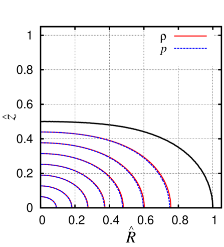
Figure 1: Seven arbitrary isopycnic surfaces (solid curves) and isobaric surfaces (dashed curves) of baroclinic rotating stars. The outermost curves denote the stellar surface. The isopycnic surfaces are more oblate than the isobaric surfaces in the left-hand panel, while the isobaric surfaces are more oblate than the isopycnic surfaces in the right-hand panel. These two models are different classes of baroclinic stars.

Nevertheless, only a few works have succeeded in obtaining baroclinic equilibrium states with rapid rotation self-consistently because it is difficult to calculate and analyse baroclinic stars. If it is assumed that the star is barotropic, the rotation becomes cylindrical and the centrifugal force can be derived from the potential in equation (3). Therefore, the first integral of the Euler equation can be obtained analytically as

$$\int\frac{dp}{\rho}=-\phi+\phi_{\mathrm{rot.}}+C,$$ (4)

where $C$ is the integral constant. Since the system is barotropic ($p=p(\rho)$), the integral of the left-hand side of this equation can be also calculated. This first integral of the Euler equation is used by many previous works for obtaining rapidly rotating barotropic stars (e.g. Eriguchi & Mueller 1985; Hachisu 1986a, b). In contrast, the situation of the baroclinic star is more complicated. If the star is baroclinic, the first integral of the Euler equation cannot be obtained analytically because the centrifugal force cannot be derived from a rotational potential and the distributions of the angular velocity must be calculated self-consistently by solving equation (2).

In order to avoid this difficulty, many previous works treated rotating baroclinic stars as slowly rotating stars by using perturbative methods (Roxburgh et al. 1965; Roxburgh & Strittmatter 1966; Faulkner et al. 1968; Clement 1969; Sackmann & Anand 1970; Kippenhahn & Thomas 1970; Monaghan 1971; Sharp et al. 1977). Others calculated self-consistent rotating equilibrium states, but treated rotating stars as pseudo-barotropic, i.e. isobaric surfaces and isopycnic surfaces are not inclined (Jackson 1970; Papaloizou & Whelan 1973; Eriguchi & Mueller 1991; Jackson et al. 2005). Although these studies considered the thermal balance of a rotating star in these works, the isothermal surfaces are also isobaric and so the system is essentially barotropic. Only a few works succeeded in obtaining rapidly rotating baroclinic stars self-consistently.

Uryu & Eriguchi (1994) investigated self-consistent rotating baroclinic equilibrium states. They discretized all basic equations of fully radiative stars and calculated them simultaneously by using Straight-Forward Newton-Raphson scheme (Eriguchi & Mueller 1985). The numerical code was extended by Uryu & Eriguchi (1995) and more realistic stars with a convective core and radiative envelope were calculated. Roxburgh (2006) obtained self-consistent rotating baroclinic stars with shellular rotation using an iterative method (Roxburgh 2004). Roxburgh (2006) did not adopt a particular equation of state and did not solve a thermal balance equation. Instead, both density and pressure distributions were obtained independently and calculated iteratively by fitting the radial profile of the angular velocity. Espinosa Lara & Rieutord (2007) succeeded in obtaining self-consistent rotating baroclinic stars with viscosity and meridional flows by using a pseudo-spectral method (cf. Rieutord 1987). In their numerical code, the physical variables are projected on to the spherical harmonics and solved iteratively via a generalized algorithm for polytropic stellar models (Bonazzola et al. 1998). More recently, the numerical code was improved and many realistic and complex solutions were obtained by Espinosa Lara & Rieutord (2013). Very recently, Yasutake et al. (2015) developed a new formulation and numerical method based on the Lagrangian variational principle to obtain rotating self-gravitating configurations. They were able to obtain both rotating barotropic and baroclinic equilibrium sates consistently by using their new method.

These studies have improved self-consistent rotating baroclinic models, but the basic understanding of rotating baroclinic stars is still unclear because there are only the few solutions of such stars that were developed in the aforementioned works. Many solution sequences and systematic studies are required to improve the understanding of rotating baroclinic stars and their evolution. Simple and powerful numerical methods are needed to systematically obtain solution sequences. As a first step towards realistic rotating stars and their evolution, this paper investigates a versatile numerical method for systematically obtaining structures of rapidly rotating baroclinic stars as well as solutions for baroclinic rotating stars. A simple equation of state is adopted in this paper in order to obtain rotating baroclinic stars easily and systematically. Some previous self-consistent works adopted complex thermal balance equations, but the rotating baroclinic equilibrium state itself is determined without any explicit thermal balance equation (Roxburgh 2006; Yasutake et al. 2015). The mechanical structures themselves are determined independently from assumed or additional thermal structures which are totally independently and freely introduced to mechanical structures in Newtonian gravity. It should be noted that the mechanical part and the thermal part cannot be separated in general relativistic situations because the total energy density is one of the source of the gravity in the Einstein equations (Yoshida et al. 2012). Therefore, in the Newtonian gravity framework, we can obtain rotating baroclinic stars systematically even when we ignore the thermal balance equation. This paper adopts a simple equation of state as a baroclinic equation of state, but a realistic equation of state could also be easily integrated into the method. This new method can calculate rapidly rotating baroclinic stars easily.

The remainder of this paper is organized as follows. Section 2 describes the formulation of the rotating baroclinic star and numerical scheme of the new method. Section 3.1 verifies the accuracy of the numerical results and compares them with results obtained via another numerical scheme. The numerical results and solution sequences are displayed in Section 3.2. Discussion is given in Sections 4.1 and 4.2. The paper is summarized in Section 4.3.

2 Formulation and numerical method

The formulation and details of the numerical method are described in this section. The formulation of rotating baroclinic stars is summarized in Section 2.1. The remainder of this section focuses on explaining the new numerical scheme briefly. Both spherical polar coordinates $(r,\theta,\varphi)$ and cylindrical coordinates $(R,\varphi,z)$ are utilized in the formulation, but spherical polar coordinates are employed in the actual numerical code.

2.1 A formulation of rotating baroclinic stars

It is assumed that the system is in a stationary state and the configuration is axisymmetric about the rotational axis. It is also assumed that the configuration is equatorially symmetric. Both meridional flow and magnetic field are neglected in this paper. Although the meridional flow plays important role for secular transport processes in stellar interiors (e.g. Mathis 2013), the typical time-scale of the meridional flow is much longer than the dynamical time-scale of the star. It is almost negligible to consider the mechanical structures of the rapidly rotating star in equilibrium. Under these assumptions, the basic equations that describe the rotating baroclinic star are the Euler equations

$$\frac{1}{\rho}\dfrac{\partial p}{\partial r}=-\dfrac{\partial\phi}{\partial r}+r\sin^{2}\theta\Omega^{2},$$ (5)

$$\frac{1}{\rho}\dfrac{\partial p}{\partial\theta}=-\dfrac{\partial\phi}{\partial\theta}+r^{2}\sin\theta\cos\theta\Omega^{2},$$ (6)

the integral form of the Poisson equation

$$\phi=-G\int\frac{\rho(\mbox{\boldmath$r$}^{\prime})}{|\mbox{\boldmath$r$}-\mbox{\boldmath$r$}^{\prime}|}d^{3}\mbox{\boldmath$r$}^{\prime},$$ (7)

and a baroclinic equation of state

$$p=p(\rho,X),$$ (8)

where $\rho$, $p$, $\phi$, $\Omega$, $G$, and $X$ are, respectively, the density, the pressure, the gravitational potential, the angular velocity, the gravitational constant and a scalar function that characterizes a baroclinicity such as temperature $T$ or specific entropy $s$. In this paper, the following analytic form of a simple equation of state is adopted:

$$p(\rho,K)=K(r,\theta)\rho^{1+1/N},$$

$$K(r,\theta)=K_{0}\left\{1+\epsilon\left(\frac{\sin^{2}\theta}{a_{0}^{2}}+\frac{\cos^{2}\theta}{b_{0}^{2}}\right)r^{m}\right\},$$ (9)

where $\epsilon$, $a_{0}$, $b_{0}$, $K_{0}$, $m$ are parameters. $K$ is related to the specific entropy of the star. If we assume the ideal gas star ($p\sim T\rho$), then $K$ is proportional to the specific entropy ($K\propto\exp(s)$) and the distribution of $K$ represents the distribution of the specific entropy. If the $K$ at the equator is lager than at the pole, the surface temperature is hotter at the equator than at the pole. If the $K$ at the equator is smaller than that at the pole the surface temperature is cooler at the equator than at the pole. Although this equation of state is simple, two types of rotating baroclinic stars in Fig. 1 are obtained by this equation of state. Spherical isentropic (constant entropy) and oblate isentropic models were investigated by fixing the values of $a_{0}$ and $b_{0}$ of this analytic form of $K$, noting that the isentropic surfaces becomes spherical when $a_{0}=b_{0}$ and oblate when $a_{0}>b_{0}$ respectively. The spherical isentropic model has the spherical isentropic surfaces and the oblate isentropic models has the oblate isentropic surfaces. These two types of isentropic models become two types of rotating baroclinic models in Fig. 1. The value of $\epsilon$ denotes the degree of baroclinicity. If we fix $\epsilon=0$, the system becomes barotropic since $K$ becomes constant and $p$ is a function of $\rho$ $(p=p(\rho))$. However, if we choose $\epsilon\neq 0$, then $K$ is no longer constant and the system becomes baroclinic. As the absolute value of $\epsilon$ increases, the baroclinicity of the star also increases. As we will see in Section 3, this simple equation of state systematically provides various rotating baroclinic stars by fixing the parameters in this ways. Since the isentropic surfaces are oblate in the oblate isentropic model, the $K$ at the equator is smaller than at the pole. Therefore, the surface temperature of the oblate isentropic model is hotter at the pole than at the equator. From a observational point of view, the surface temperatures of the rapidly rotating early type stars are hotter at the poles than that at the equator (e.g. $\alpha$ Leonis observed by Che et al. 2011) by the gravitational darkening (von Zeipel 1924). Therefore, the oblate isentropic model might be favoured in massive stars, but both spherical and oblate isentropic models were calculated to obtain various rotating baroclinic stars systematically in this paper.

The $\varphi$ component of the curl of the Euler equation is used in this numerical method instead of the $\theta$ component of the Euler equation (equation 6), i.e.,

$$r^{2}\sin\theta\cos\theta\dfrac{\partial\Omega^{2}}{\partial r}-r\sin^{2}\theta\dfrac{\partial\Omega^{2}}{\partial\theta}=\frac{1}{\rho^{2}}\left(\dfrac{\partial\rho}{\partial\theta}\dfrac{\partial p}{\partial r}-\dfrac{\partial\rho}{\partial r}\dfrac{\partial p}{\partial\theta}\right).$$ (10)

Using cylindrical coordinate, this equation can be rewritten as

$$R\dfrac{\partial\Omega^{2}}{\partial z}=\frac{1}{\rho^{2}}\left(\dfrac{\partial\rho}{\partial R}\dfrac{\partial p}{\partial z}-\dfrac{\partial\rho}{\partial z}\dfrac{\partial p}{\partial R}\right).$$ (11)

Therefore, we can solve the distribution of $\Omega$ by imposing a boundary condition on $\Omega$ at the equatorial surface and integrating these equations directly. In this paper, we impose the following boundary condition on $\Omega$ at the equatorial surface:

$$\Omega^{2}(r,\pi/2)=\frac{j_{0}^{2}}{(1+r^{2}/A^{2})^{2}},$$ (12)

where $j_{0}$, $A$ are constants. This is a $j$-constant rotation law (Eriguchi & Mueller 1985).

The physical quantities are transformed to dimensionless ones for the actual numerical computations using the central density $\rho_{c}$ and the equatorial radius $r_{e}$ as follows:

$$\hat{r}\equiv\frac{r}{r_{e}},$$ (13)

$$\hat{\rho}\equiv\frac{\rho}{\rho_{c}},$$ (14)

$$\hat{\phi}\equiv\frac{\phi}{4\pi Gr_{e}^{2}\rho_{c}},$$ (15)

$$\hat{\Omega}\equiv\frac{\Omega}{\sqrt{4\pi G\rho_{c}}},$$ (16)

$$\hat{K}\equiv\frac{K}{4\pi Gr_{e}^{2}}\rho_{c}^{1-1/N},$$ (17)

where hat $\hat{}$ denotes a dimensionless quantity. Note that the dimensionless value of the central density is unity in this form since

$$\hat{\rho}_{c}=\frac{\rho_{c}}{\rho_{c}}=1.$$ (18)

The dimensionless pressure is obtained by the dimensionless form of the equation of state as

$$\hat{p}=\hat{K}_{0}\left\{1+\hat{\epsilon}\left(\frac{\sin^{2}\theta}{\hat{a}_{0}^{2}}+\frac{\cos^{2}\theta}{\hat{b}_{0}^{2}}\right)\hat{r}^{m}\right\}\hat{\rho}^{1+1/N},$$ (19)

where $\hat{\epsilon}$, $\hat{a}_{0}$ and $\hat{b}_{0}$ are dimensionless parameters. Thus, the central pressure $\hat{p}_{c}$ can be obtained as

$$\hat{p}_{c}=\hat{K}_{0}\hat{\rho}_{c}^{1+1/N}.$$ (20)

The value of $\hat{K}_{0}$ is determined to ensure a unity distance from the centre to the equatorial surface of the star (Tomimura & Eriguchi 2005). All equations are also transformed to be dimensionless. For instance, the profile of the angular velocity (equation 12) is transformed as

$$\hat{\Omega}^{2}(\hat{r},\pi/2)=\frac{\hat{j}_{0}^{2}}{(1+\hat{r}^{2}/\hat{A}^{2})^{2}},$$ (21)

where $\hat{j}_{0}$ and $\hat{A}$ are dimensionless parameters. $\hat{A}$ denotes the degree of the differential rotation.

In summary, the dimensionless forms of equations (5), (7) and (10) have been defined with the dimensionless equation of state (equation 19) for the actual numerical calculation.

2.2 Numerical scheme

Next, the numerical scheme of the new method are described briefly. The details of the numerical scheme is described in Appendix A. The numerical scheme adopts a self-consistent field iteration scheme (Ostriker & Mark 1968). The gravitational field and all physical quantities are calculated iteratively in the self-consistent field scheme. In particular, the numerical schemed of the new method is based on Hachisu’s Self-Consistent Field (HSCF) scheme (Hachisu 1986a, b), which is a well-established numerical method for calculating rapidly rotating barotropic equilibrium states. However, the HSCF scheme cannot calculate rotating baroclinic stars because it uses the first integral of the Euler equation (equation 4). In contrast, the numerical scheme of the new method uses the differential forms of the Euler equations (equations 5, 10) and can calculate rotating baroclinic stars self-consistently.

The new method calculate these equations explicitly (Appendix A), while the previous studies for rotating baroclinic stars (Uryu & Eriguchi 1994, 1995; Espinosa Lara & Rieutord 2007, 2013) adopted implicit calculations (e.g. Newton Raphson method) or spectral-type method to solve these equations numerically. Since the implementation of the explicit method is much easier than those of the implicit method and spectral-type method, the implementation of the new scheme is much easier than those of the previous works. We can calculate rotating baroclinic stars easily and stably by using the new scheme.

Following the previous works, the axis ratio is fixed during iteration cycles in the numerical scheme (Eriguchi & Mueller 1985; Hachisu 1986a, b). The axis ratio $q$ is defined as

$$q\equiv\frac{r_{\rm pol.}}{r_{\rm eq.}},$$ (22)

where $r_{\rm eq.}$ and $r_{\rm pol.}$ are the equatorial radius and the polar radius of the star, respectively. Extremely rapidly rotating stars can be obtained stably by fixing the axis ratio $q$ (Eriguchi & Mueller 1985; Hachisu 1986a).

3 Numerical results

Numerical results obtained by our novel method are displayed in this section. The accuracy of the method is verified in Section 3.1.1. In Section 3.1.2, numerical results are compared with results obtained via previous method to confirm the numerical results. Two types of rotating baroclinic sequences are investigated by fixing the functional forms of the baroclinic equation of state with these new solutions displayed and discussed in Section 3.2.

3.1 Accuracy verification

3.1.1 Virial test

Numerical accuracy and convergence checking are important when investigating a new numerical method. To check the numerical accuracy, a relative value of the virial relation was computed as follows:

$${\rm VC}\equiv\frac{|2T+3\Pi+W|}{|W|},$$ (23)

where $T$, $\Pi$ and $W$ are, respectively, the rotational energy, the total pressure of the star and the gravitational energy with

$$T=\frac{1}{2}\int\rho(r\sin\theta)^{2}dV,$$ (24)

$$W=\frac{1}{2}\int\phi\rho dV,$$ (25)

$$\Pi=\int pdV.$$ (26)

A numerical domain is defined as $0\leq\hat{r}\leq 2$ in the radial direction and $0\leq\theta\leq\pi/2$ in the angular direction. The number of the grid points in the $r$ direction within $\hat{r}\in[0,1]$ and that in the $\theta$ direction within $\theta\in[0,\pi/2]$ are defined as $N_{r}+1$ and $N_{\theta}$, respectively. The numerical domains are discretized into mesh points with equal intervals $\Delta\hat{r}$ and $\Delta\theta$ (equations 27 and 28). Therefore, the total mesh number is $2N_{r}\times N_{\theta}+1$ in the computations. $N_{\theta}=129$ was fixed during the test computations and the value of $N_{r}$ was changed. Both barotropic ($\hat{\epsilon}=0$) and baroclinic ($\hat{\epsilon}=-0.05$) solutions were calculated with $q=0.9$, $\hat{a}_{0}=\hat{b}_{0}=1.0$ and $N=1.5$. The same model was also calculated using previous codes based on HSCF scheme (Fujisawa et al. 2012; Fujisawa & Eriguchi 2013; Fujisawa 2015) for comparison.

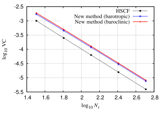
Figure 2: The values of VC versus the number of the grid points in the $r$ direction ($N_{r}$). Each line denotes rotating barotropic solutions by the new method (dashed line), rotating baroclinic solutions by the new method (solid line) and barotropic solutions by the HSCF scheme (dotted line).

Fig. 2 displays the convergence of the numerical results obtained via each numerical method. The lines denote the rotating baroclinic solutions using the new method (solid line), the rotating barotropic solutions using the new method (dashed line) and the rotating barotropic solutions using the HSCF scheme (dotted line). As seen in Fig. 2, the values of VC become smaller as the grid number in the $r$ direction increases. Both the barotropic (dotted line) and baroclinic (dashed lined) solutions obtained by the new method converged well. Although the values of the VC obtained by the new method are slightly larger than that obtained by HSCF scheme, they are sufficiently small and the solutions converged well (see Hachisu 1986a, b). Therefore, the numerical results by the new method are accurate and the numerical accuracy can be considered verified. In actual numerical calculations, which are tabulated and displayed in this paper, $N_{r}=512$ and $N_{\theta}=257$ are used.

3.1.2 Comparison with HSCF scheme

Next, the solutions obtained by the new numerical method were compared with those obtained by HSCF scheme to confirm the results. The baroclinic parameter was set as $\hat{\epsilon}=0$ to calculate the rotating barotropic equilibrium states by the new method. The same parameters ($N=1.5$ and $\hat{A}=0.9$) were used and seven models of rotating barotropic equilibrium states were calculated via both the new method and HSCF scheme. The seven solutions by each code are tabulated in Table 1. The left part of the table contains the numerical results obtained by the new method and the right one contains those obtained by HSCF scheme. The ’$*$’ in the table denotes the critical rotation model beyond which no rotating equilibrium state exists (Eriguchi & Mueller 1985; Hachisu 1986a). The isopycnic surfaces of the critical models are displayed in Fig. 3.

As seen in Table 1, the numerical results of the new method (left-hand side) are almost the same as those of the HSCF scheme (right-hand side). Although the values of $\hat{j}_{0}^{2}$ are slightly different the values of $\hat{K}_{0}$ and $T/|W|$ are almost identical. The critical rotation model was also obtained using the new method. Fig. 3 shows the isopycnic surfaces of the critical rotation models obtained by the new method (left-hand panel) and the HSCF scheme (right-hand panel). These isopycnic surfaces are almost identical as seen in the figures. The solutions of the critical rotation models have cusp structure at the equatorial surface (see right-hand panel). The cusp structure is calculated correctly by the new method (left-hand panel). Thus, the new method can calculate rapidly rotating barotropic stars correctly and accurately. The reliability of the new method is thus confirmed by this comparison with HSCF scheme.

Table 1: Physical quantities obtained by applying the new numerical method (left-hand) and the HSCF scheme (right-hand). The same parameters in both codes were used in both codes ($N=1.5$, $\hat{A}=0.9$). The solutions with ’*’ denote the critical rotation models beyond which no rotating equilibrium state exists.

$q$	$\hat{K}_{0}$	$\hat{j}_{0}^{2}$	$T/|W|$	VC
				New numerical method
0.900	2.691E$-$2	1.853E$-$2	2.232E$-$2	7.608E$-$6
0.801	2.368E$-$2	3.617E$-$2	4.698E$-$2	7.712E$-$6
0.699	2.020E$-$2	5.255E$-$2	7.492E$-$2	7.925E$-$6
0.600	1.662E$-$2	6.553E$-$2	1.048E$-$1	8.262E$-$6
0.500	1.272E$-$2	7.234E$-$2	1.359E$-$1	9.087E$-$6
0.400	7.737E$-$2	5.616E$-$2	1.351E$-$1	1.460E$-$5
0.395*	7.126E$-$2	5.107E$-$2	1.241E$-$1	1.658E$-$5

$q$	$\hat{K}_{0}$	$\hat{j}_{0}^{2}$	$T/|W|$	VC
				HSCF
0.900	2.691E$-$2	1.835E$-$2	2.210E$-$2	3.929E$-$6
0.801	2.368E$-$2	3.595E$-$2	4.668E$-$2	4.230E$-$6
0.699	2.021E$-$2	5.233E$-$2	7.458E$-$2	4.646E$-$6
0.600	1.661E$-$2	6.543E$-$2	1.047E$-$1	5.234E$-$6
0.500	1.271E$-$2	7.225E$-$2	1.357E$-$1	6.269E$-$6
0.400	7.702E$-$3	5.589E$-$2	1.345E$-$1	1.030E$-$5
0.395*	7.109E$-$3	5.093E$-$2	1.238E$-$1	1.140E$-$5

Figure 3: The isopycnic surfaces of the critical rotation models ($q=0.395$) calculated by the new method (left-hand panel) and the HSCF scheme (right-hand panel). The outermost curves denote the stellar surfaces. The difference between the two adjacent contours is $1/10$ of the maximum value of $\hat{\rho}$.

3.2 Rapidly rotating baroclinic equilibrium states

Finally, the rapidly rotating baroclinic equilibrium states were calculated using the new method. Two types of rotating baroclinic models were developed: a spherical isentropic surfaces model and an oblate isentropic surfaces model. The solution sequences of these two models were calculated systematically and the critical rotation solutions of these models were obtained via the new method. The Bjerknes–Rosseland rules, which must be satisfied by rotating baroclinic stars (c.f. Tassoul 1978), were checked, and all of the solutions were found to them.

3.2.1 Spherical isentropic surfaces model ($\hat{a}_{0}=\hat{b}_{0}$)

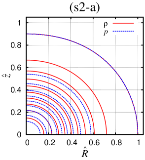
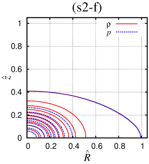
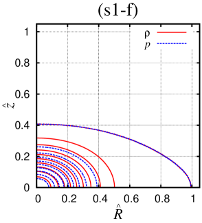
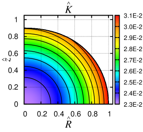
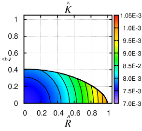
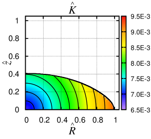
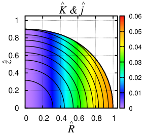
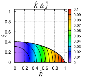
Figure 4: Distributions of the physical quantities. The three columns of figures display the distributions of solution (s2-a) (left-hand panels), solution (s2-f) (central panels) and solution (s1-f) (right-hand panels). From top to bottom, the four rows of figures correspond to the isopycnic surfaces (solid curves) and isobaric surfaces (dashed curves) (first row), the angular velocity isosurfaces (second row), the $\hat{K}$ isosurfaces (contours) and the value of $\hat{K}$ (colour maps) (third row) and the $\hat{K}$ isosurfaces (contours) and the value of the dimensionless specific angular momentum $\hat{j}$ (fourth row). The difference between the two adjacent contours is 1/10 of the difference between the maximum value and the minimum value.

Table 2: Physical quantities for the sequences with the spherical isentropic surfaces. The solutions with ’*’ denote the critical rotation models.

	$q$	$\hat{\epsilon}$	$\hat{a}_{0}$	$\hat{b}_{0}$	$m$	$\hat{K}_{0}$	$\hat{j}_{0}^{2}$	$T/|W|$	$\Pi/|W|$	VC
(s2-a)	0.900	0.35	1.0	1.0	2.0	2.300E$-$2	1.390E$-$2	1.910E$-2$	3.206E$-1$	8.447E$-6$
(s2-b)	0.801	0.35	1.0	1.0	2.0	1.980E$-$2	2.611E$-$2	3.940E$-2$	3.071E$-1$	8.817E$-6$
(s2-c)	0.699	0.35	1.0	1.0	2.0	1.776E$-$2	4.136E$-$2	6.579E$-2$	2.895E$-1$	8.816E$-6$
(s2-d)	0.599	0.35	1.0	1.0	2.0	1.472E$-$2	5.274E$-$2	9.342E$-2$	2.711E$-1$	9.285E$-6$
(s2-e)	0.500	0.35	1.0	1.0	2.0	1.133E$-$2	5.887E$-$2	1.212E$-2$	2.526E$-1$	1.046E$-5$
(s2-f)	0.408*	0.35	1.0	1.0	2.0	7.462E$-$3	5.009E$-$2	1.238E$-2$	2.508E$-1$	1.559E$-5$
(s1-a)	0.900	0.35	1.0	1.0	1.0	2.133E$-$2	1.369E$-$2	1.967E$-2$	3.202E$-1$	8.354E$-6$
(s1-b)	0.801	0.35	1.0	1.0	1.0	1.899E$-$2	2.718E$-$2	4.174E$-2$	3.055E$-1$	8.508E$-6$
(s1-c)	0.699	0.35	1.0	1.0	1.0	1.639E$-$2	4.009E$-$2	6.706E$-2$	2.886E$-1$	8.757E$-6$
(s1-d)	0.599	0.35	1.0	1.0	1.0	1.359E$-$2	5.062E$-$2	9.452E$-2$	2.703E$-1$	9.239E$-6$
(s1-e)	0.500	0.35	1.0	1.0	1.0	1.047E$-$2	5.601E$-$2	1.219E$-1$	2.520E$-1$	1.047E$-5$
(s1-f)	0.406*	0.35	1.0	1.0	1.0	6.833E$-$3	4.662E$-$2	1.225E$-1$	2.517E$-1$	1.607E$-5$

First, the rotating baroclinic stars with spherical isentropic surfaces were calculated as one of the simplest baroclinic models. The parameters of the equation of the state were fixed as $\hat{a}_{0}=\hat{b}_{0}=1.0$ to make a spherical isentropic surfaces. Two solution sequences (solutions (s1-) and (s2-)) with different $m$ were calculated by changing the value of $q$, and ten solutions (solutions (s1-a)–(s1-e) and (s2-a)–(s2-e)) and two baroclinic critical rotation solutions (solutions (s1-f) and (s2-f)) were obtained. The physical quantities of the numerical results are tabulated in Table 2. The solutions with ’*’ in Table 2 denote the critical rotation models. The structures of the solutions and distributions of the physical quantities are displayed in Fig. 4 with solution (s2-a) in the left-hand column, (s2-f) in the central column and (s1-f) in the right-hand column. From top to bottom, the four rows in Fig. 4 correspond to the isopycnic surfaces (solid curves) and isobaric surfaces (dashed curves) in the first row, the angular velocity isosurfaces in the second row, the $\hat{K}$ isosurfaces (contours) and the value of $\hat{K}$ (colour maps) in the third row and the $\hat{K}$ isosurfaces (contours) and the value of the dimensionless specific angular momentum $\hat{j}$ in the fourth row. The isopycnic surfaces and isopycnic surfaces of solution (s2-e) are also displayed in the left-hand panel of Fig. 1 to check the baroclinicity easily. Note that Fig. 1 shows the arbitrary seven isosurfaces and does not indicate the distributions of density and pressure.

As seen in the isobaric surfaces (solid curves) and the isopycnic surfaces in the left-hand panel of Fig. 1, the isobaric surfaces are always more oblate than the isopycnic surfaces. This tendency is also found in the first row in Fig. 4 (particularly solution s2-f). This baroclinicity comes from the entropy distributions inside the star. The third row shows the $\hat{K}$ isosurfaces (contours) and the values of $\hat{K}$ (colour maps). The $\hat{K}$ isosurfaces are spherical due to the functional form of equation (19). If we assume that the baroclinic ideal gas stars, these solutions have spherical isentropic surfaces because the specific entropy $s$ is proportional to $\hat{K}$ and the $\hat{K}$ isosurfaces denote the isentropic surfaces. The distributions of $\hat{K}$ in Fig. 4 indicate that the specific entropy increases outward and the equatorial specific entropy is higher than the polar specific entropy. Therefore, the surface temperature is colder at the poles than at the equator.

The second row shows the angular velocity ($\hat{\Omega}$) distributions. The equatorial angular velocity decreases outward because the profile of the angular velocity on the equatorial plane is fixed as equation (19). On the other hand, the angular velocity on the rotational axis increases from the centre to the surface ($\partial\hat{\Omega}/\partial\hat{z}>0$). Moreover, the values of $\partial\hat{\Omega}/\partial\hat{z}$ are always positive inside the star. The angular velocity distribution of a barotropic star is always purely cylindrical (Fig. 3), but baroclinicity causes the angular velocity distribution of a baroclinic star to not be cylindrical. The distribution is determined by the inclination angle of the isobaric and the isopycnic surfaces of the rotating star (equation 10). According to the Bjerknes–Rosseland rules, the value of $\partial\Omega/\partial z$ is always positive if the isobaric surfaces are more oblate than the isopycnic surfaces and the surface temperature is colder at the poles than at the equator (Tassoul 1978). All of these rotating baroclinic stars satisfy this rule correctly. The fourth row shows the $\hat{K}$ isosurfaces (contours) and the specific angular momentum $\hat{j}=(r\sin\theta)^{2}\Omega$ distributions (colour map). As seen in these panels, the specific angular momentum on each $\hat{K}$ isosurface ($s$ = constant surface) increases as we move from poles to the equator.

The axis ratios $q$ of both critical models are slightly larger than that of the rotating barotropic model (Table 1). The energy ratios $T/|W|$ of the critical rotating baroclinic stars are slightly smaller than that of barotropic one. The central and right-hand panels in Fig. 4 shows the critical rotation model with $m=2$ (central panels) and $m=1$ (right-hand panels). Although the isentropic surfaces of $m=1$ (s1-f) are more concentrated than those of $m=2$ (s2-f), the angular velocity distributions are similar. The parameter $m$ does change the distributions of the angular velocity very much. Therefore, the shape of the isentropic surfaces is more important for determining the distribution of the angular velocity.

Summarizing the above, the rotating baroclinic stars have spherical isentropic surfaces and the isobaric surfaces are more oblate than the isopycnic surfaces due to the entropy distribution. Such baroclinicity changes the angular velocity distributions and the value of $\partial\Omega/\partial z$ is always positive inside the star. This condition itself is one of the Bjerknes–Rosseland rule itself (Tassoul 1978). Therefore, all of these rotating baroclinic stars satisfy the Bjerknes–Rosseland rules.

3.2.2 Oblate isentropic surfaces models ($\hat{a}_{0}>\hat{b}_{0}$)

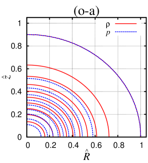
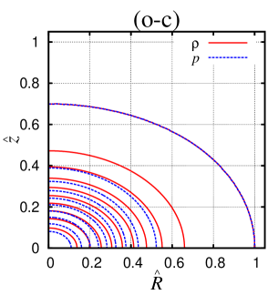
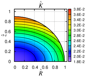
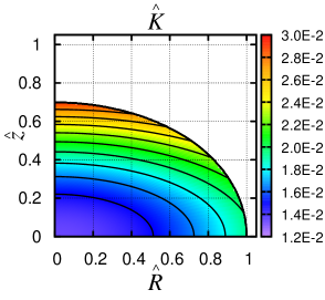
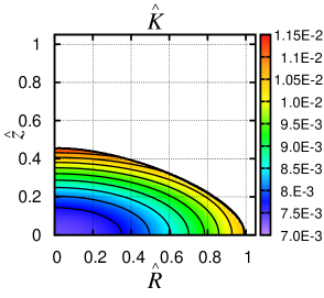
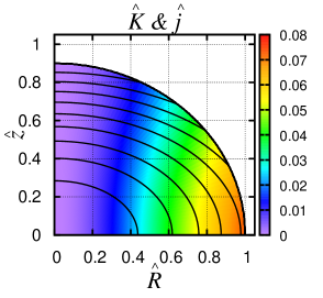
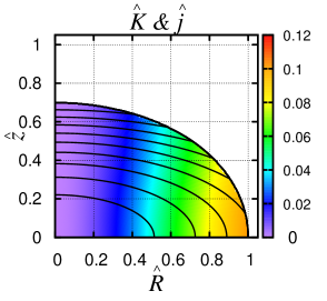
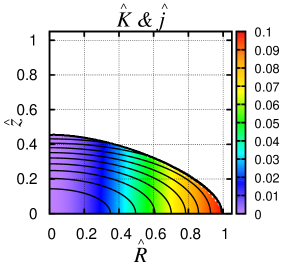
Figure 5: As per Fig. 4. The three columns of figures display the distributions of solution (o-c) (left-hand panels), solution (o-c) and solution of a critical rotation model (o-f), respectively.

Table 3: Physical quantities for the sequence with the oblate isentropic surfaces. The solution with ’*’ denotes the critical rotation model.

	$q$	$\hat{\epsilon}$	$\hat{a}_{0}$	$\hat{b}_{0}$	$m$	$\hat{K}_{0}$	$\hat{j}_{0}^{2}$	$T/|W|$	$\Pi/|W|$	VC
(o-a)	0.900	0.45	1.0	0.65	2.0	1.965E$-$2	2.557E$-$2	3.404E$-2$	3.106E$-1$	8.861E$-6$
(o-b)	0.801	0.45	1.0	0.50	2.0	1.609E$-$2	4.343E$-$2	6.365E$-2$	2.909E$-1$	9.212E$-6$
(o-c)	0.699	0.45	1.0	0.43	2.0	1.336E$-$2	5.253E$-$2	8.812E$-2$	2.746E$-1$	9.698E$-6$
(o-d)	0.599	0.45	1.0	0.41	2.0	1.118E$-$2	5.613E$-$2	1.076E$-1$	2.616E$-1$	1.051E$-6$
(o-e)	0.500	0.45	1.0	0.40	2.0	8.619E$-$3	5.366E$-$2	1.202E$-1$	2.532E$-1$	1.295E$-6$
(o-f)	0.455*	0.45	1.0	0.40	2.0	7.324E$-$3	4.860E$-$2	1.154E$-2$	2.563E$-1$	1.573E$-6$

Next, a rotating baroclinic star was calculated with oblate isentropic surfaces. The parameters of the equation of the state were fixed as $\hat{a}_{0}>\hat{b}_{0}$ in order to obtain the oblate isentropic surfaces inside the star. A solution sequence with $m=2$ was calculated by changing the value of $q$, and five solutions (solutions (o-a)–(o-e)) and a critical rotation solution (solution (o-f)) were obtained in the case of the oblate isentropic models. The numerical results are tabulated in table 3. The structures of the solutions and distributions of the physical quantities are displayed in Fig. 5. Solution (o-a) (left-hand column), (o-c) (central column) and (o-f) (right-hand column) are displayed in Fig. 5. The panels in Fig. 5 are presented similarly to Fig. 4. The arbitrary isopycnic surfaces and isopycnic surfaces of solution (o-a) are also displayed the right-hand panel of 1 to check the baroclinicity easily.

As seen in the isobaric surfaces (solid curve) and the isopycnic surfaces (dashed curves) in the right-hand panel of Fig. 1 the isopycnic surfaces are always more oblate than the isobaric surfaces. This tendency is also found in the first row in Fig. 5 (particularly solution (o-c)). This is the opposite situation to the spherical isentropic models seen in the previous subsection because the entropy distributions near the stellar surfaces are different from each other. The third row shows the $\hat{K}$ isosurfaces (contours) and the values of $\hat{K}$ (colour maps). The specific entropy in these models also increases outward, but the equatorial specific entropy is lower than the polar specific entropy. These entropy distributions mean that the surface temperature is hotter at the poles than at the equator. This distribution of the specific entropy is opposite to that of the spherical isentropic model. The distribution of the angular velocity is also opposite to that of the spherical isentropic model. The second row in Fig. 5 shows the angular velocity distributions. The values of $\partial\hat{\Omega}/\partial\hat{z}$ are always negative because of the entropy distributions. This tendency is also in contrast to the spherical isentropic model. According to the Bjerknes–Rosseland rules, the value of $\partial\Omega/\partial z$ is always negative if the isopycnic surfaces are more oblate than the isobaric surfaces and the surface temperature is hotter at the poles than at the equator (Tassoul 1978). All of these rotating baroclinic stars also satisfy the rules. The shapes of the angular velocity isosurfaces are interesting because they are clearly shellular-type (Fig. 5). In particular, those of solution (o-a) are almost perfectly shellular ones. Although their shapes are deformed by the rapid rotations, solutions (o-c) and (o-f) also have shellular-type rotation. The fourth row in Fig. 5 shows the $\hat{K}$ isosurfaces (contours) and the values of the specific angular momentum $\hat{j}$ (colour maps). The specific angular momentum on each isentropic surface also increases as we move from poles to the equator in these models.

Table 3 shows the solution sequence with the oblate isentropic surfaces. The critical rotation model (solution (o-f)) was obtained with the oblate isentropic model. The axis ratio of solution (o-f) is larger than that of the barotropic critical rotation and the energy ratio $T/|W|$ is smaller than that of the barotropic one. The axis ratio is also larger than those of solutions (s2-f) and (s1-f). The right-hand panels in Fig. 5 show the critical rotation model (solution (o-f)). The shellular-type rotation is realized even if the stellar rotation is as rapid as critical rotation.

Summarizing the above, these rotating baroclinic stars have oblate isentropic surfaces, and the isopycnic surfaces are more oblate than their isobaric surfaces due to the entropy distributions. Such baroclinicity makes angular velocity similar to that observed for shellular-type rotation, and the value of $\partial\Omega/\partial z$ always negative inside the star. This condition is also one of the Bjerknes–Rosseland rules (see e.g. Tassoul 1978). Therefore, all of these rotating baroclinic stars satisfy the Bjerknes–Rosseland rules.

4 Discussion and summary

4.1 Stability of rotating baroclinic stars

Stability analysis is an important problem to investigate for realistic rotating stars. Many types of instabilities are known to occur in rotating baroclinic stars, but we restrict ourselves to the consideration of instabilities arising from the stellar rotation in this paper. In particular, we focus on the dynamical instability due to the rotation that occurs because the time-scales of the shear instability arising from the differential rotation and the thermal instability (e.g. Goldreich & Schubert 1967) are much larger than that of the dynamical instability. We consider stability criteria derived from linear perturbation theory for rotating baroclinic stars.

The stability criteria of rotating stars are characterized by the specific angular momentum ($j=\Omega R^{2}$) distributions. According to the Høiland criterion, a baroclinic star in permanent rotation is dynamically stable with respect to axisymmetric motions if and only if the two following conditions are satisfied: (i) the specific entropy $s$ never decreases outward, and (ii) on each surface $s=$ constant (specific entropy constant), the angular momentum per unit mass (specific angular momentum $j$) increases from the poles to the equator (Tassoul 1978).

The thermal structures are totally independently and freely introduced to the mechanical structures in Newtonian gravity, because the thermal structures are obtained by assuming and adding thermal balance equations. If the ideal gas is adopted as one of the simplest equation of state, the specific entropy is determined and becomes proportional to $\hat{K}$. As seen earlier in this paper, the specific entropy never increases outward in all of the rotating baroclinic solutions in this paper. Therefore, all of the rotating baroclinic stars in this paper satisfy condition (i). The profiles of $j$ on $s=$ constant surfaces ($\hat{K}$ constant surfaces) are displayed in bottom panels in Figs. 4 and 5. As shown in these panels, the specific angular momentum on isentropic surface never decreases in both barotropic models. All of the rotating baroclinic stars in this paper also satisfy condition (ii). Therefore all of the rotating baroclinic stars satisfy the Høiland criterion. They are dynamically stable configurations against dynamical instability due to rotation. Further analysis of baroclinic rotating stars with realistic equations of state would be interest, but thermal balance (energy equation) must be solved to obtain the baroclinic stars with realistic equation of state. It is beyond the scope of the present paper. We will construct realistic rotating baroclinic models using this new numerical method and systematically analyse their stability in future works.

4.2 Shellular rotation

Many stellar evolution codes for rotating stars have adopted shellular rotation as one of their rotation models (e.g. Meynet & Maeder 1997; Talon et al. 1997; Heger et al. 2000; Mathis et al. 2004; Maeder & Meynet 2005; Potter et al. 2012a, b; Takahashi et al. 2014). The first shellular rotation model was formulated and derived by Zahn (1992) using a perturbative approach. When the turbulence is anisotropic with stronger matter transport in the horizontal directions than in the vertical, shellular rotation is realized (Zahn 1992). As a result, the horizontal-dependence of the angular velocity disappears and the angular velocity depends on only the distance from the centre of the star. This kind of shellular rotation was adopted as an initial rotation profile of core-collapse supernova simulations (e.g. Yamada & Sato 1994). However, nobody had successfully investigated self-consistent configurations of rapidly rotating stars with shellular rotation systematically because of the difficulty of obtaining rotating baroclinic stars.

Some previous works showed self-consistent rotating baroclinic stars with non-cylindrical rotations (Uryu & Eriguchi 1994; Uryu & Eriguchi 1995; Espinosa Lara & Rieutord 2007; Espinosa Lara & Rieutord 2013), but their rotation distributions were far from shellular. On the other hand, Roxburgh (2006) calculated rotating baroclinic stars by fixing the distribution of the shellular rotation, but neither calculated solutions systematically nor obtained critical rotation models. Kiuchi et al. (2010) investigated multi-layered configurations in differentially rotational equilibrium. While they did obtain rapidly rotating solutions systematically, they calculated rotating barotropic stars only.

In contrast, this paper has investigated rapidly rotating baroclinic stars systematically as in Section 3.3. The oblate isentropic surfaces models were found to have shellular-type angular velocity distributions. The equatorial surface temperature of the rotating baroclinic star is hotter than the polar temperature. These kinds of entropy and temperature distributions generate shellular-type rotation. Shellular-type rotation is realized even if the star has very rapid rotation. Solution (o-f) is a critical rotation model and its distribution of the angular velocity is shellular-type (Fig.5). These are the first self-consistent and systematic solutions of the rapidly baroclinic stars with shellular-type rotations. These shellular-type rotating stars are dynamically stable as they all satisfy the Høiland criterion as seen in Section 4.1. This kind of shellular-type rotation would be realized in many rapidly rotating stars.

4.3 Summary

A versatile numerical method for obtaining structures of rapidly rotating baroclinic stars was investigated. The novel numerical method was based on the self-consistent field scheme and the solution was obtained iteratively. Both rotating barotropic and baroclinic stars were calculated systematically by using the new method. The accuracy of the new method was verified by checking the convergence of numerical results. The relative values of the virial relation were small and converged well. Further, the solutions from the new method and those obtained by the HSCF scheme, a well-established numerical scheme, were compared, and the solutions were very similar.

Two types of rotating baroclinic stars — spherical isentropic surfaces models and oblate isentropic surfaces models — were investigated by fixing functional forms of a simple baroclinic equation of state. Solution sequences of both models were calculated systematically and the critical rotation models were also obtained. All of the rotating baroclinic stars satisfy the Bjerknes–Rosseland condition. In the spherical isentropic surfaces model, the isobaric surfaces are more oblate than the isopycnic surfaces and the values of $\partial\Omega/\partial z$ are always positive throughout the star. In the oblate isentropic surfaces model, on the other hand, the isopycnic surfaces are more oblate than the isobaric surfaces and the values of $\partial\Omega/\partial z$ are always negative throughout the star. The baroclinic star with shellular-type rotation was found to be realized when isentropic surfaces are oblate and the equatorial surface temperature of the rotating baroclinic star is hotter than the polar temperature if it is assumed that the star is the ideal gas star. The shellular-type rotation is realized even if the rotation is as rapid as possible. These are the first self-consistent and systematic solutions of the rapidly rotating baroclinic stars with shellular-type rotations.

The Høiland criterion of the rotating baroclinic stars was checked, with all solutions in this paper satisfying the criterion. Therefore, these rotating baroclinic star are stable against the dynamical instability due to the rotation. Realistic rotating baroclinic stars with a realistic equation of state are needed to investigate the evolution of the rapidly realistic rotating stars. Further works may extend the numerical method and calculate realistic rotating baroclinic stars.

Appendix A Details of numerical scheme

The numerical scheme of the new method is described in detail. The numerical scheme is based on a self-consistent field iteration scheme (Ostriker & Mark 1968; Hachisu 1986a, b). The gravitational field and all physical quantities are determined iteratively. A numerical domain of the computation is defined as $0\leq\hat{r}\leq 2$ in the radial direction and $0\leq\theta\leq\pi/2$ in the angular direction. The numerical domains are discretized into mesh points with equal intervals $\Delta\hat{r}$ and $\Delta\theta$, respectively as

$$\hat{r}_{i}=i\times\Delta\hat{r},\hskip 10.0pt\Delta\hat{r}=\frac{1}{N_{r}},\hskip 10.0pti=0,1,2,3,\cdots,$$ (27)

$$\theta_{j}=(j-1)\times\Delta\theta,\hskip 10.0pt\Delta\theta=\frac{\pi/2}{N_{\theta}-1},\hskip 10.0ptj=1,2,3,\cdots.$$ (28)

Physical variables are defined at the cross point of two mesh lines, i.e.,

$$\hat{\rho}_{i,j}=\hat{\rho}(\hat{r}_{i},\theta_{j}).$$ (29)

Before the first iteration cycle, a one-dimensional spherical non-rotating barotropic star is used as the initial guess for two-dimensional rotating star. The value of $\hat{K}_{0}$ is determined to make the radius of the 1D spherical star unity. The values of $\hat{K}_{0}$ and the 1D star are used for the iteration.

We start the iteration cycle after the initial guesses are obtained. First, we calculate the gravitational potential $\hat{\phi}$ from the initial guess of $\hat{\rho}$ as

$$\hat{\phi}=-\sum_{\ell=0}^{\ell_{\max}}P_{2\ell}(\cos\theta)\int_{0}^{\infty}\hat{r}^{\prime 2}f_{2\ell}(\hat{r},\hat{r}^{\prime})d\hat{r}^{\prime}$$

$$\times\int_{0}^{\pi/2}P_{2\ell}(\cos\theta^{\prime})\sin\theta^{\prime}d\theta^{\prime}\hat{\rho}(\hat{r}^{\prime},\theta^{\prime}),$$ (30)

where $P_{2\ell}$ is a Lgendre polynomial and $f_{2\ell}(\hat{r},\hat{r}^{\prime})$ is a function defined by

$$f_{2\ell}(\hat{r},\hat{r}^{\prime})=\left\{\begin{array}[]{cc}\hat{r}^{\prime 2\ell}/\hat{r}^{2\ell+1}&(\hat{r}>\hat{r}^{\prime})\\ \hat{r}^{2\ell}/\hat{r}^{\prime 2\ell+1}&(\hat{r}<\hat{r}^{\prime}).\end{array}\right.$$ (33)

Simpson’s scheme is used to calculate the integrals numerically. $\ell_{\max}$ is fixed as $2\ell_{\max}=40$ in all numerical calculations in this paper.

Next, we calculate the values of $\hat{j}_{0}$ and $\hat{K}_{0}$. These values are determined in order to make the equatorial radius unity and the axis ratio $q$. First, we calculate the value of $\hat{K}_{0}$ by solving the dimensionless form of the $r$ component of the Euler equation (equation 5) with the equation of state (equation 19) on the rotational axis. The equations on the rotational axis are respectively discretized as follow:

$$\frac{\hat{p}_{i,1}-\hat{p}_{i-1,1}}{\Delta\hat{r}}=\frac{(\hat{\rho}_{i,1}+\hat{\rho}_{i-1,1})}{2}\frac{(\hat{\phi}_{i,1}-\hat{\phi}_{i-1,1})}{\Delta\hat{r}},$$ (34)

$$\hat{p}_{i,1}=\hat{K}_{0}\left\{1+\epsilon\left(\frac{1}{\hat{b}_{0}^{2}}\right)\hat{r}_{i,1}^{m}\right\}\left(\hat{\rho}_{i,1}\right)^{1+\frac{1}{N}}.$$ (35)

A central difference was adopted in this numerical scheme. We start the integration at the centre of the star ($\hat{r}=0$). Since we have defined the dimensionless form of the central density in equations (18) and (20), the values of $\hat{\rho}_{1,1}$ and $\hat{p}_{1,1}$ are obtained by solving the discretized equations using the values of $\hat{\rho}_{c}$ and $\hat{p}_{c}$. Then, the values of $\hat{\rho}_{2,1}$ and $\hat{p}_{2,1}$ are determined using the values of $\hat{\rho}_{1,1}$ and $\hat{p}_{1,1}$. The integration is continued until the density $\hat{\rho}_{i,1}$ becomes zero ($\hat{\rho}_{i,1}=0)$, and we obtain the value of the polar radius $\hat{r}_{\rm pol.}$ after the integration. If the value of $\hat{r}_{\rm pol.}$ is different from the value of $q$, we change the value of $\hat{K}_{0}$ and restart the integration using a shooting-type method (Press et al. 1992) until we obtain the value of $\hat{K}_{0}$ that makes the polar radius ($\hat{r}_{\rm pol.}$) $q$. Next, we calculate the value of $\hat{j}_{0}$ by solving the dimensionless form of the $r$ component of the Euler equation (equation 5) and the equation of state (equation 19) on the equatorial axis. The equations on the equatorial plane are discretized as follows:

$$\frac{\hat{p}_{i,N_{\theta}}-\hat{p}_{i-1,N_{\theta}}}{\Delta\hat{r}}=\frac{(\hat{\rho}_{i,N_{\theta}}+\hat{\rho}_{i-1,N_{\theta}})}{2}\frac{(\hat{\phi}_{i,N_{\theta}}-\hat{\phi}_{i-1,N_{\theta}})}{\Delta\hat{r}}$$

$$+\frac{(\hat{r}_{i}+\hat{r}_{i-1})}{2}\frac{(\hat{\rho}_{i,N_{\theta}}+\hat{\rho}_{i-1,N_{\theta}})}{2}\frac{(\hat{\Omega}^{2}_{i,N_{\theta}}+\hat{\Omega}^{2}_{i-1,N_{\theta}})}{2},$$ (36)

$$\hat{p}_{i,N_{\theta}}=\hat{K}_{0}\left\{1+\epsilon\left(\frac{1}{\hat{a}_{0}^{2}}\right)\hat{r}_{i,N_{\theta}}^{m}\right\}\left(\hat{\rho}_{i,N_{\theta}}\right)^{1+\frac{1}{N}}.$$ (37)

The value of $\hat{j}_{0}$ is determined in the same manner to make the equatorial radius unity.

Figure 6: Schematic images of the numerical scheme for $\hat{\Omega}$ (left-hand panel) and $\hat{\rho}$, $\hat{p}$ (right-hand panel). The thick curve denotes the stellar surface. $(i,j)$ denotes the mesh point and each number refers to the sequence of the integration. We start the integration of equations at point 1.

After the new values of $\hat{K}_{0}$ and $\hat{j}_{0}$ have been obtained, the distribution of the angular velocity can be calculated using the dimensionless forms of equations (10) and (21). Four neighbouring mesh points [$(i-1,j)$, $(i,j)$, $(i-1,j+1)$ and $(i,j+1)$] are used to solve equation (10) in this numerical scheme. The equation is discretized at the centre of the four mesh points (left-hand panel of Fig. 6). The explicit form of the discretized equation is

$$\hat{r}_{m}^{2}\sin\theta_{m}\cos\theta_{m}\frac{(\hat{\Omega}^{2}_{i,j}+\hat{\Omega}^{2}_{i,j+1})-(\hat{\Omega}^{2}_{i-1,j}+\hat{\Omega}^{2}_{i-1,j+1})}{2\Delta\hat{r}}$$ (38)

$$-\hat{r}_{m}\sin^{2}\theta_{m}\frac{(\hat{\Omega}^{2}_{i,j+1}+\hat{\Omega}^{2}_{i-1,j+1})-(\hat{\Omega}^{2}_{i,j}+\hat{\Omega}^{2}_{i-1,j})}{2\Delta\theta}$$

$$= \frac{1}{\hat{\rho}_{m}^{2}}\Bigg{[}\left\{\frac{(\hat{\rho}_{i,j+1}+\hat{\rho}_{i-1,j+1})-(\hat{\rho}_{i,j}+\hat{\rho}_{i-1,j})}{2\Delta\theta}\right\}$$

$$\times\left\{\frac{(\hat{p}_{i,j+1}+\hat{p}_{i,j})-(\hat{p}_{i-1,j+1}+\hat{p}_{i-1,j})}{2\Delta\hat{r}}\right\}$$

$$- \left\{\frac{(\hat{p}_{i,j+1}+\hat{p}_{i-1,j+1})-(\hat{p}_{i,j}+\hat{p}_{i-1,j})}{2\Delta\theta}\right\}$$

$$\times\left\{\frac{(\hat{\rho}_{i,j+1}+\hat{\rho}_{i,j})-(\hat{\rho}_{i-1,j+1}+\hat{\rho}_{i-1,j})}{2\Delta\hat{r}}\right\}\Bigg{]},$$

where $\hat{r}_{m}$, $\theta_{m}$ and $\hat{\rho}_{m}$ are

$$\hat{r}_{m}=\frac{1}{2}\left(\hat{r}_{i}+\hat{r}_{i-1}\right),$$ (39)

$$\theta_{m}=\frac{1}{2}\left(\theta_{j+1}+\theta_{j}\right),$$ (40)

$$\hat{\rho}_{m}=\frac{1}{4}\left(\hat{\rho}_{i-1,j}+\hat{\rho}_{i,j}+\hat{\rho}_{i-1,j+1}+\hat{\rho}_{i,j+1}\right).$$ (41)

In this scheme, the value of $\hat{\Omega}_{i,j}^{2}$ is calculated by using the values of $\hat{\Omega}_{i-1,j}^{2}$, $\hat{\Omega}^{2}_{i-1,j+1}$ and $\hat{\Omega}^{2}_{i,j+1}$. Fig. 6 displays schematic images of this scheme. For simplicity, Fig. 6 has assumed mesh numbers $N_{r}=3$ and $N_{\theta}=3$. We start the integration at point 1 in the left-hand panel of Fig. 6. First, the boundary condition on the equatorial plane is set. The values of $\hat{\Omega}^{2}_{0}$, $\hat{\Omega}^{2}_{1,3}$, $\hat{\Omega}^{2}_{2,3}$ and $\hat{\Omega}^{2}_{3,3}$ are fixed during the iterations. At point 1 in the left-hand panel of Fig. 6, we obtain the value of $\Omega^{2}_{1,2}$ from equation (38) by using the values of $\hat{\Omega}^{2}_{0}$ and $\hat{\Omega}^{2}_{1,3}$ because $\hat{\Omega}^{2}_{0,3}=\hat{\Omega}^{2}_{0,2}=\hat{\Omega}^{2}_{0}$ at point 1. Then, we move to point 2 and calculate $\hat{\Omega}^{2}_{2,2}$ by using the values of $\hat{\Omega}^{2}_{1,3}$, $\hat{\Omega}^{2}_{2,3}$ and $\hat{\Omega}^{2}_{1,2}$, and solving the equation.

Finally, we calculate the distributions of $\hat{\rho}$ and $\hat{p}$ from equations (5) and (19) by using the distributions of $\hat{\phi}$ and $\hat{\Omega}^{2}$. The two mesh points ($(i,j)$ and $(i-1,j)$) are used in this calculation. The equation is discretized as

$$\frac{\hat{p}_{i,j}-\hat{p}_{i-1,j}}{\Delta\hat{r}}=\frac{(\hat{\rho}_{i,j}+\hat{\rho}_{i-1,j})}{2}\frac{(\hat{\phi}_{i,j}-\hat{\phi}_{i-1,j})}{\Delta\hat{r}}$$

$$+\frac{(\hat{r}_{i}+\hat{r}_{i-1})}{2}\sin\theta^{2}_{j}\frac{(\hat{\rho}_{i,j}+\hat{\rho}_{i-1,j})}{2}\frac{(\hat{\Omega}_{i,j}^{2}+\hat{\Omega}^{2}_{i-1,j})}{2}$$ (42)

and the equation of state is given as

$$\hat{p}_{i,j}=\hat{K}_{0}\left\{1+\epsilon\left(\frac{\sin\theta_{j}}{\hat{a}_{0}^{2}}+\frac{\cos\theta_{j}}{\hat{b}_{0}^{2}}\right)\hat{r}_{i}^{m}\right\}\left(\hat{\rho}_{i,j}\right)^{1+\frac{1}{N}}.$$ (43)

We start the integration at point 1 in the right-hand panel of Fig. 6. Since the central density and the central pressure have been fixed as $\hat{\rho}_{0}=\hat{\rho}_{c}=1$ and $\hat{p}_{0}=\hat{p}_{c}$ by equations (20) and (43), we calculate $\hat{\rho}_{1,3}$ and $\hat{p}_{1,3}$ by equation (42). Next, we move to point 2 and obtain $\hat{\rho}_{2,3}$ and $\hat{p}_{2,3}$ by using the values of $\hat{\rho}_{1,3}$ and $\hat{p}_{1,3}$ and equations (42) and (43). We can obtain the values of $\hat{\rho}_{i,j}$ and $\hat{p}_{i,j}$ by using the values of $\hat{\rho}_{i-1,j}$ and $\hat{p}_{i-1,j}$ . If the value of $\hat{\rho}_{i,j}$ or $\hat{p}_{i,j}$ is zero, we search the location of the stellar surface $\hat{r}_{s}(\theta)$, where $\hat{r}_{s}(\theta)$ denotes the dimensionless radius in each $\theta$ direction. After calculating the location of the surface, we move to point 4 and continue the integration. After the integration on the rotational axis (point 6 in the panel), we have obtained new distributions of $\hat{\rho}$ and $\hat{p}$ and one iteration cycle is finished.

In summary, the numerical iteration cycle of this method is as follows.

1. Set the parameters ($N$, $q$) and fix the functional forms of $\hat{\Omega}^{2}$ on the equatorial plane and the equation of state.

2. Make an initial guess for the two-dimensional rotating baroclinic star. Calculate a one-dimensional spherical barotropic star for initial guesses of the iteration.

3. Calculate the gravitational potential $\hat{\phi}$ by using the distribution of $\hat{\rho}$.

4. Calculate the values of $\hat{K}_{0}$ and $\hat{j}_{0}$ via a shooting-type method in order to make the equatorial radius unity and the axis ratio $q$.

5. Calculate the angular velocity $\hat{\Omega}$ by using the distribution of $\hat{\phi}$ obtained in (iii).

6. Solve the $r$-component of the Euler equation with the equation of state and obtain the new distributions of density $\hat{\rho}$ and pressure $\hat{p}$ by using the distributions of $\hat{\phi}$ obtained in (iii) and $\hat{\Omega}$ obtained in (v).

7. Check the convergence of the system. Compare the new and old density distributions. If the relative differences between the new distributions and the old distributions are sufficiently small (e.g. smaller than $\sim 10^{-4}$), the system is considered to converge well and the iteration cycle finishes as the rotating baroclinic star has been obtained in equilibrium. If the system does not converge, return to (iii) and start a new iteration cycle until the system converge.

References

- Bonazzola et al. (1998) Bonazzola S., Gourgoulhon E., Marck J.-A., 1998, Phys. Rev. D, 58, 104020
- Che et al. (2011) Che X., Monnier J. D., Zhao M., Pedretti E., Thureau N., Mérand A., ten Brummelaar T., McAlister H., Ridgway S. T., Turner N., Sturmann J., Sturmann L., 2011, ApJ, 732, 68
- Clement (1969) Clement M. J., 1969, ApJ, 156, 1051
- Dufton et al. (2013) Dufton P. L., Langer N., Dunstall P. R., Evans C. J., Brott I., de Mink S. E., Howarth I. D., Kennedy M., McEvoy C., Potter A. T., Ramírez-Agudelo O. H., Sana H., Simón-Díaz S., Taylor W., Vink J. S., 2013, A&A, 550, A109
- Ekström et al. (2008) Ekström S., Meynet G., Maeder A., Barblan F., 2008, A&A, 478, 467
- Eriguchi & Mueller (1985) Eriguchi Y., Mueller E., 1985, A&A, 146, 260
- Eriguchi & Mueller (1991) —, 1991, A&A, 248, 435
- Espinosa Lara & Rieutord (2007) Espinosa Lara F., Rieutord M., 2007, A&A, 470, 1013
- Espinosa Lara & Rieutord (2013) —, 2013, A&A, 552, A35
- Faulkner et al. (1968) Faulkner J., Roxburgh I. W., Strittmatter P. A., 1968, ApJ, 151, 203
- Fujisawa (2015) Fujisawa K., 2015, MNRAS, 450, 4016
- Fujisawa & Eriguchi (2013) Fujisawa K., Eriguchi Y., 2013, MNRAS, 432, 1245
- Fujisawa et al. (2012) Fujisawa K., Yoshida S., Eriguchi Y., 2012, MNRAS, 422, 434
- Goldreich & Schubert (1967) Goldreich P., Schubert G., 1967, ApJ, 150, 571
- Hachisu (1986a) Hachisu I., 1986a, ApJS, 61, 479
- Hachisu (1986b) —, 1986b, ApJS, 62, 461
- Heger et al. (2000) Heger A., Langer N., Woosley S. E., 2000, ApJ, 528, 368
- Hunter et al. (2008) Hunter I., Lennon D. J., Dufton P. L., Trundle C., Simón-Díaz S., Smartt S. J., Ryans R. S. I., Evans C. J., 2008, A&A, 479, 541
- Jackson (1970) Jackson S., 1970, ApJ, 161, 579
- Jackson et al. (2005) Jackson S., MacGregor K. B., Skumanich A., 2005, ApJS, 156, 245
- Kippenhahn & Thomas (1970) Kippenhahn R., Thomas H.-C., 1970, in IAU Colloq. 4: Stellar Rotation, Slettebak A., ed., p. 20
- Kiuchi et al. (2010) Kiuchi K., Nagakura H., Yamada S., 2010, ApJ, 717, 666
- Langer (2012) Langer N., 2012, ARA&A, 50, 107
- Maeder (2009) Maeder A., 2009, Physics, Formation and Evolution of Rotating Stars
- Maeder & Meynet (2000) Maeder A., Meynet G., 2000, ARA&A, 38, 143
- Maeder & Meynet (2005) —, 2005, A&A, 440, 1041
- Mathis (2013) Mathis S., 2013, in Lecture Notes in Physics, Berlin Springer Verlag, Vol. 865, Lecture Notes in Physics, Berlin Springer Verlag, Goupil M., Belkacem K., Neiner C., Lignières F., Green J. J., eds., p. 23
- Mathis et al. (2004) Mathis S., Palacios A., Zahn J.-P., 2004, A&A, 425, 243
- Meynet & Maeder (1997) Meynet G., Maeder A., 1997, A&A, 321, 465
- Monaghan (1971) Monaghan J. J., 1971, MNRAS, 154, 47
- Ostriker & Mark (1968) Ostriker J. P., Mark J., 1968, ApJ, 151, 1075
- Papaloizou & Whelan (1973) Papaloizou J. C. B., Whelan J. A. J., 1973, MNRAS, 164, 1
- Potter et al. (2012a) Potter A. T., Tout C. A., Brott I., 2012a, MNRAS, 423, 1221
- Potter et al. (2012b) Potter A. T., Tout C. A., Eldridge J. J., 2012b, MNRAS, 419, 748
- Press et al. (1992) Press W. H., Teukolsky S. A., Vetterling W. T., Flannery B. P., 1992, Numerical recipes in FORTRAN. The art of scientific computing
- Ramírez-Agudelo et al. (2013) Ramírez-Agudelo O. H., Simón-Díaz S., Sana H., de Koter A., Sabín-Sanjulían C., de Mink S. E., Dufton P. L., Gräfener G., Evans C. J., Herrero A., Langer N., Lennon D. J., Maíz Apellániz J., Markova N., Najarro F., Puls J., Taylor W. D., Vink J. S., 2013, A&A, 560, A29
- Rieutord (1987) Rieutord M., 1987, Geophysical and Astrophysical Fluid Dynamics, 39, 163
- Roxburgh (2004) Roxburgh I. W., 2004, A&A, 428, 171
- Roxburgh (2006) —, 2006, A&A, 454, 883
- Roxburgh et al. (1965) Roxburgh I. W., Griffith J. S., Sweet P. A., 1965, ZAp, 61, 203
- Roxburgh & Strittmatter (1966) Roxburgh I. W., Strittmatter P. A., 1966, MNRAS, 133, 345
- Sackmann & Anand (1970) Sackmann I.-J., Anand S. P. S., 1970, ApJ, 162, 105
- Sharp et al. (1977) Sharp C. M., Smith R. C., Moss D. L., 1977, MNRAS, 179, 699
- Takahashi et al. (2014) Takahashi K., Umeda H., Yoshida T., 2014, ApJ, 794, 40
- Talon et al. (1997) Talon S., Zahn J.-P., Maeder A., Meynet G., 1997, A&A, 322, 209
- Tassoul (1978) Tassoul J.-L., 1978, Theory of rotating stars
- Tomimura & Eriguchi (2005) Tomimura Y., Eriguchi Y., 2005, MNRAS, 359, 1117
- Uryu & Eriguchi (1994) Uryu K., Eriguchi Y., 1994, MNRAS, 269, 24
- Uryu & Eriguchi (1995) —, 1995, MNRAS, 277, 1411
- von Zeipel (1924) von Zeipel H., 1924, MNRAS, 84, 665
- Yamada & Sato (1994) Yamada S., Sato K., 1994, ApJ, 434, 268
- Yasutake et al. (2015) Yasutake N., Fujisawa K., Yamada S., 2015, MNRAS, 446, L56
- Yoshida et al. (2012) Yoshida S., Kiuchi K., Shibata M., 2012, Phys. Rev. D, 86, 044012
- Zahn (1992) Zahn J.-P., 1992, A&A, 265, 115