Fifteen years of XMM-Newton and Chandra monitoring of Sgr A^⋆: Evidence for a recent increase in the bright flaring rate

Abstract

We present a study of the X-ray flaring activity of Sgr A^⋆ during all the 150 XMM-Newton and Chandra observations pointed at the Milky Way center over the last 15 years. This includes the latest XMM-Newton and Chandra campaigns devoted to monitoring the closest approach of the very red Br $\gamma$ emitting object called G2. The entire dataset analysed extends from September 1999 through November 2014. We employed a Bayesian block analysis to investigate any possible variations in the characteristics (frequency, energetics, peak intensity, duration) of the flaring events that Sgr A^⋆ has exhibited since their discovery in 2001. We observe that the total bright-or-very bright flare luminosity of Sgr A^⋆ increased between 2013-2014 by a factor of 2-3 ($\sim 3.5\sigma$ significance). We also observe an increase ($\sim 99.9$ % significance) from $0.27\pm 0.04$ to $2.5\pm 1.0$ day^-1 of the bright-or-very bright flaring rate of Sgr A^⋆, starting in late summer 2014, which happens to be about six months after G2’s peri-center passage. This might indicate that clustering is a general property of bright flares and that it is associated with a stationary noise process producing flares not uniformly distributed in time (similar to what is observed in other quiescent black holes). If so, the variation in flaring properties would be revealed only now because of the increased monitoring frequency. Alternatively, this may be the first sign of an excess accretion activity induced by the close passage of G2. More observations are necessary to distinguish between these two hypotheses.

1 Introduction

Sgr A^⋆, the radiative counterpart of the supermassive black hole (BH) at the center of the Milky Way radiates currently at a very low rate, about nine orders of magnitude lower than the Eddington luminosity for its estimated mass of M${}_{\rm BH}\sim 4.4\times 10^{6}$ M_⊙ (Ghez et al. 2008; Genzel et al. 2010). The first Chandra observations of Sgr A^⋆ determined the quiescent, absorption-corrected, 2–10 keV X-ray luminosity to be L${}_{\rm 2-10~{}keV}\sim 2\times 10^{33}$ erg s^-1 (Baganoff et al. 2003). This emission is constant in flux, spatially extended and possibly due to a radiatively inefficient accretion flow (Rees et al. 1982; Wang et al. 2013). On top of the very stable quiescent emission, high-amplitude X-ray flaring activity, with variations up to factors of a few hundred times the quiescent level is commonly observed (Baganoff et al. 2001; Goldwurm et al. 2003; Porquet et al. 2003; 2008; Nowak et al. 2012; Neilsen et al. 2013; Degenaar et al. 2013; Barrière et al. 2014; Haggard et al. 2015). The most sensitive instruments (e.g., Chandra) established that X-ray flares occur on average once per day and they last from several minutes up to a few hours, reaching peak luminosities of $\sim 5\times 10^{35}$ erg s^-1. In particular, all the observed flares to date have an absorbed power-law spectral shape (that will hereinafter be used as our baseline model) consistent with a spectral index of 2-2.2 (Porquet et al. 2008; Nowak et al. 2012; but see also Barrière et al. 2014). Soon after the discovery of the first X-ray flares, the infra-red (IR) counterpart of such events was revealed (Genzel et al. 2003; Ghez et al. 2004). Though every X-ray flare has an IR counterpart, IR flares occur more frequently ($\sim 4$ times higher rate) than the X-ray flares. Moreover, the IR emission is continuously variable with no constant level of quiescent emission at low fluxes (Meyer et al. 2009).

The origin of Sgr A^⋆’s flares is still not completely understood. The accreting material mostly comes from parts of the stellar winds of the stars orbiting Sgr A^⋆ (Melia 1992; Coker & Melia 1997; Rockefeller et al. 2004; Cuadra et al. 2005; 2006; 2008). The sudden flares might be a product of magnetic reconnection, or stochastic acceleration or shocks (possibly associated with jets) at a few gravitational radii from Sgr A^⋆ (Markoff et al. 2001; Liu & Melia 2002; Liu et al. 2004; Yuan et al. 2003; 2004; 2009; Marrone et al. 2008; Dodds-Eden et al. 2009). Other mechanisms, for instance associated with the tidal disruption of asteroids, have also been proposed (Čadež et al. 2008; Kostić et al. 2009; Zubovas et al. 2012). To shed light on the radiative mechanism of the flares, several multi-wavelength campaigns have been performed (Eckart et al. 2004; 2006; 2008; 2009; 2012 Yusef-Zadeh et al. 2006; 2008; 2009; Hornstein et al. 2007; Marrone et al. 2008; Dodds-Eden et al. 2009; Trap et al. 2011). Sgr A^⋆’s spectral energy distribution, during flares, shows two peaks of emission, one at IR and the second at X-ray wavelengths. The IR peak is consistent with being produced by synchrotron emission (polarisation is observed in the submm and IR), while a variety of processes could produce the X-ray peak, including synchrotron and inverse Compton processes like synchrotron self-Compton and external Compton (see Genzel et al. 2010 for a review). Synchrotron emission, extending with a break from IR to the X-ray range, seems now the best process able to account for the X-ray data with reasonable physical parameters (Dodds-Eden et al. 2009, Trap et al. 2010, Barrière et al. 2014).

A detailed analysis of the X-ray flare distribution (taking advantage of the 3 Ms Chandra monitoring campaign performed in 2012) shows that weak flares are the most frequent, with an underlying power-law flare luminosity distribution $dN/dL$ of index $\Gamma\sim-1.9$ (Neilsen et al. 2013; 2015). In particular, flares with $L_{\rm 2-8~{}keV}>10^{34}$ erg s^-1 occur at a rate of $1.1^{+0.2}_{-0.1}$ per day, while luminous flares (with $L_{\rm 2-8~{}keV}>10^{35}$ erg s^-1) occur every $\sim 10$ days (Neilsen et al. 2013; 2015; Degenaar et al. 2013). The occurrence of flares appears to be randomly distributed and stationary. Based on the detection of a bright flare plus three weaker ones during a $\sim 230$ ks XMM-Newton monitoring of Sgr A^⋆, Bèlanger et al. (2005) and Porquet et al. (2008) argue that Sgr A^⋆’s flares might occur primarily in clusters. An even higher flaring rate was actually recorded during a $\sim 23$ ks Chandra observation (obsID: 13854) when 4 weak flares were detected (Neilsen et al. 2013; with an associated chance probability of about 3.5 %; Neilsen et al. 2015). However, no significant variation of the flaring rate has yet been established.

Recently, long Chandra, XMM-Newton and Swift X-ray observing campaigns have been performed to investigate any potential variation in Sgr A^⋆’s X-ray properties induced by the interaction between Sgr A^⋆ and the gas-and-dust-enshrouded G2 object (Gillessen et al. 2012; Witzel et al. 2014). We analyse here all the existing XMM-Newton and Chandra observations of Sgr A^⋆ to search for variations in the X-ray flaring rate. The Swift results are discussed elsewhere (Degenaar et al. 2015).

This paper is structured as follows. In § 2 we summarise the XMM-Newton and Chandra data reduction. In § 3 we present the XMM-Newton monitoring campaigns performed in 2013 and 2014. In § 4 we describe the application of the Bayesian block analysis to the 15 years of XMM-Newton and Chandra data and derive the parameters and fluence for each detected flare. We also present the flare fluence distribution. In § 5 we investigate possible variations to the flaring rate of Sgr A^⋆ and in § 6 the change in the total luminosity emitted in bright flares. Sections 7 and 8 present the discussion and conclusions.

2 Data reduction

2.1 XMM-Newton

As of November 11, 2014 the XMM-Newton archive contains 37 public observations that can be used for our analysis of Sgr A^⋆. In addition we consider 4 new observations aimed at monitoring the interaction between the G2 object and Sgr A^⋆, performed in fall 2014 (see Tab. 7). A total of 41 XMM-Newton datasets are considered in this work. We reduced the data starting from the odf files, using version 13.5.0 of the XMM-Newton sas software.

Several transient X-ray sources are located within a few arcseconds of Sgr A^⋆, contaminating the emission within the corresponding extraction region (of $10$ arcsec radius) when they are in outburst. There are two such cases in our dataset. First, CXOGC J174540.0-290031, an eclipsing low-mass X-ray binary located $\sim 2.9$ arcsec from Sgr A^⋆, was discovered by Chandra in July 2004 (Muno et al. 2005). This source reached a flux of $F_{\rm 2-8~{}keV}\sim 6\times 10^{-12}$ erg cm^-2 s^-1 (L${}_{\rm 2-8~{}keV}\sim 5\times 10^{34}$ erg s^-1) while in outburst, significantly contaminating the emission of Sgr A^⋆ during the XMM-Newton observations accumulated in fall 2004 (obsID: 0202670501, 0202670601, 0202670701 and 0202670801; Bélanger et al. 2005; Porquet et al. 2005; see Fig. 4). However this transient contributed no more than $\sim 50$ % to the total emission from the Sgr A^⋆ extraction region, so it did not prevent the detection of bright flares. Second, SGR J1745-2900, the magnetar located $\sim 2.4$ arcsec from Sgr A^⋆ that underwent an X-ray burst on April 25, 2013 (Degenaar et al. 2013; Mori et al. 2013; Rea et al. 2013). SGR J1745-2900 reached a peak flux, just after the outburst, of $F_{\rm 1-10~{}keV}\sim 2\times 10^{-11}$ erg cm^-2 s^-1, therefore dominating the X-ray emission from Sgr A^⋆’s extraction region and preventing a clear characterisation of even the brightest flares. Therefore we exclude these three observations (obsID: 0724210201, 0700980101 and 0724210501) in our present analysis. On the other hand, during the XMM-Newton observations in fall 2014, the X-ray flux of SGR J1745-2900 dropped to $F_{\rm 1-10~{}keV}\sim 3\times 10^{-12}$ erg cm^-2 s^-1 (see Coti Zelati et al. 2015; for the details of the decay curve), allowing an adequate characterisation of the bright flares (see §2.4 and Tab. 2 for the definition of bright flare).

Due to its higher effective area, this study presents the results obtained with the EPIC-pn camera only. We use the EPIC-MOS data (analysed in the same way as the EPIC-pn data) to check for consistency. Following previous work, we extract the source photons from a circular region with $10$ arcsec radius, corresponding to $\sim 5.1\times 10^{4}$ AU, or $\sim 1.3\times 10^{6}$ r_g (r${}_{g}=GM_{\rm BH}/c^{2}$ being the BH gravitational radius, where G is the gravitational constant, $M_{\rm BH}$ is the BH mass and c the speed of light; Goldwurm et al. 2003; Bélanger et al. 2005; Porquet et al. 2008; Trap et al. 2011; Mossoux et al. 2015).

Background photons are extracted from a circular region with a radius of $3.5$ arcmin located far from the bright diffuse emission surrounding Sgr A^⋆ (Ponti et al. 2010; 2015a,b). Therefore, we typically chose the background regions close to the edge of the field of view. Many XMM-Newton observations are affected by a high level of particle background activity. Despite the small size of the source extraction region, the most intense particle flares have a strong effect on the final source light curve, if not filtered out. We note that the most intense periods of particle activity occur more often towards the start or the end of an orbit, therefore at the start or the end of an exposure. To minimize the number of gaps in the final light curve of Sgr A^⋆ as well as the effect of background variations, we removed the most intense period of particle activity, cutting the initial or final part of the exposure, when contaminated by bright background flares (see Tab. 7). We then filtered out the residual flares occurring in the middle of the observation, cutting intervals during which the 0.3-15 keV light curve exceeded a threshold. To decide on a threshold level, we first estimate the fluctuations of the particle flares intensity within the detector. To check this, we extracted background light curves at different positions from several circular regions with $1^{\prime}$ radius. The region positions were chosen to avoid bright sources and regions with strong diffuse emission. During the observations affected by intense periods of particle activity (such as obsID: 0202670701) we observe fluctuations (spatial non-uniformities) by a factor 2-3 between the intensities of the background flares observed in the different regions. Therefore, a background count rate of about 20 ph s^-1 will induce $\sim 0.04$ ph s^-1 in a $10$ arcsec radius circle (the surface ratio between the source and background area is 441) and fluctuations of the same order of magnitude. Such a value is several times lower than the emission coming from a $10$ arcsec radius centred on Sgr A^⋆ ($\sim 0.2$ ph s^-1; quiescent level without spurious sources), which guarantees that the final source light curve is not strongly affected by background fluctuations. We applied this threshold to all observations. We performed the data filtering before running the Bayesian block analysis, to avoid possible biasses in our choice of the threshold, to include specific flares. A posteriori, we note that of all bright flares reported in literature, only two bright events occurring at the end and beginning of obsID: 0202670601 and 0202670701, respectively, have been cut (Bélanger et al. 2005).

We compute the source and background light curves selecting photons in the 2–10 keV band only. Moreover, we selected only single and double events using (FLAG == 0) and (#XMMEA_EP). Source and background light curves have been created using 300 s time bins and corrected with the sas task epicclcorr. The total EPIC-pn cleaned [and total] exposure corresponds to $\sim 1.6$ Ms [2.0 Ms].

2.2 Chandra

We consider here all publicly available Chandra observations pointed at Sgr A^⋆. Because of the degradation of the point spread function with off-axis angle, we do not consider observations aimed at other sources located at a distance more than $2$ arcmin from Sgr A^⋆. All the 46 Chandra observations accumulated between 1999 and 2011 and analysed here are obtained with the ACIS-I camera without any gratings on (see Tab. 4). From 2012 onward, data from the ACIS-S camera were also employed. The 2012 Chandra ”X-ray Visionary Project” (XVP) is composed of 38 HETG observations with the ACIS-S camera at the focus (Nowak et al. 2012; Wang et al. 2013; Neilsen et al. 2013; 2015; see Tab. 5). The first two observations of the 2013 monitoring campaign were performed with the ACIS-I instrument, while the ACIS-S camera was employed in all the remaining observations, after the outburst of SGR J1745-2900 on April 25, 2013. Three observations between May and July 2013 were performed with the HETG on, while all the remaining ones do not employ any gratings (see Tab. 5).

All the data have been reduced with standard tools from the ciao analysis suite, version 4.6. Following Neilsen et al. (2013) and Nowak et al. (2012), we compute light curves in the 2–8 keV band and with 300 s time bins. Photons from Sgr A^⋆ are extracted from a circular region of $1.25$ arcsec radius (corresponding to $\sim 6400$ AU and $\sim 1.6\times 10^{5}$ $r_{g}$). We search for periods of high background levels by creating a light curve (of 30 s time bins) from a region of 0.5 arcmin radius, away from Sgr A^⋆ and bright sources. Periods of enhanced activity are filtered out. Thanks to the superior Chandra point spread function, less than $\sim 3$ % of the flux from SGR J1745-2900 contaminates the extraction region of Sgr A^⋆, however this is enough to significantly contaminate ($\sim 40$ %) its quiescent level at the outburst peak. We do not correct for this excess flux, however, we note that no flaring activity, such as to the one observed in Sgr A^⋆, is detected in the Chandra light curves of SGR J1745-2900.

2.2.1 Correction for pile-up

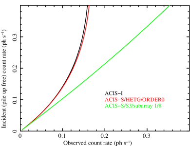
Figure 1: Relation between the incident $2-8$ keV count rate (as observed in absence of pile-up) and the actual observed $2-8$ keV count rate for three different observing modes often used during the Chandra observations. These relations are derived from the same pile-up models employed in the Chandra webpimms tool. For the computation we assumed the ”absorbed power-law” spectral model (Nowak et al. 2012) and 5 active chips (for the ACIS-I and ACIS-S 0^th-order observations). Because of the pile-up effect, with either ACIS-I or ACIS-S with no subarray, the observed count rate can not effectively be higher than $0.18$ ph s^-1, even for incident count rates $>0.2$ ph s^-1.

During the brightest flares the Chandra light curves are significantly affected by pile-up, if no subarray is used. Figure 1 shows the relations between the incident count rate, as observed if no pile-up effect is present, and the observed (piled-up) count rate. This conversion is accurate for the absorbed power-law model. We note that the pile-up effect becomes important ($\sim 5$ %) for count rates higher than 0.04 ph s^-1, well above the quiescent level. Therefore, pile-up does not affect the detection of flares or the determination of the flaring rate. It does, however, significantly affect the observed peak count rates and, therefore, the observed fluences of moderate, bright and especially very bright flares. Indeed, during either ACIS-I or ACIS-S 0^th-order observations it is very hard to characterise exceptionally bright flares with Chandra if no subarray or gratings is employed. For example, flares with incident peak count rates between $0.25$–$1.0$ ph s^-1 would produce an observed (piled-up) count rate between $\sim 0.14$–$0.17$ ph s^-1, never higher than $0.18$ ph s^-1, if no subarray (or grating) is used (see black and red lines in Fig. 1). In particular, we note that the two exceptionally bright flares detected in fall 2013 and fall 2014, with peak count rates of $\sim 0.5$–$1$ ph s^-1, respectively, would be heavily piled-up if no subarray were used, giving an observed (piled-up) count rate of $\sim 0.16$–$0.18$  ph s^-1. Some of the bright flares detected by Chandra, in observations with no subarray, could therefore actually be associated with very bright flares. The relation shown in Fig. 1 is based on the same pile-up model also employed in the webpimms tool. We correct the light curves, the Bayesian block results (see § 4) and the flare fluences for the pile-up effect by converting the observed count rates to the intrinsic count rates, using the curves shown in Fig. 1 (see also Tab. 1). As it can be seen in Fig. 1, as long as the observed count rates are lower than $\sim 0.12$ ph s^-1 the correction for pile-up is accurate, in fact the relations between incident and observed count rates are well behaved. For higher count rates in observations with no subarray, the relation becomes very steep, therefore it becomes increasingly difficult to determine the true incident count rate from the observed one. We a posteriori observe that a block count rate higher than 0.12 ph s^-1 is observed only during the very bright flare observed during obsID 1561 (Baganoff et al. 2001).

In grating observations, the comparison between the un-piled first-order photons, with the 0^th-order photons provides a recipe to correct count rates and fluences for the effect of pile-up, also for the luminous events (see Nielsen et al. 2013). We observe a posteriori that our method provide similar results to the one employed by Nielsen et al. (2013).

2.3 Comparison of count rates and fluences between different instruments

To enable the comparison between the light curves or fluences of flares observed by different instruments, we convert the observed corrected count rates and fluences from photon numbers into photon energies (in ergs). We assume, as established by previous analyses, that all flares have the same absorbed power-law shape with spectral index $\Gamma=2$ and are absorbed by a column density $N_{H}=1.5\times 10^{23}$ cm^-2 of neutral material (Porquet et al. 2008; Nowak et al. 2012). Using this model, we convert for each count rate and flaring block (see § 4) the ”corrected” count rate and block count rate into a flux (using webpimms⁵) and then use these to compute the fluences in ergs and plot the combined light curves (see Fig. 3 and 4). All count rates, fluxes and fluences correspond to the absorbed values. The value displayed in the last column of Tab. 1 shows the conversion factor.

Pile-up correction and conversion factors
Data Mode	p1	p2	p3	p4	CF
ACIS-I	1.563	1.099	1185	4.866	$4.2\times 10^{-11}$
ACIS-S HETG 0th	802.0	4.743	1.599	1.110	$1.0\times 10^{-10}$
ACIS-S HETG 0+1st					$5.83\times 10^{-11}$†
ACIS-S 1/8 subarray	0.2366	6.936	1.393	1.179	$4.09\times 10^{-11}$
EPIC-pn	1	1	0	0	$1.3\times 10^{-11}$

Table 1: Best fit conversion factors, for each instrument and observing mode, between observed count rates (affected by the pile-up effect) into unpiled-up count rates. The factors are derived using the webpimms estimates and are in the form: $cr_{int}(t)=p1\times cr_{o}(t)^{p2}+p3\times cr_{o}(t)^{p4}$, where $cr_{o}(t)$ is the observed count rate and $cr_{int}(t)$ is the intrinsic count rate, once corrected for the pile up effect. The last column shows the conversion factor (CF) used to transform the corrected count rate into a 2–10 keV flux (from ph s^-1 into erg cm^-2 s^-1). The conversion factor applied to the Chandra data is appropriate for unpiled up light curves in the 2–8 keV band. †See Nowak et al. (2012) and Neilsen et al. (2013).

2.4 Classification of flares

Definition flares types
Flare type	Fluence
	($10^{-9}$ erg cm-2)
Very bright	$F>20$
Bright	$5<F\leq 20$
Moderate	$1.5<F\leq 5$
Weak	$F\leq 1.5$

Table 2: Classification of different flares of Sgr A^⋆, according to the total observed (absorbed) flare fluence in the 2-10 keV energy band. We detect 20, 36, 16 and 8 weak, moderate, bright and very bright flares, respectively (the number of weak and moderate flares is incomplete).

This work aims at studying the long term trend in Sgr A^⋆’s flaring rate. To this end, we consider data from both the XMM-Newton and Chandra monitoring campaigns, regardless of the instrument mode used. This has the advantage of increasing the total exposure, therefore to provide a larger number of flares. However it has the disadvantage of producing an inhomogeneous sample. In fact, due to the different background levels of the various cameras and observation configurations employed, as well as the diverse point spread functions of the different satellites, the detection threshold to weak flares varies between observations and, in particular, between different satellites. Therefore, we divide the observed flares into four categories (ranked according to increasing fluence), weak, moderate, bright and very bright flares. The thresholds between the various categories are chosen primarily to select homogeneous samples of flares (e.g. observable by all satellites, by all instrumental mode of one satellite, etc.), but also to sample the fluence distribution with similar portions. Bright and very bright flares shall be the flares with fluence in excess of $5\times 10^{-9}$ and $20\times 10^{-9}$ erg cm^-2, respectively. These flares are detectable by both XMM-Newton and Chandra, in any observation mode employed, given the observed distribution of flare duration (Neilsen et al. 2013). Moderate flares are defined as those with fluences between $1.5\times 10^{-9}$ and $5\times 10^{-9}$ erg cm^-2. These are easily detectable with Chandra in any instrument set-up, while the high contribution from diffuse emission hampers the detection of a significant fraction of moderate flares by XMM-Newton. Therefore, we will only use Chandra for their study. We consider a weak flare as any significant variation, compared to quiescence, with a total fluence lower than $1.5\times 10^{-9}$ erg cm^-2. We note that the various Chandra instrumental set ups also have different thresholds for the detection of weak flares, with different levels of completeness.

In summary, observations performed both by XMM-Newton and/or Chandra give us a complete census of bright and very bright flares. On the other hand, to have a complete census of moderate flares, we restrict ourselves to Chandra observations only.

3 The 2013-2014 XMM-Newton monitoring of SGR A^⋆

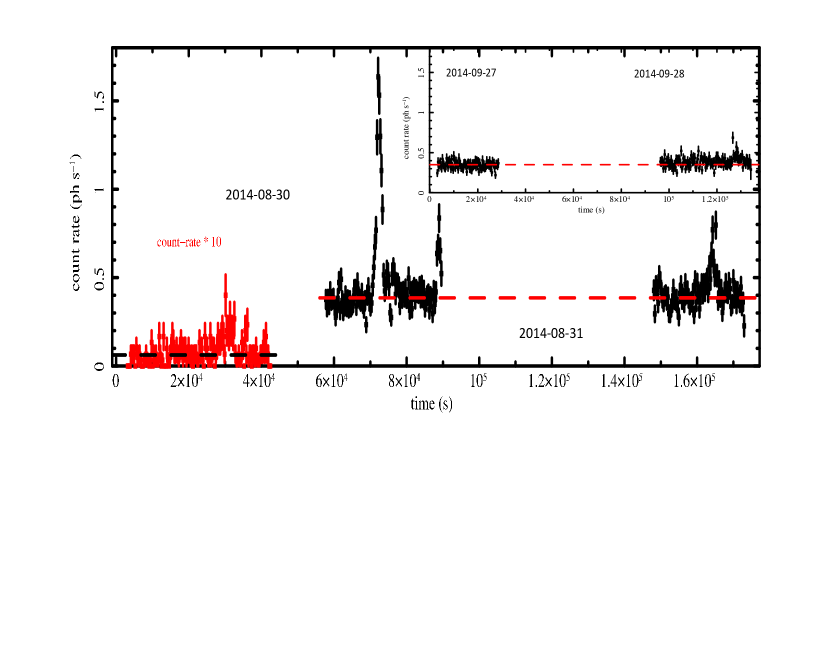
Figure 2: XMM-Newton and Chandra observations accumulated in fall 2014 are shown in black and red, respectively. For display purposes the Chandra count rate has been multiplied by 10. Four bright or very bright flares are clearly detected within the 4 XMM-Newton observations. An additional, but weaker, flare is observed during the earlier Chandra observation. The dashed line shows the best fit of a constant to the light curves after excluding the detected flares. The constant level observed by XMM-Newton follows the decay of the emission from SGR J1745-2900.

We start the investigation from the presentation of the new XMM-Newton data of the intensified monitoring campaign of Sgr A^⋆, obtained for the peri-center passage of G2. Three XMM-Newton observations were accumulated in fall 2013, in particular, on August 30, and September 10 and 22. Each light curve can be fitted with a constant flux of 0.924, 0.824 and 0.815 ph s^-1, respectively. We observe no obvious flare activity in any of the three light curves. However, our ability to detect moderate or bright flares is hampered by the increased flux induced by the outburst of the magnetar SGR J1745-2900, lying within the extraction region of the source light-curve (see § 2.1). The flux evolution between the different observations follows the typical exponential decrease observed in magnetars’ outbursts (Rea & Esposito 2011; Coti Zelati et al. 2015). Because the dominant contribution from this source prevents us from detecting even bright flares from Sgr A^⋆, we decided to discard these observations.

The light curves of the four XMM-Newton observations obtained on August 30, 31, September 27 and 28, 2014 (black data-points in Fig. 2) instead show four bright flares (with fluence of 289.4, 62.5, 102.2 and $58.8\times 10^{-10}$ erg cm^-2) above the constant level of emission characterising Sgr A^⋆’s quiescent level. Fitting the light curves with a constant, after excluding the flaring periods, returns count rates of 0.411, 0.400, 0.339, and 0.378 ph s^-1, respectively, for the four different XMM-Newton observations. The extrapolation of the long-term flux evolution of the magnetar, as measured by Chandra, as well as the comparison of the new XMM-Newton data with archival observations, suggests that the magnetar contributes at the level of $\sim 50$% to the observed quiescent flux (the observed count rate before the magnetar’s outburst was 0.196 ph s^-1).

3.0.1 Can the magnetar be responsible for the flares observed with XMM-Newton?

On top of their bright persistent X-ray emission, magnetars show very peculiar flares on short timescales (from fraction to hundreds of seconds) emitting a large amount of energy ($10^{37}-10^{46}$ erg s^-1). They are probably caused by large scale rearrangements of the surface/magnetospheric field, either accompanied or triggered by fracturing of the neutron-star crust, as a sort of stellar quakes. Furthermore, magnetars also show large outbursts where their steady emission can be enhanced up to $\sim$1000 times its quiescent level (see Mereghetti 2008; Rea & Esposito 2010 for recent reviews). From the phenomenological point of view, the bursting/flaring events can be roughly divided in three types: i) short X-ray bursts, these are the most common and less energetic magnetar flares. They have short duration ($\sim 0.1-0.2$ s), and peak luminosity of $\sim 10^{37}-10^{41}$ erg s^-1. They can be observed in a bunch as a flaring forest, or singularly; ii) Intermediate flares (in energy and duration with the flare classes) have typical durations from a few to hundreds of seconds, and luminosities $\sim 10^{39}-10^{43}$ erg s^-1; iii) Giant flares are by far the most energetic Galactic flare ever observed, second only to a possible Supernovae explosion. The three giant flares detected thus far were characterised by a very luminous hard peak lasting a bit less than a second, which decays rapidly into a hundreds of seconds tail modulated by the magnetar spin period.

Given the vicinity between SGR J1745–2900 and Sgr A^∗ ($\sim 2.4$”; Rea et al. 2013), they both lay within the XMM-Newton point spread function. Being both flaring sources, we try to use physical and observational constraints to exclude that the apparent excess in the flaring activity observed by XMM-Newton from the direction of Sgr A^∗ might be due instead to magnetar flares.

Given the duration and luminosities of the X-ray flares detected by XMM-Newton (see Neilsen et al. 2013), the most similar magnetar flare that we need to exclude is of the class of intermediate flare. Magnetars’ intermediate flares are usually observed from young and highly magnetised members of the class (as it is the case of SGR J1745–2900), either as several consecutive events or singularly (Israel et al. 2008; Woods et al. 2004). Their spectra are best fit with a two blackbody model, with temperatures of $kT_{1}\sim 0.5-5$ keV and $kT_{2}\sim 6-20$ keV, from emitting regions of $R_{1}\sim 10-30$ km and $R_{2}\sim 0.1-10$ km, and luminosities of the order of $10^{38}-10^{42}$ erg s^-1. We then studied in detail the light-curves and the spectra of our flares. The spectra of all flares were fitted with a two blackbody model finding a good fit with temperatures of the order of $kT_{1}\sim 0.7$ keV and $kT_{2}\sim 6.5$ keV. Although the spectral decomposition might resemble that of a typical magnetar intermediate flare, the derived luminosities of $\sim 10^{35}-10^{36}$ erg s^-1 are low for a magnetar flare. Furthermore, we find durations around thousands of seconds, which are also rather long for a magnetar flare.

Even though we cannot distinguish spatially in our data the magnetar from Sgr A^⋆, we are confident that the flaring activity we observe in our XMM-Newton observations are not generally consistent with being due to SGR J1745–2900 and they are produced by Sgr A^⋆.

3.0.2 A-posteriori probability of observing the detected flares

The observation of four bright or very bright flares in such a short exposure ($\sim 130$ ks) is unprecedented. Following a $\sim 3$ Ms Chandra monitoring campaign, Neilsen et al. (2013) estimated Sgr A^⋆’s flaring rate and the fluence distribution of the flares. With a total of 39 observed flares, they infer a mean flaring rate of $\sim 1.2$ flares per 100 ks.

In particular, we note that only nine bright or very bright flares (according to the flare definition in Tab. 2) were detected during the 3 Ms Chandra monitoring campaign. Assuming a constant flaring rate, 0.4 such flares were expected during the 133 ks XMM-Newton observation, as compared to the four that we observed.

We note that Chandra was observing Sgr A^⋆ less than 4 hours before the start of the XMM-Newton observation on August 30, 2014. The red points in Fig. 2 show the Chandra light curve, rescaled by a factor 10 for display purposes. A weak flare is clearly observed during the $\sim 35$ ks exposure. An additional $\sim 35$ ks Chandra observation was performed on October 20, 2014, about one month after the last XMM-Newton pointing. A very bright, as well as a weak flare were detected during this observation (see Figs. 3 and 4, Tab. 5 and Haggard et al. 2015). Therefore a total of five bright or very bright flares have been observed within the 200 ks XMM-Newton and Chandra monitoring campaign performed at the end of 2014, while an average of only 0.6 bright flares would have been expected, based on the bright flaring rates previously established (Neilsen et al. 2013; 2015; Degenaar et al. 2013).

Assuming that the flaring events are Poisson distributed and that the flaring rate is stationary, we find an a posteriori probability $P=Poiss_{0-3}\left({\lambda}\right)=0.07$ % of observing four or more bright flares during the XMM-Newton observations, and a probability of $0.04$ % of observing five or more bright flares in 200 ks. These estimates suggest (at just above $3\sigma$ significance) that the observed increase of flaring rate is not the result of stochastic fluctuations. Thus, either bright flares tend to cluster, or the flaring activity of Sgr A^⋆ has indeed increased in late 2014.

This suggestive change in flaring rate is strengthened by considering also Swift observations. Between 2014 August 30 and the end of the Swift visibility window (on November 2^nd), Swift observed Sgr A^⋆ 70 times for a total of 72 ks. On September 10, Swift detected a bright flare, strengthening the indication of clustering and/or increased flare activity during this period (Reynolds et al. 2014; Degenaar et al. 2015).

Considering all observations of XMM-Newton, Chandra and Swift carried out between mid August and the end of the 2014 Sgr A^⋆’s observability window, a total of six bright flares were detected within 272 ks of observations, with associated Poissonian probability of $2\times 10^{-4}$ (about $3.8\sigma$ significance). However, before jumping to any conclusion, we note that the estimated probability critically depends on the a-posteriori choice of the ”start” and duration of the monitoring interval considered. To have a more robust estimate of this probability we need to employ a well-defined statistic to rigorously identify flares, and then to apply a method capable of measuring variations in the flaring rate, without making an a-posteriori choice of the interval under investigation. To do so, we perform a Bayesian block analysis.

4 Bayesian Block analysis

To have a robust characterisation of Sgr A^⋆’s emission we divide all the observed light curves into a series of Bayesian blocks (Scargle et al. 2013; see also Nowak et al. 2012). The algorithm assumes that the light curve can be modeled by a sequence of constant rate blocks. A single block characterises light curves in which no significant variability is detected. Significant variations will produce blocks with significantly different count rates and separated by change points. The over-fitting of the light curve is controlled by the use of a downward-sloping prior on the number of blocks.

4.1 Bayesian block algorithm

We use the implementation of the ”time tagged” Bayesian block case described by Scargle et al. (2013) and provided by Peter K.G. William. The code employs a Monte Carlo derived parameterisation of the prior on the number of blocks, which is computed from the probability $p0$, given as an estimation of false detection of an extraneous block (typically set at 5 % Williams et al. 2014; Scargle et al. 2013). The algorithm implements an iterative determination of the best number of blocks (using an ad hoc routine described in Scargle et al. 2013) and bootstrap-based determination of uncertainties on the block count rate. This implementation starts from the un-binned, filtered Chandra event file in FITS format. We modified the algorithm to read XMM-Newton event files as well. The errors and probabilities of false detection presented in this paper are derived from independent procedures described in § 5.1 and 5.5.

4.2 Definition of flare, time of the flare, start and stop time, duration and fluence

We define flares as any Bayesian block with count rate significantly different from the one(s) describing the quiescent level (we assume that the quiescent emission is constant within each observation). The low flaring rate typical of Sgr A^⋆ allows a good characterisation of the quiescent level in all the light curves analysed. Most of the flares are characterised by only one flaring block (i.e., a simple rise to a peak value and then a fall back to the quiescent level). However, bright or very bright flares can present significant substructures generating more than one flaring block for each flare. Long bright flares can easily be disentangled from a series of several distinct flares, because the latter have a non-flaring block separating the flares. For each flare, we define as the flare start and stop time the first and the last of the change points characterising the flaring blocks. The flare duration shall be the sum of the durations of the flaring blocks. The flare time shall be the mid point of the flaring block with the highest count rate. This definition is also applied if a flare is in progress either at the start or at the end of the observation. We compute the fluence in each flaring block starting from the flare count rate during the flaring block, once corrected for pile-up and converted to a flux. To remove the contribution from background emission, contaminating point sources (e.g. SGR J1745-2900, CXO-GC J174540.0-290031) and different levels of diffuse emission (induced by the different PSF), we subtract the quiescent blocks count rate (averaged over all the quiescent blocks of the observation under investigation) from the count rate of the flaring block. We then obtain the fluence of each flaring block by multiplying the ”corrected flare” block count rate by the block duration. The total flare fluence shall be the sum of the fluences of all the flaring blocks composing the flare (see last column of Tab. 4, 5, 6 and 7).

4.3 Results

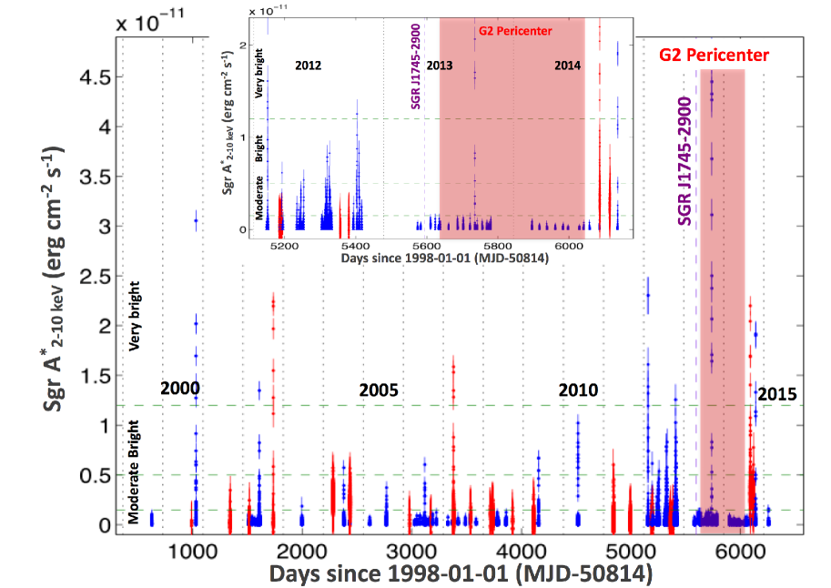
Figure 3: (Main figure) XMM-Newton (red) and Chandra (blue) coverage of X-ray emission from Sgr A^⋆. Each blue or red point corresponds to a bin of 300 s and shows the flux (with the conversion factors shown in Tab. 1) measured by either Chandra or XMM-Newton, once corrected for the pile-up effect (see § 2.2.1 and Tab. 1). Flares are manifested as rapid and significant deviations from the quiescent level. The quiescent level of emission observed by XMM-Newton fluctuates (see red data points) because of the contribution from point sources within the extraction region chosen for this instrument (see § 2). The dotted lines correspond to the yearly separation. From 2001 to 2005 only sporadic observations were performed. In 2006-2008 several observations were performed. The long 2012 XVP as well as the 2013-2014 monitoring are now allowing good characterisation of the evolution (if any) of the X-ray properties over time-scales of a year. The start of the outburst of SGR J1745-2900 is marked with a violet dashed line. The pink box indicates the approximate time of the passage of G2 at peri-center. (Upper panel) Zoom of the last three years of monitoring. Several bright-or-very bright flares are observed at the end of 2014, with a higher frequency compared to previous observations. No moderate or bright flare is observed between the beginning of 2013 and mid 2014, in contrast to the frequent occurrence of moderate flares observed in 2012.

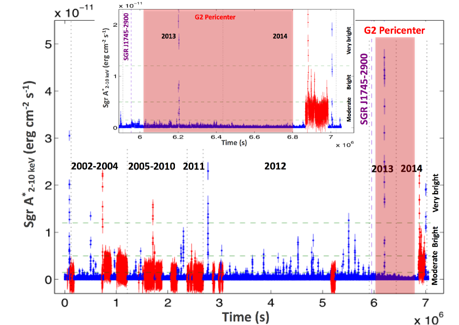
Figure 4: (Main figure) XMM-Newton (red) and Chandra (blue) light curves of the 2–10 keV flux emitted by Sgr A^⋆. Gaps between observations are removed. Dotted black vertical lines separate the different years or periods. The longest total exposure was obtained in 2012. The dashed violet vertical line indicates the start of the outburst of the magnetar SGR J1745-2900 on 2013 April 25 (§ 2.1). The pink box indicates the approximate time of the peri-center passage of G2 (Gillessen et al. 2013; Witzel et al. 2014). The dashed green horizontal lines roughly indicate the demarcation between weak, moderate, bright and very bright flares. The different flare types are defined here on the basis of their fluence and not by their peak count rates. The thresholds between weak and moderate and between moderate and bright flares indicate the average count rate for flare lengths of 1 ks. Longer flares lasting 1.7 ks are considered for displaying the threshold between the bright and very bright flares. The brightest flare has been detected on 2013 September 14 (Haggard et al. 2015). We note that, before 2013, weak, moderate and bright flares are randomly distributed within the 15 years of observations. This Sgr A^⋆ light curve suggests a lack of moderate flares during 2013 and 2014, while we observe a series of 5 bright flares clustering at the end of 2014, several months after the peri-center passage of the bulk of G2’s material. (Upper panel) Zoom on the 2013-2014 period that shows that no moderate flare was observed, while 5 bright flares were observed right at the end of the XMM-Newton and Chandra monitoring campaigns. An additional bright flare (not shown here) was detected by Swift on October 10, 2014, right in the middle of the XMM-Newton monitoring campaign. These observations suggest an increased flaring rate of Sgr A^⋆ during fall 2014.

Figures 3 and 4 show the Chandra and XMM-Newton light curves of Sgr A^⋆ in blue and red, respectively. We present here, for the first time, the light curves accumulated since 2013. These have been obtained in the course of large Chandra and XMM-Newton monitoring campaigns aimed at studying any variation in the emission properties of Sgr A^⋆ induced by the close passage of the G2 object (PIs: Haggard; Baganoff; Ponti). A detailed study of the possible modulation of the quiescent emission, induced by the passage of the cloud, is beyond the scope of this paper and will be detailed in another publication. Here we focus our attention on the flaring properties only. A total of 80 flares have been detected in the period between 1999 and 2014 (11 by XMM-Newton in 1.5 Ms; 20 by Chandra between 1999 and 2011, in 1.5 Ms; 37 by Chandra in 2012, 2.9 Ms; 12 by Chandra between 2013 and 2014, in 0.9 Ms). The details of all observations, of all flaring blocks and all flares are reported in Tables 4, 5, 6 and 7.

The first systematic study of the statistical properties of a large sample of Sgr A^⋆’s flares was published by Nielsen et al. (2013). The authors analysed the 38 Chandra HETG observations accumulated in 2012 with a total exposure of $\sim 3$ Ms and employed two methods to detect flares. Through an automatic Gaussian fitting technique, the authors detected 39 flares and provided full details for each flare (see Tab. 1 of Neilsen et al. 2013). Thirty-three flares are in common. We detect five flares, missed by the Gaussian fitting method employed by Nielsen et al. (2013). These flares are characterised by low rates (in the range $0.01-0.005$ ph s^-1) and long durations (lasting typically $3-13$ ks), therefore are easily missed by the Gaussian method more efficient in detecting narrow-peaked flares. On the other hand, our method misses seven flares detected instead by Neilsen et al. (2013). Our smaller number of detected flares is a consequence of limiting our study to the zeroeth order (ACIS-S), therefore to smaller statistics (indeed the 7 flares missed, are within the weakest ones detected by Neilsen et al. (2013), in particular all those having fluences lower than 23 photons). Neilsen et al. (2013) also employ a different technique to detect flares based on a Bayesian block algorithm resulting in the detection of 45 flares. The various methods provide consistent results for moderate, bright and very bright flares and only differ in the detection of weak flares.

At first glance, no variation on the flaring rate appears evident before and during the peri-center passage of G2. On the other hand, three flares, including a very bright one, were detected about 6 months after peri-center passage (see Tab. 6).

4.4 Distribution of flare fluences

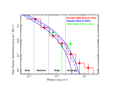
Figure 5: Distribution of flare rate as a function of fluence (in erg cm^-2 Ms^-1), as observed during 15 years of Chandra (red) and XMM-Newton (green) monitoring. The blue dashed and solid curves indicate the best-fit and 1-$\sigma$ uncertainties on the fluence distribution observed during the Chandra XVP campaign in 2012 (Neilsen et al. 2013). The vertical dotted lines indicate the fluence intervals characterising the various types of flares (see Tab. 2).

The red points in Fig. 5 show the distribution of flare fluences (normalised to 1 Ms) observed by Chandra over the past 15 years, while the blue dashed and solid lines show the best fit and 1-$\sigma$ uncertainties on the fluence distribution estimated from the Chandra XVP campaign in 2012 (Neilsen et al. 2013). We observe remarkably good agreement between the two. In particular, even if we did not correct the flaring rate for completeness (particularly important for weak flares), the agreement at low fluences indicates that Chandra (ACIS-I and ACIS-S with no gratings) and XMM-Newton are complete in detecting moderate-or-bright and bright-or-very bright flares, respectively. In addition, we note that both XMM-Newton and Chandra show a subtle deviation, suggesting a higher number of very bright flares is observed during the entire dataset analysed, as compared to the 2012 Chandra campaign only. This excess might be a result of the inclusion of the latest 2013-2014 campaign.

5 Variation of the flaring rate?

The Bayesian block analysis of the XMM-Newton and Chandra light curves confirms the presence of several bright-or-very bright flares occurring at the end of 2014 and allows us to measure the basic flare characteristics. To check for any variation of the flaring rate, in an independent way from the a posteriori choice of the start of the interval under investigation (see discussion in Section 3), we consider each flare as an event and then we apply the Bayesian block method to measure any variations of the event rate.

5.1 MonteCarlo simulations to estimate the uncertainties on flaring rates in a given time bin

We estimate the uncertainty on the number of flares that we expect over a given observing time interval, and therefore on the flaring rate, based on Monte Carlo simulations. The simulations are performed assuming that the flares follow the fluence distribution as observed during the Chandra XVP campaign and reported in Fig. 5 (blue dashed line, see also Neilsen et al. 2013). We first compute the integral of the flare fluence distribution to estimate the total number, N_tot, of flares expected for the entire duration of the monitoring (XMM-Newton, Chandra and Swift 2014). Assuming that the flares are randomly and uniformly distributed in time we simulated N_tot flare occurrence times. Then, for each time interval under consideration (i.e. covering the duration of the monitoring from a single, or a combination of more observatories), we count the number of simulated random occurrences, $N_{sim}$, within that interval. We randomize the fluences of the $N_{sim}$ flares within each interval, by drawing $N_{sim}$ random numbers from the ChandraXVP fluence distribution. Of these we consider only a given class of flares (e.g. bright and very bright) and derive a simulated flare rate associated with this class. We repeat this procedure $10^{3}$ times, and estimate the corresponding standard deviation of flare rate. Finally, we use this value as the uncertainty associated with the observed rate of the given class of flares and within each time interval of interest.

5.2 Chandra observed flaring rate

	Chandra 2012	Chandra 1999-2014	XMM-Newton 2000-2014	XMM-Newton +
			[2000-2012] [Aug-Sep 2014]	Chandra (1999-2014) + Swift (2014)
All flares	$1.08\pm 0.10$
Bright-Very Bright	$0.26\pm 0.05$	$0.26\pm 0.02$	$0.45\pm 0.16[0.25\pm 0.10][2.6\pm 1.3]$	$0.27\pm 0.01/2.52\pm 0.98$‡
Moderate-Very Bright	$0.97\pm 0.12$	$0.82\pm 0.05$
Moderate-Bright	$0.76\pm 0.12$	$0.69\pm 0.07/0.11\pm 0.05$†
Moderate	$0.70\pm 0.11$	$0.67\pm 0.07/0.11\pm 0.05$†

Table 3: Flaring rates (day^-1) for different types of flares as observed by Chandra and XMM-Newton during different observing intervals. When a variation of the flaring rate is observed, the flaring rate of the two blocks are reported. For XMM-Newton we report also (in parentheses) the flaring rate observed before the end of 2012. †The change point (variation in the flaring rate) is observed on June 5, 2013. ‡The change point is observed on August 31, 2014.

We first compute the flaring rate during the 2012 Chandra observations only ($2.9$ Ms exposure). We observe a rate of all flares (from weak to very bright) of $1.08\pm 0.10$ per day, and $0.26\pm 0.05$ bright or very bright flares per day (see Tab. 3). These values are consistent with the numbers reported by Neilsen et al. (2013; 2015).

To expand the investigation to Chandra observations performed with a different observing mode, we henceforth discard the weak flares. Taking all new and archival Chandra observations from 1999 until the end of 2014 ($\sim 5.3$ Ms exposure), we observe that the rate of moderate-to-very-bright flares has a mean value of $0.82\pm 0.05$ flares per day (a rate of $0.97\pm 0.12$ was observed during 2012), while the rate of bright-or-very bright flares is $0.26\pm 0.02$ per day. Restricting this investigation to the Chandra data only (with $p0<0.05$), no significant difference in the rate of total flares is observed.

Despite the invariance of the total flare rate over the 15 years of Chandra observations, we note a paucity of moderate flares over the 2013-2014 period, compared to previous observations (see Fig. 4). Indeed, the rate of moderate flares was $0.67\pm 0.07$ per day, showing a tentative indication of a drop to $0.11\pm 0.05$ after June 5, 2013 (see Fig. 4; $p0=0.08$). Moderate flares, if present, would be detected even considering the additional contamination induced by SGR J1745-2900.

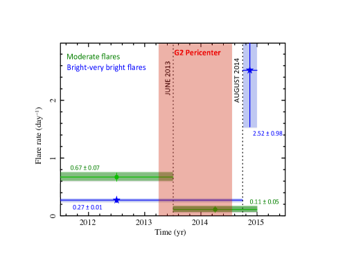
Figure 6: Zoom of the variation of the flaring rate of Sgr A^⋆ over the past 3.5 years. The green data points show the moderate-bright flaring rate (Chandra only), while the green regions indicate the modulation of the rate and its uncertainty ($1\sigma$) derived through Monte Carlo simulations (see §5.1). The moderate flaring rate is observed to be constant for more than a decade and to significantly (at the 96 % confidence level; see § 5.5) drop after 2013 June 5, several months before the peri-center passage of the bulk of G2’s material (see pink box). The blue data points show the bright and very bright flaring rate (Chandra and XMM-Newton) as derived from the combined Chandra, XMM-Newton and Swift observing campaigns over the past 15 years, while the shaded light blue regions show the uncertainties (see § 5.1). After being constant for more than 14 years, the bright-or-very bright flaring rate significantly ($\sim 99.9$ % confidence level) increased after 2014 August 31, several months after the peri-center passage of G2.

5.3 Flaring rate observed with XMM-Newton

The total cleaned exposure of the entire XMM-Newton monitoring of Sgr A^⋆ (from 2000 until the end of 2014) is composed of about $1.6$ Ms of observations. We detected eleven flares. This lower number compared to Chandra can be attributed to the inability of XMM-Newton to detect weak and moderate flares. Eight either bright or very bright flares are detected by XMM-Newton, resulting in a mean rate of $0.45\pm 0.16$ bright flares per day (see Tab. 3). This rate is higher than the one measured by Chandra. This is due to the 4 bright or very bright flares detected during the observations accumulated in fall 2014. In fact, if only the observations carried out before the end of 2012 are considered, the rate of bright or very bright flares drops to $0.25\pm 0.10$ per day, consistent with the rate derived with Chandra and seen with Swift in 2006-2011 (Degenaar et al. 2013). On the other hand, if we consider only the XMM-Newton observations carried out in August and September 2014, the observed rate is $2.6\pm 1.3$ per day.

5.4 XMM-Newton, Chandra and Swift light curves to constrain the change of the rate of bright flares

Combining the light curves of XMM-Newton, Chandra and Swift (2014) we obtain a total cleaned exposure time of $\sim 6.9$ Ms. During this time, 30 bright-or-very bright flares were detected.

The Bayesian block analysis now significantly detects a variation in the rate of bright or very bright flares in late 2014. In particular, a constant flaring rate, from 1999 until summer 2014, of $0.27\pm 0.01$ bright flares per day, is found. On August 31, 2014 we find a change point in the flaring rate such that the rate significantly increased to $2.52\pm 0.98$ per day (see Tab. 3), a factor $\sim 10$ higher than the prior value (see Fig. 6). This variation of the flaring rate is not detected by the Bayesian block routine if we require a value of $p0$ smaller than 0.003.

The point in time when the variation of the flaring rate occurred (change point) is quite precise (the typical spacing between the 2014 XMM-Newton and Chandra observations is of the order of $1$ month) and took place several months after the bulk of the material of G2 passed peri-center. In particular no increase in the flaring rate is observed 6 months before (e.g. in 2013) and/or during the peri-center passage (Gillessen et al 2013; Witzel et al. 2014).

5.5 Significance of the flaring rate change

To give a rigorous estimate of the probability of detecting a variation in the bright and very bright flaring rate of Sgr A^⋆, we performed MonteCarlo simulations. In the simulations we assumed a constant flaring rate, and the fluence distribution observed by Chandra in 2012 (see Fig. 5 and Neilsen et al. 2013). The latter was used to derive the expected total number, N, of bright and very bright flares in the hypothesis that the flaring rate did not change since 2012. Assuming that the flares are randomly and uniformly distributed (such that any clustering which would produce an increase of flaring rate occurs by chance), we simulated N occurrence times for the bright and very bright flares over a total exposure which corresponds to the duration of the combined Chandra, XMM-Newton and Swift (2014) campaigns. We repeated this procedure $10^{4}$ times, each time applying the Bayesian block algorithm (with p0=0.003) to measure how often the Bayesian method detects a spurious increase of the flaring rate. This happened 10 times out of $10^{4}$ simulations. Therefore the significance of the detected variation in Sgr A^⋆’s bright and very bright flaring rate is $\sim 99.9$ % ($\sim 3.3\sigma$). The presence of observing gaps does not affect the estimated probability (if the flaring rate is constant, e.g., if the flare occurrence times are uniformly distributed).

In the same way, to estimate the significance of the variation of the moderate-or-bright flares, we simulated $10^{4}$ light curves with an exposure as observed within the Chandra campaign. From these we selected the moderate-or-bright flares only, then we applied the Bayesian block algorithm with $p0=0.08$, such as observed in § 5.2. We observe that spurious variations happened 394 times, suggesting a significance of the variation of the moderate flares at the $96$ % confidence level.

6 Variation of the total luminosity emitted as bright-or-very bright flares

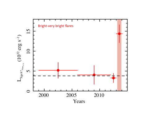
Figure 7: Light curve, over the 15 years of XMM-Newton and Chandra monitoring, of the total luminosity emitted by Sgr A^⋆ as bright or very bright flares. A constant luminosity is observed up to the end of 2012 (see dashed line). A significant ($\sim 3.5$–$\sigma$ confidence) increase, by a factor $\sim 3.7$, is observed during the years 2013-2014. Error bars indicate the 1-$\sigma$ uncertainty as derived in § 6. The pink region indicates the period of peri-center passage of G2.

Figure 7 shows the light curve, over the past 15 years of XMM-Newton and Chandra monitoring, of the average luminosity emitted by Sgr A^⋆ in the form of bright-or-very bright flares. We choose a single time bin for the long XMM-Newton and Chandra exposure in 2012 and one for the 2013-2014 campaign, while we divide the historical monitoring from 1999 to 2011 in two time bins, having roughly similar exposures. The amplitude of the uncertainty on the measurement of the energy released by Sgr A^⋆, in the form of flares, depends both on the uncertainty on the measurement of the energetics associated with each single flare and on the uncertainty on the number of flares that we expect in the given interval. The first one can be estimated through error propagation and it is typically negligible compared to the second, given the flare distribution and the intervals considered here. We estimate the uncertainty on the total luminosity in flares over a given interval through the same procedure as described in section 5.1.

Sgr A^⋆ shows an average luminosity in bright-or-very bright flares of $L_{\rm Fx_{BVB}}\sim 3.8\times 10^{32}$ erg s^-1 (assuming a 8 kpc distance) over the 1999-2012 period (see Fig. 7). No significant variation is observed. On the other hand, a significant increase, compared to a constant ($\sim 3.5\sigma$ confidence; $\Delta\chi^{2}=19.6$ for 3 dof), of a factor of 2-3, in Sgr A^⋆’s luminosity is observed over the 2013-2014 period (see Fig. 7). This result, such as the variation of the flaring rate, suggest a change in Sgr A^⋆’s flaring properties.

6.1 Historical and new fluence distribution

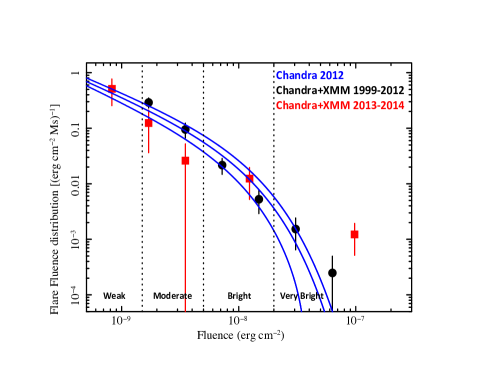
Figure 8: Change of the distribution of the flare rate as a function of fluence (in erg cm^-2 Ms^-1), as observed during 15 years of Chandra and XMM-Newton monitoring. The flare fluence distribution observed during the 1999-2012 period (black circles) is consistent with that observed during the XVP campaign (blue lines). A variation of the flare fluence distribution has been observed during the past two years (red squares). In particular, both a larger number of very bright flares (and possibly fewer moderate flares) have been observed. The dotted vertical lines indicate the different types of flares. 1–$\sigma$ uncertainties are displayed.

The black circles in Fig. 8 show the flare fluence distribution as observed during the 1999-2012 period. The XMM-Newton and Chandra monitoring campaigns, lasting for more than a decade show no significant variation of Sgr A^⋆’s flaring activity, compared to that observed in 2012 (Neilsen et al. 2013). On the other hand, during the past two years a significant change in the flare fluence distribution is observed. In fact, during the 2013-2014 period (see red squares in Fig. 8) the fluence distribution deviates from the one observed in 2012. In particular, we observe a clear increase in the number of very bright flares and the tentative detection of a decrease in the number of moderate flares, during the past two years. These results confirm the conclusions obtained through the study of the variation of the flaring rate and luminosity. Figure 8 shows that, despite the tentative detection of a decrease in the rate of moderate flares, the enhanced rate of very bright flares drives the observed increase of the total energy released by Sgr A^⋆.

7 Discussion

Through a Bayesian block analysis of Sgr A^⋆’s flaring rate light curve, we observe a $\sim 99.9$ % significance increase of the rate of bright or very bright flare production, from $0.27\pm 0.04$ to $2.5\pm 1.0$ day^-1, starting after summer 2014. We also observe a tentative detection ($\sim 96$ % significance) of a decrease in the rate of moderate-bright flares since mid 2013 (see Fig. 8 and 6). Despite the decrease in the rate of moderate flares, the total energy emitted by Sgr A^⋆, in the form of bright-or-very bright flares, increased (at $\sim 3.5\sigma$ confidence level) over the 2013 and 2014 period, compared to historical observations. The close time coincidence with the passage of G2 at peri-center is suggestive of a possible physical connection. Yet, since the power spectrum of the regular X-ray flaring activity is not well known and because of the frequent monitoring in this specific time period, one cannot exclude that the observed variation is a random event.

Is the observed flaring activity of Sgr A^⋆ an odd behaviour of a peculiar source? Has a similar change of the flaring rate ever been observed in other sources?

7.1 Comparison with quiescent stellar mass BH systems

Flaring activity is a common characteristic of the optical and infrared counterparts of compact binaries (see e.g. Bruch 1992), including quiescent stellar-mass BHs in X-ray binaries. In particular, Zurita, Casares & Shahbaz (2003) presented a detailed study of this topic, showing that intense flaring – amplitudes varing from 0.06 to 0.6 optical magnitudes – is systematically present in the light curves of four BH systems and one neutron star X-ray binary. These flares are bright enough to rule out a companion star origin, and therefore are believed to arise from the accretion flow. Flare durations range from a few hours down to the shortest sampling performed, typically of the order of minutes. The optical power density spectra show more power at low frequencies and can be modelled by a power-law with a spectral index of $\beta\sim$ –1 for three of the systems, and $\beta\sim$ –0.3 for the other, hence closer to white noise. High cadence observations of XTE J118+40; (Shahbaz et al. 2005) have shown that this power-law extends up to frequencies corresponding to time scales of at least a few seconds. The number of flares is witnessed to decrease with duration and long events tend to be brighter.

Interestingly, the long-term activity is known to vary in at least one of the BHs analysed (A0620–00), where active and passive quiescent states have been reported by Cantrell et al. (2008). The former are slightly brighter and bluer, whereas much weaker flaring activity is observed during the latter, when the light-curve is largely dominated by the modulation produced by the Roche-lobe shaped companion star. Typical time scales for these states go from a month to years, but transitions seem to occur in a few days.

Time resolved X-ray observations during quiescence have been also performed for the X-ray brightest of the above objects, V404 Cyg, which has a quiescent X-ray luminosity of $\sim 10^{34}$ erg s^-1 (see e.g. Hynes et al. 2004). We note that this is a factor $10^{2-4}$ brighter than typically observed for stellar-mass black holes in quiescence (see e.g. fig. 3 in Armas Padilla et al. 2014). Numerous X-ray flares with an amplitude of one order of magnitude in flux are observed, and they are correlated with optical events, with short-time time-lags that can be explained by X-ray (or Extreme Ultraviolet) reprocessing. X-ray flares have also been detected in some quiescent X-ray binaries with neutron stars accretors (e.g. Degenaar & Wijnands 2012).

This evidence is in line with the idea that flaring activity is not a peculiarity of Sgr A^⋆ (e.g. related to a process unique to supermassive BH environments), instead it appears to be a common property of quiescent BH (e.g. possibly related to the accretion flow). In particular, in V404 Cyg, the system with the brightest optical and X-ray quiescent level (therefore allowing the best multi-wavelength characterisation of the flaring activity) correlated optical and X-ray flares are observed (Hynes et al. 2004). In addition, no lag between the X-ray and optical variations are observed, implying that they are casually connected on short time-scales. This indicates that the optical and X-ray flaring activity are linked by a process generated in the inner accretion flow. Furthermore, the observed change in Sgr A^⋆’s flaring properties also appears compatible with the long term evolution of the flaring activity in binaries. However, we note that if flare durations linearly scale with BH mass, it is not possible to detail the flares of BH binaries on the same scaled times observed in Sgr A^⋆. Further analysis, which is beyond the scope of this work, is needed to actually probe that the same physical process is at work in both type of objects.

7.2 Clustering of bright flares: is it an intrinsic property of the underlying noise process?

The origin of Sgr A^⋆’s flaring activity is still not completely understood. The observation of bright flares is generally associated with the detection of few other weaker flaring events, suggesting that in general flares tend to happen in clusters (Porquet et al. 2008; Nowak et al. 2012). If so, the observed variation might be the manifestation of an underlying process that, although being stationary (showing the same average flaring properties on decades time-scales), produces flares not uniformly distributed in time.

Though uninterrupted XMM-Newton observations have already suggested a possible clustering of bright flares, only now we can significantly show that the distribution in time of bright flares is not uniform. Sgr A^⋆’s flaring activity, in the IR and sub-mm bands, is dominated by a red noise process at high frequencies, breaking at timescales longer than a fraction of a day (Do et al. 2009; Meyer et al. 2009; Dodds-Eden et al. 2011; Witzel et al. 2012; Dexter et al. 2014 Hora et al. 2014). Sgr A^⋆’s X-ray emission appears to be dominated by two different processes, one diffuse and constant, dominating during the quiescent periods, and one producing narrow, high-amplitude spikes, the so called flares. The power spectral shape of the latter is not clearly determined, however the X-ray light curves appear fairly different from the red-noise dominated light curves of AGN with comparable BH mass (Uttley et al. 2002; McHardy et al. 2006; Ponti et al. 2010; 2012).

A correlation is observed between the bright IR flux excursions and the X-ray flaring activity (although IR flares typically have longer durations), suggesting a deep link between the variability process in these two bands. X-ray flares might occur only during the brightest IR excursions, therefore happening more frequently when the mean IR flux results to be high because modulated by the intrinsic red-pink noise process in IR. If so, the observed variation in the X-ray flaring rate might suggest the presence of long term trends (on timescales longer than the typical X-ray observations) generally associated with red or pink (flicker) noise processes. In this case, the observed clustering would be an intrinsic property of the noise, and the variation would be detected significantly simply because of the increased frequency in monitoring of Sgr A^⋆, without a priori physical connection with the peri-center passage of G2. If this is indeed the case, we would expect that the next set of observations will show the same flaring rate as recorded in historical data, with another clustering event happening at some other random point in the future.

This is also in line with what is observed in other quiescent BH. Indeed, strong flaring activity has been observed in all quiescent stellar mass BH where this measurement was possible (Zurita et al. 2003). In particular, at least one object (the best monitored, A0620-00) showed a dramatic change in the flaring properties, with periods devoid of any observed flare followed by intense flaring episodes. Transitions between flaring and non-flaring periods occurred at irregular intervals of time-scales typically longer than a (few) day(s). Assuming that these time-scales vary linearly with the BH mass, we would expect to observe macroscopic changes in the flaring rate to occur on time-scales longer than many hundred years, or even longer period (and luminosity amplitudes smaller) than what is probed by GC molecular clouds (e.g. Sunyaev et al. 1993; Ponti et al. 2010; 2013; Zhang et al. 2015).

7.3 Enhanced flaring activity induced by G2?

An alternative possibility is that the increased flaring activity is induced by the passage of G2. Indeed, part of the G2 object could have been deposited close to peri-center, generating an increased supply of accreting material in the close environment of the supermassive BH and possibly perturbing the magnetic field structure. It was predicted and it has been observed that the material composing G2 have been stretched close to peri-center, with the bulk of the material reaching peri-center, at $\sim 10^{3}$ r_g from Sgr A^⋆, in early 2014 and with the full event lasting about one year (e.g., gas at post peri-center was already observed in April 2013; Gillessen et al. 2013; Witzel et al. 2014).

When discovered, G2’s impact parameter was smaller than its size (however, at peri-center the diffuse part of G2 has been highly stretched, therefore reducing the impact parameter). Irrespective of the nature of G2 (i.e. whether or not it contains a star), it is highly likely that part of G2’s outer envelope has been detached from G2’s main body and captured by Sgr A^⋆’s gravitational potential. If, indeed, part of G2’s material has been left behind and it is now starting to interact with the hot accretion flow in Sgr A^⋆’s close environment (e.g. through shocks), it could destabilise it, changing the physical conditions there, and possibly inducing enhanced accretion. Much theoretical work has been performed to predict the evolution of Sgr A^⋆’s emission and envision the importance of magnetic phenomena (Burkert et al. 2012; Schartmann et al. 2012; Anninos et al. 2012; Sa̧dowski et al. 2013; Ballone et al. 2013; Abarca et al. 2014; De Colle et al. 2014). The most likely scenario is that of an increase in the mass accretion rate onto Sgr A^⋆. Simulations are, however, limited in the power of resolving the physics of the accretion flow down to Sgr A^⋆’s last stable orbit, and therefore to predict under what form and extent this will be transformed into radiation. It has been predicted that this might result into a slow increase of the quiescent emission, of a factor of a few compared to quiescence, on a timescale of years or decades. However it is not excluded that the increased accretion rate results into enhanced luminosity and rate of the flares. For example, it is possible that bright flares might be generated either if the material of G2 is very clumpy and remains cold, creating instabilities in the hot flow around Sgr A^⋆ that would generate accretion in bunches, or by the arrival of shocks, induced by G2, onto the BH close environment. In particular, based on their accretion-based model, Mościbrodzka et al. (2012) estimate that the X-ray luminosity scales as the third power of the mass accretion rate ($L_{X}\sim\dot{M}^{3}$). If so, a small increase of the mass accretion rate might rescale, as observed, the X-ray light curve causing an increase of the total flare luminosity and frequency. On the other hand, since the average X-ray luminosity from close to the BH is significantly smaller than the observed quiescent level (Neilsen et al. 2012), such change would be less evident in quiescence.

Although this is indeed possible, we note that another source, G1 (Clénet et al. 2004; 2005; Ghez et al. 2005), having a large envelope of dust and gas with a size larger than its impact parameter and with physical parameters very similar to the ones of G2, arrived at peri-center in 2001 (Pfuhl et al. 2015). However, no increased flaring rate was registered at that time (see Fig. 3).

We remind the reader that at $\sim 10^{3}$ r_g the dynamical and viscous time-scale correspond to $t_{d}\sim 0.1$ yr and $t_{v}\sim 10$ yr, respectively. A viscous timescale of the order of few years suggests that it might be too early to observe an increase in the average accretion rate. What is clear is that, if the observed variation in the flaring rate has anything to do with the passage of G2, this process should not stop within the next few months, but it should continue at least on a dynamical-viscous time-scale. The coming X-ray observation of Sgr A^⋆ will clarify this.

8 Conclusions

• We present the light curves of all XMM-Newton and Chandra observations of Sgr A^⋆, to characterise its flaring activity. Through a Bayesian block routine we detect and describe a total of 80 flares.

• We also present the new XMM-Newton (263 ks) and Chandra (915 ks) data from the Sgr A^⋆-G2 X-ray monitoring campaigns. A total of 16 flares, of which seven bright-or-very bright ones, have been detected in $\sim 1.14$ Ms exposure. Apart from a tentative detection ($\sim 96$ % significance) of a slight drop in the rate of moderate flares, since June 2013, no other variations (frequency or intensity) of the flaring activity is observed before and during the peri-center passage of the G2 dust enshrouded object.

• The last set of XMM-Newton, Chandra and Swift (2014) observations, obtained between August 30 and October 20 revealed a series of six bright flares within 272 ks, while an average of only 0.8 bright flares was expected. A Bayesian block analysis of the light curve of the bright flares shows a significant ($\sim 99.9$ % confidence) variation of the bright flaring rate occurring after August 31, 2014. It is of note that we observe that this transition happened several months after the peri-center passage of the bulk of G2’s material (at $\sim 10^{3}$ r_g from Sgr A^⋆).

• We also observe a significant ($\sim 3.5\sigma$ confidence) increase, by a factor of $\sim 3.7$, of the mean luminosity of Sgr A^⋆ in bright-or-very bright flares, occurring within the past two years (2013-2014).

• The flaring rate changes are also detected by comparison of the flare fluence distribution observed by XMM-Newton and Chandra to the one observed by Chandra in 2012.

• We note that Sgr A^⋆’s flaring activity is not an atypical behaviour of a peculiar BH. Instead, quiescent stellar mass BH show significant optical flaring activity (Zurita et al. 2003) and, in at least one case, major evolutions of the quiescent activity has been observed (Cantrell et al. 2008).

• It is not clear whether the observed clustering (increased rate) of bright and very bright flares is due a stationary property of the underlying variability process or whether we are witnessing the first signs of the passage of G2 onto Sgr A^⋆’s close environment. Further X-ray observations might help to disentangle between these two hypotheses.

OBSID	Obs	Exp	Clean	Obs	Nb - Nf	Nb	Block	Block	Dur	Observed	Block	Flare
	mode		Exp	date			Start	Stop		Count rate	Fluence	Fluence
											10-10	10-10
		(ks)	(ks)				(MJD)	(MJD)	(s)	(ph s-1)	(erg cm-2)	(erg cm-2)
1999
242	I	50.0	45.92	1999-09-21 02:41:56	1 - 0
2000
1561	I	50.0	49.3	2000-10-26 19:07:00	5 - 1	2	51844.1035	51844.2055	8810.6	$0.020\pm 0.005$	55.5
						3	51844.2055	51844.2444	3360.9	$0.14\pm 0.02$	373.3
						4	51844.2444	51844.2799	3070.7	$0.069\pm 0.007$	99.8	528.6
2002
2951	I	12.5	12.37	2002-02-19 14:26:28	1 - 0
2952	I	12.5	12.37	2002-03-23 12:24:00	1 - 0
2953	I	12.5	11.59	2002-04-19 10:58:39	1 - 0
2954	I	12.5	12.45	2002-05-07 09:24:03	1 - 0
2943	I	38.5	37.68	2002-05-22 23:18:38	1 - 0
3663	I	40.0	37.96	2002-05-24 11:49:10	3 - 1	2	52418.7957	52418.8506	4734	$0.021\pm 0.003$	25.6	25.6
3392	I	170.0	166.69	2002-05-25 15:14:59	7 - 3	2	52420.1699	52420.205	3032	$0.022\pm 0.004$	17.1	17.1
						4	52420.568	52420.6255	4971	$0.012\pm 0.004$	12.3	12.3
						6	52421.2313	52421.2435	1054	$0.028\pm 0.013$	8.2	8.2
3393	I	170.0	158.03	2002-05-28 05:33:40	8 - 3	2	52422.6317	52422.6471	1331	$0.050\pm 0.016$	21.6
						3	52422.6471	52422.6698	1959	$0.10\pm 0.02$	83.2	104.8
						5	52423.2364	52423.2954	5095	$0.031\pm 0.005$	47.2	47.2
						7	52423.7761	52423.7881	1033	$0.057\pm 0.009$	20.1	20.1
3665	I	100.0	89.92	2002-06-03 01:23:33	1 - 0
2003
3549	I	25.0	24.79	2003-06-19 18:27:51	1 - 0
2004
4683	I	50.0	49.52	2004-07-05 22:32:07	1 - 0
4684	I	50.0	49.53	2004-07-06 22:28:54	4 - 1	2	53193.1378	53193.1556	1530	$0.071\pm 0.016$	37.9
						3	53193.1556	53193.1691	1174	$0.017\pm 0.009$	4.6	42.5
5360	I	5.0	5.11	2004-08-28 12:02:55	1 - 0
2005
6113	I	5.0	4.86	2005-02-27 06:25:01	1 - 0
5950	I	49.0	48.53	2005-07-24 19:57:24	1 - 0
5951	I	49.0	44.59	2005-07-27 19:07:13	1 - 0
5952	I	49.0	45.33	2005-07-29 19:50:07	3 - 1	2	53581.1053	53581.1457	3492	$0.021\pm 0.003$	18.5	18.5
5953	I	49.0	45.36	2005-07-30 19:37:27	3 - 1	2	53581.9263	53581.9511	2146	$0.046\pm 0.008$	31.5	31.5
5954	I	19.0	17.85	2005-08-01 20:15:01	1 - 0
2006
6639	I	5.0	4.49	2006-04-11 05:32:15	1 - 0
6640	I	5.0	5.1	2006-05-03 22:25:22	1 - 0
6641	I	5.0	5.06	2006-06-01 16:06:47	1 - 0
6642	I	5.0	5.11	2006-07-04 11:00:30	1 - 0
6363	I	30.0	29.76	2006-07-17 03:57:24	4 - 1	2	53933.2439	53933.2677	2059	$0.07\pm 0.03$	50.1
						3	53193.1556	53193.1691	1174	$0.017\pm 0.009$	4.6	54.7
6643	I	5.0	4.98	2006-07-30 14:29:21	1 - 0
6644	I	5.0	4.98	2006-08-22 05:53:30	1 - 0
6645	I	5.0	5.11	2006-09-25 13:49:30	1 - 0
6646	I	5.0	5.1	2006-10-29 03:27:16	2 - 1	1	54037.1559	54037.1589	261	$0.031\pm 0.017$	2.2	2.2
2007
7554	I	5.0	5.08	2007-02-11 06:15:50	1 - 0
7555	I	5.0	5.08	2007-03-25 22:55:03	1 - 0
7556	I	5.0	4.98	2007-05-17 01:03:59	1 - 0
7557	I	5.0	4.98	2007-07-20 02:25:57	1 - 0
7558	I	5.0	4.98	2007-09-02 20:18:36	1 - 0
7559	I	5.0	5.01	2007-10-26 10:02:59	1 - 0
2008
9169	I	29.0	27.6	2008-05-05 03:52:11	3 - 1	2	54591.4414	54591.4424	89	$0.07\pm 0.04$	2.1	2.1
9170	I	29.0	26.8	2008-05-06 02:59:25	1 - 0
9171	I	29.0	27.69	2008-05-10 03:16:58	1 - 0
9172	I	29.0	27.44	2008-05-11 03:35:41	1 - 0
9174	I	29.0	28.81	2008-07-25 21:49:45	1 - 0
9173	I	29.0	27.77	2008-07-26 21:19:45	1 - 0
2009
10556	I	119.7	112.55	2009-05-18 02:18:53	8 - 3.5	1	54969.1108	54969.1246	1198	$0.0409\pm 0.009$	15.2	15.2
						3	54969.4034	54969.445	3598	$0.024\pm 0.005$	22.8	22.8
						5	54969.9604	54969.9805	1732	$0.090\pm 0.008$	60.7	60.7
						7	54970.0357	54970.0426	589	$0.0815\pm 0.017$	17.9	17.9
2010
11843	I	79.8	78.93	2010-05-13 02:11:28	3 - 1	2	55329.1491	55329.1902	3556	$0.104\pm 0.006$	156.4	156.4
2011
13016	I	18.0	17.83	2011-03-29 10:29:03	2 - 0.5	1	55649.4479	55649.4826	2998	$0.014\pm 0.005$	10.1	10.1
13017	I	18.0	17.83	2011-03-31 10:29:03	1 - 0

Table 4: List of all Chandra observations on Sgr A^⋆ performed between 1999 and 2011. For each observation the observation ID, the instrument setup (I, SH and S indicate that the observation was taken with the ACIS-I, the ACIS-S with HETG and ACIS-S with no gratings and 1/8 subarray, respectively), the total and the cleaned exposure time, the observation start date and the number of different blocks detected in our Bayesian block analysis plus the number of flaring blocks, are reported. In the following columns we report information about each flaring block. We report the block number, the block start and stop times (in MJD), the duration (in seconds), the mean observed count rate (in units of ph s^-1, with associated error (1-$\sigma$), computed through bootstrap simulations) and the fluence (in units of $10^{-10}$ erg cm^-2, after subtraction of the average contribution of the non flaring blocks). The last column shows, for each flare, the total flare fluence in erg cm^-2.

OBSID	Obs	Exp	Clean	Obs	Nb - Nf	Nb	Block	Block	Dur	Observed	Block	Flare
	mode		Exp	date			Start	Stop		Count rate	Fluence	Fluence
											10-10	10-10
		(ks)	(ks)				(MJD)	(MJD)	(s)	(ph s-1)	(erg cm-2)	(erg cm-2)
2012
13850	SH	60.0	59.28	2012-02-06 00:37:28	1 - 0
14392	SH	60.0	58.47	2012-02-09 06:17:03	5 - 1	2	55966.6022	55966.6167	1250	$0.041\pm 0.014$	46.6
						3	55966.6167	55966.6553	3336	$0.102\pm 0.018$	396.0
						4	55966.6553	55966.6669	997	$0.031\pm 0.009$	27.0	469.4
14394	SH	18.0	17.83	2012-02-10 03:16:18	1 - 0
14393	SH	42.0	41.0	2012-02-11 10:13:03	1 - 0
13856	SH	40.0	39.54	2012-03-15 08:45:22	1 - 0
13857	SH	40.0	39.04	2012-03-17 08:57:45	1 - 0
13854	SH	25.0	22.76	2012-03-20 10:12:13	9 - 4	2	56006.4881	56006.4943	538	$0.039\pm 0.014$	18.7	18.7
						4	56006.527	56006.537	861	$0.028\pm 0.011$	19.8	19.8
						6	56006.5853	56006.5963	949	$0.024\pm 0.008$	18.8	18.8
						8	56006.6803	56006.688	669	$0.042\pm 0.016$	25.9	25.9
14413	SH	15.0	14.53	2012-03-21 06:44:50	1 - 0
13855	SH	20.0	19.8	2012-03-22 11:24:50	1 - 0
14414	SH	20.0	19.8	2012-03-23 17:48:38	1 - 0
13847	SH	157.0	152.05	2012-04-30 16:16:52	3 - 1	2	56048.5111	56048.5471	3111	$0.013\pm 0.003$	28.4	28.4
14427	SH	80.0	79.01	2012-05-06 20:01:01	5 - 2	2	56054.1274	56054.1479	1776	$0.015\pm 0.006$	20.8	20.8
						4	56054.4684	56054.5067	3309	$0.009\pm 0.003$	19.3	19.3
13848	SH	100.0	96.87	2012-05-09 12:02:49	1 - 0
13849	SH	180.0	176.41	2012-05-11 03:18:41	7 - 3	2	56058.6909	56058.7049	1204	$0.015\pm 0.007$	13.6	13.6
						4	56059.0214	56059.0469	2203	$0.011\pm 0.006$	16.7	16.7
						6	56060.1334	56060.1681	3000	$0.028\pm 0.006$	70.0	70.0
13846	SH	57.0	55.47	2012-05-16 10:41:16	1 - 0
14438	SH	26.0	25.46	2012-05-18 04:28:40	1 - 0
13845	SH	135.0	133.54	2012-05-19 10:42:32	3 - 1	2	56067.8636	56067.884	1761	$0.036\pm 0.010$	55.3	55.3
14460	SH	24.0	23.75	2012-07-09 22:33:03	1 - 0
13844	SH	20.0	19.8	2012-07-10 23:10:57	1 - 0
14461	SH	51.0	50.3	2012-07-12 05:48:45	1 - 0
13853	SH	74.0	72.71	2012-07-14 00:37:17	1 - 0
13841	SH	45.0	44.48	2012-07-17 21:06:39	1 - 0
14465	SH	44.0	43.77	2012-07-18 23:23:38	4 - 2	1	56126.9761	56127.0274	4433	$0.0099\pm 0.0017$	29.7	29.7
						3	56127.1777	56127.2023	2130	$0.009\pm 0.005$	12.7	12.7
14466	SH	45.0	44.49	2012-07-20 12:37:09	2 - 1	1	56128.5412	56128.5545	1146	$0.024\pm 0.005$	22.3	22.3
13842	SH	192.0	189.25	2012-07-21 11:52:41	7 - 3	2	56130.1889	56130.2239	3026	$0.022\pm 0.005$	49.5	49.5
						4	56130.9089	56130.9176	755	$0.028\pm 0.011$	18.1	18.1
						6	56131.4921	56131.5827	7830	$0.0107\pm 0.0019$	58.0	58.0
13839	SH	180.0	173.95	2012-07-24 07:02:59	5 - 2	2	56132.3879	56132.3985	917	$0.029\pm 0.03$	23.5	23.5
						4	56134.0027	56134.0374	2998	$0.050\pm 0.008$	143.7	143.7
13840	SH	163.0	160.39	2012-07-26 20:01:52	3 - 1	2	56136.48	56136.5078	2399	$0.010\pm 0.005$	14.8	14.8
14432	SH	75.0	73.3	2012-07-30 12:56:02	3 - 2	1	56138.557	56138.6163	5130	$0.0070\pm 0.0013$	22.5	22.5
						3	56139.3726	56139.4166	3803	$0.030\pm 0.006$	99.6	99.6
13838	SH	100.0	98.26	2012-08-01 17:29:25	4 - 1	2	56141.013	56141.0298	1452	$0.05\pm 0.02$	68.4
						3	56141.0298	56141.0477	1544	$0.012\pm 0.006$	12.5	80.9
13852	SH	155.0	154.52	2012-08-04 02:37:36	7 - 3	2	56143.3157	56143.3309	1312	$0.029\pm 0.007$	32.9	32.9
						4	56143.7398	56143.8904	13008	$0.0049\pm 0.0015$	31.5	31.5
						6	56144.3311	56144.3691	3282	$0.009\pm 0.004$	21.7	21.7
14439	SH	112.0	110.27	2012-08-06 22:16:59	3 - 1	2	56147.1319	56147.1528	1807	$0.012\pm 0.005$	15.9	15.9
14462	SH	134.0	131.64	2012-10-06 16:31:54	5 - 2	2	56207.1717	56207.2055	2924	$0.008\pm 0.005$	14.5	14.5
						4	56208.187	56208.2136	2303	$0.013\pm 0.006$	22.3	22.3
14463	SH	31.0	30.37	2012-10-16 00:52:28	3 - 1	2	56216.2406	56216.2466	522	$0.069\pm 0.019$	36.4	36.4
13851	SH	107.0	105.66	2012-10-16 18:48:46	6 - 1	2	56217.8153	56217.8237	732	$0.020\pm 0.012$	12.2
						3	56217.8237	56217.8406	1456	$0.087\pm 0.014$	136.8
						4	56217.8406	56217.8582	1522	$0.040\pm 0.013$	55.4
						5	56217.8582	56217.8759	1527	$0.011\pm 0.008$	11.4	215.8
15568	SH	36.6	35.59	2012-10-18 08:55:23	2 - 1	2	56218.7394	56218.8039	5570	$0.006\pm 0.007$	18.6	18.6
13843	SH	121.0	119.1	2012-10-22 16:00:48	5 - 1	2	56223.3833	56223.3929	833	$0.013\pm 0.015$	8.0
						3	56223.3929	56223.4178	2153	$0.053\pm 0.007$	110.6
						4	56223.4178	56223.4785	5241	$0.008\pm 0.003$	24.8	143.4
15570	SH	69.4	67.81	2012-10-25 03:30:43	4 - 1	2	56225.2334	56225.255	1869	$0.011\pm 0.005$	15.1
						3	56225.255	56225.2614	547	$0.037\pm 0.017$	18.2	33.3
14468	SH	146.0	144.15	2012-10-29 23:42:08	5 - 2	2	56230.3007	56230.3858	7350	$0.008\pm 0.004$	40.0	40.0
						4	56231.568	56231.5908	1971	$0.016\pm 0.006$	23.8	23.8

Table 5: List of all Chandra observations on Sgr A^⋆ performed in 2012. Same as previous table.

OBSID	Obs	Exp	Clean	Obs	Nb - Nf	Nb	Block	Block	Dur	Observed	Block	Flare
	mode		Exp	date			Start	Stop		Count rate	Fluence	Fluence
											10-10	10-10
		(ks)	(ks)				(MJD)	(MJD)	(s)	(ph s-1)	(erg cm-2)	(erg cm-2)
2013
14941	I	20.0	19.82	2013-04-06 01:22:20	1 - 0
14942	I	20.0	19.83	2013-04-14 15:41:48	1 - 0
14702	S	15.0	13.67	2013-05-12 10:37:43	1 - 0
15040	SH	25.0	23.75	2013-05-25 11:37:30	1 - 0
14703	S	20.0	16.84	2013-06-04 08:44:10	1 - 0
15651	SH	15.0	13.76	2013-06-05 21:31:31	1 - 0
15654	SH	10.0	9.03	2013-06-09 04:25:10	1 - 0
14946	S	20.0	18.2	2013-07-02 06:48:37	1 - 0
15041	S	50.0	45.41	2013-07-27 01:26:11	3 - 1	2	56500.1466	56500.1581	996	$0.037\pm 0.013$	6.3	6.3
15042	S	50.0	45.67	2013-08-11 22:56:52	3 - 1	2	56516.3568	56516.484	10991	$0.014\pm 0.007$	14.9	15.1
14945	S	20.0	18.2	2013-08-31 10:11:39	2 - 1	2	56535.6685	56535.6771	742	$0.0256\pm 0.009$	2.9	2.9
15043	S	50.0	45.41	2013-09-14 00:03:46	9 - 1	2	56549.0847	56549.0898	447	$0.17\pm 0.04$	22.0
						3	56549.0898	56549.0938	341	$0.48\pm 0.11$	59.5
						4	56549.0938	56549.1069	1129	$0.87\pm 0.07$	428.9
						5	56549.1069	56549.1096	235	$0.43\pm 0.19$	35.9
						6	56549.1096	56549.123	1160	$0.82\pm 0.04$	401.7
						7	56549.123	56549.1333	886	$0.39\pm 0.03$	120.3
						8	56549.1333	56549.1488	1339	$0.12\pm 0.02$	43.0	1111.3
14944	S	20.0	18.2	2013-09-20 07:01:50	3 - 1	2	56555.4619	56555.4855	2032	$0.022\pm 0.008$	6.7	6.7
15044	S	50.0	42.69	2013-10-04 17:23:41	1 - 0
14943	S	20.0	18.2	2013-10-17 15:39:58	2 - 0.5	1	56582.6692	56582.6832	1212	$0.022\pm 0.008$	3.7	3.7
14704	S	40.0	36.34	2013-10-23 08:53:23	1 - 0
15045	S	50.0	45.41	2013-10-28 14:30:07	5 - 2	2	56593.675	56593.7017	2300	$0.033\pm 0.008$	12.3	12.3
						4	56593.831	56593.842	947	$0.031\pm 0.015$	4.8	4.8
2014
16508	S	50.0	43.41	2014-02-21 11:36:41	2 - 0.5	2	56710.0238	56710.049	2173	$0.024\pm 0.006$	8.6	8.6
16211	S	50.0	41.78	2014-03-14 10:17:20	1 - 0
16212	S	50.0	45.41	2014-04-04 02:25:20	1 - 0
16213	S	50.0	44.96	2014-04-28 02:43:58	1 - 0
16214	S	50.0	45.41	2014-05-20 00:18:05	1 - 0
16210	S	20.0	17.02	2014-06-03 02:58:16	1 - 0
16597	S	20.0	16.46	2014-07-04 20:47:06	1 - 0
16215	S	50.0	41.45	2014-07-16 22:42:45	1 - 0
16216	S	50.0	42.69	2014-08-02 03:30:34	1 - 0
16217	S	40.0	34.53	2014-08-30 04:49:05	3 - 1	2	56899.4921	56899.546	4661	$0.020\pm 0.004$	13.6	13.6
16218	S	40.0	36.34	2014-10-20 08:21:21	9 - 2	2	56950.555	56950.5683	1145	$0.062\pm 0.014$	17.0
						3	56950.5683	56950.5725	369	$0.17\pm 0.08$	18.8
						4	56950.5725	56950.5822	831	$0.46\pm 0.07$	139.7
						5	56950.5822	56950.5898	660	$0.27\pm 0.07$	57.1
						6	56950.5898	56950.5935	314	$0.10\pm 0.05$	7.2	239.8
						8	56950.6187	56950.6295	933	$0.046\pm 0.016$	8.4	8.4

Table 6: List of all Chandra observations on Sgr A^⋆ performed in 2013 and 2014. Same as previous tables.

OBSID	Obs Date	tin	tfin	Exp	Nb - Nf	Nb	Bstart	Bstop	Dur	Block	Block Fluence	Flare Fluence
										count rate	10-10	10-10
		(ks)	(ks)	(ks)			(MJD)	(MJD)	(s)	(ph s-1)	(erg cm-2)	(erg cm-2)
0112970601	2000-09-17 17:46:18	0	27.8	27.8	1 - 0
0112972101	2001-09-04 01:20:42	0	26.7	26.7	2 - 1	2	52156.3554	52156.3607	462	$0.18\pm 0.05$	10.4	10.4
0111350101	2002-02-26 03:16:43	0	52.8	52.8	1 - 0
0111350301	2002-10-03 06:54:11	0	17.3	17.3	7 - 1	2	52550.4244	52550.4287	372	$0.26\pm 0.05$	18.7
						3	52550.4287	52550.4314	235	$0.49\pm 0.17$	27.8
						4	52550.4314	52550.4427	969	$0.80\pm 0.06$	205.5
						5	52550.4427	52550.4482	480	$0.56\pm 0.11$	64.1
						6	52550.4482	52550.4535	452	$0.27\pm 0.08$	21.3	337.4
0202670501	2004-03-28 15:03:52	13	81.5	68.5	1 - 0
0202670601	2004-03-30 14:46:36	14.5	77	62.5	5 - 0†
0202670701	2004-08-31 03:12:01	42	123	81	3 - 0†
0202670801	2004-09-02 03:01:39	0	125	125	1 - 0
0302884001	2006-09-08 16:56:48	0	6.9	6.9	1 - 0
0302882601	2006-02-27 04:04:34	0	6.9	6.9	1 - 0
0402430701	2007-03-30 21:05:17	0	34.2	34.2	1 - 0
0402430301	2007-04-01 14:45:02	3.5	90.5	87	2 - 0
0402430401	2007-04-03 14:32:24	0	82	82	10 - 3	2	54194.2202	54194.2314	964	$0.20\pm 0.05$	24.3
						3	54194.2314	54194.2486	1490	$0.53\pm 0.03$	185.6
						4	54194.2486	54194.258	808	$0.28\pm 0.05$	41.2	251.1
						6	54194.4816	54194.4836	175	$0.29\pm 0.11$	9.3	9.3
						8	54194.6041	54194.6147	914	$0.17\pm 0.05$	16.8
						9	54194.6147	54194.6245	845	$0.26\pm 0.05$	40.1
						10	54194.6245	54194.6439	1674	$0.15\pm 0.04$	10.6	67.5
0504940201	2007-09-06 10:05:50	0	13	13	1 - 0
0511000301	2008-03-03 23:25:56	0	6.9	6.9	1 - 0
0505670101	2008-03-23 14:59:43	0	105.7	105.7	1 - 0
0511000401	2008-09-23 15:15:50	0	6.9	6.9	1 - 0
0554750401	2009-04-01 00:55:25	0	39.9	39.9	1 - 0
0554750501	2009-04-03 01:33:27	0	44.3	44.3	1 - 0
0554750601	2009-04-05 02:17:13	0	39.1	39.1	1 - 0
0604300601	2011-03-28 07:49:58	0	34	34	1 - 0
0604300701	2011-03-30 07:44:39	0	48.9	48.9	3 - 1	2	55650.7392	55650.7622	1990	$0.215\pm 0.014$	70.2	70.2
0604300801	2011-04-01 07:48:13	0	34.5	34.5	1 - 0
0604300901	2011-04-03 07:52:07	0	24.5	24.5	2 - 1	1	55654.3445	55654.3637	1662	$0.183\pm 0.015$	42.0	42.0
0604301001	2011-04-05 07:09:33	0	45	45	1 - 0
0658600101	2011-08-31 23:14:23	0	49.9	49.9	1 - 0
0658600201	2011-09-01 20:03:48	0	41	41	1 - 0
0674600601	2012-03-13 03:52:36	0	21.5	21.5	1 - 0
0674600701	2012-03-15 04:47:06	0	15.9	15.9	1 - 0
0674601101	2012-03-17 02:30:16	7.2	18.3	11.1	1 - 0
0674600801	2012-03-19 03:52:38	0	22.9	22.9	1 - 0
0674601001	2012-03-21 03:30:40	0	23.9	23.9	1 - 0
0694640301	2012-08-31 11:20:26	0	41.9	41.9	1 - 0
0694641101	2012-09-24 10:16:44	0	41.9	41.9	1 - 0
0743630201	2014-08-30 19:20:01	0	33.9	33.9	6 - 2	2	56899.9876	56899.9982	914	$0.34\pm 0.05$	44.4
						3	56899.9982	56900.0136	1334	$0.71\pm 0.07$	213.5
						4	56900.0136	56900.0185	418	$0.43\pm 0.11$	31.5	289.4
						6	56900.1886	56900.2056	1468	$0.32\pm 0.05$	62.5	62.5
0743630301	2014-08-31 20:23:30	0	26.9	26.9	4 - 1	2	56901.0303	56901.0639	2905	$0.23\pm 0.02$	35.1
						3	56901.0639	56901.0807	1454	$0.34\pm 0.03$	67.3	102.4
0743630401	2014-09-27 17:30:23	0	33.5	33.5	1 - 0
0743630501	2014-09-28 21:01:46	0	39.2	39.2	3 - 1	2	56929.2548	56929.2596	421	$0.33\pm 0.09$	19.1
						3	56929.2596	56929.3434	7233	$0.20\pm 0.03$	39.7	58.8

Table 7: List of all XMM-Newton observations with Sgr A^⋆ in the field of view, considered in this work (see § 2). For each observation the observation ID, the observation start date, the start and end time, after filtering of bright background flares, the cleaned exposure, the number of different blocks and the number of the different flares detected, are reported. In the following columns we report information about each flaring block. We report the block number, the block start and stop times (in MJD), the duration (in seconds), the mean flux (in units of $10^{-13}$ erg cm^-2 s^-1, with associated error, computed through bootstrap simulations) and the fluence (in units of $10^{-10}$ erg cm^-2, after subtraction of the average contribution of the non flaring blocks) for each flaring block. The last column shows, for each flare, the total flare fluence in erg cm^-2. †Eclipses of CXOGC J174540.0-290031 are detected during these observations.

References

- Abarca et al. (2014) Abarca, D., Sa̧dowski, A., & Sironi, L. 2014, MNRAS, 440, 1125
- Anninos et al. (2012) Anninos, P., Fragile, P. C., Wilson, J., & Murray, S. D. 2012, ApJ, 759, 132
- Armas Padilla et al. (2014) Armas Padilla, M., Wijnands, R., Degenaar, N., et al. 2014, MNRAS, 444, 902
- Baganoff et al. (2001) Baganoff, F. K., et al. 2001, Nature, 413, 45
- Baganoff et al. (2003) Baganoff, F. K., Maeda, Y., Morris, M., et al. 2003, ApJ, 591, 891
- Ballone et al. (2013) Ballone, A., Schartmann, M., Burkert, A., et al. 2013, ApJ, 776, 13
- Barrière et al. (2014) Barrière, N. M., Tomsick, J. A., Baganoff, F. K., et al. 2014, ApJ, 786, 46
- Bélanger et al. (2005) Bélanger, G., Goldwurm, A., Melia, F., et al. 2005, ApJ, 635, 1095
- Bruch (1992) Bruch, A. 1992, A&A, 266, 237
- Burkert et al. (2012) Burkert, A., Schartmann, M., Alig, C., et al. 2012, ApJ, 750, 58
- Čadež et al. (2008) Čadež, A., Calvani, M., & Kostić, U. 2008, A&A, 487, 527
- Cantrell et al. (2008) Cantrell, A. G., Bailyn, C. D., McClintock, J. E., & Orosz, J. A. 2008, ApJ, 673, L159
- Clavel et al. (2013) Clavel, M., Terrier, R., Goldwurm, A., et al. 2013, A&A, 558, AA32
- Clavel et al. (2014) Clavel, M., Soldi, S., Terrier, R., et al. 2014, MNRAS, 443, L129
- Clénet et al. (2004) Clénet, Y., Rouan, D., Gendron, E., et al. 2004, A&A, 417, L15
- Clénet et al. (2005) Clénet, Y., Rouan, D., Gratadour, D., et al. 2005, A&A, 439, L9
- Coker & Melia (1997) Coker, R. F., & Melia, F. 1997, ApJ, 488, L149
- Cuadra et al. (2005) Cuadra, J., Nayakshin, S., Springel, V., & Di Matteo, T. 2005, MNRAS, 360, L55
- Cuadra et al. (2006) Cuadra, J., Nayakshin, S., Springel, V., & Di Matteo, T. 2006, MNRAS, 366, 358
- Cuadra et al. (2008) Cuadra, J., Nayakshin, S., & Martins, F. 2008, MNRAS, 383, 458
- De Colle et al. (2014) De Colle, F., Raga, A. C., Contreras-Torres, F. F., & Toledo-Roy, J. C. 2014, ApJ, 789, LL33
- Degenaar & Wijnands (2012) Degenaar, N., & Wijnands, R. 2012, MNRAS, 422, 581
- Degenaar et al. (2013) Degenaar, N., Reynolds, M. T., Miller, J. M., Kennea, J. A., & Wijnands, R. 2013, The Astronomer’s Telegram, 5006, 1
- Degenaar et al. (2013) Degenaar, N., Miller, J. M., Kennea, J., et al. 2013, ApJ, 769, 155
- Degenaar et al. (2015) Degenaar, N., Wijnands, R., Miller, J. M., et al. 2015, arXiv:1503.07524
- Dexter et al. (2014) Dexter, J., Kelly, B., Bower, G. C., et al. 2014, MNRAS, 442, 2797
- Do et al. (2009) Do, T., Ghez, A. M., Morris, M. R., et al. 2009, ApJ, 691, 1021
- Dodds-Eden et al. (2009) Dodds-Eden, K., Porquet, D., Trap, G., et al. 2009, ApJ, 698, 676
- Dodds-Eden et al. (2011) Dodds-Eden, K., Gillessen, S., Fritz, T. K., et al. 2011, ApJ, 728, 37
- Eckart et al. (2004) Eckart, A., Baganoff, F. K., Morris, M., et al. 2004, A&A, 427, 1
- Eckart et al. (2006) Eckart, A., Baganoff, F. K., Schödel, R., et al. 2006, A&A, 450, 535
- Eckart et al. (2008) Eckart, A., Schödel, R., García-Marín, M., et al. 2008, A&A, 492, 337
- Eckart et al. (2009) Eckart, A., Baganoff, F. K., Morris, M. R., et al. 2009, A&A, 500, 935
- Eckart et al. (2012) Eckart, A., García-Marín, M., Vogel, S. N., et al. 2012, A&A, 537, AA52
- Genzel et al. (2003) Genzel, R., Schödel, R., Ott, T., Eckart, A., Alexander, T., Lacombe, F., Rouan, D., & Aschenbach, B. 2003, Nature, 425, 934
- Genzel et al. (2010) Genzel, R., Eisenhauer, F., & Gillessen, S. 2010, Reviews of Modern Physics, 82, 3121
- Ghez et al. (2004) Ghez, A. M., et al. 2004, ApJ, 601, L159
- Ghez et al. (2005) Ghez, A. M., Hornstein, S. D., Lu, J. R., et al. 2005, ApJ, 635, 1087
- Ghez et al. (2008) Ghez, A. M., Salim, S., Weinberg, N. N., et al. 2008, ApJ, 689, 1044
- Gillessen et al. (2012) Gillessen, S., Genzel, R., Fritz, T. K., et al. 2012, Nature, 481, 51
- Gillessen et al. (2013) Gillessen, S., Genzel, R., Fritz, T. K., et al. 2013, ApJ, 774, 44
- Goldwurm et al. (2003) Goldwurm, A., Brion, E., Goldoni, P., et al. 2003, ApJ, 584, 751
- Haubois et al. (2012) Haubois, X., Dodds-Eden, K., Weiss, A., et al. 2012, A&A, 540, AA41
- Haggard et al. (2015) Haggard, D., Baganoff, F. K., Ponti, G., et al. 2015, American Astronomical Society Meeting Abstracts, 225, #102.09
- Hora et al. (2014) Hora, J. L., Witzel, G., Ashby, M. L. N., et al. 2014, ApJ, 793, 120
- Hornstein et al. (2007) Hornstein, S. D., Matthews, K., Ghez, A. M., et al. 2007, ApJ, 667, 900
- Hynes et al. (2004) Hynes, R. I., Charles, P. A., Garcia, M. R., et al. 2004, ApJ, 611, L125
- Israel et al. (2008) Israel, G. L., Romano, P., Mangano, V., et al. 2008, ApJ, 685, 1114
- Kostić et al. (2009) Kostić, U., Čadež, A., Calvani, M., & Gomboc, A. 2009, A&A, 496, 307
- Marrone et al. (2008) Marrone, D. P., Baganoff, F. K., Morris, M. R., et al. 2008, ApJ, 682, 373
- Melia (1992) Melia, F. 1992, ApJ, 387, L25
- Mereghetti (2008) Mereghetti, S. 2008, A&A Rev., 15, 225
- Meyer et al. (2009) Meyer, L., Do, T., Ghez, A., et al. 2009, ApJ, 694, L87
- Mossoux et al. (2015) Mossoux, E., Grosso, N., Vincent, F. H., & Porquet, D. 2015, A&A, 573, AA46
- Mori et al. (2013) Mori, K., Gotthelf, E. V., Zhang, S., et al. 2013, ApJ, 770, LL23
- Muno et al. (2005) Muno, M. P., Lu, J. R., Baganoff, F. K., et al. 2005, ApJ, 633, 228
- Neilsen et al. (2013) Neilsen, J., Nowak, M. A., Gammie, C., et al. 2013, ApJ, 774, 42
- Neilsen et al. (2014) Neilsen, J., Nowak, M. A., Gammie, C., et al. 2014, IAU Symposium, 303, 374
- Neilsen et al. (2015) Neilsen, J., Markoff, S., Nowak, M. A., et al. 2015, ApJ, 799, 199
- Nowak et al. (2012) Nowak, M. A., Neilsen, J., Markoff, S. B., et al. 2012, ApJ, 759, 95
- Pfuhl et al. (2015) Pfuhl, O., Gillessen, S., Eisenhauer, F., et al. 2015, ApJ, 798, 111
- Ponti et al. (2010) Ponti, G., Terrier, R., Goldwurm, A., Belanger, G., & Trap, G. 2010, ApJ, 714, 732
- Ponti et al. (2010) Ponti, G., Gallo, L. C., Fabian, A. C., et al. 2010, MNRAS, 406, 2591
- Ponti et al. (2012) Ponti, G., Papadakis, I., Bianchi, S., et al. 2012, A&A, 542, AA83
- Ponti et al. (2013) Ponti, G., Morris, M. R., Terrier, R., & Goldwurm, A. 2013, Cosmic Rays in Star-Forming Environments, 34, 331
- Ponti et al. (2014) Ponti, G., Morris, M. R., Clavel, M., et al. 2014, IAU Symposium, 303, 333
- Ponti et al. (2015) Ponti, G., Bianchi, S., Muñoz-Darias, T., et al. 2015, MNRAS, 446, 1536
- Ponti et al. (2015) Ponti, G., et al. MNRAS sub.
- Porquet et al. (2003) Porquet, D., Predehl, P., Aschenbach, B., Grosso, N., Goldwurm, A., Goldoni, P., Warwick, R. S., & Decourchelle, A. 2003, A&A, 407, L17
- Porquet et al. (2005) Porquet, D., Grosso, N., Burwitz, V., et al. 2005, A&A, 430, L9
- Porquet et al. (2008) Porquet, D., Grosso, N., Predehl, P., et al. 2008, A&A, 488, 549
- Rea & Esposito (2011) Rea, N., & Esposito, P. 2011, High-Energy Emission from Pulsars and their Systems, 247
- Rea et al. (2013) Rea, N., Esposito, P., Pons, J. A., et al. 2013, ApJ, 775, LL34
- Rees et al. (1982) Rees, M. J., Begelman, M. C., Blandford, R. D., & Phinney, E. S. 1982, Nature, 295, 17
- Reynolds et al. (2014) Reynolds, M., Degenaar, N., Miller, J., & Kennea, J. 2014, The Astronomer’s Telegram, 6456, 1
- Rockefeller et al. (2004) Rockefeller, G., Fryer, C. L., Melia, F., & Warren, M. S. 2004, ApJ, 604, 662
- Sa̧dowski et al. (2013) Sa̧dowski, A., Sironi, L., Abarca, D., et al. 2013, MNRAS, 432, 478
- Scargle et al. (2013) Scargle, J. D., Norris, J. P., Jackson, B., & Chiang, J. 2013, ApJ, 764, 167
- Schartmann et al. (2012) Schartmann, M., Burkert, A., Alig, C., et al. 2012, ApJ, 755, 155
- Shahbaz et al. (2005) Shahbaz, T., Dhillon, V. S., Marsh, T. R., et al. 2005, MNRAS, 362, 975
- Sunyaev et al. (1993) Sunyaev, R. A., Markevitch, M., & Pavlinsky, M. 1993, ApJ, 407, 606
- Sunyaev & Churazov (1998) Sunyaev, R., & Churazov, E. 1998, MNRAS, 297, 1279
- Terrier et al. (2010) Terrier, R., Ponti, G., Bélanger, G., et al. 2010, ApJ, 719, 143
- Trap et al. (2011) Trap, G., Goldwurm, A., Dodds-Eden, K., et al. 2011, A&A, 528, AA140
- Uttley et al. (2002) Uttley, P., McHardy, I. M., & Papadakis, I. E. 2002, MNRAS, 332, 231
- Witzel et al. (2012) Witzel, G., Eckart, A., Bremer, M., et al. 2012, ApJS, 203, 18
- Witzel et al. (2014) Witzel, G., Ghez, A. M., Morris, M. R., et al. 2014, ApJ, 796, LL8
- Woods et al. (2004) Woods, P. M., Kaspi, V. M., Thompson, C., et al. 2004, ApJ, 605, 378
- Yusef-Zadeh et al. (2006) Yusef-Zadeh, F., Bushouse, H., Dowell, C. D., et al. 2006, ApJ, 644, 198
- Yusef-Zadeh et al. (2008) Yusef-Zadeh, F., Wardle, M., Heinke, C., et al. 2008, ApJ, 682, 361
- Yusef-Zadeh et al. (2009) Yusef-Zadeh, F., Bushouse, H., Wardle, M., et al. 2009, ApJ, 706, 348
- Zubovas & Nayakshin (2012) Zubovas, K., & Nayakshin, S. 2012, MNRAS, 424, 666
- Zurita et al. (2003) Zurita, C., Casares, J., & Shahbaz, T. 2003, ApJ, 582, 369