Spacetime structure and vacuum entanglement
Abstract
We study the role that both vacuum fluctuations and vacuum entanglement of a scalar field play in identifying the spacetime topology, which is not prescribed from first principles—neither in general relativity or quantum gravity. We analyze how the entanglement and observable correlations acquired between two particle detectors are sensitive to the spatial topology of spacetime. We examine the detector’s time evolution to all orders in perturbation theory and then study the phenomenon of vacuum entanglement harvesting in Minkowski spacetime and two flat topologically distinct spacetimes constructed from identifications of the Minkowski space. We show that, for instance, if the spatial topology induces a preferred direction, this direction may be inferred from the dependence of correlations between the two detectors on their orientation. We therefore show that vacuum fluctuations and vacuum entanglement harvesting makes it, in principle, possible to distinguish spacetimes with identical local geometry that differ only in their topology.
pacs:
04.62.+v, 04.20.Gz, 03.65.UdI Introduction
The field equations of general relativity are local. As such, they describe the local structure of spacetimes, while remaining silent about the large scale structure of our Universe, including its spatial topology Hawking and Ellis (1973). Different cosmological models produce a variety of global properties, including a range of spacetime topologies. In principle, we do not expect a future theory of quantum gravity to fix the spatial topology of the Universe. For example, loop quantum gravity admits the possibility of topological changes Thiemann (2008), while path integrals in spin-foam models are summed over all possible topologies Engle (2014). How our actual observable Universe behaves, from the point of view of topology may be derivable from the initial conditions of the Universe Martin et al. (2014), but at present we believe that the underlying fundamental theories are compatible with whatever large scale structure we happen to live in.
It is then a task of observational astrophysics and cosmology to determine the actually realized scenario Ade et al. (2014a); *Ade:2013xla. Unfortunately, to date, astronomical observations of the large scale structure of the Universe are compatible with either an Euclidian spatial topology or any kind of open or closed topology where the relevant topological scales are comparable or above the Hubble radius. Even if the signals we are collecting may have originated in causally disconnected regions, our entire measurement record is overwhelmingly local in space and time.
Quantum mechanics possesses inherently non-local properties. The paramount manifestation of those properties is embodied by quantum entanglement Peres and Terno (2004); Bruß and Leuchs (2007); *Nielsen:2010. The fundamental question that we address in this paper is: Can we use quantum mechanics to amplify the non-locality of our experiments and thus become more sensitive to aspects such as the topology of spacetime?
From the point of view of local observers the vacuum state of any quantum field is entangled, and thus localized vacuum fluctuations are correlated Peres and Terno (2004). While the Unruh effect Davies (1975); Fulling (1973); Unruh (1976) is perhaps the most spectacular manifestation of vacuum entanglement, acceleration of observers is not required. It was demonstrated that correlations in the vacuum measured by local inertial observers are, in principle, strong enough to violate Bell-type inequalities Summers and Werner (1985); *Summers:1987fn. Furthermore, it is indeed known that localized particle detectors can extract entanglement form the vacuum state of a quantum field, even while remaining spacelike separated, due to the intrinsic non-locality of the field ground state Valentini (1991); Reznik (2003); Hu et al. (2012); Pozas-Kerstjens and Martín-Martínez (2015). This phenomenon has become known as ‘entanglement harvesting’ Salton et al. (2015), and it has already been proven to encode information about the global structure of spacetime. Specifically, Ver Steeg and Menicucci (2009) demonstrated that entanglement harvesting is sensitive to the large scale structure of spacetime.
Continuing the study of the dependence of vacuum entanglement of a quantum field on cosmological parameters, we consider a real massless scalar field and a pair of two-level Unruh-DeWitt detectors DeWitt (1979); Crispino (2008) and derive their density matrix assuming only existence of the Wightman function. Using Minkowski spacetime as a benchmark, we compare the resulting entanglement between the two detectors, with the counterparts in topologically non-trivial locally flat spacetimes.
This paper is organized as follows: In Section II we review the detector model and derive the joint density matrix of two detectors in Minkowski space, initially in their ground state and at rest with respect to one another, to all orders of perturbation theory and present a consistent leading-order expression. We then analyze the probability that a single detector undergoes a transition to the excited state, and quantify the entanglement harvested between the two detectors resulting from interacting with the field. In Section III we consider an analogous situation in two locally flat, topologically distinct, quotient spacetimes constructed from Minkowski space. Since entanglement measures are locally unobservable, we evaluate and compare, in addition to local statistics, the observable correlations between the detectors. We conclude in Section IV with a discussion of the results presented and outline future directions of research.
We use the convention for the signature of the metric and work in natural units .
II Detectors in Minkowski Space
In this section we analyze general properties of two Unruh-DeWitt detectors and that interact locally with a real massless scalar field for (effectively) a finite period of time. We assume that the spacetime in question allows us to separate solutions of the Klein-Gordon equation into positive- and negative-frequency modes, thus allowing us to define the Wightman function Fulling (1973), and that the two detectors are situated in the same coordinate patch. This is enough to obtain the structure of their joint detector density matrix (Eq. (40)), and a general form of its matrix elements and entanglement properties. Specific information about investigated spacetimes enables us to calculate this expressions explicitly. While our analysis is based on perturbation theory, we obtain results that are valid at all orders. As a benchmark we provide the leading order expressions for two identical detectors at rest in Minkowski space.
II.1 The detector model
We will model our particle detectors as two-level quantum systems that interact with the real massless scalar field via an Unruh-DeWitt monopole coupling DeWitt (1979). Under this coupling model, the time-dependent interaction Hamiltonian in the interaction picture is given by
| (1) |
where is the proper time of the detector, is a weak time-dependent coupling parameter which controls the strength and length of the interaction, is the energy gap between the ground state of the detector and its excited state , are SU(2) ladder operators which act on the state of the detector, that is , , and is the field evaluated along the trajectory of the detector. This model, while simple, captures most of the relevant features of the light-matter interaction when no angular momentum exchange is involved Martín-Martínez et al. (2013a); Alhambra et al. (2014).
As we will assume the detectors are at rest with respect to one another, it is convenient to parameterize both detectors and the field’s time evolution by the common coordinate time . We express the coupling parameter as , where is the coupling strength and is a Gaussian switching function. Due to the strong suppression for , we can approximate the detector being “on” when and “off” otherwise.
Prior to the interaction, we consider that the detectors are initially in their ground states and , and the field is in the vacuum state , so that the initially joint state of the two detectors and field is given by . During the interaction the composite system undergoes the unitary evolution
| (2) |
where denotes time ordering and the Hamiltonians and describe the field interaction with detectors and , respectively. These Hamiltonians are given by Eq. (1). In principle, the detectors may have different interaction coupling strengths, switching functions, and energy gaps. Even when considering identical detectors we will use the subscripts and for the coupling parameters , since it allows us to easily distinguish local and non-local terms in the perturbation expansion below. The two interaction Hamiltonians commute at equal times, .
Some of the calculations are more conveniently performed using the Schrödinger picture. We label the basis state of the detectors as and the states of the field as . The combined system is given by
| (11) | ||||
| (12) |
where the (generalized) basis states of the scalar field are freely evolved by a unitary operator , and the summation and integration with appropriate measures are performed over the entire multimode Fock space. Hence the index can be 0 (the vacuum state), or take a single- or multi-mode labels. The coefficients are the solutions of
| (21) | ||||
| (30) |
where we use mod 2 addition for the detector indices and .
We will assume the two detectors are initially unexcited and the field to be in the vacuum state, which corresponds to the initial state . This initial state corresponds to a single non-zero coefficient at the zeroth order in the perturbative expansion of the coefficients. Beginning with the zeroth order, higher order corrections to the coefficients are obtained by substituting coefficients of one lower order on the right hand side of Eq. (30). In what follows we take , which yields the coefficients in the late time limit when the interaction between the detectors and field has ceased.
The joint state of the two detectors is , where the trace is over the field degrees of freedom. It follows from Eq (30) that the th order coefficient , where involves particles, depends on the coefficients of the order with the opposite detector parity sum and particles. As a result, at all orders of perturbation theory the density matrix
| (39) |
has the form of the so-called X-state Ali et al. (2010),
| (40) |
in the basis where , and all the coefficients are positive. Since is a valid density matrix, the normalization condition , and the following two positivity conditions must be satisfied:
| (41) |
A useful form of this matrix that explicitly separates the local and nonlocal quantities is
| (42) |
Indeed, tracing out either of the detectors in the state , say detector , results in the state of detector
| (43) |
in the basis . The same result is obtained when we analyze a single detector that interacts with the field via the Hamiltonian . If the appropriately defined separation between the detectors (e.g. distance between the stationary detectors) increases, they become virtually independent and the total state approaches the direct product of the density matrices of the individual detectors,
| (44) |
As a result, , , and .
To simplify the exposition we consider the case of two identical detectors, i.e., . Hence, in translation-invariant spacetimes we substitute in Eq. (42). In the leading order of the perturbation parameters , the quantities , , and are given by
| (45) | ||||
| (46) | ||||
| (47) | ||||
| (48) |
where is the Wightman function. For an explicit derivation of to all orders in perturbation theory for the general case when see Appendix A.
In four-dimensional Minkowski space the Wightman function for a real massless scalar field is given by Bogoliubov and Shirkov (1980)
| (49) |
where . Following Bogoliubov and Shirkov (1980); Bogolubov et al. (1990); Scharf (1989) we treat the Wightman function as a distribution, regularizing the resulting integrals via the principal value prescription as necessary; see Appendix B for more details.
We consider the two detectors to be at rest with respect to one another and separated by a distance . We find the matrix elements of to be
| (50) | ||||
| (51) | ||||
| (52) | ||||
| (53) |
where is the error function, , and the subscript denotes that these quantities are calculated in Minkowski space. We outline the details of this calculation in Appendix A1 and B. In the limit of infinite interaction time, i.e., when the two inertial detectors are always on, the resulting transition rate is zero as expected Birrell and Davies (1982). In the limit of large the density matrix indeed approaches the direct product .
II.2 Information-theoretical properties of the joint state
Prior to the interaction with the field, the two detectors and the field were initially in a separable state . After the interaction the detectors become entangled. Since each detector interacts locally with the field, and there is no direct detector-detector interaction, any resulting entanglement between the two detectors must have been redistributed from entanglement already present in the vacuum state of the field. This is the phenomena of entanglement harvesting Valentini (1991); Reznik (2003); Martin-Martinez and Menicucci (2012); Salton et al. (2015); Pozas-Kerstjens and Martín-Martínez (2015), and it can be thought of as a kind of entanglement ‘swapping’ from the vacuum state of the field to the joint state of the detectors.
A two-qubit state is entangled if and only if its partially transposed matrix ,
| (54) |
has a negative eigenvalue. This is known as the Peres–Horodecki criterion Bruß and Leuchs (2007); *Nielsen:2010. A popular measure of the entanglement between the two detectors, commonly used in the context of entanglement harvesting, is the negativity
| (55) |
where denotes the trace norm, and is the negative eigenvalue in question Bruß and Leuchs (2007); *Nielsen:2010.
Another measure of entanglement that we employ is the concurrence, which plays an important role in entanglement theory and allows us to quantify the amount of entanglement in terms of the maximally entangled pairs of qubits (ebits) Bruß and Leuchs (2007); *Nielsen:2010. For an arbitrary two-qubit state the concurrence is equal to
| (56) |
where the ’s are the square roots of the eigenvalues of the matrix , where with being the Pauli matrix, ordered such that Wootters (1998). We discuss the relationship between these two measures of entanglement in Appendix A.2.
From the Peres–Horodecki criterion it follows that X-states are entangled if and only if either of the alternatives
| (57) |
holds.
For two identical detectors in the state given in Eq. (42), these conditions are equivalent to
| (58) |
respectively. However, Eqs. (52) and (53) ensure that the second condition is never satisfied. Hence the entanglement is
| (59) |
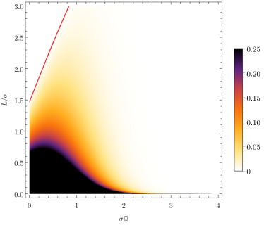
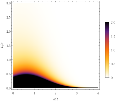
if and only if . Using the expressions in Eqs. (50) and (51), we plot the concurrence of the state in Fig. 1a.
For a system of two qubits, the concurrence can be used to calculate the entanglement of formation , defined as the number of the maximally entangled states needed to prepare Bruß and Leuchs (2007); *Nielsen:2010
| (60) |
where . From the above we see that in the standard units of a bipartite entanglement, the so called ebit, the entanglement between the two detectors in a perturbative regime is relatively week: it scales as .
Neither of these quantities is accessible by local measurements of either detector. Instead, we consider two local observers, one in possession of detector and the other in possession of detector , each measuring the observable Pauli operator , and quantify the correlation in the outcomes of their measurements. We characterize their results by random variables and , respectively, with . The correlation between these variables is given by
| (61) |
where is the covariance between and and and are the variances associated with and . In Minkowski space, when the switching function of the two detectors is coincident, the correlation between the measurements performed on the two detectors is given by
| (62) |
III Detectors in quotients of Minkowski space
We now consider an analogous situation in two different quotient spacetimes of Minkowski space with non-trivial spatial topologies. The first is a cylindrical universe
| (63) |
which is constructed as a quotient of Minkowski space with the group generated by the discrete isometry .
The second spacetime we consider , is again a cylindrical universe in which rotations by in the -plane have been identified
| (64) |
where the group is generated by the discrete isometry .
The compactification scale of these two spacetimes is . Both and preserve space and time orientation and act freely and properly 111Let be a group which acts on a topological space . A group action is said to act freely if for all , implies is the identity. A group action is said to act properly if the map is proper, that is inverses of compact sets are compact., this ensures that both and are space and time orientable Lorentzian manifolds. As neither and affect the Minkowski line element, both and are locally flat spacetimes. The behaviour of particle detectors in both of these spacetimes has been studied in the past, with a focus on applications to Hawking radiation and the Unruh effect Louko and Marolf (1998); Langlois (2005).
The advantage of considering spacetime topologies built from quotients of Minkowski space, is that the Wightman function in the quotient spacetimes can be easily constructed via the method of images from the Wightman function in Minkowski space. If we are given a Green’s function on a spacetime , we can construct the corresponding Green’s function on the quotient spacetime by the image sum Banach and Dowker (1979a); *Banach:1979a
| (65) |
where denotes the group action of the group element on and corresponding to normal scalar fields and twisted fields respectively. From now on we will restrict ourselves to for simplicity; the results presented are easily generalizable to twisted fields.
Making use of Eq. (65), along with the Wightman function in Minkowski space, Eq. (49), the Wightman function in both and can be constructed, and used to evaluate the transition probability in Eq. (45), and the matrix elements and in Eqs. (46) and(47) respectively, in both spacetimes. We consider two detectors with the world lines
| (66) |
where and are two dimensional vectors lying in the -plane. Matrix elements of up to the second order in in are given by
| (67) | ||||
| (68) | ||||
| (69) |
where and ; while in these quantities are given by Eqs. (67)-(69), with the substitutions
| (70) | ||||
| (71) |
where with and is zero or one for even and odd respectively.
Note that , , and for detectors in depend on the absolute position of the two detectors, as can be seen from the dependence of Eqs. (70) and (71) on and . This is a qualitative difference between , and both the cylindrical universe and Minkowski space , stemming from the fact that is not translationally invariant in the -plane, which can bee seen from the isometry used to define . Consequently, , as defined in Eq. (42), which was true for both and , and Eq. (61) must be used to calculate the correlation function.
From the Eqs. (67)–(69) we see for a large compactification scale of the quotient spacetimes, i.e., , the contribution to the transition probability and exchange probability from the image sums vanish, resulting in and . Consequently, in this limit the two universes are indistinguishable by measurements of either the transition probability of a single detector or the resulting entanglement between two detectors.
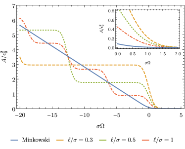
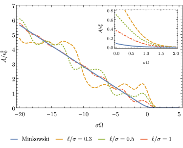
To examine the effect the spatial topology of a spacetime has on the transition probability of a detector, in Fig. 2 we plot the transition probabilities , , and , in Minkowski space , the cylindrical spacetime , and the spacetime . The oscillations in the cases of and are expected and akin to the appearance of modified quasi-normal modes in spacetimes with closed topologies (see, for instance Ng et al. (2014)).
The dependence of the transition rate, that is the derivative of the transition probability, on spatial topology for detectors that have been on for an infinite amount of time in both and has been studied in Langlois (2005). In black hole spacetimes with identical geometry but differing spatial topology, the transition rate of detectors has been studied in Smith and Mann (2014).
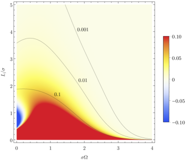
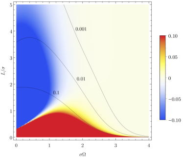
In examining the effect the spatial topology has on vacuum entanglement, we plot in Fig. 3 the difference in correlations functions between detectors in and and detectors in and .
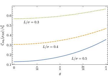
In both and the concurrence of the joint state of the two detectors depends on the orientation of the detectors with respect to the identified direction. Thus, in principle, by measuring vacuum corrections one may infer a preferred direction induced by the spatial topology of the universe. To illustrate this point, in Fig. 4 we plot the dependence of the concurrence of on the orientation of the two detectors in the spacetime with respect to the identified direction.
For the purposes of plotting, in Figs. 1-4, we truncate the image sums at , as the inclusion of more terms does not affect the plots. This is because the contribution from larger terms in the image sums decease quickly as grows: , which can be seen from Eqs. (67)-(69).
IV Discussion and outlook
In the spacetimes we analyzed ( and ), the effects of global structure show up as small deviations in transition rate of a single particle detector, and entanglement and observable correlations between two detectors from their counterparts in the spatially Euclidean Minkowski spacetime. However, in the limit of zero extrinsic curvature, i.e. when the compactification scale becomes infinite, these deviations approach zero and the results coincide with that of Minkowski space. We plan to disentangle the role of extrinsic curvature from that of entirely topological effects in future work.
The Minkowskian result is recovered in the limit . Since in cosmological scenarios we expect the topological scale to be at the order of the Hubble scale, and the effective experimental run-time is at the order of years at best, we expect , making the effects unobservable. By the same token we expect that entanglement between different degrees of freedom during early Universe, where the relevant dimensionless ratios were of order of 1 or higher, to be significantly impacted by the emerging global structures. We plan to investigate these effects in future work.
On the other hand, although the discussion throughout this paper has focused on the spatial topology of the entire Universe, the tools used and results presented apply equally well to fields and detectors in cavities with appropriate boundary conditions. Specifically, the results given regarding the cylindrical universe are equivalent to detectors and the field in a cavity with periodic boundary conditions. Further, the blue regions in Fig. 3 suggest that entanglement harvesting from a quantum field may be increased by constructing cavities with appropriate boundary conditions. In fact, there is already substantial evidence that this is the case: Entanglement harvesting in cavities has already been analyzed non-perturbatively in Brown et al. (2013) and further in Martín-Martínez et al. (2013b), where it was shown that a combination of harvesting in cavity setups complemented with communication yields a sustainable source of quantum entanglement. This particular amplification of harvesting in cavity setups is otherwise impossible in free space.
A different group of questions deals with entanglement and correlations between the detectors in relative motion Peres and Terno (2004), as well as with the effects of delay between switching the detectors. Finally, it is interesting to investigate the build-up of the correlations between the detectors in time.
The density matrix of Eq. (40) has the same form at all orders of perturbation theory. Nevertheless, it will be instructive to obtain non-perturbative results that are based on non-perturbative methods following the several different formalisms developed for harmonic oscillator detectors Lin and Hu (2006); Brown et al. (2013); Bruschi et al. (2013), as well is to compare different types of detectors.
Acknowledgements.
The authors would like to thank Nicolas C. Menicucci and Robert B. Mann for useful discussions.Appendix A State of the detectors and entanglement measures
A.1 Calculation of
Here we provide the details of the perturbative calculations that lead to the reduced density matrix in Eq. (42). We present the derivation in Minkowski space, but it translates verbatim to any stationary spacetime.
Here we work in the Scrödinger picture as it will be more convenient than the interaction picture to extract the structure of the reduced density matrix to all orders in perturbation theory. The Hamiltonian describing two detectors interacting with the scalar field is given by
| (72) |
where and are the free Hamiltonians of detectors and with energy gaps and , is the free Hamiltonian of the scalar field, and is the interaction Hamiltonian in the Schördinger picture
| (73) |
where the subscript reminds us that we are working in the Scrödinger picture. We choose the switching functions and to be proportional to our perturbation parameter ; in the analysis presented we took , but in general other switching functions may be studied. Since both detectors are inertial and at rest with respect to one another, we have equated the proper time of each detector with the coordinate time .
Initially () the detectors are in their ground state and the field in the vacuum state
| (74) |
We expand the state of the combined system in the eigenstates of the unperturbed Hamiltonian at time as
| (83) |
where labels the energy levels of the detectors with energies and , the index represents a decomposition over the basis states of the scalar field, and where . The coefficients satisfy the Schrödinger equation
| (92) | ||||
| (101) |
where is the Pauli matrix. We represent the coefficients in a more explicit form as
| (102) |
i.e., spell out explicitly the vacuum, one-particle, two-particle, etc. components. To simplify the notation we label the terms as and as , and suppress the arguments. Contributions of these elements to the inner product that is performed with the appropriate measure will be denoted in the usual vector form, such as or .
The solution to Eq. (101), subject to the initial condition given in Eq. Eq. (74), is given schematically as
| (103) | |||
| (104) | |||
| (105) | |||
| (106) |
As a result, the non-zero matrix elements of the reduced density matrix in Eq. (40) describing the joint state of the two detectors, up to the fourth order in are given by
| (107) | |||
| (108) | |||
| (109) | |||
| (110) | |||
| (111) | |||
| (112) |
By construction is normalized.
To calculate the transition probability, correlations, and measures of entanglement in the leading order, we need the coefficients up to order :
| (113) | |||
| (114) | |||
| (115) | |||
| (116) |
where in the second order coefficients the index stands either for vacuum (0) or a two-particle state (). , , and
The matrix elements of are obtained from Eqs. (113)-(116) with the help of Eq. (39). For identical detectors the matrix elements , , and are obtained straight forwardly from Eqs. (113)–(116), and result in the quantities , , and respectively, and are given in Eqs. (45)–(47).
As for the matrix element , applying Eq. (39) results in
| (117) |
The four 4-point functions appearing in Eq. (117) can be expanded in terms of products of Wightman functions using the commutation properties of the field, yielding
| (118) |
where we have exploited the fact that the detectors are at rest with respect to one another, which results in .
The first term appearing in Eq. (118) is immediately identified as , where is given in Eq. (46). By changing the integration variables to
| (119) |
and then to
| (120) |
the second and third terms in Eq. (118) result in and respectively, where and are defined in Eq. (45) and in Eq. (47). Thus we find
| (121) |
The matrix element is obtained either directly from its definition or by exploiting the normalization condition .
A.2 Quantifying the entanglement in
We give here negativity and concurrence for the density matrix of (40). In the case
| (122) |
and
| (123) |
which simplifies further if to
| (124) |
If then
| (125) |
and
| (126) |
In a general two-qubit system concurrence and negativity are related by Verstraete et al. (2001)
| (127) |
The negativity is equal to the concurrence if the eigenvector of the partially transposed state corresponding to its negative eigenvalue is one of the Bell states (up to local unitary transformations). Indeed, for the identical detectors () when the two quantities coincide and the eigenvector in question becomes .
Appendix B The Wightman function
To ease comparison between different sources, we first spell out how our convention for the Wightman function relates to the definitions in other references we use. In particular,
| (128) |
where is introduced in Birrell and Davies (1982) (and is called in the massless case), is introduced in Bogoliubov and Shirkov (1980), and is called in Scharf (1989).
Wightman functions are well-defined distributions, i.e. they can be represented as a distributional limit of regular analytic functions Bogoliubov and Shirkov (1980). However, representation in terms of functions that are also covariant requires a regularization procedure, e.g., the Pauli-Villars regularization. A simple popular representation uses the “” prescription Birrell and Davies (1982)
| (129) |
Eq. (129) is not manifestly covariant, and requires additional manipulations to obtain, for example, the Unruh effect Schlicht (2004). On the other hand, a straightforward calculation demonstrates that the distributional form of the Wightman function as given by Eq. (49) is free from these complications.
For convenience, we summarize here several properties of distributions that we employed in obtaining Eqs. (50) and (51) Bogolubov et al. (1990). Recall that the definition of a distribution acting on a test function is given by
| (130) |
where the function defines the distribution . The derivative of a distribution is obtained from the above definition by integrating by parts to give
| (131) |
The distribution acting on a test function is defined as
| (132) |
where denotes that the principle value of the integral should be taken. All the subsequent inverse power distributions are defined as distributional derivatives of , hence
| (133) |
Eq. (133) is used in arriving at the expression for given in (51).
Particular care is required for the evaluation of integrals involving the delta-function term of the Wightman function when . We consider the distribution as a limit of
| (134) |
This prescription results in the action of the distribution on a test function to be
| (135) |
Eq. (135) is used in arriving at the expression for given in (50).
References
- Hawking and Ellis (1973) S. W. Hawking and G. F. R. Ellis, The large scale structure of space-time (Cambridge University Press, 1973).
- Thiemann (2008) T. Thiemann, Modern canonical quantum general relativity (Cambridge University Press, 2008).
- Engle (2014) J. Engle, in “Springer Handbook of Spacetime”, edited by A. Ashtekhar and V. Petkov (Springer, 2014) Chap. Spin Foams, p. 783.
- Martin et al. (2014) J. Martin, C. Ringeval, and V. Vennin, Phys. Dark Univ. 5-6, 75 (2014).
- Ade et al. (2014a) P. Ade et al. (Planck), Astron. Astrophys. 571, A26 (2014a).
- Ade et al. (2014b) P. Ade et al. (Planck), Astron. Astrophys. 571, A25 (2014b).
- Peres and Terno (2004) A. Peres and D. R. Terno, Rev. Mod. Phys. 76, 93 (2004).
- Bruß and Leuchs (2007) D. Bruß and G. Leuchs, Lectures on Quantum Information (Wiley-VCH, 2007).
- Nielsen and Chuang (2010) M. A. Nielsen and I. L. Chuang, Quantum Computation and Quantum Information (Cambridge University Press, 2010).
- Davies (1975) P. C. W. Davies, J. Phys. A: Gen. Phys. 8, 609 (1975).
- Fulling (1973) S. A. Fulling, Phys. Rev. D 7, 2850 (1973).
- Unruh (1976) W. G. Unruh, Phys. Rev. D 14, 870 (1976).
- Summers and Werner (1985) S. J. Summers and R. Werner, Phys. Lett. A 110, 257 (1985).
- Summers and Werner (1987) S. J. Summers and R. Werner, J. Math. Phys. 28, 2440 (1987).
- Valentini (1991) A. Valentini, Phys. Lett. A 153, 321 (1991).
- Reznik (2003) B. Reznik, Found. Phys. 33, 167 (2003).
- Hu et al. (2012) B. Hu, S.-Y. Lin, and J. Louko, Class. Quant. Grav. 29, 224005 (2012).
- Pozas-Kerstjens and Martín-Martínez (2015) A. Pozas-Kerstjens and E. Martín-Martínez, (2015), arXiv:1506.03081 .
- Salton et al. (2015) G. Salton, R. B. Mann, and N. C. Menicucci, New J. Phys. 17, 035001 (2015).
- Ver Steeg and Menicucci (2009) G. Ver Steeg and N. C. Menicucci, Phys. Rev. D 79, 044027 (2009).
- DeWitt (1979) B. S. DeWitt, “in General Relativity: an Einstein Centenary Survey”, edited by S. W. Hawking and W. Israel (Cambridge University Press, 1979) Chap. Quantum Gravity: the New Synthesis, p. 680.
- Crispino (2008) L. C. B. Crispino, Rev. Mod. Phys. 80, 787 (2008).
- Martín-Martínez et al. (2013a) E. Martín-Martínez, M. Montero, and M. del Rey, Phys. Rev. D 87, 064038 (2013a).
- Alhambra et al. (2014) A. M. Alhambra, A. Kempf, and E. Martín-Martínez, Phys. Rev. A 89, 033835 (2014).
- Ali et al. (2010) M. Ali, A. R. P. Rau, and G. Alber, Phys. Rev. A 81, 042105 (2010).
- Bogoliubov and Shirkov (1980) N. N. Bogoliubov and D. V. Shirkov, Introduction to the Theory of Quantized Fields (John Willey & Sons, 1980).
- Bogolubov et al. (1990) N. N. Bogolubov, A. A. Logunov, A. I. Oksak, and I. T. Todorov, General Principles of Quantum Field Theory (Springer, 1990).
- Scharf (1989) G. Scharf, Finite Quantum Electrodynamics (Springer, 1989).
- Birrell and Davies (1982) N. D. Birrell and P. C. W. Davies, Quantum fields in curved space (Cambridge University Press, 1982).
- Martin-Martinez and Menicucci (2012) E. Martin-Martinez and N. C. Menicucci, Class. Quant. Grav. 29, 224003 (2012).
- Wootters (1998) W. K. Wootters, Phys. Rev. Lett. 80, 2245 (1998).
- Louko and Marolf (1998) J. Louko and D. Marolf, Phys. Rev. D 58, 024007 (1998).
- Langlois (2005) P. Langlois, Imprints of Spacetime Topology in the Hawking-Unruh Effect, Ph.D. thesis, University of Nottingham (2005), arXiv:gr-qc/0510127 .
- Banach and Dowker (1979a) R. Banach and J. S. Dowker, J Phys. A-Math Theor. 12, 2545 (1979a).
- Banach and Dowker (1979b) R. Banach and J. S. Dowker, J Phys. A-Math Theor. 12, 2527 (1979b).
- Ng et al. (2014) K. K. Ng, L. Hodgkinson, J. Louko, R. B. Mann, and E. Martín-Martínez, Phys. Rev. D 90, 064003 (2014).
- Smith and Mann (2014) A. R. H. Smith and R. B. Mann, Class. Quant. Grav. 31, 082001 (2014).
- Brown et al. (2013) E. G. Brown, E. Martín-Martínez, N. C. Menicucci, and R. B. Mann, Phys. Rev. D 87, 084062 (2013).
- Martín-Martínez et al. (2013b) E. Martín-Martínez, E. G. Brown, W. Donnelly, and A. Kempf, Phys. Rev. A 88, 052310 (2013b).
- Lin and Hu (2006) S. Lin and B. L. Hu, Phys. Rev. D 73, 124018 (2006).
- Bruschi et al. (2013) D. E. Bruschi, A. R. Lee, and I. Fuentes, J. Phys. A: Math. Theor. 46, 165303 (2013).
- Verstraete et al. (2001) F. Verstraete, K. Audenaert, J. Dehaene, and B. D. Moor, J. Phys. A: Gen. Phys. 34, 10327 (2001).
- Schlicht (2004) S. Schlicht, Class. Quant. Grav. 21, 4647 (2004).