TAPAS - Tracking Advanced Planetary Systems with HARPS-N.

Abstract

Context. Lithium rich giant stars are rare objects. For some of them, Li enrichment exceeds abundance of this element found in solar system meteorites, suggesting that these stars have gone through a Li enhancement process.

Aims. We identified a Li rich giant HD 107028 with $\hbox{$\thinspace A(\mathrm{Li})$}>3.3$ in a sample of evolved stars observed within the PennState Toruń Planet Search. In this work we study different enhancement scenarios and we try to identify the one responsible for Li enrichment for HD 107028.

Methods. We collected high resolution spectra with three different instruments, covering different spectral ranges. We determine stellar parameters and abundances of selected elements with both equivalent width measurements and analysis, and spectral synthesis. We also collected multi epoch high precision radial velocities in an attempt to detect a companion.

Results. Collected data show that HD 107028 is a star at the base of Red Giant Branch. Except for high Li abundance, we have not identified any other anomalies in its chemical composition, and there is no indication of a low mass or stellar companion. We exclude Li production at the Luminosity Function Bump on RGB, as the effective temperature and luminosity suggest that the evolutionary state is much earlier than RGB Bump. We also cannot confirm the Li enhancement by contamination, as we do not observe any anomalies that are associated with this scenario.

Conclusions. After evaluating various scenarios of Li enhancement we conclude that the Li-overabundance of HD 107028 originates from Main Sequence evolution, and may be caused by diffusion process.

1 Introduction

Lithium depletion is a natural prediction of stellar evolution. Not long after stars leave Main Sequence they experience mixing, called First Dredge Up (FDU) that will lower the surface abundance levels to values of $\hbox{$\thinspace A(\mathrm{Li})$}=1.5$ dex or less. However, about a hundred Li-rich stars ($\hbox{$\thinspace A(\mathrm{Li})$}>1.5$) among Red Giant (RG) stars have recently been found (Kumar et al. 2011 and references therein, Ruchti et al. 2011; Lebzelter et al. 2012; Martell & Shetrone 2013; Liu et al. 2014; Adamów et al. 2014).

Lithium enhancement via internal production on Red Giant Branch (RGB) can start at the earliest with Luminosity Function Bump (LFB), shortly after FDU ends. LFB is a stage in RGB evolution for stars no more massive than $\approx 2.2\hbox{$\thinspace M_{\odot}$}$. It is associated with the removal of the molecular discontinuity that stems from FDU processes. During LFB, star takes a small ”step-back” in its evolution on the HR diagram - effective temperature increases, while luminosity decreases for a short time, and stellar interior becomes turbulent (Eggleton et al. 2006). Lithium may be produced during that evolutionary phase via a Cameron-Fowler mechanism (Cameron & Fowler 1971) with the support of an extra-mixing mechanism. Cameron-Fowler mechanism is probably responsible for Li production in stars on Asymptotic Giant Branch (AGB). In this case, the thermal pulses can trigger the non-convective mixing.

As additional mixing on RGB begins at the LFB, and the so-called Li-flash is also believed to be associated with this phase (Charbonnel & Balachandran 2000; Pasquini et al. 2014). Thus, attempts to locate the Li-rich stars in the the HR diagram have driven a number of studies trying to verify this Li-production mechanism (e.g., Brown et al. 1989; Pilachowski et al. 1988, 2000; Kumar et al. 2011; Ruchti et al. 2011; Lebzelter et al. 2012; Martell & Shetrone 2013). However, these studies have shown, that Li-rich stars can be found at different stages along the RGB evolution. What is even more interesting, one of the most Li rich star, SDSS J0720+3036 with $\hbox{$\thinspace A(\mathrm{Li})$}=4.55\pm 0.20$ (Martell & Shetrone 2013) was identified to be a subgiant.

All the above have led to proposals of a number of alternative mechanisms invoking the presence of an extra-mixing process or pollution scenarios to explain the high photospheric values. Thus, it has been argued that lithium could be enhanced as a consequence of the stellar readjustments following the accretion of substellar bodies (Alexander 1967; Siess & Livio 1999) or via the accretion of dense interstellar medium clouds which chemical composition was altered by a nearby supernova explosions (Woosley & Weaver 1995). Lithium can also be externally delivered by a companion in a binary system if one of the components has already undergone lithium production on the AGB (Sackmann & Boothroyd 1999). All the scenarios based on external contamination, involve anomalies in chemical abundances other than Li, such as enhancement of neutron capture elements, that are produced via s-process in evolved stars, or $\alpha$ and r-process elements, associated with supernovae (i.e. Terasawa et al. 2001). The accretion of substellar bodies should also increase stellar rotation (Carlberg et al. 2010, 2012) and may cause intense mass loss (de La Reza et al. 1997) The latest searches for planets around giants have provided an opportunity to study the possible connection between lithium abundance and hosting companions of different masses. A planetary companion was found to the Li-rich red giant BD+48 740 Adamów et al. (2012) and in a recent study done for a sample of giants observed within the PennState - Toruń Planet Search (PTPS) project, it is found that Li overabundance is in many cases associated with a presence of companions (Adamów et al. 2014).

All scenarios of Li enhancement on RGB can potentially explain moderate Li overabundances ($\hbox{$\thinspace A(\mathrm{Li})$}\lesssim 2.5$), but do not explain the existence of extremely lithium rich stars. About a hundred of lithium-rich giants have been discover so far. About 14 of there are so-called super lithium-rich giant stars (Brown et al. 1989; Balachandran et al. 2000; Reddy & Lambert 2005; Carlberg et al. 2010; Kumar et al. 2011; Ruchti et al. 2011; Martell & Shetrone 2013; Monaco et al. 2014). These evolved stars have abundances exceeding the interstellar medium value, i.e. $\hbox{$\thinspace A(\mathrm{Li})$}=3.3$ (Asplund et al. 2009).

In this paper we report a chemical abundance analysis of the Li-rich giant star HD 107028. We found the star to have a $\thinspace A(\mathrm{Li})$ exceeding the value of 3.3 determined for meteorites. HD 107028 has been as well the subject of a systematic search for a substellar companion using HARPS-N at the 3.6 m Telescopio Nazionale Galileo under our program TAPAS (Tracking Advanced Planetary Systems with HARPS-N) after it was shown that HET observations show radial velocity (RV) variation of $36\text{\,}\mathrm{m}\,\mathrm{s}^{-1}$, significantly larger than expected stellar jitter.

The paper is organized as follows: in Section 2 we present the observations obtained for this target and we outline the reduction procedures; Section 3 presents stellar parameters; In Section 4 we present abundances determinations; Analysis of available RVs is discussed in Section 5; Section 6 presents data on mass loss and activity; and finally Section 7, which includes the discussion and conclusions, closes the paper.

2 Observations and data reduction.

Table 1: Spectroscopic material used in this work.

Instrument	range	resolution	S/N	date
HET/HRS	4076 – $7838\text{\,}\mathrm{\SIUnitSymbolAngstrom}$	60 000	320 at $5936\text{\,}\mathrm{\SIUnitSymbolAngstrom}$	14 May 2006
HET/HRS	7109 – $10\,917\text{\,}\mathrm{\SIUnitSymbolAngstrom}$	60 000	171 at $8991\text{\,}\mathrm{\SIUnitSymbolAngstrom}$	03 Mar 2013
TNG/HARPS-N	3830 – $6930\text{\,}\mathrm{\SIUnitSymbolAngstrom}$	115 000	141 at $6582\text{\,}\mathrm{\SIUnitSymbolAngstrom}$	28 Apr 2013
Mercator/Hermes	3770 – $9000\text{\,}\mathrm{\SIUnitSymbolAngstrom}$	85 000	178 at $7124\text{\,}\mathrm{\SIUnitSymbolAngstrom}$	22 Jan 2015

HD 107028 (BD+69 657, HIP 59975) is a $V=7.66$, $B-V=+0.84$ and $U-B=+0.45$ (Mermilliod 1986) G5 (Cannon & Pickering 1993) giant in Draco. New reduction of Hipparcos parallaxes delivers $\pi=6.15\pm 0.49$ and places the star at a distance of 163 pc (van Leeuwen 2007). 157 epochs of Hipparcos photometry reveal constant light of H_p=7.8035 $\pm$ 0.0013 mag with a scatter of 0.015 mag. The star belongs to sample of evolved stars observed within the PTPS project. Because of its strong Li lines and the RV variations that could not be resolved with HET precision, it was selected for TAPAS project.

The spectroscopic observations presented in this paper were made with three instruments (see Table 1).The observation started with the 9.2 m effective aperture Hobby-Eberly Telescope (HET, Ramsey et al. 1998) and its High Resolution Spectrograph (HRS, Tull 1998) in the queue scheduled mode (Shetrone et al. 2007). We also observed HD 107028 with the 3.58 m Telescopio Nazionale Galileo (TNG) and its High Accuracy Radial Velocity Planet Searcher in the North hemisphere (HARPS-N, Cosentino et al. 2012) and with 1.2 m Mercator telescope and Hermes spectrograph (Raskin et al. 2011). The instrumental set-ups, reduction and radial velocity measurements for HET/HRS and TNG/HARPS-N were described in detail in Niedzielski et al. (2015) (hereafter Paper 1). We obtained altogether sixteen HET/HRS spectra with typical signal-to-noise ratio (S/N) of 150-200 and 22 TNG/HARPS-N spectra with S/N of 30-100. We also obtained one HET/HRS spectrum made in a different than standard PTPS spectrograph configuration. This spectrum covers more red wavelength region and includes CN lines at $\lambda$8003\text{\,}\mathrm{\SIUnitSymbolAngstrom}$$. We used standard IRAF scripts or HET/HRS data reduction. Data reduction for Mercator/Hermes spectrum was done using the automated pipeline.

3 Stellar parameters

For abundance analysis we used the four most suitable spectra available to us: two blue ones, with the highest S/N, one from TNG/HARPS-N and the other from HRS/HRS (only in GC0 mode); and two red ones, HET/HRS spectrum that covers $\lambda$8000\text{\,}\mathrm{\SIUnitSymbolAngstrom}$$ region and one Mercator/Hermes spectrum.

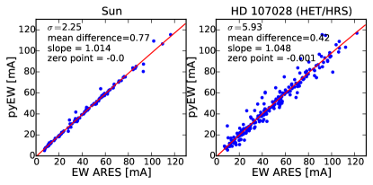
Figure 1: Comparison of equivalent widths determined with ARES and pyEW for the Sun and HD 107028.

The first estimate of stellar parameters was done using the available photometric data. For this purpose we used BVJHK magnitudes from TYCHO and 2MASS catalogs and $\thinspace T_{\mathrm{eff}}$ - color calibrations from Ramírez & Meléndez (2005). From this analysis, the effective temperature of HD 107028 was estimated as 5100 K but no reliable $\log g$ was available. The luminosity of HD 107028 was calculated from the Hipparcos parallax (van Leeuwen 2007). The effective temperatures agree within uncertainties.

To constrain the atmospheric parameters, mass and luminosity of HD 107028 as well as possible, we repeated the analysis with new spectra and a new method. For this purpose, we developed a set of Python functions to measure equivalent widths (EWs) of Fe I and Fe II lines and to evaluate stellar parameters using the current version of the MOOG stellar line analysis code (Sneden 1973).

The pyEW Python procedures for determination of EWs is based on ideas used in the ARES code (Sousa et al. 2007). It redetermines continuum in a small portion of the spectrum (usually $2\text{\,}\mathrm{\SIUnitSymbolAngstrom}$), calculates derivatives to detect positions of lines and fits multiple gaussian profiles to the observed spectrum. In Figure 1 we present the comparison of equivalent widths determined with pyEW and ARES for Sun (100 lines) using solar HARPS spectrum distributed with ARES code, and for HD 107028 (208 lines). For the latter we used the HET/HRS spectrum. In both cases we obtained very good agreement, although the scatter, as expected, is higher for the HET/HRS spectrum given its lower S/N and resolution compared to the solar spectrum.

Table 2: Summary of parameters for HD 107028 and Sun.

Fe lines by Takeda
Parameter	HET/HRS	HERMES	HARPS-N	Sun
$\thinspace T_{\mathrm{eff}}$	$5124\pm 41$	$5109\pm 38$	$5104\pm 39$	$5790\pm 47$
$\log g$	$2.97\pm 0.06$	$3.01\pm 0.06$	$3.0\pm 0.06$	$4.44\pm 0.06$
$\thinspace v_{\mathrm{mic}}$	$1.05\pm 0.06$	$1.11\pm 0.05$	$1.03\pm 0.06$	$0.97\pm 0.06$
$[$Fe/H$]$	$-0.25\pm 0.06$	$-0.30\pm 0.05$	$-0.26\pm 0.06$	$-0.09\pm 0.06$
EP slope	0.00238	0.00706	-0.00308	-0.01773
RW slope	0.00121	-0.00465	-0.04525	0.02918
$n_{\mathrm{FeI}}$	194	227	193	173
$n_{\mathrm{FeII}}$	15	18	14	14
a compilation of Fe and Ti lines with laboratory data
Parameter	HET/HRS	HERMES	HARPS-N	Sun
$\thinspace T_{\mathrm{eff}}$	$5190\pm 70$	$5139\pm 67$	$5132\pm 64$	$5833\pm 63$
$\log g$	$2.96\pm 0.11$	$2.94\pm 0.11$	$2.94\pm 0.11$	$4.37\pm 0.13$
$\thinspace v_{\mathrm{mic}}$	$1.19\pm 0.10$	$1.07\pm 0.09$	$1.04\pm 0.09$	$0.96\pm 0.08$
$[$Fe/H$]$	$-0.32\pm 0.10$	$-0.31\pm 0.10$	$-0.23\pm 0.09$	$-0.03\pm 0.08$
EP slope	0.01685	-0.00414	0.00675	-0.00641
RW slope	-0.025578	-0.00981	-0.02349	0.02659
$n_{\mathrm{FeI}}$	78	103	96	96
$n_{\mathrm{FeII}}$	33	38	31	33

The analysis was done using three different spectra (the red HET/HRS was not included in analysis) and two line sets. The first set of Fe I and II lines is adopted from Takeda et al. (2005), who calibrated line data on the solar spectrum. The second set of neutral and ionized Fe and Ti features is a compilation of lines for which $\log gf$ are determined in laboratory studies. The $\log gf$ values for Fe I are taken from Den Hartog et al. (2014); Ruffoni et al. (2014) and O’Brian et al. (1991); Fe II lines are from Meléndez & Barbuy (2009). We also added Ti I and Ti II lines with $\log gf$ values taken from Lawler et al. (2013) and Wood et al. (2013), respectively. obtained by the University of Wisconsin atomic physics group. From this compilation we chose isolated and moderately blended lines that are present in our spectra. For the analysis we used only lines with equivalent widths in the $$5\text{\,}\mathrm{m\SIUnitSymbolAngstrom}$<\mathrm{EW}<$150\text{\,}\mathrm{m\SIUnitSymbolAngstrom}$$ range. We used only lines with $\lambda>$4350\text{\,}\mathrm{\SIUnitSymbolAngstrom}$$ due to the low S/N on the blue end of all spectra of HD 107028.

In determining atmospheric parameters we used MOOG’s abfind driver executed from a python wrapper that iterates input stellar parameters and evaluates MOOG results. Iteration is made in the ($\hbox{$\thinspace T_{\mathrm{eff}}$},\log g,\hbox{$\thinspace v_{\mathrm{mic}}$}$) space with the kMPFIT algorithm (a Python implementation of the Levenberg-Marquardt technique to solve the least-squares problem) which is a part of the Kapteyn package. Adopted starting parameters are: $\hbox{$\thinspace T_{\mathrm{eff}}$}=5100$ (obtained form photometric data), $\log g=3.0$, $\hbox{$\thinspace v_{\mathrm{mic}}$}=1.0$ and [Fe/H]=0.0. For the calculations, we used a grid of atmospheres by Castelli & Kurucz (2004). For a given set of $\hbox{$\thinspace T_{\mathrm{eff}}$},\log g,\hbox{$\thinspace v_{\mathrm{mic}}$}$ and [Fe/H], we update the atmosphere model using a tool by Andy McWilliam and Inese Ivans for interpolating between grids. During every iteration, all abundances for single Fe I and Fe II lines that differ from the average Fe I and Fe II values (respectively) by more than $1\sigma$ are removed from the fit. This criterion might be considered too strict, but initial $\sigma$ is calculated for all abundances from all automatically measured lines. Usually, there are some faulty EWs measurements among them that need to be removed from further analysis. In case of HD 107028, $1\sigma$ threshold means eliminating all values for which the difference between single abundance and average abundance is greater than 0.5 dex. Input file where lines and their EWs are listed, is not edited, therefore this procedure is repeated for every iteration.

The results obtained for different line lists and stellar spectra are summarized in Table 2. Uncertainties presented there are estimated in a way proposed by Gonzalez & Vanture (1998). The uncertainties in $\thinspace T_{\mathrm{eff}}$ and $\thinspace v_{\mathrm{mic}}$ were estimated based on parameters of abundances versus excitation potential and reduced EWs fits (respectively) for the best model. Uncertainty in $\log g$ is a quadrature sum of the uncertainty in $\thinspace T_{\mathrm{eff}}$ and the scatter in Fe II abundances, and for uncertainty in [Fe/H] is a quadrature sum of the uncertainties in $\hbox{$\thinspace T_{\mathrm{eff}}$},\log g,\hbox{$\thinspace v_{\mathrm{mic}}$}$ and the scatter in Fe I abundances.

The final parameters adopted for further analysis are: $\hbox{$\thinspace T_{\mathrm{eff}}$}=5133\pm 53$ K, $\log g=2.97\pm 0.09$, $\hbox{$\thinspace v_{\mathrm{mic}}$}=1.08\pm 0.08\hbox{$\thinspace{\mathrm{km\leavevmode\nobreak\ s^{-1}}}$}$ and [Fe/H]$=-0.28\pm 0.08$ (averaged values). The effective temperature we obtained is in agreement with the one based on intrinsic colors. These parameters locate unambiguously HD 107028 in the subgiants/giants area in the HR diagram.

The stellar mass and age of HD 1070028 were estimated on the basis of spectroscopically determined atmospheric parameters through construction of a probability distribution function using an estimation by da Silva et al. (2006) and stellar isochrones from PARSEC (PAdova and TRieste Stellar Evolution Code, Bressan et al. 2012). The stellar radius was estimated from the derived masses and log g values obtained from the spectroscopic analysis, and using the derived luminosities and effective temperatures. The adopted radius is the average of the two estimates. The $v_{rot}\sin i_{\star}$ was obtained via SME (Valenti & Piskunov 1996) by modeling a set of spectral lines with a procedure described by Adamów et al. (2014). The stellar parameters of HD 107028 are summarized in Table 3 and its location on the Hertzsprung-Russell diagram is presented in Fig. 2 .

Table 3: Summary of available data on HD 107028.

Parameter	value	reference
V [mag]	7.57	ESA 1997
B-V [mag]	0.84	Mermilliod (1986)
$\pi$[mas]	$6.15\pm 0.49$	van Leeuwen (2007)
(B-V)0 [mag]	0.816
MV [mag]	1.54
$\thinspace T_{\mathrm{eff}}$ [K]	$5133\pm 53$	This work
$\log g$	$2.97\pm 0.09$	This work
$[$Fe/H$]$	$-0.28\pm 0.08$	This work
$\thinspace v_{\mathrm{mic}}$	$1.08\pm 0.08$	This work
RV [kms-1]	-24.985$\pm$0.026	Nowak (2012)
$v_{\mathrm{rot}}\sin i_{\star}$ [$\thinspace{\mathrm{km\leavevmode\nobreak\ s^{-1}}}$]	1.46$\pm$1.19	Adamów (2014)
$M/\hbox{$\thinspace M_{\odot}$}$	1.72$\pm$0.21	This work
$\log L/L_{\odot}$	1.37 $\pm$0.12	This work
$R/\hbox{$\thinspace R_{\odot}$}$	6.6$\pm$1.0	This work
$\log\mathrm{age}$	9.20$\pm$0.14	This work
$V_{\mathrm{osc}}$ [ms-1]	3.01	This work
$P_{\mathrm{osc}}$ [d]	0.07

4 Abundances

Lithium, CNO, neutron capture elements abundances and carbon isotopic ratio analysis was performed with a python code that make use of the MOOG code (synth driver). The use of spectral synthesis technique in obtaining abundances of those elements is motivated by the fact, that their lines are blended with other structures, might be affected by telluric lines or, like in case of C and N, abundance analysis is based on molecular lines. The procedure starts by building an initial synthetic spectrum, that then is cross correlated with the observations to determine possible RV shifts. After that, an automatic abundance analysis is performed, where fitting a requested set of chosen free parameters is executed using the kMPFIT algorithm. Except for abundances, we look for the best value of a parameter that describes gaussian smoothing of synthetic spectrum and we allow for small adjustments of the continuum level. In this iterated procedure, new synthetic spectra with a varying set of abundances is compared to the observed spectra in search for the best fit.

We determined abundances of the $\alpha$ elements using the isolated lines selected by Ramírez & Allende Prieto (2011) from the measurement of their equivalent widths. Our final abundances for HD 107028 are summarized in Table 4.

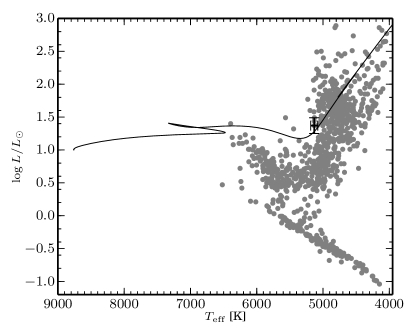
Figure 2: HD 107028 on top of all PTPS stars. Evolutionary track comes from PARSEC and it starts with hydrogen ignition.

4.1 Lithium

The Li I $6708\text{\,}\mathrm{\SIUnitSymbolAngstrom}$ resonance feature is the one of the strongest lines in HD 107028 spectra and proves that this star should be classified as a Li-rich giant (see also Fig. 3 for lithium abundance distribution for evolved stars from PTPS sample).

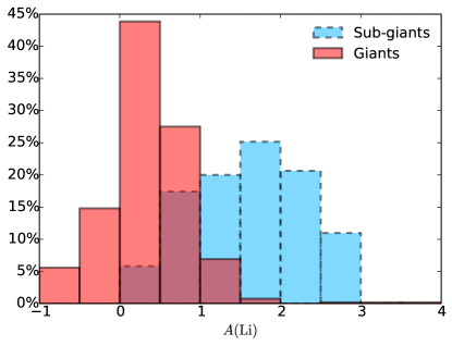
Figure 3: Distribution of Li abundances for evolved stars observed within PTPS (Adamów 2014).

The subordinate $6104\text{\,}\mathrm{\SIUnitSymbolAngstrom}$ line is also detectable in this star, but it is much weaker and located near strong Fe structures. Lithium abundance for HD 107028 was determined using those two lines from TNG/HARPS-N spectrum with the best signal to noise ratio (141 around $6708\text{\,}\mathrm{\SIUnitSymbolAngstrom}$ and 152 close to $6103\text{\,}\mathrm{\SIUnitSymbolAngstrom}$). The obtained values, presented in Table 4, are in agreement, however the abundance based on the stronger, redder line might be underestimated, as the model spectrum does not reach the core of the spectral line (Fig. 4, middle panel). In the case of HD 107028, the imperfect fit of the bottom of the line may be caused by the fact that models might not properly consider the environment where the $6708\text{\,}\mathrm{\SIUnitSymbolAngstrom}$ line is formed. This difference in abundances derived from the two Li lines is also observed for other Li rich giants, i.e. for those discussed in Martell & Shetrone (2013). Lithium lines may be subject to several non-LTE processes (Carlsson et al. 1994 and references therein). We applied the non-LTE corrections provided by Lind et al. (2009) to our LTE lithium abundances, calculated for a star of given $\hbox{$\thinspace T_{\mathrm{eff}}$},\;\log g,\;\hbox{$\thinspace v_{\mathrm{mic}}$}$ and [Fe/H].

The Mercator/Hermes spectrum includes also red Li lines at $8126\text{\,}\mathrm{\SIUnitSymbolAngstrom}$. Those lines are blended with Fe and CN structures and are located in a region of the spectrum that may be affected by H₂O telluric bands. Telluric correction has not been applied to the Mercator/Hermes spectrum, but, based on the plot of the spectrum in Fig. 4 (lower panel) where the best fit of the stellar synthetic spectrum to the observational data is presented, there is no significant telluric contamination close to the Li line that could influence the abundance determination. The obtained value of $\thinspace A(\mathrm{Li})$ of 3.64 is in good agreement with the value determined from the $\lambda$6103\text{\,}\mathrm{\SIUnitSymbolAngstrom}$$ line.

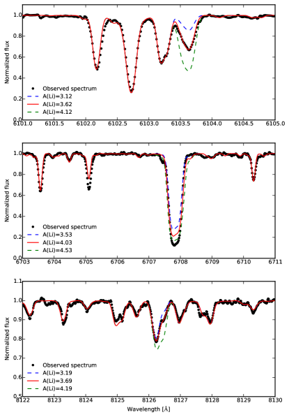
Figure 4: Lithium lines identified in HD 107028 spectrum.

4.2 CNO abundances and carbon isotopic ratio

Oxygen abundance was obtained from the analysis of the lines at $\lambda 6300$, and $6363\text{\,}\mathrm{\SIUnitSymbolAngstrom}$. Since these two lines are not affected by non-LTE effects, no non-LTE correction was applied to determine the oxygen abundance. Both lines lay in a region affected by telluric lines, hence spectral analysis was performed on a spectrum to which telluric division had been applied. The line at $\lambda$6300\text{\,}\mathrm{\SIUnitSymbolAngstrom}$$ is also blended with a Ni line and lies in region where CN bands may influence the analysis.

The oxygen abundance was also obtained from the analysis of the $\lambda$7772, 7774, and $7775\text{\,}\mathrm{\SIUnitSymbolAngstrom}$ triplet, available from HET/HRS and Mercator/Hermes spectra. Since the oxygen triplet is strongly affected by non-LTE effects, we applied the empirical non-LTE corrections by Afşar et al. (2012).

Carbon abundance was determined by modeling of several C₂ (near $5160\text{\,}\mathrm{\SIUnitSymbolAngstrom}$ and $5635\text{\,}\mathrm{\SIUnitSymbolAngstrom}$) and CH bands (4230 - $4240\text{\,}\mathrm{\SIUnitSymbolAngstrom}$ and 4300-$4325\text{\,}\mathrm{\SIUnitSymbolAngstrom}$). The abundance of carbon obtained is [C/H]$=-0.50\pm 0.05$.

The abundance of Nitrogen was determined based on CN bands near $8003\text{\,}\mathrm{\SIUnitSymbolAngstrom}$, using the red HET/HRS spectrum and the Mercator/Hermes spectrum. Although the HET/HRS spectrum has a low signal to noise ratio, the values measured from both spectra are in agreement. Nitrogen, with an abundance of [N/H]=0.6 is enhanced in the HD 107028 atmosphere. However, it is important to keep in mind that the N abundance determined using CN bands strongly depends on the C abundance introduced in the analysis.

The Mercator/Hermes spectrum, that targets CN bands at $8003\text{\,}\mathrm{\SIUnitSymbolAngstrom}$, was used to determine the carbon isotopic ratio. The ¹³C lines are visible but they are not strong, and the obtained $\thinspace{}^{12}\mathrm{C}/^{13}\mathrm{C}$ ratio is 25. The S/N covering the CN bands close to $8003\text{\,}\mathrm{\SIUnitSymbolAngstrom}$ is too low to determine reliable $\thinspace{}^{12}\mathrm{C}/^{13}\mathrm{C}$ carbon isotopic ratio using the HET/HRS spectrum. Therefore, we used, for this purpose, the CH bands near 4230 and $4370\text{\,}\mathrm{\SIUnitSymbolAngstrom}$ and we compared the observational data with a synthetic spectra using MOOG assuming different carbon isotopic ratios. The determinations based on different molecules are in agreement, showing that in HD 107028 the FDU is in progress. Line data for C₂ comes from Ram et al. (2014) and Brooke et al. (2013), CN and CH data were taken from Sneden et al. (2014) and Plez & Cohen (2005), respectively.

Table 4: Summary of abundances on HD 107028. Errors for $A(\mathrm{X})$ are standard deviations and they cover line to line deviations only.

Element	$A(\mathrm{X})_{LTE}\pm\sigma$	$A(\mathrm{X})_{NLTE}$	$A(\mathrm{X})_{\odot}$	$[$X/H$]$	$[$X/Fe$]$
Li${}_{$6104\text{\,}\mathrm{\SIUnitSymbolAngstrom}$}$	3.62	3.73	1.05
Li${}_{$6708\text{\,}\mathrm{\SIUnitSymbolAngstrom}$}$	$4.03$	3.54	1.05
Li${}_{$8126\text{\,}\mathrm{\SIUnitSymbolAngstrom}$}$	3.69		1.05
C	$7.93\pm 0.05$		8.43	-0.50	-0.23
N	8.22		7.83	0.39	0.66
O	$8.47\pm 0.02$		8.69	-0.22	0.05
$\alpha$ elements
Mg	$7.55\pm 0.15$		7.60	-0.05	0.22
Si	$7.36\pm 0.06$		7.51	-0.15	0.12
Ca	$6.20\pm 0.07$		6.34	-0.14	0.13
Ti	$4.75\pm 0.09$		4.95	-0.20	0.07
Neutron-capture elements
Sr II	2.49		2.87	-0.38	-0.11
Ba II	2.12		2.18	-0.06	0.21
La II	$0.74\pm 0.17$		1.10	-0.36	0.17
Eu II	0.34		0.52	-0.18	0.09
Other elements
Na	$6.19\pm 0.05$		6.24	-0.05	0.22
Al	$6.35\pm 0.07$		6.45	-0.10	0.17
Ni	$6.15\pm 0.08$		6.22	-0.07	0.20

4.3 Abundances of $\alpha$-group, neutron capture elements and kinematics

$\alpha$ element abundances were measured using EWs for several Na, Mg, Al, Ca, Ti and Ni lines selected from Ramírez & Allende Prieto (2011) and using their line data. EWs were obtained automatically with pyEW by fitting gaussian profiles to selected lines using the Mercator/HERMES spectrum. Abundances were obtained using MOOG’s abfind driver.

For the determination of abundances of neutron capture elements we used Ba II line at $\lambda$6141\text{\,}\mathrm{\SIUnitSymbolAngstrom}$$, two La II line at $\lambda 6262$ and $6390\text{\,}\mathrm{\SIUnitSymbolAngstrom}$ and one Eu II line at $\lambda$6645\text{\,}\mathrm{\SIUnitSymbolAngstrom}$$. All those lines have complex structures with isotopic and hyperfine splitting, therefore we used spectral synthesis to analyze them. Line data for those transitions were taken from Lawler et al. (2001a) and Lawler et al. (2001b). Strontium abundance was calculated using line at $\lambda$4077.71\text{\,}\mathrm{\SIUnitSymbolAngstrom}$$. All derived abundances for those elements are shown in Table 4 and they are consistent with the abundances of nearby giants of similar metallicity (see i.e. Luck & Heiter 2007 and Afşar et al. 2012).

The overall results of our abundance analysis are presented in Table 4. We find for HD 107028 typical values of a thin-disk, sub-solar metallicity star and to check its consistency we also computed space velocity components ($U,V,W$) following Johnson & Soderblom (1987) but using the J2000 epoch in the coordinates and the transformation matrix, and parallax and proper motions from the Tycho/Hipparcos Catalog (van Leeuwen 2007). We obtain spatial velocities $(U,V,W)=(-87,-59,-51)\hbox{$\thinspace{\mathrm{km\leavevmode\nobreak\ s^{-1}}}$}$ and the distance to the galactic plane $z=0.13$ kpc. Hence, according to the Ibukiyama & Arimoto (2002) criteria, HD 107028 is a member of the galactic thin disk population, This result agrees with the chemical composition of this star, typical for an object from the galactic thin disk.

5 Radial velocities

HD 107028 was observed within PTPS at 15 epochs over 2669 days between MJD=53755.47 and 56425.15. It showed low level RV variations of $36\hbox{$\thinspace{\mathrm{m\leavevmode\nobreak\ s^{-1}}}$}$ with average uncertainty of $6\hbox{$\thinspace{\mathrm{m\leavevmode\nobreak\ s^{-1}}}$}$ (i.e. $6\sigma$). The RV variability was found to be over an order of magnitude larger than the expected amplitude of p-mode oscillations. We observed also bisector (BS) variations of $82\hbox{$\thinspace{\mathrm{m\leavevmode\nobreak\ s^{-1}}}$}$ with an average uncertainty of $16\hbox{$\thinspace{\mathrm{m\leavevmode\nobreak\ s^{-1}}}$}$ and of unclear nature but uncorrelated with the RV (r= -0.03). No periodic signal was found in these data. A cross-correlation analysis of line profiles in the HET/HRS blue CCD GC0 spectrum of HD 107028 (unaffected by I₂ lines) as well as its GC1 spectra (cleaned from I₂ lines in the process of radial velocity measurements, Nowak 2012; Nowak et al. 2013), showed regular shape of cross correlation function and no trace of a companion.

We attempted to resolve this variability with the more precise and stable TNG/HARPS-N instrument given that following i.e. Adamów et al. (2014), Li-overabundance in giants seems to be related to presence of companions. After 21 epochs of observations with TNG/HARPS-N taken over 517 days between MJD=56277.26 and 56795.04 we found RV variations of only $22\hbox{$\thinspace{\mathrm{m\leavevmode\nobreak\ s^{-1}}}$}$ with average uncertainty of $1.2\hbox{$\thinspace{\mathrm{m\leavevmode\nobreak\ s^{-1}}}$}$ and uncorrelated (r=-0.19) BS variations of only $10\hbox{$\thinspace{\mathrm{m\leavevmode\nobreak\ s^{-1}}}$}$. Neither these data alone, nor combined with HET, showed a periodic signal. Our hybrid approach to model the data (see Paper 1 for details) also failed.

With RV measurements only, we cannot definitely exclude that this star hosts a companion, as the orbital inclination of the potential companions may be such that $\sin i\approx 0$. This kind of ”pole on” systems are not detectable for radial velocity searches. However, the low level of observed RV variations, with an amplitude of only $22\hbox{$\thinspace{\mathrm{m\leavevmode\nobreak\ s^{-1}}}$}$, the lack of correlation between RV and BS and regular shape of the cross correlation function suggests better to consider HD 107028 to be a single star. The mean absolute RV of HD 107028 is $-24.485\pm 0.007\hbox{$\thinspace{\mathrm{km\leavevmode\nobreak\ s^{-1}}}$}$.

This radial velocity differs from an earlier measurement ($-29.20\pm 1.2\hbox{$\thinspace{\mathrm{km\leavevmode\nobreak\ s^{-1}}}$}$; Wilson 1953) by $\sim 4.7\hbox{$\thinspace{\mathrm{km\leavevmode\nobreak\ s^{-1}}}$}$. This point cannot be included in RV fitting for several reasons: there is no date and time when this RV measurement was done, the precision of measurements is very different and finally, time separation between Wilson’s and our measurements is more than 60 years. All that leads to unambiguous orbital solutions, but may suggest that HD 107028 has a low mass companion on a highly elliptical, long period orbit.

We cannot definitely exclude the possibility that our observations cover only the flat part of RV curve during one orbital period. However, assuming that the amplitude in RVs should be close to $5\hbox{$\thinspace{\mathrm{km\leavevmode\nobreak\ s^{-1}}}$}$ and that we have observed only flat fragment of RV curve, orbit of companion hosted by HD 107028 should have $e\gtrsim 0.8$ and a very specific orientation in space (longitude of ascending node of $0^{\circ}$ or $180^{\circ}$). In any other cases, a longterm trend in RVs should have been easily detected in TNG/HARPS or HET/HRS data, but we have not observed it.

Therefore, collected observations cannot definitely exclude the hypothesis that HD 107028 hosts a companion on an elliptical orbit and one needs to keep in mind that RV technique effectiveness depends on system orientation in space. However, we claim that the presence of such a companion is unlikely, as we do not see any long term trends in collected RV data. We also argue that radial velocity measurement by Wilson (1953) might be overestimated for HD 107028.

6 Line profile variations: activity and traces of mass-loss

The Ca II H & K line profiles are widely accepted as stellar activity indicators. Both the Ca II H & K lines and the infrared Ca II triplet lines at $8498-$8542\text{\,}\mathrm{\SIUnitSymbolAngstrom}$$ lay outside HET/HRS wavelength range but the Ca II H & K lines are available to us in the TNG HARPS-N spectra and the 8498-$8542\text{\,}\mathrm{\SIUnitSymbolAngstrom}$  range is present in Mercator/Hermes spectrum. Although the S/N in the blue spectrum for this red giant is not high, no trace of reversal, typical for active stars (Eberhard & Schwarzschild 1913) is present, and no obvious chromospheric activity can be demonstrated neither for TNG/HARPS-N nor for Mercator/Hermes spectra. To quantify possible activity-induced line profile variations we calculated the $S^{\mathrm{i}nst}_{\mathrm{H}K}$ index according to the Duncan et al. (1991) prescription for all 21 epochs of HARPS-N observations. The mean value is $S_{\mathrm{i}nst}=0.35\pm 0.02$ which places HD 107028 among moderately active subgiants according to Isaacson & Fischer (2010).

One of the explanations for Li overabundances in evolved stars implies that Li enhancement is associated with mass ejections (in a form of dust) from the star (see e.g. de La Reza et al. 1997; Siess & Livio 1999; Bharat Kumar et al. 2015) that we would see as infrared excesses. To verify whether HD 107028 presents an infrared excess, we queried the WISE (Wright et al. 2010) and 2MASS catalogs. The brightness of the star in K-WISE[12$\mu$m] and J-K 2MASS colors seems to be rather typical when compared to larger samples, like those presented by Lebzelter et al. (2012) or Adamów et al. (2014). Hence, we cannot report a significant infrared excess for HD 107028.

If the star has an intensive mass-loss in the form of gas, it should be reflected in the spectral line shape. (Reddy et al. 2002) has shown that this phenomena might be observed through the Na D lines profiles - an additional component to sodium doublet should be present in the blue wing of stellar sodium lines. Again, we have not observed any irregularities of Na D lines or additional components to them. Therefore, HD 107028 does not seem to have gone recently through an intensive mass loss episode, neither in form of dust nor gas.

7 Discussion

HD 107028 is a giant of $1.7\hbox{$\thinspace M_{\odot}$}$ that has recently started its evolution on RGB. Its combination of effective temperature,surface gravity and $\thinspace{}^{12}\mathrm{C}/^{13}\mathrm{C}$ is consistent with a star that has already started the FDU and passed the point where Li depletion starts and carbon isotopic ratio drops (Charbonnel & Balachandran 2000). Our derived $\hbox{$\thinspace{}^{12}\mathrm{C}/^{13}\mathrm{C}$}\sim 25$ value is in agreement with the value obtained by Sweigart et al. (1989) for a star with $\hbox{$\thinspace T_{\mathrm{eff}}$},\log L/L_{\odot}$ and [Fe/H] similar to those determined for HD 107028.

The prominent lithium overabundance for HD 107028, $\hbox{$\thinspace A(\mathrm{Li})$}\geq 3.6$, places the star among the most Li-rich stars known and cannot be explained with Li production mechanisms at the LFB, because this star has not reach this phase yet, even if we assume the low mass star evolution model proposed by Denissenkov (2012), where LFB occurs for lower effective temperatures ($\sim 5000$ K).

Stars with high Li abundance that are still undergoing FDU can be misidentified as Li rich giants. These are intermediate mass stars that leave the MS with relatively high Li abundance and at the bottom of the RGB they may still have $\hbox{$\thinspace A(\mathrm{Li})$}\approx 1.5$, which is usually adopted as a low abundance limit for considering a star Li rich. The lithium abundance observed in HD 107028 is higher than the one expected for population I stars on the MS ($\hbox{$\thinspace A(\mathrm{Li})$}=3.3$), even though this star has partially gone through the FDU process. Therefore, the chemical composition of HD 107028 must have been modified by some Li enhancement process.

The first dredge up is the only known process that can alter the chemical composition of single stars during the subgiant evolution, but it does not result in Li (or any other element) production. Hence, the observed high Li abundance in HD 107028 might have originated during the MS evolution of the star. There are several other stars that reveal high Li abundance and have not reach RGB yet. Three of them are turn-off stars located in clusters (Deliyannis et al. 2002; Koch et al. 2012; Monaco et al. 2012) and the forth one is a field subgiant detected by Martell & Shetrone (2013).

External pollution is an alternative to lithium nucleosynthesis in the stellar interior, and it is expected to be associated with enhancements in the $\alpha$ group and neutron-capture elements. This, however, does not seem to be the case in HD 107028 since the Li overabundance is not associated to $\alpha$ group, La or Eu enrichment, having all typical values of a thin disc star with metallicity of -0.3.

Exoplanets observations show a lack of close planets ($a<0.6$ AU) around evolved stars for which planetary engulfment is a very plausible explanation (see e.g. Villaver & Livio 2009; Villaver et al. 2014). In principle, HD 107028 is evolved enough to have been able to ingest a hypothetical inner companion, given its orbit was close enough, like in known hot Jupiter systems, for which semi major axis is usually smaller than 0.05 AU (stellar radius for HD 107028 is $6.6\hbox{$\thinspace R_{\odot}$}\approx 0.03$ AU).

However, we find very unlikely that planet engulfment has a strong influence on the Li enrichment found in HD 107028. First off all, the HD 107028 Li abundance is too high. In order to raise the stellar Li abundance to a $\hbox{$\thinspace A(\mathrm{Li})$}=3.6$ level, an unrealistic number of planets needs to be engulfed (few hundreds Jupiter like objects). Their chemical composition must have been peculiar, i.e. their lithium abundance must exceed the one observed on the interstellar medium (assuming the model for Li enhancement via engulfment discussed by Carlberg et al. 2012). Moreover, the presence of an external companion as the cause (or effect via dynamical interactions within a system that might have caused ingestion) of the anomalous Li measurement is unlikely as precise radial velocities measurements obtained within the PTPS and TAPAS projects do not show any periodic signal that might be interpreted as a low mass companion. We do not find any other signs of phenomena that could be associated with an engulfment episode. HD 107028 is a slow rotator with $v\sin i=1.5\hbox{$\thinspace{\mathrm{km\leavevmode\nobreak\ s^{-1}}}$}$, which is typical for an evolved star, but on the other hand consistent with a pole-on rotating star. It also shows no signs of enhanced mass loss, neither in a form of gas nor dust.

Contamination from more evolved stellar companions was suggested as the most likely explanation for the high Li abundance measured for the Li rich objects located in the NGC 6397 (Koch et al. 2012) and M4 (Monaco et al. 2012) clusters. This scenario cannot be applied to account for the Li abundance found in HD 107028 as we do not find any signs of companions in the radial velocity measurements.

Deliyannis et al. (2002) proposed diffusion as a process leading to Li overabundance in the turn-off star J37 in the NGC 6633 cluster. For this star Li overabundance is not the only observed anomaly in the chemical composition. Even though kinematic data and photometry locate J37 as a member of NGC 6633, its Fe abundance is significantly (2-3 times) higher than for the rest of stars assigned to the cluster. Elements like Ni, S, Si, Ca and Al are also enriched, while carbon is depleted. Diffusion is a process that can explain a so-called Li-dip (or Li-gap) a sudden drop in Li abundances for MS stars in a specified effective temperature range. But on the hot side of Li-dip, diffusion model predicts Li enhancement. In this narrow range of effective temperature, Li abundance can be raised to the level of $\hbox{$\thinspace A(\mathrm{Li})$}\approx 4.7$ (see Fig. 2 in Deliyannis et al. 2002).

If we follow back the evolution of HD 107028 as a $1.7\hbox{$\thinspace M_{\odot}$}$ star to the MS (note we do not expect intensive mass loss between the MS and its current location on the HR diagram as we do not see any signs of it in the data), we find its effective temperature on the MS was in the range from $\sim$8900\text{\,}\mathrm{K}$$ to $\sim$6500\text{\,}\mathrm{K}$$ (see Fig. 2). It means, that HD 107028 can fit into the diffusion model presented in Deliyannis et al. (2002). It is hard to say if the chemical composition of HD 107028 differs from other stars (with the exception of Li) as this kind of comparison is more difficult for a field object from the galactic disk than for a member of stellar cluster. Nevertheless, based on [Fe/H] vs. [X/H] trends for stars in galactic disc, HD 107028 should be considered to be a rather typical star more than an outsider. HD 107028 chemical composition was altered by some extraordinary event or process, and for some reasons, this unknown process does not affects other elements as remarkably as it does with Li.

In this work we have shown, that the nature of Li enhancement in HD 107028 is not connected to Li production on RGB or contamination scenarios. However, this object is a very interesting case for studying Li processing in stars.

Table 5: HET & HRS measurements of HD 107028. Radial velocity (RV), bisector (BS) and their respective errors are measured in $\mathrm{m}\text{\,}{\mathrm{s}}^{-1}$

MJD	RV	$\sigma_{\textrm{RV}}$	BS	$\sigma_{\textrm{BS}}$
53755.475041	-18.19	6.53	-4.74	17.59
53808.329433	-10.37	4.84	24.00	16.14
53843.191794	-2.36	4.35	63.56	10.59
53893.124855	-8.02	6.54	-18.12	11.80
54463.522598	-14.36	6.64	7.16	21.12
54520.372234	-12.07	6.02	49.32	9.85
56288.509421	-2.34	6.88	45.15	22.29
56308.463090	-7.34	5.80	26.25	15.41
56323.433646	8.92	5.57	-1.68	14.49
56335.412303	13.11	6.21	47.18	19.64
56354.352824	9.55	5.64	0.42	17.89
56367.318287	17.31	6.30	-10.13	17.01
56379.282778	9.95	5.29	4.65	15.76
56395.245718	9.07	5.77	33.99	16.49
56425.153495	4.00	5.89	43.69	15.70

Table 6: TNG & HARPS-N measurements of HD 107028. Radial velocity (RV), its error and bisector (BS) are measured in $\mathrm{m}\text{\,}{\mathrm{s}}^{-1}$

.

MJD	RV	$\sigma_{\textrm{RV}}$	BS
56277.260735	-24495.51	0.81	35.19
56294.242058	-24488.44	0.71	35.85
56321.142563	-24481.60	1.00	42.60
56374.005509	-24493.47	0.74	33.45
56410.913816	-24475.76	0.63	36.11
56411.009163	-24492.93	0.68	33.82
56430.967926	-24486.64	0.83	38.61
56469.876485	-24490.62	1.31	38.47
56469.959043	-24490.51	1.59	32.90
56647.252802	-24492.09	1.83	41.94
56685.115550	-24475.23	1.23	32.95
56685.213074	-24473.66	1.30	33.72
56685.275789	-24475.27	1.61	32.89
56739.967323	-24488.57	1.08	42.47
56740.025788	-24491.21	1.27	39.73
56740.101594	-24486.80	1.63	41.03
56740.142011	-24488.17	1.15	41.92
56770.022102	-24487.05	1.02	38.44
56770.070215	-24486.01	0.96	36.24
56794.901061	-24473.29	1.29	38.94
56795.040834	-24480.07	1.92	35.49