mKdV equation approach to zero energy states of graphene

Abstract

We utilize the relation between soliton solutions of the mKdV and the combined mKdV-KdV equation and the Dirac equation to construct electrostatic fields which yield exact zero energy states of graphene.

Introduction.— The relation between solutions of nonlinear evolution equations and nonrelativistic Schrödinger equation is well known. For example, the soliton solutions of the KdV equation $u_{t}+u_{xxx}+6uu_{x}=0$ can be used to construct reflectionless potentials of the one dimensional Schrödinger equation gardiner ; lamb ; dodd ; drazin . There is also a similar relation between the solition solutions of the mKdV and combined mKdV-KdV equation and the Dirac equation w1 ; w2 ; w3 ; za ; ablo ; lamb . However this relation has been exploited to a lesser extent to find out electrostatic fields admitting exact solutions of Dirac equation anderson .

It may be recalled that the dynamics of electrons in graphene is governed by $(2+1)$ dimensional massless Dirac equation with the exception that the velocity of light $c$ is replaced by the Fermi velocity ($v_{F}=c/300$) novo . In graphene one of the important problems is to confine or control the motion of the electrons. Such confinement can be achieved, for example, by using various types of magnetic fields magnetic . On the other hand it is generally believed that because of Klein tunneling electrostatic confinement is relatively more difficult compared to magnetic confinement. However it has been shown recently that certain types of electrostatic fields can indeed produce confinement portnoi and zero energy states which were earlier found using various magnetic fields zero can also be found using electrostatic fields zero1 ; zero2 ; HR .

In this Letter it will be shown that the Dirac equation of the graphene model is closely related to nonlinear evolution equations, namely the mKdV equation and the combined KdV-mKdV equation w3 . To be more specific, the soliton solutions of the above mentioned equations actually act as electrostatic potentials of the Dirac equation for the charge carriers in graphene. Here our objective is to use this correspondence to obtain several electrostatic field configurations which admit exact zero energy solutions of the graphene system.

Zero energy states in graphene.— The motion of electrons in graphene in the presence of an electrostatic field or potential is governed by the equation

$$[v_{F}(\sigma_{x}p_{x}+\sigma_{y}p_{y})]\psi+U(x,y)\psi=E\psi,$$ (1)

where $v_{F}$ is the Fermi velocity, $\sigma_{x,y}$ are the Pauli spin matrices and $U(x,y)$ is the potential. Here we would consider a potential depending only on the $x$ coordinate and consequently the wavefunction can be taken as

$$\psi(x)=e^{ik_{y}y}\left(\begin{array}[]{c}\psi_{A}\\ \psi_{B}\end{array}\right).$$ (2)

Then from Eq.(1) we obtain

$$(V(x)-\epsilon)\psi_{A}-i\left(\frac{d}{dx}+k_{y}\right)\psi_{B}=0,$$ (3)

$$(V(x)-\epsilon)\psi_{B}-i\left(\frac{d}{dx}-k_{y}\right)\psi_{A}=0,$$ (4)

where $V(x)=U(x)/\hbar v_{F}$ and $\epsilon=E/\hbar v_{F}$.

It is interesting to note that Eqs. (3) and (4) are invariant under the following transformations:

$$k_{y}\to-k_{y},~{}~{}\psi_{A}\leftrightarrow\psi_{B}.$$ (5)

This means that if the spinor $\psi=e^{ik_{y}y}(\psi_{A},\psi_{B})^{t}$ is a solution for $k_{y}$, then $\psi=e^{-ik_{y}y}(\psi_{B},\psi_{A})^{t}$ is a solution for $-k_{y}$ (here “$t$” means transpose). That is, eignestates with opposite signs of $k_{y}$ are spin-flipped.

Here we shall consider $k_{y}\neq 0$, since for $k_{y}=0$ the wave function $\psi(x)$ is normalizable only in a finite region if $V(x)$ is real.

Defining $\psi_{1,2}=(\psi_{A}\pm\psi_{B})$ we obtain from Eqs.(3) and (4)

$$\left(V(x)-\epsilon-i\frac{d}{dx}\right)\psi_{1}+ik_{y}\psi_{2}=0,$$ (6)

$$\left(V(x)-\epsilon+i\frac{d}{dx}\right)\psi_{2}-ik_{y}\psi_{1}=0.$$ (7)

The above equations can be easily decoupled and the equations satisfied by the components $\psi_{1,2}$ can be obtained as

$$\left[-\frac{d^{2}}{dx^{2}}-(V(x)-\epsilon)^{2}-i\frac{dV}{dx}+k_{y}^{2}\right]\psi_{1}=0,$$ (8)

$$\left[-\frac{d^{2}}{dx^{2}}-(V(x)-\epsilon)^{2}+i\frac{dV}{dx}+k_{y}^{2}\right]\psi_{2}=0.$$ (9)

Note that Eqs.(8) and (9) can be interpreted as a pair of Schrödinger equations with energy dependent potentials which for $\epsilon=0$ read

$$V_{1}(x)=-V^{2}(x)-i\frac{dV}{dx}+k_{y}^{2},$$ (10)

$$V_{2}(x)=-V^{2}(x)+i\frac{dV}{dx}+k_{y}^{2}.$$ (11)

It is also interesting to note that when $V(x)$ is an even function the potentials in (26) or the ones appearing in Eqs. (8) or (9) are $\cal{PT}$ symmetric bender . It will now be shown that the equations for graphene’s zero energy states are related to solutions of nonlinear evolution equations.

mKdV equation.— The mKdV equation for a real field $u(x,t)$ is given by

$$u_{t}+6u^{2}\,u_{x}+u_{xxx}=0,$$ (12)

where the subscript $t$ and $x$ indicate the time and space derivatives, respectively. This equation is the compatibility condition of a set of linear equations lamb ; w3

$$v_{1x}+i\zeta\,v_{1}=u\,v_{2},$$

$$v_{2x}-i\zeta\,v_{2}=-u\,v_{1}.$$ (13)

for certain functions $v_{1,2}$.

It is seen that the transformations

$$v_{1}\longleftrightarrow i\psi_{B}, ~{}~{}~{}v_{2}\longleftrightarrow\psi_{A},$$ (14)

$$~{}~{}\zeta\longleftrightarrow-ik_{y}, u(x)\longleftrightarrow V(x).$$

map Eqs. (3) and (4) into (16) and (17), and vice versa for $\epsilon=0$. Accordingly, the transformation

$$\phi_{1} = -iv_{1}+v_{2},$$

$$\phi_{2} = ~{}~{}iv_{1}+v_{2},$$ (15)

changes Eq. (13) into

$$\left[-\frac{d^{2}}{dx^{2}}-u^{2}-iu_{x}-\zeta^{2}\right]\phi_{1}=0,$$ (16)

$$\left[-\frac{d^{2}}{dx^{2}}-u^{2}+iu_{x}-\zeta^{2}\right]\phi_{2}=0.$$ (17)

Comparing the two sets of Eqs. (16), (17) and (8) and (9), one finds that they are identical for $\epsilon=0$ with the identification $V(x)\leftrightarrow u(x),\psi_{1,2}\leftrightarrow\phi_{1,2}$ and $k_{y}^{2}\leftrightarrow-\zeta^{2}$. Now the connection of graphene’s zero energy states and solutions of mKdV equation is clear. By choosing the parameters including the time $t$ appropriately, one can make the solution of the mKdV equation an even function of $x$, i.e., $u(x)=u(-x)$. This function $u(x)$ then furnishes a potential $V(x)=u(x)$ of the original Dirac equation (1) admitting exactly known zero energy states.

The soliton solutions of the mKdV equation can be obtained by the inverse scattering method. For the boundary conditions $u(x,t)\to 0$ as $|x|\to\infty$, the $N$-soliton solution is given by w2 ; w3

$$u(x,t)=-2\frac{\partial}{\partial x}\tan^{-1}\left[\frac{{\rm Im~{}det}(I+A)}{{\rm Re~{}det}(I+A)}\right].$$ (18)

where $I$ is the $N\times N$ unit matrix, and $A$ denotes the $N\times N$ matrix with elements

$$A_{mn}(x,t) = -\frac{d_{n}(t)}{\zeta_{n}+\zeta_{m}}\exp\left[i(\zeta_{n}+\zeta_{m})x\right],$$

$$~{}~{}~{}~{}m,n=1,2,\ldots,N,$$

$$\zeta_{n} = i\eta_{n},~{}~{}~{}\eta_{n}>0,$$ (19)

$$d_{n}(t) = d_{n}(0)\exp(8i\zeta_{n}^{3}t).$$

Here $d_{n}(0)$ and $\eta_{n}$ are real, and without loss of generality one can take

$$\eta_{1}<\eta_{2}<\cdots<\eta_{N}.$$

One- and two-soliton potentials.— We shall present some examples of solutions of the mKdV equation that provide exactly solvable potentials for the graphene’s problem. Only solutions $u(x)$ which correspond to confining potential $V(x)=u(x)$ are presented.

By taking $\zeta=i\eta,~{}\eta>0$, one obtains a one-soliton solution of the mKdV equation

$$u(x)=-2\eta\,{\rm sech}\,(2\eta x).$$ (20)

This gives an exactly solvable potential $V(x)=u(x)$ admitting one zero energy bound state with $k_{y}^{2}=\eta^{2}$. The case $\eta=1/2$ correspond to the reflectionless potential with one bound state, which is a special case of the example considered in zero1 ; HR .

Next, starting with two eigenvalues

$$\zeta_{1}=i\eta_{1},~{}\zeta_{2}=i\eta_{2},~{}~{}0<\eta_{1}<\eta_{2}.$$

One obtains a suitable solution with two bound states for $\epsilon=0$ and $k_{y}^{2}=\eta_{1}^{2}$ and $\eta_{2}^{2}$:

$$u(x)=V(x)=4\frac{\eta_{1}+\eta_{2}}{\eta_{1}-\eta_{2}}$$ (21)

$$\times\frac{\epsilon_{1}\eta_{1}\cosh 2\eta_{2}x+\epsilon_{2}\eta_{2}\cosh 2\eta_{1}x}{\cosh 2(\eta_{1}+\eta_{2})x+\frac{4\eta_{1}\eta_{2}\epsilon_{1}\epsilon_{2}}{(\eta_{1}-\eta_{2})^{2}}+\left(\frac{\eta_{1}+\eta_{2}}{\eta_{1}-\eta_{2}}\right)^{2}\cosh 2(\eta_{1}-\eta_{2})x}.$$

where $\epsilon_{1},\epsilon_{2}$ are constants. This expression provides infinitely many potentials for the graphene system with two bound states. In Fig 1 we present plots of the potential (21) for different values of the parameters and it is seen that depending on the parameter values the potential can be is a single well or a double well potential.

The special choice $\epsilon_{1}=\epsilon_{2}=1,\eta_{1}=1/2$ and $\eta_{2}=3/2$ gives the reflectionless potential

$$u(x)=V(x)=-2\,{\rm sech}\,x.$$ (22)

This corresponds to the reflectionless potential with two bound states, which is a special case of the example in zero1 ; HR . In general, continuing the process, Eqs. (18) with (19) allow one to construct potentials with $N$-bound states for the graphene system.

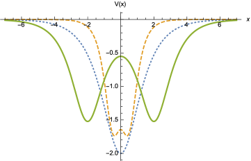
Figure 1: Plot of the potential (21) for 1) $\eta_{1}=.5,\eta_{2}=1.5,\epsilon_{1}=\epsilon_{2}=1$ (dotted curve); 2) $\eta_{1}=1,\eta_{2}=2,\epsilon_{1}=.5,\epsilon_{2}=.6$ (dashed curve); 3) $\eta_{1}=.5,\eta_{2}=.8,\epsilon_{2}=1.5,=\epsilon_{2}=2.6$ (thick curve).

Periodic solutions.— The mKdV equation also admits periodic solutions w3 ; w4 ; KKSH ; Fu . A periodic solution corresponding to one-gap state is given in w3

$$u(x)=V(x)=$$

$$\frac{(a-b)(a+b+c)\,{\rm sn}^{2}(\eta\,x,m)-a(a+2b+c)}{(a-b)\,{\rm sn}^{2}(\eta\,x,m)+(a+2b+c)},$$ (23)

where ${\rm sn}(\eta\,x,m)$ is the Jacobi elliptic function with the modulus $m(0\leq m\leq 1)$

$$m=\left[\frac{(a-b)(a+b+2c)}{(a-c)(a+2b+c)}\right]^{\frac{1}{2}},$$ (24)

and the scale

$$\eta\equiv\frac{1}{2}\left[(a-c)(a+b+c)\right]^{\frac{1}{2}}.$$ (25)

Here $a>b>c$ are constants.

This solution of mKdV equation thus furnishes a periodic potential of the graphene system that admits a zero energy bound state with $k_{y}^{2}=\eta^{2}$.

In the limit $m\to 1(b=c=0)$ , ${\rm sn}\to\tanh$ and $\eta\to a/2$, and $u(x)\to-a\,{\rm sech}\,ax$, which is just the 1-solution case in Eq. (20).

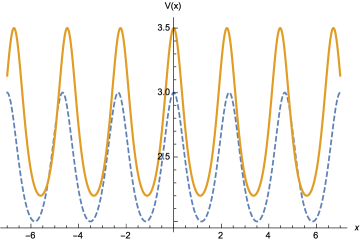
Figure 2: Plot of the potential (mKdV equation approach to zero energy states of graphene) for 1) $a=3,b=2,c=1$ (dashed curve); 2) $a=3.5,b=2.2,c=1.4$ (thick curve).

Other periodic potentials can be obtained from the examples given in KKSH ; Fu . As an example, let us take Fu

$$u(x) = V(x)=-m\,\eta\,{\rm cn}\,\left(\eta\,x,\,m\right);$$ (26)

$$~{}~{}\eta\equiv\sqrt{\frac{a}{2m^{2}-1}}.$$

Here ${\rm cn}\,(x,m)$ is the Jacobi elliptic cosine function with modulus $m$ and $a>0$ is a constant. For $m\to 1,{\rm cn(x,m)}\to{\rm sech~{}x}$ , Eq. (26) reduces to Eq. (20). In Figs 2 and 3 we present visual representations of the potentials (mKdV equation approach to zero energy states of graphene) and (26) for different parameter values.

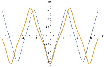
Figure 3: Plot of the potential (26) for 1) $m=.8,a=1$ (dashed curve); 2) $m=.9,a=2$ (thick curve).

Combined KdV and mKdV equation.— The above observation can be extended to other soliton equations. For instance, consider the combined KdV and mKdV equation w3 ; w4

$$u_{t}+6\alpha uu_{x}+6\beta u^{2}u_{x}+u_{xxx}=0,~{}~{}~{}\beta>0.$$ (27)

It turns out that the solution $u(x)$ of this equation is connected to the potential of the Dirac equation by

$$V(x) = \sqrt{\beta}u(x)+\gamma,~{}~{}~{}\gamma\equiv\frac{\alpha}{2\sqrt{\beta}};$$

$$k_{y}^{2} = \eta^{2}+\gamma^{2}.$$ (28)

The $N$-soliton solutions $u(x)$ of Eq.(27) are known w3 . For illustration we present the one-soliton solution

$$u(x)=V(x) = -\frac{2\eta}{\sqrt{\beta}}\,\frac{\sin\theta}{\cos\theta+\cosh 2\eta x},$$

$$\cos\theta = \alpha(\alpha^{2}+4\eta^{2}\beta)^{-1/2}.$$ (29)

Fig 4 shows that the potential (mKdV equation approach to zero energy states of graphene) is a single well one and the depth of the potential can be increased or decreased by choosing the parameters suitably.

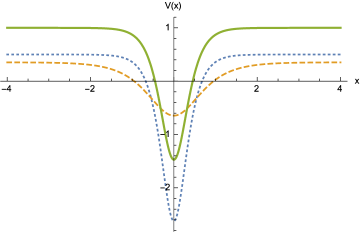
Figure 4: Plot of the potential (mKdV equation approach to zero energy states of graphene) for 1) $\alpha=1,\beta=1,\eta=2$ (dotted curve); 2) $\alpha=1,\beta=2,\eta=1$ (dashed curve); 3) $\alpha=2,\beta=1,\eta=2$ (thick curve).

Summary.— In this Letter we have utilized the relation between the solutions of nonlinear evolution equations, namely, the mKdV equation and combined mKdV and KdV equation and the Dirac equation to find a large number of potentials admitting exactly known zero energy solutions. There are of course many other solutions of the aforementioned equations ZZSZ and depending on the specific need of the problem or experiment some of these solution can play an important role.

————–