Pareto Smoothed Importance Sampling

Abstract

Importance weighting is a general way to adjust Monte Carlo integration to account for draws from the wrong distribution, but the resulting estimate can be highly variable when the importance ratios have a heavy right tail. This routinely occurs when there are aspects of the target distribution that are not well captured by the approximating distribution, in which case more stable estimates can be obtained by modifying extreme importance ratios. We present a new method for stabilizing importance weights using a generalized Pareto distribution fit to the upper tail of the distribution of the simulated importance ratios. The method, which empirically performs better than existing methods for stabilizing importance sampling estimates, includes stabilized effective sample size estimates, Monte Carlo error estimates, and convergence diagnostics. The presented Pareto $\hat{k}$ finite sample convergence rate diagnostic is useful for any Monte Carlo estimator.

Keywords: importance sampling, Monte Carlo, Bayesian computation

1 Introduction

Importance sampling is a simple modification to the Monte Carlo method for computing expectations that is useful when there is an auxiliary distribution $g(\theta)$ that is easier to directly sample from than the target distribution $p(\theta)$, which may be only known up to a proportionality constant (Hammersley and Handscomb,, 1964). The starting point is the simple Monte Carlo estimate for the expectation of a function $h$,

$$I_{h}=\operatorname{\mathrm{E}}_{p}(h)=\int h(\theta)p(\theta)\,d\theta\approx\frac{1}{S}\sum_{s=1}^{S}h(\theta_{s}),$$

which requires exact draws $\theta_{s},\ s=1,\dots,S$ from $p(\theta)$. The self-normalized importance sampling estimate for the same expectation is

$$\frac{\sum_{s=1}^{S}r_{s}h(\theta_{s})}{\sum_{s=1}^{S}r_{s}},\qquad r_{s}=r(\theta_{s})=\frac{p(\theta_{s})}{g(\theta_{s})},$$ (1)

which only requires draws $\theta_{s}$ from a proposal distribution $g(\theta)$.

The success of the importance sampling estimator depends on the distribution of the importance ratios $r_{s}$ and of $r_{s}h(\theta_{s})$. When the proposal distribution is a poor approximation to the target distribution, the distribution of importance ratios can have a heavy right tail. This can lead to unstable importance weighted estimates, sometimes with infinite variance.

Textbook examples of poorly performing importance samplers occur in low dimensions when the proposal distribution has lighter tails than the target, but it would be a mistake to assume that heavy-tailed proposals will always stabilize importance samplers. This intuition is particularly misplaced in high dimensions, where importance sampling can fail even when the ratios have finite variance. MacKay, (2003, Section 29.2) provides an example of what goes wrong in high dimensions: the ratios $r_{s}$ can vary by several orders of magnitude and the estimator (1) will be dominated by a few draws. Hence, even if the approximating distribution is chosen so that the importance ratios are bounded so that (1) has finite variance, the bound can be so high and the variance so large that the behavior of the self-normalized importance sampling estimator is practically indistinguishable from an estimator with infinite variance. This suggests that if we want an importance sampling method that works in high dimensions, we need to move beyond being satisfied with estimates that have finite variance and find methods with built-in error assessment.

In this paper, we

• propose Pareto smoothed importance sampling (PSIS), a method for stabilizing importance sampling estimates;

• show that PSIS has the usual properties for a well-behaved self-normalized importance sampling estimator such as consistency and finite variance;

• propose a simple numerical Pareto $\hat{k}$ diagnostic for finite sample convergence rate suitable for any Monte Carlo estimator;

• demonstrate the behavior of PSIS and $\hat{k}$ in several low and high-dimensional examples.

This paper focuses on self-normalized importance sampling, but Pareto $\hat{k}$ diagnostic and Pareto smoothing can be used also for ordinary importance sampling or any Monte Carlo estimate, as demonstrated in some of the references discussed in Section 6. Beyond the examples in the latter part of this paper, PSIS forms the basis for the widely-used loo R package for stable, high-dimensional leave-one-out cross-validation (Vehtari et al.,, 2017, 2018). This package has been downloaded more than two million times. PSIS has been also implemented, for example, in the widely used Python packages ArviZ (Kumar et al.,, 2019) and Pyro (Bingham et al.,, 2019).

2 Stabilizing importance sampling estimates by modifying the ratios

The stability of self-normalized importance sampling methods can be improved by directly modifying the computed ratios. For notational convenience, we rewrite these importance samplers as,

$$\int h(\theta)p(\theta)\,d\theta\approx\frac{\sum_{s=1}^{S}w_{s}h(\theta_{s})}{\sum_{s=1}^{S}w_{s}},$$ (2)

where $w_{s}=r_{s}$ would recover the standard self-normalized importance sampler.

Ionides, (2008) showed that the truncation rule,

$$w_{s}=\min{\left(r_{s},\sqrt{S}\bar{r}\right)},$$ (3)

where $\bar{r}$ is the average of the original $S$ importance ratios, is simulation-consistent with finite variance. The critical advantage conveyed by the truncation is that these properties now extend to problems that only have integrable ratios: we get finite variance under the assumption that $\mathbb{E}(|r_{s}|)<\infty$ instead of under the stronger condition $\mathbb{E}(|r_{s}|^{2})<\infty$ which is needed for the unmodified importance sampling estimator (1) to have finite variance.

This simple modification to the raw importance ratio greatly extends the range of problems for which the estimator has finite variance. Unfortunately, while the truncation can improve the stability of the weights, our experiments show that the simple weight modification scheme can be too severe, leading to larger than necessary finite sample bias.

2.1 Modeling the tail of the importance ratios

In this paper, we propose a new scheme for modifying the extreme importance ratios that adapts more readily to the problem under consideration than the universal truncation rule of Ionides, (2008).

To motivate the new scheme, we begin by noting that the success of plain importance sampling depends on how many moments $r(\theta)$ and $h(\theta)r(\theta)$ possess, with the estimator having finite variance if at least two moments exist. This suggests that using information about the distribution of $r_{s}|r_{s}\!>\!u$, for some threshold $u\rightarrow\infty$ as $S\rightarrow\infty$, should allow us to improve the quality of our importance sampling estimators.

Pickands, (1975) and Balkema and de Haan, (1974) proved, under commonly satisfied conditions, that as the sample size increases, the distribution of $r_{s}|r_{s}\!>\!u$ is well approximated by the three-parameter generalized Pareto distribution,

$$p(y\mid u,\sigma,k)=\begin{cases}\frac{1}{\sigma}\left(1+k\left(\frac{y-u}{\sigma}\right)\right)^{-\frac{1}{k}-1},&k\neq 0\\ \frac{1}{\sigma}\exp\left(\frac{y-u}{\sigma}\right),&k=0,\end{cases}$$ (4)

where $u$ is a lower bound parameter, $y$ is restricted to the range $(u,\infty)$, $\sigma$ is a non-negative scale parameter, and $k$ is an unconstrained shape parameter. The generalized Pareto distribution has $1/k$ finite fractional moments when $k>0$, and thus we can infer the number of existing fractional moments of the weight distribution by focusing on $k$.

To estimate the parameters in the generalized Pareto distribution, we use the $M$ largest importance ratios, where

$$M=\min(0.2S,3\sqrt{S}).$$

Restricting the tail modeling to a subset of the largest importance ratios implicitly defines a value of $u$ in the Pareto distribution. The above rule for $M$ was made based on extensive computational theory, related suggestions in the literature (Scarrot and MacDonald,, 2012), and in line with the requirements for consistent estimation (Pickands,, 1975). The minimum tail proportion $0.2$ reduces the possible bias for small $S$, with the square root rule providing stability when $S$ is high. In practice, we have found the method to be insensitive to the exact form of $M$; for instance, using $M=0.2S$ in all cases was suggested by Vehtari et al., (2017), and it worked well even though it is not asymptotically correct. We tested several other methods reviewed by Scarrot and MacDonald, (2012) for selecting $u$ directly, but found them to have higher variability than this simple heuristic, leading to increased variance in estimating $k$.

The scale and shape parameters, $\sigma$ and $k$, can be estimated using the highly efficient, low-bias approximate Bayesian method of Zhang and Stephens, (2009), which we briefly review in Appendix F. We choose this approach due to its efficiency and its ability to be used automatically without human intervention. In Appendix G we describe additional practical regularization of the estimate $\hat{k}$, which helps to reduce the variance of the estimate when $S$ is small, without affecting its asymptotic properties.

Although in most cases we cannot verify that the distribution of $r_{s}$ lies in the domain of attraction for an extremal distribution, we will use this as a working assumption for building our method. Pickands, (1975) notes that “most ‘textbook’ continuous distribution functions” lie in the domain of attraction of some extremal distribution function. For finite $S$, we could alternatively interpret $\hat{k}$ as saying that the sample $(r(\theta_{s}))_{s=1}^{S}$ is not statistically distinguishable from a sample of size $S$ from a distribution with tail index $\hat{k}$.

Input: Raw importance ratios $r_{s}$, $s=1,\ldots,S$, ordered from lowest to highest

Output: PSIS-smoothed importance weights $w_{s}$, $s=1,\ldots,S$

Set $M=\min(0.2S,3\sqrt{S})$;

Set $w_{s}=r_{s}$, $s=1,\ldots,S-M$;

Set $\hat{u}=r_{S-M}$;

Estimate $(\hat{k},\hat{\sigma})$ in the generalized Pareto distribution with cutpoint $\hat{u}$ from the $M$ largest importance ratios, using the algorithm of Zhang and Stephens, (2009) with the additional prior described in Appendix G;

Set $w_{S-M+z}=\min\left(F^{-1}\left(\frac{z-1/2}{M}\right),\max_{s}(r_{s})\right)$, for each $z=1,\ldots,M$;

If the estimated shape parameter $\hat{k}$ exceeds 0.7, report a warning that the resulting importance sampling estimates are likely to be unstable.

Algorithm 1 PSIS procedure for computing importance weights.

2.2 Our proposal: Pareto smoothed importance sampling

We propose a new method to stabilize the importance weights by replacing the $M$ largest weights above the threshold $u$ by a set of well-spaced values that are consistent with the tails of the importance distribution,

$$w_{S-M+z} =F^{-1}\left(\frac{z-1/2}{M}\right)$$

$$=u+\frac{\sigma}{k}\left(\left(1-\frac{z-1/2}{M}\right)^{-k}-1\right),$$

where $z=1,\dots,M$, and $F^{-1}$ is the inverse-CDF of the generalized Pareto distribution fitted to the $M$ largest importance ratios. The inverse transformation corresponds to a fast approximation of the expected ordered statistics (Blom,, 1958), with increasing accuracy as $M$ increases. Expected ordered statistics provide low bias and reduced variance compared to the original ratios or ordered random draws from the distribution.

We show that replacing the largest ratios with the expected ordered statistics changes PSIS to have finite variance and error distribution converging to normal, when $k\in(0.5,1)$. Section 3 shows how to model the PSIS error distribution as mean of truncated Pareto variables with truncation corresponding to the largest expected ordered statistics. Section 4 provides finer details proving that the PSIS estimator, summarized in Algorithm 1, is simulation-consistent and has finite variance under relatively light conditions. The final step in the algorithm warns the user if the estimated shape parameter $\hat{k}$ in the generalized Pareto distribution is larger than $0.7$. This is an automatic stability check that we justify in Section 3.

When Pareto $\hat{k}$ is less than 0.7, we recommend estimating the Monte Carlo standard error (MCSE) of PSIS using the estimator of Owen, (2013, Ch. 9) (see also Elvira et al.,, 2022) for self-normalized importance sampling,

$$\widehat{\widetilde{\operatorname{\mathrm{Var}}}}(\hat{I}_{h}^{S}) \approx \sum_{s=1}^{S}\tilde{w}_{s}^{2}(h(\theta_{s})-\tilde{\mu})^{2},\mbox{ \ \ for independent draws}$$ (6)

$$\sum_{s=1}^{S}w_{s}^{2}(h(\theta_{s})-\tilde{\mu})^{2}/R_{\mathrm{eff,MCMC}},\mbox{ \ \ for MCMC draws},$$

where $\tilde{w}_{s}=w_{s}/\sum_{s^{\prime}=1}^{S}w_{s^{\prime}}$ are normalized weights, $\tilde{\mu}=\sum_{s=1}^{S}\tilde{w}_{s}h(\theta_{s})$, and $R_{\mathrm{eff,MCMC}}=S_{\mathrm{eff,MCMC}}/S$ is the relative efficiency of MCMC, and the effective sample size $S_{\mathrm{eff,MCMC}}$ for $h(\theta)$ is computed using the split-chain method (Vehtari et al.,, 2021).

The corresponding effective sample size estimate is

$$\mathrm{ESS}_{h}\approx\frac{\sum_{s=1}^{S}(h(\theta_{s})-\tilde{\mu})^{2}}{\widehat{\widetilde{\operatorname{\mathrm{Var}}}}(\hat{I}_{h}^{S})}.$$ (7)

When $h(\theta)=1$, this simplifies to

$$\mathrm{ESS}\approx 1/{\sum_{s=1}^{S}\tilde{w}_{s}^{2}},$$ (8)

which is the effective sample size estimate for the zeroth moment (normalizing term). Expression (8) is also the generic effective sample size estimate proposed by Kong, (1992) (see also Kong et al.,, 1994; Owen,, 2013; Elvira et al.,, 2022), which doesn’t depend on $h$.

Chatterjee and Diaconis, (2018) warn against using a variance estimator as an importance sampling diagnostic, as it depends on the accuracy of an estimate obtained by importance sampling itself, and they recommend using a “diagnostic that is not itself an importance sampling estimate of any quantity.” Pareto $\hat{k}$ is such a diagnostic, and we validate these approximations using the examples in Sections 3 and 5, and Appendix D, demonstrating good behavior when the estimated shape parameter in the generalized Pareto distribution is less than $0.7$.

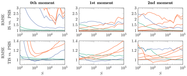
Figure 1: For Example 1, the ratio of root mean squared error (RMSE, computed from 1000 simulations) between importance sampling (IS), truncated importance sampling (TIS), and Pareto smoothed importance sampling (PSIS) for zeroth, first $(h(\theta)=\theta)$, and second $(h(\theta)=\theta^{2})$ moments. A ratio greater than $1$ means PSIS had lower RMSE than its competitor. The target distribution is $\operatorname{\mathrm{exponential}}(1)$ and the proposal distribution is exponential with rate (inverse mean) parameter $\theta\in(1.3,1.5,2,3,4,10)$. The lines are colored according to the $\hat{k}$ (for zeroth moment) and $\hat{k}_{h}$ (for first and second moment) estimates. Green lines have $\hat{k}<0.5$, blue lines have $\hat{k}\in(0.5,0.7)$, and red lines have $\hat{k}>0.7$.

The following example shows how PSIS compares with simple importance sampling (IS) and truncated importance sampling (TIS) for a simple one-dimensional example (with repeated simulations). Further simulated examples in low and moderate dimensions can be found in Section 3 and Appendix D.

Example 1.

Consider the following one-dimensional example where the target distribution is $\operatorname{\mathrm{exponential}}(1)$ and the proposal distributions are $\operatorname{\mathrm{exponential}}(\theta)$ for $\theta\in(1.3,1.5,2,3,4,10)$, with the exponential distribution parameterized by the rate (inverse mean) parameter $\theta$. The importance ratios will have infinite variance whenever $\theta>2$ (Robert and Casella,, 2004).

Figure 1 shows the ratio of root mean square errors (RMSEs) computed from 1000 simulations, comparing ordinary (IS), truncated (TIS), and Pareto smoothed importance sampling (PSIS). In all cases a ratio larger than $1$ corresponds to PSIS having the lower RMSE. It is clear that PSIS is always better than straight IS. On the other hand, PSIS is slightly worse than TIS with intermediate sample sizes for $\theta=2$, which corresponds to $\hat{k}\approx 0.5$. A likely reason for this is that in this case the truncation rule in TIS is perfectly calibrated for the weight distribution and hence it is the best possible scenario for TIS. Deviations from this scenario lead to PSIS performing better. This is the only example we found where TIS outperformed PSIS. Figure 13 in Appendix D shows the distribution of the weights and estimates over several runs for this example when $\theta=3$. From this, we see that PSIS yielded smaller bias but slightly larger variance than TIS. We further explore this example in Appendix D.1.

3 Using $\hat{k}$ as a diagnostic

As part of the PSIS procedure, we estimate the shape parameter $k$ of the limiting generalized Pareto distribution for the upper tail of the importance ratios. A simple option would be to use this estimate $\hat{k}$ and trust importance sampling as reliable if $\hat{k}<0.5$, as it would indicate that the variance is finite and the central limit theorem holds. Our theory shows, however, that PSIS leads to valid and well-behaved importance sampling routines for any integrable density. This suggests that requiring the estimated shape parameter be less than $0.5$ will be unnecessarily stringent.

Occasionally, we will use a $h$-specific tail estimate $\hat{k}_{h}$ for the tails of the distribution $h(\theta)r(\theta)$, $\theta\sim g(\theta)$. This can be useful when $h(\theta)$ is unbounded, or goes to zero, as it is possible if $h$ grows fast enough (or goes to zero fast enough) relative to $r(\theta)$ that the tail behavior of $r(\theta)h(\theta)$ can be qualitatively different from the tail behavior of $r(\theta)$. As $h(\theta)$ can be negative for some $\theta$ (e.g., when $h(\theta)=\theta$), we estimate $\hat{k}$ for both left and right tails of $h(\theta)r(\theta)$ and set $\hat{k}_{h}$ to that $\hat{k}$ which is bigger. Although in this paper we focus on using $\hat{k}$ as a diagnostic for PSIS, $h$-specific tail estimate $\hat{k}_{h}$ is useful also when using regular or quasi Monte Carlo (i.e., $r(\theta)=1$). We validate the $h$-specific $\hat{k}_{h}$ in Appendix D.

3.1 PSIS is reliable when $k<0.7$

Extensive experiments show that for typical moderate sample sizes used in practice, PSIS gives reliable (that is, low-bias, low variance) estimators of $I_{h}$ when $\hat{k}_{h}<0.7$. This can be interpreted as the estimate being reliable when the sample used to compute the PSIS estimate is indistinguishable from one that comes from a density with more than $0.7^{-1}\approx 1.4$ finite fractional moments. When $\hat{k}_{h}>0.7$ (less than $1.4$ finite fractional moments) the convergence of the estimator becomes too slow to be useful in many practical cases. We provide theoretical support of this threshold. We also provide a sample-size-specific threshold, that can be useful when having very small or very big sample size.

In this section, we make the distinction between the true but unknown $k$ and our finite sample estimate $\hat{k}$ as a way to understand the differences between the asymptotic behavior of PSIS and its finite sample behavior. We first show theoretically that the computational complexity of importance sampling has a meaningful qualitative change around $k=0.7$. The finite sample estimate $\hat{k}$ is a useful indicator of the practical pre-asymptotic convergence rate of PSIS even when the distribution of ratios is bounded and has finite variance. In particular, we show that $\hat{k}$ can identify poorly behaved but finite variance proposals in high dimensions.

3.2 Pareto means and central limit theorems

Section 4 proves asymptotic consistency and finite variance. In this section we use various large sample results to characterize finite sample behavior of IS, TIS, and PSIS. There is no strict rule what large sample means in each case, but the theory based results are able to explain many empirical results shown by our experiments.

We analyse the properties of IS, TIS, and PSIS using the generalized central limit theorem and distribution of sum of non-truncated and truncated Pareto distributed variables. In addition we use distribution of sum of truncated Pareto distributed variables separately to explain why $\hat{k}>0$ is a useful pre-asymptotic finite sample diagnostic when the bound of the bounded ratios is large.

3.2.1 Generalized central limit theorem

The distribution of the mean of i.i.d. variables from a distribution with Pareto (power law) tails can be approximated with a stable distribution (e.g. Uchaikin and Zolotarev,, 1999, p. 62). If the tail index $k<0.5$, the central limit theorem holds and the stable distribution is normal, scaling as $S^{-1/2}$ (as $S\rightarrow\infty$). For $k=0.5$ that stable distribution is a normal distribution that scales as $(S/\log(S))^{-1/2}$, and for $k\in(0.5,1)$ the stable distribution has stability parameter $1/k$ and scales as $S^{(k-1)}$ (as $S\rightarrow\infty$). The CLT and GCLT results for $k\neq 1/2$ are usually mentioned for $S\rightarrow\infty$, while the result for $k=0.5$ is reported conditional on $S$. We also sometimes refer to these well known results as is, but for finite $S$ the transition from $k<0.5$ via $k=0.5$ to $k>0.5$ is smooth. We eventually provide also an approximate smooth scaling rate for PSIS conditional on finite $S$.

We first consider just the estimation of the normalization term, that is the expectation of the ratios, which is already useful as this is what is needed, for example, in fast leave-one-out cross-validation (Vehtari et al.,, 2017). To further simplify, we first consider just the tail part, which we assume is well approximated by Pareto distribution.

3.2.2 Pareto means and IS L1 deviation

For $k\in(0.5,1)$, the explicit expressions for the densities of stable distributions are unknown, and numerical algorithms are needed. Zaliapin et al., (2005, Eq. (28)) provide a closed form approximation of quantile $q>0.95$ for the sum of Pareto-distributed variables. To get the corresponding approximation for the mean, we simply divide by $S$ to get

$$S^{(k-1)}(1-q)^{-k}+\mu,$$ (9)

where $\mu$ is the expected mean. As the distribution of ratios are right skewed, the distribution of mean will be also right skewed, and thus the absolute L1 deviation for the mean will be less than $S^{(k-1)}(1-q)^{-k}$ with probability $q$.

Thus to control the L1 deviation when $k$ increases beyond 0.5, $S$ needs to grow proportionally to

$$(c_{1}(1-q)^{-k})^{1/(1-k)},$$ (10)

where $c_{1}$ includes also the effect of the scale of the distribution in more general case. Zaliapin et al., (2005) provide more accurate numerical approximations of quantiles of the Pareto sum distribution (that can be used also for quantiles of mean distribution), but the accuracy of (9) and (10) is sufficient for our purposes when examining the L1 deviation of IS with raw ratios.

3.2.3 Truncated Pareto means and PSIS RMSE

PSIS replaces the largest ratios with their expected ordered statistics. The mean of the expected ordered statistics is not the same as the expectation of mean of raw ratios. With thin-tailed distributions the difference is usually small, but for thick-tailed distributions we need to take the difference into account. The effect of replacing the largest ratios with the expected ordered statistics is similar to truncating with the largest expected ordered statistic.

Truncation makes PSIS have finite variance (see Sections 2.2 and 4) with the price of introducing bias. We can derive analytically the mean and variance of the truncated Pareto mean; see Appendix A and Zaliapin et al., (2005), Eqs. (60) and (61). The generalized central limit theorem states that the largest expected ordered statistic scales as $S^{k}$; see, e.g., Bouchaud and Georges, (1990), p. 138. By substituting $S^{k}$ in the truncated mean and variance equations (see Appendix A), we see that standard deviation of PSIS scales approximately as $S^{-1/2}$ when $k<0.5-0.5/\log_{10}(S)$, as $(S\log(S))^{-1/2}$ when $k=0.5$, and as $S^{k-1}$ when $k\in(0.5+0.5/\log_{10}(S),1)$. The bias of PSIS is negligible when $k\leq 0.5$, and the bias scales approximately as $S^{k-1}$ when $k\in(0.5+0.5/\log_{10}(S),1)$. The scaling between the above-mentioned ranges and $k=1/2$ changes smoothly. When $k\in(0.5+0.5/\log_{10}(S),1)$, to control PSIS RMSE, $S$ needs to scale proportionally to

$$c_{2}^{1/(1-k)}.$$ (11)

Based on the numerical experiments, $1/c_{2}$ matches the target RMSE. Using a rule of 10%, we get a rule of thumb, $S=10^{1/(1-k)}$. We can derive from the estimated minimum required sample size also an approximate ESS given $k$ as

$$\mathrm{ESS}_{k}\approx S/10^{k/(1-k)}.$$ (12)

This is an optimistic estimate as it doesn’t take into account the variance of the weights, but it is useful to set expectations on sample size given observed $\hat{k}$. Although Eqs. (11) and (12) are derived for $k\in(0.5+0.5/\log_{10}(S),1)$, they turn out to be surprisingly good approximations also for $k\leq 0.5+0.5/\log_{10}(S))$, as the scale of the error distribution depends on $k$.

Eqs. (11) and (12) are meant only to give guidance on the order of magnitude for the required sample size. When the sample size is sufficient and $\hat{k}<0.7$, a more accurate estimate of RMSE can be obtained using the variance (Eq. (6)), and then given the convergence rate estimate discussed in Section 3.2.6, a more accurate estimate of the required sample size to reach the required RMSE can be obtained. Especially when $\hat{k}<0.5-0.5/\log_{10}(S)$ (see Section 3.2.6), we may assume the variance based RMSE and ESS estimates to be much more accurate than the above approximations depending only on $k$.

Based on numerical analysis of truncated Pareto means, when $k<0.7$ the variance dominates the PSIS RMSE. This explains why the variance based MCSE estimate (Eq. (6)) works well for PSIS also when $k>0.5$ (as demonstrated by the examples). Due to the Pareto smoothing of $M$ largest weights, the PSIS RMSE is smaller than if only plain truncation at high upper quantile was used. When $k>0.7$, independently of $S$ the effect of bias dominates and the variance based MCSE starts to fail (also demonstrated by the examples). Although the accuracy can be improved by increasing $S$, diagnosing the accuracy is more difficult. This provides additional justification for the $0.7$ threshold. When the variance dominates the RMSE, we can also directly use the generalized CLT truncated variance result to justify the scaling of RMSE; see, e.g., Bouchaud and Georges, (1990), p. 138.

TIS truncates at $\bar{r}S^{1/2}$, which reduces variance but increases bias. Due to a high bias of TIS, the variance based MCSE estimate for TIS starts to fail when $k>0.5$; see results in Appendix D.1. Eventually for larger $k$, the dominating bias makes the TIS RMSE scale as $S^{0.5-0.5/k}$ (see Appendix A); that is, TIS RMSE increases much faster than PSIS RMSE when $k>0.5$.

RMSE is not well defined for IS, as the variance of the raw ratios is infinite when $k>0.5$, although we get finite estimate when running finite number of simulations; see Appendix A.

Figure 2 shows the theoretical approximation and empirical result for PSIS RMSE, when the ratios are exactly Pareto distributed. The simulations match the simple theoretical approximation well even for $k\leq 0.5$, although a different approximation would be more appropriate for $k<0.5+0.5/\log_{10}(S)$.

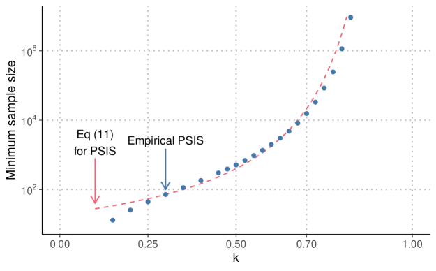
Figure 2: Minimum sample size (red dashed line) required to control RMSE of PSIS as a function of $k$, as computed according to the heuristic (11), and empirical PSIS result (blue dots) for the average sample size to obtain fixed RMSE (from 10 000 repeated simulations). The required sample size quickly grows infeasibly large when $k>0.7$.

Appendix D.1 presents more details on the simulation and more results.

3.2.4 Sample size dependent $\hat{k}$-threshold

Based on the bias-variance tradeoff threshold and extensive experiments for moderate sample sizes, threshold $\hat{k}<0.7$ is a good choice. We can also reverse the minimum sample size requirement to make a sample-size-specific threshold. Based on the experiments, the appropriate constant is such that an easy to remember thumb rule (for $S\geq 10$) is

$$1-1/\log_{10}(S).$$ (13)

Sample sizes 1000, 2000, 4000, and 10 000 correspond to thresholds $0.67$, $0.7$, $0.72$, and $0.75$, which can all be approximated with a generic threshold $0.7$. For a much smaller sample size 100, the threshold would be $0.5$, and for a much bigger sample size $100\,000$ the threshold would be $0.8$. Although with bigger sample size $S$ we can achieve estimates with small probability of large error, it is difficult to get accurate MCSE estimates as the bias starts to dominate when $k>0.7$ (see Section 3.2.3).

3.2.5 PSIS vs IS L1 deviation

The normal approximation of the distribution of truncated mean can also be used to approximate quantiles and L1 deviation. Zaliapin et al., (2005) propose to use this for lower quantiles for which it can be expected to be more accurate, but based on our experiments the approximation is useful to give approximate order of the magnitude for upper quantiles, too. For the raw ratios the quantile was given above as $S^{k-1}(1-q)^{-k}$, but for PSIS we can use approximation

$$S^{k-1}\Phi^{-1}(q).$$ (14)

As normal distribution has shorter tail than a stable distribution with tail index $k>0.5$, we can see that PSIS has smaller L1 deviation than IS, when $k>0.5$. Figure 3 shows the empirical and theoretical results for L1 deviation with IS and PSIS ($q=0.99$).

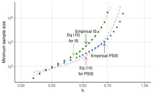
Figure 3: Minimum sample size (red dashed line) required to control L1 deviation by PSIS as a function of $k$, as computed according to the heuristic (14), empirical PSIS result (blue dots) for the average sample size to obtain fixed L1 deviation, minimum sample size (yellow line) required to control L1 deviation by IS as a function of $k$, as computed according to the heuristic (10), empirical IS result (green dots) for the average sample size to obtain fixed L1 deviation (from 10 000 repeated simulations). The required sample size grows more quickly for IS than PSIS, and for PSIS quickly grows infeasibly large when $k>0.7$.

3.2.6 PSIS RMSE convergence rate given $\hat{k}$

In addition to considering how $S$ needs to change to control the error when $k$ increases, it is useful to consider how $S$ needs to change to decrease the error given fixed $k$. PSIS RMSE scaling given different values of $k$ were given in Section 3.2.3.

If we consider CLT convergence rate to have efficiency 1, and write $(S^{-1/2})^{\alpha},\alpha=1$, we can calculate the relative efficiency $\alpha$, when $k\in(0.5+0.5/\log_{10}(S),1)$ and $k=0.5$. By solving $\alpha$ from $S^{k-1}=(S^{-1/2})^{\alpha}$ and $(S/\log(S))^{-1/2}=(S^{-1/2})^{\alpha}$, we find that the relative efficiencies for $k\in(0.5+0.5/\log_{10}(S),1)$ and $k=0.5$ are $2(1-k)$ and $1-1/\log(S)$, respectively (see Appendix B). The relative convergence rate changes smoothly, but piecewise linear approximation with knots at $0$, $0.5-0.5/\log_{10}(S)$, $0.5$, $0.5+0.5/\log_{10}(S)$, and $1$, is useful for characterizing how the relative convergence rate changes with $k$ (see Appendix B).

Figure 4 shows theoretical and experimental convergence rate for PSIS RMSE in case of ratio distribution being exactly Pareto distribution. Empirical convergence rate is estimated by dividing the PSIS RMSE of a bigger sample size with the PSIS RMSE of a smaller sample size. The sample sizes in Figure 4 are $3000$ and $10\,000$. Empirical results show that the convergence efficiency starts to drop before $k=0.5$ and matches theoretically predicted efficiency at $k=0.5$. The figure also shows a smooth approximation of the theoretical convergence rate; see the equation and piecewise linear approximation in Appendix B.

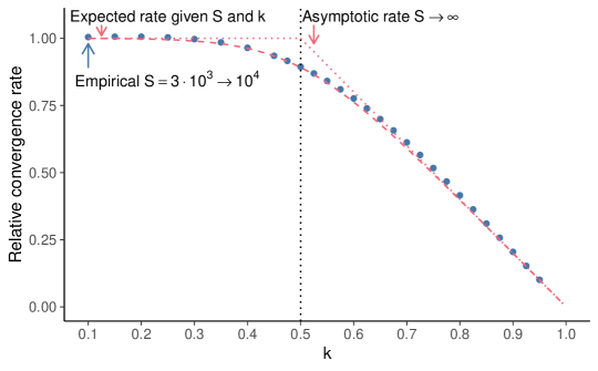
Figure 4: Convergence rate as a function of $k$ and $S$. Red dashed line shows the theoretical convergence rate based on the CLT and generalized CLT. Blue dots show the empirical convergence rate from the simulation with Pareto distributed ratios (from 10 000 repeated simulations). Empirical convergence rate is estimated by how much the error decreases when the sample size is doubled $(5\,000\rightarrow 10\,000)$. For a finite sample size $S$ the transition from CLT convergence rate to GCLT convergence rate is smooth, and the there is no sudden change at $k=0.5$.

Given a sample size $S$, the relative convergence rate results can be used to predict how much bigger sample size is needed to halve the PSIS RMSE. For example if $k=0.7$ approximately $4^{(1/0.7)}\approx 10$ times bigger sample size is needed to halve PSIS RMSE. This empirical result matches the theory well, as the ratio distribution is exactly Pareto distributed. When the ratio distribution is not exactly Pareto distributed, the shape of the bulk and unobserved part of the tail influence the convergence rate, and the above theoretical results should be considered only as approximate guidance. Section 3.3 and Appendix D contain examples of convergence rates when the bulk of the ratio distribution does not follow Pareto distribution.

Appendix B.1 includes more results, and Table 1 summarizes the useful diagnostic equations discussed above.

Minimum sample size for reliable Pareto smoothed estimate	$10^{(1/(1-\hat{k}))}$	(3.2.3)
Approximate ESS given $\hat{k}$	$S/10^{(\hat{k}/(1-\hat{k}))}$	(3.2.3)
Maximum $\hat{k}$ for reliable Pareto smoothed estimate	$1-1/\log_{10}(S)$	(3.2.3)
Maximum $\hat{k}$ for low bias in Pareto smoothed estimate	0.7	(3.2.3)
Convergence rate when $k<0.5-0.5/\log_{10}(S)$	$\sim S^{1/2}$	(3.2.6)
Convergence rate when $k=0.5$	$S^{(1-1/\log(S))/2}$	(3.2.6)
Convergence rate when $k>0.5+0.5/\log_{10}(S)$	$\sim S^{(1-k)}$	(3.2.6)

Table 1: Summary of useful diagnostics related to PSIS RMSE and the convergence rate. The number $10$ used in the four first equations is an ad hoc choice based on rule of $10\%$ and empirical results.

3.2.7 Only the tail has Pareto shape

In practice, the distribution of the ratios is not exactly Pareto distributed. If the tail index $k<0.5-0.5/\log_{10}(S)$ (as discussed in Section 3.2.3), the variance-based MCSE based on all ratios is accurate, and the exact shape of the ratio distribution has a smaller effect. If the tail index $k$ is close to $0.5$ or larger, the tail behavior dominates the distribution of the mean and the needed sample size can be estimated from $\hat{k}$. The generalized central limit theorem states that mean of any distributions that have Pareto-like tails, converge toward stable distribution with the same tail shape. The result by Pickands, (1975) states that many distributions have tails that can be approximated with the generalized Pareto distribution, which has an additional scale parameter that contributes to the constant $c$ in the needed sample size to obtain a specified error threshold.

3.2.8 $h$-specific estimates

We smooth only $r(\theta)$, and Section 4 discusses assumptions needed for $h$, so that PSIS has asymptotic consistency and finite variance. Under these conditions, the above results extend to the analysis of $h(\theta)r(\theta)$, although now there can be a thick tail both left and right, and the tails may have different tail index. The tail with the larger tail index dominates, and thus we set $\hat{k}_{h}$ to that $\hat{k}$ which is bigger, as discussed in Section 3. In self-normalized importance sampling, there is a ratio of sums. The denominator is always strictly positive and can be viewed as importance weighting with $h=1$, whose $h$-specific $\hat{k}_{h}$ is the original $\hat{k}$. Stability of the ratio will be dominated by the term which has higher $k$ index. For example, in case of $h(\theta)=\theta$ or $h(\theta)=\theta^{2}$, the numerator has higher $k$ index. In fast leave-one-out cross-validation, $h=1/r$ and the denominator has higher $k$ index. The empirical results in this paper support that larger of $\hat{k}_{h}$ or $\hat{k}$ for the normalization term indicates the overall performance. The empirical results support that despite the deviations from the theory for perfect (truncated) Pareto sums, the diagnostics are sufficiently accurate to be useful.

3.2.9 Finite sample size and bounded ratio distributions

With finite sample size, the proposal distribution affects how far from the tail of the ratio distribution we are likely to get draws. Previously we used distribution of mean of truncated Pareto variables to explain the behavior of PSIS replacing the largest weights with the expected order statistics. We can use the truncated Pareto to explain also behavior when the raw ratios are bounded, but the bound is much further in tail than the largest observed ratio. For a bounded distribution, true $k<0$, all moments are finite, and CLT holds asymptotically. If the bound is far from the observed values, pre-asymptotically the mean behaves statistically as if the distribution has not been truncated (see, e.g. Zaliapin et al.,, 2005), $\hat{k}$ can be larger than $0$, and high sample size may be needed before the effect of the truncation is observed. A practical consequence is that even if the proposal distribution had been chosen to guarantee bounded ratios, it is possible that we do not observe raw ratios near the bound. We can approximate tails of bounded ratio distributions with a truncated Pareto distribution, and if the bound is larger than any of the observed ratios, we can proceed using $\hat{k}$ diagnostics as discussed above. Furthermore, the ratios of proper densities have finite mean by construction, and thus $k<1$ always, but pre-asymptotically we can observe $\hat{k}>1$, and the sum then behaves statistically as if the distribution has no finite mean. We demonstrate in the next section that in high dimensions, it is likely that the bound is far and the pre-asymptotic diagnostics work well. We illustrate the behavior in case of bounded ratios in Section 3.3 with an example where eventually $\hat{k}>1$, and in Appendix D.2 with an example where the bound is not initially observed, but with increasing sample size is eventually observed.

It would be possible to construct also an artificial example where the tail would look thin (low Pareto $\hat{k}$) for small $S$ with large probability, while the true tail is thick (high Pareto $\hat{k}$). Chatterjee and Diaconis, (2018) present one such example with a discrete distribution. Except for very small $S$, in all the simulations and applications where we have applied Pareto $\hat{k}$ diagnostic, we have not observed such behavior.

3.3 $\hat{k}$ is a good convergence diagnostic in finite samples and in high dimensions

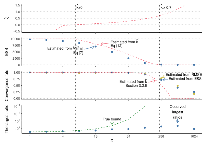
Figure 5: First plot: $\hat{k}$ diagnostic. Asymptotically $k<0$, but with a finite sample size the behavior is statistically as predicted by $\hat{k}$. The vertical dotted lines mark when the tail looks like unbounded $(\hat{k}>0)$, and when the sample size is too small $(\hat{k}>0.7)$. Second plot: estimated effective sample size using Eq. (8) and estimated effective sample size by $S/10^{(1/(1-k))}$. By $D=128$, the $S=10\,000$ importance weighted draws have only a few practically non-zero weights. Third plot: convergence rate estimated by comparing RMSE using $S=5\,000$ and $S=20\,000$ (half and double of original $S$). Convergence rate estimated from $\hat{k}$. By $D=512$ the convergence rate is about $S^{1/4}$, and getting any improvement in the accuracy becomes tedious. The observed convergence rate is higher than predicted by $\hat{k}$ as the weight distribution is not exactly Pareto shaped and the reduction in bias with increasing sample size dominates. When $\hat{k}>0.7$ the errors are impractically large anyway. The results are similar with L1 deviation and MAE. Fourth plot: True upper bound of the ratios. The axis has been truncated at $10^{14}$, and the upper bound for $D=1024$ is approximately $2\cdot 10^{77}$. The largest observed ratio given sample of size $S=10\,000$. When the largest observed ratio is far from the bound, $\hat{k}>0$.

Although importance sampling papers classically focus on the asymptotic properties of the estimator, the literature is full of examples where an importance sampling estimator is simulation-consistent, has finite variance, and is asymptotically normal but still fails to work. Most of these examples, such as the one in MacKay, (2003, Sec. 29.2) where the importance ratios are bounded, occur in high dimensions. Hence, if we want PSIS to work reliably for problems of any dimension, we need to have a diagnostic that can flag poor convergence for any given sample of importance weights.

In the previous section, we argued that if we know the tail behavior of the importance ratios, we can tell if PSIS will succeed within a reasonable computational budget. In this section, we argue that the estimate $\hat{k}$ of the true tail index can quantify the finite sample behavior; see also Section 3.2.9. It does not matter what the actual tail behavior is if the distribution of the set of observed importance ratios is heavy tailed.

The following example shows that $\hat{k}$ can be an effective diagnostic for the real pre-asymptotic convergence behavior. The $\hat{k}$ diagnostic correctly captures the collapse of the effective sample size (Owen,, 2013, Section 9.3) and the convergence rate as the dimension increases.

Example 2.

Let the target distribution be a $D$-dimensional normal with zero mean and identity covariance matrix, and let the proposal distribution be a multivariate Student-$t$ with degrees of freedom $\nu=7$ and with the same marginal variance as the target and a diagonal structure matrix. We take $S=10\,000$ draws from the proposal distribution. Figure 5 shows what happens when the number of dimensions $D$ ranges from $1$ to $1024$. Although the importance ratios are always bounded and the variance is finite, the finite sample behavior is indistinguishable from the infinite variance case when the number of dimensions grows large enough. The effective sample size and convergence rates drop dramatically, but this can be diagnosed with Pareto $\hat{k}$ diagnostic. In these cases, we have just not yet reached the asymptotic regime where the central limit theorem kicks in.

3.4 Other minimum sample size estimates

To our best knowledge, we are the first to discuss minimum sample size estimates for importance sampling with truncated weights as in PSIS and TIS. Here we discuss Kullback-Leibler divergence and max-sum based results that are applicable for IS with non-truncated raw weights.

Several authors (Sanz-Alonso,, 2018; Agapiou et al.,, 2017; Chatterjee and Diaconis,, 2018), have proved, under some assumptions, that the necessary and sufficient sample size to control error of IS with raw weights is roughly

$$\exp\left(\operatorname{\mathrm{KL}}(p||g)\right)=\exp\left(\int p(\theta)\log\left(\frac{p(\theta)}{g(\theta)}\right)d\theta\right),$$ (15)

where $\operatorname{\mathrm{KL}}(p||g)$ is the Kullback-Leibler divergence from $p$ to $g$. The most comprehensive results are due to Chatterjee and Diaconis, (2018), who show that a larger sample size than this gives tail guarantees for the error in self-normalized importance sampling, while for smaller sample sizes it is not possible to control the large deviations.

In general, we are not able to compute $\operatorname{\mathrm{KL}}(p||g)$ in (15) directly. However, we can turn (15) into a heuristic bound. Assume that the density ratios $r(\theta)=p(\theta)/g(\theta)$ exactly form a generalized Pareto distribution (4) with the location parameter $u=0$, scale parameter $\sigma>0$, and shape parameter $k\in(0,1)$, when $\theta$ is distributed by $g$. From here, we compute

$$\operatorname{\mathrm{KL}}(p||g)=\frac{\sigma}{1-k}\left(1-\gamma-{\psi}\left(-1+\frac{1}{k}\right)-\log\left(\frac{k}{\sigma}\right)\right),$$

where $\gamma\approx 0.577$ is the Euler constant and $\psi(x)=\frac{d}{dx}\log\Gamma(x)$ is the digamma function. Expanding the digamma function near 0, we obtain $\operatorname{\mathrm{KL}}(p||g)=(1-k)^{-1}+\mathcal{O}((1-k)^{-2})$ as $k\to 1^{-}$. Thereby the necessary and sufficient sample size has the limiting order

$$\log S\approx(1-k)^{-1}$$

when $k\to 1^{-}$, matching the limiting order of $\log S$ in Eqs. (10) and (11).

Noting that the sample variance of IS raw weights can be a bad measure of its performance, Chatterjee and Diaconis, (2018) proposed an alternative measure of quality,

$$Q_{S}=\frac{\max_{1\leq s\leq S}r(\theta_{s})}{\sum_{s=1}^{S}r(\theta_{s})},$$

where the sample size is considered large enough if $Q_{S}$ is below some pre-specified threshold (e.g., 0.01). Heuristically, when sample size is not large enough, the largest weight dominates the summation, making $Q_{S}$ close to 1. Zaliapin et al., (2005) examine $Q_{S}^{-1}$ for Pareto distributed variables, and provide a large-sample approximation for its expectation (Eq. (34))

$$\operatorname{\mathrm{E}}\left(Q_{S}^{-1}\right)\approx S^{1-k}\Gamma(k+1)/(1-k),\quad 0<k<1.$$

Inverse of this has the same order as Eq. (9), and the derived estimate for the minimal sample size required to reach the pre-specifed threshold has the same order as Eq. (10). Zaliapin et al., (2005) discuss and demonstrate that in practice $Q_{S}^{-1}$ has high variation even with large $S$, which is problematic when we assume that only the tail can be approximated with Pareto distribution.

4 Convergence of PSIS

In this section, we present the result that PSIS is asymptotically simulation-consistent and has finite variance under some standard conditions. In actual PSIS, $k$ and $\sigma$ are estimated consistently when $M\rightarrow\infty$ and $M/S\rightarrow 0$, but we focus on an idealized variant of PSIS where the parameters $k$ and $\sigma$ are fixed, although they may be different to the true tail parameters. For simplicity, we limit ourselves to ordinary PSIS, although consistency of self-normalized PSIS follows from Slutsky’s theorem by the same arguments as in TIS (Ionides,, 2008, Appendix B).

The theory in this section focuses on asymptotic properties, while Section 3 discusses pre-asymptotic behavior, and we demonstrated in Section 3.3 that reaching the asymptotic regime can require infeasible sample size even in a simple example.

For the purpose of this section, we will take $M=\sqrt{S}$, which we will assume to be an integer. Asymptotically, there is no difference between this and taking $M=\lfloor 3\sqrt{S}\rfloor$, but the notation is simpler.

4.1 Asymptotic consistency

Intuitively we get asymptotic consistency as $M/S\rightarrow 0$ when $S\rightarrow\infty$, and the effect of smoothing eventually vanishes, and thus the usual consistency of importance sampling holds.

For more detailed conditions, consider the order statistics $r_{1:S}\leq r_{2:S}\leq\dots\leq r_{S:S}$ of $r(\theta_{s})$. For convenience we reorder the sample so that $r(\theta_{s})=r_{s:S}$. It is also convenient to rewrite the weights on the upper tail as

$$w_{j}=F^{-1}\left(\frac{j-1/2}{M}\right)=r_{(S-M+1:S)}+\frac{\sigma}{k}\left(\left(1-\frac{j-1/2}{M}\right)^{-k}-1\right)=r_{(S-M+1:S)}+w^{+}_{j},$$

where the $w^{+}_{j}$’s are deterministic (given $k$ and $\sigma$) and $j=1,\dots,M$.

We can then write the PSIS estimator as a Winsorized version of the truncated estimator of Ionides, (2008) plus an extra bias correction term:

$$I^{S}_{h}=\frac{1}{S}\sum_{s=1}^{S}\left(r(\theta_{s})\wedge r_{(S-M+1):S}\right)h(\theta_{s})\,+\,\frac{1}{S}\sum_{j=1}^{M}w^{+}_{j}h(\theta_{S-M+j}).$$

The following theorem, which is proved in Appendix C, shows that our idealized version of PSIS converges under mild conditions.

Theorem 1.

Let $\theta_{s}$, $s=1,\ldots,S$ be an iid sample from $G$ and let $r_{s}=r(\theta_{s})\sim R$. Assume that

1. $R$ is absolutely continuous,

2. $M=\mathcal{O}(S^{1/2})$,

3. $h\in L^{2}(p)$,

4. $k$ and $\sigma$ are known, with $\sigma=\mathcal{O}(r_{S-M+1:S})$.

Then Pareto smoothed importance sampling converges in $L^{1}$ and its variance goes to zero. It is, therefore, consistent and asymptotically unbiased.

4.2 Asymptotic normality

Considering PSIS bias correction as the mean of truncated Pareto distributed variables (Section 3), we can assume asymptotic normality, but as the truncation of that Pareto distribution depends on the ratios themselves, more detailed analysis would be required to establish the conditions.

Griffin, (1988) suggests that if the product $(h(\theta_{s})r(\theta_{s}))$ is Winsorized at both ends, the von Mises condition imply that the Winsorized estimator is asymptotically normal. It seems likely that this can be shown also for PSIS, but that is an open question.

5 Practical examples

In this section, we present three examples where Pareto smoothed importance sampling improves the estimates and where the Pareto shape estimate $\hat{k}$ is a useful diagnostic. In the first example PSIS is used to improve the distributional approximation (split-normal) of the posterior of a logistic Gaussian process density estimation model. We then demonstrate the performance and reliability of PSIS for leave-one-out (LOO) cross-validation analysis of Bayesian predictive models for the canonical stacks data as well as for a recent breast cancer tumor dataset with 105 different protein expressions. Further examples with simulated data can be found in Appendix D.

5.1 Improving distributional posterior approximation with importance sampling

The first example shows that PSIS can be useful for performing approximate Bayesian inference. PSIS has been used to improve and diagnose variational approximations to posteriors (Yao et al., 2018b, ; Magnusson et al.,, 2019, 2020; Dhaka et al.,, 2020, 2021; Zhang et al.,, 2021). In this section, we show that PSIS can be used to speed up logistic Gaussian process (LGP) density estimation (Riihimäki and Vehtari,, 2014), which is implemented in the GPstuff toolbox (Vanhatalo et al.,, 2013); code available at https://github.com/gpstuff-dev/gpstuff.

LGP provides a flexible way to define the smoothness properties of density estimates via the prior covariance structure, but the computation is analytically intractable. Riihimäki and Vehtari, (2014) propose a fast computation using discretization of the normalization term and Laplace’s method for integration over the latent values.

Given $n$ independently drawn $d$-dimensional data points $x_{1},\ldots,x_{n}$ from an unknown distribution in a finite region (having a compact support) $\mathcal{V}\subset\Re^{d}$, we want to estimate the density $p(x)$. To introduce the constraints that the density is non-negative and that its integral over $\mathcal{V}$ is equal to 1, Riihimäki and Vehtari, (2014) employ the logistic density transform,

$$p(x)=\frac{\exp(f(x))}{\int_{\mathcal{V}}\exp(f({s}))d{s}},$$ (16)

where $f$ is an unconstrained latent function. To smooth the density estimates, a Gaussian process prior is set for $f$, which allows for assumptions about the smoothness properties of the unknown density $p$ to be expressed via the covariance structure of the GP prior. To make the computations feasible, $\mathcal{V}$ is discretized into finite $m$ subregions (or intervals if the problem is one-dimensional). Here we skip the details of the Laplace approximation and focus on the importance sampling.

Following Geweke, (1989), Riihimäki and Vehtari, (2014) use importance sampling with a multivariate split Gaussian density as an approximation. The approximation is based on the posterior mode and covariance, with the density adaptively scaled along principal component axes, in positive and negative directions separately, to better match the skewness of the target distribution; see also Villani and Larsson, (2006). To further improve the performance, Riihimäki and Vehtari, (2014) replace the discontinuous split Gaussian used by Geweke with a continuous version.

Riihimäki and Vehtari, (2014) use an ad hoc soft thresholding of the importance weights if the estimated effective sample size as defined by Kong et al., (1994) is less than a specified threshold. The approach can be considered to be a soft version of truncated importance sampling, which Ionides, (2008) also mentions as a possibility without further analysis. Here we propose to use PSIS to stabilize the weights.

We repeat the density estimation using the Galaxy dataset 1000 times with different random seeds. The model has 400 latent values, that is, the posterior is 400-dimensional, although due to a strong dependency imposed by the Gaussian process prior the effective dimensionality is smaller. Because of this, it is sufficient that the split-normal is scaled only along the first 50 principal component axes. In order to compare to a baseline method, we implement the Markov chain Monte Carlo scheme described in Riihimäki and Vehtari, (2014). Computation time for MCMC inference was about half an hour and computation time for split-normal with importance sampling was about 1.3 s (laptop with Intel Core i5-4300U CPU @ 1.90GHz x 4).

Figure 6 compares the Kullback-Leibler divergence from the density estimate using MCMC to the density estimates using the split-normal approximation with and without the importance sampling correction. The shaded areas show the envelope of the KL-divergence from all 1000 runs. The variability of the plain split-normal approximation (purple) diminishes as the number of draws $S$ increases, but the KL-divergence does not decrease. IS (yellow) has high variability. PSIS (blue) performs well, with a small KL-divergence already when $S$ is only $100$. TIS results (not shown) were mostly similar to PSIS, with some occasional worse results (similar jumps as in Figure 25). The mean estimate for $\hat{k}$ was $0.43$ with $S=100$ and $0.55$ with $S=10^{4}$, which explains the high variability of IS, the occasional bad results from TIS, and the excellent performance of PSIS. These $\hat{k}$ values also signal that we can trust the PSIS results.

The Pareto $\hat{k}$ diagnostic can also be used to compare the quality of the distributional approximations. In the case of a simple normal approximation without split scaling, the mean $\hat{k}$ with $S=10^{4}$ was $0.60$, and thus slightly higher variability and slower convergence can be assumed relative to the split-normal approximation.

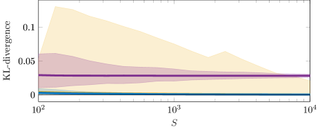
Figure 6: Kullback-Leibler divergence from the density estimate using MCMC to the density estimates using the plain split-normal approximation (purple), IS (yellow), and PSIS (blue). The shaded areas show the envelope of the KL-divergence from all 1000 runs. The variability of the plain split-normal approximation (purple) reduces with increasing number of draws $S$, but the KL-divergence doesn’t decrease. IS (yellow) has the highest variability.

5.2 Importance-sampling leave-one-out cross-validation

We next demonstrate the use of Pareto smoothed importance sampling for leave-one-out (LOO) cross-validation approximation. The $i$th leave-one-out cross-validation predictive density can be approximated with

$$p(\tilde{y}_{i}|y_{-i})\approx\frac{\sum_{s=1}^{S}w_{i}(\theta_{s})p(\tilde{y}_{i}|\theta_{s})}{\sum_{s=1}^{S}w_{i}(\theta_{s})}.$$ (17)

Importance sampling LOO was proposed by Gelfand et al., (1992), but for long time it was not widely used as the estimator is unreliable if the weights have infinite variance. For some simple models, such as linear and generalized linear models with specific priors, it is possible to analytically check the sufficient conditions for the variance of the importance weights in IS-LOO to be finite (Peruggia,, 1997; Epifani et al.,, 2008), but this is not generally possible. Furthermore, even if the variance would be finite, it is possible that the pre-asymptotic behavior is indistinguishable from the infinite variance case as discussed in Section 3.

We first demonstrate properties of IS, TIS, and PSIS with the stack loss data, which is known to have one observation producing infinite variance for LOO importance ratios. Then we demonstrate the speed and reliability of PSIS-LOO for performing model assessment and comparison for predictive regression models for 105 different protein expressions.

LOO for stack loss data.

The stack loss data has $n=21$ daily observations on one response variable and three predictors pertaining to a plant for the oxidation of ammonia to nitric acid. The model is a simple Gaussian linear regression. We fit the model using Stan (Stan Development Team,, 2017); the code is in appendix I. Peruggia, (1997) showed, for a specific choice of prior distributions that we do not recommend to be used in real analyses, that the importance ratios have an infinite variance when leaving out the first data point.

Figure 7 shows the RMSE (compared to the exact LOO) and MCSE estimate (combined error from importance sampling and MCMC as defined in Section 2.2) from 100 runs for the LOO estimated expected log predictive densities $\mathrm{elpd}_{i}=\log p(y_{i}|x_{i},D_{-i})$ and leave-one-out predictive mean $\operatorname{\mathrm{E}}(\mu_{i}|x_{i},D_{-i})$ (where $D_{-i}=(x_{-i},y_{-i})$ denotes the data without $i$th observation) estimated with IS, TIS and PSIS when leaving out the first or 21st observation. Pareto smoothing and MCSE estimates were adjusted based on relative MCMC sample efficiency. The true values were computed by actually leaving out the $i$th observation and using multiple long MCMC chains to get a small Monte Carlo error. PSIS gives the smallest RMSE, and the accuracy of the MCSE estimates are what we would expect based on $h$ specific $\hat{k}$’s: error estimates are accurate for $\hat{k}<0.5$ and optimistic for $\hat{k}>0.7$.

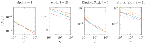
Figure 7: RMSE with IS (yellow), TIS (red) and PSIS (blue), and the MCSE estimates with PSIS (red dashed lines) for the expected log predictive densities $\mathrm{elpd}_{i}=\log p(y_{i}|x_{i},D_{-i})$ and leave-one-out predictive mean $\operatorname{\mathrm{E}}(\mu_{i}|x_{i},D_{-i})$. Average $h$ specific $\hat{k}$’s, using $S=10^{5}$ draws from each of 100 runs, are $0.46,0.79,0.45,0.81$, in the order of subplots.

LOO for 105 protein expression data sets.

We demonstrate the benefit of fast importance sampling leave-one-out cross-validation and PSIS diagnostics with the example of a model for the combined effect of microRNA and mRNA expression on protein expression. The data were published by Aure et al., (2015) and are publicly available; we used the preprocessed data as described by Aittomäki, (2016). Protein, mRNA, and microRNA expression were measured from 283 breast cancer tumor samples, and when predicting the protein expression the corresponding gene expression and 410 microRNA expressions were used. We assumed a multivariate linear model for the effects with a Gaussian prior and used Stan (Stan Development Team,, 2017) to fit the model. Initial analyses gave reason to suspect outlier observations; to verify this, we compared Gaussian and Student-$t$ observation models.

For 4000 posterior draws, the computation for one gene and one model takes about 9 minutes (desktop Intel Xeon CPU E3-1231 v3 @ 3.40GHz x 8), which is reasonable speed. For all 105 genes, the computation takes about 30 hours. Exact regular LOO for all models would take 125 days, and 10-fold cross-validation for all models would take about 5 days. Pareto smoothed importance sampling LOO (PSIS-LOO) took less than one minute for all models. However, we do get several leave-one-out cases where $\hat{k}>0.7$, which we should not trust based on our results above. Figure 8 shows $\hat{k}>0.7$ values for 105 Gaussian and Student-$t$ linear models, where each model may have several leave-one-out cases with $\hat{k}>0.7$. Large $\hat{k}$ values arise when the proposal and the target distributions are very different, which is typical when there are highly influential observations. Switching to the Student-$t$ model reduces the number of high $\hat{k}$ values, as the outliers are less influential if they are far in the tail of the $t$-distribution. When working with many different models, the Stan team has noticed that high $\hat{k}$ values are also a useful indicator that there is something wrong with the data or the model (Gabry et al.,, 2019).

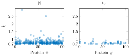
Figure 8: $\hat{k}>0.7$ values for 105 Gaussian and Student-$t$ linear models predicting protein expression levels.

Figure 9 shows the accuracy of PSIS MCSE estimates for the expected log predictive densities with respect to different $\hat{k}$ values (computed only for $\hat{k}>0.5$). True values were computed by actually leaving out the $i$th observation and rerunning MCMC. We can see that $\hat{k}$ is a useful diagnostic and the MCSE estimates are accurate for $\hat{k}<0.7$, as in the simulation experiments, and fail for $\hat{k}\geq 0.7$.

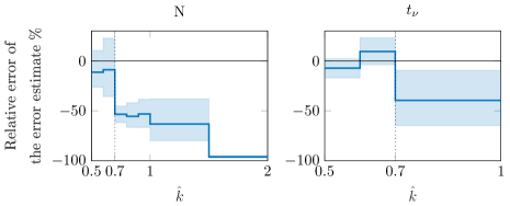
Figure 9: Relative error of the PSIS MCSE estimates. True error was computed as RMSE of expected log predictive density $\mathrm{elpd}_{i}$ estimates with $\hat{k}$ on common interval. Boundaries of intervals can be seen as steps in the plots.

To improve upon PSIS-LOO we can make the exact LOO computations for any points corresponding to $\hat{k}>0.7$ (for which we cannot trust the MCSE estimates). In this example, there were 352 such cases for the Gaussian models and 53 for the Student-$t$ models, and the computation for these took 42 hours. Although combining PSIS-LOO with exact LOO for certain points substantially increases the computation time in this example, it is still less than the time required for 10-fold-CV.

The left subplot in Figure 10 shows comparison of PSIS-LOO and PSIS-LOO+ (PSIS-LOO with exact computation for cases with $\hat{k}>0.7$) when comparing the difference of expected log predictive densities $\sum_{i=1}^{n}\left(\mathrm{elpd}_{i}(t_{\nu})-\mathrm{elpd}_{i}(\operatorname{\mathrm{N}})\right)$. We see that with high $\hat{k}$ values, the error of PSIS-LOO can be large (the error would be large for IS and TIS, too). To trust the model comparison, we recommended using PSIS-LOO+ with exact computation for cases with $\hat{k}>0.7$ or $K$-fold-CV. The right subplot shows the final model comparison results for all 105 models predicting protein expression levels. For most of the proteins, the student-$t$ model is much better, and the Gaussian model is not significantly better for any of the proteins.

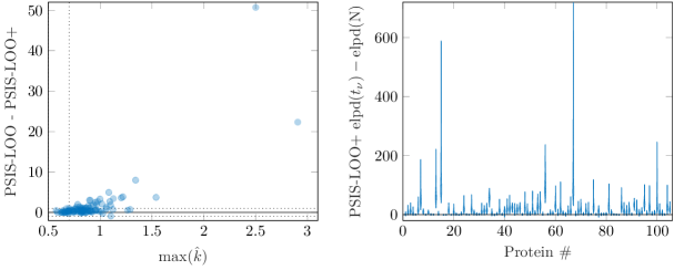
Figure 10: Left plot shows comparison of PSIS-LOO and PSIS-LOO+ (PSIS-LOO with exact computation for cases with $\hat{k}>0.7$) when comparing the difference of expected log predictive densities $\sum_{i=1}^{n}(\mathrm{elpd_{i}(t_{\nu})}-\mathrm{elpd_{i}(\operatorname{\mathrm{N}})})$. Right plot shows the PSIS-LOO+ estimated improvement of expected log predictive densities when switching from Gaussian model to Student-$t$ model.

6 Discussion

Importance weighting is a widely used tool in statistical computation. Even in the modern era of Markov chain Monte Carlo, approximate algorithms are often necessary, in which case we should adjust approximations when possible to better match target distributions. However, a challenge for practical applications of importance weighting is the well known fact that importance-weighted estimates are unstable if the weights have high variance.

In this paper, we have shown that it is possible to reduce the mean square error of importance sampling estimates using a particular stabilizing transformation that we call Pareto smoothed importance sampling (PSIS). The key step is to replace the largest weights by expected quantiles from a generalized Pareto distribution. We have also demonstrated greatly improved Monte Carlo standard error estimates, natural diagnostics for gauging the reliability of the estimates, and empirical convergence rate results that closely follow known theoretical results.

A useful feature of PSIS is the $\hat{k}$ diagnostic, which allows the user to assess the reliability of PSIS:

• If $\hat{k}\leq 0.5$ then PSIS behaves like the importance ratios have finite variance and the resulting estimate will be accurate and converge rate is $S^{-1/2}$.

• If $0.5<\hat{k}\lesssim 0.7$ then the variance is infinite and plain IS can behave poorly. PSIS works well in this regime, but the convergence rate is between $S^{-1/2}$ and $S^{-3/10}$ (worse than cubic root rate, to reduce the variance by $2^{a}$, we need approximately $10^{a}$ more draws)).

• If $0.7\gtrsim\hat{k}$ it quickly becomes too expensive to get an accurate estimate. We do not recommend using PSIS when $\hat{k}\gtrsim 0.7$, although adaptive importance sampling still can be used to improve the proposal distribution.

With these recommendations, PSIS is a reliable, accurate, and trustworthy variant of important sampling that comes with a built-in heuristic that allows it to fail loudly when it becomes unreliable.

Although $\hat{k}$ was originally targeted for self-normalized importance sampling, it can be used to diagnose also ordinary importance sampling and the distribution of any Monte Carlo draws as discussed and demonstrated by some references mentioned in the next section.

6.1 Other examples in the literature

This work has been cited over 200 times since the appearance of the original preprint in 2015 (Vehtari and Gelman,, 2015), and during that time there have been a number of extensions and applications proposed in the literature. In this section, we highlight a few of the main ones.

First, there was a suite of works that investigated the use of PSIS for computing cross-validation scores. Vehtari et al., (2017) provide additional comparisons between IS-LOO, TIS-LOO, PSIS-LOO, and widely applicable information criterion (Watanabe,, 2010). Vehtari et al., (2016) use PSIS-LOO to improve integrated importance sampling in case of Gaussian process models with non-Gaussian observation models. Bürkner et al., 2020b use PSIS-LOO for Bayesian non-factorized multivariate normal and Student-$t$ models. Magnusson et al., (2019, 2020) apply PSIS-LOO in case of variational and Laplace approximations to posteriors. Bürkner et al., 2020a apply PSIS in leave-future-out cross-validation for time series, where the proposal distribution is conditioned on fewer data and thus by construction tend to have thicker tails than the target distribution, but with a large number of steps in time, eventually new MCMC posterior computation is needed. Fong and Holmes, (2021) comment how PSIS could improve add-one-in importance sampling for conformal Bayesian computation. While in leave-future-out cross-validation several future observations are included to update the posterior, in add-one-in importance-sampling one of the existing observations is included again to update the posterior.

Second, there has been work using PSIS as a building block to improve Bayesian models and workflow. Yao et al., 2018a ; Yao et al., (2021, 2022) use PSIS-LOO for Bayesian stacking, which is a form of model combination common in machine learning, and for its extensions to hierarchical stacking and stacking of non-mixing MCMC chains. Piironen et al., (2020) use PSIS-LOO as part of projection predictive variable selection to speed-up the selection of the number of variables to include. McCartan, (2021) uses PSIS for prior sensitivity analysis, and Kallioinen et al., (2021) use PSIS and iterative moment matching PSIS (Paananen et al.,, 2021) for diagnosing both prior and likelihood sensitivity.

Third, the $\hat{k}$ diagnostic has been used to compare variational posterior approximations, for example, by Yao et al., 2018b , Dhaka et al., (2021), and Zhang et al., (2021).

Finally, $\hat{k}$ can be used to diagnose any Monte Carlo estimate. Dhaka et al., (2020) use $\hat{k}$ to diagnose number of finite fractional moments of stochastic optimization in approximate convergence. Paananen et al., (2021) discuss and demonstrate that Pareto $\hat{k}$ is useful for any Monte Carlo expectation estimate to diagnose whether the sampled distribution has tail with $\hat{k}<0.7$. Dhaka et al., (2021) use $\hat{k}$ to diagnose the behavior of Monte Carlo estimates of commonly used divergences in variational inference.

6.2 Other weight transformations

Truncated weights has been studied also by Koblents and Míguez, (2015), who use condition $M/S\rightarrow 0$ in the asymptotic proofs, but in practice recommend to set $M=S/10$. This approach is likely to have similar bias as TIS by Ionides, (2008), as the difference is just in the rule to choose the truncation point.

Míguez, (2017) propose to set the largest weights above some quantile to the average of those weights. This reduces the bias compared to the simple truncation. This approach keeps the average of all weights the same, so it has a smaller bias than TIS (given a similar truncation rule). Compared to PSIS, this approach is likely to (a) have higher variance as the highest weight can still have a big influence on the average of the largest weights, (b) have higher bias as on expectation the smallest of the transformed weights are overweighted and largest of the transformed weights are underweighted, and (c) be more sensitive to the threshold as the largest non-transformed weight and smallest transformed weight are made more different.

Martino et al., (2018) compare the methods by Koblents and Míguez, (2015) and Míguez, (2017). They state that condition $M\leq\sqrt{S}$ is useful for the asymptotic results, but in the experiments set $M=S/5$.

6.3 Moving beyond PSIS

Multiple and adaptive importance sampling.

Pareto $\hat{k}$ can be used to compare proposal distributions both in single and multiple importance sampling (for a review of multiple IS, see Elvira et al.,, 2019), and as a diagnostic in adaptive importance sampling (for a review of adaptive IS, see Bugallo et al.,, 2017). Sometimes it can be possible to choose a proposal distribution that guarantees finite variance of importance weights (see, e.g., Owen and Zhou,, 2000), but this doesn’t guarantee useful pre-asymptotic convergence rate as shown in Section 3.3.

In Section 5.1 we demonstrated use of $\hat{k}$ to compare simple normal and split-normal proposal distributions. Dhaka et al., (2021) use $\hat{k}$ diagnostic to compare normal, Student-$t$, planar flow (Rezende and Mohamed,, 2015) and NVP flow (Dinh et al.,, 2017) variational approximations in low and high dimensions.

Bürkner et al., 2020a use $\hat{k}$ diagnostic to choose regeneration steps in sequential importance sampling for leave-future-out cross-validation, and demonstrate also that the proposal distributions are in general better when adding observations than when removing observations, leading to a smaller number of regeneration refits.

Paananen et al., (2021) use $\hat{k}$ diagnostic as part of the implicitly adaptive multiple importance sampling approach to decide when the iterative adaptation can be stopped and thus minimizing the computational cost. Yao et al., (2020) use $\hat{k}$ diagnostic as part of the adaptive path sampling algorithm to decide whether further adaptation of the pseudo-prior is required.

In all these examples, PSIS was also used to smooth the weights and improve the final importance sampling estimates.

An anonymous reviewer suggested that $\hat{k}$ could be used also as a diagnostic tool to decide which weighting schemes (see Elvira et al.,, 2019) are better, or to select the operation point in the tradeoff between variance reduction in the weights and computational complexity; see Elvira et al., (2015).

Population Monte Carlo and particle filters.

PSIS is especially useful when one proposal distribution or its computationally cheap transformation can be used for several slightly different target distributions, as in leave-one-out (Vehtari et al.,, 2017) and leave-future-out cross-validation (Bürkner et al., 2020a, ). In leave-future-out cross-validation, the observations are added sequentially, and the posterior approximation is updated using importance weighting until $\hat{k}>0.7$ and then the posterior sample is regenerated with MCMC. This resembles the algorithms such as population and sequential Monte Carlo, and particle filtering (see, e.g., Cappé et al.,, 2004; Crisan and Rozovskii,, 2011, part 8).

Koblents and Míguez, (2015) and Míguez, (2017) demonstrate the benefit of variants of truncated importance sampling in population Monte Carlo, and it can be assumed that PSIS would further improve the results. Senarathne et al., (2020) use PSIS to stabilize a Laplace-based sequential Monte Carlo algorithm for adaptive design of experiments.

It can also be expected that variance of particle filter estimates in filtering and smoothing problems could be reduced with Pareto smoothing of the weights and with improved regeneration control by using Pareto $\hat{k}$ diagnostic. Analyzing the effect of these in different population and sequential Monte Carlo and particle filter algorithms and applications would be worthy of further study.

Appendix A Scaling of distribution of mean of truncated means

PSIS replaces the $M$ largest weights with the expected ordered statistics of Pareto distribution. The generalized central limit theorem states that the largest expected ordered statistic scales as $S^{k}$ (see, e.g. Bouchaud and Georges,, 1990, p. 138), and we can model the distribution of the mean of the expected ordered statistics as mean of truncated Pareto variables. Zaliapin et al., (2005) provide equations for mean and variance of truncated Pareto distribution:

$$\mu_{y}=\operatorname{\mathrm{E}}\left(X_{1}\mid X_{1}\leq y\right)=\begin{cases}\frac{1}{k-1}\left(y^{1-{1/k}}-1\right)/\left(1-y^{-{1/k}}\right),&\qquad k\neq 1,\\ \log(y)/\left(1-y^{-1}\right),&\qquad k=1,\end{cases}$$

$$\sigma_{y}^{2}=\operatorname{\mathrm{Var}}\left(X_{1}\mid X_{1}\leq y\right)=\begin{cases}\frac{1}{2k-1}\left(y^{2-{1/k}}-1\right)/\left(1-y^{-{1/k}}\right)-\mu_{y}^{2},&k\neq 0.5,\\ 2\log(y)/\left(1-y^{-2}\right)-\mu_{y}^{2},&k=0.5.\end{cases}$$

We set the truncation point to the largest expected order statistic, $y=S^{k}$, and get

$$\mu_{y}=\operatorname{\mathrm{E}}\left(X_{1}\mid X_{1}\leq S^{k}\right)=\begin{cases}\frac{1}{k-1}\left(S^{k-1}-1\right)/\left(1-S^{-1}\right),&\qquad k\neq 1,\\ \frac{1}{2}\log(S)/\left(1-S^{-1}\right),&\qquad k=1,\end{cases}$$

$$\sigma_{y}^{2}=\operatorname{\mathrm{Var}}\left(X_{1}\mid X_{1}\leq S^{k}\right)=\begin{cases}\frac{1}{2k-1}\left(S^{2k-1}-1\right)/\left(1-S^{-1}\right)-\mu_{y}^{2},&k\neq 0.5,\\ \log(S)/\left(1-S^{-1}\right)-\mu_{y}^{2},&k=0.5.\end{cases}$$

When $S$ is big and $k\in(0,0.5-0.5/\log_{10}(S))$, the RMSE is dominated by the variance, $\sigma_{y}^{2}$ is dominated by $\operatorname{\mathrm{E}}(X_{1}^{2})$, and

$$\left(S^{2k-1}-1\right)/\left(S^{-1}-1\right)\in(0.9,1).$$

Thus the effect of $k$ is small for $\sigma_{y}^{2}$, and the standard deviation of mean of Pareto truncated variables then scales approximately as $S^{-1/2}$ matching CLT scaling (the standard deviation can still depend on $k$). Interestingly, the above threshold ($0.5-0.5/\log_{10}(S)$) is equal to half of the max $\hat{k}$ threshold given $S$ (see Section 3.2.4). The scale rate change around this threshold is smooth and threshold is not describing a sharp phase transition.

When $S$ is big and $k=0.5$, the variance dominates bias, the RMSE is dominated by the variance, $\sigma_{y}^{2}$ is dominated by $\operatorname{\mathrm{E}}(X_{1}^{2})$, and

$$\log(S)/\left(1-S^{-1}\right)\approx\log(S).$$

Thus the standard deviation of mean of Pareto truncated variables scales approximately as $(S/\log(S))^{-1/2}$, matching the GCLT scaling (at $k=0.5$).

When $S$ is big and $k\in(0.5+0.5/\log_{10}(S),1)$, we need to consider the effect of both bias and variance for RMSE. Bias is

$$\mu(\left(1-S^{k-1}\right)/\left(1-S^{-1}\right)-1) \approx\mu S^{k-1}.$$

$\sigma_{y}^{2}$ is dominated by $\operatorname{\mathrm{E}}(X_{1}^{2})$, and

$$\left(S^{2k-1}-1\right)/\left(1-S^{-1}\right) \approx S^{2k-1}.$$

The standard deviation of mean of truncated Pareto variables scales then approximately as $(S^{2k-1})^{1/2}S^{-1/2}=S^{k-1}$. Both bias and standard deviation of mean scale as $S^{k-1}$, so RMSE scales also as $S^{k-1}$. The additional terms, which depend on $k$, make the bias to grow faster than the standard deviation, and thus eventually when $k$ is big enough—approximately $0.7$—RMSE is dominated by the bias; see also Section 3.2.3.

The behavior of scaling of mean of truncated Pareto variables varies smoothly with $k$, but approximately we have CLT scaling $S^{-1/2}$ when $k\in(0,0.5-0.5/\log_{10}(S))$ and GCLT scaling $S^{k-1}$ when $k\in(0.5+0.5/\log_{10}(S),1)$, between these the scaling changes smoothly and monotonically so that it is $(S/\log(S))^{-1/2}$ when $k=0.5$. When $S$ increases, the range $k\in(0.5-0.5/\log_{10}(S),0.5+0.5/\log_{10}(S))$ gets shorter.

The above equations are approximate as for simplicity we have dropped minor terms, and they do not take into account 1) the reduced variance of PSIS due to replacing $M$ largest weights with expected ordered statistics, and 2) the difference in bias between analytic integral and use of (approximated) expected ordered statistics. Based on the experiments these differences do not affect the order of the scaling.

For self-normalized truncated importance sampling (TIS), the truncation point is $y=\bar{r}S^{1/2}$, where $\bar{r}=\frac{1}{S}\sum_{s=1}^{S}r_{s}$ (Ionides,, 2008, Appendix B). This truncation level tends to be lower than truncation in TIS, which reduces the variance, but increases bias. Analyzing the effect of $\bar{r}$ is complicated as it has infinite variance. When $k<1$ the truncated mean is

$$\frac{1}{k-1}\left(cS^{1/2-1/(2k)}-1\right)/\left(1-cS^{-1/(2k)}\right).$$

When $S$ is big and $0.5\ll k<1$,

$$\left(cS^{1/2-1/(2k)}-1\right)/\left(1-cS^{-1/(2k)}\right)\approx\left(cS^{1/2-1/(2k)}-1\right),$$

and TIS bias scales as $cS^{1/2-1/(2k)}$ and thus grows faster than PSIS bias. Here $c$ includes the effect of $\bar{r}$ which depends on the observed ratios. Specifically, this truncation fails sometimes when there is one extremely large weight that causes the truncation level to rise so high that other large weights are not truncated (demonstrated in the examples).

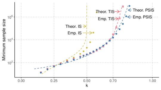
Figure 11: Theoretical (dashed lines) and empirical (dots) minimum sample size to control RMSE for PSIS, TIS, and IS as a function of $k$. Empirical results are obtained with 10 000 repeated simulations, using grid of $k$ and $S$ values and interpolation, to find the sample sizes needed to obtain RMSE of $0.05$.

Figure 11 shows the theoretical and empirical minimum sample sizes for PSIS, TIS, and IS. Theoretically IS has infinite variance when $k>0.5$, but the empirical RMSE result for IS is optimistic as the error distribution has a thick tail, and with finite number of repeated simulations that tail is not well explored. This optimism means also that when $k$ is close to $0.5$ or larger, IS with finite number of draws is not unbiased. The empirical behavior of RMSE IS depends both on the sample size $S$, but also on the number of repeated simulations. TIS has similar RMSE as PSIS until approximately $k>0.65$, but the RMSE of TIS is dominated by the bias much earlier and thus variance based MCSE estimates are less useful for TIS than for PSIS. See more discussion in Section 3.2.3.

Appendix B Relative convergence rates

When $k<0.5-0.5/\log_{10}(S)$, the root mean squared error of PSIS scales approximately as $S^{-1/2}$ as under CLT. If we write this as $(S^{-1/2})^{\alpha},\alpha=1$, we can then consider relative convergence rates $\alpha$ compared to the CLT rate. For $k\in(0.5+0.5/\log_{10}(S),1)$, $(S^{-1/2})^{\alpha}=S^{(k-1)}$ is solved by $\alpha=2-2k$. When $k=0.5$,

$$(S^{-1/2})^{\alpha} =(S/\log(S))^{-1/2}$$

$$S^{\alpha} =(S/\log(S)) |\ \log$$

$$\alpha\log(S) =\log(S/\log(S)) |\ \frac{d}{dS}$$

$$\alpha/S =(1-1/\log(S))/S$$

$$\alpha =1-1/\log(S).$$

The above simple equations help to provide insight to the behavior of relative convergence rate for $k\ll 0.5$, $k=0.5$, and $k\gg 0.5$. We can also derive more accurate smooth approximation from $\operatorname{\mathrm{E}}[X_{1}^{2}]$ of truncated Pareto mean (see Appendix A) and get relative convergence rate

$$\begin{cases}\frac{2(k-1)S^{(2k+1)}+(1-2k)S^{(2k)}+S^{2}}{(S-1)(S-S^{(2k)})},&k\neq 0.5,\\ 1-1/\log(S),&k=0.5,\end{cases}$$

which can be used as part of computer assisted diagnostics.

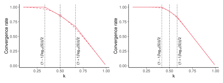
Figure 12: Convergence rate as a function of $k$ and $S$. Red solid line shows a piecewise linear approximation and Red dashed line shows a smooth approximation. Both approximations are based on properties of distribution of mean of truncated Pareto variables (see text). Left subplot shows the result with $S=10^{3}$ and the right plot shows the result with $S=10^{6}$. The dotted lines show the approximate thresholds used for the piecewise linear approximation. Empirical results are obtained from 10 000 repeated simulations.

Figure 12 shows a piecewise linear and smooth approximations of the relative convergence rate when $S=10^{3}$ and $S=10^{6}$. Figure 4 in Section 3.2.6 shows the relative convergence rate approximation (smooth) and empirical results when $S=10^{4}$. These convergence rate approximations match well the empirical results in Figures 18, 23, and 26, except in the fourth subplot of Figure 23. In that case, the actual convergence rate for first and second moment is better than predicted by $h$-specific $\hat{k}_{h}$. This is explained by having a bounded ratio distribution, and initially not observing ratios near the bound, but when the sample size increases the bound starts to have an effect and convergence is faster than initially predicted (see also Section 3.2.9).

When $k=0.5$ and $S\rightarrow\infty$, the convergence rate approaches $1$, but with any finite $S$ the convergence rate is less than $1$.

Appendix C Proof of Theorem 1

We can write the PSIS estimator as a Winsorized version of the truncated estimator of Ionides, (2008) plus an extra bias correction term:

$$I^{S}_{h}=\frac{1}{S}\sum_{s=1}^{S}\left(r(\theta_{s})\wedge r_{(S-M+1):S}\right)h(\theta_{s})\,+\,\frac{1}{S}\sum_{j=1}^{M}w^{+}_{j}h(\theta_{S-M+j}).$$

For truncated importance sampling, the number of draws, $M$, that exceed the threshold is random while the threshold is fixed. For the Winsorized version the number of exceedences is fixed but the threshold is random. The threshold is the $M$th largest value of $r_{s}$. We denote this using order statistics notation: we reorder the sample so that

$$r_{1:S}\leq r_{2:S}\leq\dots r_{S:S}.$$

With this notation, the threshold is $T=r_{S-M+1:S}$ and the Winsorized importance sampler (WIS) is

$$I^{S}_{\text{WIS}}=\frac{1}{S}\sum_{s=1}^{S-M}h_{s:S}r_{s:S}+\frac{r_{S-M+1:S}}{S}\sum_{s=S-M+1}^{S}h_{s:S},$$

where $(r_{s:S},h_{s:S})$ are the $(r_{s},h_{s})$ pairs ordered so that $r_{1:S}\leq r_{2:S}\leq\dots\leq r_{S:S}$.

Conditioning on the event $r_{S-M+1:S}=T$ yields,

$$\mathbb{E}\left(I_{\text{WIS}}^{S}\mid r_{S-M+1:S}=T\right)=\left(1-\frac{M}{S}\right)\mathbb{E}(RH\mid R<T)+\frac{MT}{S}\mathbb{E}(H\mid R\geq T).$$

From this, the bias, conditional on $r_{S-M+1:S}=T$, is

$$\left|I-\mathbb{E}\left(I_{\text{WIS}}^{S}\mid r_{S-M+1:S}=T\right)\right|=\left|\left(\Pr(R<T)-\left(1-\frac{M}{S}\right)\right)\mathbb{E}(RH\mid R<T)\right.\\ \left.+\left[\Pr(R\geq T)-\frac{M}{S}\right]\mathbb{E}(H(R-T)\mid R\geq T)\right|.$$

Using the triangle inequality

$$\left|\mathbb{E}(RH\mid R>T)\right|\leq\frac{\mathbb{E}(R|H|1(R<T))}{\Pr(R<T)}\leq\frac{\|h\|_{L^{1}(p)}}{\Pr(R<T)}$$

we see that the first term in the bias can be bounded if we can bound the relative error,

$$\mathbb{E}\left|1-\frac{1-M/S}{\Pr(R<r_{S-M+1:S})}\right|.$$

To attack this expectation, we use the following lemma that derives the distribution of the relative error we incur when approximating $\Pr(R>r_{S-M+1:S})$ with $1-M/S$.

Lemma 1.

Let $x_{s}$, $s=1,\ldots S$ be an iid sample from $F_{X}$, and let $r\in[0,S]$ be an integer. Then, for any $p\in(0,1)$,

$$\frac{p}{F_{X}(x_{r:S})}-p\stackrel{{\scriptstyle d}}{{=}}\frac{p(S-r+1)}{r}\mathcal{F},$$

and

$$\frac{1-p}{1-F_{x}/(x_{r:S})}-(1-p)\stackrel{{\scriptstyle d}}{{=}}\frac{k(1-p)}{S-r+1}\mathcal{F}^{-1},$$

where $\mathcal{F}$ is an F-distributed random variable with parameters $(2(S-k+1),2k)$.

Proof.

For any $t\geq 0$,

$$\Pr\left(\frac{p}{F_{X}(x_{k:S})}-p\leq t\right) =\Pr\left(p-pF_{X}(x_{k:S})\leq tF_{X}(x_{k:S})\right)$$

$$=\Pr\left(p\leq(t+p)F_{X}(x_{k:S})\right)$$

$$=\Pr\left(F_{X}(x_{k:S})\geq\frac{p}{p+t}\right)$$

$$=\Pr\left(x_{k:S}\geq F_{X}^{-1}\left(\frac{p}{p+t}\right)\right)$$

$$=1-I_{\frac{p}{p+t}}(k,S-k+1)$$

$$=I_{\frac{t}{p+t}}(S-k+1,k),$$

where $I_{p}(a,b)$ is the incomplete beta function; see equation 2.1.5 in David and Nagaraja, (2004). ∎

It follows then that

$$\left|1-\frac{1-M/S}{R(r_{S-M+1})}\right|\stackrel{{\scriptstyle d}}{{=}}\left|\frac{M}{S}-\frac{M(S-M)}{S(S-M-1)}\mathcal{F}\right|\leq\frac{M}{S}+\frac{M(S-M)}{S(S-M-1)}\mathcal{F},$$

where $\mathcal{F}$ has an F-distribution with $(M,S-M+1)$ degrees of freedom. As $\mathbb{E}(\mathcal{F})=1+1/(S-M-1)$, it follows that this term goes to zero as long as $M=o(S)$. This shows that the first term in the bias goes to zero.

The second term in the bias is

$$\left(\Pr(R\geq T)-\frac{M}{S}\right)\mathbb{E}(H(R-T)\mid R\geq T).$$

As before, we can write this as

$$\left(1-\frac{M/S}{1-R(T)}\right)|\mathbb{E}(H(R-T)1_{R\geq T})|\leq\left|1-\frac{M/S}{1-R(T)}\right|\|h\|_{L^{1}(p)}.$$

By our lemma, we know that the distribution of the term in the absolute value when $T=r_{S-M+1}$ is the same as

$$1-\frac{M}{S}-\left(1-\frac{M}{S}+\frac{1}{S}\right)\mathcal{F}=(\mu_{F}-\mathcal{F})+\frac{M}{S}(\mathcal{F}-\mu_{F})-\frac{1}{S}\mathcal{F}+\frac{1}{M-1}\left(\frac{M}{S}-1\right),$$

where $\mathcal{F}\sim\text{F}_{2(S-M+1),2M}$, which has mean $\mu_{F}=1+(M-1)^{-1}$ and variance

$$\sigma^{2}_{F}=\frac{M^{2}S}{(S-M+1)(M-1)^{2}(M-2)}=\frac{1}{M}\left(1+\mathcal{O}(M^{-1}+MS^{-1})\right).$$

From Jensen’s inequality, we get

$$\mathbb{E}(|\mathcal{F}-\mu_{F}|)\leq\sigma_{F}=M^{-1/2}(1+o(1)).$$

If follows that

$$\mathbb{E}\left|1-\frac{M/S}{1-R(r_{S-M+1:S})}\right|\leq M^{-1/2}(1+o(1))M^{1/2}S^{-1}(1+o(1))+S^{-1}(1+o(1))+(M-1)^{-1}(1+o(1)),$$

and so we get vanishing bias as long as $M\rightarrow\infty$ and $M/S\rightarrow 0$.

Theorem 2.

Let $\theta_{s}$, $s=1,\ldots,S$ be an iid sample from $G$ and let $r_{s}=r(\theta_{s})\sim R$. Assume that

1. $R$ is absolutely continuous

2. $M\rightarrow\infty$ and $S^{-1}M\rightarrow 0$

3. $h\in L^{1}(p)$

Then the Winsorized importance sampling converges in $L^{1}$ and is asymptotically unbiased.

Assuming that $R-T\mid R\geq T$ is in the domain of attraction of a generalized Pareto distribution with shape parameter $k$. A sufficient condition, due to von Mises, is that

$$\lim_{r\rightarrow\infty}\frac{rR^{\prime}(r)}{1-R(r)}=\frac{1}{k}.$$

This is basically a regularity condition at infinity. For example if $1-R(r)$ is regularly varying at infinity and $R^{\prime}(r)$ is, eventually, monotone decreasing, then this condition holds.

The von Mises condition is natural here, as Falk and Marohn, (1993) show that the relative error from approximating the tail of $R$ by a generalized Pareto density is the same as the relative error in the von Mises condition. That is, if

$$\frac{rR^{\prime}(r)}{1-R(r)}=\frac{1}{k}(1+\mathcal{O}(r^{-\alpha}))$$

then

$$R^{\prime}(r)=cw(cr-d)(1+\mathcal{O}(r^{-\alpha})),$$

where $c$ and $d$ are constants and $w$ is the density of a generalized Pareto distribution.

Under those two assumptions, we can swap out the density of $(R-T)\mid R>T$ with its asymptotic approximation and get that, conditional on $T=r_{S-M+1:S}$,

$$\mathbb{E}(H(R-T)\mid R>T)=(k-1)^{-1}T.$$

Hence, the second term in the bias goes to zero if

$$\mathbb{E}\left(r_{S-M+1:S}\left(1-R(r_{s-M+1:S})-\frac{M}{S}\right)\right)$$

goes to zero.

This helps us understand that even if a distribution doesn’t have finite moments, away from the extremes its order statistics always do. This means that we can use Cauchy-Schwartz to get

$$\left|\mathbb{E}\left(r_{S-M+1:S}\left(1-R(r_{s-M+1:S})-\frac{M}{S}\right)\right)\right|\leq\mathbb{E}\left(r_{S-M+1:S}^{2}\right)^{1/2}\mathbb{E}\left(\left(1-R(r_{s-M+1:S})-\frac{M}{S}\right)^{2}\right)^{1/2}.$$

Leaning into a result by Bickel, (1967) and fixing a typo there, we get that

$$\mathbb{E}(r_{k:M}^{2})\leq Ck\begin{pmatrix}S\\ k\end{pmatrix}\int_{0}^{1}t^{k-2-1}(1-t)^{S-k-2}\,dt.$$

Noting that $B(n,m)=\Gamma(n)\Gamma(m)/\Gamma(n+m)$, we can rewrite the upper bound in terms of the beta function to get

$$\mathbb{E}(r_{k:M}^{2})\leq C\frac{\Gamma(S+1)}{\Gamma(S-3)}\frac{\Gamma(k-2)}{\Gamma(k+1)}\frac{\Gamma(S-k-1)}{\Gamma(S-k+1)}.$$

To show that this doesn’t grow too quickly, we use the identity

$$\frac{\Gamma(x+a)}{\Gamma(x+b)}\propto x^{a-b}(1+\mathcal{O}(x^{-1})),$$

from which it follows that

$$\mathbb{E}(r_{k:M}^{2})\leq CS^{4}k^{-3}(S-k)^{-2}(1+\mathcal{O}(S^{-1}))(1+\mathcal{O}(k^{-1}))(1+\mathcal{O}((S+k)^{-1})).$$

In this case, we are interested in $k=S-M+1$, so

$$\mathbb{E}(r_{k:M}^{2})\leq CS^{4}S^{-3}M^{-2}(1-M/S+1/S)^{-3}(1-1/M)^{-2}(1+\mathcal{O}(S^{-1}))(1+\mathcal{O}(S^{-1}))(1+\mathcal{O}(M^{-1})).$$

Hence $\mathbb{E}(r_{k:M}^{2})=\mathcal{O}(SM^{-2})$. This is increasing in $S$, but we will see that it is not going up too fast.

For the second half, we attack

$$\mathbb{E}\left(\left(1-R(r_{s-M+1:S})-\frac{M}{S}\right)^{2}\right)=\mathbb{E}\left(\left(1-R(r_{s-M+1:S})\right)^{2}-2\left(1-R(r_{s-M+1:S})\right)\frac{M}{S}+\left(\frac{M}{S}\right)^{2}\right).$$

A standard result from extreme value theory is that $R(r_{k:S})$ has the same distribution as the $k$th order statistics from a sample of $S$ independent $\text{uniform}(0,1)$ random variables. Hence,

$$R(r_{S-M+1:S})\sim\text{beta}(S-M+1,M).$$

If follows that

$$\mathbb{E}(1-R(r_{S-M+1:S}))=\frac{M}{S+1}=\frac{M}{S}\frac{1}{1+S^{-1}}$$

and

$$\mathbb{E}((1-R(r_{S-M+1:S}))^{2})=\frac{M(M+1)}{(S+1)(S+2)}=\frac{M^{2}}{S^{2}}\left(\frac{1+M^{-1}}{1+3S^{-1}+2S^{-2}}\right).$$

Adding these and doing asymptotic expansions yields,

$$\mathbb{E}\left(\left(1-R(r_{s-M+1:S})-\frac{M}{S}\right)^{2}\right)=\frac{M^{2}}{S^{2}}+\mathcal{O}\left(\frac{M}{S^{2}}\right),$$

which goes to zero like $\mathcal{O}(S^{-1})$ if $M=\mathcal{O}(S^{1/2})$.

We can multiply this rate together and get that the second term in the bias is bounded above by

$$\left[\left(\frac{S}{M^{2}}(1+\mathcal{O}(M^{-1}+MS^{-1}))\right)\left(\frac{M^{2}}{S^{2}}(1+\mathcal{O}(M^{-1}+MS^{-1})\right)\right]^{1/2}=S^{-1/2}(1+o(1)).$$

Putting all of this together we have proved the following corollary.

Corollary 1.

Let $\theta_{s}$, $s=1,\ldots,S$ be an iid sample from $G$ and let $r_{s}=r(\theta_{s})\sim R$. Assume that

1. $R$ is absolutely continuous and satisfies the von Mises condition

   $$\frac{rR^{\prime}(r)}{1-R(r)}=\frac{1}{k}(1+\mathcal{O}(r^{-1})).$$

2. $M=o(S)$.

3. $h$ is bounded.

Then Winsorized importance sampling converges in $L^{1}$ with rate of, at most, $\mathcal{O}(MS^{-1}+S^{-1/2})$, which is balanced when $M=\mathcal{O}(S^{1/2})$. Hence, WIS is $\sqrt{n}$-consistent.

To tackle the variance part we use

$$\mathbb{V}\left(I_{\text{WIS}}^{S}\right)\leq\mathbb{E}\left([I_{\text{WIS}}^{S}]^{2}\right),$$

noting that we can write $I_{\text{WIS}}^{S}$ compactly as

$$I_{\text{WIS}}^{S}=\frac{1}{S}\sum_{s=1}^{S}h(\theta_{s})\min\{r(\theta_{s}),r_{S-M+1:S}\}.$$

Hence,

$$\mathbb{E}\left([I_{\text{WIS}}^{S}]^{2}\right) =\mathbb{E}_{T\sim r_{S-M+1:S}}\left[\mathbb{E}\left([I_{\text{WIS}}^{S}]^{2}\mid r_{S-M+1:S}=T\right)\right]$$

$$=\frac{1}{S^{2}}\mathbb{E}_{T\sim r_{S-M+1:S}}\left[\mathbb{E}\left(H^{2}\min\{R^{2},T^{2}\}\mid r_{S-M+1:S}=T\right)\right]$$

$$\leq\frac{1}{S^{2}}\mathbb{E}_{T\sim r_{S-M+1:S}}\left[\mathbb{E}\left(RTH^{2}\mid r_{S-M+1:S}=T\right)\right]$$

$$\leq\frac{1}{S^{2}}\mathbb{E}_{T\sim r_{S-M+1:S}}\left[T\|h\|_{L^{2}(p)}^{2}\right],$$

Which goes to zero as long as $\mathbb{E}(r_{S-M+1:S})=o(S^{2})$.

Bickel, (1967) shows that, noting that $\mathbb{E}(R)<\infty$,

$$\mathbb{E}(r_{S-M+1:S})\leq C(S-M+1)\frac{\Gamma(S+1)\Gamma(S-M+1-1)\Gamma(M)}{\Gamma(S-M+1+1)\Gamma(M+1)\Gamma(S-1)}=\frac{S}{M}(1+o(1)),$$

and so the variance is bounded.

The previous argument shows that the variance is $\mathcal{O}(M^{-1}S^{-1})$. We can refine that if we assume the von Mises condition hold. In that case we know that $R(r)=1-cr^{-1/k}+o(1)$ as $r\rightarrow\infty$ and therefore

$$R\left(R^{-1}\left(1-\frac{M}{S}\right)\right) =1-\frac{M}{S+1}$$

$$1-cR^{-1}\left(1-\frac{M}{S+1}\right)^{-1/k}(1+o(1)) =1-\frac{M}{S+1}$$

$$R^{-1}\left(1-\frac{M}{S+1}\right) =c^{-k}\left(\frac{M}{S+1}\right)^{-k}(1+o(1)).$$

Bickel, (1967) shows that $\mathbb{E}(r_{k:S})=R^{-1}(1-M/(S+1))+o(1)$, so combining this with the previous result gives a variance of $\mathcal{O}((M/S)^{k-2})$. If we take $M=\mathcal{O}(S^{1/2})$, this gives $\mathcal{S}^{k/2-1}$, which is smaller than the previous bound for $k<1$. Hence the variance goes to zero and we have proved the following theorem.

Theorem 3.

Let $\theta_{s}$, $s=1,\ldots,S$ be an iid sample from $G$ and let $r_{s}=r(\theta_{s})\sim R$. Assume that

1. $R$ is absolutely continuous

2. $M\rightarrow\infty$ and $M^{-1}S\rightarrow 0$

3. $h\in L^{2}(p)$.

The variance in Winsorized importance sampling is at most $\mathcal{O}(M^{-1}S)$.

Next we look at the PSIS bias correction. Essentially, it works by noting that approximating

$$(1-R(r_{S-M+1:S}))\mathbb{E}(HR\mid R>r_{S-M+1:S})\approx\frac{1}{S}\sum_{m=1}^{M}w_{m}h_{S-M+m:S},$$

where $w_{m}$ is the median $m$th order statistic in an iid sample of $M$ generalized Pareto random variables with tail parameters fitted to the distribution. This is equivalent to a quadrature rule. To see that, we can write

$$\mathbb{E}(HR\mid R>T)=\mathbb{E}(R\,\mathbb{E}(H\mid R)).$$

If we approximate the distribution of $R>T$ by

$$\tilde{R}_{\text{PSIS}}(r)=\frac{1}{M}\sum_{m=1}^{M}1(w_{m}<r)$$

and approximate the conditional probability by

$$\Pr(H<h\mid R=w_{m})\approx 1(h_{S-M+m:S}<h),$$

then the convergence and vanishing variance still holds. To see this, we note that

$$w_{m}=r_{S-M+1}+k^{-1}\sigma\left(\left(1-\frac{j-1/2}{M}\right)^{-k}-1\right).$$

So we are just reweighting our tail $H$ samples by

$$1+\frac{\sigma}{kr_{S-M+1:S}}\left(\left(1-\frac{j-1/2}{M}\right)^{-k}-1\right).$$

Recalling that when $R(r)=1-cr^{-1/k}(1+o(1))$, we had $\sigma=\mathcal{O}(r_{S-M+1:S})$, this term is at most $\mathcal{O}(1+M^{-k})$. This will not trouble either of our convergence proofs.

This leads to the following modification of our previous result, which was stated in Section 4, but repeated here for convenience.

Theorem 1.

Let $\theta_{s}$, $s=1,\ldots,S$ be an iid sample from $G$ and let $r_{s}=r(\theta_{s})\sim R$. Assume that

1. $R$ is absolutely continuous.

2. $M=\mathcal{O}(S^{1/2})$

3. $h\in L^{2}(p)$

4. $k$ and $\sigma$ are known with $\sigma=\mathcal{O}(r_{S-M+1:S})$.

Then Pareto smoothed importance sampling converges in $L^{1}$ and its variance goes to zero and it is consistent and asymptotically unbiased.

In addition, we have the following corollary.

Corollary 2.

Assume further that

1. R satisfies the von Mises condition

   $$\frac{rR^{\prime}(r)}{1-R(r)}=\frac{1}{k}(1+\mathcal{O}(r^{-1})).$$

2. $h$ is bounded.

Then the $L^{1}$ convergence occurs at a rate of, at most, $\mathcal{O}(S^{-1/2})$. Furthermore, the variance of the PSIS estimator goes to zero at least as fast as $\mathcal{O}(S^{k/2-1})$.

Hence, under these additional conditions PSIS is $\sqrt{n}$-consistent.

Appendix D Simulated examples

In the following experiments, we know the true target value and vary the proposal distribution. This allows us to study how $\hat{k}$ functions as a diagnostic and how bad the approximating distribution has to be before the importance sampling estimates and corresponding variance based Monte Carlo standard error (MCSE) estimates defined in Section 2.2 break down. To diagnose the performance with respect to the number of draws $S$, in each of the examples we vary the number of draws from $S=10^{2}$ to $S=10^{5}$. We examine the estimates for the normalization term (zeroth moment), which also has a special role in the importance sampling examples, and estimates for $\operatorname{\mathrm{E}}(h(\theta))$, where $h(\theta)=\theta$ (first moment) or $h(\theta)=\theta^{2}$ (second moment). Although in these examples the normalization terms of both $p$ and $g$ are available, all experiments have been made assuming that normalization terms are unknown and self-normalized importance sampling is used.

D.1 Exponential target and proposal

In the first simulated example, the target and proposal distributions are exponential distributions with mean parameter 1 and $1/\lambda$, respectively. In this case, it is possible to compute the distribution of the importance ratios in closed form. When $\lambda>1$, the distribution of the importance ratios is a Pareto type I distribution with shape parameter $k=1-1/\lambda$, and a generalized Pareto distribution (4) with the same shape parameter $k=1-1/\lambda$, scale parameter $\sigma=k(1-k)$, and location parameter $u=\sigma/k$.

When estimating first and second moments, the distributions of $\theta r(\theta)$ and $\theta^{2}r(\theta)$ are not Pareto distributed, but in the simulations the order of magnitude for the sample size to obtain small root mean square errors is similar.

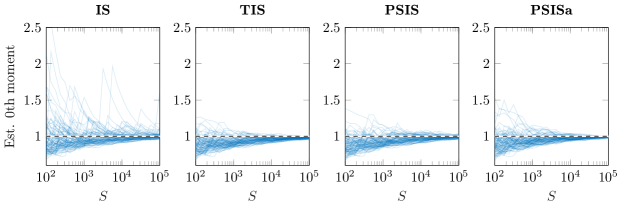
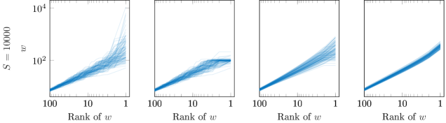
Figure 13: Each graph has 100 blue lines, and each line is the trajectory of the estimated normalization term using different initial random seeds. The first line shows the bias and variance of the different estimators when estimating the zeroth moment (normalization term) as the MCMC sample size increases. The second line shows the distribution of the importance sampling weights when $S=10\,000$. The target and proposal distributions are exponential distributions with mean parameters 1 and 1/3 respectively, and the distribution of ratios has infinite variance.

Figure 13 shows 100 simulations of estimating the normalization term (zeroth moment) using a proposal distribution with mean parameter $1/3$, leading to $k\approx 0.66$ which illustrates the typical behavior of IS, TIS and PSIS when $k\in(0.5,0.7)$. IS has high variability (empirical variance is finite due to the finite number of repeated simulations), while TIS and PSIS produce more stable estimates. For the same 100 simulations, Figure 13 shows the 100 largest IS raw ratios and modified weights from TIS, PSIS, and PSISa. PSISa uses all the raw ratios, that is $M=S$, to fit the generalized Pareto distribution and estimate $\hat{k}$. IS has high variability, TIS truncates the largest weights downwards, while PSIS reduces the variability without biasing the largest weights. PSISa uses more draws to estimate $\hat{k}$ and has smaller variability than PSIS.

Figure 14 shows the bias and standard deviation of the zeroth, first, and second moment estimates with respect to the number of draws $S$ computed from 1000 simulations. This illustrates the typical differences between the methods. IS has the smallest bias but the largest deviation. PSISa has the smallest deviation, and similar bias as PSIS. TIS has the largest bias and with large $S$ similar deviation as PSISa. PSIS has similar bias as PSISa, but slightly larger deviation than PSISa.

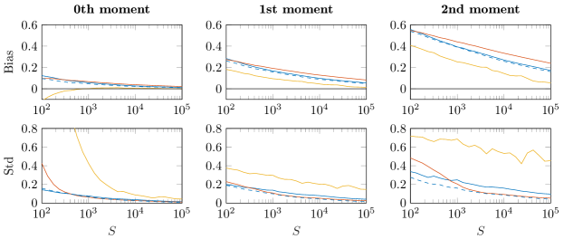
Figure 14: IS is yellow —, TIS is red —, PSIS is blue — and PSISa is blue dashed - -. Bias and standard deviation of the zeroth, first, and second moment estimates with respect to the number of draws $S$ computed from 1000 simulations. Target and proposal distributions are exponential distributions with mean parameters 1 and 1/3 respectively, leading to $k\approx 0.66$.

Figure 2 (in Section 3.2.3) shows the average (over $10\,000$ simulations runs) sample size required for RMSE to be equal to $0.05$, when $\lambda$ is varied from $1.111$ to $20$, which correspond a range of $k$ from $0.1$ to $0.95$. The empirical result fits the theory in Section 3.1 and Appendix A.

Figures 15, 16, and 17 show the RMSE and mean of the MCSE estimates for zeroth, first and second moment estimates with varying $\lambda\in(1.3,1.5,2,3,4,10)$. The $h$-specific $\hat{k}_{h}$ and MCSE work well for first and second moment estimates. Simulations suggest that good results would be obtained with $h(\theta)$ corresponding to higher moments, too. All methods have impractical convergence rates in the case of larger $\hat{k}$ or $\hat{k}_{h}$. With smaller $k$ or $\hat{k}_{h}$ values the errors are similar, but already near $k=0.5$, IS has larger RMSE. IS has finite empirical variance and RMSE with finite repeated simulations, but the tail shape of the error distribution matches the tail shape of the distributions of $r(\theta)$ and $r(\theta)h(\theta)$ revealing the infinite variance in the limit of increasing number of repeated simulations. TIS has larger RMSE than PSIS and PSISa for large $\hat{k}$ values. There is not much difference in RMSE between PSIS and PSISa, demonstrating the diminishing benefit of using a larger sample to estimate $\hat{k}$. The empirical IS MCSE matches the empirical IS RMSE, but has high variance for larger $\hat{k}$ (not shown here). The TIS MCSE estimates have negligible bias when $k<0.5$, but the error is underestimated for $k>0.5$ due to truncation bias dominating the error as discussed in Appendix A. The Monte Carlo estimates for PSIS and PSISa are useful for $k\lesssim 0.7$, with PSISa yielding slightly more accurate error estimates. The results from PSISa show that using larger $M$ (in PSISa $M=S$) would give better estimates, but this works only if those $M$ largest weights are well approximated by the generalized Pareto distribution.

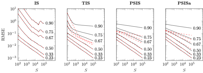
Figure 15: RMSE (black) and the mean of the MCSE estimates (red) for the zeroth moment estimate. Target and proposal distributions are exponential with mean parameters 1 and $1/\lambda$ respectively, with $\lambda\in(1.3,1.5,2,3,4,10)$. The numbers at the end of black lines are average $\hat{k}$ values estimated when $S=10^{5}$.

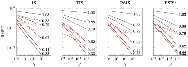
Figure 16: RMSE (black) and the mean of the MCSE estimates (red) for the first moment estimate. Target and proposal distributions are exponential with mean parameters 1 and $1/\lambda$ respectively, with $\lambda\in(1.3,1.5,2,3,4,10)$. For each graph, the lines are ordered with low values of theta at bottom and high values at top, with high $\lambda$ values leading to high RMSE and high $\hat{k}_{h}$. The numbers at the end of black lines are average $h$ specific $\hat{k}_{h}$ values estimated when $S=10^{5}$.

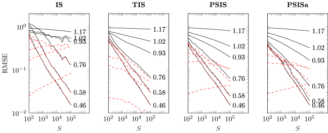
Figure 17: RMSE (black) and the mean of the MCSE estimates (red) for the second moment estimate. Target and proposal distributions are exponential with mean parameters 1 and $1/\lambda$ respectively, with $\lambda\in(1.3,1.5,2,3,4,10)$. For each graph, the lines are ordered with low values of theta at bottom and high values at top, with high $\lambda$ values leading to high RMSE and high $\hat{k}_{h}$. The numbers at the end of black lines are average $h$ specific $\hat{k}_{h}$ values estimated when $S=10^{5}$.

For easier comparison of RMSEs between IS, TIS and PSIS, Figure 1 shows the relative RMSEs.

Figure 18 shows how the relative convergence rate depends on $h$-specific $\hat{k}_{h}$ estimates and matches the theoretical results in Appendix A. For PSIS we observe convergence rates as discussed in Section 3.2.3 and Appendix A. The shown $\hat{k}_{h}$ are estimated using the mean from 1000 simulations, with $S=10^{5}$ for each simulation. Empirical convergence rates are estimated by a linear fit to the RMSE results illustrated in Figures 15–17. Previously in the literature, the focus has been mostly on the binary decision between $k<0.5$ and $k\geq 0.5$. As discussed in Section 3.2.6 and Appendix B, with finite sample size the PSIS convergence rate starts to differ from CLT convergence rate approximately when $k>0.5-0.5/\log_{10}(S)$. In this and the other experiments in the paper, the convergence rate at $k=0.5$ is close to matches well the theoretically predicted $1-1/\log(S)$, for example $0.89$ when $S=2000$. Correspondingly at $k=0.7$, the convergence rate is close to $\alpha\approx 0.6$ which matches the theoretical $2-2k$. In this experiment we added results for $\lambda\in(1.9,2.1)$ which have $k$ just below and above $0.5$, illustrating that there is no sharp transition. A dashed line has been drawn from $k=0.5,\alpha=1$ to $k=0,\alpha=0$ to illustrate the asymptotic behavior when $S\rightarrow\infty$. Based on analytic consideration, we assume that $h$ specific $\hat{k}_{h}$ (as described in Section 2.2) for $\theta r(\theta)$ and $\theta^{2}r(\theta)$ (first and second moment) are not as accurate as $\hat{k}$ estimates for $r(\theta)$ (zeroth moment). This is likely explanation why the corresponding empirical convergence rate curves go slightly beyond the theoretical line. PSISa has better relative convergence rate due to additional variance reduction by using $M=S$, but the difference is small and using $M=S$ is not usually applicable as the whole distribution is not Pareto distribution.

Figure 18: Practical convergence rates for PSIS and PSISa estimating zeroth (blue), first (red), and second (yellow) moments. Target and proposal distributions are exponential with mean parameters 1 and $1/\lambda$ respectively, with $\lambda\in(1.3,1.5,1.9,2,2.1,3,4,10)$. The circles in each line correspond to the results with different $\lambda$, with higher $\lambda$ values leading to lower convergence rates and higher $\hat{k}$ values. The $\hat{k}$ estimates in case of first and second moments depend on $h$. Dotted horizontal lines at $0.87$ and $0.6$ show the typical convergence rates at $\hat{k}=0.5$ and $\hat{k}=0.7$ for several different experiments in this paper.

D.2 Univariate normal and Student’s $t$

The previous example with exponential target and proposal is especially suited for PSIS, as the whole importance ratio distribution is well fitted with the generalized Pareto distribution. In this section, we consider various univariate target and proposal distribution combinations to show the behavior in the case of different target-proposal tail combinations. In the next section we examine the corresponding multivariate cases.

We do not use the simulated example by Ionides, (2008) having the target $p(\theta)=\mbox{normal}(\theta\,|\,0,1)$ and the proposal $g(\theta)=\mbox{normal}(\theta\,|\,0,\sigma)$, as both distributions have the same mean and thus when estimating the first moment the lowest RMSE would be obtained by using identity weights and $\sigma\rightarrow 0$.

To test the performance for the zeroth, first and second moments, we choose the proposal distributions to have different mean and scale than the target distribution. The tested pairs are

1. $p(\theta)=\mbox{normal}(0,1)$, $g(\theta)=\mbox{normal}(\mu,0.8)$: This is a special case with the matching tail shape of the target and proposal leading to a case which is favorable for PSIS.

2. $p(\theta)=t_{20}(0,1)$, $g(\theta)=\mbox{normal}(\mu,0.9)$: This resembles an applied case of using a Gaussian posterior approximation when the target has a thicker tail.

3. $p(\theta)=t_{20}(0,1)$, $g(\theta)=t_{21}(\mu,0.8)$: This resembles an applied case of leave-one-out importance sampling where the proposal has a slightly thinner tail.

4. $p(\theta)=t_{7}(0,1)$, $g(\theta)=t_{8}(\mu,0.8)$: This resembles an applied case of leave-one-out importance sampling where the proposal has a slightly thinner tail, but both having thicker tails than in case 3.

Here we have left out easy univariate examples where the proposal would have a thicker tail than the target. To vary how well the proposal matches the target, the mean of the proposal $\mu$ is varied.

Figure 19 shows plain importance sampling weights for different $\theta$, different target-proposal pairs (1, 3 and 4 in the above list with $\mu=1.5$), and different sample sizes $S$. With increasing sample size $S$ we get more draws from the tails and the differences between the weight functions become more apparent. To better illustrate how the tail shape of the empirical weight distributions change when the sample size $S$ increases, Figure 20 shows the same weights sorted and plotted by rank.

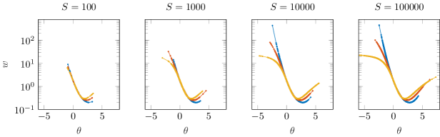
Figure 19: Plain IS weights plotted by $\theta$ for different univariate target-proposal pairs: $p(\theta)=\mbox{normal}(0,1)$, $g(\theta)=\mbox{normal}(1.5,0.8)$ (blue), $p(\theta)=t_{20}(0,1)$, $g(\theta)=t_{21}(1.5,0.8)$ (red), $p(\theta)=t_{7}(0,1)$, $g(\theta)=t_{8}(1.5,0.8)$ (yellow), and different sample sizes $S$.

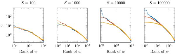
Figure 20: Sorted plain IS weights plotted by rank for different univariate target-proposal pairs: $p(\theta)=\mbox{normal}(0,1)$, $g(\theta)=\mbox{normal}(1.5,0.8)$ (blue), $p(\theta)=t_{20}(0,1)$, $g(\theta)=t_{21}(1.5,0.8)$ (red), $p(\theta)=t_{7}(0,1)$, $g(\theta)=t_{8}(1.5,0.8)$ (yellow), and different sample sizes $S$.

With $S=100$ the weight distributions look similar and the corresponding $\hat{k}$’s are $0.66$, $0.66$, and $0.64$. In the last case the weight distribution is bounded, but $S=100$ is not sufficient to observe the bound with non-negligible probability. As $S$ increases the distributions of the weights eventually look different and the corresponding $\hat{k}$’s are $0.66$, $0.47$, and $-0.28$. In the bounded ratio distribution case, we are observing the bound. This shows that using only a small portion of the raw weights in the tail allows the $\hat{k}$ diagnostic to adapt to the empirically observed tail shape, but also that any finite sample result can be different from a result with much bigger sample size. Figure 20 also illustrates the motivation to truncate the weights at the maximum raw weight value $\max(r_{s})$. This will allow the use of larger $M$ for the Pareto fit to reduce the variance, while being able to adapt when the magnitude of the weights is saturating with increasing $S$.

Based on the above $\hat{k}$ values we may assume that PSIS is beneficial for small $S$, and for cases 3 and 4 when $S$ grows eventually plain IS will also work well. Figure 21 shows the mean RMSE from 1000 simulations for the four different target-proposal pairs as listed above with hand-picked $\mu$ values to illustrate the typical behavior of IS, TIS and PSIS when $\hat{k}\in(0.5,0.7)$ (for very low $\hat{k}$ the differences are negligible and for very high values all methods fail). PSIS is able to adapt well in all cases and has the smallest RMSE in almost all cases. When the proposal distribution has a thin tail (e.g., Gaussian in cases 1 and 2), IS has high variance and the variance remains high with increasing $S$. If the tail of the proposal is thick (e.g. Student’s $t$) and asymptotically the weight distribution has a short tail (small $k$), PSIS performs better than IS for small $S$. Eventually, the RMSE of IS can get as small as the RMSE of PSIS. Most of the time, TIS has a larger RMSE than PSIS. For thick tailed proposals, TIS is not able to adapt well to the changing shape of the empirical weight distribution.

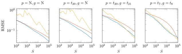
Figure 21: IS is yellow, TIS is red, and PSIS is blue. The mean RMSE from 1000 simulations for the different univariate target-proposal pairs with $\mu$ from left to right being $1.5$, $2$, $2.25$, and $3$.

Figure 22 shows as a representative example of the RMSE and MCSE estimates for zeroth moment estimated with IS, TIS and PSIS in case of $p(\theta)=t_{20}(0,1)$, $g(\theta)=N(\mu,0.9)$. PSIS is more stable, has smaller RMSE than IS, and has more accurate MCSE estimates than TIS.

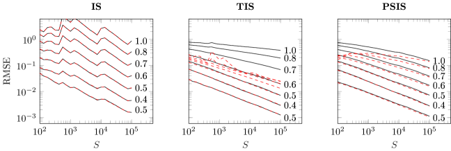
Figure 22: RMSE (black lines) and the mean of the MCSE estimates (red lines) for the zeroth moment estimate. The target distribution is univariate $t_{20}(0,1)$ and the proposal distribution is univariate $\mbox{normal}(\mu,0.9)$, with $\mu\in(0,0.5,1.0,1.5,2.0,2.5,3.0)$. For each graph, the lines are ordered with low values of theta at bottom and high values at top, with high $\theta$ values leading to high RMSE and high $\hat{k}$. The numbers at the end of black lines are average $\hat{k}$ values estimated when $S=10^{5}$.

Figure 23 shows the relative convergence rate with respect to $h$-specific $\hat{k}_{h}$ estimates. We observe similar behavior as in the exponential distribution example, even now the ratio distributions are not exactly Pareto shaped. For thick tail proposal distributions we tend to overestimate $\hat{k}_{h}$ values more than for the thin tailed proposal distributions, but the convergence rates stay good. Given estimated $\hat{k}_{h}$ values, we can use the theoretical result to provide a conservative convergence rate estimate (it’s better the diagnostic is conservative than too optimistic).

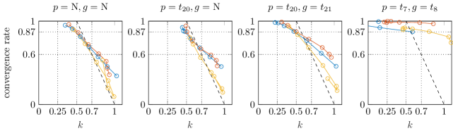
Figure 23: Practical convergence rates for PSIS estimating zeroth (blue –), first (red –) and second (yellow –) moments. Different univariate target-proposal distribution pairs are used in different subplots. $\hat{k}$ estimates in case of first and second moments are $h$ specific. Dotted horizontal lines at $0.87$ and $0.6$ show the typical convergence rates at $\hat{k}=0.5$ and $\hat{k}=0.7$ for several different experiments in this paper.

D.3 Multivariate normal and Student’s $t$

In this section, we consider the isotropic multivariate versions of the four target-proposal pairs as the number of dimensions increases. In addition, we also examine a case where the proposal has thicker tails than the target, and show that with an increasing number of dimensions this will also lead to increasing variability of the weights. The compared target-proposal pairs are

1. $p(\theta)=\mbox{MVN}(\mathbf{0},I)$, $g(\theta)=\mbox{MVN}(0.4\cdot\mathbf{1},0.8I)$

2. $p(\theta)=t_{20}(\mathbf{0},I)$, $g(\theta)=\mbox{MVN}(0.4\cdot\mathbf{1},0.9I)$

3. $p(\theta)=t_{20}(\mathbf{0},I)$, $g(\theta)=t_{21}(0.4\cdot\mathbf{1},0.8I)$

4. $p(\theta)=t_{7}(\mathbf{0},I)$, $g(\theta)=t_{8}(0.4\cdot\mathbf{1},0.8I)$

5. $p(\theta)=\mbox{MVN}(\mathbf{0},I)$, $g(\theta)=t_{7}(0.4\cdot\mathbf{1},0.8I)$

In all these cases, the proposal distribution is just slightly displaced and with slightly narrower scale. The fifth proposal distribution has thicker tails than the target distribution, so that the importance ratios are bounded although that bound can be too far to be observed with a finite sample size. The number of dimensions is varied as $D\in(1,2,4,8,16,32,64)$.

Figure 24 shows the mean RMSE from 1000 simulations for the five different target-proposal pairs as listed above with $D=16$ for all except the last case with $D=32$. The plots illustrate the typical behavior of IS, TIS and PSIS when $0.5<\hat{k}<0.7$. PSIS has the smallest RMSE in all cases. TIS has a slower convergence rate than PSIS. IS is overall more unstable and has higher RMSE. Comparing the case with a thick tailed proposal distribution to the corresponding univariate case, we see that IS requires larger $S$ before beginning to stabilize. The rightmost subplot illustrates that even if the proposal distribution has thicker tails than the target distribution and the importance ratios are bounded, the variance of the importance ratio distribution can be high when the number of dimensions $D$, and IS is not a safe choice in finite sample case.

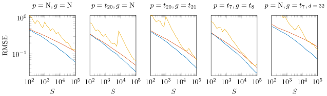
Figure 24: IS is yellow —, TIS is red —, and PSIS is blue —. The mean RMSE from 1000 simulations for the different multivariate target-proposal pairs with $D=16$ for all except the last one with $D=32$ (the number of dimensions for each plot were chosen to show interesting behavior between too easy and too difficult).

Figure 25 shows a representative example of the RMSE and Monte Carlo estimates for zeroth moment estimated with IS, TIS and PSIS with $p(\theta)=t_{20}(\mathbf{0},I)$, $g(\theta)=N(0.4\cdot\mathbf{1},0.9I)$. PSIS is more stable, has smaller RMSE than IS and TIS, and has more accurate MCSE estimates than TIS. All methods eventually fail as the number of dimensions increases and even a small difference in the distributions is amplified. Having a bounded importance ratios and finite variance, does not prevent the behavior to be indistinguishable from the infinite variance case in finite sample case. In these multivariate examples, we observe sudden large jumps also for TIS. Truncation in TIS fails when there is one extremely large weight that causes the truncation level to rise so high that other large weights are not truncated. PSIS performs better in the same situation, as one extreme large weight doesn’t affect the generalized Pareto fit as much.

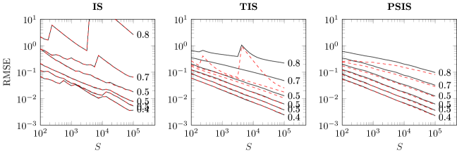
Figure 25: RMSE (black line) and the mean of the MCSE estimates (red dashed line) for the zeroth moment estimate. The target distribution is multivariate $t_{20}(\mathbf{0},I)$ and the proposal distribution is multivariate $\mbox{MVN}(0.4\mathbf{1},0.9I)$, with the number of dimensions $D\in(1,2,4,8,16,32,64)$. For each graph, the lines are ordered with low values of $D$ at bottom and high values at top, with high $D$ values leading to high RMSE and high $\hat{k}$. The numbers at the end of black lines are average $\hat{k}$ values estimated when $S=10^{5}$.

Figure 26 shows the practical convergence rate with respect to the $h$-specific $\hat{k}$ estimates. We observe similar behavior as in the univariate example. As we saw before, the observed convergence rate with respect to $\hat{k}$ is close to the theoretical result.

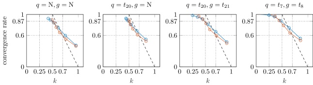
Figure 26: Practical convergence rates for PSIS estimating zeroth (blue, and first (red) moments. Different multivariate target-proposal distribution pairs are used in different subplots. $\hat{k}$ estimates in case of first and second moments are $h$ specific. Dotted horizontal lines at $0.87$ and $0.6$ show the typical convergence rates at $\hat{k}=0.5$ and $\hat{k}=0.7$ for several different experiments in this paper.

Appendix E $h$-specific $\hat{k}_{h}$

In Section 3 we defined $h$-specific $\hat{k}_{h}$ as maximum of $\hat{k}$ estimated with $M$ smallest and $M$ largest values of $h(\theta)r(\theta)$ (left and right tail). As we choose the larger value from two estimated values with uncertainty, $\hat{k}_{h}$ has positive bias when those values are close to each other. We think this bias is acceptable as a conservative choice. The benefits of this approach are that it is simple and it is also natural when assessing tail shape of $h(\theta)$ given Monte Carlo draws (i.e., $r(\theta)=1$).

In an earlier version of this paper we proposed to estimate $h$-specific $\hat{k}_{h}$ for $\sqrt{1+h(\theta)^{2}}\,r(\theta)$, a form used by Epifani et al., (2008) to avoid zero values when proving conditions for CLT for different IS-LOO influence measures. This form is also close to $|h(\theta)|r(\theta)$, which has been commonly used to evaluate $h$-specific variance of IS estimators (see, e.g. Owen,, 2013, Ch. 9). The benefit is that we could estimate just one $\hat{k}_{h}$, but the downside is that the tail can then be a mixture of two tails, and in a finite sample case this can lead to underestimating $k_{h}$. In our experiments the two tail diagnostic of $h(\theta)r(\theta)$ worked slightly better over different scenarios.

Although we recommend use of $h$-specific $\hat{k}_{h}$, we do not recommend smoothing $h(\theta)r(\theta)$. Smoothing $r(\theta)$ and $h(\theta)r(\theta)$ separately introduces an additional bias in the normalization, which based on our experiments leads in some cases to noticeable increase in the estimation error.

Appendix F Marginal distribution of $k$

The method by Zhang and Stephens, (2009) uses profile likelihood, weakly informative empirical data based prior, and quadrature integration. Zhang and Stephens, (2009) analyse the derived posterior mean estimate $\hat{k}$, for which they report only a small bias. In this paper we focused on using $\hat{k}$ as the diagnostic, as we didn’t find additional benefit from estimating, for example, the probability that $k<0.5$ or that $k<0.7$. However, knowing the associated uncertainty can be sometimes useful to assess what could be learned by increasing the sample size in importance sampling.

Zhang and Stephens, (2009) use parameterization $(\theta,k)$, where $\theta=\sigma/k$. Figure 27a shows the joint likelihood, joint posterior, and the profile curve and the quadrature points. The profile likelihood for $\theta$ is the likelihood along a curve with $k$ chosen to maximize the likelihood. When the prior is set only on $\theta$, the profile posterior is determined along the same curve. Zhang and Stephens, (2009) select the location of the quadrature points along the profile curve and spacing is determined by the prior. Then the quadrature weights to determine the profile posterior mean are simply the normalized likelihood values at the quadrature points. After finding the posterior mean $\hat{\theta}$, the estimate $\hat{k}$ comes from the profile curve, and $\hat{\sigma}=\hat{\theta}/\hat{k}$.

Zhang and Stephens, (2009) discuss only point estimates $\hat{k}$ and $\hat{\sigma}$, but we demonstrate that the profile posterior can be used as an approximation for the marginal posterior of $k$. When computing the posterior mean with quadrature, the quadrature weights are proportional to the likelihood as the quadrature points are spaced according to the prior density. To plot the profile posterior, we compute the normalized posterior densities at the quadrature points. Figure 27b compares the profile posterior and true marginal posterior (computed from the exact two dimensional posterior using adaptive quadrature integration). Figure 27b also illustrates the uncertainty with different values of $M=(20,100,1000)$, which correspond to tail sample sizes using the proposed rule for total sample sizes $S=(100,1111,111\,111)$.

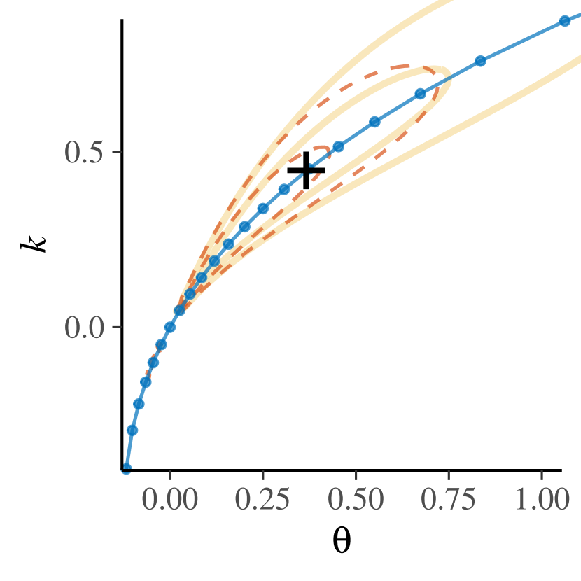
(a)

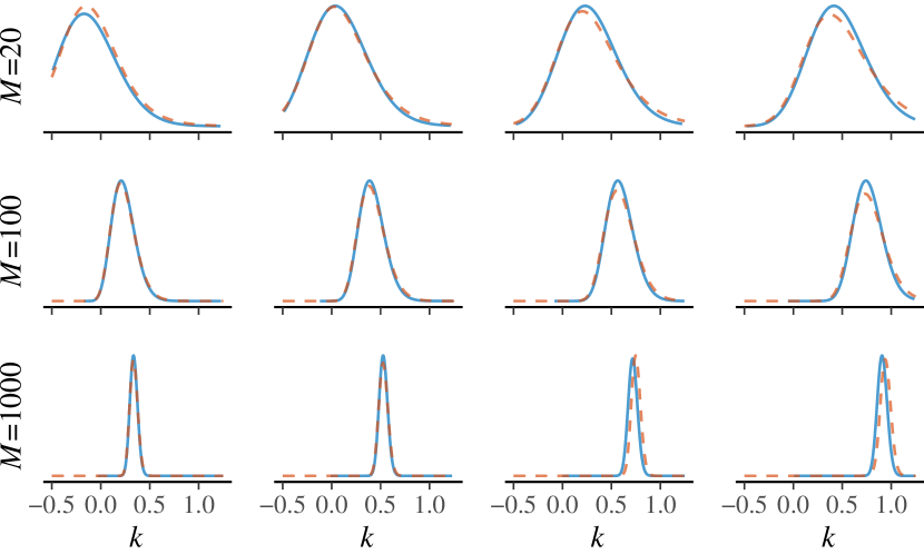
(b)

Figure 27: (a) The joint likelihood, the joint posterior, the profile curve and the quadrature points, and the profile posterior mean $(\hat{\theta},\hat{k})$ marked with $\boldsymbol{+}$, based on 20 observations simulated from the generalized Pareto distribution (GPD) with $k=0.7$ and $\sigma=1$. (b) Posterior marginal of $k$ estimated from the profile posterior, and exact posterior marginal (dashed line). Rows show example marginals for simulated data with sizes of 20, 100, and 1000. Columns show example marginals for simulated data generated from GPD with $k\in(0.3,0.5,0.7,0.9)$. The third subplot on the top row is for the same data as in the plot (a).

Zhang, (2010) presented an alternative empirical prior which in case of small sample sizes produces estimates with smaller bias for estimating $\sigma$ and $k$ when $k>0.5$, but has slightly lower efficiency for estimating $k$ when $0<k<4$. Compared to the uncertainty in $k$ (see Figure 27b), the small differences in bias and efficiency (as reported by Zhang,, 2010) when $k\in(0,1)$ do not make a practical difference in PSIS or diagnostics.

Appendix G Regularization of Pareto fit for small $S$

To reduce the variance of the $\hat{k}$ estimate for small $S$ ($S$ less than about 1000), we use an additional regularization,

$$\hat{k}=(M\hat{k}+10\cdot 0.5)/(M+10),$$

which corresponds approximately to a weakly informative Gaussian prior that has a weight of 10 observations from the tail shrinking toward $0.5$. If $S=100$ and using the proposed rule to choose $M=20$, we see that $\hat{k}$ is strongly regularized. If $S=1000$ and using the proposed rule to choose $M=95$, we see that the regularization has only weight of one tenth of the data. This regularization adds bias toward $0.5$, but based on our simulation results, this reduced the variance and RMSE of the PSIS estimates with small $S$, without introducing significant bias or affecting the RMSE for larger $S$. In many applications we would assume $S>1000$, but in sequential and iterative methods such as particle filters and black box variational inference we may want to use small $S$ for computational speed issues.

Appendix H Adjusting $M$ in case of dependent MCMC draws

We adjust the algorithm in the following way to take into account the usually smaller effective sample size of dependent MCMC draws. Due to correlated MCMC draws, we use more ratios in the tail to keep the variance of $\hat{k}$ in control. We adjust the number of tail ratios used as $M=3\sqrt{S/R_{\mathrm{eff,MCMC}}}$ if $S>225$ or $M=S/5$ for lower values of $S$, where $R_{\mathrm{eff,MCMC}}=S_{\mathrm{eff,MCMC}}/S$ is the estimated relative efficiency of the MCMC draws, and the effective sample size $S_{\mathrm{eff,MCMC}}$ for $r(\theta)$ is computed using the split-chain effective sample size estimate method (Vehtari et al.,, 2021). This effective sample size is not directly the effective sample size for $\hat{k}$, but it is related and much easier to compute.

Appendix I Stan program for Gaussian linear regression on the stack loss data

data {  int<lower=0> N;  int<lower=0> p;  vector[N] y;  matrix[N,p] x;}// to standardize the x’stransformed data {  matrix[N,p] z;  vector[p] mean_x;  vector[p] sd_x;  real sd_y <- sd(y);  for (j in 1:p) {    mean_x[j] = mean(col(x,j));    sd_x[j] = sd(col(x,j));    for (i in 1:N)      z[i,j] = (x[i,j] - mean_x[j]) / sd_x[j];  }}parameters {  real beta0;  vector[p] beta;  real<lower=0> sigmasq;  real<lower=0> phi;}transformed parameters {  real<lower=0> sigma;  vector[N] mu;  sigma = sqrt(sigmasq);  mu = beta0 + z * beta;}model {  beta0 ~ normal(0, 100);  phi ~ cauchy(0, sd_y);  beta ~ normal(0, phi);  sigmasq ~ inv_gamma(0.1, 0.1);  y ~ normal(mu, sigma);}generated quantities {  vector[N] log_lik;  for (i in 1:N)    log_lik[i] = normal_lpdf(y[i] | mu[i], sigma);}

References

- Agapiou et al., (2017) Agapiou, S., Papaspiliopoulos, O., Sanz-Alonso, D., and Stuart, A. (2017). Importance sampling: Intrinsic dimension and computational cost. Statistical Science, 32(3):405–431.
- Aittomäki, (2016) Aittomäki, V. (2016). MicroRNA regulation in breast cancer—a Bayesian analysis of expression data. Master’s thesis, Aalto University.
- Aure et al., (2015) Aure, M. R., Jernström, S., Krohn, M., Vollan, H. K., Due, E. U., Rødland, E., Kåresen, R., Ram, P., Lu, Y., Mills, G. B., Sahlberg, K. K., Børresen-Dale, A. L., Lingjærde, O. C., and Kristensen, V. N. (2015). Integrated analysis reveals microRNA networks coordinately expressed with key proteins in breast cancer. Genome Medicine, 7(1):21.
- Balkema and de Haan, (1974) Balkema, A. A. and de Haan, L. (1974). Residual life time at great age. The Annals of Probability, 2(5):792 – 804.
- Bickel, (1967) Bickel, P. J. (1967). Some contributions to the theory of order statistics. In Berkeley Symposium on Mathematical Statistics and Probability, pages 575–591.
- Bingham et al., (2019) Bingham, E., Chen, J. P., Jankowiak, M., Obermeyer, F., Pradhan, N., Karaletsos, T., Singh, R., Szerlip, P., Horsfall, P., and Goodman, N. D. (2019). Pyro: Deep universal probabilistic programming. Journal of Machine Learning Research, 20(1):973–978.
- Blom, (1958) Blom, G. (1958). Statistical Estimates and Transformed Beta-Variables. Wiley.
- Bouchaud and Georges, (1990) Bouchaud, J.-P. and Georges, A. (1990). Anomalous diffusion in disordered media: statistical mechanisms, models and physical applications. Physics reports, 195(4-5):127–293.
- Bugallo et al., (2017) Bugallo, M. F., Elvira, V., Martino, L., Luengo, D., Miguez, J., and Djuric, P. M. (2017). Adaptive importance sampling: The past, the present, and the future. IEEE Signal Processing Magazine, 34(4):60–79.
- (10) Bürkner, P.-C., Gabry, J., and Vehtari, A. (2020a). Approximate leave-future-out cross-validation for Bayesian time series models. Journal of Statistical Computation and Simulation, 90:2499–2523.
- (11) Bürkner, P.-C., Gabry, J., and Vehtari, A. (2020b). Efficient leave-one-out cross-validation for Bayesian non-factorized normal and Student- models. Computational Statistics, 36:1243–1261.
- Cappé et al., (2004) Cappé, O., Guillin, A., Marin, J.-M., and Robert, C. P. (2004). Population Monte Carlo. Journal of Computational and Graphical Statistics, 13(4):907–929.