Fast Rates in Statistical and Online Learning

Abstract

The speed with which a learning algorithm converges as it is presented with more data is a central problem in machine learning — a fast rate of convergence means less data is needed for the same level of performance. The pursuit of fast rates in online and statistical learning has led to the discovery of many conditions in learning theory under which fast learning is possible. We show that most of these conditions are special cases of a single, unifying condition, that comes in two forms: the central condition for ‘proper’ learning algorithms that always output a hypothesis in the given model, and stochastic mixability for online algorithms that may make predictions outside of the model. We show that under surprisingly weak assumptions both conditions are, in a certain sense, equivalent. The central condition has a re-interpretation in terms of convexity of a set of pseudoprobabilities, linking it to density estimation under misspecification. For bounded losses, we show how the central condition enables a direct proof of fast rates and we prove its equivalence to the Bernstein condition, itself a generalization of the Tsybakov margin condition, both of which have played a central role in obtaining fast rates in statistical learning. Yet, while the Bernstein condition is two-sided, the central condition is one-sided, making it more suitable to deal with unbounded losses. In its stochastic mixability form, our condition generalizes both a stochastic exp-concavity condition identified by Juditsky, Rigollet and Tsybakov and Vovk’s notion of mixability. Our unifying conditions thus provide a substantial step towards a characterization of fast rates in statistical learning, similar to how classical mixability characterizes constant regret in the sequential prediction with expert advice setting.

Keywords: statistical learning theory, fast rates, Tsybakov margin condition, mixability, exp-concavity

1 Introduction

Alexey Chervonenkis jointly achieved several significant milestones in the theory of machine learning: the characterization of uniform convergence of relative frequencies of events to their probabilities (Vapnik and Chervonenkis, 1971), the uniform convergence of means to their expectations (Vapnik and Chervonenkis, 1981), and the ‘key theorem in learning theory’ showing the relationship between the consistency of empirical risk minimization (ERM) and the uniform one-sided convergence of means to expectations (Vapnik and Chervonenkis, 1991); (Vapnik, 1998, Chapter 3). Two outstanding features of these contributions are that they characterized the phenomenon in question, and the quantitative results are parametrization independent in the sense that they do not depend upon how elements of the hypothesis class $\mathcal{F}$ are parameterized, only on global (effectively geometric) properties of $\mathcal{F}$. With his co-author Vladimir Vapnik, Alexey Chervonenkis also presented quantitative bounds on the deviation between the empirical and expected risk as a function of the sample size $n$. These are used for the theoretical analysis of the statistical convergence of ERM algorithms, which are central to machine learning. According to Vapnik (1998, p. 695), in his 1974 book co-authored by Chervonenkis (Vapnik and Chervonenkis, 1974) they presented ‘slow’ and ‘fast’ bounds for ERM when used with 0-1 loss. They showed that in the realizable or ‘optimistic’ case (where there is an $f\in\mathcal{F}$ that almost surely predicts correctly, so that the minimum achievable risk is zero) one can achieve fast $O(1/n)$ convergence as opposed to the ‘pessimistic’ case where one does not have such an $f$ in the hypothesis class and the best uniform bound is $O(1/\sqrt{n})$ (Vapnik, 1998, page 127). This difference is important because if one is in such a ‘fast rate’ regime, one can achieve good performance with less data.

The present paper makes several further contributions along this path first delineated by Vapnik and Chervonenkis. We focus upon the distinction between slow and fast learning. As shown in the special case of squared loss by Lee et al. (1998) and log loss by Li (1999), if the hypothesis class is convex, one can still attain fast $O(1/n)$ convergence even in the agnostic (pessimistic) setting. Such convergence results, like those of Vapnik and Chervonenkis, are uniform — they hold for all possible target distributions. When the hypothesis class is not convex, one cannot attain a uniform fast bound for ERM (Mendelson, 2008a), and it is not known whether fast rates are possible for any algorithm at all; however, one can obtain a non-uniform bound (Mendelson and Williamson, 2002; Mendelson, 2008b). Such bounds are necessarily dependent upon the relationships between the components $(\ell,\mathcal{P},\mathcal{F})$ of a statistical decision problem or learning task. Here $\ell$ is the loss, $\mathcal{F}$ the hypothesis class, and $\mathcal{P}$ the (possibly singleton) class of distributions which, by assumption, contains the unknown data-generating distribution. Often one can assume large classes of $\mathcal{P}$ and still obtain bounds that are relatively uniform, i.e. uniform over all $P\in\mathcal{P}$. We identify a central condition on decision problems $(\ell,\mathcal{P},\mathcal{F})$ — where $\ell$ may be unbounded — that, in its strongest form, allows $O(1/n)$ rates for so-called ‘proper’ learning algorithms that always output a member of $\mathcal{F}$. In weaker forms, it allows rates in between $O(1/\sqrt{n})$ and $O(1/n)$.

As a second contribution, we connect the above line of work (within the traditional stochastic setting) to a parallel development in the worst-case online sequence prediction setting. There, one makes no probabilistic assumptions at all, and one measures convergence of the regret, that is, the difference between the cumulative loss attained by a given algorithm on a particular sequence with the best possible loss attainable on that sequence (Cesa-Bianchi and Lugosi, 2006). This work, due in large part to Vovk (1990, 1998, 2001), shares one aspect of Vapnik and Chervonenkis’ approach — it achieves a characterization of when fast learning is possible in the online individual sequence-setting. Since there is no $\mathcal{P}$ in this setting, the characterization depends only upon the loss $\ell$, and in particular whether the loss is mixable. As shown in Section 4, our second key condition, stochastic mixability, is a generalization of Vovk’s earlier notion. Briefly, when $\mathcal{P}$ is the set of all distributions on a domain, stochastic mixability is equivalent to Vovk’s classical mixability. Stochastic mixability of $(\ell,\mathcal{P},\mathcal{F})$ for general $\mathcal{P}$ then indicates that fast rates are possible in a stochastic on-line setting, in the worst-case over all $P\in\mathcal{P}$.

The main contribution in this paper is to show, first, that a range of existing conditions for fast rates (such as the Bernstein condition, itself a generalization of the Tsybakov condition) are either special cases of our central condition, or special cases of stochastic mixability (such as original mixability and (stochastic) exp-concavity); and second, to show that under surprisingly weak conditions the central condition and stochastic mixability are in fact equivalent — thus there emerges essentially a single condition that implies fast rates in a wide variety of situations. Our central and stochastic mixability condition improve in several ways on the existing conditions that they generalize and unify. For example, like the uniform convergence condition in Vapnik and Chervonenkis’ original ‘key theorem of learning theory’ (Vapnik and Chervonenkis, 1991), but unlike the Bernstein fast rate condition, our conditions are one-sided which, as forcefully argued by Mendelson (2014), seems as it should be; Example 5.44 explains and illustrates the difference between the two- and one-sided conditions. Like Vapnik and Chervonenkis’ uniform convergence condition and Vovk’s classical mixability, but unlike the stochastic and individual-sequence exp-concavity conditions, our conditions are parametrization independent (Section 4.2.2). Finally, unlike the assumptions for classical mixability (Vovk, 1998), we do not require compactness of the loss function’s domain. We hasten to add though that for unbounded losses, several important issues are still unresolved — for example, if under some $P\in\mathcal{P}$ and with some $f\in\mathcal{F}$ the distribution of the loss has polynomial tails, then some of our equivalences break down (Section 5.2).

One final historical precursor deserves mention. Statistical convergence bounds rely on bounds on the tails of certain random variables. In Section 7 we show how, for bounded losses, the central condition (4) directly controls the behaviour of the cumulant generating function of the excess loss random variable. The geometric insight behind this result, Figure 3, previously was used, unbeknownst to us when carrying out the work originally (Mehta and Williamson, 2014), by Claude Shannon (1956). It is fitting that our tribute to Alexey Chervonenkis can trace its history to another such giant of the theory of information processing.

1.1 Why Read This Paper? Our Most Important Results

Below, we highlight the core contributions of this work. A more comprehensive overview is in Section 2 and the diagram on page 1, which summarizes all results from the paper.

• We introduce the $v$-stochastic mixability condition on decision problems (Equation (8), Definition 4.17 and 5.46), a strict generalization of Vovk’s classical mixability (Vovk, 1990, 1998, 2001; van Erven et al., 2012a), exp-concavity (Kivinen and Warmuth, 1999; Cesa-Bianchi and Lugosi, 2006) and stochastic exp-concavity, a condition identified implicitly by Juditsky et al. (2008) and used by e.g. Dalalyan and Tsybakov (2012). Here $v:\mathbb{R}^{+}_{0}\rightarrow\mathbb{R}^{+}_{0}$ is a nondecreasing nonnegative function. In the important special case that $v\equiv\eta$ is constant, we say that (strong) stochastic mixability holds. Proposition 4.21 shows that in that case, with finite $\mathcal{F}$, Vovk’s aggregating algorithm for on-line prediction in combination with an online-to-batch conversion achieves a learning rate of $O(1/n)$; if the $v$-condition holds for sublinear $v$ with $v(0)=0$, intermediate rates between $O(1/\sqrt{n})$ and $O(1/n)$ are obtained. These results hold under no further conditions at all, in particular for unbounded losses. Interest: the condition being a strict generalization of earlier ones, it shows that we can get fast rates for some situations for which this was was hitherto unknown.

• We introduce the $v$-central condition (Equations (4), (5), (6), (10), Definition 3.4 and 5.40). As we show in Theorem 5.41, for bounded losses and $v$ of the form $v(x)=Cx^{\alpha}$, it generalizes the Bernstein condition (Bartlett and Mendelson, 2006), itself a generalization of the Tsybakov margin condition (Tsybakov, 2004). If $v\equiv\eta$ is constant, we just say that the (strong) central condition holds. In that case, with (unbounded) log-loss, it generalizes a (typically nameless) condition used to obtain fast rates in Bayesian and minimum description length (MDL) density estimation in misspecification contexts (Li, 1999; Zhang, 2006a, b; Kleijn and van der Vaart, 2006; Grünwald, 2011; Grünwald and van Ommen, 2014). These are all conditions that allow for fast rates for proper learning, in which the learning algorithm always outputs an element of $\mathcal{F}$.

  (i) For convex $\mathcal{F}$, we prove that the strong $\eta$-central condition and the strong $\eta$-stochastic mixability are equivalent, under weak conditions (Theorem 4.33 in conjunction with Proposition 4.27 and Theorem 3.13 in conjunction with Proposition 4.28). Interest: This shows that existing fast rate conditions for $O(1/n)$ rates in online learning are related to fast rate conditions for $O(1/n)$ rates for proper learning algorithms such as ERM — even though such conditions superficially look very different and have very different interpretations: existence of a ‘substitution function’ (mixability) vs. the exponential moment of a loss difference constituting a supermartingale (central condition).

  (ii) We prove (a) that for bounded losses, the strong central condition always implies fast $O(1/n)$ rates for ERM and the $v$-central condition implies intermediate rates (Theorem 7.56). The equivalence between $\eta$-mixability and the central condition and Proposition 4.21 mentioned above imply that, (b), the central condition implies fast rates in many more conditions, even with unbounded losses. We also show (c) that there exist decision problems with unbounded losses in which the central condition holds, the Bernstein condition does not hold, and we do get fast rates. Interest: first, while fast and intermediate rates under the $v$-central condition with bounded loss can also be derived from existing results, our proof is directly in terms of the central condition and yields better constants. Second, results (a)-(c) above lead us to conjecture that there exist some very weak condition (much weaker than bounded loss) such that for sublinear $v$, the $v$-central condition together with this extra condition always implies sublinear rates. Establishing such a result is a major goal for future work.

• Under mild conditions, the $v$-central condition is equivalent to a third condition, the pseudoprobability convexity (PPC) condition — (7) and Definition 3.5 and 5.40. Interest: for the constant $v\equiv\eta$ case ($O(1/n)$ rates), the PPC condition provides a clear geometric and a data-compression interpretation of the $v$-central condition. For bounded losses and general $v$, it implies that a problem must have unique minimizers in a certain sense (Proposition 5.48), giving further insight into the fast rates phenomenon.

• In some cases with nonconvex $\mathcal{F}$, ERM and other proper learning algorithms achieve a suboptimal $O(1/\sqrt{n})$ rate, whereas online methods combined with an online-to-batch convergence get $O(1/n)$ rates in expectation (Audibert, 2007). Now the implication ‘strong stochastic mixability $\Rightarrow$ strong central condition ’ (Theorem 3.13 in conjunction with Proposition 4.28, already mentioned under 2(i)) holds whenever the risk minimizer within $\mathcal{F}$ coincides with the risk minimizer within the convex hull of $\mathcal{F}$. Thus, as long as this is the case, there is no inherent rate advantage in improper learning — if $\eta$-stochastic mixability holds so that (improper) online methods achieve an $O(1/n)$-rate, so will the (proper) ERM method. Theorem 7.56 implies this for bounded losses; we conjecture that the same holds for unbounded losses. Interest: This insight helps understand when improper learning can and cannot be helpful for general losses, something that was hitherto only well-understood for the squared loss on a bounded domain (Lecué, 2011).

Figure 1:

2 Introduction to and Overview of Results

To facilitate reading of this long paper, we provide an introductory summary of all our results. By reading this section alongside the ‘map’ of conditions and their relationships on page 1, the reader should get a good overview of our results. We start below with some notational and conceptual preliminaries, and continue in Section 2.2 with a discussion of the central condition, followed by a section-by-section description of the paper.

2.1 Decision problems and Risk

We consider decision problems which, in their most general form, can be specified as a four-tuple $(\ell,\mathcal{P},\mathcal{F},\mathcal{F}_{\textnormal{d}})$ where $\mathcal{P}$ is a set of distributions on a sample space $\mathcal{Z}$, and the goal is to make decisions that are essentially as good as the best decision in the model $\mathcal{F}$ ($\mathcal{F}$ is often called an ‘hypothesis space’ in machine learning). We will allow the decision maker to make decisions in a decision set $\mathcal{F}_{\textnormal{d}}$ which is usually taken equal to, or a superset of, $\mathcal{F}$ but for mathematical convenience is also allowed to be a subset of $\mathcal{F}$. The quality of decisions will be measured by a loss function $\ell\colon\mathcal{F}_{\ell}\times\mathcal{Z}\rightarrow[-B,\infty]$ for arbitrary $B\geq 0$ where a smaller loss means better predictions, and $\mathcal{F}_{\ell}\supseteq\mathcal{F}\cup\mathcal{F}_{\textnormal{d}}$ is the domain of the loss. As further notation we introduce the component functions $\ell_{f}(z)=\ell(f,z)$ and for any set $\mathcal{G}$ we let $\Delta(\mathcal{G})$ denote the set of distributions on $\mathcal{G}$ (implicitly assuming that $\mathcal{G}$ is a measurable set, equipped with an appropriate $\sigma$-algebra). A loss function $\ell$ is called bounded if for some $B\geq 0$, for all $f\in\mathcal{F}_{\ell}$ and all $P\in\mathcal{P}$, we have $|\ell_{f}(Z)|\leq B$ almost surely when $Z\sim P$. When $\mathcal{F}_{\ell}$ is a set for which this is well-defined, for any $\mathcal{F}\subset\mathcal{F}_{\ell}$ we denote by $\operatorname*{\operatorname{co}}(\mathcal{F})\subseteq\mathcal{F}_{\ell}$ the convex hull of $\mathcal{F}$.

Now fix some decision problem $(\ell,\mathcal{P},\mathcal{F},\mathcal{F}_{\textnormal{d}})$. The risk of a predictor $f\in\mathcal{F}_{\ell}$ with respect to $P\in\mathcal{P}$ is defined, as usual, as

$$R(P,f)=\operatorname*{{\bf E}}_{Z\sim P}[\ell_{f}(Z)],$$ (1)

where $Z$ is a random variable mapping to outcomes in $\mathcal{Z}$ and, in general, $R(P,f)$ may be infinite. However, for the remainder of the paper we will only consider tuples $(\ell,\mathcal{P},\mathcal{F},\mathcal{F}_{\textnormal{d}})$ such that for all $P\in\mathcal{P}$, there exists at least one $f^{\circ}\in\mathcal{F}$ with $R(P,f^{\circ})<\infty$ and hence $P(\ell_{f^{\circ}}(Z)=\infty)=0$. A learning algorithm or estimator is a (computable) function from $\cup_{n\geq 0}\mathcal{Z}^{n}$ to $\mathcal{F}_{\textnormal{d}}$ that, upon observing data $Z_{1},\ldots,Z_{n}$, outputs some $\hat{f}_{n}\in\mathcal{F}_{\textnormal{d}}$. Following standard terminology, we call a learning algorithm proper (Lee et al., 1996; Alekhnovich et al., 2004; Urner and Ben-David, 2014) if its outputs are restricted to the set $\mathcal{F}$, i.e. $\mathcal{F}=\mathcal{F}_{\textnormal{d}}$. Examples of this setting, which has also been called in-model estimation (Grünwald and van Ommen, 2014), include ERM and Bayesian maximum a posteriori (MAP) density estimation. For notational convenience, in such cases we identify a decision problem with the triple $(\ell,\mathcal{P},\mathcal{F})$. We only consider $\mathcal{F}\neq\mathcal{F}_{\textnormal{d}}$ in Section 4 and 6 on on-line learning, where $\mathcal{F}_{\textnormal{d}}$ is often taken to be $\operatorname*{\operatorname{co}}(\mathcal{F})$; for example, $\mathcal{F}$ may be a set of probability densities (Example 2.2) and the algorithm may be Bayesian prediction, which predicts with the Bayes predictive distribution (Section 3.3), a mixture of elements of $\mathcal{F}$ which is hence in $\operatorname*{\operatorname{co}}(\mathcal{F})$. One of our main insights, discussed in Section 4.3.3, is understanding when the weaker conditions that allow fast rates for improper learning transfer to the proper learning setting. In the stochastic setting, the rate (in expectation) of a learning algorithm is the quantity

$$\sup_{P\in\mathcal{P}}\ \ \left\{\ \operatorname*{{\bf E}}_{\mathbf{Z}\sim P}\left[R(P,\hat{f}_{n})\right]-\inf_{f\in\mathcal{F}}R(P,f)\ \right\},$$ (2)

where $\mathbf{Z}=(Z_{1},\ldots,Z_{n})$ are $n$ i.i.d. copies of $Z$. The rate of a learning algorithm can usually be bounded, up to $\log n$ factors, as $(\text{\sc comp}_{n}(\mathcal{F})/n)^{\alpha}$ for some $\alpha$ between $1/2$ and $1$. Here $\text{\sc comp}_{n}(\mathcal{F})$ is some measure of the complexity of $\mathcal{F}$ which may or may not depend on $n$, such as its codelength, its VC-dimension in classification, an upper bound on the KL-divergence between prior and posterior in PAC-Bayesian approaches, or the logarithm of the number of elements of an $\varepsilon$-net, with $\varepsilon$ determined by sample size, and so on. In the simplest case, with $\mathcal{F}$ finite, complexity is invariably bounded independently of $n$ (usually as $\log|\mathcal{F}|$), and whenever for a decision problem $(\ell,\mathcal{P},\mathcal{F},\mathcal{F}_{\textnormal{d}})$ with finite $\mathcal{F}$ there exists a learning algorithm achieving the rate $O(1/n)$, we say that the problem allows for fast rates.

In the remainder of this section we make the following simplifying assumption.

Assumption A

(Minimal Risk Achieved) For all $P\in\mathcal{P}$, the minimal risk $R(P,f)$ over $\mathcal{F}$ is achieved by some $f^{*}\in\mathcal{F}$ depending on $P$, i.e.

$$R(P,f^{*})=\inf_{f\in\mathcal{F}}R(P,f).$$ (3)

Assumption A is essentially a closure property that holds in many cases of interest. We will call such $f^{*}$ $\mathcal{F}$-optimal for $P$ or simply $\mathcal{F}$-optimal. When $P\in\mathcal{P}$ and $\mathcal{F}$ are clear from context, we will also simply say that $f^{*}$ is the best predictor.

Example 2.1

(Regression, Classification, (Relatively) Well-Specified and Misspecified Models) In the standard statistical learning problems of classification and regression, we have $\mathcal{Z}=\mathcal{X}\times\mathcal{Y}$ for some ‘feature’ or ‘covariate’ space $\mathcal{X}$ and $\mathcal{F}$ is a set of functions from $\mathcal{X}$ to $\mathcal{Y}$. In classification, $\mathcal{Y}=\{0,1\}$ and one usually takes the standard classification loss $\ell^{\textnormal{class}}_{f}((x,y))=|y-f(x)|$; in regression, one takes $\mathcal{Y}=\mathbb{R}$ and the squared error loss $\ell^{\textnormal{reg}}_{f}((x,y))=\frac{1}{2}(y-f(x))^{2}$. In Example 2.2 we show that density estimation also fits in our setting. For losses with bounded range $[0,B]$, if the optimal $f^{*}$ that exists by Assumption A has 0 risk, we are in what Vapnik and Chervonenkis (1974) call the ‘optimistic’ setting, more commonly known as the ‘deterministic’ or ‘realizable’ case (VC in Figure 1 on page 1). We never make this strong an assumption and are thus always in the ‘agnostic’ case. A strictly weaker assumption would be to assume that $f^{*}$ is the Bayes decision rule, minimizing the risk $R(P,f^{*})$ over the loss function’s full domain $\mathcal{F}_{\ell}$; in classification this means that $f^{*}$ is the Bayes classifier (minimizing risk over all functions from $\mathcal{X}$ to $\mathcal{Y}$), in regression it implies that $f^{*}$ is the true regression function, i.e. $f^{*}(x)=\operatorname*{{\bf E}}_{(X,Y)\sim P}[Y\mid X=x]$, in density estimation (see below) that $f^{*}$ is the density of the ‘true’ $P$. Borrowing terminology from statistics, we then say that the model $\mathcal{F}$ is well-specified, or simply correct. Although this assumption is often made in statistics and sometimes in statistical learning (e.g. in the original Tsybakov condition (Tsybakov, 2004) and in the analysis of strictly convex surrogate loss functions for $0/1$-loss (Bartlett et al., 2006)), all of our results are applicable to incorrect, misspecified $\mathcal{F}$ as well. We will, however, in some cases make the much weaker Assumption B (page B) that $\mathcal{F}$ is well-specified relative to $\mathcal{F}_{\textnormal{d}}$, or equivalently $\mathcal{F}$ is as good as $\mathcal{F}_{\textnormal{d}}$, meaning that for all $P\in\mathcal{P}$, $\min_{f\in\mathcal{F}_{\textnormal{d}}}R(P,f)=\min_{f\in\mathcal{F}}R(P,f)$. In all our examples, if $\mathcal{F}\neq\mathcal{F}_{\textnormal{d}}$ we can take, without loss of generality, $\mathcal{F}_{\textnormal{d}}=\operatorname*{\operatorname{co}}(\mathcal{F})$, and then a sufficient (but by no means necessary) condition for relative well-specification is that $\mathcal{F}$ is either convex or correct.  

We now turn to an overview of the main results and concepts of this paper, which are also highlighted in Figure 1 on page 1.

2.2 Main Concept: The Central Condition

We focus on decision problems $(\ell,\mathcal{P},\mathcal{F})$ satisfying the simplifying Assumption A by fixing any such decision problem and letting $P\in\mathcal{P}$ and $f^{*}$ be $\mathcal{F}$-optimal for $P$. We may now ask this $f^{*}$ to satisfy a stronger, supermartingale-type property where for some $\eta>0$ we require

$$\operatorname*{{\bf E}}_{Z\sim P}\left[e^{\eta\left(\ell_{f^{*}}(Z)-\ell_{f}(Z)\right)}\right]\leq 1\qquad\text{for all $f\in\mathcal{F}$}.$$ (4)

This type of property plays a fundamental role in the study of fast rates because it controls the higher moments of the negated excess loss $\ell_{f^{*}}(Z)-\ell_{f}(Z)$. Note that by our conventions regarding infinities (Section 2.1) this implies that $P(\ell_{f^{*}}(Z)=\infty)=0$.

There are several motivations for studying the requirement in (4). In the case of classification loss, it can be seen to be a special, extreme case of the Bernstein condition (see below). In the case of log loss, the requirement becomes a standard (but usually unnamed) condition which we call the Bayes-MDL Condition which is used in proving convergence rates of Bayesian and MDL density estimation (Example 2.2). Finally, under a bounded loss assumption the condition (4) implies one our main results, Theorem 7.56, a fast rates result for statistical learning over finite classes (the situation for unbounded losses is more complicated and is discussed after Example 2.2).

Note that to satisfy A it is sufficient to require that the property (4) holds for some $f^{*}\in\mathcal{F}$ since, by Jensen’s inequality, this $f^{*}$ must then automatically be $\mathcal{F}$-optimal as in (3). We will require (4) to hold for all $P\in\mathcal{P}$ (where $f^{*}$ may depend on $P$). This is the simplest form of our central condition, which we call the the $\eta$-central condition. We note that if (4) holds for all $f\in\mathcal{F}$ then it must also hold in expectation for all distributions on $\mathcal{F}$. Thus, the $\eta$-central condition can be restated as follows:

$$\forall P\in\mathcal{P}\;\exists f^{*}\in\mathcal{F}\;\forall\Pi\in\Delta(\mathcal{F}):\;\operatorname*{{\bf E}}_{Z\sim P}\operatorname*{{\bf E}}_{f\sim\Pi}\left[e^{\eta\left(\ell_{f^{*}}(Z)-\ell_{f}(Z)\right)}\right]\leq 1.$$ (5)

This rephrasing of the central condition will be useful when comparing it to conditions introduced later in the paper.

The central condition is easiest to interpret for density estimation with the logarithmic loss. In this case the condition for $\eta=1$ is implied by $\mathcal{F}$ being either well-specified or convex, as the following example shows.

Example 2.2

(Density estimation under well-specified or convex models) Let $\mathcal{F}$ be a set of probability densities on $\mathcal{Z}$ and take $\ell$ to be log loss, so that $\ell_{f}(z)=-\log f(z)$.

For log loss, statistical learning becomes equivalent to density estimation. Satisfying the central condition then becomes equivalent to, for all $P\in\mathcal{P}$, finding an $f^{*}\in\mathcal{F}$ such that

$$\operatorname*{{\bf E}}_{Z\sim P}\left(\frac{f(Z)}{f^{*}(Z)}\right)^{\eta}\leq 1$$ (6)

for all $f\in\mathcal{F}$. If the model $\mathcal{F}$ is correct, it trivially holds that $(\ell,\mathcal{P},\mathcal{F})$ satisfies the 1-central condition as we choose $f^{*}$ to be the density of $P$, so that the densities in the expectation and the denominator cancel. Even when the model is misspecified, Li (1999) showed that (6) holds for $\eta=1$ provided the model is convex. We will recover this result in Example 3.15 in Section 3, where we review the central role that (6) plays in convergence proofs of MDL and Bayesian estimation. Even if the set of densities is neither correct nor convex, the central condition often still holds for some $\eta\neq 1$. In Example 3.9 we explore this for the set of normal densities with variance $\tau^{2}$ when the true distribution is either Gaussian with a different variance, or subgaussian.  

We show in Section 7 that for bounded losses the $\eta$-central condition implies fast $O(1/n)$ rates for finite $\mathcal{F}$. But what about unbounded losses such as log loss? In the log loss/density estimation case, as shown by Barron and Cover (1991); Zhang (2006a); Grünwald (2007) and others, fast rates can be obtained in a weaker sense. Specifically, in the worst-case over $P\in\mathcal{P}$, the squared Hellinger distance or Rényi divergences between $\hat{f}_{n}$ and the optimal $f^{*}$ converge as $O(1/n)$ for ERM when $\mathcal{F}$ is finite, and like $O(\text{\sc comp}_{n}/n)$ for general $\mathcal{F}$ and for 2-part MDL and Bayes MAP-style algorithms. If the goal is to obtain fast rates in the stronger sense (2) for general unbounded loss functions some additional assumptions are needed. Zhang (2006a, b) provides such results for penalized ERM and randomized estimators (see also the discussion in Section 8). Importantly, as explained by Grünwald (2012), the proofs for fast rates in all the works mentioned here crucially, though sometimes implicitly, employ the $\eta$-central condition at some point.

2.3 Overview of the Paper

Section 3 —Fast Rates for Proper Learning: PPC Condition, Bayesian Interpretation, Relation to Bayes-MDL Condition.

In Section 3, we give a second condition, the pseudoprobability convexity (PPC) condition, a variation of (5) stating that:

$$\forall P\in\mathcal{P}\;\forall\Pi\in\Delta(\mathcal{F})\;\exists f^{*}\in\mathcal{F}:\;\operatorname*{{\bf E}}_{Z\sim P}[\ell_{f^{*}}(Z)]\leq\operatorname*{{\bf E}}_{Z\sim P}\left[-\frac{1}{\eta}\log\operatorname*{{\bf E}}_{f\sim\Pi}e^{-\eta\ell_{f}(Z)}\right].$$ (7)

Clearly, if the condition holds, then it will hold by choosing, for every $P\in\mathcal{P}$, $f^{*}$ to be $\mathcal{F}$-optimal relative to $P$. The name ‘pseudoprobability’ stems from the interpretation of $p_{f}(Z):=e^{-\ell_{f}(Z)}$ as ‘pseudo-probability associated with $f$, similar to the ‘entropification’ of $f$ introduced by Grünwald (1999). The full ‘pseudoprobability convexity’ stems from the interpretation illustrated by and explained around Figure 2 on page 2. We show that, under simplifying Assumption A, the central and PPC conditions are equivalent. One direction of this equivalence is trivial, while the other direction is our first main result, Theorem 3.13. We also explain how the rightmost expression in (7) strongly resembles the expected log-loss of a Bayes predictive distribution, and how this leads to a ‘pseudo-Bayesian’ or ‘pseudo-data compression’ interpretation of the pseudoprobability convexity condition, and hence of the central condition. Versions of this interpretation were highlighted earlier by Grünwald (2012); Grünwald and van Ommen (2014). Thus, we can think of both conditions as a single condition with dual interpretations: a frequentist one in terms of exponentially small deviation probabilities (which follow by applying Markov’s inequality to $\operatorname*{{\bf E}}_{Z\sim P}[e^{\eta(\ell_{f^{*}(Z)}-\ell_{f}(Z))}]$), and a pseudo-Bayesian one in terms of convexity properties of $\mathcal{F}$. Further, we give a few more examples of the central/PPC condition in this section, and we discuss in detail its special case, the Bayes-MDL condition (Example 2.2).

Crucially, all algorithms that we are aware of for which fast rates have been proven by means of the $\eta$-central condition are ‘proper’ in that they always output a (possibly randomized) element of $\mathcal{F}$ itself. This includes ERM, two-part MDL, Bayes MAP and randomized Bayes algorithms (Barron and Cover, 1991; Zhang, 2006a, b; Grünwald, 2007) and PAC-Bayesian methods (Audibert, 2004; Catoni, 2007). Thus, the central condition is appropriate for proper learning. This is in contrast to the stochastic mixability condition which is defined and studied in Section 4.

Section 4 — Fast Rates for Online Learning: (Stochastic) Mixability and Exp-Concavity.

In online learning with bounded losses, strong convexity of the loss is an oft-used condition to obtain fast rates because it is naturally related to gradient and mirror descent methods (Hazan et al., 2007, 2008; Shalev-Shwartz and Singer, 2007). If we allow more general algorithms, however, then fast rates are also possible under the condition of exp-concavity which is weaker than strong convexity (Hazan et al., 2007). Exp-concavity in turn is a special case of Vovk’s classical mixability condition (Vovk, 2001), the main difference being that the definition of exp-concavity depends on the choice of parametrization of the loss function whereas the definition of classical mixability does not. Whether classical mixability can really be strictly weaker than exp-concavity in an ‘optimal’ parametrization is an open question (Kamalaruban et al., 2015; van Erven, 2012). Strong convexity, exp-concavity and classical mixability are all individual sequence notions, allowing for fast rates in the sense that, if $\mathcal{F}$ is finite, then there exist (improper) learning algorithms for which the worst-case cumulative regret over all sequences, that is $\sup_{z_{1},\ldots,z_{n}\in\mathcal{Z}^{n}}\;\left\{\sum_{i=1}^{n}\left(\ell_{\hat{f}_{i-1}}(z_{i})\right)-\inf_{f\in\mathcal{F}}\sum_{i=1}^{n}\ell_{f}(z_{i})\;\right\}$, is bounded by a constant. This implies that the worst-case cumulative regret per outcome at time $n$ is $O(1/n)$.

One may obtain learning algorithms for statistical learning by converting algorithms for online learning using a process called online-to-batch conversion (Cesa-Bianchi et al., 2004; Barron, 1987; Yang and Barron, 1999). This process preserves rates, in the sense that if the worst-case regret per outcome at time $n$ of a method is $r_{n}$ then the rate of the resulting learning algorithm in the sense of (2) will also be $r_{n}$. However, for this purpose, it suffices to use a much weaker stochastic analogue of mixability that only holds in expectation instead of holding for all outcomes. This analogue is $\eta$-stochastic mixability, which we define (note the similarity to (7)) as

$$\forall\Pi\in\Delta(\mathcal{F})\;\exists f^{*}\in\mathcal{F}_{\textnormal{d}}\;\forall P\in\mathcal{P}:\;\operatorname*{{\bf E}}_{Z\sim P}[\ell_{f^{*}}(Z)]\leq\operatorname*{{\bf E}}_{Z\sim P}\left[-\frac{1}{\eta}\log\operatorname*{{\bf E}}_{f\sim\Pi}e^{-\eta\ell_{f}(Z)}\right].$$ (8)

Under this condition, Vovk’s Aggregating Algorithm (AA) achieves fast rates in expectation under any $P\in\mathcal{P}$ in sequential on-line prediction, without any further conditions on $(\ell,\mathcal{P},\mathcal{F},\mathcal{F}_{\textnormal{d}})$; in particular there are no boundedness restrictions on the loss. If we take $\mathcal{P}$ to be the set of all distributions on $\mathcal{Z}$, we recover Vovk’s original individual-sequence $\eta$-mixability. Note that, based on data $Z_{1},\ldots,Z_{n}$, the AA outputs $f$ that are not necessarily in $\mathcal{F}$ but can be in some different set $\mathcal{F}_{\textnormal{d}}$ (in all applications we are aware of, $\mathcal{F}_{\textnormal{d}}=\operatorname*{\operatorname{co}}(\mathcal{F})$, the convex hull of $\mathcal{F}$). Online-to-batch conversion has been used, amongst others, by Juditsky et al. (2008); Dalalyan and Tsybakov (2012) and Audibert (2009) to obtain fast rates in model selection aggregation. In Sections 4.2.3 and 4.2.4 we relate their conditions to stochastic mixability. We show that results by Juditsky et al. (2008) employ a stochastic exp-concavity condition, a special case of our stochastic mixability condition, in a manner similar to the way exp-concavity is a special case of classical mixability. Given these applications to statistical learning, it is not surprising that stochastic mixability is closely related to the conditions for statistical learning discussed above. We will show in Proposition 4.28 that under certain assumptions it is equivalent to our central condition (5) and hence also the PPC condition (7). The proposition shows that this holds unconditionally in the proper learning setting: stochastic mixability implies the pseudoprobability convexity condition which, in turn, implies the central condition under some weak restrictions. The proposition also gives a condition under which these relationships continue to hold in the more challenging case when $\mathcal{F}\neq\mathcal{F}_{\textnormal{d}}$. In general, making predictions in $\mathcal{F}_{\textnormal{d}}$ gives more power, and the central condition can only be used to infer fast rates for proper learning algorithms which always play in $\mathcal{F}$. Thus, if $\eta$-stochastic mixability for $(\ell,\mathcal{P},\mathcal{F},\mathcal{F}_{\textnormal{d}})$ implies $\eta$-PPC for $(\ell,\mathcal{P},\mathcal{F})$ then there is no rate improvement for learning algorithms that are allowed to predict in $\mathcal{F}_{\textnormal{d}}$ instead of $\mathcal{F}$. Proposition 4.28 gives a central insight of this paper by showing that this implication holds under Assumption B: $\eta$-stochastic mixability for $(\ell,\mathcal{P},\mathcal{F},\mathcal{F}_{\textnormal{d}})$ implies the $\eta$-PPC and $\eta$-central conditions for $(\ell,\mathcal{P},\mathcal{F})$ whenever $\mathcal{F}$ is well-specified relative to $\mathcal{F}_{\textnormal{d}}$ — relative well-specification was defined in Example 2.1, where we indicated that this a much weaker condition than mere correctness of $\mathcal{F}$; in all cases we are aware of, a sufficient condition is that $\mathcal{F}$ is convex. In Example 4.29 we explore the implications of Proposition 4.28 for the question whether fast rates can be obtained both in expectation and in probability — as is the case under the central condition — or only in expectation — as is sometimes the case under stochastic mixability.

For the implication from the central condition to stochastic mixability, we first define an intermediate, slightly stronger generalization of classical mixability that we call the $\eta$-predictor condition, which looks like the central condition, but with its universal quantifiers interchanged:

$$\forall\Pi\in\Delta(\mathcal{F})\;\exists f^{*}\in\mathcal{F}_{\textnormal{d}}\;\forall P\in\mathcal{P}:\;\operatorname*{{\bf E}}_{Z\sim P}\operatorname*{{\bf E}}_{f\sim\Pi}\left[e^{\eta\left(\ell_{f^{*}}(Z)-\ell_{f}(Z)\right)}\right]\leq 1.$$ (9)

In our second main result, Theorem 4.33, we show that the central condition implies the predictor condition whenever the decision problem satisfies a certain minimax identity, which holds under Assumption C or its weakening Assumption D. And since (by a trivial application of Jensen’s inequality) the predictor condition in turn implies stochastic mixability, we come full circle and see that, under some restrictions, all four of our conditions in the ‘central quadrangle’ of Figure 1 (page 1) are really equivalent.

Section 5 — Intermediate Rates: Weakening to $v$-central condition, connection to Bernstein and Tsybakov Conditions — can be read independently from Section 4.

In Section 5, we weaken the $\eta$-central condition to a condition which we call the $v$-central condition: rather than requiring that a fixed $\eta$ exists such that (4) holds, we only require that it holds (for all $P\in\mathcal{P}$) up to some ‘slack’ $\varepsilon$, where we require that the slack must go to $0$ as $\eta\downarrow 0$. Specifically, we require that there is some increasing nonnegative function $v$ such that

$$\operatorname*{{\bf E}}_{Z\sim P}\left[e^{\eta\left(\ell_{f^{*}}(Z)-\ell_{f}(Z)\right)}\right]\leq e^{\eta\varepsilon}\qquad\text{for all $f\in\mathcal{F}$, all $\varepsilon>0$, with $\eta:=v(\varepsilon)$}.$$ (10)

As shown in this section (Example 5.42), the $v$-central condition is associated with rates of order $w(C/n)$ where $C>0$ is some constant, and $w$ is the inverse of $x\mapsto xv(x)$ — taking constant $v(x)=\eta$ we see that this generalizes the situation for the $\eta$-central condition which for fixed $\eta$ allows rates of order $O(1/n)$. In our third main result, Theorem 5.41, we then show that, for bounded loss functions, this condition is equivalent to a generalized Bernstein condition (see Definition 5.39), which itself is a generalization of the Tsybakov margin condition (Tsybakov, 2004) to classification settings in which $\mathcal{F}$ may be misspecified, and to loss functions different from $0/1$-loss (Bartlett and Mendelson, 2006). Specifically, for given function $v$, a decision problem satisfies the $v$-central condition if and only if it satisfies the $u$-generalized Bernstein condition for a function

$$u(x)\asymp\frac{x}{v(x)},$$ (11)

where for functions $a,b$ from $[0,\infty)$ to $[0,\infty)$, $a(x)\asymp b(x)$ denotes that there exist constants $c,C>0$ such that, for all $x\geq 0$, $ca(x)\leq b(x)\leq Ca(x)$.

Example 2.3

(Classification) Let $(\ell,\mathcal{P},\mathcal{F})$ represent a classification problem with $\ell$ the $0/1$-loss that satisfies the $v$-central condition for $v(x)\asymp x^{1-\beta}$, $0\leq\beta\leq 1$. Then (11) holds with $u$ of form $u(x)=Bx^{\beta}$. This is equivalent to the standard $(\beta,B)$-Bernstein condition (which, if $\mathcal{F}$ is well-specified, corresponds to the Tsybakov margin condition with exponent $\beta/(1-\beta)$), which is known to guarantee rates of $O\left(n^{-1/(2-\beta)}\right)$. This is consistent with the rate $w(C/n)$ above, since if $v(x)\asymp x^{1-\beta}$, then its inverse $w$ satisfies $w(x)\asymp x^{1/(2-\beta)}$.  

For the case of unbounded losses, the generalized Bernstein and central conditions are not equivalent. Example 5.44 gives a simple case in which the Bernstein condition does not hold whereas, due to its one-sidedness, the central condition does hold and fast rates for ERM are easy to verify; Example 5.45 shows that the opposite can happen as well.

In this section we also extend $\eta$-stochastic mixability to $v$-stochastic-mixability and show that another fast-rate condition identified by Juditsky et al. (2008) is a special case. For unbounded losses, the $v$-stochastic mixability and the $v$-central condition become quite different, and it may be that the $u$-Bernstein condition does imply $v$-mixability; whether this is so is an open problem. Finally, using Theorem 5.41, we characterize the relationship between the $\eta$-central condition and the existence of unique risk minimizers for bounded losses.

Section 6 —From Actions to Predictors.

The classical mixability literature usually considers the unconditional setting where observations and actions are points from $\mathcal{Z}$ and $\mathcal{A}$, respectively. For example, one may consider the squared loss with $\ell_{a}(y)=(y-a)^{2}$ for $y,a\in[0,1]$. It is often easy to establish stochastic mixability for a decision problem in this unconditional setting. An interesting question is whether this automatically implies that stochastic mixability (and hence, under further conditions, also the central condition) holds in the corresponding conditional setting where $\mathcal{Z}=\mathcal{X}\times\mathcal{Y}$ and the decision set contains predictors $f:\mathcal{X}\to\mathcal{A}$ that map features $x\in\mathcal{X}$ to actions. Here, an example loss function might be $\ell^{\textnormal{reg}}_{f}((x,y))=\frac{1}{2}(y-f(x))^{2}$ as considered in Example 2.1. In this section, we show that the answer is a qualified ‘yes’ — in general, the set $\mathcal{F}_{\textnormal{d}}$ may need to be a large set such as $\mathcal{A}^{\mathcal{X}}$, but with some additional assumptions it remains manageable.

Section 7 — Fast Rate Theorem.

In Section 7, we show how for bounded losses the central condition enables a direct proof of fast rates in statistical learning over finite classes. The path to our fast rates result, Theorem 7.56, involves showing that, for each function $f\in\mathcal{F}$, the central condition implies that the empirical excess loss of $f$ exhibits one-sided concentration at a scale related to the excess loss of $f$. This one-sided concentration result is achieved by way of the Cramér-Chernoff method (Boucheron et al., 2013) combined with an upper bound on the cumulant generating function (CGF) of the negative excess loss of $f$ evaluated at a specific point. The upper bound on the CGF is given in Theorem 7.53 which shows that if the absolute value of the excess loss random variable is bounded by 1, its CGF evaluated at some $-\eta<0$ takes the value $0$, and its mean $\mu$ is positive, then the central condition implies that the CGF evaluated at $-\eta/2$ is upper bounded by a universal constant times $-\eta\mu$. By way of a careful localization argument, the fast rates result for finite classes also extends to VC-type classes, as presented in Theorem 7.57.

Final Section — Discussion.

The paper ends with a discussion of what has been achieved and a list of open problems.

3 The Central Condition in General and a Bayesian Interpretation via the PPC Condition

In this section we first generalize the definitions of the central and pseudoprobability convexity (PPC) conditions beyond the case of the simplifying Assumption A. We give a few examples and list some of their basic properties. We then show that the central condition trivially implies the PPC condition, under no conditions on the decision problem at all. Additionally, in our first main theorem, we show that if Assumption A holds or the loss is bounded, then the converse result is also true. Importantly, this equivalence between the central condition and the PPC condition allows us to interpret the PPC condition as the requirement that a particular set of pseudoprobabilities is convex on the side that ‘faces’ the data-generating distribution $P$ (Figure 2). This leads to a (pseudo)-Bayesian interpretation, which says that the (pseudo)-Bayesian predictive distribution is not allowed to be better than the best element of the model.

3.1 The Central and Pseudoprobability Convexity Conditions in General

We now extend the definition (4) of the central condition to the case that our simplifying Assumption A may not hold. In such cases, it may be that there is no fixed comparator that satisfies (4), but there does exist a sequence of comparators $f^{*}_{1},f^{*}_{2},\ldots$ that satisfies (5) in the limit. By introducing a function $\phi$ that maps $P$ to $f^{*}$ this leads to the following definition of the general $\eta$-central condition:

Definition 3.4 (Central Condition)

Let $\eta>0$ and $\varepsilon\geq 0$. We say that $(\ell,\mathcal{P},\mathcal{F})$ satisfies the $\eta$-central condition up to $\varepsilon$ if there exists a comparator selection function $\phi\colon\mathcal{P}\rightarrow\mathcal{F}$ such that

$$\operatorname*{{\bf E}}_{Z\sim P}\operatorname*{{\bf E}}_{f\sim\Pi}\left[e^{\eta\left(\ell_{\phi(P)}(Z)-\ell_{f}(Z)\right)}\right]\leq e^{\eta\varepsilon}\qquad\text{for all $P\in\mathcal{P}$ and distributions $\Pi\in\Delta(\mathcal{F})$.}$$ (12)

If it satisfies the $\eta$-central condition up to $0$, we say that the strong $\eta$-central condition or simply the $\eta$-central condition holds. If it satisfies the $\eta$-central condition up to $\varepsilon$ for all $\varepsilon>0$, we say that the weak $\eta$-central condition holds; this is equivalent to

$$\sup_{P\in\mathcal{P}}\operatorname*{\vphantom{p}inf}_{f^{*}\in\mathcal{F}}\sup_{\Pi\in\Delta(\mathcal{F})}\operatorname*{{\bf E}}_{Z\sim P}\operatorname*{{\bf E}}_{f\sim\Pi}\left[e^{\eta\left(\ell_{f^{*}}(Z)-\ell_{f}(Z)\right)}\right]\leq 1.$$ (13)

Note that we explicitly identify the situation in which the condition does not actually hold in the strong sense but will if some slack $\varepsilon>0$ is introduced. We will do the same for the other fast rate conditions identified in this paper, and we will also establish relations between the ‘up to $\varepsilon>0$’ versions. This will become useful throughout Section 5 and, in particular, Section 5.3.

The PPC condition generalizes analogously to the central condition and features

$$m^{\eta}_{\Pi}(z)=-\frac{1}{\eta}\log\operatorname*{{\bf E}}_{f\sim\Pi}\left[e^{-\eta\ell_{f}(z)}\right],$$ (14)

a quantity that plays a crucial role in the analysis of online learning algorithms (Vovk, 1998, 2001), (Cesa-Bianchi and Lugosi, 2006, Theorem 2.2) and has been called the mix loss in that context by de Rooij et al. (2014).

Definition 3.5 (Pseudoprobability convexity condition)

Let $\eta>0$ and $\varepsilon\geq 0$. We say that $(\ell,\mathcal{P},\mathcal{F})$ satisfies the $\eta$-pseudoprobability convexity condition up to $\varepsilon$ if there exists a function $\phi\colon\mathcal{P}\rightarrow\mathcal{F}$ such that

$$\operatorname*{{\bf E}}_{Z\sim P}\left[\ell_{\phi(P)}(Z)\right]\leq\operatorname*{{\bf E}}_{Z\sim P}\left[m^{\eta}_{\Pi}(Z)\right]+\varepsilon\qquad\text{for all $P\in\mathcal{P}$ and $\Pi\in\Delta(\mathcal{F})$.}$$ (15)

If it satisfies the $\eta$-pseudoprobability convexity condition up to $0$, we say that the strong $\eta$-pseudoprobability convexity condition or simply the $\eta$-pseudoprobability convexity condition holds. If it satisfies the $\eta$-pseudoprobability convexity condition up to $\varepsilon$ for all $\varepsilon>0$, we say that the weak $\eta$-pseudoprobability convexity condition holds; this is equivalent to

$$\sup_{\Pi\in\Delta(\mathcal{F})}\ \sup_{P\in\mathcal{P}}\operatorname*{\vphantom{p}inf}_{f\in\mathcal{F}}\ \operatorname*{{\bf E}}_{Z\sim P}\left[\ell_{f}(Z)-m^{\eta}_{\Pi}(Z)\right]\leq 0.$$ (16)

Under Assumption A this condition simplifies and implies the essential uniqueness of optimal predictors (cf. Section 3.3).

Proposition 3.6

(PPC condition implies uniqueness of risk minimizers)  Suppose that Assumption A holds, and that $(\ell,\mathcal{P},\mathcal{F})$ satisfies the weak $\eta$-pseudoprobability convexity condition. Then it also satisfies the strong $\eta$-pseudoprobability convexity condition, and for all $P\in\mathcal{P}$, the $\mathcal{F}$-optimal $f^{*}$ satisfying (3) is essentially unique, in the sense that, for any $g^{*}\in\mathcal{F}$ with $R(P,g^{*})=R(P,f^{*})$, we have that $\ell_{g^{*}}(Z)=\ell_{f^{*}}(Z)$ holds $P$-almost surely.

Proof  Assumption A implies that if (15) holds at all, then it also holds with $\phi(P)$ equal to any $\mathcal{F}$-risk minimizer $f^{*}$ as in (3). Thus, if it holds for all $\varepsilon>0$, it holds for all $\varepsilon>0$ with the fixed choice $f^{*}$, and hence it must also hold for $\varepsilon=0$ with the same $f^{*}$.

As to the second part, consider a distribution $\Pi$ that puts mass $1/2$ on $f^{*}$ and $1/2$ on $g^{*}$. Then the strong $\eta$-pseudoprobability condition implies that

$$\min_{f\in\mathcal{F}}\operatorname*{{\bf E}}_{Z\sim P}[\ell_{f}(Z)] \leq\operatorname*{{\bf E}}_{Z\sim P}\left[-\frac{1}{\eta}\log\big{(}\frac{1}{2}e^{-\eta\ell_{f^{*}}(Z)}+\frac{1}{2}e^{-\eta\ell_{g^{*}}(Z)}\big{)}\right]$$

$$\leq\operatorname*{{\bf E}}_{Z\sim P}\left[\frac{1}{2}\ell_{f^{*}}(Z)+\frac{1}{2}\ell_{g^{*}}(Z)\right]=\min_{f\in\mathcal{F}}\operatorname*{{\bf E}}_{Z\sim P}[\ell_{f}(Z)],$$

where we used convexity of $-\log$ and Jensen’s inequality. Hence both inequalities must hold with equality. By strict convexity of $-\log$, we know that for the second inequality this can only be the case if $\ell_{f^{*}}=\ell_{g^{*}}$ almost surely, which was to be shown.  
Finally, we will often make use of the following trivial but important fact.

Fact 3.7

Fix $\eta>0,\varepsilon\geq 0$ and let $(\ell,\mathcal{P},\mathcal{F})$ be an arbitrary decision problem that satisfies the $\eta$-central condition up to $\varepsilon$. Then for any $0<\eta^{\prime}\leq\eta$ and any $\varepsilon^{\prime}\geq\varepsilon$ and for any $\mathcal{P}^{\prime}\subseteq\mathcal{P}$, $(\ell,\mathcal{P}^{\prime},\mathcal{F})$ satisfies the $\eta^{\prime}$-central condition up to $\varepsilon^{\prime}$. The same holds with ‘central’ replaced by ‘PPC’.

We proceed to give some examples.

Example 3.8

(Squared Loss, Unrestricted Domain) Consider squared loss $\ell^{\textnormal{sq}}_{f}(z)=\frac{1}{2}(z-f)^{2}$ with $\mathcal{Z}=\mathcal{F}=\mathbb{R}$, and let $\mathcal{P}=\{\mathcal{N}(\mu,1):\mu\in\mathbb{R}\}$ be the set of normal distributions with unit variance and arbitrary means $\mu$. Estimating the mean of a normal model is a standard inference problem for which a squared error risk of order $O(1/n)$ is obtained by the sample mean. We would therefore expect the central condition to be satisfied and, indeed, this is the case for $\eta\leq 1$ via a reduction to Example 2.2. To see this, consider the well-specified setting for the log loss $\ell^{\textnormal{log}}_{f^{\prime}}$ with densities $f^{\prime}\in\mathcal{F}^{\prime}=\mathcal{P}$, and note that the squared loss for $f$ equals the log loss for $f^{\prime}$ up to a constant when $f$ is the mean of $f^{\prime}$:

$$\ell^{\textnormal{sq}}_{f}(z)=-\log e^{-(z-f)^{2}/2}=\ell^{\textnormal{log}}_{f^{\prime}}(z)-\log\sqrt{2\pi}.$$

Since the log loss satisfies the $1$-central condition in the well-specified case (see Example 2.2), the squared loss must also satisfy the $1$-central condition.  

Not surprisingly, the central condition still holds if we replace the Gaussian assumption by a subgaussian assumption.

Example 3.9

For $\sigma^{2}>0$ let $\mathcal{P}_{\sigma^{2}}$ be an arbitrary subgaussian collection of distributions over $\mathbb{R}$. That is, for all $t\in\mathbb{R}$ and $P\in\mathcal{P}_{\sigma^{2}}$

$$\operatorname*{{\bf E}}_{Z\sim P}\left[e^{t(Z-\mu_{P})}\right]\leq e^{\sigma^{2}t^{2}/2},$$ (17)

where $\mu_{P}=\operatorname*{{\bf E}}_{Z\sim P}[Z]$ is the mean of $Z$. Now consider the squared loss $\ell^{\textnormal{sq}}_{f}(z)=\frac{1}{2}(z-f)^{2}$ again, with $\mathcal{F}=\mathcal{Z}=\mathbb{R}$. Then

$$\ell^{\textnormal{sq}}_{f}(z)-\ell^{\textnormal{sq}}_{f^{\prime}}(z)=\frac{1}{2}\delta(2(z-f)-\delta),\qquad\text{where $\delta=f^{\prime}-f$.}$$ (18)

Taking $f=\mu_{P}$ gives

$$\operatorname*{{\bf E}}_{Z\sim P}\left[e^{\eta\left(\ell^{\textnormal{sq}}_{f}(Z)-\ell^{\textnormal{sq}}_{f^{\prime}}(Z)\right)}\right]=e^{-\eta\delta^{2}/2}\operatorname*{{\bf E}}_{Z\sim P}\left[e^{\eta\delta(Z-\mu_{P})}\right]\leq e^{-\eta\delta^{2}/2}e^{\sigma^{2}\eta^{2}\delta^{2}/2}.$$ (19)

The right-hand side is at most $1$ if $\eta\leq 1/\sigma^{2}$, and hence to satisfy the strong $\eta$-central condition with substitution function $\phi(P)=\mu_{P}$, it suffices to take $\eta\leq 1/\sigma^{2}$. Note that $\phi$ maps $P$ to the $\mathcal{F}$-optimal predictor for $\mathcal{P}$ — a fact which holds generally, as shown in Proposition 3.6 above. Note also that, just like Example 3.8, the example can be reduced to the log-loss setting in which the densities are all normal densities with means in $\mathbb{R}$ and variance equal to $1$. In Example 5.45 we shall see that if $\mathcal{P}$ contains $P$ with polynomially large tails, then the $\eta$-central condition may fail.  

Example 3.10

(Subgaussian Regression) Examples 2.2, 3.8 and 3.9 all deal with the unconditional setting (cf. page 2.3) of estimating a mean without covariate information. The corresponding conditional setting is regression, in which $\mathcal{F}$ is a set of functions $f:\mathcal{X}\rightarrow\mathcal{Y}$, $\mathcal{Z}=\mathcal{X}\times\mathcal{Y}$, $\mathcal{Y}=\mathbb{R}$ and $\ell^{\textnormal{reg}}_{f}((x,y)):=\ell^{\textnormal{sq}}_{f(x)}(y)$. Analogously to Example 3.9, fix $\sigma^{2}>0$ and let $\mathcal{P}$ be a set of distributions on $\mathcal{X}\times\mathcal{Y}$ such that for each $P\in\mathcal{P}$ and $x\in\mathcal{X}$, $P(Y\mid X=x)$ is subgaussian in the sense of (17). Now consider a decision problem $(\ell^{\textnormal{reg}},\mathcal{P},\mathcal{F})$. Example 3.9 applies to this regression setting, provided that, for each $P\in\mathcal{P}$, the model $\mathcal{F}$ contains the true regression function $f^{*}_{P}(x):=\operatorname*{{\bf E}}_{(X,Y)\sim P}[Y\mid X=x]$. To see this, note that then for all $P\in\mathcal{P}$, all $f^{\prime}\in\mathcal{F}$,

$$\operatorname*{{\bf E}}_{(X,Y)\sim P}\left[e^{\eta\left(\ell^{\textnormal{reg}}_{f^{*}_{P}}(X,Y)-\ell^{\textnormal{reg}}_{f^{\prime}}(X,Y)\right)}\right] =\operatorname*{{\bf E}}_{P(X)}\operatorname*{{\bf E}}_{P(Y\mid X)}\left[e^{\eta\left(\ell^{\textnormal{sq}}_{f^{*}_{P}(X)}(Y)-\ell^{\textnormal{sq}}_{f^{\prime}(X)}(Y)\right)}\right]$$

$$\leq\operatorname*{{\bf E}}_{P(X)}\left[e^{-\eta\delta^{2}/2}e^{\sigma^{2}\eta^{2}\delta^{2}/2}\right]\leq 1,$$

where the final inequality holds as long as $\eta\leq 1/\sigma^{2}$. Thus the $1/\sigma^{2}$-central condition holds. Although it is often made, the assumption that $\mathcal{F}$ contains the Bayes decision rule (i.e., the true regression function) is quite strong. In Section 6 we will encounter Example 6.50 where, under a compactness restriction on $\mathcal{P}$, the central condition still holds even though $\mathcal{F}$ may be misspecified.  

Example 3.11

(Bernoulli, $0/1$-loss and the margin condition) Let $\mathcal{Z}=\mathcal{F}=\{0,1\}$, for any $0\leq\delta\leq 1/2$ let $\mathcal{P}_{\delta}$ be the set of distributions $P$ on $\mathcal{Z}$ with $|P(Z=1)-1/2|\geq\delta$, and let $\ell^{\textnormal{01}}$ be the $0/1$-loss with $\ell^{\textnormal{01}}(y,f)=|y-f|$. For every $\delta>0$, there is an $\eta>0$ such that the $\eta$-central condition holds for $(\ell^{\textnormal{01}},\mathcal{P}_{\delta},\mathcal{F})$. To see this, let $f^{*}$ be the Bayes act for $P$, i.e., $f^{*}=1$ if and only if $P(Z=1)>1/2$, and, for $f\neq f^{*}$, define $A(\eta)=\operatorname*{{\bf E}}_{Z\sim P}\left[e^{\eta(\ell^{\textnormal{01}}_{f^{*}}(Z)-\ell^{\textnormal{01}}_{f}(Z))}\right]$. Then $A(0)=1$ and the derivative $A^{\prime}(0)$ is easily seen to be negative, which implies the result. However, as $\delta\downarrow 0$, so does the largest $\eta$ for which the central condition holds. For $\delta=0$, the central condition does not hold any more. Since the central condition and the PPC condition are equivalent, this also follows from Proposition 3.6: if $\delta=0$, then there exist $P\in\mathcal{P}$ with $P(Z=1)=1/2$, and for this $P$ both $f\in\mathcal{F}=\{0,1\}$ have equal risk so there is no unique minimum. For each $\delta>0$, the restriction to $\mathcal{P}_{\delta}$ may also be understood as saying that a Tsybakov margin condition (Tsybakov, 2004) holds with noise exponent $\infty$, the most stringent case of this condition that has long been known to ensure fast rates. As will be seen in Example 5.42 the Tsybakov margin condition can also be thought of as a Bernstein condition with $\beta=0$ and $B\uparrow\infty$ as $\delta\downarrow 0$ (in practice, however, this condition is usually applied in the conditional setting with covariates $X$). Finally, just like the squared loss examples, this example can be recast in terms of log-loss as well. Fix $\beta>0$ and let $\mathcal{F}_{\beta}$ be the subset of the Bernoulli model containing two symmetric probability mass functions, $p_{1}$ and $p_{0}$, where $p_{1}(1)=p_{0}(0)=e^{\beta}/(1+e^{\beta})>1/2$. Then the log loss Bayes act for $P$ is $p_{1}$ if and only if $P(Z=1)>1/2$. For $P\in\mathcal{P}_{\delta}$ and $f^{\prime}\neq f^{*}$, $\operatorname*{{\bf E}}_{Z\sim P}\left[e^{\eta(\ell^{\textnormal{log}}_{f^{*}}(Z)-\ell^{\textnormal{log}}_{f}(Z))}\right]=A(\beta\eta)$, which by the same argument as above can be made $<1$ if $\eta>0$ is chosen small enough (provided $\delta>0$).  

3.2 Equivalence of Central and Pseudoprobability Convexity Conditions

The following result shows that no additional assumptions are required for the central condition to imply the pseudoprobability convexity condition.

Proposition 3.12

Fix an arbitrary decision problem $(\ell,\mathcal{P},\mathcal{F})$ and $\varepsilon\geq 0$. If the $\eta$-central condition holds up to $\varepsilon$ then the $\eta$-pseudoprobability convexity condition holds up to $\varepsilon$. In particular the (strong) $\eta$-central condition implies the (strong) $\eta$-pseudoprobability convexity condition.

Proof  Let $P\in\mathcal{P}$ and $\Pi\in\Delta(\mathcal{F})$ be arbitrary. Assume the $\eta$-central condition holds up to $\varepsilon$. Then

$$\operatorname*{{\bf E}}_{Z\sim P}\left[\ell_{\phi(P)}(Z)-m^{\eta}_{\Pi}(Z)\right] =\frac{1}{\eta}\operatorname*{{\bf E}}_{Z\sim P}\log\operatorname*{{\bf E}}_{f\sim\Pi}\left[e^{\eta\left(\ell_{\phi(P)}(Z)-\ell_{f}(Z)\right)}\right]$$

$$\leq\frac{1}{\eta}\log\operatorname*{{\bf E}}_{Z\sim P}\operatorname*{{\bf E}}_{f\sim\Pi}\left[e^{\eta\left(\ell_{\phi(P)}(Z)-\ell_{f}(Z)\right)}\right]\leq{\varepsilon}.$$

where the first inequality is Jensen’s and the second inequality follows from the central condition (12).  
To obtain the reverse implication we require either Assumption A (i.e., that minimum risk within $\mathcal{F}$ is achieved) or, if Assumption A does not hold, the boundedness of the loss. Below we use the term ‘essentially unique’ in the sense of Proposition 3.6 and call any $g^{*}$ such that $\ell_{g^{*}}(Z)=\ell_{f^{*}}(Z)$ occurs $P$-almost-surely a version of $f^{*}$.

Theorem 3.13

Let $(\ell,\mathcal{P},\mathcal{F})$ be a decision problem. Then the following statements both hold:

1. If $\ell$ is bounded, then the weak $\eta$-pseudoprobability convexity condition implies the weak $\eta$-central condition.

2. Moreover, if Assumption A holds, then (irrespective of whether the loss is bounded) the weak $\eta$-pseudoprobability convexity condition implies the strong $\eta$-central condition with comparator function $\phi(P):=f^{*}$ for $\mathcal{F}$-optimal $f^{*}$. That is, $f^{*}$ can be any version of the essentially unique element of $\mathcal{F}$ that satisfies (3).

The proof of Theorem 3.13 is deferred to Appendix A.1. It generalizes a result for log loss from the PhD thesis of Li (1999, Theorem 4.3) and Barron (2001). Theorem 3.13 leads to the following useful consequence.

Corollary 3.14

Consider a decision problem $(\ell,\mathcal{P},\mathcal{F})$ and suppose that Assumption A holds. Then the following are equivalent:

1. The weak $\eta$-central condition is satisfied.

2. The strong $\eta$-central condition is satisfied with comparator function $\phi$ as given by Theorem 3.13.

3. The weak $\eta$-pseudoprobability convexity condition is satisfied.

4. The strong $\eta$-pseudoprobability convexity condition is satisfied.

If any of these statements hold, then for all $P\in\mathcal{P}$, the corresponding optimal $f^{*}$ is essentially unique in the sense of Proposition 3.6.

Proof  Suppose that the $\eta$-(weak) pseudoprobability convexity condition holds and that Assumption A holds. This implies that the infimum in (16) is always achieved, from which it follows that the strong $\eta$-pseudoprobability convexity condition holds. The assumption also lets us apply Theorem 3.13 which implies that the strong $\eta$-central condition holds with $\phi$ as described. This immediately implies the weak $\eta$-central condition which, via Proposition 3.12, implies the weak $\eta$-pseudoprobability convexity condition.  
The corollary establishes the equivalence of the weak and strong central and pseudoprobability convexity conditions which we assumed in Section 2.2. The result prompts the question whether non-uniqueness of the optimal $f^{*}$ might imply that the four conditions do not hold. While this is not true in general, at least for bounded losses it is ‘almost’ true if we replace the $\eta$-fast rate conditions by the weaker notion of $v$–fast rate conditions of Section 5 (see Proposition 5.48).

3.3 Interpretation as Convexity of the Set of Pseudoprobabilities and a Bayesian Interpretation

As we will now explain both the pseudoprobability convexity condition and, by the equivalence from the previous section, the central condition may be interpreted as a partial convexity requirement. For simplicity, we restrict ourselves to the setting of Assumption A from Section 2.2. We first present this interpretation for the logarithmic loss from Example 2.2 on page 2.2, for which it is most natural and can also be given a Bayesian interpretation.

Example 3.15

(Example 2.2 continued: convexity interpretation for log loss) Let $P\in\mathcal{P}$ be arbitrary. Under Assumption A the strong $1$-pseudoprobability convexity condition for log loss says that

$$\operatorname*{{\bf E}}_{Z\sim P}\left[-\log f^{*}(Z)\right] \leq\min_{\Pi\in\Delta(\mathcal{F})}\operatorname*{{\bf E}}_{Z\sim P}\left[-\log\operatorname*{{\bf E}}_{f\sim\Pi}[f(Z)]\right],\ \ \text{\emph{i.e.},}\ \ \$$

$$\min_{f\in\mathcal{F}}\operatorname*{{\bf E}}_{Z\sim P}\left[-\log f(Z)\right] =\min_{f\in\operatorname*{\operatorname{co}}(\mathcal{F})}\operatorname*{{\bf E}}_{Z\sim P}\left[-\log f(Z)\right],$$ (20)

where $f^{*}=\phi(P)$ and $\operatorname*{\operatorname{co}}(\mathcal{F})$ denotes the convex hull of $\mathcal{F}$ (i.e., the set of all mixtures of densities in $\mathcal{F}$). This may be interpreted as the requirement that a convex combination of elements of the model $\mathcal{F}$ is never better than the best element in the model. This means that the model is essentially convex with respect to $P$ (i.e., ‘in the direction facing’ $P$ — see Figure 2).

In particular, in the context of Bayesian inference, the Bayesian predictive distribution after observing data $Z_{1},\ldots,Z_{n}$ is a mixture of elements of the model according to the posterior distribution, and therefore must be an element of $\operatorname*{\operatorname{co}}(\mathcal{F})$. The pseudoprobability convexity condition thus rules out the possibility that the predictive distribution is strictly better (in terms of expected log loss or, equivalently, KL-divergence) than the best single element in the model. This might otherwise be possible if the posterior was spread out over different parts of the model. This interpretation is explained at length by Grünwald and van Ommen (2014) who provide a simple regression example in which (20) does not hold and the Bayes predictive distribution is, with substantial probability, better than the best single element $f^{*}$ in the model, and the Bayesian posterior does not concentrate around this optimal $f^{*}$ at all.  

For log loss, the convexity requirement (20) is, by Corollary 3.14, equivalent to the strong $1$-central condition and can thus be written as

$$\operatorname*{{\bf E}}_{Z\sim P}\left[\frac{f(Z)}{f^{*}(Z)}\right]\leq 1$$ (21)

for all $f\in\mathcal{F}$. Recognizing (6) we therefore also recover the result by Li (1999) mentioned in Example 2.2.

Example 3.16

(Bayes-MDL Condition) The $1$-central condition (21) for log loss plays a fundamental role in establishing consistency and fast rates for Bayesian and related methods. Due to its use in a large number of papers on convergence of MDL-based methods (Grünwald, 2007) and Bayesian methods and lack of a standard name, we will henceforth call it the Bayes-MDL condition. Most of the papers using this condition make the traditional assumption that the model is well-specified, i.e., for every $P\in\mathcal{P}$, $\mathcal{F}$ contains the density of $P$. As already mentioned in Example 2.2, the condition then holds automatically, so one does not see (21) stated in those papers as an explicit condition. Yet, if one tries to generalize the results of such papers to the misspecified case, one invariably sees that the only step in the proofs needing adjustment is the step where (21) is implicitly employed. If the model is incorrect yet (21) holds, then the proofs invariably still go through, establishing convergence towards the $f^{*}$ that minimizes KL divergence to the true $P$. This happens, for example, in the MDL convergence proofs of Barron and Cover (1991); Zhang (2006a); Grünwald (2007) as well as in the pioneering paper by Doob (1949) on Bayesian consistency. The dependence on (21) becomes more explicit in works explicitly dealing with misspecification such as those by Li (1999); Kleijn and van der Vaart (2006); Grünwald (2011). For example, in order to guarantee convergence of the posterior around the best element $f^{*}$ of misspecified models, Kleijn and van der Vaart (2006) impose a highly technical condition on $(\ell,\mathcal{P},\mathcal{F})$. If, however, (21) holds then this complicated condition simplifies to the standard, much simpler condition from (Ghosal et al., 2000) which is sufficient for convergence in the well-specified case. The same phenomenon is seen in results by Ramamoorthi et al. (2013); De Blasi and Walker (2013). Grünwald and Langford (2004) and Grünwald and van Ommen (2014) give examples in which the condition does not hold, and Bayes and MDL estimators fail to converge.  

Figure 2: The pseudoprobability convexity condition interpreted as convexity of the set of pseudoprobabilities with respect to $P$.

The convexity interpretation for log loss may be generalized to other loss functions via loss dependent ‘pseudoprobabilities’. These play a crucial role both in online learning (Vovk, 2001) and the PAC-Bayesian analysis of the Bayes posterior and the MDL estimator by Zhang (2006a). For log loss, we may express the ordinary densities in terms of the loss as $f(z)=e^{-\ell_{f}(z)}$. This generalizes to other loss functions by letting $\eta\ell_{f}(z)$ play the role of the log loss, where $\eta>0$ is the scale factor that appears in all our definitions. We thus obtain the set of pseudoprobabilities

$$\mathcal{P}_{\mathcal{F}}(\eta)=\left\{z\mapsto e^{-\eta\ell_{f}(z)}:f\in\mathcal{F}\right\},$$

which are non-negative, but do not necessarily integrate to $1$. The only feature we need of these pseudoprobabilities is that their log loss is equal to $\eta$ times the original loss, because, analogously to (20), this allows us to write the strong $\eta$-pseudoprobability convexity condition as

$$\min_{f\in\mathcal{P}_{\mathcal{F}}(\eta)}\operatorname*{{\bf E}}_{Z\sim P}\left[-\log f(Z)\right]\leq\min_{f\in\operatorname*{\operatorname{co}}(\mathcal{P}_{\mathcal{F}}(\eta))}\operatorname*{{\bf E}}_{Z\sim P}\left[-\log f(Z)\right].$$

Figure 2 provides a graphical illustration of this condition. Thus, for any loss function we can interpret the pseudoprobability convexity condition as the requirement that the set of pseudoprobabilities is essentially convex with respect to $P$. As suggested by Vovk (2001); Zhang (2006a), one can also run Bayes on such pseudoprobabilities, and then the pseudoprobability convexity condition again implies that the resulting pseudo-Bayesian predictive distribution cannot be strictly better than the single best element of the model. The log loss achieved with such pseudoprobabilities, and hence $\eta$ times the original loss, can be given a code length interpretation, essentially allowing arbitrary loss functions to be recast as versions of logarithmic loss (Grünwald, 2008).

4 Online Learning

In this section, we discuss conditions for fast rates that are related to online learning. Our key concept is introduced in Section 4.1, where we define stochastic mixability, the natural stochastic generalization of Vovk’s notion of mixability, and show (in Section 4.2) how it unifies existing conditions in the literature. Section 4.3 contains the main results for this section, which connect stochastic mixability to the central condition and to pseudoprobability convexity. As an intermediate step, these results use a fourth condition called the predictor condition, which is related to the central condition via a minimax identity. We show that, under appropriate assumptions, all four conditions are equivalent. This equivalence is important because it relates the generic condition for fast rates in online learning (stochastic mixability) to the generic condition that enables fast rates for proper in-model estimators in statistical learning (the central condition).

4.1 Stochastic Mixability in General

Stochastic mixability generalizes from (8) similarly to the way we have generalized the central condition and pseudoprobability convexity. Let $m^{\eta}_{\Pi}(z)$ be the mix loss, as defined in (14).

Definition 4.17 (The Stochastic Mixability Condition)

Let $\eta>0$ and $\varepsilon\geq 0$. We say that $(\ell,\mathcal{P},\mathcal{F},\mathcal{F}_{\textnormal{d}})$ is $\eta$-stochastically mixable up to $\varepsilon$ if there exists a substitution function $\psi\colon\Delta(\mathcal{F})\rightarrow\mathcal{F}_{\textnormal{d}}$ such that

$$\operatorname*{{\bf E}}_{Z\sim P}\left[\ell_{\psi(\Pi)}(Z)\right]\leq\operatorname*{{\bf E}}_{Z\sim P}\left[m^{\eta}_{\Pi}(Z)\right]+\varepsilon\qquad\text{for all $P\in\mathcal{P}$ and $\Pi\in\Delta(\mathcal{F})$.}$$ (22)

If it is $\eta$-stochastically mixable up to $0$, we say that it is strongly $\eta$-stochastically mixable or simply $\eta$-stochastically mixable. If it is $\eta$-stochastically mixable up to $\varepsilon$ for all $\varepsilon>0$, we say that it is weakly $\eta$-stochastically mixable; this is equivalent to

$$\sup_{\Pi\in\Delta(\mathcal{F})}\operatorname*{\vphantom{p}inf}_{f\in\mathcal{F}_{\textnormal{d}}}\sup_{P\in\mathcal{P}}\ \operatorname*{{\bf E}}_{Z\sim P}\left[\ell_{f}(Z)-m^{\eta}_{\Pi}(Z)\right]\leq 0.$$ (23)

Unlike for the central and pseudoprobability convexity conditions (see Corollary 3.14), for stochastic mixability it is not clear whether the weak and strong versions become equivalent under the simplifying Assumption A. We do have a trivial yet important extension of Fact 3.7:

Fact 4.18

Fix $\eta>0,\varepsilon\geq 0$ and let $(\ell,\mathcal{P},\mathcal{F},\mathcal{F}_{\textnormal{d}})$ be an arbitrary decision problem that is $\eta$-stochastically mixable up to $\varepsilon$. Then for any $0<\eta^{\prime}\leq\eta$, any $\varepsilon^{\prime}\geq\varepsilon$ and for any $\mathcal{P}^{\prime}\subseteq\mathcal{P}$, $\mathcal{F}^{\prime}\subseteq\mathcal{F}$ and $\mathcal{F}_{\textnormal{d}}^{\prime}\supseteq\mathcal{F}_{\textnormal{d}}$, $(\ell,\mathcal{P}^{\prime},\mathcal{F}^{\prime},\mathcal{F}_{\textnormal{d}}^{\prime})$ is $\eta^{\prime}$-stochastically mixable up to $\varepsilon^{\prime}$.

4.2 Relations to Conditions in the Literature

As explained next, stochastic mixability generalizes Vovk’s notion of (non-stochastic) mixability, and correspondingly implies fast rates. Its most important special case is stochastic exp-concavity, for which Juditsky et al. (2008) give sufficient conditions, and which is used by, e.g., Dalalyan and Tsybakov (2012). Stochastic mixability is also equivalent to a special case of a condition introduced by Audibert (2009).

4.2.1 Generalization of Vovk’s Mixability and Fast Rates for Stochastic Prediction with Expert Advice

If we take $\varepsilon=0$ and let $\mathcal{P}$ be the set of all possible distributions, then (22) reduces to

$$\ell_{\psi(\Pi)}(z)\leq m^{\eta}_{\Pi}(z)\qquad\text{for all $z\in\mathcal{Z}$ and $\Pi\in\Delta(\mathcal{F})$,}$$ (24)

which is Vovk’s original definition of (non-stochastic) mixability (Vovk, 2001). It follows that Vovk’s mixability implies strong stochastic mixability for all sets $\mathcal{P}$.

Example 4.19

(Mixable Losses) Losses that are classically mixable in Vovk’s sense, include the squared loss $\ell^{\textnormal{sq}}(f,z)=\frac{1}{2}(z-f)^{2}$ on a bounded domain $\mathcal{Z}=\mathcal{F}_{\textnormal{d}}\supseteq\mathcal{F}=[-B,B]$, which is $1/B^{2}$-mixable (Vovk, 2001, Lemma 3), and the logarithmic loss, which is $1$-mixable for $\mathcal{F}_{\textnormal{d}}\subseteq\operatorname*{\operatorname{co}}(\mathcal{F})$ with substitution function equal to the mean $\psi(\Pi)=\operatorname*{{\bf E}}_{f\sim\Pi}[f]$. The Brier score is also $1$-mixable (Vovk and Zhdanov, 2009; van Erven et al., 2012b); this loss function is defined for all possible probability distributions $\mathcal{F}_{\textnormal{d}}=\mathcal{F}$ on a finite set of outcomes $\mathcal{Z}$ according to $\ell^{\textnormal{Brier}}_{f}(z)=\sum_{z^{\prime}\in\mathcal{Z}}(f(z^{\prime})-\delta_{z}(z^{\prime}))^{2}$, where $\delta_{z}$ denotes a point-mass at $z$.  

Example 4.20

($0/1$ Loss: Example 3.11, Continued) Fix $0\leq\delta\leq 1/2$ and consider a decision problem $(\ell^{\textnormal{01}},\mathcal{P}_{\delta},\mathcal{F})$ where $\ell^{\textnormal{01}}$ is the $0/1$-loss, $\mathcal{Z}=\mathcal{F}=\{0,1\}$ and $\mathcal{P}_{\delta}$ is as in Example 3.11. The $0/1$-loss is not $\eta$-mixable for any $\eta>0$ (Vovk, 1998), and it is also easily shown that $(\ell^{\textnormal{01}},\mathcal{P}_{\delta},\mathcal{F},\mathcal{F})$ is not $\eta$-stochastically mixable for any $\eta>0$; nevertheless, if $\delta>0$, then $(\ell^{\textnormal{01}},\mathcal{P}_{\delta},\mathcal{F})$ does satisfy the $\eta$-central condition for some $\eta>0$. In Section 4.3 we show that, under some conditions, the $\eta$-central condition and $\eta$-stochastic mixability coincide, but this example shows that this cannot always be the case.  

Vovk defines the aggregating algorithm (AA) and shows that it achieves constant regret in the setting of prediction with expert advice, which is the online learning equivalent of fast rates, provided that (24) is satisfied. In prediction with expert advice, the data $Z_{1},\ldots,Z_{n}$ are chosen by an adversary, but one may define a stochastic analogue by letting the adversary instead choose $P_{1},\ldots,P_{n}\in\mathcal{P}$, where the choice of $P_{i}$ may depend on the player’s predictions on rounds $1,\ldots,i-1$, and letting $Z_{i}\sim P_{i}$ for all $i=1,\ldots,n$. It turns out that under no further conditions, stochastic mixability implies fast rates for the expected regret under $P_{1},\ldots,P_{n}$ in this stochastic version of prediction with expert advice. In particular, there is no requirement that losses are bounded.

Proposition 4.21

Let $(\ell,\mathcal{P},\mathcal{F},\mathcal{F}_{\textnormal{d}})$ be $\eta$-stochastically mixable up to $\varepsilon$ with substitution function $\psi$. Assume the data $Z_{1},\ldots,Z_{n}$ are distributed as $Z_{j}\sim P_{j}\in\mathcal{P}$ for each $j\in[n]$, where the $P_{j}$ can be adversarially chosen. Then the AA, playing $f_{j}\in\mathcal{F}_{\textnormal{d}}$ in round $j$, achieves, for all $f\in\mathcal{F}$, regret

$$\sum_{j=1}^{n}\operatorname*{{\bf E}}_{Z_{j}\sim P_{j}}\left[\ell_{f_{j}}(Z_{j})-\ell_{f}(Z_{j})\right]\leq\frac{\log|\mathcal{F}|}{\eta}+n\varepsilon.$$

In particular, in the statistical learning (stochastic i.i.d.) setting where $P_{1},\ldots,P_{n}$ all equal the same $P$, online-to-batch conversion yields the bound $\frac{\log|\mathcal{F}|}{\eta n}+\varepsilon$ on the expected regret and hence on the rate (2) of the AA is $O(\frac{\log|\mathcal{F}|}{\eta n}+\varepsilon)$.

Proof  For $\varepsilon=0$, the first result follows by replacing every occurrence of mixability with stochastic mixability in Vovk’s proof (see Section 4 of Vovk (1998) or the proof of Proposition 3.2 of Cesa-Bianchi and Lugosi (2006)). The case of $\varepsilon>0$ is handled simply by adding a slack of $\varepsilon$ to the RHS of the first equation after equation (18) of Vovk (1998). The online-to-batch conversion of the second result is well-known and can be found e.g. in the proof of Lemma 4.3 of Audibert (2009).  

4.2.2 Special Case: Stochastic Exp-concavity

In online convex optimization, an important sufficient condition for fast rates requires the loss to be $\eta$-exp-concave in $f$ (Hazan et al., 2007), meaning that $\mathcal{F}=\mathcal{F}_{\textnormal{d}}$ is convex and that

$$e^{-\eta\ell_{f}(z)}\qquad\text{is concave in $f$ for all $z\in\mathcal{Z}$.}$$ (25)

We may equivalently express this requirement as

$$e^{-\eta\ell_{\operatorname*{{\bf E}}_{f\sim\Pi}[f]}(z)} \geq\operatorname*{{\bf E}}_{f\sim\Pi}\left[e^{-\eta\ell_{f}(z)}\right],\ \ \text{or}$$

$$\ell_{\operatorname*{{\bf E}}_{f\sim\Pi}[f]}(z) \leq m^{\eta}_{\Pi}(z),$$

for all distributions $\Pi\in\Delta(\mathcal{F})$ and all $z\in\mathcal{Z}$. This shows that exp-concavity is a special case of mixability, where we require the function $\psi$ to map $\Pi$ to its mean:

$$\psi(\Pi)=\operatorname*{{\bf E}}_{f\sim\Pi}[f].$$

Because the mean $\operatorname*{{\bf E}}_{f\sim\Pi}[f]$ depends not only on the losses $\ell_{f}$, but also on the choice of parameters $f$, we therefore see that exp-concavity is parametrization-dependent, whereas in general the property of being mixable is unaffected by the choice of parametrization. The parametrization dependent nature of exp-concavity is explored in detail by Vernet et al. (2011); Kamalaruban et al. (2015); see also van Erven et al. (2012b); van Erven (2012).

Example 4.22

(Exp-concavity) Consider again the mixable losses from Example 4.19. Then the log loss is $1$-exp concave. The squared loss, in its standard parametrization, is not $1/B^{2}$-exp-concave, but it is $1/(4B^{2})$-exp-concave, losing a factor of $4$ (Vovk, 2001, Remark 3). By continuously reparametrising the squared loss, however, it can be made $1/B^{2}$-exp-concave after all (Kamalaruban et al., 2015; van Erven, 2012). It is not known whether there exists a parametrization that makes the Brier score $1$-exp-concave.  

The natural generalization of exp-concavity to stochastic exp-concavity becomes:

Definition 4.23

Suppose $\mathcal{F}_{\textnormal{d}}\supseteq\operatorname{co}(\mathcal{F})$. Then we say that $(\ell,\mathcal{P},\mathcal{F},\mathcal{F}_{\textnormal{d}})$ is $\eta$-stochastically exp-concave up to $\varepsilon$ or strongly/weakly $\eta$-stochastically exp-concave if it satisfies the corresponding case of stochastic mixability with substitution function $\psi(\Pi)=\operatorname*{{\bf E}}_{f\sim\Pi}[f]$.

4.2.3 The JRT Conditions Imply Stochastic Exp-concavity

Juditsky, Rigollet, and Tsybakov (2008) introduced two conditions that guarantee fast rates in model selection aggregation. For now we focus on the following condition, mentioned in their Theorem 4.2, which we henceforth refer to as the JRT-II condition, returning to the JRT-I condition, mentioned in their Theorem 4.1, in Section 5.3.

Definition 4.24 (JRT-II condition)

Let $\eta>0$. We say that $(\ell,\mathcal{P},\mathcal{F})$ satisfies the $\eta$-JRT-II condition if there exists a function $\gamma:\mathcal{F}\times\mathcal{F}\rightarrow\mathbb{R}$ satisfying (a) for all $f\in\mathcal{F}$, $\gamma(f,f)=1$, (b) for all $f\in\mathcal{F}$, the function $g\mapsto\gamma(f,g)$ is concave, and (c)

$$\text{for all\ }P\in\mathcal{P}\text{ and }f,g\in\mathcal{F}\colon\/\operatorname*{{\bf E}}_{Z\sim P}\left[e^{\eta\left(\ell_{f}(Z)-\ell_{g}(Z)\right)}\right]\leq\gamma(f,g).$$ (26)

This condition has been used to obtain fast $O(1/n)$ rates for the mirror averaging estimator in model selection aggregation, which is statistical learning against a finite class of functions $\mathcal{F}=\{f_{1},\ldots,f_{m}\}$ (Juditsky et al., 2008). One may interpret their approach as using Vovk’s aggregating algorithm to get $O(1)$ expected regret, and then applying online-to-batch conversion (Cesa-Bianchi et al., 2004; Barron, 1987; Yang and Barron, 1999), which leads to an estimator whose risk is upper bounded by the expected regret divided by $n$. This use of the AA is allowed, because, if $\mathcal{F}_{\textnormal{d}}\supseteq\operatorname*{\operatorname{co}}(\mathcal{F})$, then the JRT-II condition implies strong stochastic exp-concavity, as already shown by Audibert (2009) as part of the proof of his Corollary 5.1:

Proposition 4.25

If $(\ell,\mathcal{P},\mathcal{F})$ satisfies the $\eta$-JRT-II condition, then $(\ell,\mathcal{P},\mathcal{F},\mathcal{F}_{\textnormal{d}})$ satisfies the strong $\eta$-stochastic exp-concavity condition for any $\mathcal{F}_{\textnormal{d}}\supseteq\operatorname*{\operatorname{co}}(\mathcal{F})$.

Proof  From the JRT-II condition, for all $P\in\mathcal{P}$ and $\Pi\in\Delta(\mathcal{F})$

$$\operatorname*{{\bf E}}_{g\sim\Pi}\operatorname*{{\bf E}}_{Z\sim P}e^{\eta(\ell_{\psi(\Pi)}(Z)-\ell_{g}(Z))}\leq\operatorname*{{\bf E}}_{g\sim\Pi}\gamma(\psi(\Pi),g),$$

which from the concavity of $\gamma$ in its second argument is at most

$$\gamma\left(\psi(\Pi),\operatorname*{{\bf E}}_{g\sim\Pi}g\right)=\gamma\bigl{(}\psi(\Pi),\psi(\Pi)\bigr{)}=1,$$

by the definition of $\psi$ and part (a) of the JRT-II condition. Thus, we have

$$\operatorname*{{\bf E}}_{g\sim\Pi}\operatorname*{{\bf E}}_{Z\sim P}e^{\eta(\ell_{\psi(\Pi)}(Z)-\ell_{g}(Z))}\leq 1.$$

Applying Jensen’s inequality to the exponential function completes the proof.  
Juditsky et al. (2008) use the JRT-II condition in the proof of their Theorem 4.2 as a sufficient condition for another condition, which is then shown to imply $O(1/n)$ rates for finite classes $\mathcal{F}$. After some basic rewriting, this other condition (which requires the formula below Eq. (4.1) in their paper to be $\leq 0$) is seen to be equivalent to strong stochastic exp-concavity as defined in Definition 4.23, i.e. it requires that (22) holds with $\varepsilon=0$ and substitution function $\psi(\Pi)=\operatorname*{{\bf E}}_{f\sim\Pi}[f]$. The JRT-I condition, which we define in Section 5.3, can be related to stochastic exp-concavity with nonzero $\varepsilon$, thus we may say that the underlying condition that JRT work with is equivalent to our stochastic exp-concavity condition, albeit that they restrict themselves to a finite class of functions.

4.2.4 Relation to Audibert’s Condition

Audibert (2009, p. 1596) presented a condition which he called the variance inequality. It is defined relative to a tuple $(\ell,\mathcal{P},\mathcal{F},\mathcal{F}_{\textnormal{d}})$ and has the following requirement as a special case (in Audibert’s notation, this corresponds to $\delta_{\lambda}=0$ and $\hat{\Pi}$ a Dirac distribution on some $f\in\mathcal{F}_{\textnormal{d}}$):

$$\forall\Pi\in\Delta(\mathcal{F})\;\exists f\in\mathcal{F}_{\textnormal{d}}\;\sup_{P\in\mathcal{P}}\ \operatorname*{{\bf E}}_{Z\sim P}\log\operatorname*{{\bf E}}_{g\sim\Pi}\left[e^{\eta(\ell_{f}(Z)-\ell_{g}(Z))}\right]\leq 0.$$

Rewriting

$$\operatorname*{{\bf E}}_{Z\sim P}\log\operatorname*{{\bf E}}_{g\sim\Pi}\left[e^{\eta(\ell_{f}(Z)-\ell_{g}(Z))}\right]=\eta\operatorname*{{\bf E}}_{Z\sim P}[\ell_{f}(Z)-m^{\eta}_{\Pi}(Z)],$$

this is seen to be precisely equivalent to strong stochastic mixability.

4.3 Relations with Central and Pseudoprobability Convexity Conditions

We now turn to the relations between stochastic mixability and the two main conditions from Section 3: the central condition and pseudoprobability convexity. We first define the predictor condition, which will act as an intermediate step, and then show the following implications:

$$\text{predictor }\Rightarrow\text{stochastic mixability }\Rightarrow\text{PPC }\Rightarrow\text{CC }\Rightarrow\text{predictor}\qquad\text{(under assumptions.)}$$

The implication from pseudoprobability convexity to the central condition was shown in Theorem 3.13 from Section 3.2; we will consider the other ones in turn in this section. The second implication is of special interest since, in the online setting, there is extra power because predictions may take place in a set $\mathcal{F}_{\textnormal{d}}$ that can be larger than $\mathcal{F}$. The conditions of the second implication will identify situations in which this additional power is not helpful.

4.3.1 The Predictor Condition in General

We define the general predictor condition as follows:

Definition 4.26 (Predictor Condition)

Let $\eta>0$ and $\varepsilon\geq 0$. We say that $(\ell,\mathcal{P},\mathcal{F},\mathcal{F}_{\textnormal{d}})$ satisfies the $\eta$-predictor condition up to $\varepsilon$ if there exists a prediction function $\psi\colon\Delta(\mathcal{F})\rightarrow\mathcal{F}_{\textnormal{d}}$ such that

$$\operatorname*{{\bf E}}_{Z\sim P}\operatorname*{{\bf E}}_{f\sim\Pi}\left[e^{\eta\left(\ell_{\psi(\Pi)}(Z)-\ell_{f}(Z)\right)}\right]\leq e^{\eta\varepsilon}\qquad\text{for all $P\in\mathcal{P}$ and distributions $\Pi$ on $\mathcal{F}$.}$$ (27)

If it satisfies the $\eta$-predictor condition up to $0$, we say that the strong $\eta$-predictor condition or simply the $\eta$-predictor condition holds. If it satisfies the $\eta$-predictor condition up to $\varepsilon$ for all $\varepsilon>0$, we say that the weak $\eta$-predictor condition holds; this is equivalent to

$$\sup_{\Pi\in\Delta(\mathcal{F})}\operatorname*{\vphantom{p}inf}_{f\in\mathcal{F}_{\textnormal{d}}}\sup_{P\in\mathcal{P}}\operatorname*{{\bf E}}_{Z\sim P}\operatorname*{{\bf E}}_{g\sim\Pi}\left[e^{\eta\left(\ell_{f}(Z)-\ell_{g}(Z)\right)}\right]\leq 1.$$ (28)

Comparing (28) to the central condition, we see that the predictor condition looks similar, except that the suprema over $\Pi$ and $P$ are interchanged. We note that, trivially, Fact 4.18 extends from $\eta$-stochastic mixability to the $\eta$-predictor condition.

4.3.2 Predictor Implies Stochastic Mixability

By an application of Jensen’s inequality, the predictor condition always implies stochastic mixability, without any assumptions:

Proposition 4.27

Suppose that $(\mathcal{P},\ell,\mathcal{F},\mathcal{F}_{\textnormal{d}})$ satisfies the $\eta$-predictor condition up to some $\varepsilon\geq 0$. Then it is $\eta$-stochastically mixable up to $\varepsilon$. In particular, the (strong) $\eta$-predictor condition implies (strong) $\eta$-stochastic mixability.

Proof  Let $P\in\mathcal{P},\Pi\in\Delta(\mathcal{F})$ and $\varepsilon\geq 0$ be arbitrary. Then, by Jensen’s inequality, the $\eta$-predictor condition up to $\varepsilon$ implies

$$e^{\eta\varepsilon}\geq\operatorname*{{\bf E}}_{\begin{subarray}{c}Z\sim P\\ f\sim\Pi\end{subarray}}\left[e^{\eta\left(\ell_{\psi(\Pi)}(Z)-\ell_{f}(Z)\right)}\right]=\operatorname*{{\bf E}}_{Z\sim P}\left[e^{\eta\left(\ell_{\psi(\Pi)}(Z)-m_{\Pi}^{\eta}(Z)\right)}\right]\geq e^{\eta\operatorname*{{\bf E}}_{Z\sim P}\left[\ell_{\psi(\Pi)}(Z)-m_{\Pi}^{\eta}(Z)\right]}.$$

Taking logarithms on both sides leads to $\operatorname*{{\bf E}}_{Z\sim P}\left[\ell_{\psi(\Pi)}(Z)\right]\leq\operatorname*{{\bf E}}_{Z\sim P}\left[m_{\Pi}^{\eta}(Z)\right]+\varepsilon$, which is $\eta$-stochastic mixability up to $\varepsilon$.  

4.3.3 Stochastic Mixability Implies Pseudoprobability Convexity

In Proposition 4.28 below, we show that, under the right assumptions, stochastic mixability implies pseudoprobability convexity.

A complication in establishing this implication is that stochastic mixability is defined relative to a four-tuple $(\ell,\mathcal{P},\mathcal{F},\mathcal{F}_{\textnormal{d}})$, and allows us to play in a decision set that is different from $\mathcal{F}$, whereas the pseudoprobability convexity is defined relative to the triple $(\ell,\mathcal{P},\mathcal{F})$. The proposition automatically holds if one takes $\mathcal{F}=\mathcal{F}_{\textnormal{d}}$, and then the implication follows trivially. In practice, however, we may have a non-convex model $\mathcal{F}$ — as is quite usual in e.g. density estimation — whereas the decision set $\mathcal{F}_{\textnormal{d}}$ for which we can establish that $(\ell,\mathcal{P},\mathcal{F},\mathcal{F}_{\textnormal{d}})$ is $\eta$-stochastically mixable is equal to the convex hull of $\mathcal{F}$. It would be quite disappointing if, in such cases, there would be no hope of getting fast rates for in-model statistical learning algorithms. The second part of the proposition shows that, luckily, fast rates are still possible under the following assumption:

Assumption B

(model $\mathcal{F}$ and decision set $\mathcal{F}_{\textnormal{d}}$ equally good — $\mathcal{F}$ well-specified relative to $\mathcal{F}_{\textnormal{d}}$) We say that Assumption B holds weakly for $(\ell,\mathcal{P},\mathcal{F},\mathcal{F}_{\textnormal{d}})$, if, for all $P\in\mathcal{P}$,

$$\inf_{f\in\mathcal{F}}R(P,f)=\inf_{f\in\mathcal{F}_{\textnormal{d}}}R(P,f).$$ (29)

We say that Assumption B holds strongly if additionally, for all $P\in\mathcal{P}$, both infima are achieved: $\min_{f\in\mathcal{F}}R(P,f)=\min_{f\in\mathcal{F}_{\textnormal{d}}}R(P,f)$.

The strong version of Assumption B implies Assumption A and will be used further on in Theorem 4.30. In a typical application of the proposition below, the weak Assumption B would be assumed relative to a $\mathcal{F}_{\textnormal{d}}$ such that $\mathcal{F}\subset\mathcal{F}_{\textnormal{d}}$.

Proposition 4.28

Suppose that Assumption B holds weakly for $(\ell,\mathcal{P},\mathcal{F},\mathcal{F}_{\textnormal{d}})$. If $(\ell,\mathcal{P},\mathcal{F},\mathcal{F}_{\textnormal{d}})$ is $\eta$-stochastically mixable up to some $\varepsilon\geq 0$, then $(\ell,\mathcal{P},\mathcal{F})$ satisfies the $\eta$-pseudoprobability convexity condition up to $\delta$ for any $\delta>\varepsilon$; in particular, weak $\eta$-stochastic mixability of $(\ell,\mathcal{P},\mathcal{F},\mathcal{F}_{\textnormal{d}})$ implies the weak $\eta$-PPC condition for $(\ell,\mathcal{P},\mathcal{F})$. Moreover, if Assumption A also holds and $(\ell,\mathcal{P},\mathcal{F},\mathcal{F}_{\textnormal{d}})$ satisfies strong $\eta$-stochastic mixability, then $(\ell,\mathcal{P},\mathcal{F})$ satisfies the strong $\eta$-PPC condition.

If Assumption A and the weak version of Assumption B both hold, then, using this proposition, if we have $\eta$-stochastic mixability for $(\ell,\mathcal{P},\mathcal{F},\mathcal{F}_{\textnormal{d}})$ we can directly conclude from Theorem 3.13 that we also have the $\eta$-central condition for $(\ell,\mathcal{P},\mathcal{F})$. So when does Assumption B hold? Let us assume that $(\ell,\mathcal{P},\mathcal{F},\mathcal{F}_{\textnormal{d}})$ satisfies $\eta$-stochastic mixability. In all cases we are aware of, it then also satisfies $\eta$-stochastic mixability for $(\ell,\mathcal{P},\mathcal{F},\mathcal{F}_{\textnormal{d}}^{\prime})$, where $\mathcal{F}_{\textnormal{d}}^{\prime}$ is equal to, or an arbitrary superset of, $\operatorname*{\operatorname{co}}(\mathcal{F})$ — in the special case of $\eta$-stochastic exp-concavity this actually follows by definition. An extreme case occurs if we take $\mathcal{F}_{\textnormal{d}}^{\prime}:=\mathcal{F}_{\ell}$ to be the set of all functions that can be defined on a domain (Example 2.1). Then Assumption B expresses that the model $\mathcal{F}$ is well-specified. But the assumption is weaker: assuming again that $\mathcal{F}_{\textnormal{d}}$ can be taken to be the convex hull of $\mathcal{F}$, it also holds if $\mathcal{F}$ is itself convex and contains, for all $P\in\mathcal{P}$, a risk minimizer; and also, if, more weakly still, $\mathcal{F}$ is convex ‘in the direction facing $P$’. Note that, for the log-loss, we already knew that the $1$-central condition holds under this condition, from the Bayesian interpretation in Section 3.3. There we also established a generalization to other loss functions: the $\eta$-central condition holds if the set of pseudoprobabilities $\mathcal{P}_{\mathcal{F}}$ is convex ‘in the direction facing $P$’ (Figure 2). But, for all loss functions except log-loss, that was a condition involving pseudoprobabilities and artificial (mix) losses. The novelty of Proposition 4.28 is that, if $\eta$-stochastic mixability holds for $(\ell,\mathcal{P},\mathcal{F},\mathcal{F}_{\textnormal{d}})$ with $\mathcal{F}_{\textnormal{d}}=\operatorname*{\operatorname{co}}(\mathcal{F})$ (as e.g. when we have $\eta$-stochastic exp-concavity), then the result generalizes further to ‘the $\eta$-central condition holds if the set $\mathcal{F}$ itself (rather than the artificial set $\mathcal{P}_{\mathcal{F}}$) is convex in the direction facing $P$’.

Example 4.29

(Fast Rates in Expectation rather than Probability) Fast rate results proved under the $\eta$-central condition, such as our result in Section 7 and the various results by Zhang (2006b) generally hold both in expectation and in probability. The situation is different for $\eta$-stochastic mixability: extending the analysis of Vovk’s Aggregating Algorithm to tuples $(\ell,\mathcal{P},\mathcal{F},\mathcal{F}_{\textnormal{d}})$ and using the online-to-batch conversion, we can only prove a fast rate result in expectation, and not in probability. Audibert (2007) provides a by now well-known example $(\ell^{\textnormal{sq}},\mathcal{P},\mathcal{F},\operatorname*{\operatorname{co}}(\mathcal{F}))$ with squared loss in which the rate obtained by the exponentially weighted forecaster (the aggregating algorithm applied with $\psi(\Pi)=\operatorname*{{\bf E}}_{f\sim\Pi}[f]$) followed by online-to-batch conversion is $O(1/n)$ in expectation, yet only $\asymp 1/\sqrt{n}$ in probability; and ERM also gives a rate, both in-probability and in-expectation of $1/\sqrt{n}$ (Theorem 2 of (Audibert, 2007)). As might then be expected, in Audibert’s decision problem $\eta$-exp-concavity holds for some $\eta>0$ yet the central condition does not hold for any $\eta>0$. Proposition 4.28 then implies that Assumption B must be violated: the best $f\in\operatorname*{\operatorname{co}}(\mathcal{F})$ is better than the best $f\in\mathcal{F}$. Inspection of the example shows that this indeed the case (a related point was made earlier by Lecué (2011)).  

Proof  (of Proposition 4.28) Note that (22), the definition of $\eta$-stochastic mixability up to $\varepsilon$, can be rewritten as

$$\forall\Pi\in\Delta(\mathcal{F})\;\exists f\in\mathcal{F}_{\textnormal{d}}\;\forall P\in\mathcal{P}:\;\operatorname*{{\bf E}}_{Z\sim P}\left[\ell_{f}(Z)\right]\leq\operatorname*{{\bf E}}_{Z\sim P}\left[m^{\eta}_{\Pi}(Z)\right]+\varepsilon.$$

This trivially implies

$$\forall\Pi\in\Delta(\mathcal{F})\;\forall P\in\mathcal{P}\;\exists f\in\mathcal{F}_{\textnormal{d}}:\;\operatorname*{{\bf E}}_{Z\sim P}\left[\ell_{f}(Z)\right]\leq\operatorname*{{\bf E}}_{Z\sim P}\left[m^{\eta}_{\Pi}(Z)\right]+\delta,$$ (30)

for any $\delta\geq\varepsilon$. This implies that for any $\delta>\varepsilon$, we can assume that the choice of $f$ in (30) only depends on $P$ and not on $\Pi$. We would therefore obtain $\eta$-pseudoprobability convexity up to any $\delta>\varepsilon$ of $(\ell,\mathcal{P},\mathcal{F})$ if we could replace $\mathcal{F}_{\textnormal{d}}$ by $\mathcal{F}$, which is trivial if $\mathcal{F}_{\textnormal{d}}=\mathcal{F}$ and allowed under Assumption B because it implies that, for any $f\in\mathcal{F}_{\textnormal{d}}$ we can find $f^{\prime}\in\mathcal{F}$ such that $\operatorname*{{\bf E}}_{Z\sim P}\left[\ell_{f^{\prime}}(Z)\right]-\operatorname*{{\bf E}}_{Z\sim P}\left[\ell_{f}(Z)\right]\leq\delta-\varepsilon$.

For the final implication, note that under Assumption A we can choose $\delta=\varepsilon$, and by Corollary 3.14 we can choose $\varepsilon=0$.  

4.3.4 The Central Condition Implies the Predictor Condition

We proceed to study when the central condition implies the predictor condition (with $\mathcal{F}_{\textnormal{d}}=\mathcal{F}$), which requires the strongest assumptions among the implications we consider. We first identify a minimax identity (32) that is sufficient by itself (Theorem 4.30), but difficult to verify directly. We therefore weaken Theorem 4.30 to Theorem 4.33 by providing sufficient conditions (Assumption D) for the minimax identity.

For any $\Pi$ and $\eta$, define the function

$$S_{\Pi}^{\eta}(P,f)=\operatorname*{{\bf E}}_{Z\sim P}\operatorname*{{\bf E}}_{g\sim\Pi}\left[e^{\eta\left(\ell_{f}(Z)-\ell_{g}(Z)\right)}\right],$$

which is the main quantity in the definitions of both the central and the predictor condition.

Assumption C (Minimax Assumption)

For given $\eta>0$, we say that the $\eta$-minimax assumption is satisfied for $(\ell,\mathcal{P},\mathcal{F},\mathcal{F}_{\textnormal{d}})$ if, for all $\Pi\in\Delta(\mathcal{F})$ and for all $C\geq 1$, the following implication holds:

$$\sup_{P\in\mathcal{P}}\operatorname*{\vphantom{p}inf}_{f\in\mathcal{F}_{\textnormal{d}}}S_{\Pi}^{\eta}(P,f)\leq C\qquad\Longrightarrow\qquad\operatorname*{\vphantom{p}inf}_{f\in\mathcal{F}_{\textnormal{d}}}\sup_{P\in\mathcal{P}}S_{\Pi}^{\eta}(P,f)\leq C.$$ (31)

We call this the minimax assumption, because (31) is implied by the minimax identity

$$\sup_{P\in\mathcal{P}}\operatorname*{\vphantom{p}inf}_{f\in\mathcal{F}_{\textnormal{d}}}S_{\Pi}^{\eta}(P,f)=\operatorname*{\vphantom{p}inf}_{f\in\mathcal{F}_{\textnormal{d}}}\sup_{P\in\mathcal{P}}S_{\Pi}^{\eta}(P,f).$$ (32)

Theorem 4.30 below implies that Assumption C is sufficient for the central condition to imply the predictor condition, with $\mathcal{F}_{\textnormal{d}}=\mathcal{F}$. Intuitively, Assumption C should hold under broad conditions — just like standard minimax theorems hold under broad conditions. Below we will identify the specific, less elegant but more easily verifiable Assumption D that implies Assumption C. However, like conditions for standard minimax theorems, in some cases Assumption D requires $\mathcal{F}_{\textnormal{d}}\subset\mathbb{R}$ to be compact, yet we want to apply the theorem also in cases where $\mathcal{F}=\mathbb{R}$. As shown in Example 4.37, in this case we can sometimes still use Part (b) of the result, which implies that the assumption is still sufficient if we take a smaller set $\mathcal{F}_{\textnormal{d}}\subset\mathcal{F}$ that satisfies Assumption B. Note that Assumption B also played a crucial role in going from stochastic mixability of $(\ell,\mathcal{P},\mathcal{F},\mathcal{F}_{\textnormal{d}})$ to the PPC condition for $(\ell,\mathcal{P},\mathcal{F})$.

Theorem 4.30

Consider a decision problem $(\ell,\mathcal{P},\mathcal{F})$. Suppose that $(\ell,\mathcal{P},\mathcal{F},\mathcal{F}_{\textnormal{d}})$ is such that the the $\eta$-minimax assumption (Assumption C) holds. Then

(a) if $\mathcal{F}=\mathcal{F}_{\textnormal{d}}$ and the $\eta$-central condition holds up to some $\varepsilon\geq 0$ for $(\ell,\mathcal{P},\mathcal{F})$, then the $\eta$-predictor condition holds up to any $\delta>\varepsilon$ for $(\ell,\mathcal{P},\mathcal{F},\mathcal{F}_{\textnormal{d}})$. In particular, the weak $\eta$-central condition implies the weak $\eta$-predictor condition. Moreover,

(b) if $\mathcal{F}\supseteq\mathcal{F}_{\textnormal{d}}$ and $(\ell,\mathcal{P},\mathcal{F},\mathcal{F}_{\textnormal{d}})$ satisfies the strong version of Assumption B, then the weak $\eta$-central condition for $(\ell,\mathcal{P},\mathcal{F})$ implies the weak $\eta$-predictor condition for $(\ell,\mathcal{P},\mathcal{F},\mathcal{F}_{\textnormal{d}})$ and therefore also for $(\ell,\mathcal{P},\mathcal{F},\mathcal{F})$.

Once we establish that the $\eta$-predictor condition holds for $(\ell,\mathcal{P},\mathcal{F},\mathcal{F}_{\textnormal{d}})$ with $\mathcal{F}_{\textnormal{d}}\subset\mathcal{F}$, by Fact 4.18 we can also infer that the $\eta$-predictor condition holds for $(\ell,\mathcal{P},\mathcal{F},\mathcal{F}_{\textnormal{d}}^{\prime})$ for any $\mathcal{F}_{\textnormal{d}}^{\prime}\supset\mathcal{F}_{\textnormal{d}}$, in particular for $\mathcal{F}_{\textnormal{d}}^{\prime}=\mathcal{F}$.

Proof  For Part (a), from the $\eta$-central condition up to $\varepsilon$ and the fact that the $\sup\inf$ never exceeds the $\inf\sup$ and that $\mathcal{F}=\mathcal{F}_{\textnormal{d}}$, we get

$$e^{\eta\varepsilon}\geq\sup_{P\in\mathcal{P}}\operatorname*{\vphantom{p}inf}_{f\in\mathcal{F}_{\textnormal{d}}}\sup_{\Pi\in\Delta(\mathcal{F})}S_{\Pi}^{\eta}(P,f)\geq\sup_{P\in\mathcal{P}}\sup_{\Pi\in\Delta(\mathcal{F})}\operatorname*{\vphantom{p}inf}_{f\in\mathcal{F}_{\textnormal{d}}}S_{\Pi}^{\eta}(P,f)=\sup_{\Pi\in\Delta(\mathcal{F})}\sup_{P\in\mathcal{P}}\operatorname*{\vphantom{p}inf}_{f\in\mathcal{F}_{\textnormal{d}}}S_{\Pi}^{\eta}(P,f).$$ (33)

This establishes that the premise of (31) holds with $C=e^{\eta\varepsilon}$ for all $\Pi\in\Delta(\mathcal{F})$. Hence Assumption C tells us that the conclusion of (31) must also hold for all $\Pi\in\Delta(\mathcal{F})$, and therefore

$$\sup_{\Pi\in\Delta(\mathcal{F})}\operatorname*{\vphantom{p}inf}_{f\in\mathcal{F}}\sup_{P\in\mathcal{P}}S_{\Pi}^{\eta}(P,f)\leq e^{\eta\varepsilon}.$$

Since we are not guaranteed that the infimum over $f$ is achieved, this implies the $\eta$-predictor condition up to any $\delta>\varepsilon$, but not necessarily for $\delta=\varepsilon$. We thus obtain the first part of the theorem.

For Part (b), we note that, by the premise, Assumption A must hold and we can apply Corollary 3.14 which tells us that for all $P\in\mathcal{P}$, the $f^{*}_{P}\in\mathcal{F}$ minimizing $R(P,f)$ is essentially unique and that the strong $\eta$-central condition holds, i.e. for all $P\in\mathcal{P}$, (4) holds. As explained below (4), this implies that $f^{\prime}_{P}=\phi(P)$ is $\mathcal{F}$-optimal for $P$, hence it follows that $f^{\prime}_{P}=f^{*}_{P}$, $P$-almost surely. The strong version of Assumption B then implies that $\mathcal{F}_{\textnormal{d}}$ contains a $g^{*}_{P}$ with $P(\ell_{f^{*}_{P}}=\ell_{g^{*}_{P}})=1$. We now have, by the strong $\eta$-central condition, that for all $\Pi\in\Delta(\mathcal{F})$,

$$1 \geq\sup_{P\in\mathcal{P}}\operatorname*{\vphantom{p}inf}_{f\in\mathcal{F}}\sup_{\Pi\in\Delta(\mathcal{F})}S_{\Pi}^{\eta}(P,f)=\sup_{P\in\mathcal{P}}\sup_{\Pi\in\Delta(\mathcal{F})}S_{\Pi}^{\eta}(P,f^{\prime}_{P})=\sup_{P\in\mathcal{P}}\sup_{\Pi\in\Delta(\mathcal{F})}S_{\Pi}^{\eta}(P,g^{*}_{P})$$

$$\geq\sup_{P\in\mathcal{P}}\operatorname*{\vphantom{p}inf}_{f\in\mathcal{F}_{\textnormal{d}}}\sup_{\Pi\in\Delta(\mathcal{F})}S_{\Pi}^{\eta}(P,f).$$

We have thus established the first inequality of (33) with $\varepsilon=0$; we can now proceed as in the first part.  

We proceed to identify more concrete conditions that are sufficient for Assumption C. To this end, we will endow the set of finite measures (including all probability measures) on $\mathcal{Z}$ with the weak topology (Billingsley, 1968; Van der Vaart and Wellner, 1996), for which convergence of a sequence of measures $P_{1},P_{2},\ldots$ to $P$ means that

$$\operatorname*{{\bf E}}_{Z\sim P_{n}}[h(Z)]\to\operatorname*{{\bf E}}_{Z\sim P}[h(Z)]$$ (34)

for any bounded, continuous function $h\colon\mathcal{Z}\to\mathbb{R}$. To make continuity of $h$ well-defined, we then also need to assume a topology on $\mathcal{Z}$. It is standard to assume that $\mathcal{Z}$ is a Polish space (i.e. that it is a complete separable metric space), because then, from Prokhorov (1956), there exists a metric for which the set of finite measures on $\mathcal{Z}$ is a Polish space as well and for which convergence in this metric is equivalent to (34). The weak topology is the topology induced by this metric.

We shall also assume that $\mathcal{P}$ is tight, which means that, for any $\varepsilon>0$, there must exist a compact event $A\subseteq\mathcal{Z}$ such that $P(A)\geq 1-\varepsilon$ for all $P\in\mathcal{P}$. This is a weaker condition than assuming that the whole space $\mathcal{Z}$ is compact because it allows some probability mass outside of the compact event $A$.

Assumption D

Suppose the set of possible outcomes $\mathcal{Z}$ is a Polish space. Let $(\ell,\mathcal{P},\mathcal{F},\mathcal{F}_{\textnormal{d}})$, $\Pi\in\Delta(\mathcal{F})$ and $\eta>0$ be given. Then assume that all of the following are satisfied:

1. For all $f\in\mathcal{F}\cup\mathcal{F}_{\textnormal{d}}$, $\ell_{f}(z)$ is continuous in $z$ and $\ell_{f}(z)\geq 0$.

2. The set $\mathcal{F}_{\textnormal{d}}$ is convex and, for any $z\in\mathcal{Z}$, $e^{\eta\ell_{f}(z)}$ is convex in $f$ on $\mathcal{F}_{\textnormal{d}}$.

3. The set $\mathcal{P}$ is convex and tight.

4. Either a) $\mathcal{P}$ is closed in the weak topology; or b) $\mathcal{F}_{\textnormal{d}}$ is a totally bounded metric space, and, for every compact subset $\mathcal{Z}^{\prime}$ of $\mathcal{Z}$, the family of functions $\{f\mapsto\ell_{f}(z):z\in\mathcal{Z}^{\prime}\}$ is uniformly equicontinuous on $\mathcal{F}_{\textnormal{d}}$.

5. The random variables $\xi_{Z,f}=\operatorname*{{\bf E}}_{g\sim\Pi}\left[e^{\eta\left(\ell_{f}(Z)-\ell_{g}(Z)\right)}\right]$ are uniformly integrable over $f\in\mathcal{F}_{\textnormal{d}},P\in\mathcal{P}$ in the sense that

   $$\lim_{b\to\infty}\sup_{f\in\mathcal{F}_{\textnormal{d}},P\in\mathcal{P}}\operatorname*{{\bf E}}_{Z\sim P}\left[\xi_{Z,f}\mathop{\llbracket\xi_{Z,f}\geq b\rrbracket}\right]=0.$$ (35)

While these assumptions may look daunting, they actually hold in many situations even with unbounded losses, as our examples below illustrate. In D.1, continuity is automatic for finite and countable $\mathcal{Z}$ as long as we take the discrete topology. In D.2, convexity of $e^{\eta\ell_{f}(z)}$ in $f$ is implied by convexity of $\ell_{f}(z)$ in $f$. Regarding the fourth requirement, D.4: the condition that $\mathcal{P}$ is weakly closed is easily stated but hard to verify for general $\mathcal{Z}$ and $\mathcal{P}$; the alternative condition is hard to state but often straightforward to verify. And finally, D.5 will automatically hold for all bounded loss functions and for many unbounded losses as well; for a discussion of uniform integrability as used in D.5, see Shiryaev (1996, pp. 188–190). In particular, Lemma 3 on p. 190, specialised to our context, implies the following sufficient condition:

Lemma 4.31 (Sufficient Condition for D.5)

For a fixed choice of $\Pi\in\Delta(\mathcal{F})$, let $\xi_{Z,f}$ be as in Assumption D.5. Then (35) is satisfied if

$$\sup_{f\in\mathcal{F}_{\textnormal{d}}}\sup_{P\in\mathcal{P}}\ \operatorname*{{\bf E}}_{Z\sim P}\left[G(\xi_{Z,f})\right]<\infty$$

for any function $G\colon[0,\infty)\to\mathbb{R}$ that is bounded below and is such that

$$\frac{G(t)}{t} \frac{G(t)}{t}\to\infty$$ is increasing,  and  . (36)

We may, for instance, take $G(t)=t^{2}$ or $G(t)=t\log t$.

Proof  Without loss of generality, we may assume that $G$ is non-negative. Otherwise replace $G(t)$ by $\max\{G(t),0\}$, which preserves (36) and adds at most $-\inf_{t}G(t)<\infty$ to $\sup_{f\in\mathcal{F}_{\textnormal{d}}}\sup_{P\in\mathcal{P}}\;\operatorname*{{\bf E}}_{Z\sim P}\left[G(\xi_{Z,f})\right]$.

Now let $M=\sup_{f\in\mathcal{F}_{\textnormal{d}}}\sup_{P\in\mathcal{P}}\;\operatorname*{{\bf E}}_{Z\sim P}\left[G(\xi_{Z,f})\right]$ and, for any $\varepsilon>0$, take $b>0$ large enough that $G(t)/t\geq M/\varepsilon$ for all $t\geq b$. Then

$$0\leq\sup_{f\in\mathcal{F}_{\textnormal{d}}}\sup_{P\in\mathcal{P}}\/\operatorname*{{\bf E}}_{Z\sim P}\left[\xi_{Z,f}\mathop{\llbracket\xi_{Z,f}\geq b\rrbracket}\right] \leq\frac{\varepsilon}{M}\sup_{f\in\mathcal{F}_{\textnormal{d}}}\sup_{P\in\mathcal{P}}\/\operatorname*{{\bf E}}_{Z\sim P}\left[G(\xi_{Z,f})\mathop{\llbracket\xi_{Z,f}\geq b\rrbracket}\right]$$

$$\leq\frac{\varepsilon}{M}\sup_{f\in\mathcal{F}_{\textnormal{d}}}\sup_{P\in\mathcal{P}}\/\operatorname*{{\bf E}}_{Z\sim P}\left[G(\xi_{Z,f})\right]\leq\varepsilon,$$

from which (35) follows by letting $\varepsilon$ tend to $0$.  

Assumption D is sufficient for the minimax assumption, as our main technical result of this section (proof deferred to Section A.2) shows:

Lemma 4.32

Fix $(\ell,\mathcal{P},\mathcal{F},\mathcal{F}_{\textnormal{d}})$ and $\eta>0$. If Assumption D is satisfied for a given $\Pi\in\Delta(\mathcal{F})$, then (32) also holds. Consequently, if Assumption D is satisfied for all $\Pi\in\Delta(\mathcal{F})$, then that implies Assumption C.

Together, Theorem 4.30 and Lemma 4.32 prove the following theorem.

Theorem 4.33

(Central to Predictor) Let $\eta>0$ and suppose Assumption D holds for $(\ell,\mathcal{P},\mathcal{F},\mathcal{F}_{\textnormal{d}})$ for all $\Pi\in\Delta(\mathcal{F})$. If either $\mathcal{F}=\mathcal{F}_{\textnormal{d}}$ or the strong version of Assumption B holds and $\mathcal{F}\supset\mathcal{F}_{\textnormal{d}}$, then the weak $\eta$-central condition implies the weak $\eta$-predictor condition.

We now provide some examples which indicate that while Assumption D covers several nontrivial cases — including non-compact $\mathcal{F}$ — it is probably still significantly more restrictive than needed.

Example 4.34

(Logarithmic Loss) Consider a set of distributions $\mathcal{P}$ on some set $\mathcal{Z}$ and let $\mathcal{F}$ either be the densities or mass functions corresponding to $\mathcal{P}$ or an arbitrary convex set of densities on $\mathcal{Z}$. By Example 2.2, $(\ell^{\textnormal{log}},\mathcal{P},\mathcal{F})$ satisfies the $1$-central condition. If we further assume that $\mathcal{P}$ is convex and tight and that there is a $\delta>0$ such that for all $z\in\mathcal{Z}$, all $f\in\mathcal{F}$, $f(z)\geq\delta$ (so that the densities are bounded from below), then Assumption D is readily verified and we can conclude from the theorem that the $1$-predictor condition and hence $1$-stochastic mixability holds for $(\ell,\mathcal{P},\mathcal{F},\mathcal{F})$. We know however, because log-loss is $1$-(Vovk-) mixable, that $1$-stochastic mixability must even hold if $\mathcal{P}$ is neither convex nor tight; Assumption D is not weak enough to handle this case, so the example suggests that a further weakening might be possible. Also, we know that $1$-stochastic mixability continues to hold if $\delta=0$; verification of Assumption D is not straightforward in this case, which suggests that a simplification of the assumption is desirable.  

Example 4.35

($0/1$-Loss , Example 3.11, Continued.) Consider the setting of Example 3.11 and Example 4.20 with decision problem $(\ell^{\textnormal{01}},\mathcal{P}_{\delta},\mathcal{F})$ and $\delta>0$. We established in Example 3.11 that the $\eta$-central condition then holds for some $\eta>0$, but also, in Example 4.20, that $(\ell^{\textnormal{01}},\mathcal{P}_{\delta},\mathcal{F},\mathcal{F})$ is not $\eta$-stochastically mixable. We would thus expect Assumption D to fail here, which it does, since $\mathcal{F}=\mathcal{F}_{\textnormal{d}}$ is not convex.  

Example 4.36

(Squared Loss, Restricted Domain) Let $\ell$ be the squared loss $\ell^{\textnormal{sq}}_{f}(z):=\frac{1}{2}(z-f)^{2}$ on the restricted spaces $\mathcal{Z}=\mathcal{F}=\mathcal{F}_{\textnormal{d}}=[-B,B]$ as in Example 4.19, and take $\mathcal{P}$ to be the set of all possible distributions on $\mathcal{Z}$. Then the first three requirements of Assumption D may be verified by observing that $\ell^{\textnormal{sq}}_{f}(z)$ (and therefore also $e^{\eta\ell^{\textnormal{sq}}_{f}(z)}$) is convex in $f$, and that $\mathcal{P}$ is trivially tight by taking $A=\mathcal{Z}$. Now $\mathcal{P}$ is actually closed in the weak topology, but, in order to satisfy the fourth condition, we might also use that the mappings $\{f\mapsto\ell^{\textnormal{sq}}_{f}(z):z\in\mathcal{Z}\}$ are all Lipschitz with the same Lipschitz constant ($2B$), which implies that they are also uniformly equicontinuous. Finally, to see that the fifth requirement is satisfied for any $\Pi\in\Delta(\mathcal{F})$, we may appeal to Lemma 4.31 with $G(t)=t^{2}$ and use that $\ell^{\textnormal{sq}}$ is uniformly bounded.

Then all parts of Assumption D are satisfied for all $\Pi\in\Delta(\mathcal{F})$. We know from Example 4.19 that in this case classical $\eta$-mixability holds for $\eta=1/B^{2}$. This implies strong $\eta$-stochastic mixability, which implies the strong $\eta$-pseudoprobability convexity condition (by Proposition 4.28). Since Assumption A holds, this in turn implies the strong $\eta$-central condition (by Theorem 3.13), and by applying Theorem 4.33 one can then infer the weak $\eta$-predictor condition.  

In the example above, the set $\mathcal{P}$ was convex and, by boundedness of $\mathcal{Z}$, automatically tight and thus the $\eta$-central condition and $\eta$-stochastic mixability both hold. In Example 3.8 we established the $\eta$-central condition for a set $\mathcal{P}$ that is neither convex nor tight, so Assumption D fails and we cannot apply Theorem 4.33 to jump from the $\eta$-central to the $\eta$-predictor condition as in Example 4.36. However, as the next example shows, if we replace $\mathcal{P}$ by its convex hull for a restricted range of $\mu$, then we can recover the predictor condition via Theorem 4.33 after all; restriction of $\mathcal{F}$, however, is not needed.

Example 4.37

(Squared Loss, Unrestricted Domain: Example 3.8, Continued.) Consider the squared loss $\ell^{\textnormal{sq}}_{f}(z)=\frac{1}{2}(z-f)^{2}$, and let $\mathcal{Z}=\mathbb{R}$, $\mathcal{F}=[-B,B]$ (later we will consider $\mathcal{F}=\mathbb{R}$), and let $\mathcal{P}=\operatorname*{\operatorname{co}}(\{\mathcal{N}(\mu,1):\mu\in[-M,M]\})$ be the convex hull of the set of normal distributions with unit variance and means bounded by $M\leq B$. We may represent any $P\in\mathcal{P}$ as a mixture of $\mathcal{N}(\mu,1)$ under some distribution $w$ on $\mu$. Let $\mu_{P}$ be the mean of $P$. Then, for all $P\in\mathcal{P}$ with corresponding $w$ and all $t\in\mathbb{R}$,

$$\operatorname*{{\bf E}}_{Z\sim P}\left[e^{t(Z-\mu_{P})}\right]=\int_{-M}^{M}\operatorname*{{\bf E}}_{Z\sim\mathcal{N}(\mu,1)}\left[e^{t(Z-\mu_{P})}\right]\mathrm{d}w(\mu)=e^{t^{2}/2}\int_{-M}^{M}e^{t(\mu-\mu_{P})}\mathrm{d}w(\mu)\leq e^{t^{2}/2}e^{t^{2}M^{2}/2},$$

where the last inequality follows from Hoeffding’s bound on the moment generating function and the observation that $\mu_{P}=\operatorname*{{\bf E}}_{\mu\sim w}[\mu]$. Thus the elements of $\mathcal{P}$ are all subgaussian with variance $\sigma^{2}=1+M^{2}$. Hence, by the argument in Example 3.9, the strong $\eta$-central condition is satisfied for $\eta\leq 1/(1+M^{2})$ and with substitution function $\phi(P)=\mu_{P}$.

In order to also get the predictor condition via Theorem 4.33, we need to verify Assumption D. The first three parts of this assumption may be readily verified, and part b) of D.4 also holds, because the mappings $\{f\mapsto\frac{1}{2}(z-f)^{2}:z\in[-A,A]\}$ are all $(2A)$-Lipschitz, which implies their uniform equicontinuity, for any choice of $A$. Finally, Assumption D.5 follows from Lemma 4.31 with $G(t)=t^{2}$ and Jensen’s inequality:

$$\sup_{f\in\mathcal{F}} \sup_{P\in\mathcal{P}}\operatorname*{{\bf E}}_{Z\sim P}\left[\operatorname*{{\bf E}}_{g\sim\Pi}[e^{\eta(\ell^{\textnormal{sq}}_{f}(Z)-\ell^{\textnormal{sq}}_{g}(Z))}]\right]^{2}\leq\sup_{f\in\mathcal{F}}\sup_{P\in\mathcal{P}}\operatorname*{{\bf E}}_{Z\sim P}\operatorname*{{\bf E}}_{g\sim\Pi}\left[e^{2\eta(\ell^{\textnormal{sq}}_{f}(Z)-\ell^{\textnormal{sq}}_{g}(Z))}\right]$$

$$\leq\sup_{f,g\in\mathcal{F}}\sup_{P\in\mathcal{P}}\operatorname*{{\bf E}}_{Z\sim P}\left[e^{2\eta(\ell^{\textnormal{sq}}_{f}(Z)-\ell^{\textnormal{sq}}_{g}(Z))}\right]=\sup_{f,g\in\mathcal{F}}\sup_{P\in\mathcal{P}}\operatorname*{{\bf E}}_{Z\sim P}\left[e^{2\eta(f^{2}+2Z(g-f)-g^{2})}\right]$$

$$\leq e^{2\eta B^{2}}\sup_{f,g\in\mathcal{F}}\sup_{P\in\mathcal{P}}\operatorname*{{\bf E}}_{Z\sim P}\left[e^{4\eta Z(g-f)}\right]\overset{(*)}{\leq}e^{2\eta B^{2}}\sup_{f,g\in\mathcal{F}}\sup_{P\in\mathcal{P}}e^{8\eta^{2}(g-f)^{2}(1+M^{2})+4\eta(g-f)\mu_{P}}<\infty,$$

where $(*)$ follows from $(1+M^{2})$-subgaussianity. Thus, Theorem 4.33 can be applied to establish the weak $\eta$-predictor condition for squared loss on an unbounded domain $\mathcal{Z}=\mathbb{R}$ for the choices of $\eta$, $\mathcal{F}_{\textnormal{d}}=\mathcal{F}$ and $\mathcal{P}$ described above.

Now consider the case where we set $\mathcal{F}=\mathbb{R}=\mathcal{Z}$ and leave everything else unchanged. Then by the argument in Example 3.9, the strong $\eta$-central condition is still satisfied for $\eta\leq 1/(1+M^{2})$, but we cannot directly use Theorem 4.33 to establish the weak predictor condition for $(\ell,\mathcal{P},\mathcal{F},\mathcal{F})$. All steps of the above reasoning go through except part b) of D.4, since $\mathcal{F}$ is no longer compact. However, if we take $\mathcal{F}_{\textnormal{d}}=[-B,B]$ for $B\geq M$, then Assumption D.4 (which only refers to $\mathcal{F}_{\textnormal{d}}$, not to $\mathcal{F}$) holds after all. Moreover, the strong version of Assumption B also holds, because $\operatorname*{arg\,min}_{f\in\mathbb{R}}\operatorname*{{\bf E}}_{Z\sim P}(Z-f)^{2}=\mu_{P}$. We can thus use Theorem 4.33 to conclude that $(\ell,\mathcal{P},\mathcal{F},\mathcal{F}_{\textnormal{d}})$ satisfies the weak $\eta$-predictor condition. It then follows by Fact 4.18 that $(\ell,\mathcal{P},\mathcal{F},\mathcal{F})$ satisfies the weak $\eta$-predictor condition as well. We conclude that the implication $\eta$-central $\Rightarrow$ weak $\eta$-predictor goes through, even though $\mathcal{F}$ is not compact.  

This final example shows how Theorem 4.33 allows us to find assumptions on $\mathcal{P}$ that are sufficient for establishing the weak predictor condition, and therefore weak stochastic mixability, for squared loss on the unbounded domain $\mathbb{R}$. As discussed by Vovk (2001, Section 5), this is a case where the classical mixability analysis does not apply.

5 Intermediate Rates: The Central Condition, the Margin Condition and the Bernstein condition

In this section, we weaken the $\eta$-central and $\eta$-PPC conditions to the $v$-central and $v$-PPC conditions, which allow $\eta=v(\varepsilon)$ to depend on $\varepsilon$ according to a function $v$ that is allowed to go to $0$ as $\varepsilon$ goes to $0$. In the main result of this section, Theorem 5.41 in Section 5.1, we establish that for bounded loss functions, these weakened versions of our conditions are essentially equivalent to a generalized Bernstein condition which has been used before to characterize fast rates. Section 5.2 shows that, for unbounded loss functions, the one-sidedness of our conditions allows them to capture situations in which fast rates are attainable yet the Bernstein condition does not hold — although there are also situations in which the Bernstein condition holds whereas the $v$-central condition does not for any allowed $v$ (although the $v$-PPC condition does). Thus, as a corollary we find that the equivalence between the central and PPC condition breaks for the weaker, $v$-versions of these conditions. Section 5.3 illustrates that $\eta$-stochastic mixability can be weakened similarly to $v$-stochastic mixability and relates this to a condition identified by Juditsky et al. (2008). Finally, in Section 5.4 we apply Theorem 5.41 to show how the central condition is related to (non-) existence of unique risk minimizers.

5.1 The $v$-Conditions and the Bernstein Condition

Empirical risk minimization (ERM) achieves fast rates if the random deviations of the empirical excess risk are small compared to the true excess risk. As shown by Tsybakov (2004), this is the case in classification if the Bayes-optimal classifier is in the model $\mathcal{F}$ and the so-called margin, which measures the difference between the conditional probabilities of the labels given the features and the uniform distribution, is large. Technically, the random deviations can be controlled in this case, because the second moment of the excess loss can be bounded in terms of the first moment. In fact, as shown by Bartlett and Mendelson (2006), this condition, which they call the Bernstein condition, is sufficient for fast rates for bounded losses in general, even if the Bayes-optimal decision is not in the model. Precisely, the standard Bernstein condition is defined as follows:

Definition 5.38 (Bernstein Condition)

Let $\beta\in(0,1]$ and $B\geq 1$. Then $(\ell,P,\mathcal{F})$ satisfies the $(\beta,B)$-Bernstein condition if there exists an $f^{*}\in\mathcal{F}$ such that

$$\operatorname*{{\bf E}}_{Z\sim P}\left[\bigl{(}\ell_{f}(Z)-\ell_{f^{*}}(Z)\bigr{)}^{2}\right]\leq B\left(\operatorname*{{\bf E}}_{Z\sim P}\left[\ell_{f}(Z)-\ell_{f^{*}}(Z)\right]\right)^{\beta}\qquad\text{for all $f\in\mathcal{F}$.}$$ (37)

This standard definition bounds the second moment in terms of the polynomial function $u(x)=Bx^{\beta}$ of the first moment. The exponent $\beta$ is most important, because it determines the order of the rates, whereas the scaling factor $B$ only matters for the constants. To draw the connection with the central condition, however, it will be clearer to allow general functions $u$ instead of $x\mapsto Bx^{\beta}$. Following Koltchinskii (2006) and Arlot and Bartlett (2011), we then bound the variance instead of the second moment, which is equivalent with respect to the rates that can be obtained:

Definition 5.39 (Generalized Bernstein Condition)

Let $u:[0,\infty)\to[0,\infty)$ be a non-decreasing function such that $u(x)>0$ for all $x>0$, and $u(x)/x$ is non-increasing. We say that $(\ell,\mathcal{P},\mathcal{F})$ satisfies the $u$-Bernstein condition if, for all $P\in\mathcal{P}$, there exists an $\mathcal{F}$-optimal $f^{*}\in\mathcal{F}$ (satisfying (3)) such that

$$\operatorname*{{\bf Var}}_{Z\sim P}\big{(}\ell_{f}(Z)-\ell_{f^{*}}(Z)\big{)}\leq u\left(\operatorname*{{\bf E}}_{Z\sim P}\left[\ell_{f}(Z)-\ell_{f^{*}}(Z)\right]\right)\qquad\text{for all $f\in\mathcal{F}$}.$$ (38)

In particular $u(x)=Bx^{\beta}$ is allowed for $\beta\in[0,1]$, or, more generally, it is sufficient if $u(0)=0$ and $u$ is a non-decreasing concave function, because then the slope $u(x)/x=(u(x)-u(0))/x$ is non-increasing; for a concrete example see Example 5.42 below.

Similar generalizations have been proposed by Koltchinskii (2006) and Arlot and Bartlett (2011). For bounded losses, our generalized Bernstein condition is equivalent to a generalization of the central condition in which $\eta=v(\varepsilon)$ is allowed to depend on $\varepsilon$ according to some function $v$, which in turn is equivalent to the analogous generalization of the pseudoprobability-convexity condition. We first introduce these generalized concepts and then show how they are related to the Bernstein condition. They are defined as immediate generalizations of their corresponding definitions, Definition 3.4, Equation (12) and Definition 3.5, Equation (15):

Definition 5.40 ($v$-Central Condition and $v$-PPC Condition)

Let $v\colon[0,\infty)\to[0,\infty)$ be a bounded, non-decreasing function satisfying $v(x)>0$ for all $x>0$. We say that $(\ell,\mathcal{P},\mathcal{F})$ satisfies the $v$-central condition if, for all $\varepsilon\geq 0$, there exists a function $\phi:\mathcal{P}\rightarrow\mathcal{F}$ such that (12) is satisfied with $\eta=v(\varepsilon)$. We say that $(\ell,\mathcal{P},\mathcal{F})$ satisfies the $v$-pseudoprobability convexity (PPC) condition if, for all $\varepsilon\geq 0$, there exists a function $\psi:\mathcal{P}\rightarrow\mathcal{F}$ such that (15) is satisfied with $\eta=v(\varepsilon)$.

If $v(x)=\eta$ for all $x>0$ and $v(0)=0$, then the $v$-central condition is equivalent to the weak $\eta$-central condition. If $v(x)=\eta$ for all $x\geq 0$, then it is equivalent to the strong $\eta$-central condition.

Now consider a decision problem $(\ell,\mathcal{P},\mathcal{F})$ such that Assumption A holds. Theorem 5.41 below in conjunction with Proposition 3.12 implies that the generalized Bernstein condition with function $u$, the $v$-central condition and the $v$-PPC condition are then all equivalent for bounded losses in the sense that one implies the other if

$$v(x)\cdot u(x)=c\cdot x\qquad\text{for all sufficiently small $x$,}$$ (39)

where $c$ is a constant whose value depends on whether we are going from Bernstein to central or the other way around. In particular, if we ignore the unimportant difference between the second moment of $\ell_{f}(Z)-\ell_{f^{*}}(Z)$ and its variance, we see that the $(1,B)$-Bernstein condition and the $\eta$-central condition are equivalent for $\eta=c/B$.

Define the function $\kappa(x):=(e^{x}-x-1)/x^{2}$ for $x\neq 0$, extended by continuity to $\kappa(0)=1/2$, which is positive and increasing (Freedman, 1975).

Theorem 5.41

For given $(\ell,\mathcal{P},\mathcal{F})$, suppose that the losses $\ell_{f}$ take values in $[0,a]$.

1. If the $u$-Bernstein condition holds for a function $u$ satisfying the requirements of Definition 5.39 (so that Assumption A holds), then

   1. The $v$-central condition holds for

      $$v(x)=\frac{c_{1}^{b}x}{u(x)}\operatorname*{\wedge}b,$$

      where $b>0$ can be any finite constant and $c_{1}^{b}=1/\kappa(2ba)$; and if $u(0)=0$ we read $0/u(0)$ as $\liminf_{x\downarrow 0}x/u(x)$.
      

   2. Additionally, for each $P\in\mathcal{P}$, any $\mathcal{F}$-optimal $f^{*}$ for $P$, and any $\delta>0$, we have $\operatorname*{{\bf E}}_{Z\sim P}[e^{\eta(\ell_{f^{*}}(Z)-\ell_{f}(Z))}]\leq 1$ for all $f$ with $R(P,f)-R(P,f^{*})\geq\delta$, where $\eta=v(\delta)$.

2. On the other hand, suppose that Assumption A holds. If the $v$-pseudoprobability convexity condition holds for a function $v$ satisfying the requirements of Definition 5.40 such that $x/v(x)$ is nondecreasing, then the $u$-Bernstein condition holds for

   $$u(x)=\frac{c_{2}x}{v(x)},$$

   where $c_{2}=6/\kappa(-2ba)$ for $b=\sup_{x}v(x)<\infty$; and if $v(0)=0$ we read $0/v(0)$ as $\lim_{x\downarrow 0}x/v(x)$.

We are mainly interested in Part 1(a) of the theorem and its essential converse, Part 2. Part 1(b) is a by-product of the proof of 1(a) that will be useful for the proof of Proposition 5.48 below as well as the proof of the later-appearing Corollary 7.58. Part 2 assumes that the $v$-PPC condition holds for $v$ such that $\sup_{x\geq 0}v(x)<\infty$. This boundedness requirement is without essential loss of generality, since we already assume that losses are in $[0,a]$. From the definition this trivially implies that, if the $v$-condition holds at all, then also the $v^{\prime}$-condition holds for $v^{\prime}(x)=v(x)\wedge a^{\prime}$, for any $a^{\prime}\geq a$.

Example 5.42

(Example 2.3 and 3.11, Continued) Let $\ell$ be a bounded loss function and suppose that the $u$-Bernstein condition holds with $u(x)=Bx^{\beta}$ for some $\beta\in[0,1]$. We first note that if $\beta=0$, then the condition holds trivially for large enough $B$. Theorem 5.41 shows that, in this case, we have the $v$-central condition for some $v$ being linear in a neighborhood of $0$, in particular $\liminf_{x\downarrow 0}v(x)/x<\infty$. Thus, for bounded losses, the $v$-central condition always holds for such $v$. Thus we will say that the $v$-central condition holds nontrivially if it holds for $v$ with $\liminf_{x\downarrow 0}v(x)/x=\infty$. Since the trivial $v$-condition always holds, it provides no information and therefore, under this condition, one can only prove (using Hoeffding’s inequality) the standard slow rate of $O(1/\sqrt{n})$. The other extreme is when we have the $\eta$-central condition, i.e. the $v$-condition holds with constant $v$, which as we show in Theorem 7.56 leads to rates of order $O(1/n)$. Moreover, as we show in Corollary 7.58, it also is possible to recover intermediate rates under the general case of the $v$-central condition. Specifically, under the $v$-central condition, we get in-probability rates of $O\left(w(1/n)\right)$, where we recall that $w$ is the inverse of the function $x\mapsto xv(x)$. In the special case of $v:\varepsilon\mapsto\varepsilon^{1-\beta}$ (for which the behavior in terms of $\varepsilon$ corresponds to the $(\beta,B)$-Bernstein condition as shown by Theorem 5.41), we get the rate $O(n^{-1/(2-\beta)})$, just as we do from the $(\beta,B)$-Bernstein condition.  

The proof of Theorem 5.41 is deferred until Appendix A.3. It is based on the following lemma, which adds a (non-surprising) lower bound to a well-known upper bound used e.g. by Freedman (1975) in the context of concentration inequalities. Since most authors only require the upper bound, we have been unable to find a reference for the lower bound, except for Lemma C.4 in our own work (Koolen et al., 2014). Interestingly, the Lemma is applied in the proof of Theorem 5.41 with a ‘frequentist’ expectation over $Z\in\mathcal{Z}$ to prove the first part, and a ‘Bayesian’ expectation over $f\in\mathcal{F}$ to prove the second part.

Lemma 5.43

For any random variable $X$ taking values in $[-a,a]$,

$$\kappa(-2a)\operatorname*{{\bf Var}}(X)\leq\operatorname*{{\bf E}}[X]+\log\operatorname*{{\bf E}}[e^{-X}]\leq\kappa(2a)\operatorname*{{\bf Var}}(X),$$ (40)

where the function $\kappa$ is as defined above Theorem 5.41.

Proof  Define the auxiliary function $\kappa^{\prime}(x)=e^{x}-x-1$. Then

$$\operatorname*{{\bf E}}[X]+\log\operatorname*{{\bf E}}[e^{-X}]=\min_{\mu\in[-a,a]}\operatorname*{{\bf E}}[\kappa^{\prime}(\mu-X)],$$

as may be checked by observing that $\operatorname*{{\bf E}}[\kappa^{\prime}(\mu-X)]=e^{\mu}\operatorname*{{\bf E}}[e^{-X}]-\mu+\operatorname*{{\bf E}}[X]-1$ is minimized at $\mu=-\log\operatorname*{{\bf E}}[e^{-X}]$. Since $\kappa^{\prime}(x)=\kappa(x)x^{2}$ and $\kappa(x)$ is increasing (Freedman, 1975), we further have

$$\operatorname*{{\bf E}}[\kappa^{\prime}(\mu-X)]\begin{cases}\leq\max_{\mu^{\prime},x\in[-a,a]}\kappa(\mu^{\prime}-x)\operatorname*{{\bf E}}[(\mu-X)^{2}]=\kappa(2a)\operatorname*{{\bf E}}[(\mu-X)^{2}]\\ \geq\min_{\mu^{\prime},x\in[-a,a]}\kappa(\mu^{\prime}-x)\operatorname*{{\bf E}}[(\mu-X)^{2}]=\kappa(-2a)\operatorname*{{\bf E}}[(\mu-X)^{2}],\end{cases}$$ (41)

from which the lemma follows upon observing that $\min_{\mu\in[-a,a]}\operatorname*{{\bf E}}[(\mu-X)^{2}]=\operatorname*{{\bf Var}}(X)$.  

5.2 Bernstein vs. Central Condition for Unbounded Losses - Two-sided vs. One-sided Conditions

Applying Proposition 3.12 with $\eta=v(\varepsilon)$ for all $\varepsilon>0$ immediately gives that, under no further assumptions, the $v$-central condition implies the $v$-pseudoprobability convexity condition. Combined with Theorem 5.41 this shows that the central condition and the Bernstein condition are essentially equivalent for bounded losses, so it is natural to ask how the $v$-versions of our conditions are related to the Bernstein conditions for unbounded losses. In that case there are two essential differences. One difference is that the variance or second moment in the Bernstein condition is two-sided in the sense that it is large both if the excess loss $\ell_{f}(Z)-\ell_{f^{*}}(Z)$ gets largely negative with significant probability, but also if the excess loss is large, whereas the central condition is one-sided in that large excess losses only make it easier to satisfy. This difference is illustrated by Example 5.44 below, where fast rates can be obtained and the central condition holds, but the Bernstein condition fails to be satisfied. The second difference is that the $v$-central condition essentially requires the probability that $\ell_{f^{*}}(Z)-\ell_{f}(Z)$ is large is exponentially small. Hence, if the loss is unbounded and has only polynomial tails, then the $v$-central condition cannot hold. Yet Example 5.45 shows that in such a case, the $u$-Bernstein condition can very well hold for nontrivial $u$. However, we should note that the $v$-PPC condition and the $v$-stochastic mixability conditions (introduced in the next subsection) also do not require exponential tails; hence it may still be that whenever the $u$-Bernstein condition holds, $v$-stochastic mixability also holds with $u(x)\cdot v(x)\asymp x$; we do not know whether this is the case.

Example 5.44

(Central without Bernstein for Unbounded Loss) Consider density estimation for the log loss. For $f_{\mu}$ the univariate normal density with mean $\mu$ and variance $1$, let $\mathcal{P}$ be the normal location family and let $\mathcal{F}=\{f_{\mu}:\mu\in\mathbb{R}\}$ be the set of densities of the distributions in $\mathcal{P}$. Then, for any $P\in\mathcal{P}$ with density $f_{\nu}$, the risk $R(P,f)$ is minimized by $f^{*}=f_{\nu}$, since the model is well-specified.

Let $Z_{1},\ldots,Z_{n}$ be an iid sample from $P\in\mathcal{P}$. Then, as can be verified by direct calculation, the empirical risk minimizer/maximum likelihood estimator relative to $\mathcal{F}$, $\hat{\gamma}_{n}:=\frac{1}{n}\sum_{j=1}^{n}Z_{j}$, satisfies $\operatorname*{{\bf E}}_{Z_{1},\ldots,Z_{n}\sim P}(\hat{\gamma}_{n}-\nu)^{2}=1/n$, which translates into an expected excess risk of

$$\operatorname*{{\bf E}}_{Z_{1},\ldots,Z_{n},Z\sim P}[-\log f_{\hat{\gamma}_{n}}(Z)+\log f^{*}(Z)]=\frac{1}{2n},$$

such that ERM obtains a fast rate in expectation. One would therefore want a condition that aims to capture fast rates to be satisfied as well. For the central condition, this is the case with $\eta=1$, as follows from Example 2.2. However, as we show next, the $(1,B)$-Bernstein condition does not hold for any constant $B$.

Consider $P\in\mathcal{P}$ with density $f_{\nu}$, and abbreviate $U_{\mu}(z)=-\log f_{\mu}(z)+\log f_{\nu}(z)=\frac{\mu^{2}-\nu^{2}}{2}+z(\nu-\mu)$. Then

$$\operatorname*{{\bf E}}_{Z\sim P}[U_{\mu}(Z)] =\frac{\mu^{2}+\nu^{2}}{2}-\mu\nu$$

$$\operatorname*{{\bf E}}_{Z\sim P}[U_{\mu}^{2}(Z)] =(\nu-\mu)^{2}\operatorname*{{\bf E}}_{Z\sim P}[Z^{2}]+2(\nu-\mu)\operatorname*{{\bf E}}_{Z\sim P}[Z]\frac{\mu^{2}-\nu^{2}}{2}+\left(\frac{\mu^{2}-\nu^{2}}{2}\right)^{2}$$

$$=(\nu-\mu)^{2}(1+\nu^{2})+(\nu-\mu)\nu(\mu^{2}-\nu^{2})+\left(\frac{\mu^{2}-\nu^{2}}{2}\right)^{2}.$$

First consider the case that the ‘true’ mean $\nu\geq 0$. Then for all constants $B$ the $(1,B)$-Bernstein condition fails to hold. To see this, first observe that for any $\mu$ satisfying $\mu\leq 0$ and $-\mu\geq\nu$, we have $\operatorname*{{\bf E}}_{Z\sim P}[U_{\mu}^{2}(Z)]\geq\left(\frac{\mu^{2}-\nu^{2}}{2}\right)^{2}$ since $\nu-\mu\geq 0$ and $\nu\geq 0$. Second, observe that $\operatorname*{{\bf E}}_{Z\sim P}[U_{\mu}(Z)]\leq\mu^{2}+\nu^{2}$ since $-\mu\nu\leq\frac{\mu^{2}+\nu^{2}}{2}$. Hence, the following condition is weaker than the $(1,B)$-Bernstein condition:

$$(\mu^{2}-\nu^{2})^{2}\leq 4B(\mu^{2}+\nu^{2}).$$

Choosing $\mu$ to satisfy $\nu\leq\frac{\mu^{2}}{2}$ leads to the even weaker condition $\left(\frac{\mu^{2}}{2}\right)^{2}\leq 4B(2\mu^{2})$ which fails as soon as $|\mu|>\sqrt{32B}$. It remains to show that the $(1,B)$-Bernstein also fails to hold for all $B$ if the true mean $\nu<0$; this is shown using a symmetric argument by considering $\mu>0$ and $-\mu<\nu$. The result follows.  

Critically, the Bernstein condition cannot hold because of the two-sided nature of the second moment, which is large, not just if some $f_{\mu}$ is better than $f^{*}$ with significant probability, but also if it is much worse. Thus, the fact that certain $f_{\mu}$ are so highly suboptimal that they suffer high empirical excess risk with high probability (and hence are easily avoided by ERM) ironically is what causes the Bernstein condition to fail; a related point is made by Mendelson (2014). The next example shows that, if $Z$ has two-sided, polynomial tails then the opposite phenomenon can also occur: the $v$-central condition does not hold for any $v$, but we do have the $u$-Bernstein condition for constant $u$.

Example 5.45

Let $\mathcal{P}$ be an arbitrary collection of distributions over $\mathbb{R}$ such that for all $P\in\mathcal{P}$, the mean $\mu_{P}:=\operatorname*{{\bf E}}_{Z\sim P}[Z]\in[-1,1]$. Consider the squared loss $\ell^{\textnormal{sq}}_{f}(z)=\frac{1}{2}(z-f)^{2}$, with $\mathcal{F}=[-1,1]$. Assume that $\mathcal{P}$ contains a distribution $P^{*}$ with $\mu_{P^{*}}=0$ and, for some constants $c_{1},c_{2}>0$, for all $z\in\mathbb{R}$ with $|z|>c_{1}$, the density $p^{*}$ of $P^{*}$ satisfies $p^{*}(z)\geq c_{2}/z^{6}$. The predictor in $\mathcal{F}$ that minimizes risk is given by $f^{*}=0$. Now with such a $\mathcal{P}$, for all $\eta>0$, all $\mu\neq 0$, and using that $\ell^{\textnormal{sq}}_{f^{*}}-\ell^{\textnormal{sq}}_{\mu}=2Z\mu-\mu^{2}$, we find for $c_{3}=c_{2}\cdot\exp(-\eta\mu^{2})$,

$$\operatorname*{{\bf E}}_{Z\sim P}\left[e^{\eta\left(\ell^{\textnormal{sq}}_{f^{*}}(Z)-\ell^{\textnormal{sq}}_{{\mu}}(Z)\right)}\right]\geq\int_{c_{1}}^{\infty}\frac{c_{3}}{z^{6}}e^{\eta 2z|\mu|}\mathrm{d}z=\infty,$$ (42)

so that the $v$-central condition fails for all $v$ of the form required in Definition 5.40. Hence the $v$-central condition does not hold — although from Example 5.47 below we see that $v$-stochastic mixability (and hence the $v$-PPC condition) does hold for $v(x)\asymp\sqrt{x}$.

Now consider a $\mathcal{P}$ with means in $[-1,1]$ and containing a $P^{*}$ as above such that additionally for all $P\in\mathcal{P}$, the fourth moment is uniformly bounded, i.e. there is an $A>0$ such that for all $P\in\mathcal{P}$, $\operatorname*{{\bf E}}_{Z\sim P}[Z^{4}]<A$. Clearly we can construct such a $\mathcal{P}$ and by the above it will not satisfy the $v$-central condition for any allowed $v$. However, the $u$-Bernstein condition holds with $u(x)=(4A^{1/2}+1)x$, since, using again $\ell^{\textnormal{sq}}_{\mu}(Z)-\ell^{\textnormal{sq}}_{f^{*}}(Z)=-2Z\mu+\mu^{2}$, we find

$$\operatorname*{{\bf E}}_{Z\sim P^{*}}\left(\ell^{\textnormal{sq}}_{\mu}(Z)-\ell^{\textnormal{sq}}_{f^{*}}(Z)\right)^{2}=\operatorname*{{\bf E}}\left[4Z^{2}\mu^{2}+\mu^{4}-4Z\mu^{3}\right]\leq 4\sqrt{A}\mu^{2}+\mu^{4}\leq u(\mu^{2})=\\ u\left(\operatorname*{{\bf E}}_{Z\sim P^{*}}\left(\ell^{\textnormal{sq}}_{\mu}(Z)-\ell^{\textnormal{sq}}_{f^{*}}(Z)\right)\right).$$ (43)

 

5.3 $v$-Stochastic Mixability and the JRT Conditions

Just as Definition 5.40 weakened the $\eta$-central and PPC conditions to the $v$-central and PPC conditions, we similarly may weaken the main conditions of Section 4, stochastic mixability and its special case stochastic exp-concavity, to their $v$-versions:

Definition 5.46 ($v$-Stochastic Mixability and $v$-Stochastic Exp-Concavity)

Let $v\colon\allowbreak[0,\infty)\to[0,\infty)$ be a bounded, non-decreasing function satisfying $v(x)>0$ for all $x>0$. We say that $(\ell,\mathcal{P},\mathcal{F},\mathcal{F}_{\textnormal{d}})$ is $v$-stochastically mixable if, for all $\varepsilon\geq 0$, there exists a function $\phi:\mathcal{P}\rightarrow\mathcal{F}_{\textnormal{d}}$ such that (22) is satisfied with $\eta=v(\varepsilon)$. If $\mathcal{F}_{\textnormal{d}}\supseteq\operatorname*{\operatorname{co}}(\mathcal{F})$ and this holds for the function $\psi(\Pi)=\operatorname*{{\bf E}}_{f\sim\Pi}[f]$ for all $\varepsilon>0$, then we say that $(\ell,\mathcal{P},\mathcal{F},\mathcal{F}_{\textnormal{d}})$ is $v$-stochastically-exp-concave.

The main insight of Sections 3 and 4 was that the $\eta$-central condition, $\eta$-PPC condition and $\eta$-stochastic mixability are all equivalent under some assumptions. One may of course conjecture that the same holds for their weaker $v$-versions. We shall defer discussion of this issue to Section 8 and for now focus on the usefulness of $v$-stochastic exp-concavity, which can lead to intermediate rates even for unbounded losses.

A special case of $v$-stochastic exp-concavity, which we will call the JRT-I condition, was stated by Juditsky et al. (2008); recall that we discussed the JRT-II condition in Section 4.2.3. The JRT-I condition states that, for every $\eta>0$, the excess loss can be decomposed as

$$\ell_{f}(z)-\ell_{f^{*}}(z)\geq\ell_{\eta}^{(2)}(z,f,f^{*})-r_{\eta}(z)\qquad\text{for all $z$, any $f,f^{*}\in\operatorname*{\operatorname{co}}(\mathcal{F})$,}$$

where $r_{\eta}\colon\mathcal{Z}\to\mathbb{R}$ does not depend on $f,f^{*}$, and, for any $f^{*}\in\operatorname*{\operatorname{co}}(\mathcal{F})$, $\ell_{\eta}^{(2)}(z,f^{*},f^{*})=0$ and $\ell_{\eta}^{(2)}(z,f,f^{*})$ is $1$-exponentially concave as a function of $f\in\operatorname*{\operatorname{co}}(\mathcal{F})$ (i.e., (25) holds with $\eta\ell_{f}(z)=\ell_{\eta}^{(2)}(z,f,f^{*})$). Note that the choice of $\ell_{\eta}^{(2)}$ and $r_{\eta}$ in general depends on $\eta$. Juditsky et al. (2008) show that, under this condition, fast rates can be obtained in, for example, regression problems with a finite number of regression functions, where the rate depends on how $\varepsilon_{\eta}:=\sup_{P\in\mathcal{P}}\operatorname*{{\bf E}}_{Z\sim P}\left[r_{\eta}(Z)\right]$ varies with $\eta$.

We now connect the JRT-I assumption to $v$-stochastic exp-concavity. Consider again the substitution function $\psi(\Pi):=\operatorname*{{\bf E}}_{g\sim\Pi}[g]$ as in Definition 4.23. Letting $\bar{g}=\psi(\Pi)$, the JRT-I assumption implies that

$$\operatorname*{{\bf E}}_{Z\sim P} \left[\ell_{\operatorname*{{\bf E}}_{g\sim\Pi}[g]}(Z)+\frac{1}{\eta}\log\operatorname*{{\bf E}}_{g\sim\Pi}e^{-\eta\ell_{g}(Z)}\right]=\operatorname*{{\bf E}}_{Z\sim P}\left[\frac{1}{\eta}\log\operatorname*{{\bf E}}_{g\sim\Pi}e^{\eta\ell_{\bar{g}}(Z)-\eta\ell_{g}(Z)}\right]$$

$$\leq\operatorname*{{\bf E}}_{Z\sim P}\left[\frac{1}{\eta}\log\operatorname*{{\bf E}}_{g\sim\Pi}e^{-\eta\ell^{(2)}(Z,g,\bar{g})+\eta r_{\eta}(Z)}\right]$$

$$\overset{(a)}{\leq}\operatorname*{{\bf E}}_{Z\sim P}\left[\frac{1}{\eta}\log e^{-\eta\ell^{(2)}(Z,\bar{g},\bar{g})+\eta r_{\eta}(Z)}\right]=\operatorname*{{\bf E}}_{Z\sim P}\left[r_{\eta}(Z)\right]\leq\varepsilon_{\eta},$$

where (a) follows by the $\eta$-exp-concavity of $\ell^{(2)}$. The derivation shows that, if the JRT-I condition holds for each $\eta$ with function $r_{\eta}(z)$ then we have $\eta$-stochastic exp-concavity up to $\varepsilon_{\eta}:=\sup_{P\in\mathcal{P}}\operatorname*{{\bf E}}_{Z\sim P}[r_{\eta}(Z)]$. In their Theorem 4.1 they go on to show that, for finite $\mathcal{F}$, by applying the aggregating algorithm at learning rate $\eta$ and an on-line to batch conversion, one can obtain rates of order $O(\log|\mathcal{F}|/(n\eta)+\varepsilon_{\eta})$, for each $\eta$. They go on to calculate $\varepsilon_{\eta}$ as function of $\eta$ in various examples (regression, classification with surrogate loss functions, density estimation) and, in each example, optimize $\eta$ as a function of $n$ so as to minimize the rate. Now for each function $\varepsilon_{\eta}$ in their examples, there is a corresponding inverse function $v$ that maps $\varepsilon$ to $\eta$ rather than vice versa, so that if the JRT-I condition holds for $\varepsilon_{\eta}$, then $v$-stochastic exp-concavity holds. Rather than formalizing this in general, we illustrate it informally using their regression example (Juditsky et al., 2008, Section 5.1):

Example 5.47

(JRT-I Condition and Regression) JRT consider a regression problem in which $\mathcal{F}$ is finite and $\sup_{P\in\mathcal{P}}\|f\|_{P,\infty}<\infty$ for all $f\in\mathcal{F}$, where $\|\cdot\|_{P,\infty}$ denotes the $L_{\infty}(P_{X})$-norm. They further assume that a weak moment assumption holds: for all $P\in\mathcal{P}$, $\operatorname*{{\bf E}}_{(X,Y)\sim P}[|Y|^{s}]<\infty$ for some $s\geq 2$. They show that in this setting there exist constants $c_{1},c_{2},c_{3},c_{4}>0$ such that for all $y\in\mathbb{R}$, $r_{\eta}(y)\leq c_{1}|y|\cdot\mathop{\llbracket|y|>c_{2}/\eta\rrbracket}+\eta c_{3}y^{2}\cdot\mathop{\llbracket|y|\geq c_{4}/\sqrt{\eta}\rrbracket}$. Bounding expectations of the form $|y|^{a}\cdot\mathop{\llbracket|y|>b\rrbracket}$ in the same way as one bounds expectations of indicator variables $\mathop{\llbracket|y|>b\rrbracket}$ in the proof of Markov’s inequality, this gives that

$$\varepsilon_{\eta}=O\left(\eta^{s/2}\right),$$

which is strictly increasing in $\eta$. Thus, the inverse $v(\varepsilon)$ of $\varepsilon_{\eta}$ is well-defined on $\varepsilon>0$ and satisfies $v(\varepsilon)=O(\varepsilon^{2/s})$. Since the JRT-I condition implies that, for all $\eta>0$, we have $\eta$-stochastic exp-concavity up to $\varepsilon$ if $\varepsilon\geq\varepsilon_{\eta}$, it follows that for all $\varepsilon>0$, we must have $\eta$-stochastic exp-concavity up to $\varepsilon$ for $\eta\leq v(\varepsilon)$. It follows that $v$-stochastic exp-concavity holds with $v(\varepsilon)=O(\varepsilon^{2/s})$. In this unbounded loss case, we can easily obtain a rate by using the aggregating algorithm with online-to-batch conversion. Applying Proposition 4.21 with the optimal choice of $\varepsilon$ yields a rate of $2\left(\frac{\log|\mathcal{F}|}{n}\right)^{-s/(s+2)}$, which coincides with the rate obtained by Juditsky, Rigollet, and Tsybakov (2008) in their Corollary 5.2 and the minimax rate for this problem (Audibert, 2009).  

5.4 The $v$-Central Condition and Existence of Unique Risk-Minimizers

Corollary 3.14 showed that, under Assumption A, strong $\eta$-fast rate (i.e. central and PPC) conditions imply uniqueness of optimal $f^{*}$’s. Here we extend this result, for bounded loss, to the $v$-fast rate conditions, and also provide a converse, thus completely characterizing uniqueness of $f^{*}$ in terms of the $v$-central condition, for bounded losses. To understand the proposition, note that for two predictors with the same risk, $R(P,f)=R(P,f^{*})$, it holds that $f$ and $f^{*}$ achieve the same loss almost surely, so they essentially coincide, if and only if $\operatorname*{{\bf Var}}_{Z\sim P}[\ell_{f}(Z)-\ell_{f^{*}}(Z)]=0$. In the proposition we use $\mathcal{F}_{\varepsilon}=\{f^{*}\}\cup\{f\in\mathcal{F}:\operatorname*{{\bf Var}}_{Z\sim P}[\ell_{f}(Z)-\ell_{f^{*}}(Z)]\geq\varepsilon\}$ to denote the subset of $\mathcal{F}$ where all $f$’s that are very similar to, but not identical with, $f^{*}$ have been taken out.

Proposition 5.48

($v$-central condition and (non-)uniqueness of risk minimizers)  Fix $(\ell,\{P\},\mathcal{F})$ such that the loss $\ell$ is bounded and Assumption A holds, and let $f^{*}$ be an $\mathcal{F}$-risk minimizer for $P$. Exactly one of the following two situations is the case:

1. The $v$-central condition holds for some $v$ that is sublinear at 0, i.e. $\lim_{x\downarrow 0}v(x)/x=\infty$. In this case, $f^{*}$ is essentially unique, in the sense that for every sequence $f_{1},f_{2},\ldots\in\mathcal{F}$ such that $\operatorname*{{\bf E}}_{Z\sim P}[\ell_{f_{j}}(Z)]\rightarrow\operatorname*{{\bf E}}_{Z\sim P}[\ell_{f^{*}}(Z)]$, we have $\operatorname*{{\bf Var}}_{Z\sim P}\left[\ell_{f_{j}}(Z)-\ell_{f^{*}}(Z)\right]\rightarrow 0$. Moreover, for every $\varepsilon>0$, $(\ell,\{P\},\mathcal{F}_{\varepsilon})$ satisfies the $\eta$-central condition for some $\eta>0$.

2. The $v$-central condition only holds trivially in the sense of Example 5.42, i.e. it does not hold for any $v$ with $\lim_{x\downarrow 0}v(x)/x=\infty$. In this case, $f^{*}$ is essentially non-unique, in the sense that there exists $\varepsilon>0$ and a sequence $f_{1},f_{2},\ldots\in\mathcal{F}$ (possibly identical for all large $j$) such that $\operatorname*{{\bf E}}_{Z\sim P}[\ell_{f_{j}}(Z)]\rightarrow\operatorname*{{\bf E}}_{Z\sim P}[\ell_{f^{*}}(Z)]$, but, for all sufficiently large $j$, $\operatorname*{{\bf Var}}_{Z\sim P}\left[\ell_{f_{j}}(Z)-\ell_{f^{*}}(Z)\right]\geq\varepsilon$. Moreover, for some $\varepsilon>0$, $(\ell,\{P\},\mathcal{F}_{\varepsilon})$ does not satisfy the $\eta$-central condition for any $\eta>0$.

Proof  For Part 1, Proposition 3.12 implies that the $v$-PPC condition holds. Now Part 2 of Theorem 5.41 implies that the $u$-Bernstein condition holds with $u$ such that $\lim_{x\downarrow 0}u(x)=\lim_{x\downarrow 0}x/v(x)=0$ by assumption. Then it follows from the definition of the $u$-Bernstein condition that $f^{*}$ is essentially unique. Moreover, by Part 1(b) of Theorem 5.41, there exists a function $v^{\prime}$ with $v^{\prime}(x)>0$ for $x>0$, such that for every $\delta>0$, $(\ell,\{P\},\{f^{*}\}\cup\mathcal{G})$ satisfies the $\eta$-central condition with $\eta=v^{\prime}(\delta)>0$ for any subset $\mathcal{G}\subseteq\{f\in\mathcal{F}:R(P,f)-R(P,f^{*})\geq\delta\}$. Now since the $u$-Bernstein condition holds with $\lim_{x\downarrow 0}u(x)=0$, we know that, for every $\varepsilon>0$, there is a $\delta>0$ such that $\operatorname*{{\bf Var}}_{Z\sim P}[\ell_{f}(Z)-\ell_{f^{*}}(Z)]\geq\varepsilon$ implies $R(P,f)-R(P,f^{*})>\delta$. For this $\delta$, $\mathcal{G}=\{f\in\mathcal{F}:\operatorname*{{\bf Var}}_{Z\sim P}[\ell_{f}(Z)-\ell_{f^{*}}(Z)]\geq\varepsilon\}$ is a subset of $\{f\in\mathcal{F}:R(P,f)-R(P,f^{*})\geq\delta\}$, and consequently, as already established, $(\ell,\{P\},\{f^{*}\}\cup\mathcal{G})$ must satisfy the $\eta$-central condition for $\eta>0$, which is what we had to prove.

For Part 2, to show nonuniqueness of $f^{*}$, note that by Theorem 5.41, Part 1, the $u$-Bernstein condition cannot hold for any $u$ with $\lim_{x\downarrow 0}u(x)=0$. This already shows that there exists a sequence as required, for some $\varepsilon>0$, so that $f^{*}$ is essentially non-unique. Since $\operatorname*{{\bf Var}}_{Z\sim P}[\ell_{f_{j}}(Z)-\ell_{f^{*}}(Z)]\geq\varepsilon$ for all elements of the sequence and $R(P,f_{j})\rightarrow R(P)$, the first inequality of Lemma 5.43 applied with $X=\eta(\ell_{f_{j}}(Z)-\ell_{f^{*}}(Z))$ now gives that, for all $\eta>0$, there exists $f_{j}$ such that $\log\operatorname*{{\bf E}}_{Z\sim P}e^{\eta(\ell_{f^{*}}(Z)-\ell_{f_{j}}(Z))}>0$, so that the $\eta$-central condition does not hold.  

6 From Fast Rates for Actions to Fast Rates for Functions

Let $\ell\colon\mathcal{A}\times\mathcal{Y}\to\mathbb{R}$ be a loss function, where $\mathcal{Y}$ is a set of possible outcomes and $\mathcal{A}$ is a set of possible actions. Then our abstract formulation in terms of $(\ell,\mathcal{P},\mathcal{F},\mathcal{F}_{\textnormal{d}})$ can accommodate unconditional problems, where distributions $P\in\mathcal{P}$ are on $\mathcal{Z}=\mathcal{Y}$ and both $\mathcal{F}$ and $\mathcal{F}_{\textnormal{d}}$ are subsets of $\mathcal{A}$; but it can also capture the conditional setting, where we observe additional features from a covariate space $\mathcal{X}$. In that case, outcomes are pairs $(X,Y)$ from $\mathcal{Z}^{\prime}=\mathcal{X}\times\mathcal{Y}$, the model $\mathcal{F}^{\prime}$ and decision set $\mathcal{F}_{\textnormal{d}}^{\prime}$ are both sets of functions $\{f\colon\mathcal{X}\to\mathcal{F}\}$ from features to actions, and the loss is commonly defined in terms of the unconditional loss as $\ell^{\prime}\big{(}f,(x,y)\big{)}=\ell(f(x),y)$.

It may often be easier to establish properties like stochastic mixability for the unconditional setting than for the conditional setting. In this section we therefore consider when we can lift conditions for unconditional problems with loss $\ell$ to the conditional setting with loss $\ell^{\prime}$. For the condition of being $\eta$-stochastically mixable, this is done by Proposition 6.49 below. And, in Example 6.50, it will be seen that, in some cases, this also allows us to obtain the $\eta$-central condition for the conditional setting.

Proposition 6.49 is based on the construction of a substitution function $\psi^{\prime}\colon\Delta(\mathcal{F}^{\prime})\to\mathcal{F}_{\textnormal{d}}^{\prime}$ for the conditional setting from the substitution function $\psi\colon\Delta(\mathcal{F})\to\mathcal{F}_{\textnormal{d}}$ for the unconditional setting. This works by applying $\psi$ conditionally on every $x\in\mathcal{X}$: first, note that any distribution $\Pi$ on functions $f\in\mathcal{F}^{\prime}$, induces, for every $x\in\mathcal{X}$, a distribution $\Pi_{x}$ on actions $\mathcal{A}$ by drawing $f\sim\Pi$ and then evaluating $f(x)$. We may therefore define $\psi^{\prime}(\Pi)=f_{\Pi}$ with $f_{\Pi}$ the function

$$f_{\Pi}(x)=\psi(\Pi_{x}).$$ (44)

The conditions of the proposition then amount to the requirement that this is a valid substitution function in the conditional setting.

Proposition 6.49

Let $(\ell,\mathcal{P},\mathcal{F},\mathcal{F}_{\textnormal{d}})$ and $(\ell^{\prime},\mathcal{P}^{\prime},\mathcal{F}^{\prime},\mathcal{F}_{\textnormal{d}}^{\prime})$ correspond to the unconditional and conditional settings described above, and assume all of the following:

• $(\ell,\mathcal{P},\mathcal{F},\mathcal{F}_{\textnormal{d}})$ satisfies $\eta$-stochastic mixability up to $\varepsilon$ with substitution function $\psi$;

• $P(Y|X)\in\mathcal{P}$ for every $P\in\mathcal{P}^{\prime}$;

• the function $f_{\Pi}$ from (44) is measurable and contained in $\mathcal{F}_{\textnormal{d}}^{\prime}$, for every $\Pi\in\Delta(\mathcal{F}^{\prime})$.

Then $\eta$-stochastic mixability up to $\varepsilon$ is satisfied in the conditional setting. In particular, $f_{\Pi}$ is contained in $\mathcal{F}_{\textnormal{d}}^{\prime}$ if:

• $\mathcal{F}_{\textnormal{d}}^{\prime}$ is the set of all measurable functions from $\mathcal{X}$ to $\mathcal{A}$; or

• $(\ell,\mathcal{P},\mathcal{F},\mathcal{F}_{\textnormal{d}})$ is $\eta$-stochastically exp-concave up to $\varepsilon$, and $\mathcal{F}_{\textnormal{d}}^{\prime}$ contains the convex hull of $\mathcal{F}^{\prime}$. In this case, $(\ell^{\prime},\mathcal{P}^{\prime},\mathcal{F}^{\prime},\mathcal{F}_{\textnormal{d}}^{\prime})$ is also $\eta$-stochastically exp-concave up to $\varepsilon$.

We recall from Section 4.2.2 that $\eta$-stochastic exp-concavity is the special case of $\eta$-stochastic mixability where the substitution function maps $\Pi$ to its mean. In addition, for $\eta$-stochastic exp-concavity the weak and strong versions of the condition coincide.

Proof  We verify $\eta$-stochastic mixability up to $\varepsilon$ for $(\ell^{\prime},\mathcal{P}^{\prime},\mathcal{F}^{\prime},\mathcal{F}_{\textnormal{d}}^{\prime})$ by using $\eta$-stochastic mixability for $(\ell,\mathcal{P},\mathcal{F},\mathcal{F}_{\textnormal{d}})$ conditional on each $x\in\mathcal{X}$: for any $P\in\mathcal{P}^{\prime}$ and $\Pi\in\Delta(\mathcal{F}^{\prime})$,

$$\operatorname*{{\bf E}}_{P(X,Y)}\left[\ell^{\prime}_{\psi^{\prime}(\Pi)}(X,Y)\right] =\operatorname*{{\bf E}}_{P(X)}\operatorname*{{\bf E}}_{P(Y\mid X)}\left[\ell_{\psi(\Pi_{X})}(Y)\right]$$

$$\leq\operatorname*{{\bf E}}_{P(X)}\operatorname*{{\bf E}}_{P(Y\mid X)}\left[-\tfrac{1}{\eta}\log\operatorname*{{\bf E}}_{\Pi_{X}(A)}\left[e^{-\eta\ell_{A}(Y)}\right]\right]+\varepsilon$$

$$=\operatorname*{{\bf E}}_{P(X,Y)}\left[-\tfrac{1}{\eta}\log\operatorname*{{\bf E}}_{\Pi(f)}\left[e^{-\eta\ell^{\prime}_{f}(X,Y)}\right]\right]+\varepsilon,$$

which was to be shown.

Verifying that $f_{\Pi}\in\mathcal{F}_{\textnormal{d}}^{\prime}$ is trivial if $\mathcal{F}_{\textnormal{d}}^{\prime}$ is the set of all measurable functions. And if $(\ell,\mathcal{P},\mathcal{F},\mathcal{F}_{\textnormal{d}})$ is $\eta$-stochastically exp-concave up to $\varepsilon$, then $f_{\Pi}(x)=\operatorname*{{\bf E}}_{\Pi}[f(x)]$ for all $x$, and therefore $f_{\Pi}$ is the mean of $\Pi$ also in the conditional setting.  

The most important application is when $\mathcal{P}$ contains all possible distributions on $\mathcal{Y}$, which means that the unconditional problem is classically mixable in the sense of Vovk (see Section 4.2.1). Then the requirement that $P(Y\mid X)\in\mathcal{P}$ is automatically satisfied.

Example 6.50

(Squared Loss for Misspecified Model) As discussed in Example 4.22, the squared loss is $\eta$-exp-concave in the unconditional setting on a bounded domain $\mathcal{F}_{\textnormal{d}}\supseteq\mathcal{F}=\mathcal{Z}=[-B,B]$, for $\eta=1/4B^{2}$. If we make the setting conditional by adding features, and consider any set of regression functions $\mathcal{F}^{\prime}$ and any set of joint distributions $\mathcal{P}^{\prime}$, then Proposition 6.49 implies that we still have exp-concavity as long as we allow ourselves to make decisions in the convex hull of $\mathcal{F}^{\prime}$, i.e. if $\mathcal{F}_{\textnormal{d}}^{\prime}\supseteq\operatorname*{\operatorname{co}}(\mathcal{F}^{\prime})$. Note that this holds even if the model $\mathcal{F}$ is misspecified in that it does not contain the true regression function $x\mapsto\operatorname*{{\bf E}}[Y\mid X=x]$. If, furthermore, the model $\mathcal{F}^{\prime}$ is itself convex and satisfies Assumption A relative to $\mathcal{P}^{\prime}$, i.e. the minimum risk $\min_{f\in\mathcal{F}^{\prime}}\operatorname*{{\bf E}}_{(X,Y)\sim P}(Y-f(X))^{2}$ is achieved for all $P\in\mathcal{P}^{\prime}$, then we may take $\mathcal{F}_{\textnormal{d}}^{\prime}=\mathcal{F}^{\prime}$ and recover the setting considered by Lee et al. (1998). Even though this does not require $\mathcal{F}^{\prime}$ to be well-specified, the strong version of Assumption B (which implies Assumption A) is then still satisfied, and hence Proposition 4.28 and Theorem 3.13 tell us that $(\ell^{\prime},\mathcal{P},\mathcal{F})$ satisfies both the strong $\eta$-pseudoprobability convexity condition and the strong $\eta$-central condition.  

The example raises the question whether we cannot directly conclude, under appropriate conditions, that, if the $\eta$-central condition holds for some unconditional $(\ell,\mathcal{P},\mathcal{F})$, then it should also hold for the corresponding conditional $(\ell^{\prime},\mathcal{P}^{\prime},\mathcal{F}^{\prime})$. We can indeed prove a trivial analogue of Proposition 6.49 for this case, as long as $\mathcal{F}^{\prime}$ contains all measurable functions from $\mathcal{X}$ to $\mathcal{Y}$; we implicitly used this result in Example 3.10. Example 6.50, however, shows that, if one can first establish $\eta$-stochastic exp-concavity for $(\ell,\mathcal{P},\mathcal{F},\mathcal{F}_{\textnormal{d}})$, one can sometimes reach the stronger conclusion that $(\ell^{\prime},\mathcal{P}^{\prime},\mathcal{F}^{\prime})$ satisfies the $\eta$-central condition as long as $\mathcal{F}^{\prime}$ is merely convex, rather than the set of all functions from $\mathcal{X}$ to $\mathcal{Y}$.

7 The Central Condition Implies Fast Rates

In this section, we show how a statistical learning problem’s satisfaction of the strong $\eta$-central condition implies fast rates of $O(1/n)$ under a bounded losses assumption. Theorem 7.56 herein establishes via a rather direct argument that the strong $\eta$-central condition implies an exact oracle inequality (i.e. with leading constant 1) with a fast rate for finite function classes, and Theorem 7.57 extends this result to VC-type classes. We emphasize that the implication of fast rates from the strong $\eta$-central condition under a bounded losses assumption is not itself new. Specifically, for bounded losses, the central condition is essentially equivalent to the Bernstein condition by Theorem 5.41, and therefore implies fast rates via existing fast rate results for the Bernstein condition. For instance, for finite classes Theorem 4.2 of Zhang (2006b) implies a fast $O(1/n)$ rate by letting $\ell_{\theta}$ be our excess loss $\ell_{f}-\ell_{f^{*}}$ assumed to satisfy the bounded loss condition therein, setting $\alpha=0$, taking $\Pi$ to be the uniform prior over a finite class $\mathcal{F}$, and taking $\rho$ as $\frac{C}{KM}$ for some sufficiently small constant $C$. In addition, Audibert (2004) showed fast rates for classification under the Bernstein condition; see for example Theorem 3.4 of Audibert (2004) along with the discussion of how the variant of the (CA3) condition needed there is related to the (CA1) condition connected to VC-classes. However, since we posit the one-sided central condition rather than the two-sided Bernstein condition as our main condition, it is interesting to take a direct route based on the central condition itself, rather than proceeding via the Bernstein condition. As an added benefit, this approach turns out to give better constants and a better dependence on the upper bound on the loss.

We proceed via the standard Cramér-Chernoff method, which also lies at the heart of many standard (and advanced) concentration inequalities (Boucheron et al., 2013). This method requires an upper bound on the cumulant generating function. We solve this subproblem by solving an optimization problem that is an instance of the general moment problem, a problem on which Kemperman (1968) has conducted a detailed geometric study. This strategy leads to a fast rates bound for finite classes, which can be extended to parametric (VC-type) classes, as shown in Section 7.3.

7.1 The Strong Central Condition and ERM

For the remainder of Section 7, we will consider the conditional setting, where the loss $\ell_{f}(Z)$ takes values in the bounded range $[0,V$] for outcomes $Z=(X,Y)\in\mathcal{X}\times\mathcal{Y}$ and functions $f$ from $\mathcal{F}=\{f\colon\mathcal{X}\to\mathcal{A}\}$. We take $\mathcal{P}=\{P\}$ to be a single fixed distribution and we will assume throughout that $(\ell,\{P\},\mathcal{F})$ satisfies the strong $\eta$-central condition for some $\eta>0$. That is, there exists $f^{*}\in\mathcal{F}$ such that

$$\log\operatorname*{{\bf E}}_{Z\sim P}\exp(-\eta W_{f})\leq 0\qquad\text{for all $f\in\mathcal{F}$,}$$ (45)

where we have abbreviated the excess loss by $W_{f}(Z)=\ell_{f}(Z)-\ell_{f^{*}}(Z)$; for brevity we further abbreviate $W_{f}(Z)$ to $W_{f}$ in this section. Then, by Jensen’s inequality, $f^{*}$ is $\mathcal{F}$-optimal for $P$. We let $\eta^{*}$ denote the largest $\eta$ for which (45) holds.

An empirical measure $\operatorname{\mathit{P_{n}}}$ associated with an $n$-sample $\mathbf{Z}$, comprising $n$ independent, identically distributed (iid) observations $(Z_{1},\ldots,Z_{n})=((X_{1},Y_{1}),\ldots,(X_{n},Y_{n}))$, operates on functions as $\operatorname{\mathit{P_{n}}}f=\frac{1}{n}\sum_{j=1}^{n}f(X_{j})$ and on losses as $\operatorname{\mathit{P_{n}}}\ell_{f}=\frac{1}{n}\sum_{j=1}^{n}\ell_{f}(Z_{j})$.

Cramér-Chernoff.

We will bound the probability that the ERM estimator

$$\hat{f}_{\mathbf{Z}}:=\operatorname*{arg\,min}_{f\in\mathcal{F}}\frac{1}{n}\sum_{i=1}^{n}\ell_{f}(Z_{i})$$ (46)

selects a hypothesis with excess risk $R(P,f)-R(P,f^{*})=\operatorname*{{\bf E}}[W_{f}]$ above $\frac{a}{n}$ for some constant $a>0$. For any real-valued random variable $X$, let $\eta\mapsto\Lambda_{X}(\eta)=\log\operatorname*{{\bf E}}e^{\eta X}$ denote its cumulant generating function (CGF), which is known to be convex and satisfies $\Lambda^{\prime}(0)=\operatorname*{{\bf E}}[X]$.

Lemma 7.51 (Cramér-Chernoff)

For any $f\in\mathcal{F}$, $\eta>0$ and $t\in\mathbb{R}$,

$$\mathbf{Pr}\left(\frac{1}{n}\sum_{j=1}^{n}\ell_{f}(Z_{j})\leq\frac{1}{n}\sum_{j=1}^{n}\ell_{f^{*}}(Z_{j})+t\right)\leq\exp\left(\eta nt+n\Lambda_{-W_{f}}(\eta)\right).$$ (47)

Proof  Applying Markov’s inequality to $e^{-\eta n\operatorname{\mathit{P_{n}}}W_{f}}$ and using the fact that $\Lambda_{-n\operatorname{\mathit{P_{n}}}W_{f}}(\eta)=n\Lambda_{-W_{f}}(\eta)$ for iid observations, yields

$$\mathbf{Pr}\left(-\operatorname{\mathit{P_{n}}}W_{f}>-t\right)\leq\exp\left(\eta nt+\Lambda_{-n\operatorname{\mathit{P_{n}}}W_{f}}(\eta)\right)=\exp\left(\eta nt+n\Lambda_{-W_{f}}(\eta)\right),$$

from which the lemma follows.  

7.2 Semi-infinite Linear Programming and the General Moment Problem

We first consider the canonical case that $W_{f}$ takes values in $[-1,1]$ (i.e., $V=1$), that $\Lambda_{-W_{f}}(\eta^{*})=0$ with equality (as opposed to the inequality in Equation 45) and that $\operatorname*{{\bf E}}[W_{f}]=a/n$ for some constant $a>0$ that does not depend on $f$. These restrictions allow us to formulate the goal of bounding the CGF as an instance of the general moment problem of Kemperman (1968, 1987). We will later relax them to allow general $V$, $\Lambda_{-W_{f}}(\eta^{*})\leq 0$ and $\operatorname*{{\bf E}}[W_{f}]\geq a/n$.

As illustrated by Figure 3, our approach will be to bound $\Lambda_{-W_{f}}(\eta)$ at $\eta=\eta^{*}/2$ from above by maximizing over all possible random variables $W_{f}$ subject to the given constraints. This is equivalent to minimizing $-\operatorname*{{\bf E}}[\exp((\eta^{*}/2)S)]$ over $S=-W_{f}$ and may be formulated as an instance of the general moment problem, which we describe next.

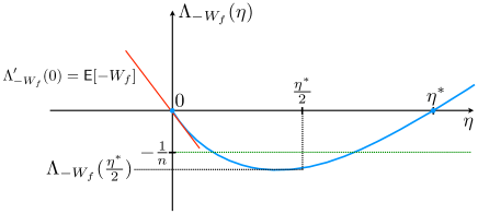
Figure 3: Control of the CGF of $-W_{f}$ for a function $f$ with excess loss $\operatorname*{{\bf E}}[W_{f}]$ of order $\frac{1}{n}$. The derivative at $0$ equals $-\operatorname*{{\bf E}}[W_{f}]$.

The general moment problem.

Let $\Delta(\mathcal{S})$ be the set of all probability measures over a measurable space $\mathcal{S}$. Then for any real-valued measurable functions $h$, $g_{1},\ldots,g_{m}$ on $\mathcal{S}$ and constants $k_{1},\ldots,k_{m}$, the general moment problem is the semi-infinite linear program

$$\begin{aligned} &\inf_{P\in\Delta(\mathcal{S})}&&\operatorname*{{\bf E}}_{S\sim P}h(S)\\ &\text{subject to}&&\operatorname*{{\bf E}}_{S\sim P}g_{j}(S)=k_{j},\quad j=1,\ldots,m.\end{aligned}$$ (48)

Define the vector-valued map $g\colon\mathcal{S}\to\mathbb{R}^{m}$ as $g(s)=(g_{1}(s),\ldots,g_{m}(s))$ and the vector $k=(k_{1},\ldots,k_{m})$. Then Theorem 3 of Kemperman (1968), which was also shown independently by Richter (1957) and Karlin and Studden (1966), states that, if $k\in\operatorname*{\mathrm{int}}\operatorname*{\operatorname{co}}(g(\mathcal{S}))$, the optimal value of problem (48) equals

$$\sup\biggl{\{}d_{0}+\sum_{j=1}^{m}d_{j}k_{j}:d^{*}=(d_{0},d_{1},\ldots,d_{m})\in D^{*}\biggr{\}},$$ (49)

where $D^{*}\subseteq\mathbb{R}^{m+1}$ is the set

$$D^{*}:=\biggl{\{}d^{*}=(d_{0},d_{1},\ldots,d_{m})\in\mathbb{R}^{m+1}:h(s)\geq d_{0}+\sum_{j=1}^{m}d_{j}g_{j}(s)\text{ for all }s\in\mathcal{S}\biggr{\}}.$$ (50)

Instantiating, we choose $\mathcal{S}=[-1,1]$ and define

$$h(s)=-e^{(\eta^{*}/2)s}, g_{1}(s)=s, g_{2}(s)=e^{\eta^{*}s}, k_{1}=-\frac{a}{n}, k_{2}=1,$$

which yields the following special case of problem (48):

$$\inf_{P\in\Delta([-1,1])} \quad-\operatorname*{{\bf E}}_{S\sim P}e^{(\eta^{*}/2)S}$$ (51a)

subject to $$\quad\operatorname*{{\bf E}}_{S\sim P}S=-\frac{a}{n}$$ (51b)

$$\quad\operatorname*{{\bf E}}_{S\sim P}e^{\eta^{*}S}=1.$$ (51c)

Equation 49 from the general moment problem now instantiates to

$$\sup\left\{d_{0}-\frac{a}{n}d_{1}+d_{2}:d^{*}=(d_{0},d_{1},d_{2})\in D^{*}\right\},$$ (52)

with $D^{*}$ equal to the set

$$\left\{d^{*}=(d_{0},d_{1},d_{2})\in\mathbb{R}^{3}:-e^{(\eta^{*}/2)s}\geq d_{0}+d_{1}x+d_{2}e^{\eta^{*}s}\text{ for all }s\in[-1,1]\right\}.$$ (53)

Applying Theorem 3 of Kemperman (1968) requires $k\in\operatorname*{\mathrm{int}}\operatorname*{\operatorname{co}}g([-1,1])$. We first characterize when $k\in\operatorname*{\operatorname{co}}g([-1,1])$ holds and handle the $\operatorname*{\mathrm{int}}\operatorname*{\operatorname{co}}g([-1,1])$ version after Theorem 7.53. The proof of the next result, along with all subsequent results in this section, can be found in Section A.4.

Lemma 7.52

For $a>0$, the point $k=\left(-\frac{a}{n},1\right)\in\operatorname*{\operatorname{co}}(g([-1,1]))$ if and only if

$$\frac{a}{n}\leq\frac{e^{\eta^{*}}+e^{-\eta^{*}}-2}{e^{\eta^{*}}-e^{-\eta^{*}}}=\frac{\cosh(\eta^{*})-1}{\sinh(\eta^{*})}.$$ (54)

Moreover, $k\in\operatorname*{\mathrm{int}}\operatorname*{\operatorname{co}}(g([-1,1]))$ if and only if the inequality in (54) is strict.

Note that (54) is guaranteed to hold, because otherwise the semi-infinite linear program (51) is infeasible (which in turn implies that such an excess loss random variable cannot exist).

The next theorem is a key result for using the strong central condition to control the CGF.

Theorem 7.53

Let $f$ be an element of $\mathcal{F}$ with $(\ell_{f}-\ell_{f^{*}})(Z)$ taking values in $[-1,1]$, $n\in\mathbb{N}$, $\operatorname*{{\bf E}}_{Z\sim P}(\ell_{f}-\ell_{f^{*}})(Z)=\frac{a}{n}$ for some $a>0$, and $\Lambda_{-(\ell_{f}-\ell_{f^{*}})(Z)}(\eta^{*})=0$ for some $\eta^{*}>0$. If

$$\frac{a}{n}<\frac{\cosh(\eta^{*})-1}{\sinh(\eta^{*})},$$ (55)

then $$\Lambda_{-(\ell_{f}-\ell_{f^{*}})(Z)}(\eta^{*}/2)\leq\frac{-0.21(\eta^{*}\operatorname*{\wedge}1)a}{n}.$$

Corollary 7.54

The result of Theorem 7.53 also holds when the strict inequality in (55) is replaced with inequality, i.e. $\frac{a}{n}\leq\frac{\cosh(\eta^{*})-1}{\sinh(\eta^{*})}$.

We now present an extension of this result for losses with range $[0,V]$.

Corollary 7.55

Let $g_{1}(x)=x$ and $y_{2}=1$ be common settings for the following two problems. The instantiation of problem (48) with $\mathcal{S}=[-V,V]$, $h(x)=-e^{(\eta/2)x}$, $g_{2}(x)=e^{\eta x}$, and $y_{1}=-\frac{a}{n}$ has the same optimal value as the instantiation of problem (48) with $\mathcal{S}=[-1,1]$, $h(x)=-e^{(V\eta/2)x}$, $g_{2}(x)=e^{(V\eta)x}$, and $y_{1}=-\frac{a/V}{n}$.

7.3 Fast Rates

We now show how the above results can be used to obtain an exact oracle inequality with a fast rate. We first present a result for finite classes and then present a result for VC-type classes (classes with logarithmic universal metric entropy).

Theorem 7.56

Let $(\ell,\operatorname{\mathit{P}},\mathcal{F})$ satisfy the strong $\eta^{*}$-central condition, where $|\mathcal{F}|=N$, $\ell$ is a nonnegative loss, and $\sup_{f\in\mathcal{F}}\ell_{f}(Z)\leq V$ a.s. for a constant $V$. Then for all $n\geq 1$, with probability at least $1-\delta$

$$\operatorname*{{\bf E}}_{Z\sim P}[\ell_{\hat{f}_{\mathbf{Z}}}(Z)]\leq\operatorname*{{\bf E}}_{Z\sim P}[\ell_{f^{*}}(Z)]+\frac{5\max\left\{V,\frac{1}{\eta^{*}}\right\}\left(\log\frac{1}{\delta}+\log N\right)}{n}.$$

Before presenting the result for VC-type classes, we require some definitions. For a pseudometric space $(\mathcal{G},d)$, for any $\varepsilon>0$, let $\mathcal{N}(\varepsilon,\mathcal{G},d)$ be the $\varepsilon$-covering number of $(\mathcal{G},d)$; that is, $\mathcal{N}(\varepsilon,\mathcal{G},d)$ is the minimal number of balls of radius $\varepsilon$ needed to cover $\mathcal{G}$. We will further constrain the cover (the set of centers of the balls) to be a subset of $\mathcal{G}$ (i.e. to be proper), thus ensuring that the strong central condition assumption transfers to any (proper) cover of $\mathcal{F}$. Note that the ‘proper’ requirement at most doubles the constant $K$ below, as shown in Lemma 2.1 of Vidyasagar (2002).

We now present the fast rates result for VC-type classes. The proof, which can be found as the proof of Theorem 7 of Mehta and Williamson (2014), uses Theorem 6 of Mehta and Williamson (2014) and the proof of Theorem 7.56. Below, we denote the loss-composed version of a function class $\mathcal{F}$ as $\ell\circ\mathcal{F}:=\{\ell_{f}:f\in\mathcal{F}\}$.

Theorem 7.57

Let $(\ell,\operatorname{\mathit{P}},\mathcal{F})$ satisfy the strong $\eta^{*}$-central condition with $\ell\circ\mathcal{F}$ separable, where, for a constant $K\geq 1$, for each $\varepsilon\in(0,K]$ we have $\mathcal{N}(\ell\circ\mathcal{F},L_{2}(\operatorname{\mathit{P}}),\varepsilon)\leq\left(\frac{K}{\varepsilon}\right)^{\mathcal{C}}$, and $\sup_{f\in\mathcal{F}}\ell\bigl{(}Y,f(X)\bigr{)}\leq V$ a.s. for a constant $V\geq 1$. Then for all $n\geq 5$ and $\delta\leq\frac{1}{2}$, with probability at least $1-\delta$,

$$\operatorname*{{\bf E}}_{Z\sim P}[\ell_{\hat{f}_{\mathbf{Z}}}(Z)]\leq\\ \operatorname*{{\bf E}}_{Z\sim P}[\ell_{f^{*}}(Z)]+\frac{1}{n}\max\left\{\begin{array}[]{c}8\max\left\{V,\frac{1}{\eta^{*}}\right\}\left(\mathcal{C}\log(Kn)+\log\frac{2}{\delta}\right),\\ 2V\left(1080\mathcal{C}\log(2Kn)+90\sqrt{\left(\log\frac{2}{\delta}\right)\mathcal{C}\log(2Kn)}+\log\frac{2e}{\delta}\right)\end{array}\right\}+\frac{1}{n}.$$ (56)

We have shown the fast rate of $O(1/n)$ under the best case of the $v$-central condition, i.e. when $v$ is constant; however, it also is possible to recover intermediate rates for the case of general $v$.

Corollary 7.58

Let $(\ell,\operatorname{\mathit{P}},\mathcal{F})$ satisfy the $v$-central condition hold for a finite class $\mathcal{F}$. Then, for some constant $c$, for all $n$ satisfying $v\left(w^{-1}\left(\frac{5(\log\frac{1}{\delta}+\log N)}{cn}\right)\right)\leq\frac{1}{cV}$, we get an intermediate rate of $w\left(\frac{5(\log\frac{1}{\delta}+\log N)}{cn}\right)$, where $w$ is the inverse of the function $x\mapsto xv(x)$.

Proof  From part (2) of Theorem 5.41, the $v$-central condition implies the $u$-Bernstein condition for $u(x)\asymp x/v(x)$, and from part (1b) of Theorem 5.41, we then have the $\eta$-central condition for $\eta=cv(\delta)$ for the subclass of functions with excess risk above $\delta$, for some constant $c$. From here, a simple modification of the proof of Theorem 7.56 yields the desired result as follows. Let $\varepsilon$ correspond to the excess risk threshold above which ERM should reject all functions with high probability. Then, similar to the proof of Theorem 7.56, we upper bound the probability of ERM picking a function with excess risk $\varepsilon$ or higher:

$$N\exp(n\Lambda_{-W_{f}}(cv(\varepsilon)) =N\exp(n\Lambda_{-W_{f}/V}(cVv(\varepsilon))$$

$$\leq N\exp\left(-0.21n\bigl{(}cVv(\varepsilon)\operatorname*{\wedge}1\bigr{)}\frac{\varepsilon}{V}\right).$$

For $\varepsilon$ satisfying $v(\varepsilon)\leq\frac{1}{cV}$, the failure probability $\delta$ is at most $N\exp(-0.21cn\varepsilon v(\varepsilon))$, and hence by inversion we get the rate $w\left(\frac{5(\log\frac{1}{\delta}+\log N)}{cn}\right)$.  

8 Discussion, Open Problems and Concluding Remarks

In this paper we identified four general conditions for fast and intermediate learning rates. The two main ones, which subsumed many previously identified conditions, where the central condition and stochastic mixability. We provided sufficient assumptions under which the four conditions become equivalent via the implications

$$\eta\text{-central}\Rightarrow\eta\text{-predictor}\Rightarrow\eta\text{-stochastic mixability}\Rightarrow\eta\text{-PPC}\Rightarrow\eta\text{-central}.$$ (57)

In Section 3 and 4 we considered the versions of these conditions for fixed $\eta>0$, as given by Theorem 4.33, Proposition 4.27, Proposition 4.28 and Theorem 3.13, respectively. For this fixed $\eta>0$ case, all implications except one hold under surprisingly weak conditions, in particular allowing for unbounded loss functions. The exception is ‘central $\Rightarrow$ predictor’ (Theorem 4.33). Although even this result was applicable to some noncompact decision sets $\mathcal{F}$ with unbounded losses (Example 4.37), it requires tightness and convexity of the set $\mathcal{P}$, although Example 4.34 shows that sometimes the implication holds even though $\mathcal{P}$ is neither tight nor convex. An important open question is whether Theorem 4.33 still holds under weaker versions of Assumption C or Assumption D.

Another restriction of Theorem 4.33 is that, via Assumption D, it requires convexity of the decision set $\mathcal{F}_{\textnormal{d}}$, which fails for the $0/1$-loss $\ell^{\textnormal{01}}$ and its conditional version, the classification loss $\ell^{\textnormal{class}}$. However, we may extend the definition of $\ell^{\textnormal{01}}$ to $\mathcal{F}=[0,1]$ and define the resulting randomized $0/1$ or absolute loss as $\ell^{\textnormal{abs}}_{f}(z):=|y-f|$. This can be interpreted as the $0/1$-loss a decision maker expects to make if she is allowed to randomize her decision by flipping a coin with bias $f$ — a standard concept in PAC-Bayesian approaches (Audibert, 2004; Catoni, 2007). For the absolute loss, we can consider $\eta$-stochastic mixability for $\mathcal{F}_{\textnormal{d}}=\operatorname*{\operatorname{co}}(\mathcal{F})=[0,1]$, which is convex; hence, the requirement of convex $\mathcal{F}_{\textnormal{d}}$ in Theorem 4.33 is not such a concern.

In Section 5 we discussed weakenings of the four conditions to their $v$-versions. Now for bounded losses, the four implications above still hold under similar conditions as for the fixed $\eta$-case. Since the first three implications in (57) were proven in an ‘up to $\varepsilon$’ form for all $\varepsilon>0$, it immediately follows that for arbitrary functions $v$, the implications continue to hold under the same assumptions if the $\eta$-conditions are replaced by the corresponding $v$-conditions. This does not work for the fourth implication, since Theorem 3.13 is not given in an ‘up to $\varepsilon$’ form (indeed, we conjecture that it does not hold in this form). However, we can work around this issue by using instead a detour via the Bernstein condition: by using first part 2 and then part 1 in Theorem 5.41, it follows that the $v$-PPC condition implies the $v^{\prime}$-central condition for $v^{\prime}(\varepsilon)\asymp v(\varepsilon)$, so the four $v$-conditions still imply each other, under the same assumptions as before, up to constant factors. However, the Bernstein-detour works only for bounded losses, and Example 5.44, 5.45 and 5.47 together indicate that in general it cannot be made to work and indeed the analogue of (57) for the $v$-conditions does not hold for unbounded losses: for decision problems with polynomial rather than exponential tails on the losses, $v$-stochastic mixability and the $v$-PPC condition may hold whereas the $v$-central condition does not. Thus there is the question whether the central condition can be weakened such that the four implications for the $v$-versions continue to hold, under weak conditions, for unbounded losses — and we regard this as the main open question posed by this work. Another issue here is that, if in a decision problem $(\ell,\mathcal{P},\mathcal{F})$ that satisfies a $v$-condition, we replace $\mathcal{P}$ by its convex closure, then the $v$-condition may very well be broken, so, once again, a weakening of Assumption D to nonconvex $\mathcal{P}$ seems required. Finally, it would be of considerable interest if one could show an analogue for unbounded losses of Proposition 5.48, which connects — for bounded losses — the central condition to the existence of a unique risk minimizer. Relatedly, it would be desirable to link this proposition to the results by Mendelson (2008a) who also connects slow rates with nonunique risk minimizers, and to Koltchinskii (2006) who gives a version of the Bernstein condition that does hold if nonunique minimizers exist, indicating that our $\eta$-central condition (which via Proposition 3.6 implies unique minimizers) might sometimes be too strong.

Apart from these implications in the ‘main quadrangle’ of Figure 1 on page 1, it would be good to strengthen some of the other connections shown in that figure, such as the precise relation between $\eta$-mixability and $\eta$-exp-concavity. It would also be desirable to establish connections to results in defensive forecasting (Chernov et al., 2010) in which conditions similar to both the central condition and mixability play a role; their Theorem 9 is reminiscent of the special case of our Theorem 4.33 for the case that $\mathcal{Z}$ is finite and $\mathcal{P}$ consists of all distributions on $\mathcal{Z}$.

We focused on showing equivalence of fast rate conditions and not on showing that one can actually always obtain fast rates under these conditions. For stochastic mixability, this immediately follows, under no further conditions, from Proposition 4.21. For the central condition, the situation is more complicated: in this paper we only showed that it implies fast rates for bounded loss functions. We know that, for the unbounded log-loss, fast rates can be obtained under the central condition (and no additional conditions) in a weaker sense, involving Rényi and squared Hellinger distance (Section 2.2); in work in progress, we aim at showing that the central condition implies fast rates in the standard sense even for unbounded loss functions. This does appear possible, up to log-factors, however it seems that here one does need weak additional conditions such as existence of certain moments different from the exponential moment in (4).

Second, by ‘fast’ rates we merely meant rates of order $1/n$; it would of course be highly desirable to characterize when the rates that are achieved under our conditions by appropriate algorithms (ERM, Bayes MAP-style and MDL methods for the central condition, the aggregating algorithm for stochastic mixability) are indeed minimax optimal. Similarly, one would need examples showing that if a condition fails, then the corresponding fast or intermediate rates cannot be obtained in general. While several such results are available, they either focus on showing that, in the worst-case over all $P\in\mathcal{P}$, no learning algorithm, proper or improper, can achieve a certain rate (in particular Audibert (2009) gives very general results), or that a particular proper learning algorithm such as ERM cannot achieve a certain rate (Mendelson, 2008a). Currently unexplored, it seems, are minimax results where one looks at the optimal (not just ERM) algorithm, but within the restricted class of all proper learning algorithms.

In the spirit of Vapnik and Chervonenkis, who discovered under what conditions one can learn from a finite amount of data at all, we continue our quest for conditions under which one can learn from data using not too many examples.

Acknowledgments

We thank Olivier Catoni for raising the issue of unbounded losses discussed in Example 5.44, Wouter Koolen for suggesting the connection to minimax theorems, and Andrew Barron for various in-depth discussions over the last 16 years. Most of the results in Section 7 were published before in the conference paper by Mehta and Williamson (2014); very preliminary versions of Theorem 3.13, Theorem 4.33 (only for $\mathcal{P}$ the set of all distributions on $\mathcal{Z}$) and Theorem 5.41 were published before by van Erven et al. (2012a), in which we used the phrase ‘$(\ell,\mathcal{P},\mathcal{F})$ is stochastically mixable’ to denote what we now refer to as ‘$(\ell,\mathcal{P},\mathcal{F})$ satisfies the central condition’. We thank both the referees of the present paper and the referees of these earlier conference papers for their useful feedback. This work was supported in part by the Australian Research Council, and by NICTA which is funded by the Australian Government, as well as by by the Netherlands Organiszation for Scientific Research (NWO) Project 639.073.904.

A Additional Proofs

A.1 Proof of Theorem 3.13 in Section 3

Proof  We first consider the case that Assumption A holds, and then the case of bounded loss.

Under Assumption A.

Under our Assumption A, we can, for each $P\in\mathcal{P}$, define $\phi(P):=f^{*}\in\mathcal{F}$ to be optimal in the sense of (3). Note that $f^{*}$ depends on $P$, but not on any $\Pi$. Since we also assume the weak $\eta$-pseudoprobability convexity condition, we must have that for every $\varepsilon>0$, the $\eta$-pseudoprobability convexity condition holds up to $\varepsilon$ for some function $\phi_{\varepsilon}$. It follows that for all $\varepsilon>0$, $\operatorname*{{\bf E}}_{Z\sim P}[\ell_{f^{*}}(Z)]\leq\operatorname*{{\bf E}}_{Z\sim P}[\ell_{\phi_{\varepsilon}(P)}(Z)]\leq\operatorname*{{\bf E}}_{Z\sim P}[m_{\Pi}^{\eta}(Z)]+\varepsilon$, so that also

$$\operatorname*{{\bf E}}_{Z\sim P}[\ell_{f^{*}}(Z)]\leq\operatorname*{{\bf E}}_{Z\sim P}[m_{\Pi}^{\eta}(Z)]$$ (58)

for all $\Pi\in\Delta(\mathcal{F})$. Now fix arbitrary $P\in\mathcal{P}$, let $f^{*}=\phi(P)$ and let $f\in\mathcal{F}$ be arbitrary and consider the special case that $\Pi=(1-\lambda)\delta_{f^{*}}+\lambda\delta_{f}$ for $\lambda\in[0,\tfrac{1}{2}]$, where $\delta_{f}$ is a point-mass on $f$. Let

$$\chi(\lambda,z)=\eta m_{\Pi}^{\eta}(z)=-\log\left((1-\lambda)e^{-\eta\ell_{f^{*}}(z)}+\lambda e^{-\eta\ell_{f}(z)}\right)$$

be the corresponding mix loss multiplied by $\eta$, and let

$$\chi(\lambda)=\operatorname*{{\bf E}}_{Z\sim P}[\chi(\lambda,Z)]=\eta\operatorname*{{\bf E}}_{Z\sim P}[m_{\Pi}^{\eta}(Z)]$$

be its expected value. Then from (58) it follows that $\chi(\lambda)$ is minimized at $\lambda=0$, which implies that the right-derivative $\chi^{\prime}(0)$ at $0$ is nonnegative:

$$\chi^{\prime}(0)\geq 0.$$ (59)

In order to compute $\chi^{\prime}(0)$, we first observe that, for any $z$, $\chi(\lambda,z)$ is convex in $\lambda$, because it is the composition of the negative logarithm with a linear function. Convexity of $\chi(\lambda,z)$ in $\lambda$ implies that the slope $s(d,z)=\frac{\chi(0+d,z)-\chi(0,z)}{d}$ is non-decreasing in $d\in(0,\tfrac{1}{2}]$ and achieves its maximum value at $d=1/2$, where it never exceeds $2\log 2$:

$$s(1/2,z)=2\log\frac{e^{-\eta\ell_{f^{*}}(z)}}{\frac{1}{2}e^{-\eta\ell_{f^{*}}(z)}+\frac{1}{2}e^{-\eta\ell_{f}(z)}}\leq 2\log\frac{e^{-\eta\ell_{f^{*}}(z)}}{\frac{1}{2}e^{-\eta\ell_{f^{*}}(z)}}=2\log 2.$$

Hence $\operatorname*{{\bf E}}_{Z\sim P}[s(\frac{1}{2},Z)]\leq 2\log 2<\infty$ and by the monotone convergence theorem (Shiryaev, 1996)

$$\chi^{\prime}(0)=\lim_{d\downarrow 0}\operatorname*{{\bf E}}_{Z\sim P}\left[s(d,Z)\right]=\operatorname*{{\bf E}}_{Z\sim P}\left[\lim_{d\downarrow 0}s(d,Z)\right]=\operatorname*{{\bf E}}_{Z\sim P}\left[\frac{\mathrm{d}}{\mathrm{d}\lambda}\chi(\lambda,Z)|_{\lambda=0}\right]=1-\operatorname*{{\bf E}}_{Z\sim P}\left[\frac{e^{-\eta\ell_{f}(Z)}}{e^{-\eta\ell_{f^{*}}(Z)}}\right].$$ (60)

Together with (59) and the fact that $\phi(P)=f^{*}$ and that $P$ was chosen arbitrarily, this implies the strong $\eta$-central condition as required.

When the Loss is Bounded.

Let $P\in\mathcal{P}$ be arbitrary. The $\eta$-pseudoprobability convexity condition implies that for any $\gamma>0$ we can find $f^{*}\in\mathcal{F}$ such that

$$\operatorname*{{\bf E}}_{Z\sim P}\left[\ell_{f^{*}}(Z)\right]\leq\operatorname*{{\bf E}}_{Z\sim P}\left[m_{\Pi}^{\eta}(Z)\right]+\gamma$$

for all distributions $\Pi\in\Delta(\mathcal{F})$. Choose any $f\in\mathcal{F}$ and consider again the special case $\Pi=(1-\lambda)\delta_{f^{*}}+\lambda\delta_{f}$ for $\lambda\in[0,\tfrac{1}{2}]$, which gives

$$\chi(0)\leq\chi(\lambda)+\eta\gamma$$ (61)

for $\chi(\lambda)$ as above. This time $\chi(0)$ is not necessarily the exact minimum of $\chi(\lambda)$, but (61) expresses that it is close. To control $\chi^{\prime}(0)$, we use that

$$\chi(\lambda,z)=\chi(0,z)+\lambda\tfrac{\mathrm{d}}{\mathrm{d}\lambda}\chi(0,z)+\tfrac{1}{2}\lambda^{2}\tfrac{\mathrm{d}^{2}}{\mathrm{d}\lambda^{2}}\chi(\xi,z)\qquad\text{for some $\xi\in[0,\lambda]$}$$

by a second-order Taylor expansion in $\lambda$, which implies that

$$\chi(\lambda)-\chi(0)-\lambda\chi^{\prime}(0)\leq\frac{\lambda^{2}}{2}\max_{z,\lambda^{\prime}}\left(\frac{e^{-\eta\ell_{f^{*}}(z)}-e^{-\eta\ell_{f}(z)}}{(1-\lambda^{\prime})e^{-\eta\ell_{f^{*}}(z)}+\lambda^{\prime}e^{-\eta\ell_{f}(z)}}\right)^{2}\leq\frac{\lambda^{2}}{2}\left(e^{\eta 2B}-1\right)^{2}.$$

Together with (61) the choice $\lambda=\sqrt{\gamma}$ (which requires $\gamma\leq 1/4$) then allows us to conclude that

$$-\eta\gamma \leq\chi(\sqrt{\gamma})-\chi(0)\leq\sqrt{\gamma}\chi^{\prime}(0)+\frac{\gamma}{2}\left(e^{\eta 2B}-1\right)^{2}$$

$$\chi^{\prime}(0) \geq-c\sqrt{\gamma}$$

for $c=\eta+\frac{1}{2}(e^{\eta 2B}-1)^{2}$. Since (60) still holds, taking $\gamma$ small enough that $1+c\sqrt{\gamma}\leq e^{\eta\varepsilon}$ gives us the central condition (12) for any $\varepsilon>0$.  

A.2 Proof of Lemma 4.32 in Section 4

Proof  Theorem 6.1 of Grünwald and Dawid (2004), itself a direct consequence of a minimax theorem due to Ferguson (1967), states the following: if a set of distributions $\bar{\mathcal{P}}$ is convex, tight and closed in the weak topology, and $L\colon\mathcal{Z}\times\mathcal{F}_{\textnormal{d}}\to\mathbb{R}$ is a function such that, for all $f$, $L(z,f)$ is bounded from above and upper semi-continuous in $z$, then

$$\sup_{P\in\bar{\mathcal{P}}}\operatorname*{\vphantom{p}inf}_{f\in\mathcal{F}_{\textnormal{d}}}\operatorname*{{\bf E}}_{Z\sim P}[L(Z,f)]=\operatorname*{\vphantom{p}inf}_{\rho\in\Delta(\mathcal{F}_{\textnormal{d}})}\sup_{P\in\bar{\mathcal{P}}}\operatorname*{{\bf E}}_{Z\sim P}\operatorname*{{\bf E}}_{f\sim\rho}[L(Z,f)].$$ (62)

Let $\Pi\in\Delta(\mathcal{F}_{\textnormal{d}})$ be arbitrary, and observe that $S_{\Pi}^{\eta}(P,f)$ is related to $\xi_{Z,f}$ via

$$S_{\Pi}^{\eta}(P,f)=\operatorname*{{\bf E}}_{Z\sim P}[\xi_{Z,f}],$$

so we will aim to apply (62) with $L(z,f)$ approximately equal to $\xi_{z,f}$. Although $\xi_{z,f}$ is not necessarily bounded above, rewriting

$$\xi_{z,f}=e^{\eta\ell_{f}(z)}\operatorname*{{\bf E}}_{g\sim\Pi}\left[e^{-\eta\ell_{g}(z)}\right],$$

we find that it is continuous in $z$, because $\ell_{f}(z)$ is continuous in $z$ and $\operatorname*{{\bf E}}_{g\sim\Pi}\left[e^{-\eta\ell_{g}(z)}\right]$ is also continuous in $z$ by continuity of $\ell_{g}(z)$ and the dominated convergence theorem (Shiryaev, 1996), which applies because $|e^{-\eta\ell_{g}(z)}|\leq 1$. Letting $a\operatorname*{\wedge}b$ denote the minimum of $a$ and $b$, it follows that $\xi_{z,f}\operatorname*{\wedge}b$ is also continuous in $z$ for any number $b$.

Thus we can apply (62) to the function $L(z,f)=\xi_{z,f}\operatorname*{\wedge}b$, with $\bar{\mathcal{P}}$ the closure of $\mathcal{P}$ in the weak topology, to obtain

$$\operatorname*{\vphantom{p}inf}_{\rho\in\Delta(\mathcal{F}_{\textnormal{d}})}\sup_{P\in{\mathcal{P}}}\operatorname*{{\bf E}}_{Z\sim P}\operatorname*{{\bf E}}_{f\sim\rho}[\xi_{Z,f}\operatorname*{\wedge}b]\leq\operatorname*{\vphantom{p}inf}_{\rho\in\Delta(\mathcal{F}_{\textnormal{d}})}\sup_{P\in{\bar{\mathcal{P}}}}\operatorname*{{\bf E}}_{Z\sim P}\operatorname*{{\bf E}}_{f\sim\rho}[\xi_{Z,f}\operatorname*{\wedge}b]=\sup_{P\in{\bar{\mathcal{P}}}}\operatorname*{\vphantom{p}inf}_{f\in\mathcal{F}_{\textnormal{d}}}\operatorname*{{\bf E}}_{Z\sim P}[\xi_{Z,f}\operatorname*{\wedge}b].$$ (63)

We will show that

$$\sup_{P\in{\bar{\mathcal{P}}}}\operatorname*{\vphantom{p}inf}_{f\in\mathcal{F}_{\textnormal{d}}}\operatorname*{{\bf E}}_{Z\sim P}[\xi_{Z,f}\operatorname*{\wedge}b]\leq\sup_{P\in\mathcal{P}}\operatorname*{\vphantom{p}inf}_{f\in\mathcal{F}_{\textnormal{d}}}\operatorname*{{\bf E}}_{Z\sim P}[\xi_{Z,f}\operatorname*{\wedge}b].$$ (64)

If $\mathcal{P}$ is closed itself (first possibility in D.4), then $\bar{\mathcal{P}}=\mathcal{P}$ and this is immediate. The second possibility will be covered at the end of the proof.

Together, (63) and (64) imply that

$$\operatorname*{\vphantom{p}inf}_{\rho\in\Delta(\mathcal{F}_{\textnormal{d}})}\sup_{P\in{\mathcal{P}}}\operatorname*{{\bf E}}_{Z\sim P}\operatorname*{{\bf E}}_{f\sim\rho}[\xi_{Z,f}\operatorname*{\wedge}b]\leq\sup_{P\in\mathcal{P}}\operatorname*{\vphantom{p}inf}_{f\in\mathcal{F}_{\textnormal{d}}}\operatorname*{{\bf E}}_{Z\sim P}[\xi_{Z,f}\operatorname*{\wedge}b]\leq\sup_{P\in\mathcal{P}}\operatorname*{\vphantom{p}inf}_{f\in\mathcal{F}_{\textnormal{d}}}\operatorname*{{\bf E}}_{Z\sim P}[\xi_{Z,f}]$$

for any finite $b$. We will show that, for every $\varepsilon>0$, there exists a $b$ such that

$$\operatorname*{{\bf E}}_{Z\sim P}\operatorname*{{\bf E}}_{f\sim\rho}[\xi_{Z,f}\operatorname*{\wedge}b]\geq\operatorname*{{\bf E}}_{Z\sim P}\operatorname*{{\bf E}}_{f\sim\rho}[\xi_{Z,f}]-\varepsilon\qquad\text{for all $\rho\in\Delta(\mathcal{F}_{\textnormal{d}})$ and $P\in{\mathcal{P}}$.}$$ (65)

By letting $\varepsilon$ tend to $0$, we can therefore conclude that

$$\sup_{P\in{\mathcal{P}}}\operatorname*{\vphantom{p}inf}_{f\in\mathcal{F}_{\textnormal{d}}}\operatorname*{{\bf E}}_{Z\sim P}[\xi_{Z,f}]\geq\operatorname*{\vphantom{p}inf}_{\rho\in\Delta(\mathcal{F}_{\textnormal{d}})}\sup_{P\in{\mathcal{P}}}\operatorname*{{\bf E}}_{Z\sim P}\operatorname*{{\bf E}}_{f\sim\rho}[\xi_{Z,f}]=\operatorname*{\vphantom{p}inf}_{f\in\mathcal{F}_{\textnormal{d}}}\sup_{P\in{\mathcal{P}}}\operatorname*{{\bf E}}_{Z\sim P}[\xi_{Z,f}],$$ (66)

where the identity follows from the requirement that $e^{\eta\ell_{f}(z)}$ is convex in $f$, which implies that $\xi_{Z,f}$ is also convex in $f$, and hence the mean of $\rho$ is always at least as good as $\rho$ itself: $\xi_{Z,\operatorname*{{\bf E}}_{f\sim\rho}[f]}\leq\operatorname*{{\bf E}}_{f\sim\rho}[\xi_{Z,f}]$. Since the $\sup\inf$ never exceeds the $\inf\sup$, (66) implies (32), which was to be shown.

To prove (65), we observe that

$$\operatorname*{{\bf E}}_{Z\sim P}\operatorname*{{\bf E}}_{f\sim\rho}[\xi_{Z,f}\operatorname*{\wedge}b]\geq\operatorname*{{\bf E}}_{Z\sim P}\operatorname*{{\bf E}}_{f\sim\rho}[\xi_{Z,f}\mathop{\llbracket\xi_{Z,f}<b\rrbracket}]\\ =\operatorname*{{\bf E}}_{Z\sim P}\operatorname*{{\bf E}}_{f\sim\rho}[\xi_{Z,f}]-\operatorname*{{\bf E}}_{Z\sim P}\operatorname*{{\bf E}}_{f\sim\rho}[\xi_{Z,f}\mathop{\llbracket\xi_{Z,f}\geq b\rrbracket}],$$

and, by uniform integrability, we can take $b$ large enough that $\operatorname*{{\bf E}}_{Z\sim P}\operatorname*{{\bf E}}_{f\sim\rho}[\xi_{Z,f}\mathop{\llbracket\xi_{Z,f}\geq b\rrbracket}]\leq\varepsilon$ for all $\rho$ and $P$, as required.

Finally, it remains to establish (64) for the second possibility in Assumption D.4. To this end, let $\varepsilon>0$ be arbitrary and let $\mathcal{Z}^{\prime}\subseteq\mathcal{Z}$ be a compact set such that $P(\mathcal{Z}^{\prime})\geq 1-\varepsilon$ for all $P\in\mathcal{P}$. In addition, let $\delta>0$ be small enough that

$$\sup_{z\in\mathcal{Z}^{\prime}}|\ell_{f}(z)-\ell_{g}(z)|<\varepsilon\qquad\text{for all $f,g\in\mathcal{F}_{\textnormal{d}}$ such that $d(f,g)<\delta$,}$$

which is possible by the assumption of uniform equicontinuity. Since $\mathcal{F}_{\textnormal{d}}$ is totally bounded, it can be covered by a finite number of balls of radius $\delta$. Let $\ddot{\mathcal{F}}_{\textnormal{d}}\subseteq\mathcal{F}_{\textnormal{d}}$ be the (finite) set of centers of those balls. Then we can bound the left-hand side of (64) as follows:

$$\sup_{P\in{\bar{\mathcal{P}}}}\operatorname*{\vphantom{p}inf}_{f\in\mathcal{F}_{\textnormal{d}}}\operatorname*{{\bf E}}_{Z\sim P}[L(Z,f)]\leq\sup_{P\in{\bar{\mathcal{P}}}}\min_{f\in\ddot{\mathcal{F}}_{\textnormal{d}}}\operatorname*{{\bf E}}_{Z\sim P}[L(Z,f)]=\sup_{P\in{\mathcal{P}}}\min_{f\in\ddot{\mathcal{F}}_{\textnormal{d}}}\operatorname*{{\bf E}}_{Z\sim P}[L(Z,f)],$$

where the equality holds by continuity of $\operatorname*{{\bf E}}_{Z\sim P}[L(Z,f)]$ and hence $\min_{f\in\ddot{\mathcal{F}}_{\textnormal{d}}}\operatorname*{{\bf E}}_{Z\sim P}[L(Z,f)]$ in $P$. We now need to relate $\ddot{\mathcal{F}}_{\textnormal{d}}$ back to $\mathcal{F}_{\textnormal{d}}$, which is possible because, for every $f\in\mathcal{F}_{\textnormal{d}}$, there exists $\ddot{f}\in\ddot{\mathcal{F}}_{\textnormal{d}}$ such that $d(f,\ddot{f})<\delta$ and hence $|\ell_{\ddot{f}}(z)-\ell_{f}(z)|<\varepsilon$ for all $z\in\mathcal{Z}^{\prime}$. It follows that $L(z,\ddot{f})\leq e^{\eta\varepsilon}L(z,f)$ and therefore

$$\sup_{P\in{\mathcal{P}}}\min_{f\in\ddot{\mathcal{F}}_{\textnormal{d}}}\operatorname*{{\bf E}}_{Z\sim P}[L(Z,f)]\leq\sup_{P\in{\mathcal{P}}}\min_{f\in\ddot{\mathcal{F}}_{\textnormal{d}}}\operatorname*{{\bf E}}_{Z\sim P}[\mathop{\llbracket Z\in\mathcal{Z}^{\prime}\rrbracket}L(Z,f)]+\varepsilon b\\ \leq e^{\eta\varepsilon}\sup_{P\in{\mathcal{P}}}\operatorname*{\vphantom{p}inf}_{f\in\mathcal{F}_{\textnormal{d}}}\operatorname*{{\bf E}}_{Z\sim P}[\mathop{\llbracket Z\in\mathcal{Z}^{\prime}\rrbracket}L(Z,f)]+\varepsilon b\leq e^{\eta\varepsilon}\sup_{P\in{\mathcal{P}}}\operatorname*{\vphantom{p}inf}_{f\in\mathcal{F}_{\textnormal{d}}}\operatorname*{{\bf E}}_{Z\sim P}[L(Z,f)]+\varepsilon b,$$

and letting $\varepsilon$ tend to $0$ we obtain (64), which completes the proof.  

A.3 Proof of Theorem 5.41 in Section 5

Proof  We prove the two cases in turn.

Bernstein $\Rightarrow$ Central.

Fix arbitrary $P\in\mathcal{P}$, and let $f^{*}$ be $\mathcal{F}$-optimal, i.e. satisfying (3). In this part of the proof, all expectations $\operatorname*{{\bf E}}$ are taken over $Z\sim P$.

Suppose that the $u$-Bernstein condition holds. Fix arbitrary $f\in\mathcal{F}$ and let $X=\ell_{f}(Z)-\ell_{f^{*}}(Z)$. Let $\varepsilon\geq 0$ and set $\eta=v(\varepsilon)\leq c_{1}^{b}\varepsilon/u(\varepsilon)$. We deal with $\varepsilon=0$ later and for now focus on the case $\varepsilon>0$, which implies $\eta>0$. Then Lemma 5.43, applied to the random variable $\eta X$, gives

$$\operatorname*{{\bf E}}[X]+\frac{1}{\eta}\log\operatorname*{{\bf E}}[e^{-\eta X}]\leq\kappa(2ba)\eta\operatorname*{{\bf Var}}(X)\leq\kappa(2ba)\eta u(\operatorname*{{\bf E}}[X])\leq\frac{\varepsilon}{u(\varepsilon)}u(\operatorname*{{\bf E}}[X]).$$

If $\varepsilon\leq\operatorname*{{\bf E}}[X]$, then the assumption that $\frac{u(\varepsilon)}{\varepsilon}$ is non-increasing in $\varepsilon$ implies that

$$\frac{\varepsilon}{u(\varepsilon)}u(\operatorname*{{\bf E}}[X])\leq\frac{\operatorname*{{\bf E}}[X]}{u(\operatorname*{{\bf E}}[X])}u(\operatorname*{{\bf E}}[X])=\operatorname*{{\bf E}}[X],$$ (67)

and we can conclude that $\frac{1}{\eta}\log\operatorname*{{\bf E}}[e^{-\eta X}]\leq 0\leq\varepsilon$. This inequality establishes (b), and it establishes (a) for the case $0<\varepsilon\leq\operatorname*{{\bf E}}[X]$. If $\varepsilon>\operatorname*{{\bf E}}[X]$, then the assumption that $u$ is non-decreasing implies that

$$\frac{\varepsilon}{u(\varepsilon)}u(\operatorname*{{\bf E}}[X])\leq\frac{\varepsilon}{u(\operatorname*{{\bf E}}[X])}u(\operatorname*{{\bf E}}[X])=\varepsilon,$$ (68)

and, using that $\operatorname*{{\bf E}}[X]\geq 0$, we again find that $\frac{1}{\eta}\log\operatorname*{{\bf E}}[e^{-\eta X}]\leq\varepsilon$, as required for (a). To finish the proof of (a) we now consider $\varepsilon=0$. If we also have $v(0)=0$ then the central condition (12) holds trivially for $\varepsilon=0$, so we may assume without loss of generality that $v(0)>0$. Then we must have $\eta=v(0)=\liminf_{x\downarrow 0}x/u(x)>0$. Now fix a decreasing sequence $\{\varepsilon_{j}\}_{j=1,2,\ldots}$ tending to $0$, where the $\varepsilon_{j}$ are all positive and let $\eta_{j}=v(\varepsilon_{j})$. By the argument above, the $\eta_{j}$-central condition holds up to $\varepsilon_{j}$. This implies (Fact 3.7) that for all $j$, all $\eta\leq\eta_{j}$, in particular for $\eta=v(0)$, the $\eta$-central condition also holds up to $\varepsilon_{j}$. Thus, the $\eta$-central condition holds up to $\varepsilon$ for all $\varepsilon>0$. By Proposition 3.14 it then follows that the strong $\eta$-central condition holds, i.e. it also holds for $\varepsilon=0$.

Pseudoprobability $\Rightarrow$ Bernstein.

Suppose that the $v$-PPC condition holds. Fix some $\varepsilon\geq 0$ and let $\eta=v(\varepsilon)$. Fix arbitrary $P\in\mathcal{P}$ and let $f^{*}$ be $\mathcal{F}$-optimal for $P$, achieving (3). Fix arbitrary $f\in\mathcal{F}$ and let $\Pi$ be the distribution on $\mathcal{F}$ assigning mass $1/2$ to $f^{*}$ and mass $1/2$ to $f$, and let $\bar{f}\in\{f,f^{*}\}$ be the corresponding random variable. For $z\in\mathcal{Z}$, let $Y_{z,\bar{f}}=\eta(\ell_{\bar{f}}(z)-\ell_{f^{*}}(z))$ and let $\varepsilon_{z}=\eta^{-1}\log\operatorname*{{\bf E}}_{\bar{f}\sim\Pi}\left[e^{-Y_{z,\bar{f}}}\right]$. Note that $Y_{z,\bar{f}}$ is a random variable under distribution $\Pi$ (not $P$, since $z$ is fixed), and that

$$\operatorname*{{\bf E}}_{\bar{f}\sim\Pi}[Y_{z,\bar{f}}]=\frac{1}{2}\eta\left(\ell_{f}(z)-\ell_{f^{*}}(z)\right).$$ (69)

Lemma 5.43 then gives, for each $z\in\mathcal{Z}$,

$$\kappa(-2ab)\operatorname*{{\bf Var}}_{\bar{f}\sim\Pi}[Y_{z,\bar{f}}]\leq\operatorname*{{\bf E}}_{\bar{f}\sim\Pi}[Y_{z,\bar{f}}]+\log\operatorname*{{\bf E}}_{\bar{f}\sim\Pi}\left[e^{-Y_{z,\bar{f}}}\right]=\frac{1}{2}\eta\left(\ell_{f}(z)-\ell_{f^{*}}(z)\right)+\eta\varepsilon_{z},$$ (70)

where we used the definition of $\Pi$ and $\varepsilon_{z}$. We may assume from the definition of the $v$-pseudoprobability convexity condition that (15) holds for the given $\varepsilon$ and $\eta$ and $\Pi$; rearranging this equation it is seen to be equivalent to $\operatorname*{{\bf E}}_{Z\sim P}[\varepsilon_{Z}]\leq\varepsilon.$ By taking expectations over $Z$ on both sides of (70) this gives

$$\kappa(-2ab)\operatorname*{{\bf E}}_{Z\sim P}\operatorname*{{\bf Var}}_{\bar{f}\sim\Pi}\left[Y_{Z}\right]\leq\frac{1}{2}\eta\operatorname*{{\bf E}}_{Z\sim P}\left[\ell_{f}(Z)-\ell_{f^{*}}(Z)\right]+\eta\varepsilon.$$ (71)

The $\Pi$-variance on the left can be rewritten, using (69), as

$$\operatorname*{{\bf Var}}_{\bar{f}\sim\Pi}\left[Y_{z,\bar{f}}\right] =\frac{1}{2}\left(\eta(\ell_{{f}}(z)-\ell_{f^{*}}(z))-\operatorname*{{\bf E}}_{\bar{f}\sim\Pi}\left[Y_{z,\bar{f}}\right]\right)^{2}+\frac{1}{2}\left(\eta\cdot 0-\operatorname*{{\bf E}}_{\bar{f}\sim\Pi}\left[Y_{z,\bar{f}}\right]\right)^{2}$$

$$=\frac{1}{2}\left(\frac{1}{2}\eta(\ell_{{f}}(z)-\ell_{f^{*}}(z))\right)^{2}+\frac{1}{2}\left(-\frac{1}{2}\eta(\ell_{{f}}(z)-\ell_{f^{*}}(z))\right)^{2}=\frac{1}{4}\eta^{2}(\ell_{{f}}(z)-\ell_{f^{*}}(z))^{2}.$$

Plugging this into (71) and dividing both sides by $\eta^{2}/(4\kappa(-2ab))$ gives

$$\operatorname*{{\bf E}}_{Z\sim P}(\ell_{{f}}(Z)-\ell_{f^{*}}(Z))^{2}\leq\frac{2}{\kappa(-2ab)\cdot\eta}\left(\operatorname*{{\bf E}}_{Z\sim P}\left[\ell_{f}(Z)-\ell_{f^{*}}(Z)\right]+2\varepsilon\right).$$ (72)

This holds for all $\varepsilon\geq 0$ and $\eta=v(\varepsilon)$, as long as $\eta=u(\varepsilon)>0$ (if $\eta=0$ we cannot divide by $\eta^{2}$ to go from (71) to (72)). Thus, we may set $\varepsilon=\operatorname*{{\bf E}}_{Z\sim P}\left[\ell_{f}(Z)-\ell_{f^{*}}(Z)\right]\geq 0$; if $\eta=u(\varepsilon)>0$ then (72) must hold for $\varepsilon$. With these values the right-hand side becomes $6\eta^{-1}\kappa^{-1}(2ab)\varepsilon=c_{2}\varepsilon/v(\varepsilon)=u(\varepsilon),$ and the result follows by our choice of $\varepsilon$. It remains to deal with the case $\eta=0$, which by definition of $v$ can only happen if $\varepsilon=\operatorname*{{\bf E}}_{Z\sim P}\left[\ell_{f}(Z)-\ell_{f^{*}}(Z)\right]=0$. In this case, (72) still holds for all values of $\varepsilon>0$. We thus infer that the left-hand side of (72) is bounded by $\inf_{\varepsilon>0}4\varepsilon/(\kappa(-2ab)v(\varepsilon)$, and the result follows by our definition of $0/v(0)$.  

A.4 Proofs for Section 7

Lemma A.59

(Hyper-Concentrated Excess Losses) Let $Z$ be a random variable with probability measure $P$ supported on $[-V,V]$. Suppose that $\lim_{\eta\rightarrow\infty}\operatorname*{{\bf E}}[\exp(-\eta Z)]<1$ and $\operatorname*{{\bf E}}[Z]=\mu>0$. Then there is a suitable modification $Z^{\prime}$ of $Z$ for which $Z^{\prime}\leq Z$ with probability 1, the mean of $Z^{\prime}$ is arbitrarily close to $\mu$, and $\operatorname*{{\bf E}}[\exp(-\eta Z^{\prime})]=1$ for arbitrarily large $\eta$.

Proof  First, observe that $Z\geq 0$ a.s. If not, then there must be some finite $\eta>0$ for which $\operatorname*{{\bf E}}[\exp(-\eta Z)]=1$. Now, consider a random variable $Z^{\prime}$ with probability measure $Q_{\varepsilon}$, a modification of $Z$ (with probability measure $P$) constructed in the following way. Define $A:=[\mu,V]$ and $A^{-}:=[-V,-\mu]$. Then for any $\varepsilon>0$ we define $Q_{\varepsilon}$ as

$${\mathrm{d}}Q_{\varepsilon}(z)=\begin{cases}(1-\varepsilon){\mathrm{d}}P(z)&\text{if }z\in A\\ \varepsilon{\mathrm{d}}P(-z)&\text{if }z\in A^{-}\\ {\mathrm{d}}P(z)&\text{otherwise}.\end{cases}$$

Additionally, we couple $P$ and $Q_{\varepsilon}$ such that the couple $(Z,Z^{\prime})$ is a coupling of $(P,Q_{\varepsilon})$ satisfying

$$\operatorname*{{\bf E}}_{(Z,Z^{\prime})\sim(P,Q_{\varepsilon})}\mathop{\llbracket Z\neq Z^{\prime}\rrbracket}=\min_{(P^{\prime},Q_{\varepsilon}^{\prime})}\operatorname*{{\bf E}}_{(Z,Z^{\prime})\sim(P^{\prime},Q_{\varepsilon}^{\prime})}\mathop{\llbracket Z\neq Z^{\prime}\rrbracket},$$

where the $\min$ is over all couplings of $P$ and $Q_{\varepsilon}$. This coupling ensures that $Z^{\prime}\leq Z$ with probability 1; i.e. $Z^{\prime}$ is dominated by $Z$.

Now,

$$\operatorname*{{\bf E}}[\exp(-\eta Z^{\prime})] =\int_{-V}^{V}e^{-\eta z}{\mathrm{d}}Q_{\varepsilon}(z)$$

$$=\int_{A^{-}}e^{-\eta z}{\mathrm{d}}Q_{\varepsilon}(z)+\int_{A}e^{-\eta z}{\mathrm{d}}Q_{\varepsilon}(z)+\int_{[0,V]\setminus A}e^{-\eta z}{\mathrm{d}}Q_{\varepsilon}(z)$$

$$=\varepsilon\int_{A^{-}}e^{-\eta z}{\mathrm{d}}P(-z)+(1-\varepsilon)\int_{A}e^{-\eta z}{\mathrm{d}}P(z)+\int_{[0,V]\setminus A}e^{-\eta z}{\mathrm{d}}P(z)$$

$$=\varepsilon\int_{A}e^{\eta z}{\mathrm{d}}P(z)+(1-\varepsilon)\int_{A}e^{-\eta z}{\mathrm{d}}P(z)+\int_{[0,V]\setminus A}e^{-\eta z}{\mathrm{d}}P(z)$$

$$\geq\varepsilon e^{\mu\eta}P(A)+(1-\varepsilon)\int_{A}e^{-\eta z}{\mathrm{d}}P(z)+\int_{[0,V]\setminus A}e^{-\eta z}{\mathrm{d}}P(z).$$ (73)

Now, on the one hand, for any $\eta>0$, the sum of the two right-most terms in (73) is strictly less than 1 by assumption. On the other hand, $\eta\rightarrow\varepsilon P(A)e^{\mu\eta}$ is exponentially increasing since $\varepsilon>0$ and $\mu>0$ (and hence $P(A)>0$ as well) by assumption; thus, the first term in (73) can be made arbitrarily large by increasing $\eta$. Consequently, we can choose $\varepsilon>0$ as small as desired and then choose $\eta<\infty$ as large as desired such that the mean of $Z^{\prime}$ is arbitrarily close to $\mu$ and $\operatorname*{{\bf E}}[\exp(-\eta Z^{\prime})]=1$ respectively.  

Proof (of Lemma 7.52) Let $W$ denote the convex hull of $g([-1,1])$. We need to see if $\left(-\frac{a}{n},1\right)\in W$. Note that $W$ is the convex set formed by starting with the graph of $x\mapsto e^{{\eta^{*}}x}$ on the domain $[-1,1]$, including the line segment connecting this curve’s endpoints $(-1,e^{-{\eta^{*}}})$ to $(1,e^{{\eta^{*}}x})$, and including all of the points below this line segment but above the aforementioned graph. That is, $W$ is precisely the set

$$W=\left\{(x,y)\in\mathbb{R}^{2}:e^{{\eta^{*}}x}\leq y\leq\frac{e^{{\eta^{*}}}+e^{-{\eta^{*}}}}{2}+\frac{e^{{\eta^{*}}}-e^{-{\eta^{*}}}}{2}x,\,x\in[-1,1]\right\}.$$

We therefore need to check that $-1\leq-\frac{a}{n}\leq 1$ and that $1$ is sandwiched between the lower and upper bounds at $x=-\frac{a}{n}$. Clearly $-1\leq-\frac{a}{n}\leq 1$ holds since the loss is in $[0,1]$ by assumption. Using that $\cosh({\eta^{*}})=\frac{e^{{\eta^{*}}}+e^{-{\eta^{*}}}}{2}$ and $\sinh({\eta^{*}})=\frac{e^{{\eta^{*}}}-e^{-{\eta^{*}}}}{2}$, this means that $k\in W$ if and only if

$$e^{-{\eta^{*}}a/n}\leq 1\leq\cosh({\eta^{*}})+\sinh({\eta^{*}})\frac{-a}{n}.$$

Also, since $a>0$ the inequality $e^{-{\eta^{*}}a/n}\leq 1$ holds with strict inequality. Thus, we end up with a single requirement characterizing when $k\in W$, which is equivalent to condition (54). Moreover, $k\in\operatorname*{\mathrm{int}}W$ is characterized by when (54) holds strictly.  

Proof (of Theorem 7.53) By assumption, the condition of Lemma 7.52 is satisfied, so we can apply Theorem 3 of Kemperman (1968). This gives

$$-\exp\left(\Lambda_{-(\ell_{f}-\ell_{f^{*}})(Z)}(\eta^{*}/2)\right)\geq d_{0}-\frac{a}{n}d_{1}+d_{2},$$ (74)

for all $d^{*}=(d_{0},d_{1},d_{2})\in\mathbb{R}^{3}$ such that

$$d_{0}+d_{1}s+d_{2}e^{\eta^{*}s}+e^{(\eta^{*}/2)s}\leq 0\qquad\text{ for all }s\in[-1,1].$$ (75)

To find a good choice of $d^{*}$, we will restrict attention to those $d^{*}$ for which (75) holds with equality at $s=0$, yielding the constraint

$$d_{0}=-d_{2}-1.$$ (76)

Plugging this into (75) and changing variables to $c_{1}=-d_{1}/\eta$, and $c_{2}=-d_{2}$, we obtain the constraint

$$u(s):=1+c_{2}(e^{\eta s}-1)-e^{(\eta/2)s}+\eta c_{1}s\geq 0\qquad\text{for all $s\in[-1,1]$.}$$

A.4.1 Constraints from the Local Minimum at $\mathbf{0}$

Since $u(0)=0$, we need $s=0$ to be a local minimum of $u$, and so we require the first and second derivative to satisfy

1. $u^{\prime}(0)=0$

2. $u^{\prime\prime}(0)\geq 0,$

since otherwise there exists some small $\varepsilon>0$ such that either $u(\varepsilon)<0$ or $u(-\varepsilon)<0$.

For (a), we compute

$$u^{\prime}(s)=\eta c_{2}e^{\eta s}-\frac{\eta}{2}e^{(\eta/2)s}+\eta c_{1}.$$

Since we require $u^{\prime}(0)=0$, we pick up the constraint

$$\eta\left(c_{2}-\frac{1}{2}+c_{1}\right)=0,$$

and since $\eta>0$ by assumption, we have

$$c_{1}=\frac{1}{2}-c_{2}.$$ (77)

Thus, we can eliminate $c_{1}$ from $u(s)$:

$$u(s)=1+c_{2}(e^{\eta s}-1)-e^{(\eta/2)s}+\eta\left(\frac{1}{2}-c_{2}\right)s.$$

For (b), observe that

$$u^{\prime\prime}(s)=\eta^{2}c_{2}e^{\eta s}-\frac{\eta^{2}}{4}e^{(\eta/2)s},$$

so that $u^{\prime\prime}(0)=\eta^{2}\left(c_{2}-\frac{1}{4}\right)\geq 0$, and hence we require

$$c_{2}\geq\frac{1}{4}.$$ (78)

A.4.2 The Other Minima of $u$

Thus far, we have picked up the constraints (76), (77), and (78), and it remains to choose a value of $c_{2}$ such that $u(s)\geq 0$ for all $s\in[-1,1]$. To this end, observe that $u^{\prime}(s)$ has at most two roots, because with the substitution $y=e^{(\eta/2)s}$, we have

$$u^{\prime}(s)=\eta c_{2}y^{2}-\frac{\eta}{2}y+\eta\left(\frac{1}{2}-c_{2}\right),$$

which is a quadratic equation in $y$ with two roots:

$$y\in\left\{\frac{1-2c_{2}}{2c_{2}},1\right\}\quad\Rightarrow\quad s\in\left\{\frac{2}{\eta}\log\frac{1-2c_{2}}{2c_{2}},0\right\}.$$

Now, since we are taking $c_{2}\geq\frac{1}{4}$, the first root is negative, and we find that $u$ is non-decreasing on $[0,1]$. As we already ensured that $u(0)=0$, this means that $u$ is non-negative on $[0,1]$. On the remaining interval, $[-1,0]$, we know that $u$ is increasing up to $\frac{2}{\eta}\log\frac{1-2c_{2}}{2c_{2}}$ and then decreasing until $s=0$. Since $u(0)=0$, we therefore need to ensure only that $u(-1)\geq 0$ by finding appropriate conditions on $c_{2}$, where

$$u(-1) =1+c_{2}(e^{-\eta}-1)-e^{-(\eta/2)}-\eta\left(\frac{1}{2}-c_{2}\right)$$

$$=\left(1-\frac{\eta}{2}\right)-e^{-(\eta/2)}+c_{2}\left(e^{-\eta}-(1-\eta)\right)$$

$$c_{2} \geq\frac{e^{-\eta/2}+\frac{\eta}{2}-1}{e^{-\eta}+\eta-1}=\frac{1}{4}\frac{\kappa(-\eta/2)}{\kappa(-\eta)},$$

where $\kappa(x)=(e^{x}-x-1)/x^{2}$ is increasing in $x$, which implies that this condition always ensures that $c_{2}\geq 1/4$.

We consider the cases $\eta\leq 1$ and $\eta>1$ separately.

Case ${\eta\leq 1}$.

For $\eta\leq 1$, we will take the value of the constraint at $\eta=1$. That is,

$$c_{2}=\frac{1}{4}\frac{\kappa(-1/2)}{\kappa(-1)}=e^{1/2}-\frac{e}{2}.$$

This is allowed because $\frac{\kappa(-\eta/2)}{\kappa(-\eta)}$ is non-decreasing, as may be verified by observing that

$$\frac{\mathrm{d}}{\mathrm{d}\eta}\frac{e^{-\eta/2}+\frac{\eta}{2}-1}{e^{-\eta}+\eta-1}=\frac{e^{\eta/2}(e^{\eta/2}-1)(e^{\eta}-1+e^{\eta/2}\eta)}{2(1+e^{\eta}(\eta-1))^{2}},$$

which is non-negative if $g(\eta)=e^{\eta}-1+e^{\eta/2}\eta\geq 0$. This in turn is verified by noting that $g(0)=0$ and $g^{\prime}(\eta)=e^{\eta/2}(e^{\eta/2}-\frac{\eta}{2}-1)$ is positive.

Case ${\eta>1}$.

Let $c_{2}=\frac{1}{2}-\frac{\alpha}{\eta}$ for some $\alpha\geq 0$. With this substitution, we have

$$u(-1) =1+c_{2}(e^{-\eta}-1)-e^{-(\eta/2)}-\eta\left(\frac{1}{2}-c_{2}\right)$$

$$=1+\left(\frac{1}{2}-\frac{\alpha}{\eta}\right)(e^{-\eta}-1)-e^{-(\eta/2)}-\alpha$$

$$=\left(\frac{1+e^{-\eta}}{2}-e^{-\eta/2}\right)+\alpha\left(-1+\frac{1}{\eta}\left(1-e^{-\eta}\right)\right).$$

Since we want the above to be nonnegative for all $\eta>1$, we arrive at the condition

$$\alpha\leq\inf_{\eta\geq 1}\left\{\frac{\frac{1+e^{-\eta}}{2}-e^{-\eta/2}}{1-\frac{1}{\eta}\left(1-e^{-\eta}\right)}\right\}.$$ (79)

Plotting suggests that the minimum is attained at $\eta=1$, with the value $\frac{1}{2}(\sqrt{e}-1)^{2}=0.2104\ldots$. We will fix $\alpha$ to this value and verify that

$$\left(\frac{1+e^{-\eta}}{2}-e^{-\eta/2}\right)+\left(\frac{1}{2}(\sqrt{e}-1)^{2}\right)\left(-1+\frac{1}{\eta}\left(1-e^{-\eta}\right)\right)\geq 0.$$ (80)

This is true with equality at $\eta=0$. The derivative of the LHS with respect to $\eta$ is

$$\frac{1}{2}e^{-\eta}\left(e^{\eta/2}-1-\frac{(\sqrt{e}-1)^{2}(e^{\eta}-\eta-1)}{\eta^{2}}\right).$$

The derivative is positive at $\eta=1$, so 0 is a candidate minimum. Eventually, $\frac{(\sqrt{e}-1)^{2}(e^{\eta}-\eta-1)}{\eta^{2}}$ grows more quickly than $e^{\eta/2}-1$ and surpasses the latter in value. The derivative is therefore negative for all sufficiently large $\eta$, and so we need only take the minimum of the LHS of (80) evaluated at $\eta=1$ and the limiting value as $\eta\rightarrow\infty$. We have

$$\lim_{\eta\rightarrow\infty}\left(\frac{1+e^{-\eta}}{2}-e^{-\eta/2}\right)+\left(\frac{1}{2}(\sqrt{e}-1)^{2}\right)\left(-1+\frac{1}{\eta}\left(1-e^{-\eta}\right)\right)=\sqrt{e}-\frac{e}{2}\geq 0.$$

Hence, (80) indeed holds for $\alpha\leq 0.21\leq\frac{1}{2}(\sqrt{e}-1)^{2}$. We conclude that $u(-1)\geq 0$ when $\alpha\leq\frac{1}{2}(\sqrt{e}-1)^{2}$.

A.4.3 Putting it All Together

Tracing back our substitutions, we have $d_{0}+d_{2}=-1$ and $d_{1}=-\eta/2+\eta c_{2}$, which gives

$$d_{0}-\frac{a}{n}d_{1}+d_{2}=-1+\frac{a\eta}{n}\left(\frac{1}{2}-c_{2}\right)\geq-e^{-\frac{a\eta}{n}\left(\frac{1}{2}-c_{2}\right)}.$$

In the regime $\eta\leq 1$, we choose $c_{2}=e^{1/2}-e/2$, which leads to

$$d_{0}-\frac{a}{n}d_{1}+d_{2}\geq-e^{-\frac{0.21\eta a}{n}}.$$ (81)

In the regime $\eta>1$, we take $c_{2}=\frac{1}{2}-\frac{1}{2\eta}(\sqrt{e}-1)^{2}$, which gives

$$d_{0}-\frac{a}{n}d_{1}+d_{2}\geq-e^{-\frac{a}{2n}}.$$ (82)

Combining with (74) leads to the desired result.  

Proof (of Corollary 7.54) Define the function $\Gamma(\eta):=\frac{\cosh(\eta)-1}{\sinh(\eta)}$. For any negative excess loss random variable $S^{\prime}$, let $\eta_{S^{\prime}}$ be the maximum $\eta$ for which $-S^{\prime}$ is stochastically mixable.

Let $W$ be a stochastically mixable excess loss random variable taking values in $[-1,1]$ and satisfying $\operatorname*{{\bf E}}[W]=\Gamma(\eta_{S})>0$, and let $S=-W$ be the corresponding negative excess loss random variable.

Let $k_{S}\in\mathbb{R}^{2}$ be the moments vector of $S$, defined as

$$k_{S}:=\begin{pmatrix}\operatorname*{{\bf E}}[S]\\ \operatorname*{{\bf E}}[e^{\eta_{S}S}]\end{pmatrix}=\begin{pmatrix}-\Gamma(\eta_{s})\\ 1\end{pmatrix}.$$

Because $-\operatorname*{{\bf E}}[S]=\Gamma(\eta_{S})$, from Lemma 7.52 the point $k_{S}$ is extremal with respect to
$\operatorname*{\operatorname{co}}(g([-1,1]))$. Recall that the goal of this proof is to establish that Theorem 7.53 holds even for the extremal random variable $S$.

Since $\operatorname*{{\bf E}}[S]<0$, there exists $A\subset\{x\in\mathbb{R}\colon x<0\}$ for which we have $\mathbf{Pr}(S\in A)=:p>0$. Now, consider the following two perturbed versions of $S$, which we call (I) and (II). In both perturbations, we deflate $\mathbf{Pr}(S\in A)$ by the same (multiplicative) factor $\varepsilon>0$ uniformly over $A$ so that the overall loss in probability mass over $A$ is $\varepsilon$; this is always possible for small enough $\varepsilon$ since $p>0$, and throughout the rest of the proof we keep implicit that $\varepsilon$ is suitably small. The perturbations differ in where they allocate the mass taken from $A$:

1. Allocate $\varepsilon$ additional mass to $\frac{3}{4}$.

2. Allocate $\frac{\varepsilon}{2}$ additional mass to $\frac{1}{2}$ and $\frac{\varepsilon}{2}$ additional mass to $1$.

We refer to these new random variables as $S_{I}$ and $S_{II}$. Observe that

$$\operatorname*{{\bf E}}[S_{I}]=\operatorname*{{\bf E}}[S_{II}]\geq\operatorname*{{\bf E}}[S]+\frac{3}{4}\varepsilon.$$

Because $\operatorname*{{\bf E}}[S_{I}]=\operatorname*{{\bf E}}[S_{II}]$, it follows that if we can show that $\eta_{S_{I}}\neq\eta_{S_{II}}$, then $k_{S_{I}}$ and $k_{S_{II}}$ cannot both are extremal since $\Gamma$ is strictly increasing.

Now, by definition, $\operatorname*{{\bf E}}\exp\left(\eta_{S_{I}}S_{I}\right)=1$. But observe that by strict convexity, for any $\eta>0$, we have

$$e^{3\eta/4}<\frac{1}{2}\left(e^{\eta/2}+e^{\eta}\right).$$

Therefore, $\operatorname*{{\bf E}}[\exp\left(\eta_{S_{I}}S_{I}\right)]>1$, and so $\eta_{S_{II}}<\eta_{S_{I}}$. Therefore, $k_{S_{I}}$ cannot be extremal, and Theorem 7.53 can be applied to the excess loss random variable $-S_{I}$.

Now, for each (suitably small) $\varepsilon$, we refer to the corresponding $S_{I}$ more precisely via the notation $S_{\varepsilon}$, and we define $\eta_{\varepsilon}:=\eta_{S_{\varepsilon}}$. Since for all $\varepsilon>0$,

$$\left|\exp\left(\frac{\eta_{\varepsilon}}{2}S_{\varepsilon}\right)\right|\leq\exp\left(\frac{\eta_{S}}{2}\right),$$

and since for each $S_{\varepsilon}$ we have

$$\operatorname*{{\bf E}}\left[\exp\left(\frac{\eta_{\varepsilon}}{2}S_{\varepsilon}\right)\right]\leq 1-0.21(\eta_{\varepsilon}\operatorname*{\wedge}1)\operatorname*{{\bf E}}[-S_{\varepsilon}],$$

from the dominated convergence theorem it follows that

$$\operatorname*{{\bf E}}\left[\exp\left(\frac{\eta_{S}}{2}S\right)\right]\leq 1-0.21(\eta_{S}\operatorname*{\wedge}1)\operatorname*{{\bf E}}[-S],$$

i.e. using the familiar notation $\eta^{*}=\eta_{S}$:

$$\operatorname*{{\bf E}}\left[\exp\left(-\frac{\eta^{*}}{2}W\right)\right]\leq 1-0.21(\eta^{*}\operatorname*{\wedge}1)\operatorname*{{\bf E}}[W].$$

 

Proof (of Corollary 7.55) Let $X$ be a random variable taking values in $[-V,V]$ with mean $-\frac{a}{n}$ and $\operatorname*{{\bf E}}[e^{\eta X}]=1$, and let $Y$ be a random variable taking values in $[-1,1]$ with mean $-\frac{a/V}{n}$ and $\operatorname*{{\bf E}}[e^{(V\eta)Y}]=1$. Consider a random variable $\tilde{X}$ that is a $\frac{1}{V}$-scaled independent copy of $X$; observe that $\operatorname*{{\bf E}}[\tilde{X}]=-\frac{a/V}{n}$ and $\operatorname*{{\bf E}}[e^{(V\eta)\tilde{X}}]=1$. Let the maximal possible value of $\operatorname*{{\bf E}}[e^{(\eta/2)X}]$ be $b_{X}$, and let the maximal possible value of $\operatorname*{{\bf E}}[e^{(V\eta/2)Y}]$ be $b_{Y}$. We claim that $b_{X}=b_{Y}$. Let $X$ be a random variable with a distribution that maximizes $\operatorname*{{\bf E}}[e^{(\eta/2)X}]$ subject to the previously stated constraints on $X$. Since $\tilde{X}$ satisfies $\operatorname*{{\bf E}}[e^{(V\eta/2)\tilde{X}}]=b_{X}$, setting $Y=\tilde{X}$ shows that in fact $b_{Y}\geq b_{X}$. A symmetric argument (starting with $Y$ and passing to some $\tilde{Y}=VY$) implies that $b_{X}\geq b_{Y}$.  

Proof (of Theorem 7.56) Let $\gamma_{n}=\frac{a}{n}$ for a constant $a$ to be fixed later. For each $\eta>0$, let $\mathcal{F}_{\gamma_{n}}^{(\eta)}\subset\mathcal{F}_{\gamma_{n}}$ correspond to those functions in $\mathcal{F}_{\gamma_{n}}$ for which $\eta$ is the largest constant such that $\operatorname*{{\bf E}}[\exp(-\eta W_{f})]=1$. Let $\mathcal{F}_{\gamma_{n}}^{\mathrm{hyper}}\subset\mathcal{F}_{\gamma_{n}}$ correspond to functions $f$ in $\mathcal{F}_{\gamma_{n}}$ for which $\lim_{\eta\rightarrow\infty}\operatorname*{{\bf E}}[\exp(-\eta W_{f})]<1$. Clearly, $\mathcal{F}_{\gamma_{n}}=\bigl{(}\bigcup_{\eta\in[\eta^{*},\infty)}\mathcal{F}_{\gamma_{n}}^{(\eta)}\bigr{)}\cup\mathcal{F}_{\gamma_{n}}^{\mathrm{hyper}}$. The excess loss random variables corresponding to elements $f\in\mathcal{F}_{\gamma_{n}}^{\mathrm{hyper}}$ are ‘hyper-concentrated’ in the sense that they are infinitely stochastically mixable. However, Lemma A.59 above shows that for each hyper-concentrated $W_{f}$, there exists another excess loss random variable $W^{\prime}_{f}$ with mean arbitrarily close to that of $W_{f}$, with $\operatorname*{{\bf E}}[\exp(-\eta W^{\prime}_{f})]=1$ for some arbitrarily large but finite $\eta$, and with $W^{\prime}_{f}\leq W_{f}$ with probability 1. The last property implies that the empirical risk of $W^{\prime}_{f}$ is no greater than that of $W_{f}$; hence for each hyper-concentrated $W_{f}$ it is sufficient (from the perspective of ERM) to study a corresponding $W^{\prime}_{f}$. From now on, we implicitly make this replacement in $\mathcal{F}_{\gamma_{n}}$ itself, so that we now have $\mathcal{F}_{\gamma_{n}}=\bigcup_{\eta\in[\eta^{*},\infty)}\mathcal{F}_{\gamma_{n}}^{(\eta)}$.

Consider an arbitrary $a>0$. For some fixed $\eta\in[\eta^{*},\infty)$ for which $|\mathcal{F}_{\gamma_{n}}^{(\eta)}|>0$, consider the subclass $\mathcal{F}_{\gamma_{n}}^{(\eta)}$. Individually for each such function, we will apply Lemma 7.51 as follows. From Lemma 7.55, we have $\Lambda_{-W_{f}}(\eta/2)=\Lambda_{-\frac{1}{V}W_{f}}(V\eta/2)$. From Corollary 7.54, the latter is at most $-\frac{0.21(V\eta\operatorname{\wedge}1)(a/V)}{n}=-\frac{0.21\eta a}{(V\eta\operatorname{\vee}1)n}$ . Hence, Lemma 7.51 with $t=0$ and the $\eta$ from the lemma taken to be $\eta/2$ implies that the probability of the event $\operatorname{\mathit{P_{n}}}\ell(\cdot,f)\leq\operatorname{\mathit{P_{n}}}\ell(\cdot,f^{*})$ is at most $\exp\left(-0.21\frac{\eta}{V\eta\operatorname{\vee}1}a\right)$. Applying the union bound over all of $\mathcal{F}_{\gamma_{n}}$, we conclude that

$$\mathbf{Pr}\left\{\exists f\in\mathcal{F}_{\gamma_{n}}:\operatorname{\mathit{P_{n}}}\ell_{f}\leq\operatorname{\mathit{P_{n}}}\ell_{f^{*}}\right\}\leq N\exp\left(-\eta^{*}\left(\frac{0.21a}{V\eta^{*}\operatorname{\vee}1}\right)\right).$$

Since ERM selects hypotheses on their empirical risk, from inversion it holds that with probability at least $1-\delta$ ERM will not select any hypothesis with excess risk at least $\frac{5\max\left\{V,\frac{1}{\eta^{*}}\right\}\left(\log\frac{1}{\delta}+\log N\right)}{n}$.

References

- Alekhnovich et al. (2004) Misha Alekhnovich, Mark Braverman, Vitaly Feldman, Adam R. Klivans, and Toniann Pitassi. Learnability and automatizability. In Foundations of Computer Science, 2004. Proceedings. 45th Annual IEEE Symposium on, pages 621–630. IEEE, 2004.
- Arlot and Bartlett (2011) Sylvain Arlot and Peter L. Bartlett. Margin-adaptive model selection in statistical learning. Bernoulli, 17(2):687–713, 2011.
- Audibert (2004) Jean-Yves Audibert. PAC-Bayesian statistical learning theory. PhD thesis, Université Paris 6, 2004.
- Audibert (2007) Jean-Yves Audibert. Progressive mixture rules are deviation suboptimal. In J.C. Platt, D. Koller, Y. Singer, and S.T. Roweis, editors, Advances in Neural Information Processing Systems 20, pages 41–48, 2007.
- Audibert (2009) Jean-Yves Audibert. Fast learning rates in statistical inference through aggregation. The Annals of Statistics, 37(4):1591–1646, 2009.
- Barron (1987) Andrew R. Barron. Are Bayes rules consistent in information? In Open Problems in Communication and Computation, pages 85–91, New York, 1987. Springer-Verlag.
- Barron (2001) Andrew R. Barron. Personal Communication, 2001.
- Barron and Cover (1991) Andrew R. Barron and Thomas M. Cover. Minimum complexity density estimation. Information Theory, IEEE Transactions on, 37(4):1034–1054, 1991.
- Bartlett and Mendelson (2006) Peter L. Bartlett and Shahar Mendelson. Empirical minimization. Probability Theory and Related Fields, 135(3):311–334, 2006.
- Bartlett et al. (2006) Peter L. Bartlett, Michael I. Jordan, and Jon D. McAuliffe. Convexity, classification, and risk bounds. Journal of the American Statistical Association, 101(473):138–156, 2006.
- Billingsley (1968) Patrick Billingsley. Convergence of Probability Measures. Wiley, 1968.
- Boucheron et al. (2013) Stéphane Boucheron, Gábor Lugosi, and Pascal Massart. Concentration Inequalities: A Nonasymptotic Theory of Independence. Oxford University Press, 2013.
- Catoni (2007) Olivier Catoni. Pac-Bayesian Supervised Classification: The Thermodynamics of Statistical Learning. IMS, 2007.
- Cesa-Bianchi and Lugosi (2006) Nicolò Cesa-Bianchi and Gábor Lugosi. Prediction, Learning, and Games. Cambridge University Press, 2006.
- Cesa-Bianchi et al. (2004) Nicolò Cesa-Bianchi, Alex Conconi, and Claudio Gentile. On the generalization ability of on-line learning algorithms. IEEE Transactions on Information Theory, 50(9):2050–2057, 2004.
- Chernov et al. (2010) Alexey Chernov, Yuri Kalnishkan, Fedor Zhdanov, and Vladimir Vovk. Supermartingales in prediction with expert advice. Theoretical Computer Science, 411:2647–2669, 2010.
- Dalalyan and Tsybakov (2012) Arnak S. Dalalyan and Alexandre B. Tsybakov. Mirror averaging with sparsity priors. Bernoulli, 18(3):914–944, 2012.
- De Blasi and Walker (2013) Pierpaolo De Blasi and Stephen G Walker. Bayesian asymptotics with misspecified models. Statistica Sinica, 23:169–187, 2013.
- de Rooij et al. (2014) Steven de Rooij, Tim van Erven, Peter D. Grünwald, and Wouter M. Koolen. Follow the leader if you can, hedge if you must. Journal of Machine Learning Research, 15:1281–1316, 2014.
- Doob (1949) Joseph L. Doob. Application of the theory of martingales. Actes du Colloque International Le Calcul des Probabilités et ses Applications, pages 23–27, 1949.
- Ferguson (1967) Thomas S. Ferguson. Mathematical Statistics: A Decision Theoretic Approach. Academic Press, 1967.
- Freedman (1975) David Freedman. On tail probabilities for martingales. Annals of Probability, 3:100–118, 1975.
- Ghosal et al. (2000) Subhashis Ghosal, Jayanta K. Ghosh, and Aad W. van der Vaart. Convergence rates of posterior distributions. Annals of Statistics, 28(2):500–531, 2000.
- Grünwald (1999) Peter D. Grünwald. Viewing all models as “probabilistic”. In Proceedings of the Twelfth ACM Conference on Computational Learning Theory (COLT’ 99), pages 171–182, 1999.
- Grünwald (2007) Peter D. Grünwald. The Minimum Description Length Principle. MIT Press, 2007.
- Grünwald (2008) Peter D. Grünwald. That simple device already used by Gauss. In Peter D. Grünwald, P. Myllymäki, I. Tabus, M. Weinberger, and B. Yu, editors, Festschrift in Honor of Jorma Rissanen on the Occasion of his 75th Birthday, pages 293–304. Tampere University Press, Tampere, Finland, 2008.
- Grünwald (2011) Peter D. Grünwald. Safe learning: Bridging the gap between Bayes, MDL and statistical learning theory via empirical convexity. In Proceedings of the 24th Conference on Learning Theory, pages 397–419, 2011.
- Grünwald (2012) Peter D. Grünwald. The safe Bayesian. In Proceedings of the 23rd International Conference on Algorithmic Learning Theory (ALT 2012), pages 169–183. Springer, 2012.
- Grünwald and Dawid (2004) Peter D. Grünwald and A. Philip Dawid. Game theory, maximum entropy, minimum discrepancy and robust bayesian decision theory. The Annals of Statistics, 32(4):1367–1433, 2004.
- Grünwald and Langford (2004) Peter D. Grünwald and John Langford. Suboptimality of MDL and Bayes in classification under misspecification. In Proceedings of the 17th Annual Conference on Learning Theory (COLT 2004), New York, 2004. Springer-Verlag.
- Grünwald and van Ommen (2014) Peter D. Grünwald and Thijs van Ommen. Inconsistency of Bayesian inference for misspecified linear models, and a proposal for repairing it. arXiv preprint arXiv:1412.3730, 2014.
- Hazan et al. (2007) Elad Hazan, Amit Agarwal, and Satyen Kale. Logarithmic regret algorithms for online convex optimization. Machine Learning, 69(2–3):169–192, 2007.
- Hazan et al. (2008) Elad Hazan, Alexander Rakhlin, and Peter L. Bartlett. Adaptive online gradient descent. In J.C. Platt, D. Koller, Y. Singer, and S.T. Roweis, editors, Advances in Neural Information Processing Systems (NIPS) 20, pages 65–72, 2008.
- Juditsky et al. (2008) Anatoli Juditsky, Philippe Rigollet, and Alexandre B. Tsybakov. Learning by mirror averaging. The Annals of Statistics, 36(5):2183–2206, 2008.
- Kamalaruban et al. (2015) Parmeswaran Kamalaruban, Robert C. Williamson, and Xinhua Zhang. Exp-Concavity of Proper Composite Losses. In JMLR Workshop and Conference Proceedings (Proceedings COLT 2015), volume 40, 2015.
- Karlin and Studden (1966) Samuel Karlin and William J. Studden. Tchebycheff Systems: With Applications in Analysis and Statistics. Interscience Publishers, 1966.
- Kemperman (1968) Johannes H. B. Kemperman. The general moment problem, a geometric approach. The Annals of Mathematical Statistics, 39(1):93–122, 1968.
- Kemperman (1987) Johannes H. B. Kemperman. Geometry of the moment problem. In Proceedings of Synmposia in Applied Mathematics, volume 37, pages 16–53, 1987.
- Kivinen and Warmuth (1999) Jyrki Kivinen and Manfred Warmuth. Averaging expert predictions. In Proceedings of the Annual Conference on Learning Theory (COLT), pages 153–167, 1999.
- Kleijn and van der Vaart (2006) Bas J. K. Kleijn and Aad W. van der Vaart. Misspecification in infinite-dimensional Bayesian statistics. The Annals of Statistics, 34(2):837–877, 2006.
- Koltchinskii (2006) Vladimir Koltchinskii. Local Rademacher complexities and oracle inequalities in risk minimization. The Annals of Statistics, 34(6):2593–2656, 2006.
- Koolen et al. (2014) Wouter M. Koolen, Tim van Erven, and Peter D. Grünwald. Learning the learning rate for prediction with expert advice. In Z. Ghahramani, M. Welling, C. Cortes, N.D. Lawrence, and K.Q. Weinberger, editors, Advances in Neural Information Processing Systems 27 (NIPS), pages 2294–2302, 2014.
- Lecué (2011) Guillaume Lecué. Interplay between concentration, complexity and geometry in learning theory with applications to high dimensional data analysis. Habilitation à diriger des recherches, Université Paris-Est, 2011.
- Lee et al. (1996) Wee Sun Lee, Peter L. Bartlett, and Robert C. Williamson. Efficient agnostic learning of neural networks with bounded fan-in. IEEE Transactions on Information Theory, 42(6):2118–2132, 1996.
- Lee et al. (1998) Wee Sun Lee, Peter L. Bartlett, and Robert C. Williamson. The importance of convexity in learning with squared loss. IEEE Transactions on Information Theory, 44(5):1974–1980, 1998. Correction 54(9), 4395 (2008).
- Li (1999) Jonathan Qiang Li. Estimation of mixture models. PhD thesis, Yale University, 1999.
- Mehta and Williamson (2014) Nishant A. Mehta and Robert C. Williamson. From stochastic mixability to fast rates. In Advances in Neural Information Processing Systems, pages 1197–1205, 2014.
- Mendelson (2008a) Shahar Mendelson. Lower bounds for the empirical minimization algorithm. IEEE Transactions on Information Theory, 54(8):3797–3803, 2008a.
- Mendelson (2008b) Shahar Mendelson. Obtaining fast error rates in nonconvex situations. Journal of Complexity, 24(3):380–397, 2008b.
- Mendelson (2014) Shahar Mendelson. Learning without concentration. In Proceedings of The 27th Conference on Learning Theory, pages 25–39, 2014.
- Mendelson and Williamson (2002) Shahar Mendelson and Robert C. Williamson. Agnostic learning of nonconvex function classes. In Proceedings of the 15th Annual Conference on Computational Learning Theory (COLT 2002), pages 1–13. Springer, 2002.
- Prokhorov (1956) Yuri V. Prokhorov. Convergence of random processes and limit theorems in probability theory. Theory of Probability and Its Applications, I(2):157–214, 1956.
- Ramamoorthi et al. (2013) R.V. Ramamoorthi, Karthik Sriram, and Ryan Martin. On posterior concentration in misspecified models. arXiv preprint arXiv:1312.4620, 2013.
- Richter (1957) Hans Richter. Parameterfreie abschätzung und realisierung von erwartungswerten. Blätter der DGVFM, 3(2):147–162, 1957.
- Shalev-Shwartz and Singer (2007) Shai Shalev-Shwartz and Yoram Singer. Logarithmic regret algorithms for strongly convex repeated games. Technical report, The Hebrew University, 2007.
- Shannon (1956) Claude E. Shannon. Bounds on the tails of martingales and related questions (seminar notes on information theory, Massachusetts Institute of Technology). In Neil J.A. Sloane and Aaron D. Wyner, editors, Claude Elwood Shannon Miscellaneous Writings, pages 621–639. Mathematical Sciences Research Centre, AT&T Bell Laboratories, 1956. URL https://archive.org/details/ShannonMiscellaneousWritings.
- Shiryaev (1996) Albert N. Shiryaev. Probability. Springer-Verlag, New York, 1996.
- Tsybakov (2004) Alexander B. Tsybakov. Optimal aggregation of classifiers in statistical learning. The Annals of Statistics, 32(1):135–166, 2004.
- Urner and Ben-David (2014) Ruth Urner and Shai Ben-David. The sample complexity of agnostic learning under deterministic labels. In Proceedings of the 27th Annual Conference on Learning Theory (COLT 2014), 2014.
- Van der Vaart and Wellner (1996) Aad W. Van der Vaart and Jon A. Wellner. Weak Convergence and Empirical Processes. Springer, 1996.
- van Erven (2012) Tim van Erven. From exp-concavity to mixability. Tim van Erven’s Blog, 2012.
- van Erven et al. (2012a) Tim van Erven, Peter D. Grünwald, Mark D. Reid, and Robert C. Williamson. Mixability in statistical learning. In Advances in Neural Information Processing Systems 25 (NIPS 2012), pages 1700–1708, 2012a.
- van Erven et al. (2012b) Tim van Erven, Mark D. Reid, and Robert C. Williamson. Mixability is Bayes risk curvature relative to log loss. Journal of Machine Learning Research, 13:1639–1663, 2012b.
- Vapnik (1998) Vladimir N. Vapnik. Statistical Learning Theory. John Wiley and Sons, 1998.
- Vapnik and Chervonenkis (1971) Vladimir N. Vapnik and Alexey Ya. Chervonenkis. On the uniform convergence of relative frequencies of events to their probabilities. Theory of Probability and its Applications, 16(2):264–280, 1971.
- Vapnik and Chervonenkis (1974) Vladimir N. Vapnik and Alexey Ya. Chervonenkis. Theory of Pattern Recognition (in Russian). Nauka, Moscow, 1974. German translation: Theorie der Zeichenerkennung, Akademie Verlag, Berlin, 1979.
- Vapnik and Chervonenkis (1981) Vladimir N. Vapnik and Alexey Ya. Chervonenkis. Necessary and sufficient conditions for the uniform convergence of means to their expectations. Theory of Probability and its Applications, 26(3):532–553, 1981.
- Vapnik and Chervonenkis (1991) Vladimir N. Vapnik and Alexey Ya. Chervonenkis. The necessary and sufficient conditions for consistency of the method of empirical risk minimization. Pattern Recognition and Image Analysis, 1(3):284–305, 1991.
- Vernet et al. (2011) Elodie Vernet, Mark D. Reid, and Robert C. Williamson. Composite multiclass losses. In Advances in Neural Information Processing Systems, pages 1224–1232, 2011.
- Vidyasagar (2002) Mathukumalli Vidyasagar. Learning and Generalization with Applications to Neural Networks. Springer, 2002.
- Vovk (1990) Vladimir Vovk. Aggregating strategies. In Proceedings of the third annual workshop on Computational learning theory, pages 371–383. Morgan Kaufmann Publishers Inc., 1990.
- Vovk (1998) Vladimir Vovk. A game of prediction with expert advice. Journal of Computer and System Sciences, 56(2):153–173, 1998.
- Vovk (2001) Vladimir Vovk. Competitive on-line statistics. International Statistical Review, 69(2):213–248, 2001.
- Vovk and Zhdanov (2009) Vladimir Vovk and Fedor Zhdanov. Prediction with expert advice for the Brier game. Journal of Machine Learning Research, 10:2445–2471, 2009.
- Yang and Barron (1999) Yuhong Yang and Andrew R. Barron. Information-theoretic determination of minimax rates of convergence. The Annals of Statistics, 27(5):1564–1599, 1999.
- Zhang (2006a) Tong Zhang. From -entropy to KL-entropy: Analysis of minimum information complexity density estimation. The Annals of Statistics, 34(5):2180–2210, 2006a.
- Zhang (2006b) Tong Zhang. Information-theoretic upper and lower bounds for statistical estimation. IEEE Transactions on Information Theory, 52(4):1307–1321, 2006b.