Higgs Pseudo Observables and Radiative Corrections

Abstract

We show how leading radiative corrections can be implemented in the general description of $h\to 4\ell$ decays by means of Pseudo Observables (PO). With the inclusion of such corrections, the PO description of $h\to 4\ell$ decays can be matched to next-to-leading-order electroweak calculations both within and beyond the Standard Model (SM). In particular, we demonstrate that with the inclusion of such corrections the complete next-to-leading-order Standard Model prediction for the $h\to 2e2\mu$ dilepton mass spectrum is recovered within $1\%$ accuracy. The impact of radiative corrections for non-standard PO is also briefly discussed.

1 Introduction

The decays of the Higgs particle, $h(125)$, can be characterised by a set of Pseudo Observables (PO) that describes, in great generality, possible deviations from the Standard Model (SM) in the limit of heavy New Physics (NP) Gonzalez-Alonso:2014eva .

The Higgs PO are defined from a momentum expansion of the on-shell electroweak Higgs decay amplitudes. More precisely, the PO relevant to $h\to 4\ell$ are defined by the momentum expansion around the physical poles (due to the exchange of SM electroweak gauge bosons) of the following three-point correlation function

$$\langle 0|{\cal T}\left\{J_{\ell}^{\mu}(x),J_{\ell^{\prime}}^{\nu}(y),h(0)\right\}|0\rangle~{},$$ (1)

where $J_{\ell}^{\mu}(x)$ are generic leptonic currents. This expansion encodes in full generality the short-distance contributions to the decay amplitudes in extensions of the SM with no new light states Gonzalez-Alonso:2014eva . However, in order to compare this amplitude decomposition with data, also the long-distance contributions due to soft and collinear photon emission (i.e. the leading QED radiative corrections) must be taken into account.

Soft and collinear photon emission represents a universal correction factor Yennie:1961ad ; Weinberg:1965nx that can be implemented, by means of appropriate convolution functions (or, equivalently, showering algorithms such as those adopted in PHOTOS Davidson:2010ew , PYTHIA Sjostrand:2007gs , or SHERPA Gleisberg:2008ta ) irrespective of the specific short-distance structure of the amplitude. In this paper we illustrate how this works, in practice, in the $h\to 4\ell$ case.

We focus our analysis to the $h\to 2e2\mu$ case, that is particularly interesting for illustrative purposes: the effect of radiative corrections can be implemented by simple analytic formulae, allowing a transparent comparison with numerical methods. As we will show, the inclusion of the universal QED corrections is necessary and sufficient to reach an accurate theoretical description of the Higgs decay spectrum, that recovers the best up-to-date SM predictions in absence of NP.

2 QED corrections for the $h\to 4\ell$ dilepton spectrum

In this section we describe how leading QED radiative corrections affect the dilepton spectrum of $h\to 4\ell$ decays assuming a generic PO decomposition of the amplitude. As anticipated, we focus our discussion to the case of two lepton pairs with different flavor ($h\to 2e2\mu$) and, more precisely, on the double differential lepton-pair invariant-mass distribution

$$F(m_{ee},m_{\mu\mu})=\frac{\textrm{d}^{2}\Gamma(h\to 2e2\mu)}{\textrm{d}m_{ee}\textrm{d}m_{\mu\mu}}.$$ (2)

The emission of soft and collinear photons leads to infrared (IR) divergences in the $h\to 4\ell$ spectrum. The full structure of such divergences is rather complicated. However, as we have checked by means of an explicit calculation at $O(\alpha)$, such divergences can be factorized in $F(m_{ee},m_{\mu\mu})$ and can be analyzed separately for each dilepton system. This happens because each fermion current in Eq. (1) carries an overall neutral electric charge.

Working in the limit of massless leptons, we need to introduce two independent IR regulators for soft and collinear divergences. We choose them to be: i) the minimal fraction of invariant mass lost by the dilepton invariant-mass system; ii) the minimal invariant mass of a single lepton plus (collinear) photon ($m^{*}$).

We then define the radiator $\omega(x,x_{*})$, that represents the probability density function (PDF) that a dilepton system retains a fraction $\sqrt{x}$ of its original invariant mass after bremsstrahlung for a given $x_{*}\equiv 2m_{*}^{2}/m_{0}^{2}$, where $m_{0}^{2}$ is the initial dilepton invariant mass (pre bremsstrahlung). By construction, the kinematical range of $x$ is

$$0<x<x_{\rm max}=1-x_{*}~{}.$$ (3)

Keeping only the leading terms for $(1-x)\ll 1$ and $x_{*}\ll 1$, the radiator is

$$\omega(x,x_{*})=\omega_{1}(x,x_{*})\theta(1-x_{*}-x)+\omega_{2}(x,x_{*})\delta(1-x)~{},$$ (4)

where

$$\begin{split}\omega_{1}(x,x_{*})&=-\frac{\alpha}{\pi}\left(1+x-\frac{2}{1-x}\right)\log\left(\frac{2(1-x)-x_{*}}{x_{*}}\right)~{},\\ \omega_{2}(x,x_{*})&=1+\frac{\alpha}{2\pi}\left[\frac{\pi^{2}}{3}-\frac{7}{2}-3\log\left(\frac{x_{*}}{2}\right)-2\log\left(\frac{x_{*}}{2}\right)^{2}\right]~{}.\end{split}$$ (5)

The first term, $\omega_{1}$, describes the real emission of a photon such that the lepton pair retains a fraction $\sqrt{x}$ of its invariant mass; the $\theta$-function implements the corresponding IR cutoff. The second term, $\omega_{2}$, describes the events in which the soft radiation is below the IR cutoff, as well as the effect of virtual corrections.

We have determined the structure of $\omega_{1}$ by means of an explicit $O(\alpha)$ calculation of the real emission, while $\omega_{2}$ has been determined by the condition $\int_{0}^{1}\textrm{d}x\omega(x,x_{*})=1$. The latter condition implies a redefinition of $O(\alpha/\pi)$, not enhanced by large logs, of the PO characterizing the non-radiative amplitude.

Denoting by $m_{01}$ and $m_{02}$ the invariant masses of the two dilepton systems before bremsstrahlung, defining further $x_{i}=(m_{i}/m_{0i})^{2}$, it is easy to show that

$$\frac{\textrm{d}^{4}\Gamma}{\textrm{d}m_{01}\textrm{d}m_{02}\textrm{d}x_{1}\textrm{d}x_{2}}=F_{0}(m_{01},m_{02})\omega(x_{1},x_{1*})\omega(x_{2},x_{2*})~{},$$ (6)

where $F_{0}(m_{01},m_{02})$ denotes the non-radiative (tree-level) spectrum Gonzalez-Alonso:2014eva .

Starting from Eq. (6) we can extract the double differential spectrum after radiative corrections. To this purpose, we first trade $x_{1,2}$ for $m_{1,2}$, obtaining:

$$\frac{\textrm{d}^{4}\Gamma}{\textrm{d}m_{01}\textrm{d}m_{02}\textrm{d}m_{1}\textrm{d}m_{2}} = \frac{4m_{1}m_{2}}{m_{01}^{2}m_{02}^{2}}F_{0}(m_{01},m_{02})$$ (7)

$$\!\!\times\omega\left(\frac{m_{1}^{2}}{m_{01}^{2}},\frac{2m_{*}^{2}}{m_{01}^{2}}\right)\omega\left(\frac{m_{2}^{2}}{m_{02}^{2}},\frac{2m_{*}^{2}}{m_{02}^{2}}\right).$$

From Eq. (7) we then explicitly extract the double differential decay width by integrating over all the possible physical $m_{01,02}$ combinations, determined by the conditions $m_{01}+m_{02}\leq m_{h}$ and $m_{01,02}\geq m_{1,2}/\sqrt{x_{\rm max}}$. In this way we finally obtain:

$$\!\!F(m_{1},m_{2})\!\! = \!\!\int_{\sqrt{m_{1}^{2}+2m_{*}^{2}}}^{m_{h}}\textrm{d}m_{01}\int_{\sqrt{m_{2}^{2}+2m_{*}^{2}}}^{m_{h}-m_{01}}\textrm{d}m_{02}~{}\frac{4m_{1}m_{2}}{m_{01}^{2}m_{02}^{2}}$$ (8)

$$\!\!\!\times F_{0}(m_{01},m_{02})\omega\left(\frac{m_{1}^{2}}{m_{01}^{2}},x_{1*}\right)\omega\left(\frac{m_{2}^{2}}{m_{02}^{2}},x_{2*}\right).$$

We stress that the result in Eq. (8) includes both real and virtual QED corrections. The latter have been indirectly determined by the normalization condition for $\omega(x,x_{*})$, that is the same condition applied in showering algorithms Davidson:2010ew . As anticipated, this implies a $O(\alpha/\pi)$ redefinition of the PO compared to their tree-level values (both within and beyond the SM). In the context of next-to-leading order (NLO) effective field theory (EFT) calculations Hartmann:2015oia ; Ghezzi:2015vva , this procedure provides a well-defined condition for the matching between the full EFT calculation of the amplitude and the PO decomposition.

3 Comparison with full NLO electroweak corrections

In this section we present a comparison of the SM predictions for the $h\to 2e2\mu$ dilepton invariant mass spectrum obtained using full NLO electroweak corrections Bredenstein:2006rh , and the PO decomposition “dressed” with leading QED corrections, as described above.

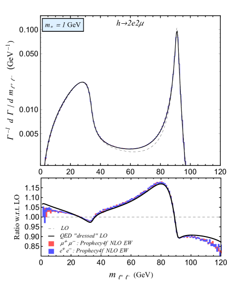
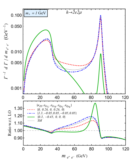
Figure 1: Left: Dilepton invariant mass spectrum in the SM for the $h\to 2e2\mu$ decay (full line: PO decomposition “dressed” with QED corrections; red and blue bands: complete NLO result from Prophecy4f). Right: Dilepton invariant mass spectrum in the presence of new physics for various benchmark scenarios (see text for details).

The complete SM NLO electroweak corrections to $h\to 4\ell$ have been computed in Bredenstein:2006rh , and the results have been implemented in the Monte Carlo event generator Prophecy4f prophecy4f . We have used Prophecy4f version 2.0 to generate $200$ millions weighted events for the recombination mass parameter $m_{*}=1$ GeV. We have used the default Prophecy4f SM inputs except for setting the Higgs boson mass to $125$ GeV. Prophecy4f adopts the dipole subtraction formalism Dittmaier:1999mb for the treatment of soft and collinear divergences, and the so-called “photon-recombination” is applied. In particular, if the invariant mass of a lepton and a photon is smaller than $m_{*}$, the photon momentum is added to the lepton momentum Bredenstein:2006rh . As a result, $m_{*}$ coincides with the collinear cut-off introduced in the previous section.

In Fig. 1 (left) we show the decay distribution as a function of the dilepton invariant mass normalized to the total decay width for $h\to 2e2\mu$ in the SM (upper plot) and the ratio between NLO and leading-order (LO) predictions (lower plot). Shown in solid black is our improved prediction obtained by convoluting the leading order distribution, shown in dashed black, with the radiator function as described in the previous section. The PO have been fixed to their SM tree-level reference values ($\kappa_{ZZ}=1$, $\epsilon_{i}=0$ Gonzalez-Alonso:2014eva ). The Prophecy4f predictions within MC uncertainty are shown with red and blue bands for $\mu^{+}\mu^{-}$ and $e^{+}e^{-}$ invariant mass spectra, respectively.

We list here a series of conclusions that can be derived from this numerical comparison.

• The spectrum obtained with the PO decomposition of the amplitude, “dressed” with leading QED corrections, provides an excellent approximation (within 1% accuracy) to the spectrum obtained with full NLO EW corrections.

• The effect of the leading QED corrections can be large, exceeding $10\%$ in specific regions of the phase space. It therefore must be included, in view of a precise data-theory comparison, also when fitting beyond-the-SM parameters.

• The PO “dressed” spectrum is obtained setting $\epsilon_{i}=0$ (i.e. to their LO SM values). The good agreement with the complete NLO calculation confirms that the $O(\alpha/\pi)$ redefinition of the $\epsilon_{i}$ is a small effect, with no observable consequences for the $h\to 2e2\mu$ dilepton invariant mass spectrum.

4 Implications for New Physics

As shown in Fig. 1 (left), radiative corrections can be sizable and must be included also when going beyond the SM. Having demonstrated the validity of our QED improved predictions to describe such effects, we are in position to apply the method in the presence of an arbitrary new physics contribution to $h\to 2e2\mu$ decay as parameterised by generic PO Gonzalez-Alonso:2014eva . As an illustrative example, we consider the impact of the leading QED corrections for non-standard values of $\kappa_{ZZ}$, $\epsilon_{Ze_{L}}$, $\epsilon_{Ze_{R}}$, $\epsilon_{Z\mu_{L}}$, and $\epsilon_{Z\mu_{R}}$.

To draw some general conclusions we analyse three benchmark points, chosen such that the deviations of the total $h\to 2e2\mu$ decay rate from the SM prediction are always small, but the impact on the spectrum are quite different. The results of the inclusion of QED corrections are shown in Fig. 1 (right). As in the left panels, we plot the dilepton invariant mass distribution normalized to the total rate (upper plot) and the ratio between NLO and LO (lower plot).

The definition of the benchmarks, and the consequences following from the analysis of radiative corrections, are listed below.

• Benchmark I [$\kappa_{ZZ}=1.3$, $\epsilon_{Ze_{L}}=\epsilon_{Z\mu_{L}}=-0.05$ , $\epsilon_{Ze_{R}}=\epsilon_{Z\mu_{R}}=0.05$ (dot-dashed blue)].
  Here the deviation from the SM point in the Higgs PO parameter space is small: this benchmark point is compatible with naive power counting in the linear EFT expansion. As a consequence, small deformations in the spectrum are obtained (upper panel) and the relative QED corrections are SM-like (lower panel). In this regime, the leading QED corrections can be directly extracted from the SM result (via an appropriate NLO/LO re-weighting).

• Benchmark II [$\kappa_{ZZ}=0$, $\epsilon_{Ze_{L}}=\epsilon_{Z\mu_{L}}=0.26$, $\epsilon_{Ze_{R}}=\epsilon_{Z\mu_{R}}=0$ (dotted red)].
  Here the deviation from the SM point is sizable, beyond the naive power counting within a generic EFT (both linear and non-linear). However, the PO configuration is such that the deviations from the SM in the spectrum are small. This implies that the relative impact of QED corrections is still SM-like.

• Benchmark III [$\kappa_{ZZ}=0.3$, $\epsilon_{Ze_{L}}=-0.45$ and $\epsilon_{Z\mu_{L}}=\epsilon_{Ze_{R}}=\epsilon_{Z\mu_{R}}=0$ (solid green)].
  In this example we observe a sizable distortion of the dilepton shape (upper panel). As a consequence, the relative impact of the QED corrections is quite different from the SM case (a description of radiative corrections by NLO/LO re-weighting of the SM result would not provide a good approximation).

5 Conclusions

The dominant electroweak corrections to $h\to 4\ell$ decays are due to the universal soft and collinear photon emission. As shown in Fig. 1, these can lead to distortions of the dilepton invariant spectrum of $O(10\%)$ is specific regions of the phase space. These effects are of the same order as the expected modifications from the SM under the assumption of underlining linear EFT Gonzalez-Alonso:2015bha . It is then mandatory to properly incorporate these corrections in a consistent way both within and beyond the SM.

As we have shown in this paper, this can be achieved in general terms within the framework of the Higgs PO. In particular we have shown that: (i) the QED corrected predictions for the $h\to 2e2\mu$ dilepton invariant mass spectra, with PO fixed to their SM LO values, are in agreement with the full NLO electroweak SM predictions within $1\%$ accuracy; (ii) the QED corrections in the presence of NP can be sizable and significantly different from the SM case.

- (1) M. Gonzalez-Alonso, A. Greljo, G. Isidori and D. Marzocca, Eur. Phys. J. C 75, no. 3, 128 (2015) [arXiv:1412.6038].
- (2) D. R. Yennie, S. C. Frautschi and H. Suura, Annals Phys. 13, 379 (1961).
- (3) S. Weinberg, Phys. Rev. 140 (1965) B516.
- (4) N. Davidson, T. Przedzinski and Z. Was, [arXiv:1011.0937].
- (5) T. Sjostrand, S. Mrenna and P. Z. Skands, Comput. Phys. Commun. 178, 852 (2008) [arXiv:0710.3820].
- (6) T. Gleisberg et al., JHEP 0902, 007 (2009) [arXiv:0811.4622].
- (7) G. Isidori, Eur. Phys. J. C 53 (2008) 567 [arXiv:0709.2439].
- (8) C. Hartmann and M. Trott, arXiv:1505.02646.
- (9) M. Ghezzi, R. Gomez-Ambrosio, G. Passarino and S. Uccirati, 1505.03706.
- (10) A. Bredenstein, A. Denner, S. Dittmaier and M. M. Weber, Phys. Rev. D 74, 013004 (2006) [hep-ph/0604011].
- (11) http://omnibus.uni-freiburg.de/sd565/programs/prophecy4f/prophecy4f.html
- (12) S. Dittmaier, Nucl. Phys. B 565, 69 (2000) [hep-ph/9904440].
- (13) M. Gonzalez-Alonso, A. Greljo, G. Isidori and D. Marzocca, arXiv:1504.04018, to appear in EPJC.