IPPP/15/41 — DCPT/15/82 — MCNET-15-17 — Cavendish-HEP-15/04 — ZU-TH 18/15

Heavy charged Higgs boson production at the LHC

Céline Degrande^[a], Maria Ubiali^[b], Marius Wiesemann^[c] and Marco Zaro^[d,e]

^[a] Institute for Particle Physics Phenomenology, Department of Physics,
Durham University, Durham DH1 3LE, United Kingdom
^[b] Cavendish Laboratory, HEP group,
University of Cambridge, J.J. Thomson Avenue, Cambridge CB3 0HE, United Kingdom
^[c] Physik-Institut, Universität Zürich,
Winterthurerstr. 190, 8057 Zurich, Switzerland
^[d] Sorbonne Universités, UPMC Univ. Paris 06,
UMR 7589, LPTHE, F-75005, Paris, France
^[e] CNRS, UMR 7589, LPTHE, F-75005, Paris, France

Abstract

In this paper we study the production of a heavy charged Higgs boson in association with heavy quarks at the LHC, in a type-II two-Higgs-doublet model. We present for the first time fully-differential results obtained in the four-flavour scheme at NLO accuracy, both at fixed order and including the matching with parton showers. Relevant differential distributions are studied for two values of the charged boson mass and a thorough comparison is performed between predictions obtained in the four- and five-flavour schemes. We show that the agreement between the two schemes is improved by NLO(+PS) corrections for observables inclusive in the degrees of freedom of bottom quarks. We argue that the four-flavour scheme leads to more reliable predictions, thanks to its accurate description of the bottom-quark kinematics and its small dependence on the Monte Carlos, which in turn is rather large in the five-flavour scheme. A detailed set of recommendations for the simulation of this process in experimental analyses at the LHC is provided.

1 Introduction

Charged Higgs bosons appear in several extensions of the scalar sector of the Standard Model (SM). In particular, as the SM does not include any elementary charged scalar particle, the observation of a charged Higgs boson would necessarily point to the presence of new physics.

In this paper we focus on one of the simplest extensions of the SM featuring a charged scalar, namely the two-Higgs-doublet model (2HDM). Within this class of models, the existence of five physical Higgs bosons, including two (mass-degenerate) charged particles $H^{\pm}$, is foreseen. Imposing flavour conservation, there are four different ways to couple the SM fermions to the two Higgs doublets. Each of these four ways of assigning the couplings gives rise to a different phenomenology for the charged Higgs boson. Here we consider the so-called type-II 2HDM, in which one doublet couples to up-type quarks and the other to the down-type quarks and the charged leptons. The Minimal Supersymmetric Standard Model (MSSM), up to SUSY corrections, belongs to the type-II 2HDM category.

Light charged Higgs scenarios are classified by Higgs boson masses smaller than the mass of the top quark (typically $m_{H^{\pm}}\lesssim 160\,\textrm{GeV}$), where the top decay to a charged scalar and a bottom quark is allowed. One refers to heavy charged Higgs bosons, on the other hand, for masses larger than the top-quark mass (typically $m_{H^{\pm}}\gtrsim 180\,\textrm{GeV}$). In this case, the dominant $H^{\pm}$ production channel at the Large Hadron Collider (LHC) is the associated production with a top quark/antiquark and a (possibly low transverse momentum) bottom antiquark/quark. In the intermediate-mass range ($160\lesssim m_{H^{\pm}}\lesssim 180\,\textrm{GeV}$) width effects become important and the full amplitude for $pp\to H^{\pm}W^{\mp}b\bar{b}$ (including non-resonant contributions) must be taken into account for a proper description. The intermediate-mass range has not been studied so far at the LHC Run I.

Searches at LEP have set a limit $m_{H^{\pm}}>80\,\textrm{GeV}$ on the mass of a charged Higgs boson for a type-II 2HDM [1]. The Tevatron limits [2, 3] have been superseded by results of the LHC experiments. Recent ATLAS results [4] for a type-II 2HDM based on 19.5 fb^-1 of $pp$ collisions at 8 TeV exclude $\textrm{BR}(t\rightarrow bH^{+})\cdot\textrm{BR}(H^{+}\rightarrow\tau^{+}\nu_{\tau})$ larger than $(0.23-1.3)\%$ in the low-mass region ($80\,\textrm{GeV}<m_{H^{\pm}}<160\,\textrm{GeV}$). For the first time limits on $tH^{+}$ production times $\textrm{BR}(H^{+}\rightarrow\tau^{+}\nu_{\tau})$ are provided for $180\,\textrm{GeV}<m_{H^{\pm}}<1000\,\textrm{GeV}$. Rates above 0.76 pb at low masses and 4.5 fb at large masses are excluded. A preliminary note by CMS [5], based on the analysis of 19.7 fb^-1 of $pp$ collisions at 8 TeV in the same search channel, sets an upper limit on $\textrm{BR}(t\rightarrow bH^{+})\cdot\textrm{BR}(H^{+}\rightarrow\tau^{+}\nu_{\tau})$ between $(0.16-1.2)\%$ in the low-mass region ($80\,\textrm{GeV}<m_{H^{\pm}}<160\,\textrm{GeV}$). This limit supersedes the one published in Ref. [6]. In the high-mass region (180 GeV $<m_{H^{\pm}}<$ 600 GeV), limits on $tH^{+}$ production times $\textrm{BR}(H^{+}\rightarrow\tau^{+}\nu_{\tau})$ are set between 0.38 pb and 26 fb. Finally, CMS has also published a preliminary note [7] on a direct search for a heavy charged Higgs which decays in both the $H^{+}\to t\bar{b}$ and the $H^{+}\to\tau^{+}\nu_{\tau}$ channels.

In this work, we consider heavy charged Higgs boson production at hadron colliders and leave the intermediate-mass range to future studies [8]. In particular, we focus only on the production of a negatively charged scalar since the results are identical for a positively charged scalar. As for any process involving bottom quarks at the matrix-element level, two viable schemes exist to compute the production cross section of a heavy charged Higgs boson. These are usually dubbed as four- and five-flavour schemes. In the four-flavour scheme (4FS) the bottom quark mass is considered as a hard scale of the process. Therefore, bottom quarks do not contribute to the proton wavefunction and can only be generated as massive final states at the level of the short-distance cross section, entailing that $b$-tagged observables receive contributions starting at leading order (LO). In practice, the theory which is used in such a calculation is an effective theory with four light quarks, where the massive bottom quark is decoupled and enters neither the renormalisation group equation for the running of the strong coupling constant nor the evolution of the parton distribution functions (PDFs). The LO partonic processes in the case at hand are

$$gg\rightarrow H^{-}\bar{b}t\quad\text{and}\quad q\bar{q}\rightarrow H^{-}\bar{b}t\,.$$ (1)

Next-to-leading order (NLO) calculations for the total cross sections in this scheme have been presented in Refs. [9, 10].

Conversely, in five-flavour scheme (5FS), the bottom quark mass is considered to be much smaller than the hard scales involved in the process. The simplest definition of the 5FS—that suits particularly well perturbative computations—is to strictly set $m_{b}=0$ in the short-distance cross section. Consequently, bottom quarks are treated on the same footing as all other massless partons. The only difference is the presence of a threshold in the bottom-quark PDF and the initial condition of the bottom quark evolution being of perturbative nature. The use of $b$-PDFs comes along with the approximation that, at leading order, the massless $b$ quark has a small transverse momentum. In this scheme, the leading logarithms associated to the initial state collinear splitting are resummed to all orders in perturbation theory by the Dokshitzer-Gribov-Lipatov-Altarelli-Parisi (DGLAP) evolution of the bottom densities. The LO partonic process is given by

$$gb\rightarrow H^{-}t\,.$$ (2)

Next-to-leading order predictions for heavy charged Higgs boson production in the 5FS, possibly including the matching to parton-shower Monte Carlos, were studied in Refs. [11, 12, 13, 14, 15, 16, 17]. Electroweak corrections [18, 19] and soft gluon resummation effects [20, 15, 21] have also been included in recent works.

The leading-order diagrams in the 4FS and 5FS are displayed in Fig. 1.

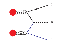
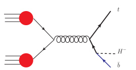
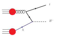
Figure 1: Leading-order diagrams for heavy charged Higgs and top associated production, in the 4FS (left and centre) and 5FS (right).

The comparison between the two schemes at the level of total cross section has been performed by several groups, see e.g. Ref. [10] and references therein. In a more recent study [22] a thorough combination of all sources of theoretical uncertainties is performed, state-of-the-art PDF sets are used, the new scale-setting procedure proposed in Refs. [23, 24] is adopted and a Santander-matched prediction [25] of the four- and five-flavour scheme computations is provided. Furthermore, a comparison of five- and six-flavour schemes, assessing the effect of the inclusion of top PDFs, has been recently performed at the level of total cross sections [26]. In summary, these studies establish a generally good agreement of total cross section predictions in different flavour schemes, once a judicious scale choice is made.

Studies at differential level of heavy charged Higgs production in four- and five-flavour schemes are very limited, if not absent. NLO plus Parton Shower (PS) accurate predictions are available only in the 5FS for both MC@NLO [16] and POWHEG [17], and their comparison to 4FS results at the level of differential distributions has never been performed to date. Such a differential study is certainly more involved than the inclusive one, mainly for two reasons. First of all, there is a very large number of possibly relevant observables at the differential level. Second, differences between the two schemes are generally larger than in the inclusive case. As a consequence, an even more careful assessment of the related uncertainties is necessary for distributions. Indeed, observables inclusive in the degrees of freedom of the bottom quarks, such as total cross sections, turn out to be quite similar in four- and five-flavour schemes. On the one hand power-suppressed terms are small for this class of observables. On the other hand collinear logarithms are phase-space suppressed [23] and therefore moderate, unless a very heavy charged Higgs is produced.

As far as exclusive observables are concerned, it is vital to investigate 4FS and 5FS predictions and assess their differences on a case-by-case basis in an unbiased manner, which is one of the main goals of this paper. The generic rationale is the following: if power-suppressed terms are relevant, the 4FS provides a more reliable prediction, while if collinear logarithms are large, the reorganisation of the perturbative series in the 5FS improves the stability of the perturbative expansion.

The comparison of the two schemes is further complicated by the fact that observables related to light and $b$-flavoured jets are associated with different perturbative orders: while in charged Higgs production one final-state $b$ quark (not accounting for top decays) is already present at LO in the 4FS, a final-state $b$ quark enters the 5FS computation only at NLO. Furthermore, tagging $b$ quarks in a 5FS fixed-order computation necessarily leads to unphysical results, since they can be considered only as part of jets to retain infra-red cancellations. This issue clearly does not affect the 4FS, in which observables related to the $b$ quarks are regulated by the $b$ mass. Nevertheless, when considering $b$ quarks at very large transverse momenta, $b$-jet observables have to be preferred anyway, otherwise large logarithms $\log(p_{T}/m_{b})$ would spoil the perturbative convergence.

Matching to parton showers improves most notably the 5FS predictions, since the parton backward evolution of the initial-state bottom quarks turns them into massive final states and further generates $b$-flavoured hadrons which renders $b$-tagging realistic. One should bear in mind, however, that the details and the actual implementation of such backward evolution are highly non-trivial—being based on DGLAP evolution equations, which are only LL accurate—and therefore turn out to be widely Monte Carlo dependent (see Sect. 3.3 of Ref. [27], and Sect. 3.3 below). Moreover, the necessity of reshuffling the massless into massive bottom quarks may have significant effects on the kinematics of final-state $B$ hadrons. In the 4FS, the shower primarily improves the description of Sudakov-suppressed small-$p_{T}$ radiation, by resumming leading collinear logarithms to all orders. In both schemes the PS introduces additional power-suppressed terms in the soft region.

In this paper, we present for the first time NLO+PS accurate 4FS predictions and thoroughly compare them to the 5FS ones. Our primary aim is to acquire a detailed understanding and assess which scheme is better suited for the simulation of the charged Higgs production signal, whose search represents a central part of the physics program in (and beyond) Run II at the LHC. As will be shown, our analysis confirms and extends the conclusions that have been drawn in previous studies of differential distributions in the four- and five-flavour schemes, in the context of Higgs production in association with bottom quarks [28] and Higgs and single-top associated production [29]. Similar analyses were performed for single top production [30, 31]. Moreover, given that the mass of the charged Higgs boson is still allowed to take almost arbitrarily large values, this process is perfectly suited for a case-study of different flavour schemes in QCD in a broad range of scales.

The paper is structured as follows: in Sect. 2 an outline of the calculation is given and details of the implementation of the 4FS calculation at NLO+PS accuracy are provided. Results are displayed in Sect. 3, in which the features of the 4FS calculation are described, including the size of the interference term that appears in this scheme, and the 4FS and 5FS distributions are compared. We conclude in Sect. 4 with our final recommendations for experimental analyses.

2 Outline of the calculation

Our computation takes advantage of a full chain of automatic tools developed to study the phenomenology of new physics models at NLO QCD accuracy in the MadGraph5_aMC@NLO [32] framework.

2.1 Framework

Besides the usual tree-level Feynman rules, some extra ingredients have to be provided to the matrix-element generator in order to obtain the code for the simulation of a new physics process at NLO. These extra ingredients are the Ultra-Violet (UV) renormalisation counter-terms and a sub-class of the rational terms that enter the reduction of the virtual matrix elements, the so-called $R_{2}$ terms [33]. UV and $R_{2}$ counter-terms can be computed starting from the model Lagrangian for any renormalisable theory via the NLOCT package [34], based on FeynRules [35] and FeynArts [36]. The tree-level and NLO Feynman rules are exported in the Universal Feynrules Output (UFO) [37] format, as a Python module which can be loaded by matrix-element generators, such as MadGraph5_aMC@NLO. Finally, the UFO information is translated into helicity routines [38] by ALOHA [39].

We remind the reader that MadGraph5_aMC@NLO is a meta-code that automatically generates the code for simulating any process at NLO(+PS) accuracy. MadGraph5_aMC@NLO adopts the FKS method [40, 41] for the subtraction of the singularities of the real-emission matrix elements, as automated in the MadFKS module [42]; virtual matrix elements are computed via the MadLoop module [43], which relies on the OPP [44] and Tensor Integral Reduction (TIR) [45, 46] methods, as implemented in CutTools [47] and IREGI [48], supplemented by an in-house implementation of the OpenLoops procedure [49]; finally, the generation of hard events and their matching to parton-shower simulations is performed à la MC@NLO [50]. The matching to Herwig6 [51], Pythia6 [52] (ordered in virtuality or in transverse momentum, the latter only for processes with no light partons in the final state), Herwig++ [53] and Pythia8 [54] is available. As a consequence, the only inputs needed are the implementation of the model in FeynRules and the inclusion of the running of the bottom quark mass, which follows from our renormalisation-scheme choice. More details are given in the next section. Both the 4FS and the 5FS computations have been performed in the framework specified above, with the additional advantage of ensuring the consistency of all settings and input parameters.

To guarantee the validity of our analysis, we have performed a detailed comparison of the inclusive cross sections obtained with MadGraph5_aMC@NLO against previous results published in literature. The calculation in the 4FS has been compared to the private code of Ref. [10] at the level of total rates, and a good agreement within the numerical uncertainty of the reference code has been found. Furthermore, with the bottom quark Yukawa renormalised on-shell and with its mass set the value of the top pole mass, we reproduce the $t\bar{t}H$ total cross section in the SM at the few per-mille level.

2.2 Implementation

We have used the implementation of the generic 2HDM in FeynRules detailed in Ref. [34]. This model has been converted into a type-II 2HDM by adding $\beta$ as an external parameter and by restricting the Yukawa couplings accordingly. If top and bottom quarks are assumed to be the only massive fermions, the only non-zero entries of the Yukawa coupling matrices to the doublet without vacuum expectation value in the Higgs basis for the type-II 2HDM are given by

$$G^{u}_{3,3}=-\sqrt{2}\,\frac{m_{t}^{y}}{v}\,\cot\beta\quad\text{and}\quad G^{d}_{3,3}=\sqrt{2}\,\frac{m_{b}^{y}}{v}\,\tan\beta,$$ (3)

where $m_{t/b}^{y}$ are the Yukawa masses of the top and bottom quark. The parameter $\tan\beta=v_{2}/v_{1}$ is the ratio of the vacuum expectation values $v_{1}$ and $v_{2}$ of the two Higgs doublets, such that $v^{2}\equiv v_{1}^{2}+v_{2}^{2}=(\sqrt{2}G_{F})^{-1}$ is the SM Higgs vacuum expectation value, where $G_{F}$ is the Fermi constant. With those restrictions, the $H^{-}t\bar{b}$ vertex is given by

$$V_{t\bar{b}H^{-}}=-i\left(y_{t}P_{R}\,\frac{1}{\tan\beta}+y_{b}P_{L}\tan\beta\right),$$ (4)

where $P_{R/L}=(1\pm\gamma_{5})/2$ are the chirality projectors and $y_{t/b}\equiv\sqrt{2}\frac{m_{t/b}^{y}}{v}$ are the corresponding SM Yukawa couplings. We strictly separate the Yukawa masses that are used in the computation of the couplings between the fermions and the scalars from the kinematic masses that are used everywhere else and set to the on-shell mass. This distinction allows us to keep a non-vanishing bottom Yukawa in the five-flavour scheme as the leading term in the small $m_{b}$ expansion [13, 14]. Furthermore, it allows us to choose different renormalisation schemes for the bottom quark mass in the matrix element and in the Yukawa coupling.

The model $R_{2}$ and UV vertices required for NLO computations in MadGraph5_aMC@NLO have been computed using NLOCT [34]. The masses and the wave functions are renormalised in the on-shell scheme to avoid the computation of loops on external legs. The strong coupling constant is renormalised in the $\overline{\text{MS}}$ scheme with the contribution of massive quarks subtracted from the gluon self-energy at zero-momentum transfer. Therefore, only the massless modes affect the running of $\alpha_{s}$. The renormalisation of the masses in principle fixes the renormalisation of the top and bottom Yukawa since

$$\delta y_{t/b}=\sqrt{2}\frac{\delta m_{t/b}}{v},$$ (5)

with

$$\delta m_{t/b}=-\frac{g_{s}^{2}}{12\pi^{2}}m_{t/b}\left(\frac{3}{\bar{\epsilon}}+4-6\log\frac{m_{t/b}}{\mu_{R}}\right)\,$$ (6)

in the on-shell scheme. This is the default renormalisation used in NLOCT and it would ensure that nothing but the strong coupling constant depends on the renormalisation scale. The top mass and Yukawa are always renormalised in this way throughout this paper. Therefore its Yukawa mass is set equal to the pole mass. On the contrary, the bottom quark Yukawa has been renormalised in the $\overline{\text{MS}}$ scheme, i. e.

$$\delta y_{b}=-\frac{\sqrt{2}}{v}\frac{g_{s}^{2}m_{b}^{y}}{4\pi^{2}\bar{\epsilon}}\,.$$ (7)

This scheme choice has the advantage of resumming potentially large logarithms $\log(\mu_{R}/m_{b})$ (with $\mu_{R}\sim m_{H^{\pm}}$) to all orders. The bottom Yukawa mass is set to the value of the running $\overline{\text{MS}}$ mass at the renormalisation scale. Besides the modifications at the level of the UFO model, also the code written by MadGraph5_aMC@NLO had to be changed in order to account for the additional scale dependence introduced by the $b$-quark Yukawa, in particular for what concerns the on-the-fly evaluation of scale uncertainties obtained via reweighting [56]. This has been done in an analogous way as for bottom-associated Higgs production [28], by splitting the cross section in parts that factorise different powers of $y_{b}$, i. e. $y_{b}^{2}$, $y_{b}\,y_{t}$ and $y_{t}^{2}$.

3 Results

In this section, we present four-flavour scheme predictions of charged Higgs boson production at NLO matched to parton showers. This calculation has never been performed before in the literature. Several differential distributions that are reconstructed from the final state particles in $tH^{-}\bar{b}$ production are studied. We investigate the role of the shower scale in this process, discuss the impact of the $y_{b}y_{t}$ interference term and compare our reference predictions at (N)LO+PS to the f(N)LO results. For matched predictions, both Herwig++ and Pythia8 are employed. We conclude this chapter with a comprehensive comparison of 4FS and 5FS distributions, in which the effects of higher order corrections, the impact of the choice of the shower scale and the dependence of each scheme on the different Monte Carlos are analysed.

3.1 Settings

We present results for charged Higgs boson production at the LHC Run II ($\sqrt{S}_{\rm had}=13\,\textrm{TeV}$) by considering two scenarios: a lighter ($m_{H^{\pm}}=200\,\textrm{GeV}$) and a heavier ($m_{H^{\pm}}=600\,\textrm{GeV}$) charged Higgs boson. For simplicity, we set $\tan\beta=8$ throughout this paper. At this value, $y_{b}^{2}$ and $y_{t}^{2}$ terms are of similar size and the relative contribution of the $y_{b}y_{t}$ term to the total cross section is close to its maximum. Results for any other value of $\tan\beta$ can be obtained by a trivial overall rescaling of the individual contributions according to their Yukawa couplings ($y_{b}$ by $\tan\beta$, $y_{t}$ by $1/\tan\beta$). Therefore, we preserve the generality of our results by studying the $y_{b}^{2}$, $y_{t}^{2}$ and $y_{b}y_{t}$ contributions separately.

We show results obtained with the NNPDF2.3 set [57] at NLO and the NNPDF3.0 [58] set at LO. To obtain consistent predictions, parton distribution functions (PDFs) computed in the proper flavour number scheme are used: we interface our NLO (LO) calculation with the NNPDF2.3 (NNPDF3.0) with $n_{f}=4$ and $n_{f}=5$ active flavours for the 4FS and 5FS respectively. The mismatch between the PDF sets used in the LO and NLO computations is due to the absence of a public set of non-QED LO PDFs in the NNPDF2.3 family. This does not affect the accuracy of our results, given that the LO PDF sets exhibit a theoretical uncertainty which is larger than the difference between the two NNPDF families. The strong coupling constant is consistent with $\alpha_{s}(M_{Z})=0.118$ for the 5FS NLO parton densities and $\alpha_{s}(M_{Z})=0.1226$ for the 4FS NLO ones.

The heavy quark pole masses are set to

$$m_{b}^{\rm pole}=4.75\,\textrm{GeV}\;\textrm{(relevant only to the 4FS)},\qquad m_{t}^{\rm pole}=172.5\,\textrm{GeV}.$$ (8)

At one loop, the value of the bottom pole mass translates into a $\overline{\text{MS}}$ mass

$$\bar{m}_{b}(\bar{m}_{b})=4.3377\,\textrm{GeV}.$$ (9)

Finally, our central renormalisation and factorisation scales $\mu_{R},\mu_{F}$ are set to

$$\mu_{R,F}=H_{T}/3\equiv\frac{1}{3}\sum_{i}\sqrt{m(i)^{2}+p_{T}(i)^{2}},$$ (10)

where the index $i$ runs over all final state particles (the top quark, the charged Higgs boson and possibly the extra $b$ quark and/or light parton) of the hard process. For vanishing transverse momenta of the external particles, our scale choice corresponds to the factorisation scale set in the 4FS calculation of Refs. [22, 10]. In the following, scale uncertainties are obtained by varying $\mu_{F}$ and $\mu_{R}$ independently by a factor of two around their central values, given in Eq. (10). We have checked that, particularly for our reference 4FS NLO+PS prediction, the dependence of the distributions on the shower scale $\mu_{\text{sh}}$, when varied by a factor in the range $[1/\sqrt{2},\sqrt{2}]$, is rather mild and significantly smaller than uncertainties associated with the renormalisation and factorisation scales; we therefore refrain from including uncertainties associated with $\mu_{\text{sh}}$ in what follows. Furthermore, we will not discuss any PDF systematics.

Jets are reconstructed via the anti-$k_{T}$ algorithm [59], as implemented in FastJet [60, 61], with a distance parameter $\Delta R=0.4$ and subject to the conditions

$$p_{T}(j)\geq 25\,\textrm{GeV},\qquad|\eta(j)|\leq 2.5.$$ (11)

For fixed-order computations jets are clustered from partonic final states, while in simulations matched to parton showers jets are made up of hadrons; $b$ jets are defined to contain at least one $b$ quark (at fixed order) or $B$ hadron (in matched simulations).

In our simulations we keep the charged Higgs boson stable, while we decay the top quark leptonically (although the leptons from the decay will not affect any observable we consider) in order to keep as much control as possible on the origin of QCD radiation. The task to decay the top quark is performed by the parton shower for (N)LO+PS runs, while at fixed order we simulate the decay $t\to bW$ in an isotropic way (in the $t$ rest frame) at the analysis level. No simulation of the underlying event is performed by the parton shower.

Let us conclude this section by addressing one further point, which is crucial when processes with final-state $b$ quarks are matched to parton showers: the choice of the shower starting scale $\mu_{\text{sh}}$. Such processes are known to prefer much lower values of the renormalisation and factorisation scales than the one naively identified as the hard scale of the process ($\hat{s}$). In fact, the shower starting scale and the factorisation scale emerge both from the same concept, namely the separation of soft and hard physics. Furthermore, it has been argued in Ref. [28] for the associated production of a neutral Higgs boson with bottom quarks that the shower starting scale (limiting the hardest emission that the shower can generate) should be set at similar values, i. e. well below $\hat{s}$. Following the arguments made in Ref. [28], we check their validity in the case of charged Higgs boson production. We shall stress at this point that the following discussion applies both to our reference scenarios with $m_{H^{-}}=200\,\textrm{GeV}$ and $m_{H^{-}}=600\,\textrm{GeV}$, although we refrain from showing explicit results for the latter.

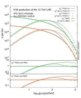
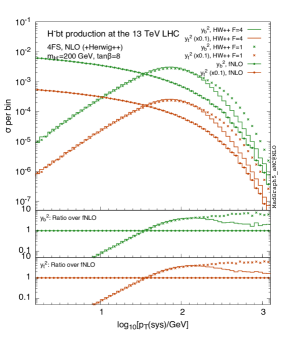
Figure 2: Transverse momentum of the $H^{-}\bar{b}t$ system for $m_{H^{-}}=200\,\textrm{GeV}{}$ in the 4FS at fNLO (green dotted-solid for the $y_{b}^{2}$ term, orange dotted-solid for the $y_{t}^{2}$ term), and at NLO+PS with $F$= 1 (green dots for the $y_{b}^{2}$ term, orange dots for the $y_{t}^{2}$ term) and $F$= 4 (green solid for the $y_{b}^{2}$ term, orange solid for the $y_{t}^{2}$ term). We show predictions matched with Pythia8 (left) and Herwig++ (right). The insets show the ratio of the curves in the main frame over the fNLO prediction, for both the $y_{b}^{2}$ and the $y_{t}^{2}$ terms.

MadGraph5_aMC@NLO assigns a dynamical shower scale chosen from a distribution in the range

$$\frac{0.1}{F}\hat{s}\leq\mu_{\text{sh}}\leq\frac{1}{F}\hat{s},$$ (12)

where $F$ is a parameter that drives the bounds of the distribution, and whose default value is $F=1$. With such a default setting the effective value of $\mu_{\text{sh}}$, namely the maximum of the $\mu_{\text{sh}}$ distribution (which for simplicity we will refer to as just $\mu_{\text{sh}}$ in the following), is indeed much larger than $\mu_{F,R}$. Furthermore, considering the transverse momentum distribution of the Born-level “system” ($p_{T}(\textrm{sys})$), which is maximally sensitive to the interplay between the fixed-order prediction and the shower, the NLO+PS distribution (in particular in the 4FS) does not match the fixed-order NLO (fNLO) one at large $p_{T}$ for $F=1$. This can be deduced from Fig. 2, when comparing the crosses (NLO+PS for $F=1$) to the solid curves overlayed with points (fNLO). On the contrary, we observe a clearly improved high-$p_{T}$ matching of the NLO+PS results to the fixed-order ones by choosing a reduced shower scale corresponding to $F=4$ (solid curves). Indeed, such a choice brings $\mu_{\text{sh}}$ much closer to the value of the renormalisation and factorisation scales. We have also checked that the agreement among Pythia8 and Herwig++ improves (although often only marginally) when differential observables in the 4FS are computed with $F=4$.

In conclusion, although for this process we do not reproduce all results of Ref. [28] with the same significance, we still find sufficient evidence that $F=4$ is favourable in many respects and make it our default choice. In Sect. 3.3, we shall further study the impact of this choice when comparing the 4FS and 5FS results: by setting $F=4$ an improved agreement between the two schemes at the level of shapes is observed.

3.2 Four-flavour scheme results

We now turn to our phenomenological results for charged Higgs boson production. Let us first consider state-of-the-art 4FS predictions, which, as will be shown, constitute the most reliable differential results for observables exclusive in the degrees of freedom of final-state bottom quarks. We split this section into two parts: in Sect. 3.2.1 we limit our study to the dominant $y_{b}^{2}$ and $y_{t}^{2}$ contributions, while the $y_{b}\,y_{t}$ contribution is considered in Sect. 3.2.2.

3.2.1 $y_{b}^{2}$ and $y_{t}^{2}$ contributions at NLO+PS

$\sigma(m_{H^{-}}=200\,\textrm{GeV})$ [fb]		NLO		LO
		$y_{b}^{2}$	$y_{t}^{2}$	$y_{b}^{2}$	$y_{t}^{2}$
Inclusive		$50.40^{+17.8\%}_{-18.6\%}$	$42.43^{+12.4\%}_{-13.1\%}$	$42.12^{+52.2\%}_{-31.9\%}$	$28.68^{+36.3\%}_{-24.7\%}$
$\geq 1j_{b}$	F.O.	$45.47^{+17.5\%}_{-18.4\%}$	$38.31^{+12.2\%}_{-13.0\%}$	$38.26^{+51.9\%}_{-31.8\%}$	$26.09^{+36.1\%}_{-24.6\%}$
	Pythia8	$43.44^{+17.4\%}_{-18.4\%}$	$36.67^{+12.0\%}_{-13.0\%}$	$36.81^{+52.0\%}_{-31.8\%}$	$25.09^{+36.1\%}_{-24.7\%}$
	Herwig++	$42.64$	$36.04$	$36.08$	$24.61$
$\geq 2j_{b}$	F.O.	$11.55^{+10.9\%}_{-15.4\%}$	$9.76^{+6.5\%}_{-10.0\%}$	$11.22^{+50.4\%}_{-31.2\%}$	$7.79^{+35.0\%}_{-24.1\%}$
	Pythia8	$12.55^{+15.3\%}_{-17.4\%}$	$10.67^{+10.4\%}_{-12.1\%}$	$11.73^{+51.2\%}_{-31.5\%}$	$8.12^{+35.6\%}_{-24.4\%}$
	Herwig++	$11.03$	$9.33$	$10.09$	$7.00$

$\sigma(m_{H^{-}}=600\,\textrm{GeV})$ [fb]		NLO		LO
		$y_{b}^{2}$	$y_{t}^{2}$	$y_{b}^{2}$	$y_{t}^{2}$
Inclusive		$2.400^{+20.3\%}_{-20.1\%}$	$2.117^{+13.1\%}_{-14.2\%}$	$1.794^{+54.9\%}_{-33.0\%}$	$1.339^{+40.1\%}_{-26.5\%}$
$\geq 1j_{b}$	F.O.	$2.187^{+19.9\%}_{-19.9\%}$	$1.925^{+12.6\%}_{-14.0\%}$	$1.649^{+54.7\%}_{-32.9\%}$	$1.232^{+39.9\%}_{-26.5\%}$
	Pythia8	$2.115^{+19.9\%}_{-19.9\%}$	$1.865^{+12.5\%}_{-14.0\%}$	$1.601^{+54.8\%}_{-32.9\%}$	$1.197^{+40.0\%}_{-26.5\%}$
	Herwig++	$2.077$	$1.836$	$1.570$	$1.175$
$\geq 2j_{b}$	F.O.	$0.630^{+12.6\%}_{-17.0\%}$	$0.548^{+5.9\%}_{-10.8\%}$	$0.548^{+53.8\%}_{-32.6\%}$	$0.413^{+39.2\%}_{-26.2\%}$
	Pythia8	$0.697^{+16.7\%}_{-18.6\%}$	$0.611^{+9.6\%}_{-12.6\%}$	$0.588^{+54.3\%}_{-32.8\%}$	$0.443^{+39.6\%}_{-26.3\%}$
	Herwig++	$0.602$	$0.532$	$0.498$	$0.376$

Table 1: 4FS predictions for total rates (in fb) for $\tan\beta=8$.

We begin our analysis by studying total rates for the production of charged Higgs bosons with a mass of $200\,\textrm{GeV}$ and $600\,\textrm{GeV}$ in Table 1. We consider three possibilities: the fully inclusive case, the case in which we require at least one $b$ jet, and the one in which two or more $b$ jets are tagged. All results are given at both LO and NLO accuracy. The cross sections in which one or two $b$ jets are required depend on the approximation and Monte Carlo under consideration. We thus report separately results obtained at fixed order, with Pythia8 and with Herwig++. Any quoted uncertainty is due to scale variation, evaluated as detailed in Sect. 3.1; they are indicated only at fixed order and for results matched with Pythia8, since they show little dependence on the specific Monte Carlo. Results for $y_{b}^{2}$ and $y_{t}^{2}$ terms are presented separately. Let us summarize the conclusions to be drawn from Table 1 as follows:

• The scale uncertainty of NLO predictions is substantially smaller than that of the LO ones; at NLO the scale uncertainty is larger for the $y_{b}^{2}$ than for the $y_{t}^{2}$ contribution ($\sim 15$-$20\%$ and $\sim 10$-$15\%$, respectively), due to the different renormalisation schemes used for the bottom and top Yukawa couplings.

• Because of our default choice of $\tan\beta=8$, $y_{b}^{2}$ and $y_{t}^{2}$ predictions are of similar size at NLO (only $\sim 15\%$ different); the difference is larger at LO ($\sim 30$%). As a consequence, the $K$-factors are generally different between the $y_{b}^{2}$ and $y_{t}^{2}$ terms; for $m_{H^{-}}=200\,\textrm{GeV}$, the inclusive $y_{b}^{2}$ $K$-factor is close to 1.2, while for the $y_{t}^{2}$ term the NLO corrections have a larger impact, with $K\approx 1.5$; for $m_{H^{-}}=600\,\textrm{GeV}$, NLO corrections are larger in both cases: $K\approx 1.3$ and $K\approx 1.6$ for the $y_{b}^{2}$ and $y_{t}^{2}$ terms respectively. The smaller $K$-factor for the $y_{b}^{2}$ term is a consequence of the fact that, by renormalising the bottom Yukawa in the $\overline{\text{MS}}$ scheme, the LO predictions already include a class of higher order corrections.

• Pythia8 and Herwig++ predictions for cross sections with $b$-jet requirements are consistent with each other and well within quoted uncertainties; this holds true both at the LO and at the NLO. Even the agreement with the fixed-order results is rather good overall and largely within uncertainties. Higher $b$-jet multiplicities tend to deteriorate the agreement, although only to a small extent.

• The effect of the cuts on the number of $b$ jets is quite moderate: given that there is generally a hard $b$ jet from the top quark decay, the inclusive rate is reduced by only $\sim 10\%$, when at least one $b$ jet is required. On the other hand, requiring a second $b$ jet reduces the cross section by a factor of 4-5. Scale uncertainties slightly decrease at NLO for cross sections within cuts.

We now turn to differential observables in the 4FS. We only discuss results at fixed order and matched with Pythia8. Any differences to the matched Herwig++ predictions will be explicitly mentioned below. Besides, the Monte Carlo dependence will be investigated in more detail when comparing distributions in the two flavour schemes in Sect. 3.3.

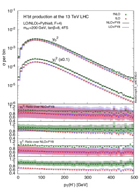
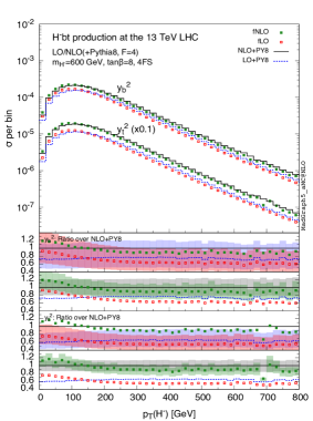
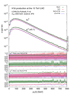
Figure 3: Transverse momentum distributions of the charged Higgs (left panels) and the top quark (right panels) for $m_{H^{-}}=200\,\textrm{GeV}$ (upper panels) and $m_{H^{-}}=600\,\textrm{GeV}$ (lower panels); predictions at fixed order (LO red empty boxes, NLO green full boxes) as well as matched to Pythia8 (LO blue dashes, NLO black solid) are shown in the main frame, for the $y_{b}^{2}$ and $y_{t}^{2}$ terms separately. The first and second (third and fourth) insets show the ratios of the curves in the main frame over the matched NLO prediction, for the $y_{b}^{2}$ ($y_{t}^{2}$) term respectively, together with the LO and NLO uncertainty bands.

The figures throughout this section are organised according to the following pattern: the main frame displays the relevant predictions in absolute size as cross section per bin for the $y_{b}^{2}$ and $y_{t}^{2}$ terms. For the sake of readability, they have been separated by reducing the $y_{t}^{2}$ curve by a factor of ten. The fixed-order results are shown using boxes, while simulations matched to parton showers are displayed as lines: filled green boxes for fNLO, open red boxes for fLO, a black solid line for NLO+PS and a blue dotted curve for LO+PS. In the first two insets we display the bin-by-bin ratio of all $y_{b}^{2}$ histograms in the main frame normalised to the corresponding NLO+PS result. The difference between the two insets are the uncertainty bands, which in the first one are displayed for the LO predictions, while in the second for the NLO ones. The third and fourth insets are identical to first two, but for the $y_{t}^{2}$ contribution.

Let us start in Fig. 3 with the transverse momentum spectrum of a $200\,\textrm{GeV}$ Higgs (top left panel) and the associated top quark (top right panel). The two plots are in fact quite similar and can be discussed simultaneously: the agreement between the fixed-order and the PS-matched simulations is close-to-excellent in all cases. Matching to the PS has only minor effects on the shape of the distributions, notable only at small transverse momenta. In other words, the resummation effects of the shower are extremely small, as can be expected from observables that are practically not affected by any large Sudakov logarithm. The NLO corrections mostly affect the normalisation and reduce theoretical uncertainties, reflecting the numbers quoted in Tab. 1. We stress here two general features regarding the relation between the $y_{b}^{2}$ and $y_{t}^{2}$ terms which shall hold true for all subsequent observables under consideration: first, the $\overline{\text{MS}}$ renormalisation makes the uncertainty associated with the $y_{b}^{2}$ curves larger, due to the variation of $\mu_{R}$ in $y_{b}\sim\bar{m}_{b}(\mu_{R})$; second, the ratio of the $y_{b}^{2}$ and $y_{t}^{2}$ contributions at NLO is generally flat. More details will be given in Sect. 3.3.

For a heavier charged Higgs boson with mass $m_{H^{-}}=600\,\textrm{GeV}$, the lower panels of Fig. 3 display a similar behaviour as in the $m_{H^{-}}=200\,\textrm{GeV}$ case. Larger effects due to the PS are visible in the Higgs $p_{T}$ spectrum at low transverse momenta.

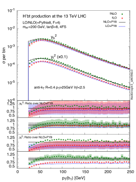
Figure 4: Same as the upper panel of Fig. 3, but for the transverse momentum of hardest (left panel) and second-hardest (right panel) $b$ jet.

We continue our presentation of the 4FS results with the transverse momentum spectra of the hardest ($p_{T}(b_{1})$) and second-hardest ($p_{T}(b_{2})$) $b$ jet in Fig. 4; see Sect. 3.1 for our jet (and $b$ jet) definition. In this case, we limit our discussion to $m_{H^{-}}=200\,\textrm{GeV}$ results, since, apart from a naturally smaller cross section, the relative behaviour of the different curves is extremely similar for a heavier charged scalar. Although the $p_{T}(b_{1})$ and $p_{T}(b_{2})$ distributions in the main frame develop a quite different behaviour in terms of their shapes, the ratios in the insets exhibit comparable features: in all cases, the tail of the spectra is driven by the order relevant to the simulation and NLO corrections slightly soften the spectra. In other words, the fixed-order results agree rather well with the corresponding Pythia8 ones in the tail. On the other hand, close to threshold ($p_{T}=25$ GeV), where resummation effects are enhanced, non-showered and showered results exhibit sizeable differences, in particular for the hardest $b$ jet.

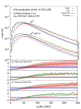
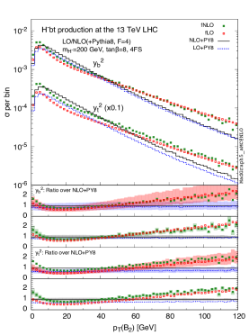
Figure 5: Same as the upper panel of Fig. 3, but for the transverse momentum of hardest (left panel) and second-hardest (right panel) $B$ hadrons.

Turning now to somewhat related observables in Fig. 5—the transverse momentum distributions of the hardest and second-hardest $B$ hadron—, one may expect rather similar features to the $b$-jet transverse momentum spectra. On the contrary, their pattern is actually very different; the salient feature being that showered results are vastly softer than the fixed-order ones and a substantial shape distortion due to the matching with parton showers is observed. In fact, even the peak of the $p_{T}(B_{1})$ distribution is moved by $\sim 25\,\textrm{GeV}$ towards the left by the shower. However, one should bear in mind that we compare bottom quarks at parton level for the f(N)LO predictions with $B$ hadrons at (N)LO+PS. The observed differences unavoidably lead to the conclusion that fragmentation effects become significant for such exclusive observables. Otherwise, the pattern of the Pythia8 results is very much reminiscent of $b$-jet spectra, displaying a slightly harder LO+PS shape than at NLO+PS. Generally speaking, the relative behaviour of the $y_{b}^{2}$ and $y_{t}^{2}$ curves is pretty much alike, including the peculiar increase of the f(N)LO cross section towards vanishing $p_{T}(B_{2})$. Again, we refrain from showing explicit results for a $m_{H^{-}}=600\,\textrm{GeV}$ charged Higgs boson, since the pattern of the various curves turns out to be very similar to the $m_{H^{-}}=200\,\textrm{GeV}$ case; the only difference to be pointed out is a slightly reduced gap between showered and fixed-order results for $m_{H^{-}}=600\,\textrm{GeV}$.

We investigated a vast number of differential observables, the majority of which follows the same pattern as illustrated in Figs. 3 and 4: the NLO corrections are rather flat and lie within the LO uncertainty bands, shower effects are moderate and become more substantial the more exclusive the observable is with respect to the bottom-quark degrees of freedom.

Figure 6: Same as the upper panel of Fig. 3, but for the invariant mass of the two hardest $B$ hadrons (left panel) and their distance in the $\eta-\phi$ plane (right panel).

Based on our findings, we do not expect larger effects for $b$-jet observables than for distributions relevant to $B$ hadrons. Therefore it is worth to consider the invariant mass $M(B_{1},B_{2})$ of and the distance $\Delta R(B_{1},B_{2})$ in the $\eta-\phi$ plane between the two hardest $B$ hadrons, which are displayed in the left and right panels of Fig. 6 respectively. The reader should keep in mind that in the fixed-order cases the two hardest $b$ quarks are used instead. Since there are no salient differences for larger Higgs masses we only discuss the $m_{H^{-}}=200\,\textrm{GeV}$ results.

Although the invariant mass is quite a different observable than the transverse momentum of the hardest $B$ hadron, our findings are actually rather similar, but less pronounced: the shower substantially affects the distributions, by causing a significant softening whose size exceeds the uncertainty bands of the fixed-order calculations. This effect reflects the loss of energy of the $b$ quarks due to their fragmentation into $B$ hadrons. These observations are to a good extend independent of the considered contribution ($y_{b}^{2}$ or $y_{t}^{2}$).

In contrast, the effect of the shower in the $\Delta R(B_{1},B_{2})$ distribution is smaller and becomes relevant only at large separations ($\Delta R\geq 4.5$). We point out that such large separations are at or beyond the coverage edge of the $b$ tracking system of LHC experiments, and that if two $b$ jets are explicitly required these differences are reduced. Effects due to the parton shower are also visible at small separations, where secondary $g\to b\bar{b}$ splittings can be important. In this case, the two $B$ hadrons are likely to be clustered in the same $b$ jet. The salient differences between $y_{b}^{2}$ and $y_{t}^{2}$ contributions are related to the behaviour of the respective LO curves, which again depends on their different relative normalisations; their shapes, on the contrary, are quite similar.

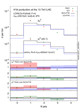
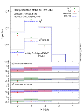
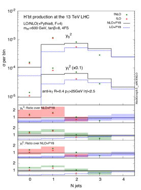
Figure 7: Same as Fig. 3, but for the jet rates (left panels) and $b$-jet rates (right panels) with $m_{H^{-}}=200\,\textrm{GeV}$ (upper panels) and $m_{H^{-}}=600\,\textrm{GeV}$ (lower panels).

Let us now conclude our 4FS study by considering jet rates, displayed in Fig. 7. In the left panel, we show jet multiplicities without requiring any $b$ tagging, while in the right panel we show $b$-jet multiplicities. First of all, we recall that in our setup the top quark decays (leptonically) both in the shower and at fixed order. For this reason, up to two/three jets and up to two $b$ jets can appear at fLO/fNLO. Looking at the $m_{H^{-}}=200\,\textrm{GeV}$ results first (upper plots), we can appreciate the effects of the NLO corrections and of the matching with parton showers. NLO effects have the largest impact in the two-jet bin, where the cross section is increased by 35% (65%) for the $y_{b}^{2}$ ($y_{t}^{2}$) term. Their effect is minor for lower multiplicities: almost no correction occurs for the $y_{b}^{2}$ term, while the $y_{t}^{2}$ one is increased by 20%. If in turn we consider the effects of the parton shower and compare the fNLO histograms to the NLO+PS ones, we infer that the main effect is to populate higher multiplicities. Therefore, the zero- and one-jet rates are reduced as a consequence of unitarity. Such a reduction is quite important, as the NLO+PY8 prediction falls outside the fNLO uncertainty band, particularly in the one-jet bin. The two-jet bin is left almost unchanged by the shower. We also find that shower effects have a much larger impact at LO, which reflects the large uncertainties associated with the LO computations, particularly at fixed order.

The distribution of events with respect to the number of $b$ jets is displayed in the upper right panel of Fig. 7. In this case NLO corrections have the largest effect on the zero- and one-$b$ jet bins. Since the majority of events lies in the one-$b$ jet bin, the shower moves events from this bin into the higher and lower multiplicities, although the effect is in general moderate and within the fNLO uncertainties. Only in the zero-$b$ jet bin, whose rate is however suppressed, the differences between fNLO and NLO+PS results are larger than in the flavour-unspecific case and the uncertainties barely overlap. Overall, the NLO predictions are reasonably close to each other, since higher multiplicities (beyond two $b$ jets) are phase-space suppressed in the NLO+PS simulations.

For both the jet and $b$-jet rates, the fraction of events with jet multiplicities beyond the ones already present at the hard-matrix element level (more than three jets and more than two $b$ jets) is in good agreement between the LO+PS and NLO+PS predictions, the LO ones being slightly enhanced though. At this point, we remark that these multiplicities are utterly Monte Carlo dependent and a substantial disagreement between Pythia8 and Herwig++ is found for these bins. For the lower multiplicities, however, their agreement is excellent, as will be discussed in detail in Sect. 3.3.

The results of Fig. 7 analysed so far are for $m_{H^{-}}=200\,\textrm{GeV}$. Since these observables are particularly relevant for experimental analyses based on jet and $b$-jet categories, let us discuss explicitly the results for a charged Higgs mass of $m_{H^{-}}=600\,\textrm{GeV}$, which are displayed in the lower plots of Fig. 7. While for jet multiplicities the general features are not so different, some specific features are. Apart from a larger Higgs mass changing the LO normalisation, the distribution of events at LO appears shifted towards low multiplicities as compared to LO+PS, without any overlap of the corresponding uncertainties in the first two bins. However, given our findings for the lower Higgs mass case, this is expected: the shower shifts events from lower towards higher jet multiplicities; this is enhanced for $m_{H^{-}}=600\,\textrm{GeV}$ due to a generally increased hardness of the process. Indeed, the two-jet bin has the largest rate, and the three- and four-jet bins are less suppressed than in the lighter Higgs case. NLO corrections slightly improve the agreement of showered and fixed-order results, albeit fNLO and NLO+PS still fall outside the respective uncertainties in the zero- and one-jet bins.

In the case of $b$ jets, on the other hand, the features of the relative curves reflect those discussed for the lighter Higgs and no further comments are needed.

3.2.2 The $y_{b}y_{t}$ contribution

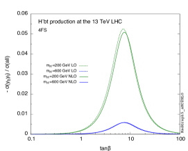
Figure 8: Relative contribution of the $y_{b}y_{t}$ term at LO (dashed) and NLO (solid) in the 4FS, with respect to the total (N)LO cross section, as a function of $\tan\beta$. The two cases $m_{H^{-}}=200\,\textrm{GeV}$ (green) and $m_{H^{-}}=600\,\textrm{GeV}$ (blue) are shown.

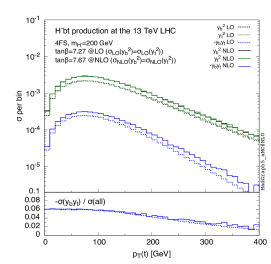
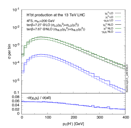
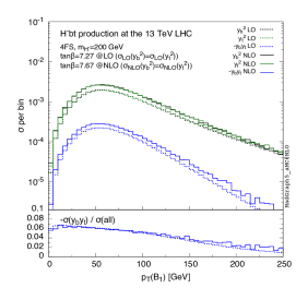
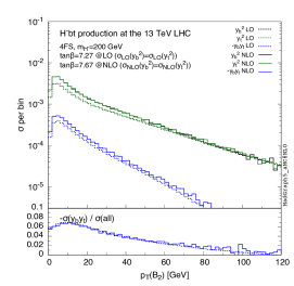
Figure 9: Differential comparisons at the between the $y_{b}y_{t}$ term and the $y_{b}^{2}$, $y_{t}^{2}$ ones, for $m_{H^{-}}=200\,\textrm{GeV}$. The transverse momentum of the top quark (top left), of the Higgs boson (top right) and of the hardest (bottom left) and second hardest (bottom right) $B$ hadron are considered. In the main frame the $y_{b}^{2}$ (black), $y_{b}^{2}$ (green) and $y_{b}y_{t}$ (blue) distribution are plotted at LO (dashed) and NLO (solid), while the inset shows the ratio $\sigma(y_{b}y_{t})/\left(\sigma(y_{b}^{2})+\sigma(y_{b}y_{t})+\sigma(y_{b}^{2})\right)$ at LO and NLO.

As we mentioned before, in the 5FS the NLO cross section receives contributions either proportional to $y_{b}^{2}$ or to $y_{t}^{2}$. No $y_{b}y_{t}$ term appears, given that it would come from the interference of left-handed with right-handed massless bottom quarks. If in turn $b$ quarks are massive, as in the 4FS, the $y_{b}y_{t}$ term does not vanish any longer, and it is proportional to $m_{b}^{2}/Q^{2}$, where $Q$ is some hard scale of the process. So far, we have limited our 4FS analysis to the $y_{b}^{2}$ and $y_{t}^{2}$ contributions, assuming the $y_{b}y_{t}$ one to be suppressed. In this section, we show that this is indeed the case.

To this purpose, we consider the total cross section for charged Higgs production in the 4FS at LO and NLO, and plot the relative contribution $-\sigma_{y_{b}y_{t}}/\sigma_{\rm all}$ as a function of $\tan\beta$ in Fig. 8, with $\sigma_{\rm all}$ being the sum of all terms. The results are shown for $m_{H^{-}}=200,600\,\textrm{GeV}$. The minus sign takes into account the fact that the $y_{b}y_{t}$ term is negative. We stress that the $y_{b}y_{t}$ contribution is independent of $\tan\beta$. As can be inferred from the plots, the relative size of the $y_{b}y_{t}$ term is below 5% for $m_{H^{-}}=200\,\textrm{GeV}$, and 0.5% for $m_{H^{-}}=600\,\textrm{GeV}$. The relative contribution to the cross section proportional to $y_{b}y_{t}$ is maximal when the $y_{b}^{2}$ and $y_{t}^{2}$ terms are equal, i. e. when

$$y_{b}^{2}\tan\beta^{2}={y_{t}^{2}}/{\tan\beta^{2}}\quad\Rightarrow\quad\tan\beta=7.27(7.67),$$ (13)

at LO (NLO), for $m_{H^{-}}=200\,\textrm{GeV}$.

Let us further investigate the potential impact of the inclusion of the $y_{b}y_{t}$ term on some differential observables, for such a value of $\tan\beta$. In particular, we look at the transverse momentum of the Higgs, the top and the two hardest $B$ hadrons for $m_{H^{-}}=200\,\textrm{GeV}$, displayed in Fig. 9. From these plots we notice that the effect of the $y_{b}y_{t}$ term is peaked at low scales, by reaching at most $6-7\%$ of the full cross section, and is almost the same at LO and NLO. We stress again that these numbers have been computed for the value of $\tan\beta$ for which the relative $y_{b}y_{t}$ contribution is maximal: for larger (smaller) values of $\tan\beta$, this contribution is suppressed by a factor $1/\tan^{2}\beta$ ($\tan^{2}\beta$) with respect to the $y_{t}^{2}$ ($y_{b}^{2}$) contribution and further reduced for heavier charged Higgs bosons. The typical scale uncertainties at NLO ($\sim 10-15\%$) justify our choice to neglect the $y_{b}y_{t}$ contribution in the current analysis. A viable alternative would be to include the relative contribution of the $y_{b}y_{t}$ term only at LO, which was shown to be very similar to the NLO one.

3.3 Four- and Five-flavour scheme comparison

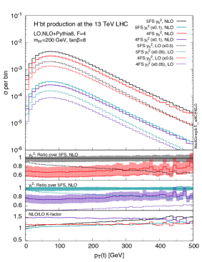
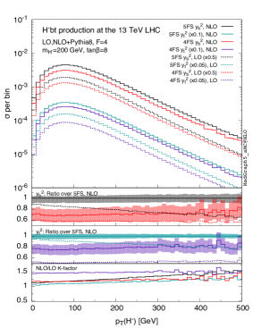
Figure 10: LO (dashed) and NLO (solid) predictions matched with Pythia8 in the 4FS (red for $y_{b}^{2}$, violet for $y_{t}^{2}$) and 5FS (black for $y_{b}^{2}$, light blue for $y_{t}^{2}$), for the transverse momentum of the top quark (left) and of the charged Higgs boson (right). Rescaling factors are introduced in the main frame for better readability. The first and second insets show the ratio over the NLO prediction in the 5FS for the $y_{b}^{2}$ and $y_{t}^{2}$ term respectively, and the scale uncertainty band for the NLO curves. The third inset show the differential $K$-factor (NLO/LO) for the four predictions. A charged Higgs boson mass $m_{H^{-}}=200\,\textrm{GeV}$ is considered.

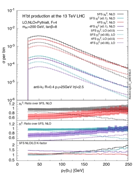
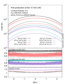
Figure 11: Same as Fig. 10, but for the transverse momentum (left) and pseudo-rapidity (right) of the hardest $b$ jet.

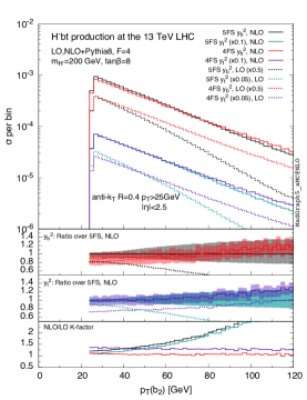
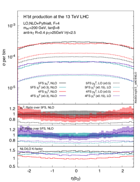
Figure 12: Same as Fig. 10, but for the transverse momentum (left) and pseudo-rapidity (right) of the second-hardest $b$ jet.

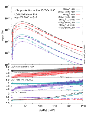
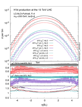
Figure 13: Same as Fig. 10, but for the transverse momentum (left) and pseudo-rapidity (right) of the hardest $B$ hadron.

We turn now to investigate how predictions obtained in the four- and five-flavours schemes compare. The two schemes are actually identical up to $b$-mass power suppressed terms when computed to all orders in perturbation theory, but the way of ordering the perturbative series is different. As a consequence, the results in the two schemes may be different at any finite order, while the inclusion of higher orders necessarily brings the predictions in the two schemes closer to each other. We start by quantifying how the inclusion of NLO corrections improves their mutual agreement. In Figs. 10-12 we show, for some relevant observables, the LO and NLO predictions (matched with Pythia8) in the two schemes. All figures have the same pattern: a main frame with the absolute predictions in the 5FS (black for $y_{b}^{2}$ and light blue for $y_{t}^{2}$) and the 4FS (red for $y_{b}^{2}$ and violet for $y_{t}^{2}$) at LO (dashed) and NLO (solid). In the first and second insets we show the ratio of the curves in the main frame over the 5FS NLO prediction, for the $y_{b}^{2}$ and $y_{t}^{2}$ contributions respectively. For the NLO predictions, a band indicating the scale uncertainty is attached to the curves. In the third inset, the four differential NLO/LO $K$-factors ($y_{b}^{2}$ and $y_{t}^{2}$ for 4FS and 5FS) are displayed.

A general observation is that, as expected, the NLO predictions in the two schemes are much closer to each other than the LO ones, in particular as far as shapes are concerned. Differences in the overall normalisation reflect the differences in the total cross section, which were already discussed in Ref. [22], while in this comparison we are mostly interested in the shapes. In Fig. 10 we observe that for the transverse momentum of the top quark and the Higgs boson the difference between the two schemes can be compensated by a simple overall rescaling of the total rates ($\sigma_{\rm tot}^{\rm 4FS}/\sigma_{\rm tot}^{\rm 5FS}\simeq 0.7$) at NLO, while LO predictions in the two schemes have considerably different shapes. The same level of agreement should be found also for observables related to the (leptonic) decay products of the top quark and the Higgs. Let us recall that in our simulation we do not decay the Higgs boson, but we decay leptonically the top quark. The $b$ quark from the top decay mostly ends up in the hardest $b$ jet. This explains why the $p_{T}$ spectrum of the hardest $b$ jet (left plot in Fig. 11) displays a flat ratio between the 4FS and 5FS at NLO, up to $\sim 120\,\textrm{GeV}$. Above that value, secondary $g\to b\bar{b}$ splittings from hard gluons become more relevant, which is also reflected in the growth of the 5FS uncertainty band and $K$-factor. A similar behaviour has been observed in the case of $tH$ production in the SM [29]. The pseudo-rapidity of the hardest $b$ jet (right plot in Fig. 11) is mostly dominated by the low-$p_{T}$ region, and it therefore also displays a good agreement between 4FS and 5FS shapes at NLO.

Larger differences between the two schemes appear for the second-hardest $b$ jet, which is expected to be poorly described in the 5FS. In particular, its kinematics in the 5FS at LO is determined by the shower, while at NLO it is driven by a tree-level matrix element (therefore being formally only LO accurate). Predictions for the transverse momentum of the second $b$ jet and its pseudo-rapidity are shown in the left and right panels of Fig. 12. The 5FS develops large $K$-factors and larger uncertainties, since its LO prediction stems only from the shower evolution. Therefore, the 4FS description has to be preferred for these observables, both because of its better perturbative behaviour and the proper modelling of the final-state $b$ jets.

The effects of the different treatment of the bottom quark in the two schemes is even more visible for the differential observables related to the hardest $B$ hadron (see Fig. 13). At medium and large $p_{T}(B_{1})$ and at central $\eta(B_{1})$ similar effects as for the hardest $b$ jet are observed. At variance, the 4FS prediction is suppressed with respect to the 5FS one at low $p_{T}(B_{1})$ and at large $\eta(B_{1})$. This is most likely due to mass effects: these kinematical regions correspond to one $b$ quark being collinear to the beam. In the 5FS these configurations are enhanced because of the collinear singularities, while in the 4FS such a singularities are screened by the $b$-quark mass. Therefore, even after the PS, the 5FS is reminiscent of the collinear enhancement. In the case of the second-hardest $B$ hadron (not shown) these effects are further enhanced.

Let us make a final remark on the inclusion of the NLO corrections. The NLO/LO $K$-factor is quite different in the two schemes: in the 4FS the $K-$factor appears much more pronounced for the $y_{t}^{2}$ than for the $y_{b}^{2}$ term, while in the 5FS it is similar for both contributions. Despite that, a remarkable compensation in shape between the LO differential cross sections and the NLO corrections takes place, such that the 4FS/5FS ratio at NLO is quite similar for the $y_{b}^{2}$ and $y_{t}^{2}$ terms.

All the plots discussed so far are relevant to the lighter Higgs under consideration ($m_{H^{-}}=200\,\textrm{GeV}$). For a heavier charged Higgs boson ($m_{H^{-}}=600\,\textrm{GeV}$), the picture does not change significantly. The only thing that may be worth mentioning is the fact that, for the second $b$ jet, the $K$-factor in the 5FS lies much closer to unity than for the lighter Higgs. Such a behaviour may be due to the increased weight of the initial-state collinear logarithms resummed by the bottom PDFs in the 5FS, which are enhanced at larger masses of the produced particle. Besides, as already pointed out in Ref. [23], collinear logarithms become increasingly relevant the larger the fraction of the momentum carried by the initial partons is.

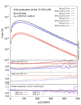
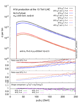
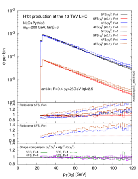
Figure 14: 4FS (blue for the $y_{b}^{2}$ term, orange for the $y_{t}^{2}$ one) and 5FS (black for the $y_{b}^{2}$ term, red for the $y_{t}^{2}$ one) distributions for the transverse momentum of the top (left) and charged Higgs (right), for $m_{H^{-}}=200\,\textrm{GeV}$; the $F=1$ (dashed) and $F=4$ (solid) predictions are shown. The first inset shows the ratios of the histogram in the main frame over the 5FS, $F=4$ prediction. The second inset shows the ratios of the $F=1$ histograms over the corresponding 5FS ones. The third inset shows the ratio of the normalised $y_{b}^{2}$ histograms in the main frame over the corresponding $y_{t}^{2}$ ones.

Figure 15: Same as Fig. 15, but for the transverse momentum of the hardest (left) and second-hardest (right) $b$ jet .

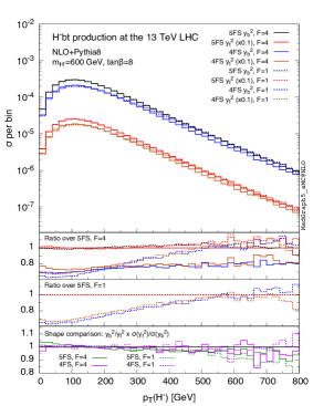
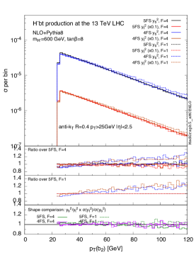
Figure 16: Same as Fig. 15, but for transverse momentum distribution of the top (left) and the second-hardest $b$ jet (right) with $m_{H^{-}}=600\,\textrm{GeV}$.

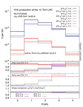
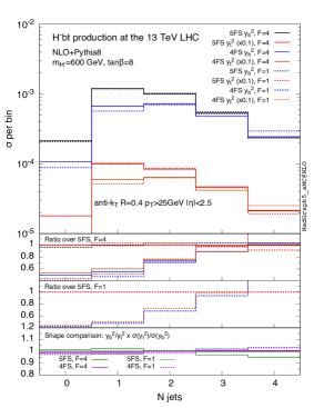
Figure 17: Same as Fig. 15, but for the jet multiplicity with $m_{H^{-}}=200\,\textrm{GeV}$ (left) and $m_{H^{-}}=600\,\textrm{GeV}$ (right).

We continue our analysis by investigating how the choice of the shower scale affects the results in the two schemes. We stress once more that our default choice ($F=4$) is physically well-motivated by the arguments given in Sect. 3.1. Below we show that this choice also improves the mutual agreement between the NLO predictions in the two schemes. A number of differential distributions in the 4FS and 5FS for $F=1$ and $F=4$ are shown in Figs. 15-17, for both $m_{H^{-}}=200\,\textrm{GeV}$ and $600\,\textrm{GeV}$. The main frame displays predictions in the 5FS for the $y_{b}^{2}$ term (black) and $y_{t}^{2}$ term (red) as well as in the 4FS (in blue and orange respectively). Solid curves are used for our reference predictions with $F=4$, while dashed curves refer to the default choice in MadGraph5_aMC@NLO ($F=1$). The first inset displays the ratio of the curves in the main frame over the corresponding ones ($y_{b}^{2}$ or $y_{t}^{2}$) in the 5FS for $F=4$. The second inset shows the ratio of the curves with $F=1$ in the 4FS over the corresponding ones in the 5FS. In these two insets we can analyse whether $F=1$ or $F=4$ yields a flatter 4FS/5FS ratio. In the last inset, the ratio of the normalised $y_{b}^{2}$ and $y_{t}^{2}$ distributions is plotted, for the 4FS and 5FS and for $F=1,4$. The purpose of this inset is to study whether the $y_{t}^{2}$ and $y_{b}^{2}$ contributions develop similar shapes.

Overall, we observe a smaller dependence on $F$ in the 5FS than in the 4FS distributions. A similar behaviour was found in the context of Higgs production in association with bottom quarks [28]. In any case, the choice of $F$ is almost irrelevant when considering observables that are not sensitive to the $b$-quark degrees of freedom. In Fig. 15, where $m_{H^{-}}=200\,\textrm{GeV}$, we notice that charged Higgs and top $p_{T}$ distributions are slightly harder in the 4FS (10-15% at large $p_{T}$) for $F=1$. Moreover, the $F=4$ choice yields a remarkably flat 4FS/5FS ratio, much flatter than for $F=1$. Consequently, $F=4$ improves the agreement between the two schemes.

This improvement becomes even more visible for observables sensitive to the $b$ kinematics. For example, Fig. 15 shows the transverse momentum of the hardest (left panel) and second-hardest (right panel) $b$ jet, where $F=1$ provides much harder spectra in the 4FS than $F=4$. A similar pattern is visible in the case of $B$ hadrons. In this case, however, the general agreement between 4FS and 5FS significantly deteriorates, as it was already observed.

In general, similar conclusions can be drawn for $m_{H^{-}}=600\,\textrm{GeV}$. The only two distributions that exhibit a different behaviour as compared to the $m_{H^{-}}=200\,\textrm{GeV}$ case are shown in Fig. 16. The transverse momentum distribution of the heavy charged Higgs boson (left panel) in the 4FS is much more affected by the choice of $F$, with effects that reach up to 40% in the tail of the distribution. In this case the 4FS and 5FS mutual agreement is significantly improved by the choice $F=4$. The transverse momentum distribution of the second-hardest $b$ jet (right panel) is less sensitive to the choice of $F$ than in the lighter-Higgs scenario.

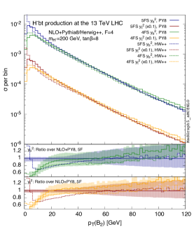
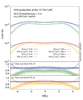
Figure 18: Transverse momentum (left) and pseudo-rapidity (right) distribution of the second-hardest $B$ hadron. NLO curves matched with Pythia8 (solid) and Herwig++ (dashed) are shown, in the 5FS (blue for the $y_{b}^{2}$ term, dark-red for the $y_{t}^{2}$ one) and 4FS (green for the $y_{b}^{2}$ term, light-orange for the $y_{t}^{2}$ one). The two insets show the ratios of the histogram in the main frame over the 5FS prediction matched with Pythia8, for the $y_{b}^{2}$ and $y_{t}^{2}$ terms separately. Scale uncertainty bands are shown around the Pythia8 predictions.

Jet multiplicities are a class of observables that are particularly sensitive to the excess of radiation generated by using $F=1$. From Fig. 17 we conclude that the 4FS generally prefers higher jet multiplicities than the 5FS. A similar behaviour was observed also in Ref. [29] and it was explained by considering the different colour structure of the initial state in the two schemes, besides the fact that the process is generally harder in the 4FS. This tendency is slightly reduced—and as a consequence the agreement slightly improves—by the choice of a smaller shower scale ($F=4$). We remark that the dependence on the shower scale is even less apparent in the heavy charged Higgs case, and for $b$-jet multiplicities (not shown).

Finally, the ratio between the $y_{b}^{2}$ and $y_{t}^{2}$ terms (last insets of Figs. 15-17) illustrates that the two contributions give remarkably similar shapes for all observables under consideration. Any difference emerges from the dynamical scale choice at which the bottom Yukawa is computed ($\bar{m}_{b}(\mu_{R})$ with $\mu_{R}=H_{T}/3$, see Sect. 3.1). However, such difference is never larger than 10%, with the $y_{b}^{2}$ distributions being slightly softer than the $y_{t}^{2}$ ones.

Finally, we analyse the sensitivity of various observables to the parton shower in the four- and five-flavour schemes. To this purpose, we compare results at NLO matched with the Pythia8 and Herwig++ Monte Carlos. Having verified that the relative behaviour of the two Monte Carlos hardly depends on the specific choice of the charged Higgs mass under consideration, we limit the discussion to the $m_{H^{-}}=200\,\textrm{GeV}$ results.

As already pointed out in the introduction, the parton-shower matching for bottom-quark initial states in the 5FS involves some approximations: the initial-state backward evolution is based on leading-log accurate gluon splittings and requires the reshuffling of massless into massive bottom quarks. For these reasons, the 5FS predictions are extremely sensitive to the specific treatment of bottom quarks in a given Monte Carlo. This is most remarkable for $b$-jet/$B$-hadron related observables, such as the transverse momentum distribution of the second-hardest $B$ hadron (displayed in the left panel of Fig. 18). In the 5FS, the Herwig++ prediction displays a significant shape distortion, both at small and large values of the transverse momentum, falling outside the Pythia8 uncertainty bands at small $p_{T}$. A similar discrepancy is evident in the forward region of the rapidity spectrum, shown in the right panel of Fig. 18. In this plot, the 5FS prediction is larger for Herwig++ than for Pythia8. For both observables, the 4FS results display a significantly smaller Monte Carlo dependence.

An even more spectacular example is provided by the $\eta-\phi$ distance between the two hardest $B$ hadrons. The results are shown in the left panel of Fig. 20. The Herwig++ prediction in the 5FS features a much higher tail at large separations. This can be traced back to the fact that Herwig++ tends to produce $B$ hadrons much closer to the beam line when simulations are performed in the 5FS. The same behaviour was observed in Ref. [28], in which it was pointed out that such effects are however not relevant when realistic cuts on the $B$ hadrons are imposed, for example, when $b$ jets are required. As a matter of fact, we observe a neatly improved agreement among all curves in Fig. 20 when requiring at least two $b$ jets (right panel).

Looking further at jet (left panel) and $b$-jet (right panel) multiplicities in Fig. 20, we observe instead that the two flavour-schemes display a similar Monte Carlo dependence. In the flavour–unspecific case this dependence is quite small for all jet-multiplicity bins. On the other hand, for $b$ jets Herwig++ and Pythia8 are in good agreement up to one $b$ jet in the 5FS and two $b$ jets in the 4FS, that is up to the multiplicities described by the hard matrix element at NLO. The two $b$-jet bin in the 5FS—described only at LO by the hard matrix element—is affected by larger discrepancies between the two Monte Carlos, which exceed the uncertainty bands. Larger $b$-jet multiplicities, generated only at the shower level via gluon splittings, are affected by discrepancies as large as 100%: Herwig++ predicts less $b$ jets than Pythia8.

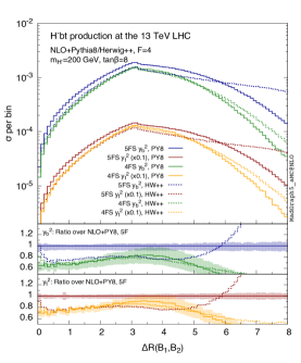
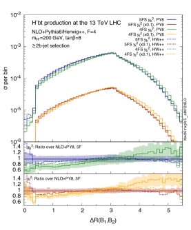
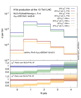
Figure 19: Same as Fig. 18, but for the $\eta-\phi$ distance of the two hardest $B$ hadrons with no cuts (left) and requiring at least two $b$ jets (right).

Figure 20: Same as Fig. 18, but for the jet (left) and $b$-jet (right) multiplicity.

Generally speaking, the difference between the Monte Carlos is smaller for the 4FS than for 5FS predictions. Indeed, the 4FS has more differential information at the matrix-element level, which reduces the effects of the shower. The only case worth mentioning, in which the Monte Carlo dependence is larger in the 4FS than in the 5FS is the distance between two hardest $b$ jets at large separations. This observable is closely related to the distance of the two hardest $B$ hadrons when two $b$ jets are required (see right panel in Fig. 20). For both observables, at large separations, the 4FS predictions matched with Herwig++ lie very close to the 5FS NLO+PS predictions, while the matching with Pythia8 yields a higher tail. However, we point out that such discrepancy between Herwig++ and Pythia8 in the 4FS barely exceeds the scale uncertainty bands.

Finally, we remark that similar conclusions can be drawn for the heavier charged Higgs case for most of the studied observables. However, a heavier charged Higgs reduces the differences between the two Monte Carlos (in particular in the 5FS) in the transverse momentum distribution of the two hardest $B$ hadrons/$b$ jets.

4 Conclusions

We have presented predictions for the production of a heavy charged Higgs boson in a type-II 2HDM, by explicitly considering a lighter Higgs scenario ($m_{H^{-}}$ = 200 GeV) and a heavier one ($m_{H^{-}}$ = 600 GeV). Our predictions have been presented for $\tan\beta=8$, but they are applicable to any $\tan\beta$ value through a simple rescaling. Furthermore, these results can be straightforwardly extended to a type-I 2HDM by rescaling the Yukawa couplings. Details are given in Sect. 6 of Ref. [22].

For the first time, a fully differential computation has been performed in the 4FS at fNLO and NLO+PS accuracy. We have exploited the automatised MadGraph5_aMC@NLO framework, by obtaining the NLO version of the 2HDM via the NLOCT package. The model has been supplemented by the computation of the bottom Yukawa coupling in the $\overline{\text{MS}}$ scheme, which has the advantage with respect to the default on-shell scheme of resumming large logarithms of $m_{b}/\mu_{R}$.

Our results indicate that a reduced shower scale with respect to the default one in MadGraph5_aMC@NLO improves the matching between parton shower and fixed-order results at large transverse momenta. For this scale choice, we discussed the effects of incorporating NLO corrections and the matching to the parton shower in the 4FS simulations by considering a number of differential observables. We found NLO corrections to be generally flat with our choice of the renormalisation and factorisation scales. Effects due to the parton shower are important in the Sudakov-dominated regions (jets and $B$ hadrons at low $p_{T}$), or when observables sensitive to the $b$-quark fragmentation are considered. These observations have been made separately for the $y_{b}^{2}$ and $y_{t}^{2}$ terms. On the other hand, we argued that the $y_{b}y_{t}$ contribution, appearing only in the 4FS, can be safely neglected, since its size is smaller than $\sim 5$% of the total cross section (for $\tan\beta=8$ and $m_{H^{-}}=200$ GeV) and is well within the scale uncertainty of the computation. For larger Higgs masses or different values of $\tan\beta$ it is further suppressed.

Besides discussing the new results in the 4FS, we provided a comprehensive comparison to the ones in the 5FS, consistently generated within MadGraph5_aMC@NLO. The inclusion of NLO(+PS) corrections in the two schemes improves their mutual agreement at the level of shapes. This agreement follows, although to a minor extent, from the reduced shower scale choice. Differences remain, however, and they are particularly sizeable for observables related to $b$ jets and $B$ hadrons. Given these differences, it was vital to carry out an unbiased analysis of our results in order to acquire the most reliable predictions for this class of observables. The proper simulation of the signal will be crucial for the experiments to fully exploit the potential of the data collected in charged Higgs searches at the LHC.

Our final recommendation is to use 4FS predictions for any realistic signal simulation in experimental searches. This recommendation is backed by two sets of evidences: first we have proven that, for a large number of observables, the 4FS prediction provides a better description of the final state kinematics; second, it reduces the systematic error related to the usage of a given parton shower. Moreover, when matching the NLO calculation to the shower, we recommend to use a lower shower scale (by setting $F=4$ in our case). This choice provides a better matching to the fixed-order computation at large transverse momenta, slightly reduces the parton shower dependence and improves the agreement of four- and five-flavour scheme computations.

Any user interested in the simulation of charged Higgs production with MadGraph5_aMC@NLO is strongly encouraged to contact the authors.

References

- [1] ALEPH, DELPHI, L3, OPAL, LEP Collaboration, G. Abbiendi et al., Search for Charged Higgs bosons: Combined Results Using LEP Data, Eur.Phys.J. C73 (2013) 2463, [arXiv:1301.6065].
- [2] CDF Collaboration, T. Aaltonen et al., Search for charged Higgs bosons in decays of top quarks in p- collisions at TeV, Phys. Rev. Lett. 103 (2009) 101803, [arXiv:0907.1269].
- [3] D0 Collaboration, V. M. Abazov et al., Search for charged Higgs bosons in top quark decays, Phys. Lett. B 682 (2009) 278, [arXiv:0908.1811].
- [4] ATLAS Collaboration, G. Aad et al., Search for charged Higgs bosons decaying via in fully hadronic final states using collision data at TeV with the ATLAS detector, JHEP 1503 (2015) 088, [arXiv:1412.6663].
- [5] CMS Collaboration, Search for charged Higgs bosons with the H+ to tau nu decay channel in the fully hadronic final state at TeV, Tech. Rep. CMS-PAS-HIG-14-020, CERN, Geneva, 2014.
- [6] CMS Collaboration, Search for a light charged Higgs boson in top quark decays in pp collisions at = 7 TeV, JHEP 1207 (2012) 143, [arXiv:1205.5736].
- [7] CMS Collaboration, Search for a heavy charged Higgs boson in proton-proton collisions at sqrts=8 TeV with the CMS detector, Tech. Rep. CMS-PAS-HIG-13-026, CERN, Geneva, 2014.
- [8] C. Degrande, R. Frederix, M. Ubiali, M. Wiesemann, and M. Zaro, in preparation, .
- [9] W. Peng, M. Wen-Gan, Z. Ren-You, J. Yi, H. Liang, and G. Lei, NLO supersymmetric QCD corrections to the associated production at hadron colliders, Phys.Rev. D73 (2006) 015012, [hep-ph/0601069].
- [10] S. Dittmaier, M. Kramer, M. Spira, and M. Walser, Charged-Higgs-boson production at the LHC: NLO supersymmetric QCD corrections, Phys.Rev. D83 (2011) 055005, [arXiv:0906.2648].
- [11] S.-h. Zhu, Complete next-to-leading order QCD corrections to charged Higgs boson associated production with top quark at the CERN large hadron collider, Phys.Rev. D67 (2003) 075006, [hep-ph/0112109].
- [12] G. Gao, G. Lu, Z. Xiong, and J. Yang, Loop effects and nondecoupling property of SUSY QCD in , Phys.Rev. D66 (2002) 015007, [hep-ph/0202016].
- [13] T. Plehn, Charged Higgs boson production in bottom gluon fusion, Phys.Rev. D67 (2003) 014018, [hep-ph/0206121].
- [14] E. L. Berger, T. Han, J. Jiang, and T. Plehn, Associated production of a top quark and a charged Higgs boson, Phys.Rev. D71 (2005) 115012, [hep-ph/0312286].
- [15] N. Kidonakis, Charged Higgs production: Higher-order corrections, PoS HEP2005 (2006) 336, [hep-ph/0511235].
- [16] C. Weydert, S. Frixione, M. Herquet, M. Klasen, E. Laenen, T. Plehn, G. Stavenga, and C. D. White, Charged Higgs boson production in association with a top quark in MC@NLO, Eur.Phys.J. C67 (2010) 617–636, [arXiv:0912.3430].
- [17] M. Klasen, K. Kovarik, P. Nason, and C. Weydert, Associated production of charged Higgs bosons and top quarks with POWHEG, Eur.Phys.J. C72 (2012) 2088, [arXiv:1203.1341].
- [18] M. Beccaria, G. Macorini, L. Panizzi, F. Renard, and C. Verzegnassi, Associated production of charged Higgs and top at LHC: The Role of the complete electroweak supersymmetric contribution, Phys.Rev. D80 (2009) 053011, [arXiv:0908.1332].
- [19] D. T. Nhung, W. Hollik, and L. D. Ninh, Electroweak corrections to at the LHC, Phys.Rev. D87 (2013) 113006, [arXiv:1210.4087].
- [20] N. Kidonakis, Charged Higgs production via bg at the LHC, JHEP 0505 (2005) 011, [hep-ph/0412422].
- [21] N. Kidonakis, Two-loop soft anomalous dimensions for single top quark associated production with a W- or H-, Phys.Rev. D82 (2010) 054018, [arXiv:1005.4451].
- [22] M. Flechl, R. Klees, M. Kramer, M. Spira, and M. Ubiali, Improved cross-section predictions for heavy charged Higgs boson production at the LHC, Phys.Rev. D91 (2015), no. 7 075015, [arXiv:1409.5615].
- [23] F. Maltoni, G. Ridolfi, and M. Ubiali, b-initiated processes at the LHC: a reappraisal, JHEP 1207 (2012) 022, [arXiv:1203.6393].
- [24] M. Ubiali, Are bottom PDFs needed at the LHC?, PoS DIS2014 (2014) 037.
- [25] R. Harlander, M. Kramer, and M. Schumacher, Bottom-quark associated Higgs-boson production: reconciling the four- and five-flavour scheme approach, CERN-PH-TH-2011-134 (2011) [arXiv:1112.3478].
- [26] S. Dawson, A. Ismail, and I. Low, A Redux on ”When is the Top Quark a Parton?”, Phys.Rev. D90 (2014) 014005, [arXiv:1405.6211].
- [27] S. Frixione, F. Stoeckli, P. Torrielli, and B. R. Webber, NLO QCD corrections in Herwig++ with MC@NLO, JHEP 1101 (2011) 053, [arXiv:1010.0568].
- [28] M. Wiesemann, R. Frederix, S. Frixione, V. Hirschi, F. Maltoni, and P. Torrielli, Higgs production in association with bottom quarks, JHEP 1502 (2015) 132, [arXiv:1409.5301].
- [29] F. Demartin, F. Maltoni, K. Mawatari, and M. Zaro, Higgs production in association with a single top quark at the LHC, arXiv:1504.00611.
- [30] J. M. Campbell, R. Frederix, F. Maltoni, and F. Tramontano, Next-to-Leading-Order Predictions for t-Channel Single-Top Production at Hadron Colliders, Phys.Rev.Lett. 102 (2009) 182003, [arXiv:0903.0005].
- [31] R. Frederix, E. Re, and P. Torrielli, Single-top t-channel hadroproduction in the four-flavour scheme with POWHEG and aMC@NLO, JHEP 1209 (2012) 130, [arXiv:1207.5391].
- [32] J. Alwall, R. Frederix, S. Frixione, V. Hirschi, F. Maltoni, O. Mattelaer, H.-S. Shao, T. Stelzer, P. Torielli, and M. Zaro, The automated computation of tree-level and next-to-leading order differential cross sections, and their matching to parton shower simulations, JHEP 1407 (2014) 079, [arXiv:1405.0301].
- [33] G. Ossola, C. G. Papadopoulos, and R. Pittau, On the Rational Terms of the one-loop amplitudes, JHEP 0805 (2008) 004, [arXiv:0802.1876].
- [34] C. Degrande, Automatic evaluation of UV and R2 terms for beyond the Standard Model Lagrangians: a proof-of-principle, arXiv:1406.3030.
- [35] FeynRules 2.0 - A complete toolbox for tree-level phenomenology, Comput.Phys.Commun. 185 (2014) 2250–2300, [arXiv:1310.1921].
- [36] T. Hahn, Generating Feynman diagrams and amplitudes with FeynArts 3, Comput.Phys.Commun. 140 (2001) 418–431, [hep-ph/0012260].
- [37] C. Degrande, C. Duhr, B. Fuks, D. Grellscheid, O. Mattelaer, et al., UFO - The Universal FeynRules Output, Comput.Phys.Commun. 183 (2012) 1201–1214, [arXiv:1108.2040].
- [38] H. Murayama, I. Watanabe, and K. Hagiwara, HELAS: HELicity amplitude subroutines for Feynman diagram evaluations, .
- [39] P. de Aquino, W. Link, F. Maltoni, O. Mattelaer, and T. Stelzer, ALOHA: Automatic Libraries Of Helicity Amplitudes for Feynman Diagram Computations, Comput.Phys.Commun. 183 (2012) 2254–2263, [arXiv:1108.2041].
- [40] S. Frixione, Z. Kunszt, and A. Signer, Three jet cross-sections to next-to-leading order, Nucl.Phys. B467 (1996) 399–442, [hep-ph/9512328].
- [41] S. Frixione, A General approach to jet cross-sections in QCD, Nucl.Phys. B507 (1997) 295–314, [hep-ph/9706545].
- [42] R. Frederix, S. Frixione, F. Maltoni, and T. Stelzer, Automation of next-to-leading order computations in QCD: The FKS subtraction, JHEP 0910 (2009) 003, [arXiv:0908.4272].
- [43] V. Hirschi, R. Frederix, S. Frixione, M. V. Garzelli, F. Maltoni, and R. Pittau, Automation of one-loop QCD corrections, JHEP 1105 (2011) 044, [arXiv:1103.0621].
- [44] G. Ossola, C. G. Papadopoulos, and R. Pittau, Reducing full one-loop amplitudes to scalar integrals at the integrand level, Nucl.Phys. B763 (2007) 147–169, [hep-ph/0609007].
- [45] G. Passarino and M. Veltman, One Loop Corrections for Annihilation into in the Weinberg Model, Nucl.Phys. B160 (1979) 151.
- [46] A. I. Davydychev, A Simple formula for reducing Feynman diagrams to scalar integrals, Phys.Lett. B263 (1991) 107–111.
- [47] G. Ossola, C. G. Papadopoulos, and R. Pittau, CutTools: A Program implementing the OPP reduction method to compute one-loop amplitudes, JHEP 0803 (2008) 042, [arXiv:0711.3596].
- [48] H.-S. Shao, IREGI user manual, unpublished.
- [49] F. Cascioli, P. Maierhofer, and S. Pozzorini, Scattering Amplitudes with Open Loops, Phys.Rev.Lett. 108 (2012) 111601, [arXiv:1111.5206].
- [50] S. Frixione and B. R. Webber, Matching NLO QCD computations and parton shower simulations, JHEP 0206 (2002) 029, [hep-ph/0204244].
- [51] G. Corcella, I. Knowles, G. Marchesini, S. Moretti, K. Odagiri, P. Richardson, M. H. Seymour, and B. R. Webber, HERWIG 6: An Event generator for hadron emission reactions with interfering gluons (including supersymmetric processes), JHEP 0101 (2001) 010, [hep-ph/0011363].
- [52] T. Sjostrand, S. Mrenna, and P. Z. Skands, PYTHIA 6.4 Physics and Manual, JHEP 0605 (2006) 026, [hep-ph/0603175].
- [53] M. Bahr, S. Gieseke, M. Gigg, D. Grellscheid, K. Hamilton, O. Latunde-Dada, S. Platzer, P. Richardson, M. H. Seymour, A. Sherstnev, and B. R. Webber, Herwig++ Physics and Manual, Eur.Phys.J. C58 (2008) 639–707, [arXiv:0803.0883].
- [54] T. Sjostrand, S. Mrenna, and P. Z. Skands, A Brief Introduction to PYTHIA 8.1, Comput.Phys.Commun. 178 (2008) 852–867, [arXiv:0710.3820].
- [55] J. Alwall, E. Boos, L. Dudko, M. Gigg, M. Herquet, A. Pukhov, P. Richardson, A. Sherstnev, and P. Z. Skands, A Les Houches Interface for BSM Generators, arXiv:0712.3311.
- [56] R. Frederix, S. Frixione, V. Hirschi, F. Maltoni, R. Pittau, and P. Torielli, Four-lepton production at hadron colliders: aMC@NLO predictions with theoretical uncertainties, JHEP 1202 (2012) 099, [arXiv:1110.4738].
- [57] NNPDF Collaboration, R. D. Ball et al., Parton distributions with LHC data, Nucl.Phys. B867 (2013) 244–289, [arXiv:1207.1303].
- [58] NNPDF Collaboration, R. D. Ball et al., Parton distributions for the LHC Run II, JHEP 1504 (2015) 040, [arXiv:1410.8849].
- [59] M. Cacciari, G. P. Salam, and G. Soyez, The Anti-k(t) jet clustering algorithm, JHEP 0804 (2008) 063, [arXiv:0802.1189].
- [60] M. Cacciari, G. P. Salam, and G. Soyez, FastJet User Manual, Eur.Phys.J. C72 (2012) 1896, [arXiv:1111.6097].
- [61] M. Cacciari and G. P. Salam, Dispelling the myth for the jet-finder, Phys.Lett. B641 (2006) 57–61, [hep-ph/0512210].
- [62] P. Artoisenet, R. Frederix, O. Mattelaer, and R. Rietkerk, Automatic spin-entangled decays of heavy resonances in Monte Carlo simulations, JHEP 1303 (2013) 015, [arXiv:1212.3460].