subref subname = section  thmref thmname = theorem  lemref lemname = lemma 

Extensions of Positive Definite Functions: Applications and Their Harmonic Analysis

Palle E.T. Jorgensen Department of Mathematics The University of Iowa Iowa City, IA 52242-1419, U.S.A. Email address: palle-jorgensen@uiowa.edu URL: http://www.math.uiowa.edu/~jorgen/

Steen Pedersen Department of Mathematics Wright State University Dayton, OH 45435, U.S.A. E-mail address: steen.math@gmail.com, steen@math.wright.edu URL: http://www.wright.edu/~steen.pedersen/

Feng Tian Department of Mathematics Trine University One University Avenue, Angola, IN 46703, U.S.A. E-mail address: james.ftian@gmail.com, tianf@trine.edu

Dedicated to the memory of

William B. Arveson

(22 November 1934 – 15 November 2011)

Edward Nelson

(May 4, 1932 – September 10, 2014)

We study two classes of extension problems, and their interconnections:

1. Extension of positive definite (p.d.) continuous functions defined on subsets in locally compact groups $G$;

2. In case of Lie groups, representations of the associated Lie algebras $La\left(G\right)$ by unbounded skew-Hermitian operators acting in a reproducing kernel Hilbert space (RKHS) $\mathscr{H}_{F}$.

Our analysis is non-trivial even if $G=\mathbb{R}^{n}$, and even if $n=1$. If $G=\mathbb{R}^{n}$, we are concerned in (ii) with finding systems of strongly commuting selfadjoint operators $\left\{T_{i}\right\}$ extending a system of commuting Hermitian operators with common dense domain in $\mathscr{H}_{F}$.

Why extensions? In science, experimentalists frequently gather spectral data in cases when the observed data is limited, for example limited by the precision of instruments; or on account of a variety of other limiting external factors. (For instance, the human eye can only see a small portion of the electromagnetic spectrum.) Given this fact of life, it is both an art and a science to still produce solid conclusions from restricted or limited data. In a general sense, our monograph deals with the mathematics of extending some such given partial data-sets obtained from experiments. More specifically, we are concerned with the problems of extending available partial information, obtained, for example, from sampling. In our case, the limited information is a restriction, and the extension in turn is the full positive definite function (in a dual variable); so an extension if available will be an everywhere defined generating function for the exact probability distribution which reflects the data; if it were fully available. Such extensions of local information (in the form of positive definite functions) will in turn furnish us with spectral information. In this form, the problem becomes an operator extension problem, referring to operators in a suitable reproducing kernel Hilbert spaces (RKHS). In our presentation we have stressed hands-on-examples. Extensions are almost never unique, and so we deal with both the question of existence, and if there are extensions, how they relate back to the initial completion problem.

By a theorem of S. Bochner, the continuous p.d. functions are precisely the Fourier transforms of finite positive measures. In the case of locally compact Abelian groups $G$, the two sides in the Fourier duality is that of the group $G$ itself vs the dual character group $\widehat{G}$ to $G$. Of course if $G=\mathbb{R}^{n}$, we may identify the two.

But in practical applications a p.d. function will typically be given only locally, or on some open subset, typically bounded; say an interval if $G=\mathbb{R}^{1}$; or a square or a disk in case $G=\mathbb{R}^{2}$. Hence four questions naturally arise:

1. Existence of extensions.

2. If there are extensions, find procedures for constructing them.

3. Moreover, what is the significance of choice of different extensions from available sets of p.d. extensions?

4. Finally, what are the generalizations and applications of the results in (a)-(c) to the case of an infinite number of dimensions?

All four questions will be addressed, and the connections between (d) and probability theory will be stressed.

While the theory of p.d. functions is important in many areas of pure and applied mathematics, ranging from harmonic analysis, functional analysis, spectral theory, representations of Lie groups, and operator theory on the pure side, to such applications as mathematical statistics, to approximation theory, to optimization (and more, see details below), and to quantum physics, it is difficult for students and for the novice to the field, to find accessible presentations in the literature which cover all these disparate points of view, as well as stressing common ideas and interconnections.

We have aimed at filling this gap, and with a minimum number of prerequisites. We do expect that readers have some familiarity with measures and their Fourier transform, as well as with operators in Hilbert space, especially the theory of unbounded symmetric operators with dense domain. When needed, we have included brief tutorials. Further, in our cited references we have included both research papers, and books. To help with a historical perspective, we have included discussions of some landmark presentations, especially papers of S. Bochner, M.G. Krein, J. von Neumann, W. Rudin, and I.J. Schöenberg.

The significance to stochastic processes of the two questions, (i) and (ii) above, is as follows. To simplify, consider first stochastic processes $X_{t}$ indexed by time $t$, but known only for “small” $t$. Then the corresponding covariance function $c_{X}\left(s,t\right)$ will also only be known for small values of $s$ and $t$; or in the case of stationary processes, there is then a locally defined p.d. function $F$, known only in a bounded interval $J=\left(-a,a\right)$, and such that $F\left(s-t\right)=c_{X}\left(s,t\right)$. Hence, it is natural to ask how much can be said about extensions to values of $t$ in the complement of $J$? For example; what are the possible global extensions $X_{t}$, i.e., extension to all $t\in\mathbb{R}$? If there are extensions, then how does information about the locally defined covariance function influence the extended global process? What is the structure of the set of all extensions? The analogues questions are equally interesting for processes indexed by groups more general than $\mathbb{R}$.

Specifically, we consider partially defined p.d. continuous functions $F$ on a fixed group. From $F$ we then build a RKHS $\mathscr{H}_{F}$, and the operator extension problem is concerned with operators acting in $\mathscr{H}_{F}$, and with unitary representations of $G$ acting on $\mathscr{H}_{F}$. Our emphasis is on the interplay between the two problems, and on the harmonic analysis of our RKHS $\mathscr{H}_{F}$.

In the cases of $G=\mathbb{R}^{n}$, and $G=\mathbb{R}^{n}/\mathbb{Z}^{n}$, and generally for locally compact Abelian groups, we establish a new Fourier duality theory; including for $G=\mathbb{R}^{n}$ a time/frequency duality, where the extension questions (i) are in time domain, and extensions from (ii) in frequency domain. Specializing to $n=1$, we arrive of a spectral theoretic characterization of all skew-Hermitian operators with dense domain in a separable Hilbert space, having deficiency-indices $\left(1,1\right)$.

Our general results include non-compact and non-Abelian Lie groups, where the study of unitary representations in $\mathscr{H}_{F}$ is subtle.

While, in the most general case, the obstructions to extendibility (of locally defined positive definite (p.d.) functions) is subtle, we point out that it has several explicit features: algebraic, analytic, and geometric. In Section 19, we give a continuous p.d. function $F$ in a neighborhood of $0$ in $\mathbb{R}^{2}$ for which $Ext\left(F\right)$ is empty. In this case, the obstruction for $F$, is geometric in nature; and involves properties of a certain Riemann surface. (See Figure 1, and Section 19, Figures 19-20, for details.)

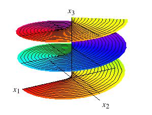
Figure 1: Riemann Surface of $\log z$.

Note on Presentation. In presenting our results, we have aimed for a reader-friendly account. We have found it helpful to illustrate the ideas with worked examples. Each of our theorems holds in various degrees of generality, but when appropriate, we have not chosen to present details in their highest level of generality. Rather, we typically give the result in a setting where the idea is more transparent, and easier to grasp. We then work the details systematically at this lower level of generality. But we also make comments about the more general versions; sketching these in rough outline. The more general versions of the respective theorems will typically be easy for readers to follow, and to appreciate, after the idea has already been fleshed out in a simpler context.

We have made a second choice in order to make it easier for students to grasp the ideas as well as the technical details: We have included a lot of worked examples. And at the end of each of these examples, we then outline how the specific details (from the example in question) serve to illustrate one or more features in the general theorems elsewhere in the monograph. Finally, we have made generous use of both Tables and Figures. These are listed with page-references at the end of the book; see the last few items in the Table of Contents. And finally, we included a list of Symbols on page Symbols, after Table of Contents.

The art of doing mathematics consists in finding that special case which contains all the germs of generality. — David Hilbert

On the one hand, the subject of positive definite (p.d.) functions has played an important role in standard graduate courses, and in research papers, over decades; and yet when presenting the material for a particular purpose, the authors have found that there is not a single source which will help students and researchers quickly form an overview of the essential ideas involved. Over the decades new ideas have been incorporated into the study of p.d. functions, and their more general cousin, p.d. kernels, from a host of diverse areas. An influence of more recent vintage is the theory of operators in Hilbert space, and their spectral theory.

A novelty in our present approach is the use of diverse Hilbert spaces. In summary; starting with a locally defined p.d. $F$, there is a natural associated Hilbert space, arising as a reproducing kernel Hilbert space (RKHS), $\mathscr{H}_{F}$. Then the question is: When is it possible to realize globally defined p.d. extensions of $F$ with the use of spectral theory for operators in the initial RKHS, $\mathscr{H}_{F}$? And when will it be necessary to enlarge the Hilbert space, i.e., to pass to a dilation Hilbert space; – a second Hilbert space $\mathscr{K}$ containing an isometric copy of $\mathscr{H}_{F}$ itself?

The theory of p.d. functions has a large number of applications in a host of areas; for example, in harmonic analysis, in representation theory (of both algebras and groups), in physics, and in the study of probability models, such as stochastic processes. One reason for this is the theorem of Bochner which links continuous p.d. functions on locally compact Abelian groups $G$ to measures on the corresponding dual group. Analogous uses of p.d. functions exist for classes for non-Abelian groups. Even the seemingly modest case of $G=\mathbb{R}$ is of importance in the study of spectral theory for Schrödinger equations. And further, counting the study of Gaussian stochastic processes, there are even generalizations (Gelfand-Minlos) to the case of continuous p.d. functions on Fréchet spaces of test functions which make up part of a Gelfand triple.

These cases will be explored below, but with the following important change in the starting point of the analysis; – we focus on the case when the given p.d. function is only partially defined, i.e., is only known on a proper subset of the ambient group, or space. How much of duality theory carries over when only partial information is available?

Applications. In machine learning extension problems for p.d. functions and RHKSs seem to be used in abundance. Of course the functions are initially defined over finite sets which is different than present set-up, but the ideas from our continuous setting do carry over mutatis mutandis. Machine learning PS (03) is a field that has evolved from the study of pattern recognition and computational learning theory in artificial intelligence. It explores the construction and study of algorithms that can learn from and make predictions on limited data. Such algorithms operate by building models from “training data” inputs in order to make data-driven predictions or decisions. Contrast this with strictly static program instructions. Machine learning and pattern recognition can be viewed as two facets of the same field.

Another connection between extensions of p.d. functions and neighboring areas is number theory: The pair correlation of the zeros of the Riemann zeta function GM (87); HB (10). In the 1970’s Hugh Montgomery (assuming the Riemann hypothesis) determined the Fourier transform of the pair correlation function in number theory (– it is a p.d. function). But the pair correlation function is specified only in a bounded interval centered at zero; again consistent with pair correlations of eigenvalues of large random Hermitian matrices (via Freeman Dyson). It is still not known what is the Fourier transform outside of this interval. Montgomery has conjectured that, on all of $\mathbb{R}$, it is equal to the Fourier transform of the pair correlation of the eigenvalues of large random Hermitian matrices; this is the “Pair correlation conjecture”. And it is an important unsolved problem.

Yet another application of the tools for extending locally defined p.d. functions is that of the pioneering work of M.G. Krein, now called the inverse spectral problem of the strings of Krein, see Kot (13); Kei (99); KW (82). This in turn is directly related to a host of the symmetric moment problems Chi (82). In both cases we arrive at the problem of extending a real p.d. function that is initially only known on an interval.

In summary; the purpose of the present monograph is to explore what can be said when a continuous p.d. function is only given on a subset of the ambient group (which is part of the application setting sketched above.) For this problem of partial information, even the case of p.d. functions defined only on bounded subsets of $G=\mathbb{R}$ (say an interval), or on bounded subsets of $G=\mathbb{R}^{n}$, is of substantial interest.

Acknowledgements

The co-authors thank the following for enlightening discussions: Professors Daniel Alpay, Sergii Bezuglyi, Dorin Dutkay, Paul Muhly, Rob Martin, Robert Niedzialomski, Gestur Olafsson, Judy Packer, Wayne Polyzou, Myung-Sin Song, and members in the Math Physics seminar at the University of Iowa.

We also are pleased to thank anonymous referees for careful reading, for lists of corrections, for constructive criticism, and for many extremely helpful suggestions; – for example, pointing out to us more ways that the question of extensions of fixed locally defined positive definite functions, impact yet more areas of mathematics, and are also part of important applications to neighboring areas. Remaining flaws are the responsibility of the co-authors.

Contents

1. 1 Introduction
   1. 1 Two Extension Problems
   2. 2 Quantum Physics
   3. 3 Stochastic Processes
   4. 4 Overview of Applications of RKHSs
   5. 5 Earlier Papers
   6. 6 Organization
2. 2 Extensions of Continuous Positive Definite Functions
   1. 7 The RKHS $\mathscr{H}_{F}$
   2. 8 The Skew-Hermitian Operator $D^{(F)}$ in $\mathscr{H}_{F}$
      1. 8.1 Illustration: $G=\mathbb{R}$, correspondence between the two extension problems
   3. 9 Enlarging the Hilbert Space
   4. 10 $Ext_{1}(F)$ and $Ext_{2}(F)$
   5. 11 Spectral Theory of $D^{\left(F\right)}$ and its Extensions
3. 3 The Case of More General Groups
   1. 12 Locally Compact Abelian Groups
   2. 13 Lie Groups
      1. 13.1 The GNS Construction
      2. 13.2 Local Representations
      3. 13.3 The Convex Operation in $Ext\left(F\right)$
4. 4 Examples
   1. 14 The Case of $G=\mathbb{R}^{n}$
   2. 15 The Case of $G=\mathbb{R}/\mathbb{Z}$
   3. 16 Example: $e^{i2\pi x}$
   4. 17 Example: $e^{-\left|x\right|}$ in $\left(-a,a\right)$, extensions to $\mathbb{T}=\mathbb{R}/\mathbb{Z}$
   5. 18 Example: $e^{-\left|x\right|}$ in $\left(-a,a\right)$, extensions to $\mathbb{R}$
   6. 19 Example: A non-extendable p.d. function in a neighborhood of zero in $G=\mathbb{R}^{2}$
5. 5 Type I vs. Type II Extensions
   1. 20 Pólya Extensions
   2. 21 Main Theorems
      1. 21.1 Some Applications
   3. 22 The Deficiency-Indices of $D^{\left(F\right)}$
   4. 23 The Example 20.6, Green’s function, and an $\mathscr{H}_{F}$-ONB
6. 6 Spectral Theory for Mercer Operators, and Implications for $Ext\left(F\right)$
   1. 24 Groups, Boundary Representations, and Renormalization
   2. 25 Shannon Sampling, and Bessel Frames
   3. 26 Application: The Case of $F_{2}$ and Rank-1 Perturbations
   4. 27 Positive Definite Functions, Green’s Functions, and Boundary
      1. 27.1 Connection to the Energy Form Hilbert Spaces
7. 7 Green’s Functions
   1. 28 The RKHSs for the Two Examples $F_{2}$ and $F_{3}$ in Table 1
      1. 28.1 Green’s Functions
      2. 28.2 The Case of $F_{2}\left(x\right)=1-\left|x\right|$, $x\in\left(-\frac{1}{2},\frac{1}{2}\right)$
      3. 28.3 The Case of $F_{3}\left(x\right)=e^{-\left|x\right|}$, $x\in\left(-1,1\right)$
      4. 28.4 Integral Kernels and Positive Definite Functions
      5. 28.5 The Ornstein-Uhlenbeck Process Revisited
      6. 28.6 An Overview of the Two Cases: $F_{2}$ and $F_{3}$.
   2. 29 Higher Dimensions
8. 8 Comparing the Different RKHSs $\mathscr{H}_{F}$ and $\mathscr{H}_{K}$
   1. 30 Applications
   2. 31 Radially Symmetric Positive Definite Functions
   3. 32 Connecting $F$ and $\overline{F}$ When $F$ is a Positive Definite Function
   4. 33 The Imaginary Part of a Positive Definite Function
      1. 33.1 Connections to, and applications of, Bochner’s Theorem
9. 9 Convolution Products
10. 10 Models for, and Spectral Representations of, Operator Extensions
    1. 34 Model for Restrictions of Continuous p.d. Functions on $\mathbb{R}$
    2. 35 A Model of ALL Deficiency Index-$\left(1,1\right)$ Operators
       1. 35.1 Momentum Operators in $L^{2}\left(0,1\right)$
       2. 35.2 Restriction Operators
    3. 36 The Case of Indices $\left(d,d\right)$ where $d>1$
    4. 37 Spectral Representation of Index $\left(1,1\right)$ Hermitian Operators
11. 11 Overview and Open Questions
    1. 38 From Restriction Operator to Restriction of p.d. Function
    2. 39 The Splitting $\mathscr{H}_{F}=\mathscr{H}_{F}^{\left(atom\right)}\oplus\mathscr{H}_{F}^{\left(ac\right)}\oplus\mathscr{H}_{F}^{\left(sing\right)}$
    3. 40 The Case of $G=\mathbb{R}^{1}$
    4. 41 The Extreme Points of $Ext\left(F\right)$ and $\Im\left\{F\right\}$
12. List of Figures
13. List of Tables

Symbols

• probability space: sample space $\Omega$, sigma-algebra $\mathscr{F}$, probability measure $\mathbb{P}$ (pg. 3, 28.11)

• Dirac measure, also called Dirac mass. (pg. 7.6, 20.13)

• Ito-integral, defined for $f\in L^{2}(J)$. (pg. 3.2, 28.11)

• Inner product; we add a subscript (when necessary) in order to indicate which Hilbert space is responsible for the inner product in question. Caution, because of a physics tradition, all of our inner products are linear in the second variable. (This convention further has the advantage of giving simpler formulas in case of reproducing kernel Hilbert spaces (RKHSs).) (pg. 7.1, 34)

• duality pairing $\widehat{G}\leftrightarrow G$ of locally compact Abelian groups. (pg. 12, 12.22)

• expectation, $\mathbb{E}(\cdots)=\int_{\Omega}\cdots d\mathbb{P}$. (pg. 3.2, 28.11)

• the real line

• the $n$-dimensional real Euclidean space

• tori (We identify $\mathbb{T}$ with the circle group.)

• the integers

• Hilbert space of measures on $\Omega$ associated to a fixed kernel, or a p.d. function $F$. (pg. 7.10)

• The sigma–algebra of all Borel subsets of $G$. (pg. 14, 36)

• The reproducing kernel Hilbert space (RKHS) of $F$. (pg. 4, 7)

• All Borel measures on $G$. (pg. 10.4, 12.5)

• Perpendicular w.r.t. a fixed Hilbert inner product. (pg. 14.1, 24.17)

• the dual character group, where $G$ is a fixed locally compact Abelian
  group, i.e., $\lambda:G\rightarrow\mathbb{T}$, continuous, $\lambda\left(x+y\right)=\lambda\left(x\right)\lambda\left(y\right)$,
  $\forall x,y\in G$, $\lambda\left(-x\right)=\overline{\lambda\left(x\right)}$. (pg. 12.1, 12.22)

• Standard Brownian motion. (pg. 20.7, 28.6)

• Stochastic process indexed by $G$. (pg. 3, 4.2)

• The derivative operator $F_{\varphi}\mapsto F_{\frac{d\varphi}{dx}}$. (pg. 8, 8.1)
  

• Adjoint of a linear operator $D$. (pg. 8, 11.3)

• The deficiency space of $D^{(F)}$ acting in the Hilbert space $\mathscr{H}_{F}$. (pg. 8, 24.32)

• Domain of a linear operator $D$. (pg. 8, 19.1)

• Set of unitary representations of $G$ on a Hilbert space $\mathscr{K}$, i.e., the triples $\left(U,\mathscr{K},k_{0}\right)$, that extend $F$. (pg. 10, 5)

• The triples in $Ext(F)$, where the representation space is $\mathscr{H}_{F}$, and so the extension of $F$ is realized on $\mathscr{H}_{F}$. (pg. 10, 5)

• $Ext(F)\setminus Ext_{1}(F)$, i.e., the extension is realized on an enlargement Hilbert space. (pg. 10, 5)

• The convolution of $F$ and $\varphi$, where $\varphi\in C_{c}(\Omega)$. (pg. 7.4, 12.2)

• group, with the group operation written $x\cdot y$, or $x+y$, depending on the context.

• conjugation operator, acting in the Hilbert space $\mathscr{H}_{F}$ for a fixed local p.d. function $F$. To say that $J$ is a conjugation means that $J$ is a conjugate linear operator which is also of period 2. (pg. 8.8, 8.16)
  

• The Lie algebra of a given Lie group $G$. (pg. 1, 13.17)

• Set of unitary representations of a group $G$ acting on some Hilbert space $\mathscr{H}$. (pg. 19.6)

• the isometry $S:\mathfrak{M}_{2}(\Omega,F)\rightarrow\mathscr{H}_{F}$ (onto) (pg. 7.10, 18.14)

• Mercer operator associated to $F$. (pg. 24, 28.1)

• random variable, $X:\Omega\rightarrow\mathbb{R}$. (pg. 3.2, 28.11)

• orthonormal basis (in a Hilbert space) (pg.18.14, 6)

• positive definite (pg. 1, 6)

• reproducing kernel Hilbert space (pg. 7, 9)

Mathematics is an experimental science, and definitions do not come first, but later on. — Oliver Heaviside

Chapter 1 Introduction

Positive-definiteness arises naturally in the theory of the Fourier transform. There are two directions in transform theory. In the present setting, one is straightforward, and the other (Bochner) is deep. First, it is easy to see directly that the Fourier transform of a positive finite measure is a positive definite function; and that it is continuous. The converse result is Bochner’s theorem. It states that any continuous positive definite function on the real line is the Fourier transform of a unique positive and finite measure. However, if some given positive definite function is only partially defined, for example in an interval, or in the planar case, in a disk or a square, then Bochner’s theorem does not apply. One is faced with first seeking a positive definite extension; hence the theme of our monograph.

Definition 0.1.

Fix $0<a$, let $\Omega$ be an open interval of length $a$, then $\Omega-\Omega=(-a,a)$. Let a function

$$F:\Omega-\Omega\rightarrow\mathbb{C}$$ (1)

be continuous, and defined on $\Omega-\Omega$. $F$ is positive definite (p.d.) if

$$\sum\nolimits_{i}\sum\nolimits_{j}\overline{c_{i}}c_{j}F(x_{i}-x_{j})\geq 0,$$ (2)

for all finite sums with $c_{i}\in\mathbb{C}$, and all $x_{i}\in\Omega$. Hence, $F$ is p.d. iff the $N\times N$ matrix $\left(F(x_{i}-x_{j})\right)_{i,j=1}^{N}$ is p.d. for all $x_{1},\ldots,x_{N}$ in $\Omega$, and all $N\in\mathbb{N}$.

Applications of positive definite functions include statistics, especially Bayesian statistics, and the setting is often the case of real valued functions; while complex valued and Hilbert space valued functions are important in mathematical physics.

In some statistical applications, one often takes $n$ scalar measurements (sampling of a random variable) of points in $\mathbb{R}^{n}$, and one requires that points that are closely separated have measurements that are highly correlated. But in practice, care must be exercised to ensure that the resulting covariance matrix (an $n$-by-$n$ matrix) is always positive definite. One proceeds to define such a correlation matrix $A$ which is then multiplied by a scalar to give us a covariance matrix: It will be positive definite, and Bochner’s theorem applies: If the correlation between a pair of points depends only on the distance between them (via a function $F$), then this function $F$ must be positive definite since the covariance matrix $A$ is positive definite. In lingo from statistics, Fourier transform becomes instead characteristic function. It is computed from a distribution (“measure” in harmonic analysis).

In our monograph we shall consider a host of diverse settings and generalizations, e.g., to positive definite functions on groups. Indeed, in the more general setting of locally compact Abelian topological groups, Bochner’s theorem still applies. This is the setting naturally occurring in the study of representation of groups; representations typically acting on infinite-dimensional Hilbert spaces (so we study the theory of unitary representations). The case of locally compact Abelian groups was pioneered by W. Rudin, and by M. Stone, M.A. Naimark, W. Ambrose, and R. Godement. Now, in the case of non-Abelian Lie groups, the motivation is from the study of symmetry in quantum theory, and there are numerous applications of non-commutative harmonic analysis to physics. In our presentation we will illustrate the theory in both Abelian and the non-Abelian cases. This discussion will be supplemented by citations to the References in the back of the book.

We study two classes of extension problems, and their interconnections. The first class of extension problems concerns (i) continuous positive definite (p.d.) functions on Lie groups $G$; and the second deals with (ii) Lie algebras of unbounded skew-Hermitian operators in a certain family of reproducing kernel Hilbert space (RKHS).

Our analysis is non-trivial even if $G=\mathbb{R}^{n}$, and even if $n=1$.

If $G=\mathbb{R}^{n}$, we are concerned in (ii) with the study of systems of $n$ skew-Hermitian operators $\left\{S_{i}\right\}$ on a common dense domain in Hilbert space, and in deciding whether it is possible to find a corresponding system of strongly commuting selfadjoint operators $\left\{T_{i}\right\}$ such that, for each value of $i$, the operator $T_{i}$ extends $S_{i}$.

The version of this for non-commutative Lie groups $G$ will be stated in the language of unitary representations of $G$, and corresponding representations of the Lie algebra $La\left(G\right)$ by skew-Hermitian unbounded operators.

In summary, for (i) we are concerned with partially defined continuous p.d. functions $F$ on a Lie group; i.e., at the outset, such a function $F$ will only be defined on a connected proper subset in $G$. From this partially defined p.d. function $F$ we then build a RKHS $\mathscr{H}_{F}$, and the operator extension problem (ii) is concerned with operators acting on $\mathscr{H}_{F}$, as well as with unitary representations of $G$ acting on $\mathscr{H}_{F}$. If the Lie group $G$ is not simply connected, this adds a complication, and we are then making use of the associated simply connected covering group. For an overview of high-points, see Sections 4 and 6 below.

Readers not familiar with some of the terms discussed above may find the following references helpful Zie (14); KL (14); Gne (13); MS (12); Ber (12); GZM (11); Kol (11); HV (11); BT (11); Hid (80); App (09, 08); Itô (04); EF (11); Lai (08); Alp92b ; Aro (50); BCR (84); DS (88); Jor (90, 91); Nel (57); Rud (70). The list includes both basic papers and texts, as well as some recent research papers.

1 Two Extension Problems

Our main theme is the interconnection between (i) the study of extensions of locally defined continuous and positive definite (p.d.) functions $F$ on groups on the one hand, and, on the other, (ii) the question of extensions for an associated system of unbounded Hermitian operators with dense domain in a reproducing kernel Hilbert space (RKHS) $\mathscr{H}_{F}$ associated to $F$.

Because of the role of p.d. functions in harmonic analysis, in statistics, and in physics, the connections in both directions are of interest, i.e., from (i) to (ii), and vice versa. This means that the notion of “extension” for question (ii) must be inclusive enough in order to encompass all the extensions encountered in (i). For this reason enlargement of the initial Hilbert space $\mathscr{H}_{F}$ is needed. In other words, it is necessary to consider also operator extensions which are realized in a dilation-Hilbert space; a new Hilbert space containing $\mathscr{H}_{F}$ isometrically, and with the isometry intertwining the respective operators.

An overview of the extension correspondence is given in Section 8.1, Figure 7.

To appreciate these issues in concrete examples, readers may wish to consult Chapter 2, especially the last two sections, 17 and 18. To help visualization, we have included tables and figures in Sections 23, 27, and 28.

Where to find it.

Caption to the table in item (i) below: A number of cases of the extension problems (we treat) occur in increasing levels of generality, interval vs open subsets of $\mathbb{R}$, $\mathbb{T}=\mathbb{R}/\mathbb{Z}$, $\mathbb{R}^{n}$, locally compact Abelian group, and finally of a Lie group, both the specific theorems and the parameters differ from one to the other, and we have found it worthwhile to discuss the settings in separate sections. To help readers make comparisons, we have outlined a roadmap, with section numbers, where the cases can be found.

1. Extension of locally defined p.d. functions.

   1. Type I vs Type II: Sections 10 (p.10), 24 (p.10)

   2. Level of generality:

   Ambient Space	Section
   interval $\subset\mathbb{R}$	§10 (p.10), §27 (p.27), §28 (p.28)
   $\Omega\subset\mathbb{R}^{n}$	§14 (p.14), §29 (p.14)
   $\Omega\subset\mathbb{T}=\mathbb{R}/\mathbb{Z}$	§15 (p.15), §16 (p.16), §17 (p.17)
   $\Omega\subset G$, locally cpt Abelian group	§12 (p.12)
   $\Omega\subset G$, general Lie group	§13 (p.13)
   $\Omega\subset\mathcal{S}$, in a Gelfand-triple	p.1, §3 (p.3), §28 (p.28)

2. Connections to extensions of system of unbounded Hermitian operators

   1. Models for indices - $\left(1,1\right)$ operators: Section 35 (p.35)

   2. Models for indices - $\left(d,d\right)$, $d>1$, operators: Section 36 (p.36)

While each of the two extension problems has received a considerable amount of attention in the literature, the emphasis here will be the interplay between the two. The aim is a duality theory; and, in the case $G=\mathbb{R}^{n}$, and $G=\mathbb{T}^{n}=\mathbb{R}^{n}/\mathbb{Z}^{n}$, the theorems will be stated in the language of Fourier duality of Abelian groups: With the time frequency duality formulation of Fourier duality for $G=\mathbb{R}^{n}$, both the time domain and the frequency domain constitute a copy of $\mathbb{R}^{n}$. We then arrive at a setup such that our extension questions (i) are in time domain, and extensions from (ii) are in frequency domain. Moreover we show that each of the extensions from (i) has a variant in (ii). Specializing to $n=1$, we arrive of a spectral theoretic characterization of all skew-Hermitian operators with dense domain in a separable Hilbert space, having deficiency-indices $\left(1,1\right)$.

A systematic study of densely defined Hermitian operators with deficiency indices $\left(1,1\right)$, and later $\left(d,d\right)$ for $d>1$, was initiated by M. Krein Kre (46), and is also part of de Branges’ model theory dB (68); dBR (66). The direct connection between this theme and the problem of extending continuous p.d. functions $F$ when they are only defined on a fixed open subset to $\mathbb{R}^{n}$ was one of our motivations. One desires continuous p.d. extensions to $\mathbb{R}^{n}$.

If $F$ is given, we denote the set of such extensions $Ext\left(F\right)$. If $n=1$, $Ext\left(F\right)$ is always non-empty, but for $n=2$, Rudin gave examples when $Ext\left(F\right)$ may be empty Rud (70, 63). Here we extend these results, and we also cover a number of classes of p.d. functions on locally compact groups in general.

Our results in the framework of locally compact Abelian (l.c.a) groups are more complete than their counterparts for non-Abelian Lie groups, one reason is the availability of Bochner’s duality theorem for l.c.a groups BC (49, 48); Boc (47, 46); – not available for non-Abelian Lie groups.

2 Quantum Physics

The axioms of quantum physics (see e.g., BM (13); OH (13); KS (02); CRKS (79); ARR (13); Fan (10); Maa (10); Par (09) for relevant recent papers), are based on Hilbert space, and selfadjoint operators.

A brief sketch: A quantum mechanical observable is a Hermitian (selfadjoint) linear operator mapping a Hilbert space, the space of states, into itself. The values obtained in a physical measurement are in general described by a probability distribution; and the distribution represents a suitable “average” (or “expectation”) in a measurement of values of some quantum observable in a state of some prepared system. The states are (up to phase) unit vectors in the Hilbert space, and a measurement corresponds to a probability distribution (derived from a projection-valued spectral measure). The particular probability distribution used depends on both the state and the selfadjoint operator. The associated spectral type may be continuous (such as position and momentum; both unbounded) or discrete (such as spin); this depends on the physical quantity being measured.

Symmetries are ubiquitous in physics, and in dynamics. Because of the axioms of quantum theory, they take the form of unitary representations of groups $G$ acting on Hilbert space; the groups are locally Euclidian, (this means Lie groups). The tangent space at the neutral element $e$ in $G$ acquires a Lie bracket, making it into a Lie algebra. For describing dynamics from a Schrödinger wave equation, $G=\mathbb{R}$ (the real line, for time). In the general case, we consider strongly continuous unitary representations $U$ of $G$; and if $G=\mathbb{R}$, we say that $U$ is a unitary one-parameter group.

From unitary representation $U$ of $G$ to positive definite function: Let

$$U:G\rightarrow\mbox{$\begin{bmatrix}\mbox{unitary operators in }\\ \mbox{some Hilbert space $\mathscr{H}$}\end{bmatrix}$},$$ (3)

let $v_{0}\in\mathscr{H}\backslash\left\{0\right\}$, and let

$$F\left(x\right):=\left\langle v_{0},U\left(x\right)v_{0}\right\rangle_{\mathscr{H}},\quad x\in G;$$ (4)

then $F$ is positive definite (p.d.) on $G$. The converse is true too, and is called the Gelfand-Naimark-Segal (GNS)-theorem, see Sections 13.1-13.2; i.e., from every p.d. function $F$ on some group $G$, there is a triple $\left(U,\mathscr{H},v_{0}\right)$, as described above, such that (4) holds.

In the case where $G$ is a locally compact Abelian group with dual character group $\widehat{G}$, and if $U$ is a unitary representation (see (3)) then there is a projection valued measure $P_{U}$ on the Borel subsets of $\widehat{G}$ such that

$$U\left(x\right)=\int_{\widehat{G}}\left\langle\lambda,x\right\rangle dP_{U}\left(\lambda\right),\quad x\in G,$$ (5)

where $\left\langle\lambda,x\right\rangle=\lambda\left(x\right)$, for all $\lambda\in\widehat{G}$, and $x\in G$. The assertion in (5) is a theorem of Stone, Naimark, Ambrose, and Godement (SNAG), see Section 12. In (5), $P_{U}\left(\cdot\right)$ is defined on the Borel subsets $S$ in $\widehat{G}$, and $P_{U}\left(S\right)$ is a projection, $P_{U}(\widehat{G})=I$; and $S\mapsto P_{U}\left(S\right)$ is countably additive.

Since the Spectral Theorem serves as the central tool in the study of measurements, one must be precise about the distinction between linear operators with dense domain which are only Hermitian as opposed to selfadjoint. This distinction is accounted for by von Neumann’s theory of deficiency indices (see e.g., vN32a ; Kre (46); DS (88); AG (93); Nel (69)).

(Starting with vN32a ; vN32c ; vN32b , J. von Neumann and M. Stone did pioneering work in the 1930s on spectral theory for unbounded operators in Hilbert space; much of it in private correspondence. The first named author has from conversations with M. Stone, that the notions “deficiency-index,” and “deficiency space” are due to them; suggested by MS to vN as means of translating more classical notions of “boundary values” into rigorous tools in abstract Hilbert space: closed subspaces, projections, and dimension count.)

3 Stochastic Processes

… from its shady beginnings devising gambling strategies and counting corpses in medieval London, probability theory and statistical inference now emerge as better foundations for scientific models, especially those of the process of thinking and as essential ingredients of theoretical mathematics, …

— David Mumford. From: “The Dawning of the Age of Stochasticity.” Mum (00)

Early Roots

The interest in positive definite (p.d.) functions has at least three roots:

1. Fourier analysis, and harmonic analysis more generally, including the non-commutative variant where we study unitary representations of groups. (See Dev (59); Nus (75); Rud (63, 70); Jor (86, 89, 90, 91); KL (07, 14); Kle (74); MS (12); Ørs (79); OS (73); Sch86a ; Sch86b ; SF (84) and the papers cited there.)

2. Optimization and approximation problems, involving for example spline approximations as envisioned by I. Schöenberg. (See Pól (49); Sch38a ; Sch38b ; Sch (64); SZ (07, 09); PS (03) and the papers cited there.)

3. Stochastic processes. (See Boc (46); Ber (46); Itô (04); PS (75); App (09); Hid (80); GSS (83) and the papers cited there.)

Below, we sketch a few details regarding (3). A stochastic process is an indexed family of random variables based on a fixed probability space. In our present analysis, the processes will be indexed by some group $G$ or by a subset of $G$. For example, $G=\mathbb{R}$, or $G=\mathbb{Z}$, correspond to processes indexed by real time, respectively discrete time. A main tool in the analysis of stochastic processes is an associated covariance function, see (19).

A process $\{X_{g}\>|\>g\in G\}$ is called Gaussian if each random variable $X_{g}$ is Gaussian, i.e., its distribution is Gaussian. For Gaussian processes we only need two moments. So if we normalize, setting the mean equal to $0$, then the process is determined by its covariance function. In general the covariance function is a function on $G\times G$, or on a subset, but if the process is stationary, the covariance function will in fact be a p.d. function defined on $G$, or a subset of $G$.

We will be using three stochastic processes, Brownian motion, Brownian Bridge, and the Ornstein-Uhlenbeck process, all Gaussian, and Ito integrals.

We outline a brief sketch of these facts below.

A probability space is a triple $\left(\Omega,\mathscr{F},\mathbb{P}\right)$ where $\Omega$ is a set (sample space), $\mathscr{F}$ is a (fixed) sigma-algebra of subsets of $\Omega$, and $\mathbb{P}$ is a (sigma-additive) probability measure defined on $\mathscr{F}$. (Elements $E$ in $\mathscr{F}$ are “events”, and $\mathbb{P}\left(E\right)$ represents the probability of the event $E$.)

A real valued random variable is a function $X:\Omega\rightarrow\mathbb{R}$ such that, for every Borel subset $A\subset\mathbb{R}$, we have that $X^{-1}\left(A\right)=\left\{\omega\in\Omega\>|\>X\left(\omega\right)\in A\right\}$ is in $\mathscr{F}$. Then

$$\mu_{X}\left(A\right)=\mathbb{P}\left(X^{-1}\left(A\right)\right),\quad A\in\mathscr{B}$$ (6)

defines a positive measure on $\mathbb{R}$; here $\mathscr{B}$ denotes the Borel sigma-algebra of subsets of $\mathbb{R}$. This measure is called the distribution of $X$. For examples of common distributions, see Table 2.

The following notation for the $\mathbb{P}$ integral of random variables $X\left(\cdot\right)$ will be used:

$$\mathbb{E}\left(X\right):=\int_{\Omega}X\left(\omega\right)d\mathbb{P}\left(\omega\right),$$

denoted expectation. If $\mu_{X}$ is the distribution of $X$, and $\psi:\mathbb{R}\rightarrow\mathbb{R}$ is a Borel function, then

$$\int_{\mathbb{R}}\psi\>d\mu_{X}=\mathbb{E}\left(\psi\circ X\right).$$

An example of a probability space is as follows:

$$\Omega = \prod_{\mathbb{N}}\left\{\pm 1\right\}=\mbox{infinite Cartesian product}$$ (7)

$$= \left\{\left\{\omega_{i}\right\}_{i\in\mathbb{N}}\>\big{|}\>\omega_{i}\in\left\{\pm 1\right\},\;\forall i\in\mathbb{N}\right\},\;\mbox{and}$$

• subsets of $\Omega$ specified by a finite number of outcomes (called “cylinder sets”.)

• the infinite-product measure corresponding to a fair coin $\left(\frac{1}{2},\frac{1}{2}\right)$ measure for each outcome $\omega_{i}$.

The transform

$$\widehat{\mu_{X}}\left(\lambda\right)=\int_{\mathbb{R}}e^{i\lambda x}d\mu_{X}\left(x\right)$$ (8)

is called the Fourier transform, or the generating function.

Let $a$ be fixed, $0<a<1$. A random $a$-power series is the function

$$X_{a}\left(\omega\right)=\sum_{i=1}^{\infty}\omega_{i}\>a^{i},\quad\omega=\left(\omega_{i}\right)\in\Omega.$$ (9)

One checks (see Chapter 9 below) that the generating function for $X_{a}$ is as follows:

$$\widehat{d\mu_{X_{a}}}\left(\lambda\right)=\prod_{k=1}^{\infty}\cos(a^{k}\lambda),\quad\lambda\in\mathbb{R}$$ (10)

where the r.h.s. in (10) is an infinite product. Note that it is easy to check independently that the r.h.s. in (10), $F_{a}\left(\lambda\right)=\prod_{k=1}^{\infty}\cos(a^{k}\lambda)$ is positive definite and continuous on $\mathbb{R}$, and so it determines a measure. See also Example 22.5.

An indexed family of random variables is called a stochastic process.

Example 3.1 (Brownian motion).

• all continuous real valued function on $\mathbb{R}$;

• subsets of $\Omega$ specified by a finite number of sample-points;

• Wiener-measure on $\left(\Omega,\mathscr{F}\right)$, see Hid (80).

For $\omega\in\Omega$, $t\in\mathbb{R}$, set $X_{t}\left(\omega\right)=\omega\left(t\right)$; then it is well known that $\{X_{t}\}_{t\in\mathbb{R}_{+}}$ is a Gaussian-random variable with the property that:

$$d\mu_{X_{t}}\left(x\right) = \frac{1}{\sqrt{2\pi t}}e^{-x^{2}/2t}dx,\;x\in\mathbb{R},\;t>0,$$ (11)

$$X_{0} = 0,\;\mbox{and}$$

whenever $0\leq t_{1}<t_{2}<\cdots<t_{n}$, then the random variables

$$X_{t_{1}},X_{t_{2}}-X_{t_{1}},\cdots,X_{t_{n}}-X_{t_{n-1}}$$ (12)

are independent; see Hid (80). (The r.h.s. in (11) is Gaussian distribution with mean $0$ and variance $t>0$. See Figure 2.)

In more detail, $X_{t}$ satisfies:

1. $\mathbb{E}\left(X_{t}\right)=0$, for all $t$; mean zero;

2. $\mathbb{E}\left(X_{t}^{2}\right)=t$, variance $=t$;

3. $\mathbb{E}\left(X_{s}X_{t}\right)=s\wedge t$, the covariance function; and

4. $\mathbb{E}\left(\left(X_{b_{1}}-X_{a_{1}}\right)\left(X_{b_{2}}-X_{a_{2}}\right)\right)=\left|\left[a_{1},b_{1}\right]\cap\left[a_{2},b_{2}\right]\right|$, for any pair of intervals.

This stochastic process is called Brownian motion (see Figure 3).

Lemma 3.2 (The Ito integral Hid (80)).

Let $\{X_{t}\}_{t\in\mathbb{R}_{+}}$ be Brownian motion, and let $f\in L^{2}\left(\mathbb{R}_{+}\right)$. For partitions of $\mathbb{R}_{+}$, $\pi:\{t_{i}\}$, $t_{i}\leq t_{i+1}$, consider the sums

$$S\left(\pi\right):=\sum_{i}f\left(t_{i}\right)\left(X_{t_{i}}-X_{t_{i-1}}\right)\in L^{2}\left(\Omega,\mathbb{P}\right).$$ (13)

Then the limit (in $L^{2}\left(\Omega,\mathbb{P}\right)$) of the terms (13) exists, taking limit on the net of all partitions s.t. $\max_{i}\left(t_{i+1}-t_{i}\right)\rightarrow 0$. The limit is denoted

$$\int_{0}^{\infty}f\left(t\right)dX_{t}\in L^{2}\left(\Omega,\mathbb{P}\right),$$ (14)

and it is called the Ito-integral. The following isometric property holds:

$$\mathbb{E}\left(\left|\int_{0}^{\infty}f\left(t\right)dX_{t}\right|^{2}\right)=\int_{0}^{\infty}\left|f\left(t\right)\right|^{2}dt.$$ (15)

Eq (15) is called the Ito-isometry.

Proof 3.3.

We refer to Hid (80) for an elegant presentation, but the key step in the proof involves the above mentioned properties of Brownian motion.

The first step is the verification of

$$\mathbb{E}\left(\left|S\left(\pi\right)\right|^{2}\right)\underset{\text{$\left(\text{see }\left(\ref{eq:it1}\right)\right)$}}{=}\sum_{i}\left|f\left(t_{i}\right)\right|^{2}\left(t_{i}-t_{i-1}\right),$$

which is based on (12).     ∎

An application of Lemma 3.2: A positive definite function on an infinite dimensional vector space.

Let $\mathcal{S}$ denote the real valued Schwartz functions (see Trè (06)). For $\varphi\in\mathcal{S}$, set $X\left(\varphi\right)=\int_{0}^{\infty}\varphi\left(t\right)dX_{t}$, the Ito integral from (14). Then we get the following:

$$\mathbb{E}\left(e^{iX\left(\varphi\right)}\right)=e^{-\frac{1}{2}\int_{0}^{\infty}\left|\varphi\left(t\right)\right|^{2}dt}\left(=e^{-\frac{1}{2}\left\|\varphi\right\|_{L^{2}}^{2}}\right),$$ (16)

where $\mathbb{E}$ is the expectation w.r.t. Wiener-measure.

It is immediate that

$$F\left(\varphi\right):=e^{-\frac{1}{2}\left\|\varphi\right\|_{L^{2}}^{2}},$$ (17)

i.e., the r.h.s. in (16), is a positive definite function on $\mathcal{S}$. To get from this an associated probability measure (the Wiener measure $\mathbb{P}$) is non-trivial, see e.g., Hid (80); AJ (12); AJL (11): The dual of $\mathcal{S}$, the tempered distributions $\mathcal{S}^{\prime}$, turns into a measure space, $\left(\mathcal{S}^{\prime},\mathscr{F},\mathbb{P}\right)$ with the sigma-algebra $\mathscr{F}$ generated by the cylinder sets in $\mathcal{S}^{\prime}$. With this we get an equivalent realization of Wiener measure (see the cited papers); now with the l.h.s. in (16) as $\mathbb{E}\left(\cdots\right)=\int_{\mathcal{S}^{\prime}}\cdots d\mathbb{P}\left(\cdot\right)$. But the p.d. function $F$ in (17) cannot be realized by a sigma-additive measure on $L^{2}$, one must pass to a “bigger” infinite-dimensional vector space, hence $\mathcal{S}^{\prime}$. The system

$$\mathcal{S}\hookrightarrow L_{\mathbb{R}}^{2}\left(\mathbb{R}\right)\hookrightarrow\mathcal{S}^{\prime}$$ (18)

is called a Gelfand-triple. The second right hand side inclusion $L^{2}\hookrightarrow\mathcal{S}^{\prime}$ in (18) is obtained by dualizing $\mathcal{S}\hookrightarrow L^{2}$, where $\mathcal{S}$ is given its Fréchet topology, see Trè (06).

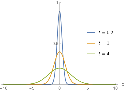
Figure 2: Gaussian distribution $d\mu_{X_{t}}\left(x\right)=\frac{1}{\sqrt{2\pi t}}e^{-x^{2}/2t}dx$, $t>0$ (variance).

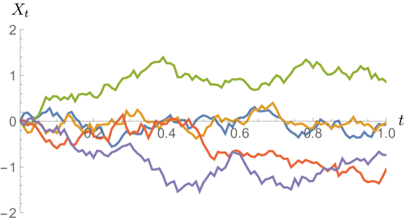
Figure 3: Monte-Carlo simulation of Brownian motion starting at $x=0$, with 5 sample paths. (“Monte-Carlo simulation” refers to the use of computer-generated random numbers.)

Let $G$ be a locally compact group, and let $\left(\Omega,\mathscr{F},\mathbb{P}\right)$ be a probability space, $\mathscr{F}$ a sigma-algebra, and $\mathbb{P}$ a probability measure defined on $\mathscr{F}$. A stochastic $L^{2}$-process is a system of random variables $\{X_{g}\}_{g\in G}$, $X_{g}\in L^{2}\left(\Omega,\mathscr{F},\mathbb{P}\right)$. The covariance function $c_{X}:G\times G\rightarrow\mathbb{C}$ of the process is given by

$$c_{X}\left(g_{1},g_{2}\right)=\mathbb{E}\left(\overline{X}_{g_{1}}X_{g_{2}}\right),\quad\forall\left(g_{1},g_{2}\right)\in G\times G.$$ (19)

To simplify, we will assume that the mean $\mathbb{E}\left(X_{g}\right)=\int_{\Omega}X_{g}d\mathbb{P}\left(\omega\right)=0$ for all $g\in G$.

We say that $\left(X_{g}\right)$ is stationary iff

$$c_{X}\left(hg_{1},hg_{2}\right)=c_{X}\left(g_{1},g_{2}\right),\quad\forall h\in G.$$ (20)

In this case $c_{X}$ is a function of $g_{1}^{-1}g_{2}$, i.e.,

$$\mathbb{E}\left(X_{g_{1}},X_{g_{2}}\right)=c_{X}\left(g_{1}^{-1}g_{2}\right),\quad\forall g_{1},g_{2}\in G;$$ (21)

(setting $h=g_{1}^{-1}$ in (20).)

The covariance function of Brownian motion $\mathbb{E}(X_{s}X_{t})$ is computed in Example 4.4 below.

4 Overview of Applications of RKHSs

In a general setup, reproducing kernel Hilbert spaces (RKHSs) were pioneered by Aronszajn in the 1950s Aro (50); and subsequently they have been used in a host of applications; e.g., SZ (09, 07).

The key idea of Aronszajn is that a RKHS is a Hilbert space $\mathscr{H}_{K}$ of functions $f$ on a set such that the values $f(x)$ are “reproduced” from $f$ and a vector $K_{x}$ in $\mathscr{H}_{K}$, in such a way that the inner product $\langle K_{x},K_{y}\rangle=:K\left(x,y\right)$ is a positive definite kernel.

Since this setting is too general for many applications, it is useful to restrict the very general framework for RKHSs to concrete cases in the study of particular spectral theoretic problems; p.d. functions on groups is a case in point. Such specific issues arise in physics (e.g., Fal (74); Jor (07)) where one is faced with extending p.d. functions $F$ which are only defined on a subset of a given group.

Connections to Gaussian Processes

By a theorem of Kolmogorov, every Hilbert space may be realized as a (Gaussian) reproducing kernel Hilbert space (RKHS), see e.g., PS (75); IM (65); SNFBK (10), and Theorem 4.2 below.

Definition 4.1.

A function $c$ defined on a subset of a group $G$ is said to be positive definite iff

$$\sum\nolimits_{i=1}^{n}\sum\nolimits_{j=1}^{n}\overline{\lambda_{i}}\lambda_{j}c\left(g_{i}^{-1}g_{j}\right)\geq 0$$ (22)

for all $n\in\mathbb{N}$, and all $\left\{\lambda_{i}\right\}_{i=1}^{n}\subset\mathbb{C}$, $\left\{g_{i}\right\}_{i=1}^{n}\subset G$ with $g_{i}^{-1}g_{j}$ in the domain of $c$.

From (22), it follows that $F\left(g^{-1}\right)=\overline{F\left(g\right)}$, and $\left|F\left(g\right)\right|\leq F\left(e\right)$, for all $g$ in the domain of $F$, where $e$ is the neutral element in $G$.

We recall the following theorem of Kolmogorov. One direction is easy, and the other is the deep part:

Theorem 4.2 (Kolmogorov).

A function $c:G\rightarrow\mathbb{C}$ is positive definite if and only if there is a stationary Gaussian process $\left(\Omega,\mathscr{F},\mathbb{P},X\right)$ with mean zero, such that $c=c_{X}$, i.e., $c\left(g_{1},g_{2}\right)=\mathbb{E}(\overline{X}_{g_{1}}X_{g_{2}})$; see (19).

Proof 4.3.

We refer to PS (75) for the non-trivial direction. To stress the idea, we include a proof of the easy part of the theorem:

Assume $c=c_{X}$. Let $\left\{\lambda_{i}\right\}_{i=1}^{n}\subset\mathbb{C}$ and $\left\{g_{i}\right\}_{i=1}^{n}\subset G$, then we have

$$\sum\nolimits_{i}\sum\nolimits_{j}\overline{\lambda_{i}}\lambda_{j}c\left(g_{i}^{-1}g_{j}\right)=\mathbb{E}\big{(}\big{|}\sum\lambda_{i}X_{g_{i}}\big{|}^{2}\big{)}\geq 0,$$

i.e., $c$ is positive definite.     ∎

Example 4.4.

Let $\Omega=\left[0,1\right]$, the closed unit interval, and let $\mathscr{H}:=$ the space of continuous functions $\xi$ on $\Omega$ such that $\xi\left(0\right)=0$, and $\xi^{\prime}\in L^{2}\left(0,1\right)$, where $\xi^{\prime}=\frac{d}{dx}\xi$ is the weak derivative of $\xi$, i.e., the derivative in the Schwartz-distribution sense. For $x,y\in\Omega$, set

$$\begin{split}K\left(x,y\right)&=x\wedge y=\min\left(x,y\right);\;\mbox{and}\\ K_{x}\left(y\right)&=K\left(x,y\right).\end{split}$$ (23)

Then in the sense of distribution, we have

$$\left(K_{x}\right)^{\prime}=\chi_{\left[0,x\right]};$$ (24)

i.e., the indicator function of the interval $\left[0,x\right]$, see Figure 4.

For $\xi_{1},\xi_{2}\in\mathscr{H}$, set

$$\left\langle\xi_{1},\xi_{2}\right\rangle_{\mathscr{H}}:=\int_{0}^{1}\overline{\xi_{1}^{\prime}\left(x\right)}\xi_{2}^{\prime}\left(x\right)dx.$$

Since $L^{2}\left(0,1\right)\subset L^{1}\left(0,1\right)$, and $\xi\left(0\right)=0$ for $\xi\in\mathscr{H}$, we see that

$$\xi\left(x\right)=\int_{0}^{x}\xi^{\prime}\left(y\right)dy,\quad\xi^{\prime}\in L^{2}\left(0,1\right),$$ (25)

and $\mathscr{H}$ consists of continuous functions on $\Omega$.

Claim 1.

The Hilbert space $\mathscr{H}$ is a RKHS with $\left\{K_{x}\right\}_{x\in\Omega}$ as its kernel; see (23).

Proof 4.5.

Let $\xi\in\mathscr{H}$, then by (25), we have:

$$\xi\left(x\right) =\int_{0}^{1}\chi_{\left[0,x\right]}\left(y\right)\xi^{\prime}\left(y\right)dy=\int_{0}^{1}K_{x}^{\prime}\left(y\right)\xi^{\prime}\left(y\right)dy$$

$$=\left\langle K_{x},\xi\right\rangle_{\mathscr{H}},\quad\forall x\in\Omega.$$

∎

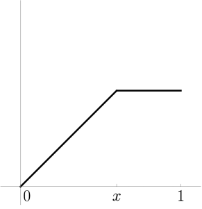
(a) $K_{x}\left(\cdot\right)$

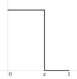
(b) $\chi_{\left[0,x\right]}\left(\cdot\right)$

Figure 4: $K_{x}$ and its distributional derivative.

Remark 4.6.

In the case of Example 4.4 above, the Gaussian process resulting from the p.d. kernel (23) is standard Brownian motion Hid (80), see Section 28. We shall return to the p.d. kernel (23) in Chapters 2, 4, and 6. It is the covariance kernel for standard Brownian motion in the interval $\left[0,1\right]$.

Subsequently, we shall be revisiting a number of specific instances of these RKHSs. Our use of them ranges from the most general case, when a continuous positive definite (p.d.) function $F$ is defined on an open subset of a locally compact group; the RKHS will be denoted $\mathscr{H}_{F}$. However, we stress that the associated RKHS will depend on both the function $F$, and on the subset of $G$ where $F$ is defined; hence on occasion, to be specific about the subset, we shall index the RKHS by the pair $\left(\Omega,F\right)$. If the choice of subset is implicit in the context, we shall write simply $\mathscr{H}_{F}$. Depending on the context, a particular RKHS typically will have any number of concrete, hands-on realizations, allowing us thereby to remove the otherwise obtuse abstraction entailed in its initial definition.

A glance at the Table of Contents indicates a large variety of the classes of groups, and locally defined p.d. functions we consider, and subsets. In each case, both the specific continuous, locally defined p.d. function considered, and its domain are important. Each of the separate cases has definite applications. The most explicit computations work best in the case when $G=\mathbb{R}$; and we offer a number of applications in three areas: applications to stochastic processes (Sections 20-29), to harmonic analysis (Sections 34-37), and to operator/spectral theory (Section 24).

5 Earlier Papers

Below we mention some earlier papers dealing with one or the other of the two extension problems (i) or (ii) in Section 1. To begin with, there is a rich literature on (i), and a little on (ii), but comparatively much less is known about their interconnections.

As for positive definite (p.d.) functions, their use and applications are extensive and includes such areas as stochastic processes, see e.g., JP13a ; AJSV (13); JP (12); AJ (12); harmonic analysis (see BCR (84); JÓ (00, 98), and the references there); potential theory Fug (74); KL (14); operators in Hilbert space ADL⁺ (10); Alp92a ; AD (86); JN (15); and spectral theory AH (13); Nus (75); Dev (72, 59). We stress that the literature is vast, and the above list is only a small sample.

Extensions of continuous p.d. functions defined on subsets of Lie groups $G$ was studied in Jor (91). In our present analysis of its connections to the extension questions for associated operators in Hilbert space, we will be making use of tools from spectral theory, and from the theory of reproducing kernel Hilbert spaces, such as can be found in e.g., Nel (69); Jør (81); ABDdS (93); Aro (50).

There is a different kind of notion of positivity involving reflections, restrictions, and extensions. It comes up in physics and in stochastic processes, and is somewhat related to our present theme. While they have several names, “reflection positivity” is a popular term. In broad terms, the issue is about realizing geometric reflections as “conjugations” in Hilbert space. When the program is successful, for a given unitary representation $U$ of a Lie group $G$, it is possible to renormalize the Hilbert space on which $U$ is acting.

Now the Bochner transform $F$ of a probability measure (e.g., the distribution of a stochastic process) which further satisfies reflection positivity, has two positivity properties: one (i) because $F$ is the transform of a positive measure, so $F$ is positive definite; and in addition the other, (ii) because of reflection symmetry (see the discussion after Corollary 8.20.) We have not followed up below with structural characterizations of this family of positive definite functions, but readers interested in the theme will find details in JÓ (00, 98); Arv (86); OS (73), and in the references given there.

To help readers to appreciate other approaches, as well as current research, we add below citation to some recent papers covering one or the other of the many aspects of the extension problem, which is the focus of our presentation here BT (11); BD (07); BT (07); KL (07); Sas (06); Bis (02).

6 Organization

We begin with a quick summary of preliminaries, making clear our setting and our choice of terminology. While we shall consider a host of variants of related extension questions for positive definite (p.d.) functions, the following theme is stressed in Chapter 2 below: Starting with a given and fixed, locally defined p.d. $F$ (say $F$ may be defined only in an open neighborhood in an ambient space), then consider first the naturally associated Hilbert space, arising from $F$ as a reproducing kernel Hilbert space (RKHS), $\mathscr{H}_{F}$. The question is then: When is it possible to realize an extension as a globally defined p.d. function $\widetilde{F}$, i.e., $\widetilde{F}$ extending $F$, in a construction which uses only spectral theory for operators in the initial RKHS, $\mathscr{H}_{F}$? And when will it be necessary to enlarge the initial Hilbert space, by passing to a dilation Hilbert space $\mathscr{K}$ containing an isometric copy of $\mathscr{H}_{F}$ itself?

The monograph is organized around the following themes, some involving dichotomies; e.g.,

1. Abelian (sect 12, ch 4-6) vs non-Abelian (sect 13);

2. simply connected (sect 18) vs connected (sect 17);

3. spectral theoretic (sect 12, 13, 35) vs geometric (sect 19);

4. extensions of p.d. functions vs extensions of systems of operators (sect 19); and

5. existence (ch 2) vs computation (ch 6-7) and classification (ch 10).

Item (1) refers to the group $G$ under consideration. In order to get started, we will need $G$ to be locally compact so it comes with Haar measure, but it may be non-Abelian. It may be a Lie group, or it may be non-locally Euclidean. In the other end of this dichotomy, we look at $G=\mathbb{R}$, the real line. In all cases, in the study of the themes from (1) it is important whether the group is simply connected or not.

In order to quickly get to concrete examples, we begin the real line $G=\mathbb{R}$ (Section 8.1), and $G=\mathbb{R}^{n}$, $n>1$ (Section 14); and the circle group, $G=\mathbb{T}=\mathbb{R}/\mathbb{Z}$ (Section 15).

Of the other groups, we offer a systematic treatment of the classes when $G$ is locally compact Abelian (Section 12), and the case of Lie groups (Section 13).

We note that the subdivision into classes of groups is necessary as the theorems we prove in the case of $G=\mathbb{R}$ have a lot more specificity than their counterparts do, for the more general classes of groups. One reason for this is that our harmonic analysis relies on unitary representations, and the non-commutative theory for unitary representations is much more subtle than is the Abelian counterpart.

Taking a choice of group $G$ as our starting point, we then study continuous p.d. functions $F$ defined on certain subsets in $G$. In the case of $G=\mathbb{R}$, our choice of subset will be a finite open interval centered at $x=0$.

Our next step is to introduce a reproducing kernel Hilbert space (RKHS) $\mathscr{H}_{F}$ that captures the properties of the given p.d. function $F$. The nature and the harmonic analysis of this particular RKHS are of independent interest; see Sections 4, 9, 14, and 24.

In Section 24, we study a certain trace class integral operator, called the Mercer operator. A Mercer operator $T_{F}$ is naturally associated to a given a continuous and p.d. function $F$ defined on the open interval, say $\left(-1,1\right)$. We use $T_{F}$ in order to identify natural Bessel frame in the corresponding RKHS $\mathscr{H}_{F}$. We then introduce a notion of Shannon sampling of finite Borel measures on $\mathbb{R}$, sampling from integer points in $\mathbb{R}$. In Corollary 25.5 we then use this to give a necessary and sufficient condition for a given finite Borel measure $\mu$ to fall in the convex set $Ext\left(F\right)$: The measures in $Ext\left(F\right)$ are precisely those whose Shannon sampling recover the given p.d. function $F$ on the interval $\left(-1,1\right)$.

In the general case for $G$, the questions we address are as follows:

1. What (if any) are the continuous p.d. functions on $G$ which extend $F$? (Sections 9, 18, and Chapters 5, 6.) Denoting the set of these extensions $Ext\left(F\right)$, then $Ext\left(F\right)$ is a compact convex set. Our next questions are:

2. What are the parameters for $Ext\left(F\right)$? (Section 18, Chapters 5 and 11.)

3. How can we understand $Ext\left(F\right)$ from a generally non-commutative extension problem for operators in $\mathscr{H}_{F}$? (See especially Section 24.)

4. We are further concerned with applications to scattering theory (e.g., Theorem 14.1), and to commutative and non-commutative harmonic analysis.

5. The unbounded operators we consider are defined naturally from given p.d. functions $F$, and they have a common dense domain in the RKHS $\mathscr{H}_{F}$. In studying possible selfadjoint operator extensions in $\mathscr{H}_{F}$ we make use of von Neumann’s theory of deficiency indices. For concrete cases, we must then find the deficiency indices; they must be equal, but whether they are $\left(0,0\right)$, $\left(1,1\right)$, $\left(d,d\right)$, $d>1$, is of great significance to the answers to the questions from (a)-(d).

6. Finally, what is the relevance of the solutions in (a) and (b) for the theory of operators in Hilbert space and their harmonic (and spectral) analysis? (Sections 14, 35, 36, and Chapter 11.)

Citations for (a)-(f) above.

1. Dev (59); JN (15); KW (82); Rud (63, 70).

2. JPT (13); Sch38b ; Pól (49); Nus (75); Jor (90, 91).

3. JM (84); JT14a ; Nel (59).

4. LP (89); JPT (15); Maa (10); JPT (12).

5. JPT (13); DS (88); Ion (01); KW (82); vN32a .

6. Sch (84, 85); JT14a ; Nel (57).

It is nice to know that the computer understands the problem. But I would like to understand it too. — Eugene Wigner

Chapter 2 Extensions of Continuous Positive Definite Functions

We begin with a study of a family of reproducing kernel Hilbert spaces (RKHSs) arising in connection with extension problems for positive definite (p.d.) functions. While the extension problems make sense, and are interesting, in a wider generality, we restrict attention here to the case of continuous p.d. functions defined on open subsets of groups $G$. We study two questions:

(i) When is a given partially defined continuous p.d. function extendable to the whole group $G$? In other words, when does it have continuous p.d. extensions to $G$?

(ii) When continuous p.d. extensions exist, what is the structure of all continuous p.d. extensions?

Because of available tools (mainly spectral theory for linear operators in Hilbert space), we restrict here our focus as follows: In the Abelian case, to when $G$ is locally compact; and if $G$ is non-Abelian, we assume that it is a Lie group. But our most detailed results are for the two cases $G=\mathbb{R}^{n}$, and $\mathbb{T}^{n}=\mathbb{R}^{n}/\mathbb{Z}^{n}$.

Historically, the cases $n=1$ and $n=2$ are by far the most studied, and they are also our main focus here. Available results are then much more explicit, and the applications perhaps more far reaching. Our results and examples for the case of $n=1$, we feel, are of independent interest; and they are motivated by such applications as harmonic analysis, sampling and interpolation theory, stochastic processes, and Lax-Phillips scattering theory. One reason for the special significance of the case $n=1$ is its connection to the theory of unbounded Hermitian linear operators with prescribed dense domain in Hilbert space, and their extensions. Indeed, if $n=1$, the possible continuous p.d. extensions of given partially defined p.d. function $F$ are connected with associated extensions of certain unbounded Hermitian linear operators; in fact two types of such extensions: In one case, there are selfadjoint extensions in the initial RKHS (Type I); and in another case, the selfadjoint extensions necessarily must be realized in an enlargement Hilbert space (Type II); so in a Hilbert space properly bigger than the initial RKHS associated to $F$.

7 The RKHS $\mathscr{H}_{F}$

In our theorems and proofs, we shall make use of reproducing kernel Hilbert spaces (RKHSs), but the particular RKHSs we need here will have additional properties (as compared to a general framework); which allow us to give explicit formulas for our solutions.

Our present setting is more restrictive in two ways: (i) we study groups $G$, and translation-invariant kernels, and (ii) we further impose continuity. By “translation” we mean relative to the operation in the particular group under discussion. Our presentation below begins with the special case when $G$ is the circle group $\mathbb{T}=\mathbb{R}/\mathbb{Z}$, or the real line $\mathbb{R}$.

For simplicity we focus on the case $G=\mathbb{R}$, indicating the changes needed for $G=\mathbb{T}$. Modifications, if any, necessitated by considering other groups $G$ will be described in the body of the book.

Lemma 7.1.

Let $\Omega$ be open subset of $\mathbb{R}^{n}$, and let $F$ be a continuous function, defined on $\Omega-\Omega$; then $F$ is positive definite (p.d.) if and only if the following holds:

$$\int_{\Omega}\int_{\Omega}\overline{\varphi(x)}\varphi(y)F(x-y)dxdy\geq 0,\quad\forall\varphi\in C_{c}^{\infty}(\Omega).$$

Proof 7.2.

Standard.     ∎

Consider a continuous p.d. function $F:\Omega-\Omega\rightarrow\mathbb{C}$, and set

$$F_{y}\left(x\right):=F\left(x-y\right),\quad\forall x,y\in\Omega.$$ (26)

Let $\mathscr{H}_{F}$ be the reproducing kernel Hilbert space (RKHS), which is the completion of

$$\left\{\sum\nolimits_{\text{finite}}c_{j}F_{x_{j}}\>\big{|}\ x_{j}\in\Omega,\>c_{j}\in\mathbb{C}\right\}$$ (27)

with respect to the inner product

$$\left\langle\sum\nolimits_{i}c_{i}F_{x_{i}},\sum\nolimits_{j}d_{j}F_{y_{j}}\right\rangle_{\mathscr{H}_{F}}:=\sum\nolimits_{i}\sum\nolimits_{j}\overline{c_{i}}d_{j}F\left(x_{i}-y_{j}\right);$$ (28)

modulo the subspace of functions with zero $\left\|\cdot\right\|_{\mathscr{H}_{F}}$-norm.

Remark 7.3.

Throughout, we use the convention that the inner product is conjugate linear in the first variable, and linear in the second variable. When more than one inner product is used, subscripts will make reference to the Hilbert space.

Lemma 7.4.

The RKHS, $\mathscr{H}_{F}$, is the Hilbert completion of the functions

$$F_{\varphi}\left(x\right)=\int_{\Omega}\varphi\left(y\right)F\left(x-y\right)dy,\quad\forall\varphi\in C_{c}^{\infty}\left(\Omega\right),\;x\in\Omega$$ (29)

with respect to the inner product

$$\left\langle F_{\varphi},F_{\psi}\right\rangle_{\mathscr{H}_{F}}=\int_{\Omega}\int_{\Omega}\overline{\varphi\left(x\right)}\psi\left(y\right)F\left(x-y\right)dxdy,\quad\forall\varphi,\psi\in C_{c}^{\infty}\left(\Omega\right).$$ (30)

In particular,

$$\left\|F_{\varphi}\right\|_{\mathscr{H}_{F}}^{2}=\int_{\Omega}\int_{\Omega}\overline{\varphi\left(x\right)}\varphi\left(y\right)F\left(x-y\right)dxdy.$$ (31)

Proof 7.5.

Indeed, setting $\varphi_{n,x}\left(t\right):=n\varphi\left(n\left(t-x\right)\right)$ (see Lemma 7.6), we have

$$\left\|F_{\varphi_{n,x}}-F_{x}\right\|_{\mathscr{H}_{F}}\rightarrow 0,\;\mbox{as }n\rightarrow\infty.$$ (32)

Hence $\left\{F_{\varphi}\right\}_{\varphi\in C_{c}^{\infty}\left(\Omega\right)}$ spans a dense subspace in $\mathscr{H}_{F}$. For more details, see Jor (86, 87, 90).

Lemma 7.6.

For $\Omega=\left(\alpha,\beta\right)$, let $a=\beta-\alpha$. Let $\alpha<x<\beta$ and let $\varphi_{n,x}\left(t\right)=n\varphi\left(n\left(t-x\right)\right)$, where $\varphi$ satisfies

1. $\mathrm{supp}\left(\varphi\right)\subset\left(-a,a\right)$;

2. $\varphi\in C_{c}^{\infty}$, $\varphi\geq 0$;

3. $\int\varphi\left(t\right)dt=1$. Note that $\lim_{n\rightarrow\infty}\varphi_{n,x}=\delta_{x}$, the Dirac measure at $x$.

Then

$$\lim_{n\rightarrow\infty}\left\|F_{\varphi_{n,x}}-F_{x}\right\|_{\mathscr{H}_{F}}=0$$ (33)

Hence $\left\{F_{\varphi}\>|\>\varphi\in C_{c}^{\infty}\left(\Omega\right)\right\}$ spans a dense subspace in $\mathscr{H}_{F}$.

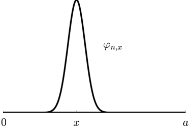
Figure 5: The approximate identity $\varphi_{n,x}\left(\cdot\right)$

The facts below about $\mathscr{H}_{F}$ follow from the general theory of RKHS Aro (50):

• For $F$ continuous, p.d., and non zero, $F(0)>0$, so we can always arrange $F(0)=1.$

• $F(-x)=\overline{F(x)}$, $\left|F\left(x\right)\right|\leq F\left(0\right)$

• $\mathscr{H}_{F}$ consists of continuous functions $\xi:\Omega\rightarrow\mathbb{C}$.

• The reproducing property holds:

  $$\left\langle F_{x},\xi\right\rangle_{\mathscr{H}_{F}}=\xi\left(x\right),\quad\forall\xi\in\mathscr{H}_{F},\>\forall x\in\Omega.$$

  This is a direct consequence of the definition of $\mathscr{H}_{F}$, see (28).

• If $F_{\phi_{n}}\to\xi$ in $\mathscr{H}_{F}$, then $F_{\phi_{n}}$ converges uniformly to $\xi$ in $\Omega$. In fact, the reproducing property yields the estimate:

  $$\left|F_{\phi_{n}}\left(x\right)-\xi\left(x\right)\right| =\left|\left\langle F_{x},F_{\phi_{n}}-\xi\right\rangle_{\mathscr{H}_{F}}\right|$$

  $$\leq\left\|F_{x}\right\|_{\mathscr{H}_{F}}\left\|F_{\phi_{n}}-\xi\right\|_{\mathscr{H}_{F}}$$

  $$=F\left(0\right)^{1/2}\left\|F_{\phi_{n}}-\xi\right\|_{\mathscr{H}_{F}}\xrightarrow{\;n\rightarrow\infty\;}0.$$

Theorem 7.7.

A continuous function $\xi:\Omega\rightarrow\mathbb{C}$ is in $\mathscr{H}_{F}$ if and only if there exists $A_{0}>0$, such that

$$\sum\nolimits_{i}\sum\nolimits_{j}\overline{c_{i}}c_{j}\overline{\xi\left(x_{i}\right)}\xi\left(x_{j}\right)\leq A_{0}\sum\nolimits_{i}\sum\nolimits_{j}\overline{c_{i}}c_{j}F\left(x_{i}-x_{j}\right)$$ (34)

for all finite system $\left\{c_{i}\right\}\subset\mathbb{C}$ and $\left\{x_{i}\right\}\subset\Omega$.

Equivalently, for all $\psi\in C_{c}^{\infty}\left(\Omega\right)$,

$$\left|\int_{\Omega}\psi\left(y\right)\xi\left(y\right)dy\right|^{2} \leq A_{0}\int_{\Omega}\int_{\Omega}\overline{\psi\left(x\right)}\psi\left(y\right)F\left(x-y\right)dxdy.$$ (35)

Proof 7.8.

It suffices to check condition (35).

If (35) holds, then $F_{\psi}\mapsto\int_{\Omega}\overline{\xi\left(x\right)}\psi\left(x\right)dx$ is a bounded linear functional on the dense subspace $\left\{F_{\psi}\>|\>\psi\in C_{c}^{\infty}\left(\Omega\right)\right\}$ in $\mathscr{H}_{F}$ (Lemma 7.6), hence it extends to $\mathscr{H}_{F}$. Therefore, $\exists!\>l_{\xi}\in\mathscr{H}_{F}$ s.t.

$$\int_{\Omega}\overline{\xi\left(x\right)}\psi\left(x\right)dx \overset{\left(\text{Riesz}\right)}{=} \left\langle l_{\xi},F_{\psi}\right\rangle_{\mathscr{H}_{F}}$$

$$\overset{\left(\text{Fubini}\right)}{=} \int_{\Omega}\psi\left(y\right)\left\langle l_{\xi},F_{y}\right\rangle_{\mathscr{H}_{F}}dy$$

$$= \int_{\Omega}\overline{l_{\xi}\left(y\right)}\psi\left(y\right)dy,\quad\forall\psi\in C_{c}^{\infty}\left(\Omega\right);$$

and this implies $\xi=l_{\xi}\in\mathscr{H}_{F}$.

Conversely, assume $\xi\in\mathscr{H}_{F}$ then $\left|\langle\xi,F_{\psi}\rangle_{\mathscr{H}_{F}}\right|^{2}\leq\|\xi\|_{\mathscr{H}_{F}}^{2}\|F_{\psi}\|_{\mathscr{H}_{F}}^{2}$, for all $\psi\in C_{c}^{\infty}\left(\Omega\right)$. Thus (35) follows.     ∎

These two conditions (34)($\Longleftrightarrow$(35)) are the best way to characterize elements in the Hilbert space $\mathscr{H}_{F}$; see also Corollary 7.10.

We will be using this when considering for example the deficiency-subspaces for skew-symmetric operators with dense domain in $\mathscr{H}_{F}$.

Example 7.9.

Let $G=\mathbb{T}=\mathbb{R}/\mathbb{Z}$, e.g., represented as $\left(-\frac{1}{2},\frac{1}{2}\right]$. Fix $0<a<\frac{1}{2}$, then $\Omega-\Omega=\left(-a,a\right)$ mod $\mathbb{Z}$. So, for example, (1) takes the form $F:(-a,a)\text{ mod }\mathbb{Z}\to\mathbb{C}$. See Figure 6.

Figure 6: Two versions of $\Omega=\left(0,a\right)\subset\mathbb{T}^{1}$.

An Isometry

It is natural to extend the mapping from (29) to measures, i.e., extending

$$C_{c}^{\infty}\left(\Omega\right)\ni\varphi\longmapsto F_{\varphi}\in\mathscr{H}_{F}\left(\mbox{the RKHS}\right),$$

by replacing $\varphi$ with a Borel measure $\mu$ on $\Omega$. Specifically, set:

$$\left(S\mu\right)\left(x\right)=F_{\mu}\left(x\right):=\int_{\Omega}F\left(x-y\right)d\mu\left(y\right).$$ (36)

Then the following result follows from the discussion above.

Corollary 7.10.

1. Let $\mu$ be a Borel measure on $\Omega$ (possibly a signed measure), then the following two conditions are equivalent:

   $$\int_{\Omega}\int_{\Omega} F\left(x-y\right)\overline{d\mu\left(x\right)}d\mu\left(y\right)<\infty;$$ (37)

   $$\Updownarrow$$

   $$S\mu \in\mathscr{H}_{F}\;\left(\text{see $\left(\ref{eq:tu1}\right)$}.\right)$$ (38)

2. If the conditions hold, then

   $$\int_{\Omega}\int_{\Omega}F\left(x-y\right)d\mu\left(x\right)d\mu\left(y\right)=\left\|S\mu\right\|_{\mathscr{H}_{F}}^{2}$$ (39)

   (where the norm on the r.h.s. in (39) is the RKHS-norm.)

3. And moreover, for all $\xi\in\mathscr{H}_{F}$, we have

   $$\left\langle\xi,S\mu\right\rangle_{\mathscr{H}_{F}}=\int_{\Omega}\overline{\xi\left(x\right)}d\mu\left(x\right).$$ (40)

4. In particular, we note that all the Dirac measures $\mu=\delta_{x}$, for $x\in\Omega$, satisfy (37), and that

   $$S\left(\delta_{x}\right)=F\left(\cdot-x\right)\in\mathscr{H}_{F}.$$ (41)

5. For every $x,y\in\Omega$, we have

   $$\left\langle\delta_{x},\delta_{y}\right\rangle_{\mathfrak{M}_{2}\left(\Omega,F\right)}=F\left(x-y\right),$$ (42)

   where the r.h.s. in (42) refers to the $\mathfrak{M}_{2}$-Hilbert inner product.

In other words, the signed measures $\mu$ satisfying (37) form a Hilbert space $\mathfrak{M}_{2}\left(\Omega,F\right)$, and $S$ in (36) defines an isometry of $\mathfrak{M}_{2}\left(\Omega,F\right)$ onto the RKHS $\mathscr{H}_{F}$. Here $\mathfrak{M_{2}}\left(\Omega,F\right)$ denotes the Hilbert space determined by condition (37) above.

Example 7.11.

$G=\mathbb{R}$, $a>0$, $\Omega=\left(0,a\right)$,

$$F\left(x\right)=e^{-\left|x\right|},\quad\left|x\right|<a.$$ (43)

We now apply the isometry $S:\mathfrak{M}_{2}\left(F\right)\xrightarrow{\;\simeq\;}\mathscr{H}_{F}$ (onto) to this example. The two functions

$$\xi_{+}\left(x\right)=e^{-x},\;\mbox{and }\xi_{-}\left(x\right)=e^{x-a},\;x\in\Omega,$$

will play an important role (defect-vectors) in Chapter 4 below. We have

$$S^{*}\xi_{+} = \delta_{0}\in\mathfrak{M}_{2}\left(F\right),\;\mbox{and}$$ (44)

$$S^{*}\xi_{-} = \delta_{a}\in\mathfrak{M}_{2}\left(F\right),$$ (45)

where $\delta_{0}$ and $\delta_{a}$ denote the respective Dirac measures. The proof of (44)-(45) is immediate from Corollary 7.10.

Corollary 7.12.

Let $F$ and $\Omega$ be as above; and assume further that $F$ is $C^{\infty}$, then

$$F^{\left(n\right)}\left(\cdot-x\right)\in\mathscr{H}_{F},\quad\mbox{for all }x\in\Omega.$$ (46)

Proof 7.13.

We may establish (46) by induction, starting with the first derivative.

Let $x\in\Omega$; then for sufficiently small $h$, $\left|h\right|<\varepsilon$, we have $F\left(\cdot-x-h\right)\in\mathscr{H}_{F}$; and moreover,

$$\left\|\frac{F\left(\cdot-x-h\right)-F\left(\cdot-x\right)}{h}\right\|_{\mathscr{H}_{F}}^{2} = \frac{1}{h^{2}}\left(F\left(0\right)+F\left(0\right)-2F\left(-h\right)\right)$$

$$= \frac{1}{h}\left(\frac{F\left(0\right)-F\left(-h\right)}{h}-\frac{F\left(-h\right)-F\left(0\right)}{h}\right)$$

$$\rightarrow -F^{\left(2\right)}\left(0\right),\;\mbox{as}\;h\rightarrow 0.$$

Hence, the limit of the difference quotient on the r.h.s. in (7.13) exists relative to the norm in $\mathscr{H}_{F}$, and so the limit $-F^{\prime}\left(\cdot-x\right)$ is in $\mathscr{H}_{F}$.     ∎

We further get the following:

Corollary 7.14.

If $F$ is p.d. and $C^{2}$ in a neighborhood of $0$, then $F^{\left(2\right)}\left(0\right)\leq 0$.

Remark 7.15.

Note that, for $\xi\in\mathscr{H}_{F}$, (38) is an integral equation, i.e.,

$$\xi\left(x\right)=\int_{\Omega}F\left(x-y\right)d\nu\left(y\right);\;\mbox{solving for }\nu\in\mathfrak{M}_{2}\left(F\right).$$ (48)

Using Corollary 7.12, we note that, when p.d. $F\in C^{\infty}\left(\Omega-\Omega\right)$, then (48) also has distribution solutions $\nu$.

8 The Skew-Hermitian Operator $D^{(F)}$ in $\mathscr{H}_{F}$

In our discussion of the operator $D^{\left(F\right)}$ (Definition 8.2), we shall make use of von Neumann’s theory of symmetric (or skew-symmetric) linear operators with dense domain in a fixed Hilbert space; see e.g., vN32a ; LP (85); Kre (46); JLW (69); dBR (66); DS (88).

The general setting is as follows: Let $\mathscr{H}$ be a complex Hilbert space, and let $\mathscr{D}\subset\mathscr{H}$ be a dense linear subspace. A linear operator $D$, defined on $\mathscr{D}$, is said to be skew-symmetric iff (Def)

$$\left\langle Df,g\right\rangle_{\mathscr{H}}+\left\langle f,Dg\right\rangle_{\mathscr{H}}=0$$ (49)

holds for all $f,g\in\mathscr{D}$. If we introduce the adjoint operator $D^{*}$, then (49) is equivalent to the following containment of graphs:

$$D\subseteq-D^{*}.$$ (50)

As in the setting of von Neumann, the domain of $D^{*}$, $dom(D^{*})$, is as follows:

$$dom(D^{*}) = \Big{\{}g\in\mathscr{H}\>|\>\exists\>\mbox{const}\>C=C_{g}<\infty\;\mbox{s.t.}\;$$ (51)

$$\left|\left\langle g,Df\right\rangle_{\mathscr{H}}\right|\leq C\left\|f\right\|_{\mathscr{H}},\;\forall f\in\mathscr{D}\Big{\}}.$$

And the vector $D^{*}g$ satisfies

$$\left\langle D^{*}g,f\right\rangle_{\mathscr{H}}=\left\langle g,Df\right\rangle_{\mathscr{H}}$$ (52)

for all $f\in\mathscr{D}$.

An extension $A$ of $D$ is said to be skew-adjoint iff (Def)

$$A=-A^{*};$$ (53)

which is “$=$”, not merely containment, comparing (50).

We are interested in skew-adjoint extensions, since the Spectral Theorem applies to them; not to the operators which are merely skew-symmetric; see DS (88). From the Spectral Theorem, we then get solutions to our original extension problem for locally defined p.d. functions.

But, in the general Hilbert space setting, skew-adjoint extensions need not exist. However we have the following:

Theorem 8.1 (von Neumann DS (88)).

A skew-symmetric operator $D$ has skew-adjoint extensions $A$, i.e.,

$$D\subseteq A\subseteq-D^{*}$$ (54)

if and only if the following two subspaces of $\mathscr{H}$ (deficiency spaces, see Definition 8.7) have equal dimension:

$$DEF{}^{\pm}\left(D\right)=\mathscr{N}\left(D^{*}\pm I\right),$$

i.e., $\dim DEF{}^{+}\left(D\right)=\dim DEF{}^{-}\left(D\right)$, where

$$DEF{}^{\pm}\left(D\right)=\left\{g_{\pm}\in dom(D^{*})\;|\;D^{*}g_{\pm}=\mp g_{\pm}\right\}.$$

Below, we introduce $D^{\left(F\right)}$ systematically and illustrate how to use the corresponding skew-adjoint extensions to extend locally defined p.d. functions.

Fix a continuous p.d. function $F:\Omega-\Omega\rightarrow\mathbb{C}$, where $\Omega=(0,a)$, a finite open interval in $\mathbb{R}$. Let $\mathscr{H}_{F}$ be the corresponding RKHS.

Definition 8.2.

Set

$$dom(D^{\left(F\right)})=\left\{F_{\psi}\>|\>\psi\in C_{c}^{\infty}\left(\Omega\right)\right\},\;\mbox{and}$$

$$D^{\left(F\right)}F_{\psi}=F_{\psi^{\prime}},\quad\forall F_{\psi}\in dom(D^{\left(F\right)}),$$

where $\psi^{\prime}\left(x\right)=d\psi/dx$, and $F_{\psi}$ is as in (29).

Note that the recipe for $D^{\left(F\right)}$ yields a well-defined operator with dense domain in $\mathscr{H}_{F}$. To see this, use Schwarz’ lemma to show that if $F_{\psi}=0$ in $\mathscr{H}_{F}$, then it follows that the vector $F_{\psi^{\prime}}\in\mathscr{H}_{F}$ is 0 as well. An alternative proof is given in Lemma 8.5.

Lemma 8.3.

The operator $D^{\left(F\right)}$ is skew-symmetric and densely defined in $\mathscr{H}_{F}$.

Proof 8.4.

By Lemma 7.4 $dom(D^{(F)})$ is dense in $\mathscr{H}_{F}.$ If $\psi\in C_{c}^{\infty}\left(0,a\right)$ and $\left|t\right|<\mathrm{dist}\left(\mathrm{supp}\left(\psi\right),\mbox{endpoints}\right)$, then

$$\left\|F_{\psi\left(\cdot+t\right)}\right\|_{\mathscr{H}_{F}}^{2}=\left\|F_{\psi}\right\|_{\mathscr{H}_{F}}^{2}=\int_{0}^{a}\int_{0}^{a}\overline{\psi\left(x\right)}\psi\left(y\right)F\left(x-y\right)dxdy$$ (55)

by (31). Thus,

$$\frac{d}{dt}\left\|F_{\psi\left(\cdot+t\right)}\right\|_{\mathscr{H}_{F}}^{2}=0$$

which is equivalent to

$$\langle D^{\left(F\right)}F_{\psi},F_{\psi}\rangle_{\mathscr{H}_{F}}+\langle F_{\psi},D^{\left(F\right)}F_{\psi}\rangle_{\mathscr{H}_{F}}=0.$$ (56)

It follows that $D^{\left(F\right)}$ is skew-symmetric.

Lemma 8.5 below shows that $D^{\left(F\right)}$ is well-defined on its dense domain in $\mathscr{H}_{F}$. This finishes the proof of Lemma 8.3.     ∎

Lemma 8.5.

The following implication holds:

$$\left[\psi\in C_{c}^{\infty}\left(\Omega\right),\>F_{\psi}=0\mbox{ in }\mathscr{H}_{F}\right]$$ (57)

$$\Downarrow$$

$$\left[F_{\psi^{\prime}}=0\mbox{ in }\mathscr{H}_{F}\right]$$ (58)

Proof 8.6.

Substituting (57) into

$$\left\langle F_{\varphi},F_{\psi^{\prime}}\right\rangle_{\mathscr{H}_{F}}+\left\langle F_{\varphi^{\prime}},F_{\psi}\right\rangle_{\mathscr{H}_{F}}=0$$

we get

$$\left\langle F_{\varphi},F_{\psi^{\prime}}\right\rangle_{\mathscr{H}_{F}}=0,\quad\forall\varphi\in C_{c}^{\infty}\left(\Omega\right).$$

Taking $\varphi=\psi^{\prime}$, yields

$$\left\langle F_{\psi^{\prime}},F_{\psi^{\prime}}\right\rangle=\bigl{\|}F_{\psi^{\prime}}\bigr{\|}_{\mathscr{H}_{F}}^{2}=0$$

which is the desired conclusion (58). Therefore, the operator $D^{\left(F\right)}$ is well-defined.     ∎

Definition 8.7.

Let $(D^{\left(F\right)})^{*}$ be the adjoint of $D^{\left(F\right)}$. The deficiency spaces $DEF^{\pm}$ consists of $\xi_{\pm}\in\mathscr{H}_{F}$, such that $(D^{\left(F\right)})^{*}\xi_{\pm}=\pm\xi_{\pm}$. That is,

$$DEF^{\pm}=\left\{\xi_{\pm}\in\mathscr{H}_{F}:\left\langle F_{\psi^{\prime}},\xi_{\pm}\right\rangle_{\mathscr{H}_{F}}=\left\langle F_{\psi},\pm\xi_{\pm}\right\rangle_{\mathscr{H}_{F}},\;\forall\psi\in C_{c}^{\infty}\left(\Omega\right)\right\}.$$

Elements in $DEF^{\pm}$ are called defect vectors. The dimensions of $DEF^{\pm}$, i.e., the pair of numbers

$$d_{\pm}=\dim DEF^{\pm},$$

are called the deficiency indices of $D^{\left(F\right)}$. See, e.g., vN32a ; Kre (46); DS (88); AG (93); Nel (69). Example 7.11 above is an instance of deficiency indices $\left(1,1\right)$, i.e., $d_{+}=d_{-}=1$.

von Neumann showed that a densely defined Hermitian operator in a Hilbert space has equal deficiency indices if it commutes with a conjugation operator DS (88). This criterion is adapted to our setting in Lemma 8.8 and its corollary.

The Case of Conjugations

The purpose of the section below is to show that, for a large class of locally defined p.d. functions $F$, it is possible to establish existence of skew-adjoint extensions of the corresponding operator $D^{\left(F\right)}$ with the use of a criterion of von Neumann: It states that, if a skew-Hermitian operator anti-commutes with a conjugation (a conjugate linear period-2 operator), then it must have equal deficiency indices, and therefore have skew-adjoint extensions. In the present case, the anti-commuting properties takes the form of (60) below.

Lemma 8.8.

Let $\Omega=(\alpha,\beta).$ Suppose $F$ is a real-valued p.d. function defined on $\Omega-\Omega$. The operator $J$ on $\mathscr{H}_{F}$ determined by

$$JF_{\varphi}=\overline{F_{\varphi(\alpha+\beta-x)}},\quad\varphi\in C_{c}^{\infty}\left(\Omega\right)$$

is a conjugation, i.e., $J$ is conjugate-linear, $J^{2}$ is the identity operator, and

$$\left\langle JF_{\phi},JF_{\psi}\right\rangle_{\mathscr{H}_{F}}=\left\langle F_{\psi},F_{\phi,}\right\rangle_{\mathscr{H}_{F}}.$$ (59)

Moreover,

$$D^{\left(F\right)}J=-JD^{\left(F\right)}.$$ (60)

Proof 8.9.

Let $a:=\alpha+\beta$ and $\phi\in C_{c}^{\infty}(\Omega).$ Since $F$ is real-valued, we have

$$JF_{\phi}(x) =\int_{\alpha}^{\beta}\overline{\phi(a-y)}\,\overline{F(x-y)}dy$$

$$=\int_{\alpha}^{\beta}\psi(y)\,F(x-y)dy$$

where $\psi(y):=\overline{\phi(a-y)}$ is in $C_{c}^{\infty}(\Omega)$. It follows that $J$ maps the the operator domain $dom(D^{(F)})$ onto itself. For $\phi,\psi\in C_{c}^{\infty}(\Omega)$,

$$\left\langle JF_{\phi},F_{\psi}\right\rangle_{\mathscr{H}_{F}} =\int_{\alpha}^{\beta}F_{\phi(a-\cdot)}(x)\psi(x)dx$$

$$=\int_{\alpha}^{\beta}\int_{\alpha}^{\beta}\phi(a-y)F(x-y)\psi(x)dydx.$$

Making the change of variables $(x,y)\to(a-x,a-y)$ and interchanging the order of integration we see that

$$\left\langle JF_{\phi},F_{\psi}\right\rangle_{\mathscr{H}_{F}} =\int_{\alpha}^{\beta}\int_{\alpha}^{\beta}\phi(y)F(y-x)\psi(a-x)dydx$$

$$=\int_{\alpha}^{\beta}\phi(y)F_{\psi(a-\cdot)}(y)dy$$

$$=\left\langle JF_{\psi},F_{\phi}\right\rangle_{\mathscr{H}_{F}},$$

establishing (59).

Finally, for all $\phi\in C_{c}^{\infty}(\Omega)$,

$$JD^{(F)}F_{\phi}=\overline{F_{\phi^{\prime}(a-\cdot)}}=-\overline{F_{\tfrac{d}{dx}\left(\phi\left(a-\cdot\right)\right)}}=-D^{(F)}JF_{\phi},$$

hence (60) holds.     ∎

Corollary 8.10.

If $F$ is real-valued, then $DEF^{+}$ and $DEF^{-}$ have the same dimension.

Proof 8.11.

This follows from Lemma 8.8, see e.g, AG (93) or DS (88).     ∎

We proceed to characterize the deficiency spaces of $D^{\left(F\right)}$.

Lemma 8.12.

If $\xi\in DEF^{\pm}$ then $\xi(y)=\mathrm{constant}\,e^{\mp y}.$

Proof 8.13.

Specifically, $\xi\in DEF^{+}$ if and only if

$$\int_{0}^{a}\psi^{\prime}\left(y\right)\xi\left(y\right)dy=\int_{0}^{a}\psi\left(y\right)\xi\left(y\right)dy,\quad\forall\psi\in C_{c}^{\infty}\left(0,a\right).$$

Equivalently, $y\mapsto\xi\left(y\right)$ is a weak solution to the ODE $\xi^{\prime}=-\xi$, i.e., a strong solution in $C^{1}$. Thus, $\xi\left(y\right)=\mbox{constant }e^{-y}$. The $DEF^{-}$ case is similar.     ∎

Corollary 8.14.

Suppose $F$ is real-valued. Let $\xi_{\pm}(y):=e^{\mp y},$ for $y\in\Omega.$ Then $\xi_{+}\in\mathscr{H}_{F}$ iff $\xi_{-}\in\mathscr{H}_{F}.$ In the affirmative case $\left\|\xi_{-}\right\|_{\mathscr{H}_{F}}=e^{a}\left\|\xi_{+}\right\|_{\mathscr{H}_{F}}.$

Proof 8.15.

Let $J$ be the conjugation from Lemma 8.8. A short calculation:

$$\left\langle J\xi,F_{\phi}\right\rangle_{\mathscr{H_{F}}} =\left\langle F_{\overline{\phi(a-\cdot)}},\xi\right\rangle_{\mathscr{H_{F}}}=\int\phi(a-x)\xi(x)dx$$

$$=\int\phi(x)\xi(a-x)dx=\left\langle\overline{\xi(a-\cdot)},F_{\phi}\right\rangle_{\mathscr{H_{F}}}$$

shows that $\left(J\xi\right)(x)=\overline{\xi(a-x)}$, for $\xi\in\mathscr{H}_{F}$. In particular, $J\xi_{-}=e^{a}\xi_{+}$. Since $\left\|J\xi_{-}\right\|_{\mathscr{H}_{F}}=\left\|\xi_{-}\right\|_{\mathscr{H}_{F}}$, the proof is easily completed.     ∎

Corollary 8.16.

The deficiency indices of $D^{\left(F\right)}$, with its dense domain in $\mathscr{H}_{F}$, are $\left(0,0\right)$, $(0,1),$ $(1,0),$ or $\left(1,1\right)$.

The second case in the above corollary happens precisely when $y\mapsto e^{-y}\in\mathscr{H}_{F}$. We can decide this with the use of (34)($\Leftrightarrow$(35)).

In Chapter 8 we will give some a priori estimates, which enable us to strengthen Corollary 8.16. For this, see Corollary 33.28.

Remark 8.17.

Note that deficiency indices $\left(1,1\right)$ is equivalent to

$$\sum\nolimits_{i}\sum\nolimits_{j}\overline{c_{i}}c_{j}e^{-\left(x_{i}+x_{j}\right)} \leq A_{0}\sum\nolimits_{i}\sum\nolimits_{j}\overline{c_{i}}c_{j}F\left(x_{i}-x_{j}\right)$$ (61)

$$\Updownarrow$$

$$\left|\int_{0}^{a}\psi\left(y\right)e^{-y}dy\right|^{2} \leq A_{0}\int_{0}^{a}\int_{0}^{a}\overline{\psi\left(x\right)}\psi\left(y\right)F\left(x-y\right)dxdy$$

But it depends on $F$ (given on $\left(-a,a\right)$).

Lemma 8.18.

On $\mathbb{R}\times\mathbb{R}$, define the following kernel $K_{+}\left(x,y\right)=e^{-\left|x+y\right|}$, $\left(x,y\right)\in\mathbb{R}\times\mathbb{R}$; then this is a positive definite kernel on $\mathbb{R}_{+}\times\mathbb{R}_{+}$; (see Aro (50) for details on positive definite kernels.)

Proof 8.19.

Let $\{c_{j}\}\subset\mathbb{C}^{N}$ be a finite system of numbers, and let $\left\{x_{j}\right\}\subset\mathbb{R}_{+}^{N}$. Then

$$\sum\nolimits_{j}\sum\nolimits_{k}\overline{c_{j}}c_{k}e^{-\left(x_{j}+x_{k}\right)}=\left|\sum\nolimits_{j}c_{j}e^{-x_{j}}\right|^{2}\geq 0.$$

∎

Corollary 8.20.

Let $F$, $\mathscr{H}_{F}$, and $D^{\left(F\right)}$ be as in Corollary 8.16; then $D^{\left(F\right)}$ has deficiency indices $\left(1,1\right)$ if and only if the kernel $K_{+}\left(x,y\right)=e^{-\left|x+y\right|}$ is dominated by $K_{F}\left(x,y\right):=F\left(x-y\right)$ on $\left(0,a\right)\times\left(0,a\right)$, i.e., there is a finite positive constant $A_{0}$ such that

$$A_{0}K_{F}-K_{+}$$

is positive definite on $\left(0,a\right)\times\left(0,a\right)$.

Proof 8.21.

This is immediate from the lemma and (61) above.     ∎

In a general setting the kernels with the properties from Corollary 8.20 are called reflection positive kernels. See Example 8.22, and Section 18. Their structure is accounted for by Theorem 31.5. Their applications includes the study of Gaussian processes, the theory of unitary representations of Lie groups, and quantum fields. The following references give a glimpse into this area of analysis, JÓ (98, 00); Kle (74). See also the papers and books cited there.

Example 8.22.

The following are examples of positive definite functions on $\mathbb{R}$ which are used in a variety of applications. We discuss in Section 28 how they arise as extensions of locally defined p.d. functions, and some of the applications. In the list below, $F:\mathbb{R}\rightarrow\mathbb{R}$ is p.d., and $a,b>0$ are fixed constants.

1. ${\displaystyle F\left(x\right)=e^{-a\left|x\right|}}$; Sections 17 (p.17), 18 (p.18), 28 (p.28).

2. ${\displaystyle F\left(x\right)=\frac{1-e^{-b\left|x\right|}}{b\left|x\right|}}$

3. ${\displaystyle F\left(x\right)=\frac{1}{1+\left|x\right|}}$

4. ${\displaystyle F\left(x\right)=\frac{1}{\sqrt{1+\left|x\right|}}e^{-\frac{\left|x\right|}{1+\left|x\right|}}}$

These are known to be generators of Gaussian reflection positive processes JÓ (98, 00); Kle (74), i.e., having completely monotone covariance functions. For details of these functions, see Theorem 31.5 (the Bernstein-Widder Theorem). The only one among these which is also a Markov process is the one coming from $F\left(x\right)=e^{-a\left|x\right|}$, $x\in\mathbb{R}$, where $a>0$ is a parameter; it is the Ornstein-Uhlenbeck process. Note that $F\left(x\right)=e^{-\left|x\right|}$, $x\in\mathbb{R}$, induces the positive definite kernel in Lemma 8.18, i.e., $K_{+}\left(x,y\right)=e^{-\left(x+y\right)}$, $\left(x,y\right)\in\mathbb{R}_{+}\times\mathbb{R}_{+}$.

For these reasons Example (1) in the above list shall receive relatively more attention than the other three. Another reason for Example (1) playing a prominent role is that almost all the central questions dealing with locally defined p.d. functions are especially transparent for this example.

More generally, a given p.d. function $F$ on $\mathbb{R}$ is said to be reflection positive if the induced kernel on $\mathbb{R}_{+}\times\mathbb{R}_{+}$, given by

$$K_{+}\left(x,y\right)=F\left(x+y\right),\quad\left(x,y\right)\in\mathbb{R}_{+}\times\mathbb{R}_{+},$$

is positive definite.

In the case of a given p.d. function $F$ on $\mathbb{R}^{n}$, the reflection positivity making reference to some convex cone $C_{+}$ in $\mathbb{R}^{n}$, and we say that $F$ is $C_{+}$-reflection positive if

$$K_{+}\left(x,y\right):=F\left(x+y\right),\quad\left(x,y\right)\in C_{+}\times C_{+},$$

is a positive definite kernel (on $C_{+}\times C_{+}$.)

Example 8.23.

Let $\Omega=\left(-1,1\right)$ be the interval $-1<x<1$. The following consideration illustrates the difference between positive definite (p.d.) kernels and positive definite functions:

1. On $\Omega\times\Omega$, set $K\left(x,y\right):={\displaystyle\frac{1}{1-xy}}$.

2. On $\Omega$, set $F\left(x\right):={\displaystyle\frac{1}{1-x^{2}}}$.

Then $K$ is a p.d. kernel, but $F$ is not a p.d. function.

It is well known that $K$ is a p.d. kernel. The RKHS of $K$ consists of analytic functions $\xi\left(x\right)=\sum_{n=0}^{\infty}c_{n}x^{n}$, $\left|x\right|<1$, such that $\sum_{n=0}^{\infty}\left|c_{n}\right|^{2}<\infty$. In fact,

$$\left\|\xi\right\|_{\mathscr{H}_{K}}^{2}=\sum_{n=0}^{\infty}\left|c_{n}\right|^{2}.$$

To see that $F$ is not a p.d. function, one checks that the $2\times 2$ matrix

$$\begin{pmatrix}F\left(0\right)&F\left(x\right)\\ F\left(-x\right)&F\left(0\right)\end{pmatrix}=\begin{pmatrix}1&\frac{1}{1-x^{2}}\\ \frac{1}{1-x^{2}}&1\end{pmatrix}$$

has a negative eigenvalue $\lambda\left(x\right)=\frac{-x^{2}}{1-x^{2}}$, when $x\in\Omega\backslash\left\{0\right\}$.

The following theorem, an inversion formula (see (62)), shows how the full domain, $-\infty<x<\infty$, of a continuous positive definite function $F$ is needed in determining the positive Borel measure $\mu$ which yields the Bochner-inversion, i.e., $F=\widehat{d\mu}$.

Theorem 8.24 (An inversion formula (see e.g., Akh (65); LP (89); DM (76))).

Let $F$ be a continuous positive definite function on $\mathbb{R}$ such that $F\left(0\right)=1$. Let $\mu$ be the Borel probability measure s.t. $F=\widehat{d\mu}$ (from Bochner’s theorem), and let $\left(a_{0},b_{0}\right)$ be a finite open interval, with the two-point set $\left\{a_{0},b_{0}\right\}$ of endpoints. Then

$$\mu\left(\left(a_{0},b_{0}\right)\right)+\frac{1}{2}\left(\left\{a_{0},b_{0}\right\}\right)=\frac{1}{2\pi}\lim_{T\rightarrow\infty}\int_{-T}^{T}\frac{e^{-ixa_{0}}-e^{-ixb_{0}}}{ix}F\left(x\right)dx.$$ (62)

(The second term on the l.h.s. in (62) is $\left(\mu\left(\left\{a_{0}\right\}\right)+\mu\left(\left\{b_{0}\right\}\right)\right)/2$.)

Proof 8.25.

The proof details are left to the reader. They are straightforward, and also contained in many textbooks on harmonic analysis.     ∎

Remark 8.26.

Suppose $F$ is continuous and positive definite, but is only known on a finite centered interval $\left(-a,a\right)$, $a>0$. Formula (62) now shows how distinct positive definite extensions $\widetilde{F}$ (to $\mathbb{R}$) for $F$ (on $\left(-a,a\right)$) yields distinct measures $\mu_{\widetilde{F}}$. However, a measure $\mu$ cannot be determined (in general) from $F$ alone, i.e., from $x$ in a finite interval $\left(-a,a\right)$.

8.1 Illustration: $G=\mathbb{R}$, correspondence between the two extension problems

Extensions of continuous p.d. functions vs extensions of operators. Illustration for the case of $\left(-a,a\right)\subset\mathbb{R}$, i.e., given $F:\left(-a,a\right)\rightarrow\mathbb{C}$, continuous and positive definite:

We illustrate how to use the correspondence

$$\boxed{\mbox{extensions of p.d. functions}}\longleftrightarrow\boxed{\mbox{extensions of operators}}$$

to get from $F\left(t\right)$ on $\left|t\right|<a$ to $\widetilde{F}\left(t\right)$, $t\in\mathbb{R}$, with $\widetilde{F}=\widehat{d\mu}$.

Figure 7 illustrates the extension correspondence (p.d. function vs extension operator) in the case of Type I, but each step in the correspondence carries over to the Type II case. The main difference is that for Type II, one must pass to a dilation Hilbert space, i.e., a larger Hilbert space containing $\mathscr{H}_{F}$ as an isometric copy.

Notations:

1. $\left\{U\left(t\right)\right\}_{t\in\mathbb{R}}$: unitary one-parameter group with generator $A^{\left(F\right)}\supset D^{\left(F\right)}$

2. $P_{U}\left(\cdot\right)=$ the corresponding projection-valued measure (PVM)

3. $U\left(t\right)=\int_{\mathbb{R}}e^{it\lambda}P_{U}\left(d\lambda\right)$

4. $d\mu\left(x\right)=\left\|P_{U}\left(dx\right)F_{0}\right\|_{\mathscr{H}_{F}}^{2}$

5. An extension: $\widetilde{F}\left(t\right)=\widehat{d\mu}=\int_{\mathbb{R}}e^{itx}d\mu\left(x\right)=\left\langle F_{0},U\left(t\right)F_{0}\right\rangle_{\mathscr{H}_{F}}$

Figure 7: Extension correspondence. From locally defined p.d $F$ to $D^{\left(F\right)}$, to a skew-adjoint extension, and the unitary one-parameter group, to spectral resolution, and finally to an associated element in $Ext(F)$.

For the more general non-commutative correspondence (extension of p.d. vs operator extension), we refer to Section 13.1, the GNS-construction. Compare with Figure 10.

Next, we flesh out in detail the role of $D^{\left(F\right)}$ in extending a given p.d. function $F$, defined on $\Omega-\Omega$. This will be continued in Section 9 in a more general setting.

By Corollary 8.16, we conclude that there exists skew-adjoint extension $A^{\left(F\right)}\supset D^{\left(F\right)}$ in $\mathscr{H}_{F}$. That is, $dom(D^{\left(F\right)})\subset dom(A^{\left(F\right)})\subset\mathscr{H}_{F}$, $(A^{\left(F\right)})^{*}=-A^{\left(F\right)}$, and

$$D^{\left(F\right)}=A^{\left(F\right)}\Big{|}_{dom(D^{\left(F\right)})}.$$

Given a skew-adjoint extension $A^{\left(F\right)}\supset D^{\left(F\right)}$, set $U\left(t\right)=e^{tA^{\left(F\right)}}:\mathscr{H}_{F}\rightarrow\mathscr{H}_{F}$, and get the unitary one-parameter group

$$\left\{U\left(t\right):t\in\mathbb{R}\right\},\;U\left(s+t\right)=U\left(s\right)U\left(t\right),\;\forall s,t\in\mathbb{R};$$

and if

$$\xi\in dom(A^{\left(F\right)})=\left\{\xi\in\mathscr{H}_{F}\>|\>s.t.-\lim_{t\rightarrow 0}\frac{U\left(t\right)\xi-\xi}{t}\>\mbox{exists}\right\}$$

then

$$A^{\left(F\right)}\xi=\lim_{t\rightarrow 0}\frac{U\left(t\right)\xi-\xi}{t}.$$ (63)

Now let

$$\widetilde{F}_{A}\left(t\right):=\left\langle F_{0},U\left(t\right)F_{0}\right\rangle_{\mathscr{H}_{F}},\quad\forall t\in\mathbb{R}.$$ (64)

Using (33), we see that $\widetilde{F}_{A}\left(t\right)$, defined on $\mathbb{R}$, is a continuous p.d. extension of $F$.

Lemma 8.27.

$\widetilde{F}_{A}\left(t\right)$ as in (64) is a continuous bounded p.d. function of $\mathbb{R}$, and

$$\widetilde{F}_{A}\left(t\right)=F\left(t\right),\quad t\in\left(-a,a\right).$$ (65)

Proof 8.28.

Since $\left\{U\left(t\right)\right\}$ is a strongly continuous unitary group acting on $\mathscr{H}_{F}$, we have

$$\left|\widetilde{F}_{A}\left(t\right)\right|=\left|\left\langle F_{0},U\left(t\right)F_{0}\right\rangle\right|\leq\left\|F_{0}\right\|_{\mathscr{H}_{F}}\left\|U\left(t\right)F_{0}\right\|_{\mathscr{H}_{F}}=\left\|F_{0}\right\|_{\mathscr{H}_{F}}^{2}=F\left(0\right),$$

by (28). Recall that $F_{x}=F\left(\cdot-x\right)$, $x\in\Omega=\left(0,a\right)$. This shows that every $F^{ext}$ is bounded and continuous.

The proof that $\widetilde{F}_{A}\left(t\right)$ indeed extends $F$ to $\mathbb{R}$ holds in a more general context, see e.g., Theorem 9.1 and Jor (89, 90, 91).     ∎

Recall that $F$ can always be normalized by $F\left(0\right)=1$. Consider the spectral representation:

$$U\left(t\right)=e^{tA^{\left(F\right)}}=\int_{-\infty}^{\infty}e^{i\lambda t}P\left(d\lambda\right)$$ (66)

where $P\left(\cdot\right)$ is the projection-valued measure of $A^{\left(F\right)}$. Thus, $P\left(B\right):\mathscr{H}_{F}\rightarrow\mathscr{H}_{F}$ is a projection, for all Borel subsets $B$ in $\mathbb{R}$. Setting

$$d\mu\left(\lambda\right)=\left\|P\left(d\lambda\right)F_{0}\right\|_{\mathscr{H}_{F}}^{2}$$ (67)

then the corresponding extension is as follows:

$$\widetilde{F}_{A}\left(t\right)=\int_{-\infty}^{\infty}e^{i\lambda t}d\mu\left(\lambda\right)=\widehat{d\mu}\left(t\right),\quad\forall t\in\mathbb{R}.$$ (68)

Conclusion. The extension $\widetilde{F}_{A}\left(t\right)$ from (64) has nice transform properties, and via (68) we get

$$\mathscr{H}_{\widetilde{F}_{A}}\simeq L^{2}\left(\mathbb{R},\mu\right)$$

with the transformation $T_{\mu}$ of Theorem 9.1; where $\mathscr{H}_{\widetilde{F}_{A}}$ is the RKHS of the extended p.d. function $\widetilde{F}_{A}$. The explicit transform $T_{\mu}$ realizing $\mathscr{H}_{F}\xrightarrow{\;\simeq\;}L^{2}\left(\mu\right)$ is given in Corollary 12.15.

Corollary 8.29.

Let a partially defined p.d. function $F$ be given as in Figure 7. Let $D^{\left(F\right)}$ be the associated skew-Hermitian operator in $\mathscr{H}_{F}$, and assume that it has a skew-adjoint extension $A$. Let $P_{A}\left(\cdot\right)$ and $\mu_{A}\left(\cdot\right)$ be the measures from (66) and (67), then $\widetilde{F}_{A}=\widehat{d\mu_{A}}$ is a Type I extension, and

$$suppt\left(\mu_{A}\right)=i\cdot spect\left(A\right),\quad i=\sqrt{-1}.$$

Proof 8.30.

Immediate from the proof of Lemma 8.27.     ∎

Remark 8.31.

In the circle case $G=\mathbb{T}$, the extension $\widetilde{F}_{A}$ in (64) needs not be $\mathbb{Z}$-periodic.

Consider $a>0$, $\Omega=\left(0,a\right)$, and a continuous p.d. function $F$ on $\left(-a,a\right)$. Let $D^{\left(F\right)}$ be the corresponding skew-Hermitian operator in $\mathscr{H}_{F}$. We proved that for every skew-adjoint extension $A\supset D^{\left(F\right)}$ in $\mathscr{H}_{F}$, the corresponding p.d. function

$$F_{A}\left(t\right)=\left\langle F_{0},e^{tA}F_{0}\right\rangle_{\mathscr{H}_{F}}=\int_{\mathbb{R}}e^{it\lambda}\left\|P_{A}\left(d\lambda\right)F_{0}\right\|_{\mathscr{H}_{F}}^{2},\quad t\in\mathbb{R}$$ (69)

is a Type I p.d. extension of $F$; see formulas (67)-(68).

Proposition 8.32.

Let $F$ be continuous and p.d. on $\left(-a,a\right)$; and let $\widetilde{F}$ be a Type I positive definite extension to $\mathbb{R}$, i.e.,

$$F\left(t\right)=\widetilde{F}\left(t\right),\quad\forall t\in\left(-a,a\right).$$ (70)

Then there is a skew-adjoint extension $A$ of $D^{\left(F\right)}$ such that $\widetilde{F}=F_{A}$ on $\mathbb{R}$; see (69) above.

Proof 8.33.

By the definition of Type I, we know that there is a strongly continuous unitary one-parameter group $\{U\left(t\right)\}_{t\in\mathbb{R}}$, acting in $\mathscr{H}_{F}$; such that

$$F\left(t\right)=\left\langle F_{0},U\left(t\right)F_{0}\right\rangle_{\mathscr{H}_{F}},\quad\forall t,\;\left|t\right|<a.$$ (71)

By Stone’s Theorem, there is a unique skew-adjoint operator $A$ in $\mathscr{H}_{F}$ such that $U\left(t\right)=e^{tA}$, $\forall t\in\mathbb{R}$; and so the r.h.s. is $F_{A}=\widetilde{F}$; i.e., the given Type I extension $\widetilde{F}$ has the form $F_{A}$. But differentiation, $d/dt$ at $t=0$, in (71) shows that $A$ is an extension of $D^{\left(F\right)}$ which is the desired conclusion.     ∎

9 Enlarging the Hilbert Space

The purpose of this section is to describe the dilation-Hilbert space in detail, and to prove some lemmas which will then be used in Chapter 5. In Chapter 5, we identify extensions of the initial positive definite (p.d.) function $F$ which are associated with operator extensions in $\mathscr{H}_{F}$ (Type I), and those which require an enlargement of $\mathscr{H}_{F}$ (Type II).

To simplify notations, results in this section are formulated for $G=\mathbb{R}$. The modification for general Lie groups is straightforward, and are left for the reader.

Fix $a>0$, and $\Omega=\left(0,a\right)\subset\mathbb{R}$. Let $F:\Omega-\Omega\to\mathbb{C}$ be a continuous p.d. function. Recall the corresponding reproducing kernel Hilbert space (RKHS) $\mathscr{H}_{F}$ is the completion of $span\left\{F_{x}:=F\left(\cdot-x\right)\>|\>x\in\Omega\right\}$ with respect to the inner product

$$\left\langle F_{x},F_{y}\right\rangle_{\mathscr{H}_{F}}:=F_{y}\left(x\right)=F\left(x-y\right),\quad\forall x,y\in\Omega,$$ (72)

modulo elements of zero $\mathscr{H}_{F}$-norm.

Following Section 7, let $F_{\varphi}=\varphi*F$ be the convolution, where

$$F_{\varphi}\left(x\right)=\int_{\Omega}\varphi\left(y\right)F\left(x-y\right)dy,\quad x\in\Omega,\;\varphi\in C_{c}^{\infty}\left(\Omega\right).$$

Setting

$$\pi\left(\varphi\right)F_{0}=F_{\varphi},\;\mbox{and}\;\varphi^{\#}\left(x\right)=\overline{\varphi\left(-x\right)},$$

we may write

$$\left\langle F_{\varphi},F_{\psi}\right\rangle_{\mathscr{H}_{F}}=\left\langle F_{0},\pi\left(\varphi^{\#}*\psi\right)F_{0}\right\rangle_{\mathscr{H}_{F}}=\left\langle\pi\left(\varphi\right)F_{0},\pi\left(\psi\right)F_{0}\right\rangle_{\mathscr{H}_{F}}.$$ (73)

The following theorem also holds in $\mathbb{R}^{n}$ with $n>1$. It is stated here for $n=1$ to illustrate the “enlargement” of $\mathscr{H}_{F}$ question.

Theorem 9.1.

The following two conditions are equivalent:

1. $F$ is extendable to a continuous p.d. function $\widetilde{F}$ defined on $\mathbb{R}$, i.e., $\widetilde{F}$ is a continuous p.d. function defined on $\mathbb{R}$ and $F\left(x\right)=\widetilde{F}\left(x\right)$ for all $x$ in $\Omega-\Omega$.

2. There is a Hilbert space $\mathscr{K}$, an isometry $W:\mathscr{H}_{F}\to\mathscr{K}$, and a strongly continuous unitary group $U_{t}:\mathscr{K}\to\mathscr{K}$, $t\in\mathbb{R}$, such that if $A$ is the skew-adjoint generator of $U_{t}$, i.e.,

   $$\lim_{t\rightarrow 0}\dfrac{1}{t}\left(U_{t}k-k\right)=Ak,\quad\forall k\in dom\left(A\right);$$ (74)

   then $\forall\varphi\in C_{c}^{\infty}\left(\Omega\right)$, we have

   $$WF_{\varphi}\in dom\left(A\right),\quad\mbox{and}$$ (75)

   $$AWF_{\varphi}=WF_{\varphi^{\prime}}.$$ (76)

The rest of this section is devoted to the proof of Theorem 9.1.

Lemma 9.2.

Let $W,\mathscr{H}_{F},\mathscr{K}$ and $U_{t}$ be as in the theorem. If $s,t\in\Omega$, and $\varphi\in C_{c}^{\infty}\left(\Omega\right)$, then

$$U_{t}WF_{\varphi}=WF_{\varphi_{t}},\;\mbox{and}$$ (77)

$$\left\langle WF_{\varphi},U_{t}WF_{\varphi}\right\rangle_{\mathscr{K}}=\left\langle F_{0},\pi\left(\varphi^{\#}*\varphi_{t}\right)F_{0}\right\rangle_{\mathscr{H}_{F}},$$ (78)

where $\varphi_{t}\left(\cdot\right)=\varphi\left(\cdot+t\right)$.

Proof 9.3.

We first establish (77). Consider

$$U_{t-s}WF_{\varphi_{s}}=\begin{cases}U_{t}WF_{\varphi}&\text{at }s=0\\ WF_{\varphi_{t}}&\text{at }s=t\end{cases}$$ (79)

and

$$\int_{0}^{t}\tfrac{d}{ds}\left(U_{t-s}WF_{\varphi_{s}}\right)ds=WF_{\varphi_{t}}-U_{t}WF_{\varphi}.$$ (80)

Note that the left-side of (80) equals zero. Indeed, (74) and (75) imply that

$$\tfrac{d}{ds}\left(U_{t-s}WF_{\varphi_{s}}\right)=-U_{t-s}AWF_{\varphi_{s}}+U_{t-s}WF_{\varphi_{s}^{\prime}}.$$

But (76) applied to $\varphi_{s}$ yields

$$AWF_{\varphi_{s}}=WF_{\varphi_{s}^{\prime}},$$ (81)

and so (80) is identically zero. The desired conclusion (77) follows.

Moreover, we have

$$l.h.s.\left(\ref{eq:e.6}\right) \overset{\text{by $\left(\ref{eq:e.9}\right)$}}{=} \left\langle WF_{\varphi},WF_{\varphi_{t}}\right\rangle_{\mathscr{K}}$$

$$\overset{\text{$W$ is isom.}}{=} \left\langle F_{\varphi},F_{\varphi_{t}}\right\rangle_{\mathscr{H}_{F}}$$

$$\overset{\text{by $\left(\ref{eq:e.1.1}\right)$}}{=} \left\langle F_{0},\pi\left(\varphi^{\#}*\varphi_{t}\right)F_{0}\right\rangle_{\mathscr{H}_{F}}$$

$$= r.h.s.\left(\ref{eq:e.6}\right).$$

∎

Proof 9.4.

(The proof of Theorem 9.1)

(2)$\Longrightarrow$(1) Assume there exist $\mathscr{K}$, $W$, $U_{t}$ and $A$ as in (2). Let

$$\widetilde{F}(t)=\left\langle WF_{0},U_{t}WF_{0}\right\rangle,\quad t\in\mathbb{R}.$$ (82)

By the Spectral Theorem, $U_{t}=\int_{\mathbb{R}}e^{i\lambda t}P\left(d\lambda\right)$, where $P\left(\cdot\right)$ is the corresponding projection-valued measure. Setting

$$d\mu\left(\lambda\right):=\left\|P\left(d\lambda\right)WF_{0}\right\|_{\mathscr{K}}^{2}=\left\langle WF_{0},P\left(d\lambda\right)WF_{0}\right\rangle_{\mathscr{K}},$$

then $\widetilde{F}=\widehat{d\mu}$, i.e., $\widetilde{F}$ is the Bochner transform of the Borel measure $d\mu$ on $\mathbb{R}$.

Let $\phi^{\left(\epsilon\right)}$, $\epsilon>0$, be an approximate identity at $x=0$. (That is, $\phi^{\left(\epsilon\right)}\rightarrow\delta_{0}$, as $\epsilon\rightarrow 0^{+}$; see Lemma 7.6 for details.) Then

$$\widetilde{F}\left(t\right) = \left\langle WF_{0},U_{t}WF_{0}\right\rangle_{\mathscr{K}}$$ (83)

$$= \lim_{\epsilon\to 0^{+}}\left\langle WF_{0},U_{t}WF_{\phi^{\left(\epsilon\right)}}\right\rangle_{\mathscr{K}}$$

$$\overset{\text{by $\left(\ref{eq:e.9}\right)$}}{=} \lim_{\epsilon\to 0^{+}}\left\langle WF_{0},WF_{\phi_{t}^{\left(\epsilon\right)}}\right\rangle_{\mathscr{K}}$$

$$= \lim_{\epsilon\to 0^{+}}\left\langle F_{0},F_{\phi_{t}^{\left(\epsilon\right)}}\right\rangle_{\mathscr{H}_{F}}$$

$$= \left\langle F_{0},F_{-t}\right\rangle_{\mathscr{H}_{F}}\overset{\text{by $\left(\ref{eq:e.1}\right)$}}{=}F\left(t\right),\quad t\in\Omega-\Omega;$$

Therefore, $\widetilde{F}$ is a continuous p.d. extension of $F$ to $\mathbb{R}$.

(1)$\Longrightarrow$(2) Let $\widetilde{F}=\widehat{d\mu}$ be a p.d. extension and Bochner transform. Define $W:\mathscr{H}_{F}\to\mathscr{H}_{\widetilde{F}}$, by

$$WF_{\varphi}=\widetilde{F}_{\varphi},\quad\varphi\in C_{c}^{\infty}\left(\Omega\right).$$ (84)

Then $W$ is an isometry and $\mathscr{H}_{\widetilde{F}}\backsimeq L^{2}(\mu)$. Indeed, for all $\varphi\in C_{c}^{\infty}(\Omega)$, since $\widetilde{F}$ is an extension of $F$, we have

$$\left\|F_{\varphi}\right\|_{\mathscr{H}_{F}}^{2} = \int_{\Omega}\int_{\Omega}\overline{\varphi\left(s\right)}\varphi\left(t\right)F\left(s-t\right)dsdt$$

$$= \int_{\mathbb{R}}\int_{\mathbb{R}}\overline{\varphi\left(s\right)}\varphi\left(t\right)\widetilde{F}\left(s-t\right)dsdt$$

$$= \int_{\mathbb{R}}\int_{\mathbb{R}}\overline{\varphi\left(s\right)}\varphi\left(t\right)\left(\int_{-\infty}^{\infty}e^{i\lambda\left(s-t\right)}d\mu\left(\lambda\right)\right)dsdt$$

$$\overset{\left(\text{Fubini}\right)}{=} \int_{\mathbb{R}}\left|\widehat{\varphi}\left(\lambda\right)\right|^{2}d\mu\left(\lambda\right)=\|\widetilde{F}_{\varphi}\|{}_{\mathscr{H}_{\widetilde{F}}}^{2}.$$

Now let

$$L^{2}\left(\mu\right)\ni f\xrightarrow{\quad U_{t}\quad}e^{i\lambda t}f\left(\lambda\right)\in L^{2}\left(\mu\right)$$

be the unitary group acting in $\mathscr{H}_{\widetilde{F}}\backsimeq L^{2}(\mu)$, and let $A$ be its generator. Then,

$$\left(WF_{\varphi}\right)\left(x\right)=\int_{\mathbb{R}}e^{i\lambda x}\widehat{\varphi}\left(\lambda\right)d\mu\left(\lambda\right),\quad\forall x\in\Omega,\>\forall\varphi\in C_{c}^{\infty}\left(\Omega\right);$$ (85)

and it follows that

$$\left(WF_{\varphi^{\prime}}\right)\left(x\right) = \int_{\mathbb{R}}e^{i\lambda x}i\lambda\widehat{\varphi}\left(\lambda\right)d\mu\left(\lambda\right)$$

$$= \frac{d}{dt}\Big{|}_{t=0}\left(U_{t}WF_{\varphi}\right)\left(x\right)=\left(AWF_{\varphi}\right)\left(x\right)$$

as claimed. This proves part (2) of the theorem.     ∎

An early instance of dilations (i.e., enlarging the Hilbert space) is the theorem by Sz.-Nagy RSN (56); Muh (74) on unitary dilations of strongly continuous semigroups.

We mention this result here to stress that p.d. functions on $\mathbb{R}$ (and subsets of $\mathbb{R}$) often arise from contraction semigroups.

Theorem 9.5 (Sz.-Nagy).

Let $\left\{S_{t}\>|\>t\in\mathbb{R}_{+}\right\}$ be a strongly continuous semigroup of contractive operator in a Hilbert space $\mathscr{H}$; then there is

1. a Hilbert space $\mathscr{K}$,

2. an isometry $V:\mathscr{H}\rightarrow\mathscr{K}$,

3. a strongly continuous one-parameter unitary group $\left\{U\left(t\right)\>|\>t\in\mathbb{R}\right\}$ acting on $\mathscr{K}$ such that

   $$VS_{t}=U\left(t\right)V,\quad\forall t\in\mathbb{R}_{+}$$ (86)

Sz.-Nagy also proved the following:

Theorem 9.6 (Sz.-Nagy).

Let $\left(S_{t},\mathscr{H}\right)$ be a contraction semigroup, $t\geq 0$, (such that $S_{0}=I_{\mathscr{H}}$;) and let $f_{0}\in\mathscr{H}\backslash\left\{0\right\}$; then the following function $F$ on $\mathbb{R}$ is positive definite:

$$F\left(t\right)=\begin{cases}\left\langle f_{0},S_{t}f_{0}\right\rangle_{\mathscr{H}}&\mbox{if }t\geq 0,\\ \left\langle f_{0},S_{-t}^{*}f_{0}\right\rangle_{\mathscr{H}}&\mbox{if }t<0.\end{cases}$$ (87)

Corollary 9.7.

Every p.d. function as in (87) has the form:

$$F\left(t\right):=\left\langle k_{0},U\left(t\right)k_{0}\right\rangle_{\mathscr{K}},\quad t\in\mathbb{R}$$ (88)

where $\left(U\left(t\right),\mathscr{K}\right)$ is a unitary representation of $\mathbb{R}$.

10 $Ext_{1}(F)$ and $Ext_{2}(F)$

Let $G$ be a locally compact group, and $\Omega$ an open connected subset of $G$. Consider a continuous p.d. function $F:\Omega^{-1}\cdot\Omega\rightarrow\mathbb{C}$.

We shall study the two sets of extensions in the title of this section.

Definition 10.1.

We say that $\left(U,\mathscr{K},k_{0}\right)\in Ext\left(F\right)$ iff

1. $U$ is a strongly continuous unitary representation of $G$ in the Hilbert space $\mathscr{K}$, containing the RKHS $\mathscr{H}_{F}$; and

2. there exists $k_{0}\in\mathscr{K}$ such that

   $$F\left(g\right)=\left\langle k_{0},U\left(g\right)k_{0}\right\rangle_{\mathscr{K}},\quad\forall g\in\Omega^{-1}\cdot\Omega.$$ (89)

Definition 10.2.

Let $Ext_{1}\left(F\right)\subset Ext\left(F\right)$ consisting of $\left(U,\mathscr{H}_{F},F_{e}\right)$ with

$$F\left(g\right)=\left\langle F_{e},U\left(g\right)F_{e}\right\rangle_{\mathscr{H}_{F}},\quad\forall g\in\Omega^{-1}\cdot\Omega;$$ (90)

where $F_{e}\in\mathscr{H}_{F}$ satisfies $\left\langle F_{e},\xi\right\rangle_{\mathscr{H}_{F}}=\xi\left(e\right)$, $\forall\xi\in\mathscr{H}_{F}$, and $e$ denotes the neutral (unit) element in $G$, i.e., $e\,g=g$, $\forall g\in G$.

Definition 10.3.

Let $Ext_{2}\left(F\right):=Ext\left(F\right)\backslash Ext_{1}\left(F\right)$, consisting of the solutions to problem (89) for which $\mathscr{K}\supsetneqq\mathscr{H}_{F}$, i.e., unitary representations realized in an enlargement Hilbert space.

Remark 10.4.

When $G=\mathbb{R}^{n}$, and $\Omega\subset\mathbb{R}^{n}$ is open and connected, we consider continuous p.d. functions $F:\Omega-\Omega\rightarrow\mathbb{C}$. In this special case, we have

$$Ext\left(F\right)= \Bigl{\{}\mu\in\mathscr{M}_{+}\left(\mathbb{R}^{n}\right)\>\big{|}\>\widehat{\mu}\left(x\right)=\int_{\mathbb{R}^{n}}e^{i\lambda\cdot x}d\mu\left(\lambda\right)$$ (91)

$$\mbox{ is a p.d. extensiont of $F$}\Bigr{\}}.$$

Note that (91) is consistent with (89). In fact, if $\left(U,\mathscr{K},k_{0}\right)$ is a unitary representation of $G=\mathbb{R}^{n}$, such that (89) holds; then, by a theorem of Stone, there is a projection-valued measure (PVM) $P_{U}\left(\cdot\right)$, defined on the Borel subsets of $\mathbb{R}^{n}$ s.t.

$$U\left(x\right)=\int_{\mathbb{R}^{n}}e^{i\lambda\cdot x}P_{U}\left(d\lambda\right),\quad x\in\mathbb{R}^{n}.$$ (92)

Setting

$$d\mu\left(\lambda\right):=\left\|P_{U}\left(d\lambda\right)k_{0}\right\|_{\mathscr{K}}^{2},$$ (93)

it is then immediate that $\mu\in\mathscr{M}_{+}\left(\mathbb{R}^{n}\right)$, and the finite measure $\mu$ satisfies

$$\widehat{\mu}\left(x\right)=F\left(x\right),\quad\forall x\in\Omega-\Omega.$$ (94)

The Case of $n=1$

Fix $a>0$, and $\Omega=\left(0,a\right)\subset\mathbb{R}$. Start with a local continuous p.d. function $F:\Omega-\Omega\rightarrow\mathbb{C}$, and let $\mathscr{H}_{F}$ be the corresponding RKHS. Let $Ext(F)$ be the compact convex set of probability measures on $\mathbb{R}$ defining extensions of $F$; see (91).

We see in Section 9 that all continuous p.d. extensions of $F$ come from strongly continuous unitary representations. So in the case of 1D, from unitary one-parameter groups of course, say $U(t)$. Further recall that some of the p.d. extensions of $F$ may entail a bigger Hilbert space, say $\mathscr{K}$. By this we mean that $\mathscr{K}$ creates a dilation (enlargement) of $\mathscr{H}_{F}$ in the sense that $\mathscr{H}_{F}$ is isometrically embedded in $\mathscr{K}$. Via the embedding we may therefore view $\mathscr{H}_{F}$ as a closed subspace in $\mathscr{K}$.

We now divide $Ext(F)$ into two parts, say $Ext_{1}(F)$ and $Ext_{2}(F)$. $Ext_{1}(F)$ is the subset of $Ext(F)$ corresponding to extensions when the unitary representation $U(t)$ acts in $\mathscr{H}_{F}$ (internal extensions), and $Ext_{2}(F)$ is the part of $Ext(F)$ associated to unitary representations $U(t)$ acting in a proper enlargement Hilbert space $\mathscr{K}$ (if any), i.e., acting in a Hilbert space $\mathscr{K}$ corresponding to a proper dilation. For example, the Pólya extensions in Chapter 5 account for a part of $Ext_{2}(F)$.

Now consider the canonical skew-Hermitian operator $D^{\left(F\right)}$ in the RKHS $\mathscr{H}_{F}$ (Definition 8.2), i.e.,

$$D^{\left(F\right)}\left(F_{\varphi}\right)=F_{\varphi^{\prime}}\quad\mbox{where}$$ (95)

$$F_{\varphi}\left(x\right)=\int_{\Omega}\varphi\left(y\right)F\left(x-y\right)dy,\quad\varphi\in C_{c}^{\infty}\left(\Omega\right).$$ (96)

As shown in Section 7, $D^{\left(F\right)}$ defines a skew-Hermitian operator with dense domain in $\mathscr{H}_{F}$. Moreover, the deficiency indices for $D^{\left(F\right)}$ can be only $\left(0,0\right)$ or $\left(1,1\right)$. The role of deficiency indices in the RKHS $\mathscr{H}_{F}$ is as follows:

Theorem 10.5.

The deficiency indices computed in $\mathscr{H}_{F}$ are $\left(0,0\right)$ if and only if $Ext_{1}(F)$ is a singleton.

Remark 10.6.

Even if $Ext_{1}(F)$ is a singleton, we can still have non-empty $Ext_{2}(F)$. In Chapter 5, we include a host of examples, including one with a Pólya extension where $\mathscr{K}$ is infinite dimensional, while $\mathscr{H}_{F}$ is 2 dimensional. (When $\dim\mathscr{H}_{F}=2$, obviously we must have deficiency indices $\left(0,0\right)$.) In other examples we have $\mathscr{H}_{F}$ infinite dimensional, non-trivial Pólya extensions, and yet deficiency indices $\left(0,0\right)$.

Comparison of p.d. Kernels

We conclude the present section with some results on comparing positive definite kernels.

We shall return to the comparison of positive definite functions in Chapter 8. More detailed results on comparison, and in wider generality, will be included there.

Definition 10.7.

Let $K_{i}$, $i=1,2$, be two p.d. kernels defined on some product $S\times S$ where $S$ is a set. We say that $K_{1}\ll K_{2}$ iff there is a finite constant $A$ such that

$$\sum\nolimits_{i}\sum\nolimits_{j}\overline{c_{i}}c_{j}K_{1}\left(s_{i},s_{j}\right)\leq A\sum\nolimits_{i}\sum\nolimits_{j}\overline{c_{i}}c_{j}K_{2}\left(s_{i},s_{j}\right)$$ (97)

for all finite system $\left\{c_{i}\right\}$ of complex numbers.

If $F_{i}$, $i=1,2$, are p.d. functions defined on a subset of a group, then we say that $F_{1}\ll F_{2}$ iff the two kernels

$$K_{i}\left(x,y\right):=K_{F_{i}}\left(x,y\right)=F_{i}\left(x^{-1}y\right),\;i=1,2$$

satisfy the condition in (97).

Lemma 10.8.

Let $\mu_{i}\in\mathscr{M}_{+}\left(\mathbb{R}^{n}\right)$, $i=1,2$, i.e., two finite positive Borel measures on $\mathbb{R}^{n}$, and let $F_{i}:=\widehat{d\mu_{i}}$ be the corresponding Bochner transforms. Then the following two conditions are equivalent:

1. $\mu_{1}\ll\mu_{2}$ (meaning absolutely continuous) with $\frac{d\mu_{1}}{d\mu_{2}}\in L^{1}\left(\mu_{2}\right)\cap L^{\infty}\left(\mu_{2}\right)$.

2. $F_{1}\ll F_{2}$, referring to the order of positive definite functions on $\mathbb{R}^{n}$.

Proof 10.9.

(1)$\Longrightarrow$(2) By assumption, there exists $g\in L_{+}^{2}\left(\mathbb{R}^{n},\mu_{2}\right)$, the Radon-Nikodym derivative, s.t.

$$d\mu_{1}=gd\mu_{2}.$$ (98)

Let $\left\{c_{i}\right\}_{1}^{N}\subset\mathbb{C}$ and $\left\{x_{i}\right\}_{1}^{N}\subset\mathbb{R}^{n}$, then

$$\sum\nolimits_{j}\sum\nolimits_{k}\overline{c_{j}}c_{k}F_{1}\left(x_{j}-x_{k}\right) = \int_{\mathbb{R}^{n}}\Bigl{|}\sum\nolimits_{j}c_{j}e^{ix_{j}\lambda}\Bigr{|}^{2}d\mu_{1}\left(\lambda\right)$$

$$= \int_{\mathbb{R}^{n}}\Bigl{|}\sum\nolimits_{j}c_{j}e^{ix_{j}\lambda}\Bigr{|}^{2}g\left(\lambda\right)d\mu_{2}\left(\lambda\right)\quad\text{$\left(\text{by }\left(\ref{eq:o-1-1-1}\right)\&\left(\ref{enu:order1-1}\right)\right)$}$$

$$\overset{\text{$\left(\ref{enu:order1-1}\right)$}}{\leq} \left\|g\right\|_{L^{\infty}\left(\mu_{2}\right)}\int_{\mathbb{R}^{n}}\Bigl{|}\sum\nolimits_{j}c_{j}e^{ix_{j}\lambda}\Bigr{|}^{2}d\mu_{2}\left(\lambda\right)$$

$$= \left\|g\right\|_{L^{\infty}\left(\mu_{2}\right)}\sum\nolimits_{j}\sum\nolimits_{k}\overline{c_{j}}c_{k}F_{2}\left(x_{j}-x_{k}\right);$$

which is the desired estimate in (97), with $A=\left\|g\right\|_{L^{\infty}\left(\mu_{2}\right)}$.

(2)$\Longrightarrow$(1) Conversely, $\exists A<\infty$ s.t. for all $\varphi\in C_{c}\left(\mathbb{R}^{n}\right)$, we have

$$\iint\overline{\varphi\left(x\right)}\varphi\left(y\right)F_{1}\left(x-y\right)dxdy\leq A\iint\overline{\varphi\left(x\right)}\varphi\left(y\right)F_{2}\left(x-y\right)dxdy.$$ (99)

Using that $F_{i}=\widehat{d\mu_{i}}$, eq. (99) is equivalent to

$$\int_{\mathbb{R}^{n}}\left|\widehat{\varphi}\left(\lambda\right)\right|^{2}d\mu_{1}\left(\lambda\right)\leq A\int_{\mathbb{R}^{n}}\left|\widehat{\varphi}\left(\lambda\right)\right|^{2}d\mu_{2}\left(\lambda\right),$$ (100)

where $\left|\widehat{\varphi}\left(\lambda\right)\right|^{2}=\widehat{\varphi\ast\varphi^{\#}}\left(\lambda\right)$, $\lambda\in\mathbb{R}^{n}$.

Since $\left\{\widehat{\varphi}\>|\>\varphi\in C_{c}\left(\mathbb{R}^{n}\right)\right\}\cap L^{1}\left(\mathbb{R}^{n},\mu\right)$ is dense in $L^{1}\left(\mathbb{R}^{n},\mu\right)$, for all $\mu\in\mathscr{M}_{+}\left(\mathbb{R}^{n}\right)$, we conclude from (100) that $\mu_{1}\ll\mu_{2}$. Moreover, $\frac{d\mu_{1}}{d\mu_{2}}\in L_{+}^{1}\left(\mathbb{R}^{n},\mu_{2}\right)\cap L^{\infty}\left(\mathbb{R}^{n},\mu_{2}\right)$ by the argument in the first half of the proof.     ∎

Definition 10.10.

Let $K_{i}$, $i=1,2$, be two p.d. kernels defined on some product $S\times S$ where $S$ is a set. We say that $K_{1}\ll K_{2}$ iff there is a finite constant $A$ such that

$$\sum\nolimits_{i}\sum\nolimits_{j}\overline{c_{i}}c_{j}K_{1}\left(s_{i},s_{j}\right)\leq A\sum\nolimits_{i}\sum\nolimits_{j}\overline{c_{i}}c_{j}K_{2}\left(s_{i},s_{j}\right)$$ (101)

for all finite system $\left\{c_{i}\right\}$ of complex numbers.

If $F_{i}$, $i=1,2$, are p.d. functions defined on a subset of a group then we say that $F_{1}\ll F_{2}$ iff the two kernels

$$K_{i}\left(x,y\right):=K_{F_{i}}\left(x,y\right)=F_{i}\left(x^{-1}y\right),\;i=1,2$$

satisfies the condition in (101).

Remark 10.11.

Note that (101) holds iff we have containment $\mathscr{H}\left(K_{2}\right)\hookrightarrow\mathscr{H}\left(K_{1}\right)$, and the inclusion operator is bounded.

Lemma 10.12.

Let $\mu_{i}\in\mathscr{M}_{+}\left(\mathbb{R}^{n}\right)$, $i=1,2$, i.e., two finite positive Borel measures on $\mathbb{R}^{n}$, and let $F_{i}:=\widehat{d\mu_{i}}$ be the corresponding Bochner transforms. Then the following two conditions are equivalent:

1. $\mu_{1}\ll\mu_{2}$ (meaning absolutely continuous) with $\frac{d\mu_{1}}{d\mu_{2}}\in L^{1}\left(\mu_{2}\right)\cap L^{\infty}\left(\mu_{2}\right)$.

2. $F_{1}\ll F_{2}$, referring to the order of positive definite functions on $\mathbb{R}^{n}$.

Proof 10.13.

(1)$\Longrightarrow$(2) By assumption, there exists $g\in L_{+}^{2}\left(\mathbb{R}^{n},\mu_{2}\right)$, the Radon-Nikodym derivative, s.t.

$$d\mu_{1}=gd\mu_{2}.$$ (102)

Let $\left\{c_{i}\right\}_{1}^{N}\subset\mathbb{C}$ and $\left\{x_{i}\right\}_{1}^{N}\subset\mathbb{R}^{n}$, then

$$\sum\nolimits_{j}\sum\nolimits_{k}\overline{c_{j}}c_{k}F_{1}\left(x_{j}-x_{k}\right) = \int_{\mathbb{R}^{n}}\Bigl{|}\sum\nolimits_{j}c_{j}e^{ix_{j}\lambda}\Bigr{|}^{2}d\mu_{1}\left(\lambda\right)$$

$$= \int_{\mathbb{R}^{n}}\Bigl{|}\sum\nolimits_{j}c_{j}e^{ix_{j}\lambda}\Bigr{|}^{2}g\left(\lambda\right)d\mu_{2}\left(\lambda\right)\quad\text{$\left(\text{by }\left(\ref{eq:o-1-1}\right)\&\left(\ref{enu:order1}\right)\right)$}$$

$$\overset{\text{$\left(\ref{enu:order1}\right)$}}{\leq} \left\|g\right\|_{L^{\infty}\left(\mu_{2}\right)}\int_{\mathbb{R}^{n}}\Bigl{|}\sum\nolimits_{j}c_{j}e^{ix_{j}\lambda}\Bigr{|}^{2}d\mu_{2}\left(\lambda\right)$$

$$= \left\|g\right\|_{L^{\infty}\left(\mu_{2}\right)}\sum\nolimits_{j}\sum\nolimits_{k}\overline{c_{j}}c_{k}F_{2}\left(x_{j}-x_{k}\right);$$

which is the desired estimate in (101), with $A=\left\|g\right\|_{L^{\infty}\left(\mu_{2}\right)}$.

(2)$\Longrightarrow$(1) Conversely, $\exists A<\infty$ s.t. for all $\varphi\in C_{c}\left(\mathbb{R}^{n}\right)$, we have

$$\iint\overline{\varphi\left(x\right)}\varphi\left(y\right)F_{1}\left(x-y\right)dxdy\leq A\iint\overline{\varphi\left(x\right)}\varphi\left(y\right)F_{2}\left(x-y\right)dxdy.$$ (103)

Using that $F_{i}=\widehat{d\mu_{i}}$, eq. (103) is equivalent to

$$\int_{\mathbb{R}^{n}}\left|\widehat{\varphi}\left(\lambda\right)\right|^{2}d\mu_{1}\left(\lambda\right)\leq A\int_{\mathbb{R}^{n}}\left|\widehat{\varphi}\left(\lambda\right)\right|^{2}d\mu_{2}\left(\lambda\right),$$ (104)

where $\left|\widehat{\varphi}\left(\lambda\right)\right|^{2}=\widehat{\varphi\ast\varphi^{\#}}\left(\lambda\right)$, $\lambda\in\mathbb{R}^{n}$.

Since $\left\{\widehat{\varphi}\>|\>\varphi\in C_{c}\left(\mathbb{R}^{n}\right)\right\}\cap L^{1}\left(\mathbb{R}^{n},\mu\right)$ is dense in $L^{1}\left(\mathbb{R}^{n},\mu\right)$, for all $\mu\in\mathscr{M}_{+}\left(\mathbb{R}^{n}\right)$, we conclude from (104) that $\mu_{1}\ll\mu_{2}$. Moreover, $\frac{d\mu_{1}}{d\mu_{2}}\in L_{+}^{1}\left(\mathbb{R}^{n},\mu_{2}\right)\cap L^{\infty}\left(\mathbb{R}^{n},\mu_{2}\right)$ by the argument in the first half of the proof.     ∎

11 Spectral Theory of $D^{\left(F\right)}$ and its Extensions

In this section we return to $n=1$, so a given continuous positive definite function $F$, defined in an interval $(-a,a)$ where $a>0$ is fixed. We shall study spectral theoretic properties of the associated skew-Hermitian operator $D^{\left(F\right)}$ in the RKHS $\mathscr{H}_{F}$ from Definition 8.2 in Section 8, and Theorem 10.5 above.

Proposition 11.1.

Fix $a>0$, and set $\Omega=\left(0,a\right)$. Let $F:\Omega-\Omega\rightarrow\mathbb{C}$ be continuous, p.d. and $F\left(0\right)=1$. Let $D^{\left(F\right)}$ be the skew-Hermitian operator, i.e., $D^{\left(F\right)}\left(F_{\varphi}\right)=F_{\varphi^{\prime}}$, for all $\varphi\in C_{c}^{\infty}\left(0,a\right)$. Suppose $D^{\left(F\right)}$ has a skew-adjoint extension $A\supset D^{\left(F\right)}$ (in the RKHS $\mathscr{H}_{F}$), such that $A$ has simple and purely atomic spectrum, $\left\{i\lambda_{n}\>|\>\lambda_{n}\in\mathbb{R}\right\}_{n\in\mathbb{N}}$. Then the complex exponentials, restricted to $\Omega$,

$$e_{\lambda_{n}}\left(x\right)=e^{i\lambda_{n}x},\quad x\in\Omega$$ (105)

are orthogonal and total in $\mathscr{H}_{F}$.

Proof 11.2.

By the Spectral Theorem, and the assumption on the spectrum of $A$, there exists an orthonormal basis (ONB) $\left\{\xi_{n}\right\}$ in $\mathscr{H}_{F}$, such that

$$U_{A}\left(t\right)=e^{tA}=\sum_{n\in\mathbb{N}}e^{it\lambda_{n}}\left|\xi_{n}\left\rangle\right\langle\xi_{n}\right|,\quad t\in\mathbb{R},$$ (106)

where $\left|\xi_{n}\left\rangle\right\langle\xi_{n}\right|$ is Dirac’s term for the rank-1 projection onto the $\mathbb{C}\xi_{n}$ in $\mathscr{H}_{F}$.

Recall that $F_{x}\left(y\right):=F\left(x-y\right)$, $\forall x,y\in\Omega=\left(0,a\right)$. Then, we get that

$$F_{0}\left(\cdot\right)=\sum_{n\in\mathbb{N}}\left\langle\xi_{n},F_{0}\right\rangle\xi_{n}\left(\cdot\right)=\sum_{n\in\mathbb{N}}\overline{\xi_{n}\left(0\right)}\xi_{n}\left(\cdot\right),$$

by the reproducing property in $\mathscr{H}_{F}$; and with $0<t<a$, we have:

$$F_{-t}\left(\cdot\right)=U_{A}\left(t\right)F_{0}\left(\cdot\right)\underset{\text{by $\left(\ref{eq:eFa}\right)$}}{=}\sum_{n\in\mathbb{N}}e^{it\lambda_{n}}\overline{\xi_{n}\left(0\right)}\xi_{n}\left(\cdot\right)$$ (107)

holds on $\Omega=\left(0,a\right)$.

Now fix $n\in\mathbb{N}$, and take the inner-product $\left\langle\xi_{n},\cdot\right\rangle_{\mathscr{H}_{F}}$ on both sides in (107). Using again the reproducing property, we get

$$\xi_{n}\left(t\right)=e^{it\lambda_{n}}\xi_{n}\left(0\right),\quad t\in\Omega;$$ (108)

which yields the desired conclusion.

Note that the functions $\{e_{\lambda_{n}}\}_{n\in\mathbb{N}}$ in (105) are orthogonal, and total in $\mathscr{H}_{F}$; but they are not normalized. In fact, it follows from (108), that $\|e_{\lambda_{n}}\|_{\mathscr{H}_{F}}=\left|\xi_{n}\left(0\right)\right|^{-1}$.     ∎

Theorem 11.3.

Let $a>0$, and $\Omega=(0,a)$. Let $F$ be a continuous p.d. function on $\Omega-\Omega=\left(-a,a\right)$. Let $D=D^{\left(F\right)}$ be the canonical skew-Hermitian operator acting in $\mathscr{H}_{F}$.

Fix $z\in\mathbb{C}$; then the function $\xi_{z}:y\mapsto e^{-zy}$, restricted to $\Omega$, is in $\mathscr{H}_{F}$ iff $z$ is an eigenvalue for the adjoint operator $D^{*}$. In the affirmative case, the corresponding eigenspace is $\mathbb{C}\xi_{z}$, in particular, the eigenspace has dimension one.

Proof 11.4.

Suppose $D^{*}\xi=z\xi$, $\xi\in\mathscr{H}_{F}$, then

$$\left\langle DF_{\varphi},\xi\right\rangle_{\mathscr{H}_{F}}=\left\langle F_{\varphi},z\xi\right\rangle_{\mathscr{H}_{F}},\quad\forall\varphi\in C_{c}^{\infty}\left(\Omega\right).$$

Equivalently,

$$\int_{\Omega}\varphi^{\prime}\left(y\right)\xi\left(y\right)dy=\int_{\Omega}z\varphi\left(y\right)\xi\left(y\right)dy,\quad\forall\varphi\in C_{c}^{\infty}\left(\Omega\right).$$

Hence, $\xi$ is a weak solution to

$$-\xi^{\prime}(y)=z\xi(y),\quad y\in\Omega.$$

and so $\xi\left(y\right)=\mathrm{const}\cdot e^{-zy}$.

Conversely, suppose $\xi_{z}\left(y\right)=e^{-zy}\big{|}_{\Omega}$ is in $\mathscr{H}_{F}.$ It is sufficient to show $\xi_{z}\in dom(D^{*})$; i.e., we must show that there is a finite constant $C$, such that

$$\left|\left\langle DF_{\varphi},\xi_{z}\right\rangle_{\mathscr{H}_{F}}\right|\leq C\left\|F_{\varphi}\right\|_{\mathscr{H}_{F}},\quad\forall\varphi\in C_{c}^{\infty}\left(\Omega\right).$$ (109)

But, we have

$$\left|\left\langle DF_{\varphi},\xi_{z}\right\rangle_{\mathscr{H}_{F}}\right| = \left|\int_{\Omega}\overline{\varphi^{\prime}\left(y\right)}\xi_{z}\left(y\right)dy\right|=\left|z\right|\left|\int_{\Omega}\overline{\varphi\left(y\right)}\xi_{z}\left(y\right)dy\right|$$

$$= \left|z\right|\left|\left\langle F_{\varphi},\xi_{z}\right\rangle_{\mathscr{H}_{F}}\right|\leq\left|z\right|\left\|\xi_{z}\right\|_{\mathscr{H}_{F}}\left\|F_{\varphi}\right\|_{\mathscr{H}_{F}};$$

which is the desired estimate in (109). (The final step follows from the Cauchy-Schwarz inequality.)     ∎

Theorem 11.5.

Let $a>0$, and $\lambda_{1}\in\mathbb{R}$ be given. Let $F:\left(-a,a\right)\rightarrow\mathbb{C}$ be a fixed continuous p.d. function. Then there following two conditions (1) and (2) are equivalent:

1. $\exists\mu_{1}\in Ext\left(F\right)$ such that $\mu_{1}(\{\lambda_{1}\})>0$ (i.e., $\mu_{1}$ has an atom at $\lambda_{1}$); and

2. $e_{\lambda_{1}}\left(x\right):=e^{i\lambda_{1}x}\big{|}_{\left(-a,a\right)}\in\mathscr{H}_{F}$.

Proof 11.6.

The implication (1)$\Longrightarrow$(2) is already contained in the previous discussion.

Proof of (2)$\Longrightarrow$(1). We first consider the skew-Hermitian operator $D^{\left(F\right)}\left(F_{\varphi}\right):=F_{\varphi^{\prime}}$, $\varphi\in C_{c}^{\infty}\left(0,a\right)$. Using an idea of M. Krein Kre (46); KL (14), we may always find a Hilbert space $\mathscr{K}$, an isometry $J:\mathscr{H}\rightarrow\mathscr{K}$, and a strongly continuous unitary one-parameter group $U_{A}\left(t\right)=e^{tA}$, $t\in\mathbb{R}$, with $A^{*}=-A$; $U_{A}\left(t\right)$ acting in $\mathscr{K}$, such that

$$JD^{\left(F\right)}=AJ\mbox{ on }$$ (110)

$$dom(D^{\left(F\right)})=\left\{F_{\varphi}\>\big{|}\>\varphi\in C_{c}^{\infty}\left(0,a\right)\right\};$$ (111)

see also Theorem 13.7. Since

$$e_{1}\left(x\right)=e^{i\lambda_{1}x}\big{|}_{\left(-a,a\right)}$$ (112)

is in $\mathscr{H}_{F}$, we can form the following measure $\mu_{1}\in\mathscr{M}_{+}\left(\mathbb{R}\right)$, now given by

$$d\mu_{1}\left(\lambda\right):=\left\|P_{A}\left(d\lambda\right)Je_{1}\right\|_{\mathscr{K}}^{2},\quad\lambda\in\mathbb{R},$$ (113)

where $P_{A}\left(\cdot\right)$ is the PVM of $U_{A}\left(t\right)$, i.e.,

$$U_{A}\left(t\right)=\int_{\mathbb{R}}e^{it\lambda}P_{A}\left(d\lambda\right),\quad t\in\mathbb{R}.$$ (114)

We claim the following two assertions:

1. $\mu_{1}\in Ext\left(F\right)$; and

2. $\lambda_{1}$ is an atom in $\mu_{1}$, i.e., $\mu_{1}\left(\left\{\lambda_{1}\right\}\right)>0$.

This is the remaining conclusion in the theorem.

The proof of of 1 is immediate from the construction above; using the intertwining isometry $J$ from (110), and formulas (113)-(114).

To prove 2, we need the following:

Lemma 11.7.

Let $F$, $\lambda_{1}$, $e_{1}$, $\mathscr{K}$, $J$ and $\left\{U_{A}\left(t\right)\right\}_{t\in\mathbb{R}}$ be as above; then we have the identity:

$$\left\langle Je_{1},U_{A}\left(t\right)Je_{1}\right\rangle_{\mathscr{K}}=e^{it\lambda_{1}}\left\|e_{1}\right\|_{\mathscr{H}_{F}}^{2},\quad\forall t\in\mathbb{R}.$$ (115)

Proof 11.8.

It is immediate from (110)-(113) that (115) holds for $t=0$. To get it for all $t$, fix $t$, say $t>0$ (the argument is the same if $t<0$); and we check that

$$\frac{d}{ds}\left(\left\langle Je_{1},U_{A}\left(t-s\right)Je_{1}\right\rangle_{\mathscr{K}}-e^{i\left(t-s\right)\lambda_{1}}\left\|e_{1}\right\|_{\mathscr{H}_{F}}^{2}\right)\equiv 0,\;\forall s\in\left(0,t\right).$$ (116)

But this, in turn, follow from the assertions above: First

$$D_{\left(F\right)}^{*}e_{1}=D_{\left(F\right)}^{*}J^{*}Je_{1}=J^{*}AJe_{1}$$

holds on account of (110). We get: $e_{1}\in dom(D_{\left(F\right)}^{*})$, and $D_{\left(F\right)}^{*}e_{1}=-i\lambda_{1}e_{1}$.

Using this, the verification of is (115) now immediate.     ∎

As a result, we get:

$$U_{A}\left(t\right)Je_{1}=e^{it\lambda_{1}}Je_{1},\quad\forall t\in\mathbb{R},$$

and by (114):

$$P_{A}\left(\left\{\lambda_{1}\right\}\right)Je_{1}=Je_{1}$$

where $\left\{\lambda_{1}\right\}$ denotes the desired $\lambda_{1}$-atom. Hence, by (113), $\mu_{1}\left(\left\{\lambda_{1}\right\}\right)=\left\|Je_{1}\right\|_{\mathscr{K}}^{2}=\left\|e_{1}\right\|_{\mathscr{H}_{F}}^{2}$, which is the desired conclusion in (2).

∎

Nowadays, group theoretical methods — especially those involving characters and representations, pervade all branches of quantum mechanics. — George Mackey.
The universe is an enormous direct product of representations of symmetry groups. — Hermann Weyl

Chapter 3 The Case of More General Groups

12 Locally Compact Abelian Groups

We are concerned with extensions of locally defined continuous and positive definite (p.d.) functions $F$ on Lie groups, say $G$, but some results apply to locally compact groups as well. However in the case of locally compact Abelian groups, we have stronger theorems, due to the powerful Fourier analysis theory in this specific setting.

First, we fix some notations:

1. a given locally compact Abelian group; group operation is written additively.

2. the Haar measure of $G$, unique up to a scalar multiple.

3. the dual group, consisting of all continuous homomorphisms $\lambda:G\rightarrow\mathbb{T}$, s.t.

   $$\lambda\left(x+y\right)=\lambda\left(x\right)\lambda\left(y\right),\;\lambda\left(-x\right)=\overline{\lambda\left(x\right)},\quad\forall x,y\in G.$$

   Occasionally, we shall write $\left\langle\lambda,x\right\rangle$ for $\lambda\left(x\right)$. Note that $\widehat{G}$ also has its Haar measure.

The Pontryagin duality theorem below is fundamental for locally compact Abelian groups.

Theorem 12.1 (Pontryagin Rud (90)).

$\widehat{\widehat{G}}\simeq G$, and we have the following:

$$\left[G\mbox{ is compact}\right]\Longleftrightarrow[\widehat{G}\mbox{ is discrete}]$$

Let $\emptyset\neq\Omega\subset G$ be an open connected subset, and let

$$F:\Omega-\Omega\rightarrow\mathbb{C}$$ (117)

be a fixed continuous p.d. function. We choose the normalization $F\left(0\right)=1$. Set

$$F_{y}\left(x\right)=F\left(x-y\right),\quad\forall x,y\in\Omega.$$

The corresponding RKHS $\mathscr{H}_{F}$ is defined almost verbatim as in Section 7. Its “continuous” version is recast in Lemma 12.2 with slight modifications (see Lemma 7.4.) Functions in $\mathscr{H}_{F}$ are characterized in Lemma 12.3 (see Theorem 7.7.)

Lemma 12.2.

For $\varphi\in C_{c}\left(\Omega\right)$, set

$$F_{\varphi}\left(\cdot\right)=\int_{\Omega}\varphi\left(y\right)F\left(\cdot-y\right)dy,$$ (118)

then $\mathscr{H}_{F}$ is the Hilbert completion of $\left\{F_{\varphi}\>|\>\varphi\in C_{c}\left(\Omega\right)\right\}$ in the inner product:

$$\left\langle F_{\varphi},F_{\psi}\right\rangle_{\mathscr{H}_{F}}=\int_{\Omega}\int_{\Omega}\overline{\varphi\left(x\right)}\psi\left(y\right)F\left(x-y\right)dxdy.$$ (119)

Here $C_{c}\left(\Omega\right):=$ all continuous compactly supported functions in $\Omega$.

Lemma 12.3.

The Hilbert space $\mathscr{H}_{F}$ is also a Hilbert space of continuous functions on $\Omega$ as follows:

If $\xi:\Omega\rightarrow\mathbb{C}$ is a fixed continuous function, then $\xi\in\mathscr{H}_{F}$ if and only if $\exists$ $K=K_{\xi}<\infty$ such that

$$\left|\int_{\Omega}\overline{\xi\left(x\right)}\varphi\left(x\right)dx\right|^{2}\leq K\int_{\Omega}\int_{\Omega}\overline{\varphi\left(y_{1}\right)}\varphi\left(y_{2}\right)F\left(y_{1}-y_{2}\right)dy_{1}dy_{2}.$$ (120)

When (120) holds, then

$$\left\langle\xi,F_{\varphi}\right\rangle_{\mathscr{H}_{F}}=\int_{\Omega}\overline{\xi\left(x\right)}\varphi\left(x\right)dx,\quad\forall\varphi\in C_{c}\left(\Omega\right).$$

Proof 12.4.

We refer to the basics on the theory of RKHSs; e.g., Aro (50). Also see Section 7.     ∎

Definition 12.5.

Let $\mathscr{M}(\widehat{G})$ be the set of all Borel measures on $\widehat{G}$. Given $\mu\in\mathscr{M}(\widehat{G})$, let $\widehat{\mu}$ be the Fourier transform, i.e.,

$$\widehat{\mu}\left(x\right)=\int_{\widehat{G}}\lambda\left(x\right)d\mu\left(\lambda\right)=\int_{\widehat{G}}\left\langle\lambda,x\right\rangle d\mu\left(\lambda\right),\quad\forall x\in G.$$ (121)

Given $F$ as in (117), set

$$Ext\left(F\right)=\left\{\mu\in\mathscr{M}(\widehat{G})\>\big{|}\>F\left(x\right)=\widehat{\mu}\left(x\right),\;\forall x\in\Omega-\Omega\right\}.$$ (122)

Theorem 12.6.

$Ext\left(F\right)$ is weak $\ast$-compact and convex.

Proof 12.7.

See e.g., Rud (73).     ∎

Remark 12.8.

We shall extend the discussion for the case of $G=\mathbb{R}^{n}$ to locally compact Abelian groups in general (Section 10, especially Remark 10.4.)

Note that $Ext\left(F\right)$ may be empty. For $G=\mathbb{R}^{2}$, Rudin gave examples where $Ext\left(F\right)=\emptyset$ Rud (70, 63). See Section 13.2, and the example of logarithmic Riemann surface in Section 19.

Question 12.9.

Suppose $Ext\left(F\right)\neq\emptyset$, then what are its extreme points? Equivalently, characterize $ext\left(Ext\left(F\right)\right)$.

The reader is referred to Section 13.3, especially, the discussion of $Ext_{1}(F)$ as a set of extreme points in $Ext(F)$; and the direct integral decomposition.

We now assume that $F\left(0\right)=1$; normalization.

Lemma 12.10.

There is a bijective correspondence between all continuous p.d. extensions $\widetilde{F}$ to $G$ of the given p.d. function $F$ on $\Omega-\Omega$, on the one hand; and all Borel probability measures $\mu$ on $\widehat{G}$, on the other, i.e., all $\mu\in\mathscr{M}(\widehat{G})$ s.t.

$$F\left(x\right)=\widehat{\mu}\left(x\right),\quad\forall x\in\Omega-\Omega,$$ (123)

where $\widehat{\mu}$ is as in (122).

Proof 12.11.

This is an immediate application of Bochner’s characterization of the continuous p.d. functions on locally compact Abelian groups BC (49, 48); Boc (47, 46).     ∎

Theorem 12.12.

Let $F$ and $\mathscr{H}_{F}$ be as above.

1. Let $\mu\in\mathscr{M}(\widehat{G})$; then there is a positive Borel function $h$ on $\widehat{G}$ s.t. $h^{-1}\in L^{\infty}(\widehat{G})$, and $hd\mu\in Ext\left(F\right)$, if and only if $\exists K_{\mu}<\infty$ such that

   $$\int_{\widehat{G}}\left|\widehat{\varphi}\left(\lambda\right)\right|^{2}d\mu\left(\lambda\right)\leq K_{\mu}\int_{\Omega}\int_{\Omega}\overline{\varphi\left(y_{1}\right)}\varphi\left(y_{2}\right)F\left(y_{1}-y_{2}\right)dy_{1}dy_{2},$$ (124)

   for all $\varphi\in C_{c}\left(\Omega\right)$.

2. Assume $\mu\in Ext\left(F\right)$, then

   $$\chi_{\overline{\Omega}}\left(fd\mu\right)^{\vee}\in\mathscr{H}_{F},\quad\forall f\in L^{2}(\widehat{G},\mu).$$ (125)

Proof 12.13.

The assertion in (124) is immediate from Lemma 12.3. The remaining computations are left to the reader.     ∎

Remark 12.14.

Our conventions for the two transforms used in (124) and (125) are as follows:

$$\widehat{\varphi}\left(\lambda\right) = \int_{G}\overline{\left\langle\lambda,x\right\rangle}\varphi\left(x\right)dx,\quad\varphi\in C_{c}\left(\Omega\right);\;\mbox{and}$$ (126)

$$\left(fd\mu\right)^{\vee}\left(x\right) = \int_{\widehat{G}}\left\langle\lambda,x\right\rangle f\left(\lambda\right)d\mu\left(\lambda\right),\quad f\in L^{2}(\widehat{G},\mu).$$ (127)

Corollary 12.15.

1. Let $F$ be as above; then $\mu\in Ext\left(F\right)$ iff the operator

   $$T(F_{\varphi})=\widehat{\varphi},\quad\forall\varphi\in C_{c}\left(\Omega\right),$$

   is well-defined and extends to an isometric operator $T:\mathscr{H}_{F}\rightarrow L^{2}(\widehat{G},\mu)$.

2. If $\mu\in Ext\left(F\right)$, the adjoint operator $T^{*}:L^{2}(\widehat{G},\mu)\rightarrow\mathscr{H}_{F}$ is given by

   $$T^{*}\left(f\right)=\chi_{\overline{\Omega}}\left(fd\mu\right)^{\vee},\quad\forall f\in L^{2}(\widehat{G},\mu).$$ (128)

Remark 12.16.

Note that we have fixed $F$, and a positive measure $\mu\in Ext\left(F\right)$, both fixed at the outset. We then show that $T\left(=T_{\mu}\right)$ as defined in 1 is an isometry relative to $\mu$, i.e., mapping from $\mathscr{H}_{F}$ into $L^{2}\left(\mu\right)$. But in the discussion below, we omit the subscript $\mu$ in order to lighten notation.

Proof 12.17.

If $\mu\in Ext\left(F\right)$, then for all $\varphi\in C_{c}\left(\Omega\right)$, and $x\in\Omega$, we have (see (118))

$$F_{\varphi}\left(x\right) = \int_{\Omega}\varphi\left(y\right)F\left(x-y\right)dy$$

$$= \int_{\Omega}\varphi\left(y\right)\widehat{\mu}\left(x-y\right)dy$$

$$= \int_{\Omega}\varphi\left(y\right)\int_{\widehat{G}}\left\langle\lambda,x-y\right\rangle d\mu\left(\lambda\right)dy$$

$$\overset{\left(\text{Fubini}\right)}{=} \int_{\widehat{G}}\left\langle\lambda,x\right\rangle\widehat{\varphi}\left(\lambda\right)d\mu\left(\lambda\right).$$

By Lemma 12.3, we note that $\chi_{\overline{\Omega}}\left(\widehat{\varphi}d\mu\right)^{\vee}\in\mathscr{H}_{F}$, see (127). Hence $\exists K<\infty$ such that the estimate (124) holds. To see that $T\left(F_{\varphi}\right)=\widehat{\varphi}$ is well-defined on $\mathscr{H}_{F}$, we must check the implication:

$$\Bigl{(}F_{\varphi}=0\mbox{ in }\mathscr{H}_{F}\Bigr{)}\Longrightarrow\Bigl{(}\widehat{\varphi}=0\mbox{ in }L^{2}(\widehat{G},\mu)\Bigr{)}$$

but this now follows from estimate (124).

Using the definition of the respective inner products in $\mathscr{H}_{F}$ and in $L^{2}(\widehat{G},\mu)$, we check directly that, if $\varphi\in C_{c}\left(\Omega\right)$, and $f\in L^{2}(\widehat{G},\mu)$ then we have:

$$\left\langle\widehat{\varphi},f\right\rangle_{L^{2}\left(\mu\right)}=\left\langle F_{\varphi},\left(fd\mu\right)^{\vee}\right\rangle_{\mathscr{H}_{F}}.$$ (129)

On the r.h.s. in (129), we note that, when $\mu\in Ext\left(F\right)$, then $\chi_{\overline{\Omega}}\left(fd\mu\right)^{\vee}\in\mathscr{H}_{F}$. This last conclusion is a consequence of Lemma 12.3:

Indeed, since $\mu$ is finite, $L^{2}(\widehat{G},\mu)\subset L^{1}(\widehat{G},\mu)$, so $\left(fd\mu\right)^{\vee}$ in (127) is continuous on $G$ by Riemann-Lebesgue; and so is its restriction to $\Omega$. If $\mu$ is further assumed absolutely continuous, then $\left(fd\mu\right)^{\vee}\rightarrow 0$ at $\infty$. With a direct calculation, using the reproducing property in $\mathscr{H}_{F}$, and Fubini’s theorem, we check directly that the following estimate holds:

$$\left|\int_{\Omega}\overline{\varphi\left(x\right)}\left(fd\mu\right)^{\vee}\left(x\right)dx\right|^{2}\leq\left(\int_{\Omega}\int_{\Omega}\overline{\varphi\left(y_{1}\right)}\varphi\left(y_{2}\right)F\left(y_{1}-y_{2}\right)dy_{1}dy_{2}\right)\left\|f\right\|_{L^{2}\left(\mu\right)}^{2}$$

and so Lemma 12.3 applies; we get $\chi_{\overline{\Omega}}\left(fd\mu\right)^{\vee}\in\mathscr{H}_{F}$.

It remains to verify the formula (129) for all $\varphi\in C_{c}\left(\Omega\right)$ and all $f\in L^{2}(\widehat{G},\mu)$; but this now follows from the reproducing property in $\mathscr{H}_{F}$, and Fubini.

Once we have this, both assertions in (1) and (2) in the Corollary follow directly from the definition of the adjoint operator $T^{*}$ with respect to the two Hilbert space inner products in $\mathscr{H}_{F}\overset{T}{\longrightarrow}L^{2}(\widehat{G},\mu)$. Indeed then (128) follows.     ∎

Remark 12.18.

The transform $T=T_{\mu}$ from Corollary 12.15 is not onto $L^{2}\left(\mu\right)$ in general. We illustrate the cases with $G=\mathbb{R}$; and we note that then:

1. If $\mu$ is of compact support (in $\mathbb{R}$), then $T_{\mu}$ maps onto $L^{2}\left(\mu\right)$.

2. An example, where $T_{\mu}$ is not onto $L^{2}\left(\mu\right)$, may be obtained as follows.
   Let $F=F_{2}$ in Tables 1-3, i.e.,

   $$F\left(x\right)=\left(1-\left|x\right|\right)\big{|}_{\left(-\frac{1}{2},\frac{1}{2}\right)}.$$ (130)

   Let

   $$d\mu\left(\lambda\right)=\frac{1}{2\pi}\left(\frac{\sin\left(\lambda/2\right)}{\lambda/2}\right)^{2}d\lambda,\;(\mbox{Table \ref{tab:Table-3}})$$ (131)

   where $\left(d\mu\right)^{\vee}=\widetilde{F}\in Ext\left(F\right)$ is the tent function on $\mathbb{R}$ given by

   $$\widetilde{F}\left(x\right)=\begin{cases}1-\left|x\right|&\left|x\right|\leq 1\\ 0&\left|x\right|>1.\end{cases}$$ (132)

   We say that $\mu\in Ext\left(F\right)$. Take a function $f$ on $\mathbb{R}$ such that

   $$\check{f}\left(y\right)=\begin{cases}e^{-\left|y\right|}&\left|y\right|>2\\ 0&\left|y\right|\leq 2,\end{cases}$$ (133)

   ($\check{f}$ denotes inverse Fourier transform.) Then (see (128))

   $$T_{\mu}^{*}\left(f\right)=0\;\mbox{in}\;\mathscr{H}_{F}.$$ (134)

   (Note that $f\in L^{2}\left(\mathbb{R},\mu\right)\backslash\left\{0\right\}$ on account of (131) and (133).)

Proof 12.19.

(i) Fix some finite positive measure $\mu$. Since $Ran\left(T_{\mu}\right)^{\perp}=Null\left(T_{\mu}^{*}\right)$, we need only consider the homogeneous equation $T_{\mu}^{*}f=0$ for $f\in L^{2}\left(\mu\right)$. By (128), this is equivalent to

$$\int e^{i2\pi x\lambda}f\left(\lambda\right)d\mu\left(\lambda\right)=0,\quad\forall x\in\Omega,$$ (135)

where $\Omega\subset\mathbb{R}$ is chosen open and bounded such that the initial p.d. function $F$ is defined on $\Omega-\Omega$. But, if $supp\left(\mu\right)$ is assumed compact, then the function $\Psi_{f,\mu}\left(x\right)=\mbox{l.h.s.}$ in (135) has an entire analytic extension to $\mathbb{C}$. And then (135) implies that $\Psi_{f,\mu}=0$ in some interval; and therefore for all $x\in\mathbb{R}$. The conclusion $f=0$ in $L^{2}\left(\mathbb{R},\mu\right)$ then follows by a standard Fourier uniqueness theorem.

(ii) Let $f$, $F$, $\Omega:=\left(0,\frac{1}{2}\right)$, and $\mu$ be as specified in (130)-(133). Now writing out $T_{\mu}^{*}f$, we get for all $x\in\Omega$ (see Table 1):

$$\left(fd\mu\right)^{\vee}\left(x\right) \underset{\text{by $\left(\ref{eq:lcg-8}\right)$}}{=} \left(\check{f}*\left(d\mu\right)^{\vee}\right)\left(x\right)=\left(\check{f}*\widetilde{F}\right)\left(x\right)$$ (136)

$$= \int_{\left|y\right|>2}\check{f}\left(y\right)\widetilde{F}\left(x-y\right)dy=0,\quad x\in\Omega.$$

Note that, by (132), for all $x\in\Omega$, the function $\widetilde{F}\left(x-\cdot\right)$ is supported inside $\left(-2,2\right)$; and so the integral on the r.h.s. in (136) is zero. See Figure 8. We proved that $Null(T_{\mu}^{*})\neq\left\{0\right\}$, and so $T_{\mu}$ is not onto.     ∎

Figure 8: The tent function. See also (130) and (132).

Remark 12.20.

In Section 20, we study a family of extensions in the the case $G=\mathbb{R}$, where $F:\left(-a,a\right)\rightarrow\mathbb{R}$ is symmetric ($F\left(x\right)=F\left(-x\right)$, $\left|x\right|<a$), and $F\big{|}_{[0,a)}$ is assumed convex. By a theorem of Pólya, these functions are positive definite. The positive definite extensions $F^{\left(ext\right)}$ to $\mathbb{R}$ of given $F$ as above are discussed in Section 20. They are called spline extensions; see Figures 23-25, and Figure 26. They will all have $F^{\left(ext\right)}$ of compact support.

As a result, the above argument from Remark 12.18 shows (with slight modification) that the spectral transform $T_{\mu}=T_{\mu^{\left(ext\right)}}$ (Corollary 12.15) will not map $\mathscr{H}_{F}$ onto $L^{2}(\mathbb{R},\mu^{\left(ext\right)})$. Here, with $\mu^{\left(ext\right)}$, we refer to the unique positive measure on $\mathbb{R}$ such that $F^{\left(ext\right)}=\widehat{d\mu^{\left(ext\right)}}$, $F^{\left(ext\right)}$ is one of the spline extensions. For further details, see Figure 9 and Section 20.

Example 12.21.

Let $F\left(x\right)=e^{-\left|x\right|}$, $\left|x\right|<1$, then

$$F^{\left(ext\right)}\left(x\right)=\begin{cases}e^{-\left|x\right|}&\text{if }\left|x\right|<1,\;F\mbox{ itself}\\ e^{-1}\left(2-\left|x\right|\right)&\mbox{if }1\leq\left|x\right|<2\\ 0&\mbox{if }\left|x\right|\geq 2\end{cases}$$

is an example of a positive definite Pólya spline extension; see Figure 9.

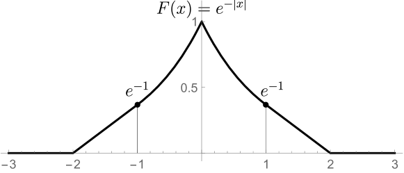
Figure 9: An example of a positive definite Pólya spline extension. (For visual effect we use different scales on the two coordinate axes.)

Theorem 12.22.

Let $G$ be a locally compact Abelian group. Let $\Omega\subset G$, $\Omega\neq\emptyset$, open and connected. Let $F:\Omega-\Omega\rightarrow\mathbb{C}$ be continuous, positive definite; and assume $Ext\left(F\right)\neq\emptyset$. Let $\mu\in Ext\left(F\right)$, and let $T_{\mu}\left(F_{\phi}\right):=\widehat{\varphi}$, defined initially only for $\varphi\in C_{c}\left(\Omega\right)$, be the isometry $T_{\mu}:\mathscr{H}_{F}\rightarrow L^{2}\left(\mu\right):=L^{2}(\widehat{G},\mu)$.

Then $Q_{\mu}:=T_{\mu}T_{\mu}^{*}$ is a projection in $L^{2}\left(\mu\right)$ onto $ran\left(T_{\mu}\right)$; and $ran\left(T_{\mu}\right)$ is the $L^{2}\left(\mu\right)$-closure of the span of the functions $\left\{e_{x}\>|\>x\in\overline{\Omega}\right\}$, where $e_{x}\left(\lambda\right):=\left\langle\lambda,x\right\rangle$, $\forall\lambda\in\widehat{G}$, and $\left\langle\lambda,x\right\rangle$ denotes the $\widehat{G}\leftrightarrow G$ duality.

Proof 12.23.

By Theorem 12.12, $T_{\mu}:\mathscr{H}_{F}\rightarrow L^{2}\left(\mu\right)$ is isometric, and so $Q_{\mu}:=T_{\mu}T_{\mu}^{*}$ is the projection in $L^{2}\left(\mu\right)$ onto $ran\left(T_{\mu}\right)$.

We shall need the following three facts:

1. $ran\left(T_{\mu}\right)=\left(null\left(T_{\mu}^{*}\right)\right)^{\perp}$, where “$\perp$” refers to the standard inner product in $L^{2}\left(\mu\right)$.

2. $\left(T_{\mu}^{*}f\right)\left(x\right)=\chi_{\overline{\Omega}}\left(x\right)\left(fd\mu\right)^{\vee}\left(x\right)$, $x\in G$.

3. Setting $e_{x}\left(\lambda\right)=\lambda\left(x\right)=\left\langle\lambda,x\right\rangle$, $x\in\overline{\Omega}$, $\forall\lambda\in\widehat{G}$, and

   $$E_{\mu}\left(\overline{\Omega}\right)=\overline{span}^{L^{2}\left(\mu\right)\mbox{-closure}}\left\{e_{x}\left(\cdot\right)\>|\>x\in\overline{\Omega}\right\},$$

   we note that $e_{x}\in ran\left(T_{\mu}\right)$, for all $x\in\overline{\Omega}$.

Comments. (1) is general for isometries in Hilbert space. (2) is from Corollary 12.15. Finally, (3) follows from Corollary 7.10.

Now, let $f\in L^{2}\left(\mu\right)$; we then have the following double-implications:

$$f \in \left(ran\left(T_{\mu}\right)\right)^{\perp}$$

$$\Updownarrow \left(\ref{enu:io1}\right)$$ by

$$\left(fd\mu\right)^{\vee}\left(x\right) = 0,\;\forall x\in\overline{\Omega}$$

$$\Updownarrow \left(\ref{enu:io2}\right)$$ by

$$\int_{\widehat{G}}\overline{\left\langle\lambda,x\right\rangle}f\left(\lambda\right)d\mu\left(\lambda\right) = 0,\;\forall x\in\overline{\Omega}$$

$$\Updownarrow$$

$$\left\langle e_{x},f\right\rangle_{L^{2}\left(\mu\right)} = 0,\;\forall x\in\overline{\Omega}.$$

Now applying “$\perp$” one more time, we get that

$$ran\left(T_{\mu}\right)=\left\{e_{x}\>|\>x\in\overline{\Omega}\right\}^{\perp\perp}=E_{\mu}\left(\overline{\Omega}\right),$$

which is the desired conclusion.     ∎

13 Lie Groups

In this section, we consider the extension problem for continuous positive definite functions in Lie groups.

A key ingredient in our approach to extensions of locally defined positive definite functions, in the context of Lie groups, is the use of a correspondence between the following two aspects of representation theory:

1. Unitary representations $U$ of a particular Lie group $G$, with $U$ acting in some Hilbert space $\mathscr{H}$; and

2. a derived representations $dU$ of the associated Lie algebra $La(G)$.

This viewpoint originate with two landmark papers by Nelson Nel (59), and Nelson-Stinespring NS (59).

The following observations about (ii) will be used without further mention in our discussion below, and elsewhere: First, given $U$, the derived representation $dU$ of $La(G)$ is a representation by unbounded skew-Hermitian operators $dU(X)$, for $X\in La\left(G\right)$, with common dense domain in the Hilbert space $\mathscr{H}$.

To say that $dU$ is a representation refers to the Lie bracket in $La(G)$ on one side, and the commutator bracket for operators on the other. Further, $dU$, as a representation of $La(G)$, automatically induces a representation of the corresponding associative enveloping algebra to $La(G)$; this is the one referenced in Nelson-Stinespring NS (59). But the most important point is that the correspondence from (i) to (ii) is automatic, while the reverse from (ii) to (i) is not. For example, the Lie algebra can only account for the subgroup of $G$ which is the connected component of the unit element in $G$. And, similarly, loops in $G$ cannot be accounted for by the Lie algebra. So, at best, a given representation $\rho$ of the Lie algebra will give information only about possible associated unitary representations of the universal covering group to $G$; the two have the same Lie algebra. But even then, there may not be a unitary representation of this group coming as an integral of a Lie algebra representation $\rho$: This is where the Laplace operator $\Delta$ of $G$ comes in. Nelson’s theorem states that a given Lie algebra representation $\rho$ is integrable (to a unitary representation) if and only if $\rho\left(\Delta\right)$ is essentially selfadjoint.

For a systematic account of the theory of integration of representations of Lie algebras in infinite dimensional Hilbert space, and their applications to physics, see JM (84).

Definition 13.1.

Let $G$ be a Lie group. Assume $\Omega\subset G$ is a non-empty, connected and open subset. A continuous

$$F:\Omega^{-1}\Omega\rightarrow\mathbb{C}$$ (137)

is said to be positive definite, iff (Def)

$$\sum\nolimits_{i}\sum\nolimits_{i}\overline{c_{i}}c_{j}F\left(x_{i}^{-1}x_{j}\right)\geq 0,$$ (138)

for all finite systems $\left\{c_{i}\right\}\subset\mathbb{C}$, and points $\left\{x_{i}\right\}\subset\Omega$. Equivalent,

$$\int_{\Omega}\overline{\varphi\left(x\right)}\varphi\left(y\right)F\left(x^{-1}y\right)dxdy\geq 0,$$ (139)

for all $\varphi\in C_{c}\left(\Omega\right)$; where $dx$ denotes a choice of left-invariant Haar measure on $G$.

Lemma 13.2.

1. Let $F$ be as in (137)-(138). For all $X\in La$$\left(G\right)=$ the Lie algebra of $G$, set

   $$(\widetilde{X}\varphi)\left(g\right)=\frac{d}{dt}\Big{|}_{t=0}\varphi\left(\exp_{G}\left(-tX\right)g\right),\quad\varphi\in C_{c}^{\infty}\left(\Omega\right).$$ (140)

   Let

   $$F_{\varphi}\left(x\right)=\int_{\Omega}\varphi\left(y\right)F\left(x^{-1}y\right)dy\,;$$ (141)

   then

   $$S_{X}^{\left(F\right)}:F_{\varphi}\longmapsto F_{\widetilde{X}\varphi},\quad\varphi\in C_{c}^{\infty}\left(\Omega\right)$$ (142)

   defines a representation of the Lie algebra $La\left(G\right)$ by skew-Hermitian operators in the RKHS $\mathscr{H}_{F}$, with the operator in (142) defined on the common dense domain $\left\{F_{\varphi}\>\big{|}\>\varphi\in C_{c}^{\infty}\left(\Omega\right)\right\}\subset\mathscr{H}_{F}$.

2. Let $F$ be as in part (1) above, and define $F_{\varphi}$ for $\varphi\in C_{c}^{\infty}\left(\Omega\right)$ as in (141), then $F_{\varphi}\in C^{\infty}\left(\Omega\right)$, and

   $$\widetilde{X}(F_{\varphi})=F_{\widetilde{X}\varphi}$$ (143)

   holds on $\Omega$, where $\widetilde{X}$ for $X\in La\left(G\right)$ is the vector field defined in (140).

Proof 13.3.

Part (1). The arguments here follow those of the proof of Lemma 8.3 mutatis mutandis.

Part (2). Let $F,\Omega,\varphi$, and $X$ be as in the statement of the theorem, and let $g\in\Omega$ be fixed. Then the r.h.s. in (143) exists as a pointwise limit as follows:

Let $t\in\mathbb{R}\backslash\left\{0\right\}$ be sufficiently small, i.e., $\left|t\right|<a$; then

$$\frac{1}{t}\left(F_{\varphi}\left(\exp_{G}\left(-tX\right)g\right)-F_{\varphi}\left(g\right)\right)$$

$$\overset{\begin{pmatrix}\mbox{invariance of}\\ \mbox{Haar measure}\end{pmatrix}}{=} \int_{\Omega}\frac{1}{t}\left(\varphi\left(\exp_{G}\left(-tX\right)y\right)-\varphi\left(y\right)\right)F\left(g^{-1}y\right)dy$$

$$\xrightarrow{\quad t\rightarrow 0\quad} \int_{\Omega}(\widetilde{X}\varphi)\left(y\right)F\left(g^{-1}y\right)dy=F_{\widetilde{X}\varphi}\left(g\right),$$

and the desired conclusion (143) follows, i.e., the function $F_{\varphi}$ is differentiable on the open set $\Omega$, with derivative as specified w.r.t. the vector field $\widetilde{X}$.

Note that $X\in La\left(G\right)$ is arbitrary. Since $\widetilde{X}\varphi\in C_{c}^{\infty}\left(\Omega\right)$, the argument may be iterated; so we get $F_{\varphi}\in C^{\infty}\left(\Omega\right)$ as desired.     ∎

Definition 13.4.

Let $\Omega\subset G$, non-empty, open and connected.

1. A continuous p.d. function $F:\Omega^{-1}\Omega\rightarrow\mathbb{C}$ is said to be extendable, if there is a continuous p.d. function $F_{ex}:G\rightarrow G$ such that

   $$F_{ex}\big{|}{}_{\Omega^{-1}\Omega}=F.$$ (144)

2. Let $U\in Rep\left(G,\mathscr{K}\right)$ be a strongly continuous unitary representation of $G$ acting in some Hilbert space $\mathscr{K}$. We say that $U\in Ext\left(F\right)$ (Section 10), if there is an isometry $J:\mathscr{H}_{F}\hookrightarrow\mathscr{K}$ such that the function

   $$G\ni g\longmapsto\left\langle JF_{e},U\left(g\right)JF_{e}\right\rangle_{\mathscr{K}}$$ (145)

   satisfies the condition (144)

Theorem 13.5.

Every extension of some continuous p.d. function $F$ on $\Omega^{-1}\Omega$ as in (1) arises from a unitary representation of $G$ as specified in (2).

Proof 13.6.

First assume some unitary representation $U$ of $G$ satisfies (2), then (145) is an extension of $F$. This follows from the argument in our proof of Theorem 9.1; also see Lemma 8.3 and 8.5.

For the converse; assume some continuous p.d. function $F_{ex}$ on $G$ satisfies (144). Now apply the GNS (Theorem 13.13) to $F_{ex}$; and, as a result, we get a cyclic representation $\left(U,\mathscr{K},v_{0}\right)$ where

• $\mathscr{K}$ is a Hilbert space;

• $U$ is a strongly continuous unitary representation of $G$ acting on $\mathscr{K}$; and

• $v_{0}\in\mathscr{K}$ is a cyclic vector, $\left\|v_{0}\right\|=1$; and

  $$F_{ex}\left(g\right)=\left\langle v_{0},U\left(g\right)v_{0}\right\rangle,\quad g\in G.$$ (146)

Defining $J:\mathscr{H}_{F}\rightarrow\mathscr{K}$ by

$$J\left(F\left(\cdot g\right)\right):=U\bigl{(}g^{-1}\bigr{)}v_{0},\quad\forall g\in\Omega;$$

and extend by limit. We check that $J$ is isometric and satisfies the condition from (2) in Definition 13.4. We omit details as they parallel the arguments already contained in Sections 7-10.

∎

Theorem 13.7.

Let $\Omega$, $G$, $La\left(G\right)$, and $F:\Omega^{-1}\Omega\rightarrow\mathbb{C}$ be as above. Let $\widetilde{G}$ be the simply connected universal covering group for $G$. Then $F$ has an extension to a p.d. continuous function on $\widetilde{G}$ iff there is a unitary representation $U$ of $\widetilde{G}$, and an isometry $\mathscr{H}_{F}\overset{J}{\longrightarrow}\mathscr{K}$, such that

$$JS_{X}^{\left(F\right)}=dU\left(X\right)J$$ (147)

holds on $\left\{F_{\varphi}\>\big{|}\>\varphi\in C_{c}^{\infty}\left(\Omega\right)\right\}$, for all $X\in La\left(G\right)$; where

$$dU\left(X\right)U\left(\varphi\right)v_{0}=U\bigl{(}\widetilde{X}\varphi\bigr{)}v_{0}.$$

Proof 13.8.

Details are contained in Sections 9, 15, and Chapter 5.     ∎

Assume $G$ is connected. On $C_{c}^{\infty}\left(\Omega\right)$, the Lie group $G$ acts locally by $\varphi\mapsto\varphi_{g}$, where $\varphi_{g}:=\varphi\left(g^{-1}\cdot\right)$ denotes translation of $\varphi$ by $g\in G$, such that $\varphi_{g}$ is also supported in $\Omega$. Note that

$$\left\|F_{\varphi}\right\|_{\mathscr{H}_{F}}=\left\|F_{\varphi_{g}}\right\|_{\mathscr{H}_{F}};$$ (148)

but only for elements $g\in G$ in a neighborhood of $e\in G$ , and with the neighborhood depending on $\varphi$.

Corollary 13.9.

Given

$$F:\Omega^{-1}\cdot\Omega\rightarrow\mathbb{C}$$ (149)

continuous and positive definite, then set

$$L_{g}\left(F_{\varphi}\right):=F_{\varphi_{g}},\quad\varphi\in C_{c}^{\infty}\left(\Omega\right),$$ (150)

defining a local representation of $G$ in $\mathscr{H}_{F}$.

Proof 13.10.

See Jor (87, 86); JT14a . Equivalently, introducing the Hilbert space $\mathfrak{M}_{2}\left(\Omega,F\right)$ from Corollary 7.10, i.e., all complex measures $\nu$ on $\Omega$ s.t.

$$\left\|\nu\right\|_{\mathfrak{M}_{2}\left(\Omega,F\right)}^{2}=\int_{\Omega}\int_{\Omega}F\left(x^{-1}y\right)\overline{d\nu\left(x\right)}d\nu\left(y\right)<\infty,$$

we get the following formula for the local representation $L$:

For elements $x,y\in\Omega$ s.t. $xy\in\Omega$, we have

$$L\left(x\right)\delta_{y}=\delta_{xy},\quad\mbox{and}\quad\left\langle\delta_{e},L\left(x\right)\delta_{e}\right\rangle_{\mathfrak{M}_{2}\left(\Omega,F\right)}=F\left(x\right)$$

holds.     ∎

Corollary 13.11.

Given $F$, positive definite and continuous, as in (149), and let $L$ be the corresponding local representation of $G$ acting on $\mathscr{H}_{F}$. Then $Ext\left(F\right)\neq\emptyset$ if and only if the local representation (150) extends to a global unitary representation acting in some Hilbert space $\mathscr{K}$, containing $\mathscr{H}_{F}$ isometrically.

Proof 13.12.

We refer to Jor (87, 86) for details, as well as Chapter 6.     ∎

13.1 The GNS Construction

Given a group $G$, or $C^{*}$-algebra $\mathfrak{A}$, the Gelfand–Naimark–Segal (GNS for short) construction establishes an explicit correspondence between representations on the one side and positive definite functionals (states) in the case of $C^{*}$-algebras, and positive definite functions in the case of groups. The non-trivial part is the construction of the representation from the given positive definite object. In the case of $C^{*}$-algebras the correspondence is between cyclic $*$-representations of $\mathfrak{A}$ and certain linear functionals on $\mathfrak{A}$ (called states). The correspondence is shown by an explicit construction of the $*$-representation from the state. In the case of groups $G$, the correspondence is between unitary representations of $G$, with cyclic vectors, on the one side, and positive definite functions $F$ on $G$ on the other. One further shows that the given p.d. function $F$ on $G$ is continuous iff the corresponding unitary representation is strongly continuous.

The following is the version of the GNS construction most relevant for our preset purpose. The construction is named after Israel Gelfand, Mark Naimark, and Irving Segal; and it is abbreviated the GNS construction Dix (96).

Theorem 13.13.

Let $G$ be a group, and let $F$ be a positive definite (p.d.) function on $G$, i.e., for all $\left\{x_{i}\right\}_{i=1}^{n}\subset G$, the $n\times n$ matrix $\left[F\left(x_{i}^{-1}x_{j}\right)\right]_{i,j=1}^{n}$ is assumed positive semidefinite. Assume $F\left(e\right)=1$.

1. Then there is a Hilbert space $\mathscr{H}$, a vector $v_{0}\in\mathscr{H}$, $\left\|v_{0}\right\|=1$, and a unitary representation $U$,

   $$U:G\rightarrow\left(\mbox{unitary operators on }\mathscr{H}\right),\;\mbox{s.t.}$$ (151)

   $$F\left(x\right)=\left\langle v_{0},U\left(x\right)v_{0}\right\rangle_{\mathscr{H}},\quad\forall x\in G.$$ (152)

2. The triple $\left(\mathscr{H},v_{0},U\right)$ may be chosen such that $v_{0}$ is a cyclic vector for the unitary representation in (151). (We shall do this.)

3. If $(\mathscr{H}_{i},v_{0}^{\left(i\right)},U_{i})$, $i=1,2$, are two solutions to the problem in (1)-(2), i.e.,

   $$F\left(x\right)=\left\langle v_{0}^{\left(i\right)},U_{i}\left(x\right)v_{0}^{\left(i\right)}\right\rangle_{\mathscr{H}_{i}},\;i=1,2$$ (153)

   holds for all $x\in G$; then there is an isometric intertwining isomorphism
   $W:\mathscr{H}_{1}\rightarrow\mathscr{H}_{2}$ (onto $\mathscr{H}_{2}$) such that

   $$WU_{1}\left(x\right)=U_{2}\left(x\right)W$$ (154)

   holds on $\mathscr{H}_{1}$, for all $x\in G$, the intertwining property.

Proof 13.14.

We shall refer to Dix (96) for details. The main ideas are sketched below:

Starting with a given $F:G\rightarrow\mathbb{C}$, p.d., as in the statement of the theorem, we build the Hilbert space (from part (1)) as follows:

Begin with the space of all finitely supported functions $\psi:G\rightarrow\mathbb{C}$, denoted by $Fun_{fin}\left(G\right)$. For $\varphi,\psi\in Fun_{fin}\left(G\right)$, set

$$\left\langle\varphi,\psi\right\rangle_{\mathscr{H}}:=\sum_{x}\sum_{y}\overline{\varphi\left(x\right)}\psi\left(y\right)F\left(x^{-1}y\right).$$ (155)

From the definition, it follows that

$$\left\langle\psi,\psi\right\rangle_{\mathscr{H}}\geq 0,\quad\forall\psi\in Fun_{fin}\left(G\right);$$

and moreover, that

$$N_{F}=\left\{\psi\>|\>\left\langle\psi,\psi\right\rangle_{\mathscr{H}}=0\right\}$$

is a subspace of $Fun_{fin}\left(G\right)$. To get $\mathscr{H}\left(=\mathscr{H}_{F}\right)$ as a Hilbert space, we do the following two steps:

$$Fun_{fin}\left(G\right)\xrightarrow[\left(\text{quotient}\right)]{}Fun_{fin}\left(G\right)/N_{F}\xrightarrow[\left(\text{Hilbert completion}\right)]{}\mathscr{H}.$$ (156)

For $v_{0}\in\mathscr{H}$, we choose

$$v_{0}=\mbox{class}\left(\delta_{e}\right)=\left(\delta_{e}+N_{F}\right)\in\mathscr{H},\;\mbox{see}\;\left(\ref{eq:gns6}\right).$$ (157)

In particular, for all $\varphi,\psi\in Fun_{fin}\left(G\right)$ and $g\in G$, we have

$$\left\langle\varphi\left(g^{-1}\cdot\right),\psi\left(g^{-1}\cdot\right)\right\rangle_{\mathscr{H}} = \sum_{x}\sum_{y}\overline{\varphi\left(x\right)}\psi\left(y\right)F\left(x^{-1}y\right)$$

$$= \left\langle\varphi,\psi\right\rangle_{\mathscr{H}},\;\mbox{see}\;\left(\ref{eq:gns5}\right).$$

Set $U\left(g\right)\psi=\psi\left(g^{-1}\cdot\right)$, i.e.,

$$\left(U\left(g\right)\psi\right)\left(x\right)=\psi\left(g^{-1}x\right),\quad x\in G.$$ (158)

Using (155)-(157), it is clear that $U$ as defined in (158) passes to the quotient and the Hilbert completion from (156), and that it will be the solution to our problem.

Finally, the uniqueness part of the theorem is left for the reader. See, e.g., Dix (96).     ∎

Corollary 13.15.

Assume that the group $G$ is a topological group. Let $F$ be a p.d. function specified as in Theorem 13.13 (1), and let $\left(\mathscr{H}_{F},v_{0},U\right)$ be the representation triple (cyclic, see part (2) of the theorem), solving the GNS problem. Then $F$ is continuous if and only if the representation $U$ is strongly continuous, i.e., if, for all $\psi\in\mathscr{H}_{F}$, the function

$$G\ni x\longmapsto U\left(x\right)\psi\in\mathscr{H}_{F}$$

is continuous in the norm of $\mathscr{H}_{F}$; iff for all $\varphi,\psi\in\mathscr{H}_{F}$, the function

$$F_{\varphi,\psi}\left(x\right)=\left\langle\varphi,U\left(x\right)\psi\right\rangle_{\mathscr{H}_{F}}$$

is continuous on $G$.

13.2 Local Representations

Definition 13.16.

Let $G$ be a Lie group and let $\mathscr{O}$ be an open connected neighborhood of $e\in G$. A local representation (defined on $\mathscr{O}$) is a function:

$$L:\mathscr{O}\longrightarrow\left(\mbox{isometric operators in some Hilbert space $\mathscr{H}$}\right)$$

such that

$$L\left(e\right)=I_{\mathscr{H}}\left(=\mbox{the identity operator in $\mathscr{H}$}\right);$$ (159)

and if $x,y\in\mathscr{O}$, and $xy\in\mathscr{O}$ as well, then

$$L\left(xy\right)=L\left(x\right)L\left(y\right),$$ (160)

where $xy$ denotes the group operation from $G$.

Theorem 13.17 (GNS for local representations).

Let $G$ be as above, and let $\Omega\subset G$ be an open connected subset. Set

$$\mathscr{O}=\Omega^{-1}\Omega=\left\{x^{-1}y\>|\>x,y\in\Omega\right\}.$$ (161)

Let $F$ be a continuous (locally defined) p.d. function on $\mathscr{O}=\Omega^{-1}\Omega$; and assume $F\left(e\right)=1$.

1. Then there is a triple $\left(\mathscr{H},v_{0},L\right)$, where $\mathscr{H}$ is a Hilbert space, $v_{0}\in\mathscr{H}$, $\left\|v_{0}\right\|=1$, and $L$ is an $\mathscr{O}$-local representation, strongly continuous, such that

   $$F\left(x\right)=\left\langle v_{0},L\left(x\right)v_{0}\right\rangle_{\mathscr{H}},\quad\forall x\in\mathscr{O}.$$ (162)

2. If $L$ is cyclic w.r.t. $v_{0}$, then the solution $\left(\mathscr{H},v_{0},L\right)$ is unique up to unitary equivalence.

3. Assume $L$ is cyclic; then on the dense subspace $\mathscr{D}_{L}$ of vectors spanned by

   $$L_{\varphi}v_{0}=\int_{\mathscr{O}}\varphi\left(x\right)L\left(x\right)v_{0}dx,\quad\varphi\in C_{c}^{\infty}\left(\mathscr{O}\right)$$ (163)

   (integration w.r.t. a choice of a left-Haar measure on $G$), we get a representation of the Lie algebra, $La\left(G\right)$ of $G$, acting as follows:
   Set $\lambda:=dL$, and

   $$\lambda\left(X\right)L_{\varphi}:=L_{\widetilde{X}\varphi}$$ (164)

   where $\widetilde{X}=$ the vector field (140). Specifically, on $\mathscr{D}_{L}$, we have,

   $$\lambda\left(\left[X,Y\right]\right) = \left[\lambda\left(X\right),\lambda\left(X\right)\right]$$

   $$= \lambda\left(X\right)\lambda\left(Y\right)-\lambda\left(Y\right)\lambda\left(X\right)$$

   (commutator), for all $X,Y\in La\left(G\right)$, where $\left[X,Y\right]$ on the l.h.s. in (3) denotes the Lie bracket from $La\left(G\right)$.

Proof 13.18.

The reader will notice that the proof of these assertions follows closely those details outlined in the proofs of the results from Sections 8.1, 13 and 13.1, especially Theorem 13.13 and Corollary 13.15. The reader will easily be able to fill in details; but see also JT14a .     ∎

Corollary 13.19.

Let $G$ be a connected locally compact group, and let $\mathscr{O}$ be an open neighborhood of $e$ in $G$. Let $F$ be a continuous positive definite function, defined on $\mathscr{O}$, and let $\widetilde{F}$ be a positive definite extension of $F$ to $G$; then $\widetilde{F}$ is continuous on $G$.

Proof 13.20.

Using Theorems 13.13 and 13.17, we may realize both $F$ and $\widetilde{F}$ in GNS-representations, yielding a local representation $L$ for $F$, and a unitary representation $U$ for the p.d. extension $\widetilde{F}$. This can be done in such a way that $U$ is an extension of $L$, i.e., extending from $\mathscr{O}$ to $G$. Since $F$ is continuous, it follows that $L$ is strongly continuous. But it is known that a unitary representation (of a connected $G$) is strongly continuous iff it is strongly continuous in a neighborhood of $e$. The result now follows from Corollary 13.15.     ∎

Remark 13.21.

It is not always possible to extend continuous p.d. functions $F$ defined on open subsets $\mathscr{O}$ in Lie groups. In Section 19 we give examples of locally defined p.d. functions $F$ on $G=\mathbb{R}^{2}$, i.e., $F$ defined on some open subset $\mathscr{O}\subset\mathbb{R}^{2}$ for which $Ext\left(F\right)=\emptyset$. But when extension is possible, the following algorithm applies, see Figure 10; also compare with Figure 7 in the case of $G=\mathbb{R}$.

Figure 10: Extension correspondence. From locally defined p.d. function $F$ to local representation $L$, to representation of the Lie algebra, to a unitary representation $U$ of $G$, and finally to an element in $Ext(F)$.

13.3 The Convex Operation in $Ext\left(F\right)$

Definition 13.22.

Let $G$, $\Omega$, $\mathscr{O}=\Omega^{-1}\Omega$, and $F$ be as in the statement of Theorem 13.17; i.e., $F$ is a given continuous p.d. function, locally defined in $G$. Assume $F\left(e\right)=1$.

Using Theorem 13.13, we consider “points” in $Ext\left(F\right)$ to be triples $\pi:=(\mathscr{H},U,v^{\left(0\right)})$ specified as in (1)-(2) of the theorem; i.e.,

• Hilbert space

• strongly continuous unitary representation of $G$

• vector in $\mathscr{H}$ s.t. $\|v^{\left(0\right)}\|_{\mathscr{H}}=1$.

Moreover, the restriction property

$$F\left(x\right)=\left\langle v^{\left(0\right)},U\left(x\right)v^{\left(0\right)}\right\rangle_{\mathscr{H}},\quad x\in\mathscr{O},$$ (166)

holds. Denote the r.h.s. in (166), $\widetilde{F}_{\pi}$.

Now let $\alpha\in\mathbb{R}$ satisfying $0<\alpha<1$, and let $\pi_{i}=(\mathscr{H}_{i},U_{i},v_{i}^{\left(0\right)})$, $i=1,2$, be two “points” in $Ext\left(F\right)$; in particular, (166) holds for both $\pi_{1}$ and $\pi_{2}$. The convex combination is

$$\pi=\alpha\pi_{1}+\left(1-\alpha\right)\pi_{2}.$$ (167)

It is realized as follows:

Set $\mathscr{H}:=\mathscr{H}_{1}\oplus\mathscr{H}_{2}$, $U:=U_{1}\oplus U_{2}$, and

$$v^{\left(0\right)}=\sqrt{\alpha}v_{1}^{\left(0\right)}+\sqrt{1-\alpha}v_{2}^{\left(0\right)}\in\mathscr{H}=\mathscr{H}_{1}\oplus\mathscr{H}_{2};$$ (168)

those are the standard direct sum operations in Hilbert space.

Claim 2.

The function

$$\widetilde{F}\left(x\right)=\left\langle v^{\left(0\right)},U\left(x\right)v^{\left(0\right)}\right\rangle_{\mathscr{H}},\quad x\in G$$

satisfies (166), and so it is in $Ext\left(F\right)$.

Proof 13.23.

Setting

$$\widetilde{F}_{i}\left(x\right)=\left\langle v_{i}^{\left(0\right)},U_{i}\left(x\right)v_{i}^{\left(0\right)}\right\rangle_{\mathscr{H}_{i}},\;i=1,2,\;\mbox{and }x\in G.$$ (169)

Then, using (168), one easily verifies that

$$\widetilde{F}\left(x\right)=\alpha\widetilde{F}_{1}\left(x\right)+\left(1-\alpha\right)\widetilde{F}_{2}\left(x\right)$$ (170)

holds for all $x\in G$; and the desired conclusion follows.     ∎

Remark 13.24.

Using Definition 13.22, one now checks that, for Examples 1-5 in Table 1 below, we get that

$$Ext_{1}\left(F\right)\subseteq ext\left(Ext\left(F\right)\right)$$ (171)

where the “ext” on the r.h.s. in (171) denotes the set of extreme points in $Ext\left(F\right)$, in the sense of Krein-Milman Phe (66).

In general, (171) is a proper containment.

Example 13.25.

Below we illustrate (171) in Remark 13.24 with $F=F_{3}$ from Table 1, i.e., $F\left(t\right)=e^{-\left|t\right|}$ in $\left|t\right|<1$; $G=\mathbb{G}$, and $\Omega=\left(0,1\right)$. In this case, the skew-Hermitian operator $D^{\left(F\right)}$ from Section 8 has deficiency $\left(1,1\right)$. Using the discussion above, one sees that every “point” $\pi=(\mathscr{H}^{\left(\pi\right)},U^{\left(\pi\right)},v^{\left(\pi\right)})$ in the closed convex hull, $\overline{conv}Ext_{1}\left(F\right)$, of $Ext_{1}\left(F\right)$ has the following form. (See, e.g., Phe (66).)

Fix such a $\pi$. There is then a unique probability measure $\rho^{\pi}$ on $\mathbb{T}=\mathbb{R}/\mathbb{Z}$ such that, up to unitary equivalence, the three components of $\pi$ are as follows:

• $\mathscr{H}^{\left(\pi\right)}$: measurable functions $f$ on $\mathbb{R}\times\mathbb{T}$ such that

  $$\chi_{\left[0,1\right]}\left(\cdot\right)f\left(\cdot,\alpha\right)\in\mathscr{H}_{F},\quad\alpha\in\mathbb{T};$$ (172)

  $$\left(f+f^{\prime}\right)\left(x+n,\alpha\right)=\alpha^{n}\left(f-f^{\prime}\right)\left(x,\alpha\right),\quad\forall x\in\mathbb{R},\>n\in\mathbb{Z},\>\alpha\in\mathbb{T};$$ (173)

  where $f$ is $C^{1}$ in the $x$-variable (in $\mathbb{R}$), and measurable in $\alpha$ (in $\mathbb{T}$). And

  $$\left\|f\right\|_{\mathscr{H}^{\left(\pi\right)}}^{2}:=\int_{\mathbb{T}}\left\|\chi_{\left[0,1\right]}\left(\cdot\right)f\left(\cdot,\alpha\right)\right\|_{\mathscr{H}_{F}}^{2}d\alpha^{\left(Haar\right)}<\infty,$$ (174)

  where $d\alpha$ is the Haar measure on $\mathbb{T}$, i.e, $\alpha=e^{i2\pi\theta}$, $0\leq\theta\leq 1$, yields

  $$d\alpha^{\left(Haar\right)}=d\theta.$$

  Set

  $$\mathscr{H}^{\left(\pi\right)}=\int_{\mathbb{T}}^{\oplus}\mathscr{H}_{F}d\rho^{\left(\pi\right)},$$ (175)

  as a direct integral.

Remark 13.26.

Eq (173) above is a “boundary-condition.” In detail: For fixed $\alpha\in\mathbb{T}$, this condition comes from the von Neumann extension corresponding to the deficiency analysis of our skew-Hermitian operator $D^{\left(F\right)}$. More specifically, recall that, as an operator in $\mathscr{H}_{F}$ (with dense domain), $D^{\left(F\right)}$ has deficiency indices $\left(1,1\right)$ and so, by our analysis in Section 18, every $\alpha\in\mathbb{T}$ corresponds to a unique skew-adjoint extension $A^{\left(\alpha\right)}$ of $D^{\left(F\right)}$. The conditions in (173) simply allow us to realize the unitary one-parameter group $U\left(t\right)$ generated by $A^{\left(\alpha\right)}$, with $U\left(t\right)$ realized as per the specification in (178). For further details on boundary conditions in reproducing kernel Hilbert spaces of type $\mathscr{H}_{F}$, see JT14b .

• $U^{\left(\pi\right)}$: Up to unitary equivalence, we get

  $$U_{t}^{\left(\pi\right)}\left(f\left(\cdot,\alpha\right)\right)_{\alpha\in\mathbb{T}}\left(x\right):=\left(f\left(x+t,\alpha\right)\right)_{\alpha\in\mathbb{T}},\quad\forall t\in\mathbb{R};$$ (176)

  where we use the representation (175) above for $\mathscr{H}^{\left(\pi\right)}$.

• Finally, we have the following direct integral representation of the respective rank-one operators (using Dirac notation):

  $$\left|v^{\left(\pi\right)}\left\rangle\right\langle v^{\left(\pi\right)}\right|=\int_{\mathbb{T}}^{\oplus}d\rho^{\left(\pi\right)}\left(\alpha\right)\left|F_{0}\left\rangle\right\langle F_{0}\right|$$ (177)

  The ket-bra notation $\left|v\left\rangle\right\langle v\right|$ means rank-one operator.

For $\alpha\in\mathbb{T}$ fixed, we note that

$$\left(U_{t}^{\left(\alpha\right)}f\left(\cdot,\alpha\right)\right)\left(x\right)=f\left(x+t,\alpha\right),\quad t\in\mathbb{R},$$ (178)

represents a unique element in $Ext_{1}\left(F\right)$, and

$$U_{t}^{\left(\pi\right)}=\int_{\mathbb{T}}^{\oplus}U_{t}^{\left(\alpha\right)}d\rho^{\left(\pi\right)}\left(\alpha\right),\quad t\in\mathbb{\mathbb{R}}$$ (179)

is the unitary representation corresponding to $\pi$, i.e.,

$$\widetilde{F^{\left(\pi\right)}}\left(t\right)=\int_{\mathbb{T}}\widetilde{F^{\left(\alpha\right)}}\left(t\right)d\rho^{\left(\pi\right)}\left(\alpha\right),\quad t\in\mathbb{R};$$ (180)

and $\widetilde{F^{\left(\pi\right)}}\left(\cdot\right)$ is the continuous p.d. function on $\mathbb{R}$ which extends $F$ (on $\left(-1,1\right)$), and corresponding to the “point” $\pi\in\overline{conv}Ext_{1}\left(F\right)$ Phe (66).

The respective $\mathbb{R}$ p.d. functions in (180) are as follows:

$$\widetilde{F^{\left(\pi\right)}}\left(t\right)=\left\langle v^{\left(\pi\right)},U_{t}^{\left(\pi\right)}v^{\left(\pi\right)}\right\rangle_{\mathscr{H}^{\left(\pi\right)}},\quad t\in\mathbb{R},$$ (181)

and

$$\widetilde{F^{\left(\alpha\right)}}\left(t\right)=\left\langle F_{0},U_{t}^{\left(\alpha\right)}F_{0}\right\rangle_{\mathscr{H}_{F}},$$ (182)

defined for all $t\in\mathbb{R}$, and $\alpha\in\mathbb{T}$. For each $\alpha$ fixed, we have

$$U_{t}^{\left(\alpha\right)}=e^{tA^{\left(\alpha\right)}},\quad t\in\mathbb{R},$$ (183)

where $A^{\left(\alpha\right)}=-(A^{\left(\alpha\right)})^{*}$ is a skew-adjoint extension of $D^{\left(F\right)}$, acting in $\mathscr{H}_{F}$.

Remark 13.27.

In the direct-integral formulas (175) and (177), we stress that it is a direct integral of copies of the Hilbert space $\mathscr{H}_{F}$; more precisely, an isomorphic copy of $\mathscr{H}_{F}$ for every $\alpha\in\mathbb{T}$. For fixed $\alpha\in\mathbb{T}$, when we define our Hilbert space via eq (173), then we will automatically get the right boundary condition. They are built in. And on this Hilbert space, then the action of $U(t)$ will simplify; it will just be the translation formula (178). In fact, the construction is analogous to an induced representation Mac (88). We must also need to justify “up to unitary equivalence.” It is on account of Mackey’s imprimitivity theorem, see Ørs (79).

Our present direct integral representation should be compared with the Zak transform from signal processing Jan (03); ZM (95).

It was mathematics, the non-empirical science par excellence, wherein the mind appears to play only with itself, that turned out to be the science of sciences, delivering the key to those laws of nature and the universe that are concealed by appearances.
— Hannah Arendt, The Life of the Mind (1971), p.7.

Chapter 4 Examples

While the present chapter is made up of examples, we emphasis that the selection of examples is carefully chosen; – chosen and presented in such a way that the details involved, do in fact cover and illustrate general and important ideas, which in turn serve to bring out the structure of more general theorems (in the second half of our monograph.) Moreover, the connection from the examples to more general contexts will be mentioned inside the present chapter, on a case-by-case basis. We further emphasize that some of the examples have already been used to illustrate key ideas in Chapters 1 and 2 above. Below we flesh out the details. And our present examples will be used again in Chapters 6 through 11 below, dealing with theorems that apply to any number of a host of general settings.

14 The Case of $G=\mathbb{R}^{n}$

Of course, $G=\mathbb{R}^{n}$ is a special case of locally compact Abelian groups (Section 12), but the results available for $\mathbb{R}^{n}$ are more refined. We focus on this in the present section. This is also the setting of the more classical studies of the extension questions.

Let $\Omega\subset\mathbb{R}^{n}$ be a fixed open and connected subset; and let $F:\Omega-\Omega\rightarrow\mathbb{C}$ be a given continuous p.d. function, where

$$\Omega-\Omega:=\left\{x-y\in\mathbb{R}^{n}\>|\>x,y\in\Omega\right\}.$$ (184)

Let $\mathscr{H}_{F}$ be the corresponding reproducing kernel Hilbert space (RKHS).

We showed (Theorem 9.1) that $Ext\left(F\right)\not\neq\emptyset$ if and only if there is a strongly continuous unitary representation $\{U\left(t\right)\}_{t\in\mathbb{R}^{n}}$ acting on $\mathscr{H}_{F}$ such that

$$\mathbb{R}^{n}\ni t\longmapsto\left\langle F_{0},U\left(t\right)F_{0}\right\rangle_{\mathscr{H}_{F}}$$ (185)

is a p.d. extension of $F$, extending from (184) to $\mathbb{R}^{n}$.

Now if $U$ is a unitary representation of $G=\mathbb{R}^{n}$, we denote by $P_{U}\left(\cdot\right)$ the associated projection valued measure (PVM) on $\mathscr{B}\left(\mathbb{R}^{n}\right)$ (= the sigma–algebra of all Borel subsets in $\mathbb{R}^{n}$). We have

$$U\left(t\right)=\int_{\mathbb{R}^{n}}e^{it\cdot\lambda}P_{U}\left(d\lambda\right),\quad\forall t\in\mathbb{R}^{n};$$ (186)

where $t=\left(t_{1},\ldots,t_{n}\right)$, $\lambda=\left(\lambda_{1},\ldots,\lambda_{n}\right)$, and $t\cdot\lambda=\sum_{j=1}^{n}t_{j}\lambda_{j}$. Setting

$$d\mu\left(\cdot\right)=\left\|P_{U}\left(\cdot\right)F_{0}\right\|_{\mathscr{H}_{F}}^{2},$$ (187)

then the p.d. function on r.h.s. in (185) satisfies

$$r.h.s.\left(\ref{eq:rn2}\right)=\int_{\mathbb{R}^{n}}e^{it\cdot\lambda}d\mu\left(\lambda\right),\quad\forall t\in\mathbb{R}^{n}.$$ (188)

The purpose of the next theorem is to give an orthogonal splitting of the RKHS $\mathscr{H}_{F}$ associated to a fixed $\left(\Omega,F\right)$ when it is assumed that $Ext\left(F\right)$ is non-empty. This orthogonal splitting of $\mathscr{H}_{F}$ depends on a choice of $\mu\in Ext\left(F\right)$, and the splitting is into three orthogonal subspaces of $\mathscr{H}_{F}$, correspond a splitting of spectral types into atomic, absolutely continuous (with respect to Lebesgue measure), and singular.

Theorem 14.1.

Let $\Omega\subset\mathbb{R}^{n}$ be given, $\Omega\neq\emptyset$, open and connected. Suppose $F$ is given p.d. and continuous on $\Omega-\Omega$, and assume $Ext\left(F\right)\neq\emptyset$. Let $U$ be the corresponding unitary representations of $G=\mathbb{R}^{n}$, and let $P_{U}\left(\cdot\right)$ be its associated PVM acting on $\mathscr{H}_{F}$.

1. Then $\mathscr{H}_{F}$ splits up as an orthogonal sum of three closed and $U\left(\cdot\right)$-invariant subspaces

   $$\mathscr{H}_{F}=\mathscr{H}_{F}^{\left(atom\right)}\oplus\mathscr{H}_{F}^{\left(ac\right)}\oplus\mathscr{H}_{F}^{\left(sing\right)},$$ (189)

   characterized by the PVM $P_{U}$ as follows:

   1. $P_{U}$ restricted to $\mathscr{H}_{F}^{\left(atom\right)}$ is purely atomic;

   2. $P_{U}$ restricted to $\mathscr{H}_{F}^{\left(ac\right)}$ is absolutely continuous with respect to the Lebesgue measure on $\mathbb{R}^{n}$; and

   3. $P_{U}$ is continuous, purely singular, when restricted to $\mathscr{H}_{F}^{\left(sing\right)}$.

2. Case $\mathscr{H}_{F}^{\left(atom\right)}$. If $\lambda\in\mathbb{R}^{n}$ is an atom in $P_{U}$, i.e., $P_{U}\left(\left\{\lambda\right\}\right)\neq 0$, where $\left\{\lambda\right\}$ denotes the singleton with $\lambda$ fixed; then $P_{U}$$\left(\left\{\lambda\right\}\right)\mathscr{H}_{F}$ is one-dimensional. Moreover,

   $$P_{U}\left(\left\{\lambda\right\}\right)\mathscr{H}_{F}=\mathbb{C}e_{\lambda}\big{|}_{\Omega};$$ (190)

   where $e_{\lambda}\left(x\right):=e^{i\lambda\cdot x}$ is the complex exponential. In particular, $e_{\lambda}\big{|}_{\Omega}\in\mathscr{H}_{F}$.
   Case $\mathscr{H}_{F}^{\left(ac\right)}$. If $\xi\in\mathscr{H}_{F}^{\left(ac\right)}$, then it is represented as a continuous function on $\Omega$, and

   $$\left\langle\xi,F_{\varphi}\right\rangle_{\mathscr{H}_{F}}=\int_{\Omega}\overline{\xi\left(x\right)}\varphi\left(x\right)dx_{\text{(Lebesgue)}},\quad\forall\varphi\in C_{c}\left(\Omega\right).$$ (191)

   Further, there is a $f\in L^{2}\left(\mathbb{R}^{n},\mu\right)$ ($\mu$ as in (187)) such that, for all $\varphi\in C_{c}\left(\Omega\right)$,

   $$\int_{\Omega}\overline{\xi\left(x\right)}\varphi\left(x\right)dx=\int_{\mathbb{R}^{n}}\overline{f\left(\lambda\right)}\widehat{\varphi}\left(\lambda\right)d\mu\left(\lambda\right),\;\mbox{and}$$ (192)

   $$\xi=\left(fd\mu\right)^{\vee}\big{|}_{\Omega}.$$ (193)

   The r.h.s. of (193) is a $\mu$-extension of $\xi$. Consequently, every $\mu$-extension $\widetilde{\xi}$ of $\xi$ is continuos on $\mathbb{R}^{n}$, and $\lim_{\left|x\right|\rightarrow\infty}\widetilde{\xi}\left(x\right)=0$, i.e., $\widetilde{\xi}\in C_{0}\left(\mathbb{R}^{n}\right)$.
   
   Case $\mathscr{H}_{F}^{\left(sing\right)}$. Vectors $\xi\in\mathscr{H}_{F}^{\left(sing\right)}$ are characterized by the following property: The measure

   $$d\mu_{\xi}\left(\cdot\right):=\left\|P_{U}\left(\cdot\right)\xi\right\|_{\mathscr{H}_{F}}^{2}$$ (194)

   is continuous and purely singular.

Proof 14.2.

Most of the proof details are contained in the previous discussion. See Section 12, Theorem 12.12. For the second part of the theorem:

Case $\mathscr{H}_{F}^{\left(atom\right)}$. Suppose $\lambda\in(\mathbb{R}^{n})$ is an atom, and that $\xi\in\mathscr{H}_{F}\backslash\left\{0\right\}$ satisfies $P_{U}\left(\left\{\lambda\right\}\right)\xi=\xi$; then

$$U\left(t\right)\xi=e^{it\cdot\lambda}\xi,\quad\forall t\in\mathbb{R}^{n}.$$ (195)

By (185)-(186), we conclude that $\xi$ is a continuous, weak solution to the elliptic system

$$\frac{\partial}{\partial x_{j}}\xi=\sqrt{-1}\lambda_{j}\xi\>\left(\mbox{on }\Omega\right),\quad 1\leq j\leq n.$$ (196)

Hence $\xi=\mbox{const}\cdot e_{\lambda}|_{\Omega}$ as asserted in (190).

Case $\mathscr{H}_{F}^{\left(ac\right)}$; this follows from (193) and the Riemann-Lebesgue theorem applied to $\mathbb{R}^{n}$; and the case $\mathscr{H}_{F}^{\left(sing\right)}$ is immediate.     ∎

Example 14.3.

Consider the following continuous p.d. function $F$ on $\mathbb{R}$, or on some bounded interval $\left(-a,a\right)$, $a>0$.

$$F\left(x\right)=\frac{1}{3}\left(e^{-ix}+\prod_{n=1}^{\infty}\cos\left(\frac{2\pi x}{3^{n}}\right)+e^{i3x/2}\frac{\sin\left(x/2\right)}{\left(x/2\right)}\right).$$ (197)

The RKHS $\mathscr{H}_{F}$ has the decomposition (189), where all three subspaces $\mathscr{H}_{F}^{\left(atom\right)}$, $\mathscr{H}_{F}^{\left(ac\right)}$, and $\mathscr{H}_{F}^{\left(sing\right)}$ are non-zero; the first one is one-dimensional, and the other two are infinite-dimensional. Moreover, the operator

$$D^{\left(F\right)}\left(F_{\varphi}\right):=F_{\varphi^{\prime}}\mbox{ on}$$ (198)

$$dom\big{(}D^{\left(F\right)}\big{)}=\left\{F_{\varphi}\>\big{|}\>\varphi\in C_{c}^{\infty}\left(0,a\right)\right\}$$

is bounded, and so extends by closure to a skew-adjoint operator, satisfying

$$\overline{D^{\left(F\right)}}=-(D^{\left(F\right)})^{*}.$$

Proof 14.4.

Using infinite convolutions of operators (Chapter 9), and results from DJ (12), we conclude that $F$ defined in (197) is entire analytic, and $F=\widehat{d\mu}$ (Bochner-transform) where

$$d\mu\left(\lambda\right)=\frac{1}{3}\left(\delta_{-1}+\mu_{c}+\chi_{\left[1,2\right]}\left(\lambda\right)d\lambda\right).$$ (199)

The measures on the r.h.s. in (199) are as follows (Figure 11-12):

• $\delta_{-1}$ is the Dirac mass at $-1$, i.e., $\delta\left(\lambda+1\right)$.

• $\mu_{c}=$ the middle-third Cantor measure; determined as the unique solution in $\mathscr{M}_{+}^{prob}\left(\mathbb{R}\right)$ to

  $$\int f\left(\lambda\right)d\mu_{c}\left(\lambda\right)$$

  $$= \frac{1}{2}\left(\int f\left(\frac{\lambda+1}{3}\right)d\mu_{c}\left(\lambda\right)+\int f\left(\frac{\lambda-1}{3}\right)d\mu_{c}\left(\lambda\right)\right),\quad\forall f\in C_{c}\left(\mathbb{R}\right).$$

• $\chi_{\left[1,2\right]}\left(\lambda\right)d\lambda$ is restriction to the closed interval $\left[1,2\right]$ of Lebesgue measure.

It follows from the literature (e.g. DJ (12)) that $\mu_{c}$ is supported in $\left[-\frac{1}{2},\frac{1}{2}\right]$. Thus, the three measures on the r.h.s. in (199) have disjoint compact supports, with the three supports positively separately.

The conclusions asserted in Example 14.3 follow from this, in particular the properties for $D^{\left(F\right)}$. In fact,

$$\mbox{spectrum}(iD^{\left(F\right)})\subseteq\left\{-1\right\}\cup\left[-\tfrac{1}{2},\tfrac{1}{2}\right]\cup\left[1,2\right]\quad(i=\sqrt{-1})$$ (200)

∎

Figure 11: The measure $d\mu\left(\lambda\right)$ in Example 14.3.

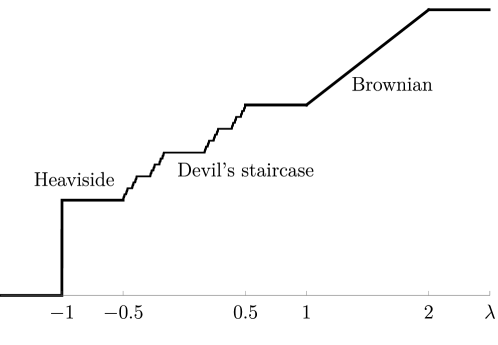
Figure 12: Cumulative distribution $=\int_{-\infty}^{\lambda}d\mu\left(\lambda\right)$, as in Example 14.3.

Corollary 14.5.

Let $\Omega\subset\mathbb{R}^{n}$ be non-empty, open and connected. Let $F:\Omega-\Omega\rightarrow\mathbb{C}$ be a fixed continuous and p.d. function; and let $\mathscr{H}_{F}$ be the corresponding RKHS (of functions on $\Omega$.)

1. If there is a compactly supported measure $\mu\in Ext\left(F\right)$, then every function $\xi$ on $\Omega$, which is in $\mathscr{H}_{F}$, has an entire analytic extension to $\mathbb{C}^{n}$, i.e., extension from $\Omega\subset\mathbb{R}^{n}$ to $\mathbb{C}^{n}$.

2. If, in addition, it is assumed that $\mu\ll d\lambda\left(=d\lambda_{1}\cdots d\lambda_{n}\right)=$ the Lebesgue measure on $\mathbb{R}^{n}$, where “$\ll$” means “absolutely continuous;” then the functions in $\mathscr{H}_{F}$ are restrictions to $\Omega$ of $C_{c}\left(\mathbb{R}^{n}\right)$-functions.

Proof 14.6.

Part (1). Let $\Omega$, $F$, $\mathscr{H}_{F}$ and $\mu$ be as stated. Let $\mathscr{H}_{F}\overset{T}{\longrightarrow}L^{2}\left(\mathbb{R}^{n},\mu\right)$ be the isometry from Corollary 12.15, where

$$T\left(F_{\varphi}\right):=\widehat{\varphi},\quad\varphi\in C_{c}\left(\Omega\right).$$ (201)

By (128), for all $f\in L^{2}\left(\mathbb{R}^{n},\mu\right)$, we have

$$\left(T^{*}f\right)\left(x\right)=\int_{\mathbb{R}^{n}}e^{ix\cdot\lambda}f\left(\lambda\right)d\mu\left(\lambda\right),\quad x\in\Omega;$$ (202)

Equivalently,

$$T^{*}f=\chi_{\overline{\Omega}}\left(fd\mu\right)^{\vee},\quad\forall f\in L^{2}\left(\mu\right).$$ (203)

And further that

$$T^{*}\left(L^{2}\left(\mathbb{R}^{n},\mu\right)\right)=\mathscr{H}_{F}.$$ (204)

Now, if $\mu$ is of compact support, then so is the complex measure $fd\mu$. This measure is finite since $L^{2}\left(\mu\right)\subset L^{1}\left(\mu\right)$. Hence the desired conclusion follows from (202), (204), and the Paley-Wiener theorem; see e.g., Rud (73).

Part (2) of the corollary follows from Theorem 14.1, case $\mathscr{H}_{F}^{\left(ac\right)}$. See also Proposition 18.14.

Details about (203): For all $f\in L^{2}\left(\mu\right)$, and all $\varphi\in C_{c}\left(\Omega\right)$, we have

$$\left\langle T(F_{\varphi}),f\right\rangle_{L^{2}\left(\mu\right)} = \int_{\mathbb{R}}\overline{\widehat{\varphi}\left(\lambda\right)}f\left(\lambda\right)d\mu\left(\lambda\right)$$

$$= \int_{\mathbb{R}}\left(\overline{\int_{\Omega}\varphi\left(x\right)e^{-i\lambda\cdot x}dx}\right)f\left(\lambda\right)d\mu\left(\lambda\right)$$

$$= \int_{\mathbb{R}}\left(\overline{\int_{\mathbb{R}}\chi_{\overline{\Omega}}\left(x\right)\varphi\left(x\right)e^{-i\lambda\cdot x}dx}\right)f\left(\lambda\right)d\mu\left(\lambda\right)$$

$$\underset{\left(\text{Fubini}\right)}{=} \int_{\mathbb{R}}\chi_{\overline{\Omega}}\left(x\right)\overline{\varphi\left(x\right)}\left(\int_{\mathbb{R}}e^{i\lambda\cdot x}f\left(\lambda\right)d\mu\left(\lambda\right)\right)dx$$

$$= \int_{\mathbb{R}}\overline{\varphi\left(x\right)}\left(\chi_{\overline{\Omega}}\left(fd\mu\right)^{\vee}\right)\left(x\right)dx$$

$$= \left\langle F_{\varphi},\chi_{\overline{\Omega}}\left(fd\mu\right)^{\vee}\right\rangle_{\mathscr{H}_{F}},$$

which is the desired conclusion.     ∎

15 The Case of $G=\mathbb{R}/\mathbb{Z}$

While we consider extensions of locally defined continuous and positive definite (p.d.) functions $F$ on groups, say $G$, the question of whether $G$ is simply connected or not plays an essential role in the analysis, and in the possible extensions.

It turns out that the geometric issues arising for general Lie groups can be illustrated well in a simple case. To illustrate this point, we isolate below the two groups, the circle group, and its universal cover, the real line. We study extensions defined on a small arc in the circle group $G=\mathbb{T}=\mathbb{R}/\mathbb{Z}$, versus extensions to the universal covering group $\mathbb{R}$.

Let $G=\mathbb{T}$ represented as $\left(-\tfrac{1}{2},\tfrac{1}{2}\right]$. Pick $0<\varepsilon<\tfrac{1}{2}$, and let $\Omega=\left(0,\varepsilon\right)$, so that $\Omega-\Omega=(-\varepsilon,\varepsilon)$ mod $\mathbb{Z}$.

Let $F:\Omega-\Omega\rightarrow\mathbb{C}$ be a continuous p.d. function; $D^{\left(F\right)}$ is the canonical skew-Hermitian operator, s.t. $dom(D^{\left(F\right)})=\{F_{\varphi}\>|\>\varphi\in C_{c}^{\infty}\left(\Omega\right)\}$, $D^{\left(F\right)}(F_{\varphi})=F_{\varphi^{\prime}}$, acting in the RKHS $\mathscr{H}_{F}$. As shown in Section 7, $D^{\left(F\right)}$ has deficiency indices $\left(0,0\right)$ or $\left(1,1\right)$.

Lemma 15.1.

If $D^{\left(F\right)}$ has deficiency indices $(1,1)$, there is a skew-adjoint extension of $D^{\left(F\right)}$ acting in $\mathscr{H}_{F}$, such that the corresponding p.d. extension $\widetilde{F}$ of $F$ has period one; then $\varepsilon$ is rational.

Proof 15.2.

In view of Section 10 (also see Theorem 9.1), our assumptions imply that that the dilation Hilbert space is identical to $\mathscr{H}_{F}$, thus an “internal” extension.

Since the deficiency indices of $D^{\left(F\right)}$ are $(1,1)$, the skew-adjoint extensions of $D^{(F)}$ are determined by boundary conditions of the form

$$\xi(\varepsilon)=e^{i\theta}\xi(0),$$ (205)

where $0\leq\theta<1$ is fixed.

Let $A_{\theta}$ be the extension corresponding to $\theta$, and

$$U_{A_{\theta}}\left(t\right)=e^{tA_{\theta}}=\int_{\mathbb{R}}e^{it\lambda}P_{A_{\theta}}(d\lambda),\quad t\in\mathbb{R}$$

be the corresponding unitary group, where $P_{A}\left(\cdot\right)$ is the projection-valued measure of $A_{\theta}$. Set

$$F_{A_{\theta}}(t)=\left\langle F_{0},U_{A_{\theta}}\left(t\right)F_{0}\right\rangle_{\mathscr{H}_{F}}=\int_{\mathbb{R}}e^{it\lambda}d\mu_{A_{\theta}}(\lambda)$$

where

$$d\mu_{A_{\theta}}(\lambda)=\left\|P_{A_{\theta}}(d\lambda)F_{0}\right\|_{\mathscr{H}_{F}}^{2}.$$

Repeating the calculation of the defect vectors and using that eigenfunctions of $A_{\theta}$ must satisfy the boundary condition (205), it follows that the spectrum of $A_{\theta}$ is given by

$$\sigma\left(iA_{\theta}\right)=\left\{\tfrac{\theta+n}{\varepsilon}\>|\>n\in\mathbb{Z}\right\}.$$

Note that $supp(\mu_{A_{\theta}})\subset\sigma\left(iA_{\theta}\right)$, and the containment becomes equal if $F_{0}$ is a cyclic vector for $U_{A_{\theta}}\left(t\right)$. Since $F_{A}$ is assumed to have period one, $supp(\mu_{A_{\theta}})$ consists of integers. Now if $\lambda_{n},\lambda_{m}\in supp(\mu_{A_{\theta}})$, then

$$\varepsilon=\frac{n-m}{\lambda_{n}-\lambda_{m}}$$

which is rational.     ∎

Remark 15.3.

If

$$F\left(x\right)=e^{-\left|x\right|},\quad-\pi<x\leq\pi$$ (206)

is considered a function on $\mathbb{T}$ via $\mathbb{T}=\mathbb{R}/2\pi\mathbb{Z}$ (see Figure 13), then its spectral representation is

$$F\left(x\right)=\sum_{n\in\mathbb{Z}}e^{ixn}\frac{1}{\pi\left(1+n^{2}\right)},\quad\forall x\in\mathbb{T}=\mathbb{R}/2\pi\mathbb{Z}.$$

Proof 15.4.

We must compute the Fourier series expansion of $F$ as given by (206) and the Figure 13 coordinate system. Using normalized Haar measure on $\mathbb{T}$, the Fourier coefficients are as follows:

$$Fourier\left(F,n\right) = \int_{\mathbb{T}}e^{-inx}F\left(x\right)dx$$

$$= \int_{\mathbb{T}}e^{-inx}\left(\int_{\mathbb{R}}e^{i\lambda x}\frac{d\lambda}{\pi\left(1+\lambda^{2}\right)}\right)dx$$

$$\underset{\left(\text{by Fubini}\right)}{=} \int_{\mathbb{R}}\left(\frac{1}{2\pi}\int_{-\pi}^{\pi}e^{i\left(\lambda-n\right)x}dx\right)\frac{d\lambda}{\pi\left(1+\lambda^{2}\right)}$$

$$= \int_{\mathbb{R}}\frac{\sin\pi\left(\lambda-n\right)}{\pi\left(\lambda-n\right)}\frac{d\lambda}{\pi\left(1+\lambda^{2}\right)}$$

$$= \frac{1}{\pi\left(1+n^{2}\right)},\quad\forall n\in\mathbb{Z},$$

where we used Shannon’s interpolation formula in the last step, and using Figure 13, to establish the band-limit property required for Shannon; see also Sections 20, 24, especially Theorem 25.1.     ∎

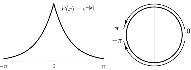
Figure 13: $F\left(x\right)=e^{-\left|x\right|}$ on $\mathbb{R}/2\pi\mathbb{Z}$

16 Example: $e^{i2\pi x}$

This is a trivial example, but it is helpful to understand subtleties of extensions of positive definite functions. In a different context, one studies classes of unbounded Hermitian operators which arise in scattering theory for wave equations in physics; see e.g., PT (13); JPT (12); LP (89, 85). For a discussion, see e.g., Section 35.1, and Lemma 35.8.

Consider the quantum mechanical momentum operator

$$P=-\frac{1}{2\pi i}\frac{d}{dx},\quad dom\left(P\right)=C_{c}^{\infty}\left(\mathbb{T}\right),$$

acting in $L^{2}\left(\mathbb{T}\right)$, where $\mathbb{T}\simeq\mathbb{R}/\mathbb{Z}\simeq\left(-\frac{1}{2},\frac{1}{2}\right]$. $P$ is Hermitian, with a dense domain in $L^{2}\left(\mathbb{T}\right)$. It has deficiency indices $\left(1,1\right)$, and the family of selfadjoint extensions is determined by the boundary condition (205).

Setting $\theta=0$ in (205), the corresponding selfadjoint (s.a.) extension $\widetilde{P}\supset P$ has spectrum

$$\sigma(\widetilde{P})=\left\{\xi_{n}:=e^{i2\pi nx}\>|\>n\in\mathbb{Z}\right\};$$

so that if $U\left(t\right)=e^{it\widetilde{P}}$, $t\in\mathbb{R}$, then $\left(U\left(t\right)f\right)\left(x\right)=f\left(x+t\right)$, for all $f\in L^{2}\left(\mathbb{T}\right)$. That is, $U\left(t\right)$ is the translation group.

Example 16.1.

Now fix $0<\epsilon<\frac{1}{2}$, and set

$$F\left(x\right):=e^{i2\pi x}\big{|}{}_{\left(-\epsilon,\epsilon\right)}.$$ (207)

Lemma 16.2.

The RKHS $\mathscr{H}_{F}$ of $F$ in (207) is one-dimensional. Moreover, for all $\varphi,\psi\in C_{c}^{\infty}\left(0,\epsilon\right)$, we have

$$\left\langle F_{\varphi},F_{\psi}\right\rangle_{\mathscr{H}_{F}}=\overline{\widehat{\varphi}\left(1\right)}\widehat{\psi}\left(1\right).$$ (208)

In particular,

$$\left\|F_{\varphi}\right\|_{\mathscr{H}_{F}}^{2}=\left|\widehat{\varphi}\left(1\right)\right|^{2}.$$ (209)

Here, $\widehat{\cdot}$ denotes Fourier transform.

Proof 16.3.

Recall that $\mathscr{H}_{F}$ is the completion of $span\left\{F_{\varphi}:\varphi\in C_{c}^{\infty}\left(0,\epsilon\right)\right\}$, where

$$F_{\varphi}\left(x\right) = \int_{0}^{\epsilon}\varphi\left(y\right)F\left(x-y\right)dy$$

$$= e^{i2\pi x}\int_{0}^{\epsilon}\varphi\left(y\right)e^{-i2\pi y}dy=e^{i2\pi x}\widehat{\varphi}\left(1\right);$$

it follows that $\dim\mathscr{H}_{F}=1$.

Moreover,

$$\left\langle F_{\varphi},F_{\psi}\right\rangle_{\mathscr{H}_{F}} = \int_{0}^{\epsilon}\int_{0}^{\epsilon}\overline{\varphi\left(x\right)}\psi\left(y\right)F\left(x-y\right)dxdy$$

$$= \overline{\widehat{\varphi}\left(1\right)}\widehat{\psi}\left(1\right),\quad\forall\varphi,\psi\in C_{c}^{\infty}\left(0,\epsilon\right);$$

which is the assertion (208).     ∎

Note that $F$ in (207) is the restriction of a p.d. function, so it has at least one extension, i.e., $e^{i2\pi x}$ on $\mathbb{T}$. In fact, this is also the unique continuous p.d. extension to $\mathbb{T}$.

Lemma 16.4.

Let $F$ be as in (207). If $\widetilde{F}$ is a continuous p.d. extension of $F$ on $\mathbb{T}$, then $\widetilde{F}\left(x\right)=e^{i2\pi x}$, $x\in\left(-\frac{1}{2},\frac{1}{2}\right]$.

Proof 16.5.

Assume $\widetilde{F}$ is a continuous p.d. extension of $F$ to $\mathbb{T}$, then by Bochner’s theorem, we have

$$e^{i2\pi x}=\sum_{n\in\mathbb{Z}}\mu_{n}e^{i2\pi nx},\quad\forall x\in\left(-\epsilon,\epsilon\right)$$ (210)

where $\mu_{n}\geq 0$, and $\sum_{n\in\mathbb{Z}}\mu_{n}=1$. Now each side of the above equation extends continuously in $x$. By uniqueness of the Fourier expansion in (210), we get $\mu_{1}=1$, and $\mu_{n}=0$, $n\in\mathbb{Z}\backslash\left\{1\right\}$.     ∎

Remark 16.6.

In fact, Lemma 16.4 holds in a more general context. (We thank the anonymous referee who kindly suggested the following abstract argument.)

Proposition 16.7.

Let $G$ be a connected locally compact Abelian group, $u$ a positive definite function on $G$ and $\chi$ a character for which $\chi|_{U}=u|_{U}$ for some neighborhood of $U$ of the origin $1$. Then $u=\chi$.

Proof 16.8.

Indeed let $v=\overline{\chi}u$ which is $1$ on $U$. An easy argument shows that then $v$ is also p.d. on $G$.

We now pass to the Gelfand-Naimark-Segal (GNS) representation (see Theorem 13.13), i.e., to a Hilbert space $\mathscr{H}$, $\sigma$ a cyclic representation of $G$ acting on $\mathscr{H}$, and a unit vector $\xi\in\mathscr{H}$ s.t. $v\left(x\right)=\left\langle\xi,\sigma\left(x\right)\xi\right\rangle_{\mathscr{H}}$, for all $x\in G$.

Notice that $H=\left\{x\in G:v(x)=1\right\}$ is a subgroup. Indeed, since $v=\langle\xi,\sigma(\cdot)\xi\rangle$ where $\|\xi\|=1$, then $H=\{x\in G:\sigma(x)\xi=\xi\}$, thanks to uniform convexity. But $H\supseteq U$ so $H\supseteq\bigcup_{n=1}^{\infty}U^{n}=G$, where we used that $G$ is assumed connected.     ∎

17 Example: $e^{-\left|x\right|}$ in $\left(-a,a\right)$, extensions to $\mathbb{T}=\mathbb{R}/\mathbb{Z}$

Fix $0<a<\frac{1}{2}$. Let $F:\Omega-\Omega\rightarrow\mathbb{C}$ be a continuous p.d. function, where $\Omega=\left(0,a\right)$.

For the extension problem (continuous, p.d.), we consider two cases:

$$\Omega\subset\mathbb{R}\quad\mbox{vs.}\quad\Omega\subset\mathbb{T}=\mathbb{R}/\mathbb{Z}$$ (211)

First, recall the Pontryagin duality (see Rud (90)) for locally compact Abelian (l.c.a) groups:

$$\Phi\left(x\right)=\int_{\widehat{G}}\chi\left(x\right)d\mu\left(\chi\right),\quad\chi\in\widehat{G},\>x\in G$$ (212)

Application: In our current setting, $G=\mathbb{T}=\mathbb{R}/\mathbb{Z}$, $\widehat{G}=\mathbb{Z}$, and

$$\chi_{n}\left(x\right)=e^{i2\pi nx},\quad n\in\mathbb{Z},\>x\in\mathbb{T};$$ (213)

so that

$$\Phi\left(x\right)=\sum_{n\in\mathbb{Z}}w_{n}e^{i2\pi nx},\quad w_{n}\geq 0,\>\sum_{n\in\mathbb{Z}}w_{n}<\infty.$$ (214)

The weights $\left\{w_{n}\right\}$ in (214) determines a measure $\mu_{w}$ on $\mathbb{Z}$, where

$$\mu_{w}\left(E\right):=\sum_{n\in E}w_{n},\quad\forall E\subset\mathbb{Z}.$$ (215)

Conclusions: Formula (214) is a special case of formula (212); and (212) is the general l.c.a. Pontryagin-Bochner duality. (If $\Phi\left(0\right)=1$, then $\mu_{w}$ is a probability measure on $\mathbb{Z}$.)

Remark 17.1.

Distributions as in (215) arise in many applications; indeed stopping times of Markov chains is a case in point Sok (13); Du (12).

Let $\left(\Omega,\mathscr{F},\mathbb{P}\right)$ be a probability space, and let $X_{n}:\Omega\rightarrow\mathbb{R}$ be a stochastic process indexed by $\mathbb{Z}$. Let $M\subset\mathbb{R}$ be a bounded Borel subset. The corresponding stopping time $\tau_{M}$ is as follows:

For $\omega\in\Omega$, set

$$\tau_{M}\left(\omega\right)=\inf\left\{n\in\mathbb{Z}\>|\>X_{n}\left(\omega\right)\in M\right\}.$$ (216)

The distribution $\mu_{\tau_{M}}$ of $\tau_{M}$ is an example of a measure on $\mathbb{Z}$, i.e., an instance of the setting in (215).

For $n\in\mathbb{Z}$, set

$$w_{n}^{M}:=\mathbb{P}\left(\left\{\omega\in\Omega\>|\>\tau_{M}\left(\omega\right)=n\right\}\right),\quad n\in\mathbb{Z}.$$

Assume that the values of $\tau_{M}$ are finite so $\tau_{M}:\Omega\rightarrow\mathbb{Z}$. Then it follows from the definition of stopping time (216) that $w_{n}^{M}\geq 0$, $\forall n\in\mathbb{Z}$; and $\sum_{n\in\mathbb{Z}}w_{n}^{M}=1$.

Back to the extension problem (211). In fact, there are many more solutions to the $\mathbb{R}$-problem than periodic solutions on $\mathbb{T}$. By the Pontryagin duality (see Rud (90)), any periodic solution $\widetilde{F}_{per}$ has the representation (214).

Example 17.2 (The periodic extension continued).

Recall that $e^{-\left|x\right|}$, $x\in\mathbb{R}$, is positive definite on $\mathbb{R}$, where

$$e^{-\left|x\right|}=\int_{-\infty}^{\infty}\frac{2}{1+4\pi^{2}\lambda^{2}}e^{i2\pi\lambda x}d\lambda,\quad x\in\mathbb{R}.$$ (217)

By the Poisson summation formula, we have:

$$\begin{split}\widetilde{F}_{per}\left(x\right)&=\sum_{n\in\mathbb{Z}}e^{-\left|x-n\right|}=\sum_{n\in\mathbb{Z}}w_{n}e^{i2\pi nx}\\ w_{n}&=\frac{2}{1+4\pi^{2}n^{2}}\end{split}$$ (218)

$\widetilde{F}_{per}\left(x\right)$ is a continuous p.d. function on $\mathbb{T}$; and obviously, an extension of the restriction $\widetilde{F}_{per}\big{|}_{\left(-a,a\right)}$. Note that

$$\sum_{n\in\mathbb{Z}}w_{n}=\sum_{n\in\mathbb{Z}}\frac{2}{1+4\pi^{2}n^{2}}=\coth\left(1/2\right)<\infty.$$ (219)

General Consideration

There is a bijection between (i) functions on $\mathbb{T}$, and (ii) $1$-periodic functions on $\mathbb{R}$. Note that (ii) includes p.d. functions $F$ defined only on a subset $\left(-a,a\right)\subset\mathbb{T}$.

Given $0<a<\frac{1}{2}$, if $F$ is continuous and p.d. on $\left(-a,a\right)\subset\mathbb{T}$, then the analysis of the corresponding RKHS $\mathscr{H}_{F}$ is totally independent of considerations of periods. $\mathscr{H}_{F}$ does not see global properties. To understand $F$ on $\left(-a,a\right)$, only one period interval is needed; but when passing to $\mathbb{R}$, things can be complicated. Hence, it is tricky to get extensions $\widetilde{F}_{per}$ to $\mathbb{T}$.

Example 17.3.

Let $F\left(x\right)=e^{-\left|x\right|}$, for all $x\in\left(-a,a\right)$. See Figure 14. Then $\widetilde{F}\left(x\right)=e^{-\left|x\right|}$, $x\in\mathbb{R}$, is a continuous p.d. extension to $\mathbb{R}$. However, the periodic version in (218) is NOT a p.d. extension of $F$. See Figure 15.

Note this bijection also applies if a continuous p.d. function $F$ is only defined on a subset $\left(-a,a\right)\subset\mathbb{T}$, with $0<a<\frac{1}{2}$.

Figure 14: Functions on $\mathbb{T}=\mathbb{R}/\mathbb{Z}\longleftrightarrow$ $\bigl{(}\mbox{1-periodic functions on $\mathbb{R}$ }\bigr{)}$.

Figure 15: $\widetilde{F}_{per}\left(x\right)>F\left(x\right)$ on $\left[-\frac{1}{2},\frac{1}{2}\right]$

Example 17.4.

Fix $a\in\left(0,\frac{1}{2}\right)$. Let $F\left(x\right)=e^{-\left|x\right|}$, $x\in\left(-a,a\right)$. Note that

$$\left(e^{-\left|\cdot\right|}\chi_{\left[-\frac{1}{2},\frac{1}{2}\right]}\right)^{\wedge}\left(\lambda\right) = \int_{\mathbb{R}}\frac{\sin\pi\left(\lambda-t\right)}{\pi\left(\lambda-t\right)}\cdot\frac{2}{1+4\pi^{2}t^{2}}dt$$ (220)

$$= \frac{2\left(2\pi\lambda\sin(\pi\lambda)-\cos(\pi\lambda)+\sqrt{e}\right)}{\sqrt{e}\left(1+4\pi^{2}\lambda^{2}\right)},$$

then, using Shannon’s interpolation formula, we get

$$\widetilde{F}_{cir}\left(x\right) := \sum_{n\in\mathbb{Z}}e^{-\left|x+n\right|}\chi_{\left[-\frac{1}{2},\frac{1}{2}\right]}\left(x+n\right)=\sum_{n\in\mathbb{Z}}\widehat{W}\left(n\right)e^{i2\pi nx};\;\mbox{where}$$ (221)

$$\widehat{W}\left(n\right) :=\left(e^{-\left|\cdot\right|}\chi_{\left[-\frac{1}{2},\frac{1}{2}\right]}\right)^{\wedge}\left(n\right)\overset{\text{$\left(\ref{eq:FperW}\right)$}}{=} \frac{2\left(1-e^{-1/2}\left(-1\right)^{n}\right)}{1+4\pi^{2}n^{2}},\quad\forall n\in\mathbb{Z}.$$ (222)

See Figures 16-17.

It follows from (217)-(218), that

$$\sum_{n\in\mathbb{Z}}\widehat{W}\left(n\right) = \sum_{n\in\mathbb{Z}}e^{-\left|n\right|}-e^{-1/2}\sum_{n\in\mathbb{Z}}e^{-\left|n-\frac{1}{2}\right|}=1,\;\mbox{and}$$

$$\widehat{W}\left(n\right) > 0,\quad\forall n\in\mathbb{Z}.$$

Therefore, the weights $\{\widehat{W}\left(n\right)\}$ in (222) determines a probability measure on $\mathbb{Z}$ (using the normalization $F\left(0\right)=1$.) By Bochner’s theorem, $\widetilde{F}_{cir}$ in (221) is a continuous p.d. extension of $F$, thus a solution to the $\mathbb{T}$-problem.

Figure 16: A p.d. extension from $F$ to $\widetilde{F}_{cir}$ defined on $\mathbb{T}$.

Set $\widehat{W}\left(\lambda\right):=\left(e^{-\left|\cdot\right|}\chi_{\left(-1/2,1/2\right)}\right)^{\wedge}\left(\lambda\right)$, then $\{\widehat{W}\left(n\right)\}_{n\in\mathbb{Z}}$ is a probability distribution on $\mathbb{Z}$.

Figure 17: A periodic extension of $e^{-\left|\cdot\right|}\chi_{\left[-1/2,1/2\right]}$ on $\mathbb{R}$ by Shannon’s interpolation.

Example 17.5.

Fix $0<a<\frac{1}{2}$, let $F\left(x\right)=1-\left|x\right|$, $x\in\left(-a,a\right)$, a locally defined p.d. function. This is another interesting example that we will study in Chapter 5.

Using the method from Example 17.3, we have

$$\widehat{W}\left(\lambda\right):=\left(\left(1-\left|\cdot\right|\right)\chi_{\left[-\frac{1}{2},\frac{1}{2}\right]}\right)^{\wedge}\left(\lambda\right)=\frac{\pi\lambda\sin(\pi\lambda)-\cos(\pi\lambda)+1}{2\pi^{2}\lambda^{2}}$$

and so

$$\widetilde{F}_{cir}\left(x\right):=\sum_{n\in\mathbb{Z}}\left(1-\left|x+n\right|\right)\chi_{\left[-\frac{1}{2},\frac{1}{2}\right]}\left(x+n\right)=\sum_{n\in\mathbb{Z}}\widehat{W}\left(n\right)e^{i2\pi nx},$$

where

$$\widehat{W}\left(n\right)=\frac{1-\left(-1\right)^{n}}{2\pi^{2}\lambda^{2}}\geq 0,\;\forall n\in\mathbb{Z},\;\mbox{and }\sum_{n\in\mathbb{Z}}\widehat{W}\left(n\right)=1.$$

Therefore, $\widetilde{F}_{cir}$ is a periodic p.d. extension of $F$.

Remark 17.6.

The method used in Examples 17.4-17.5 does not hold in general. For example, a periodization of the restricted Gaussian distribution, $e^{-x^{2}/2}\chi_{\left[-\frac{1}{2},\frac{1}{2}\right]}$, is not positive definite on $\mathbb{R}$. The reason is that the sampling

$$\left\{\left(e^{-\left(\cdot\right)^{2}/2}\chi_{\left[-\frac{1}{2},\frac{1}{2}\right]}\right)^{\wedge}\left(n\right)\right\}_{n\in\mathbb{Z}}$$

does NOT give a positive measure on $\mathbb{Z}$.

18 Example: $e^{-\left|x\right|}$ in $\left(-a,a\right)$, extensions to $\mathbb{R}$

In this section, we consider the following partially defined p.d. function:

$$F\left(x\right)=e^{-\left|x\right|},\quad x\in\left(-a,a\right)$$ (223)

where $0<a<\infty$, fixed. It is the restriction of

$$\begin{split}e^{-\left|x\right|}&=\int_{\mathbb{R}}e^{i\lambda x}d\mu\left(\lambda\right),\quad x\in\mathbb{R},\;\mbox{with}\\ d\mu&=\frac{d\lambda}{\pi\left(1+\lambda^{2}\right)}\left(=\mbox{prob. measure}\right),\end{split}$$ (224)

thus, $\mu\in Ext\left(F\right)$. (In particular, $Ext\left(F\right)\neq\emptyset$.)

Remark 18.1.

This special case is enlightening in connection with deficiency indices considerations. In general, there is a host of other interesting 1D examples (Chapters 5-6), some have indices $\left(1,1\right)$ and others $\left(0,0\right)$. In case of indices $\left(1,1\right)$, the convex set $Ext\left(F\right)$ is parameterized by $\mathbb{T}$; while, in case of $\left(0,0\right)$, $Ext(F)$ is a singleton. Further spectral theoretic results are given in Chapter 10, and we obtain a spectral classification of all Hermitian operators with dense domain in a separable Hilbert space, having deficiency indices $\left(1,1\right)$.

Now define $D^{\left(F\right)}$ (the canonical skew-Hermitian operator), by $D^{\left(F\right)}F_{\varphi}=F_{\varphi^{\prime}}$, with $dom(D^{\left(F\right)})=\left\{F_{\varphi}:\varphi\in C_{c}^{\infty}\left(0,a\right)\right\}$. We show below that $D^{\left(F\right)}$ has deficiency indices $\left(1,1\right)$.

Let $\mu\in Ext\left(F\right)$ be as in (224). By Corollary 12.15, there is an isometry $\mathscr{H}_{F}\hookrightarrow L^{2}\left(\mu\right)$, determined by

$$\mathscr{H}_{F}\ni F_{\varphi}\longmapsto\hat{\varphi}\in L^{2}\left(\mu\right),$$

where $\mathscr{H}_{F}$ is the corresponding RKHS. Indeed, we have

$$\left\|F_{\varphi}\right\|_{\mathscr{H}_{F}}^{2} = \int_{0}^{a}\int_{0}^{a}\overline{\varphi\left(x\right)}\varphi\left(y\right)F\left(x-y\right)dxdy$$

$$= \int_{0}^{a}\int_{0}^{a}\overline{\varphi\left(x\right)}\varphi\left(y\right)\left(\int_{\mathbb{R}}e^{i\lambda\left(x-y\right)}d\mu\right)dxdy$$

$$\overset{\text{Fubini}}{=} \int_{\mathbb{R}}\left|\widehat{\varphi}\left(\lambda\right)\right|^{2}d\mu\left(\lambda\right)=\left\|\widehat{\varphi}\right\|_{L^{2}\left(\mu\right)}^{2},\quad\forall F_{\varphi}\in dom(D^{\left(F\right)}).$$

Lemma 18.2.

Fix $0<a<\infty$, and let $F$ be a continuous p.d. function on $\left(-a,a\right)$; assume $F\left(0\right)=1$. Pick $\mu\in Ext\left(F\right)$, i.e., a probability measure on $\mathbb{R}$ s.t.

$$F\left(x\right)=\widehat{d\mu}\left(x\right),\quad\forall x\in\left(-a,a\right).$$ (225)

(We know that $Ext\left(F\right)\neq\emptyset$ from Section 7.) Then, $D^{\left(F\right)}$ has deficiency indices $\left(1,1\right)$ if and only if

$$\left(e^{\pm\left(\cdot\right)}\chi_{\left(0,a\right)}\right)^{\wedge}\left(\cdot\right)\in L^{2}\left(\mu\right).$$

$$\int_{-\infty}^{\infty}\frac{e^{2a}+1-2e^{a}\cos\left(\lambda a\right)}{1+\lambda^{2}}d\mu\left(\lambda\right)<\infty.$$ (226)

Proof 18.3.

Recall the defect vectors of $D^{\left(F\right)}$ are multiples of $e^{\pm x}$, $x\in\left(0,a\right)$. The assertion follows from the isometry $\mathscr{H}_{F}\hookrightarrow L^{2}\left(\mu\right)$.     ∎

Corollary 18.4.

Let $F$ be as in (223), then the associated $D^{\left(F\right)}$ has deficiency indices $\left(1,1\right)$. In particular, the defect vectors $\xi_{+}=e^{-x}$, $\xi_{-}=e^{a-x}$, $x\in\left(0,a\right)$, satisfy $\left\|\xi_{-}\right\|_{\mathscr{H}_{F}}=\left\|\xi_{+}\right\|_{\mathscr{H}_{F}}=1$.

Lemma 18.5.

We have:

$$\left|\left(\chi_{\left(0,a\right)}\left(x\right)e^{x}\right)^{\wedge}\left(\lambda\right)\right|^{2}=\frac{e^{2a}+1-2e^{a}\cos\left(\lambda a\right)}{1+\lambda^{2}}\;\left(\in L^{2}\left(\mathbb{R},d\lambda\right)\right),$$ (227)

where $d\lambda$ denotes the Lebesgue measure on $\mathbb{R}$.

Proof 18.6.

Direct calculation shows that

$$\left(\chi_{\left(0,a\right)}\left(x\right)e^{x}\right)^{\wedge}\left(\lambda\right)=\int_{0}^{a}e^{-i\lambda x}e^{x}dx=\frac{e^{\left(1-i\lambda\right)a}-1}{1-i\lambda};$$

which is the assertion in (227).     ∎

Now return to the RKHS $\mathscr{H}_{F}$, defined from the function $F$ in (223). Recall that $span\left\{F_{\varphi}\>\big{|}\>\varphi\in C_{c}^{\infty}\left(0,a\right)\right\}$ is a dense subspace in $\mathscr{H}_{F}$ (Lemma 7.6), where

$$F_{\varphi}\left(x\right)=\int_{0}^{a}\varphi\left(y\right)e^{-\left|x-y\right|}dy$$ (228)

Lemma 18.7.

We have

$$\left\|F_{\varphi}\right\|_{\mathscr{H}_{F}}^{2} = \int_{0}^{a}\int_{0}^{a}\overline{\varphi\left(y\right)}\varphi\left(x\right)e^{-\left|x-y\right|}dxdy$$ (229)

$$= \int_{-\infty}^{\infty}\left|\widehat{\varphi}\left(\lambda\right)\right|^{2}\frac{d\lambda}{\pi\left(1+\lambda^{2}\right)}$$

Proof 18.8.

Immediate.     ∎

Lemma 18.9 (continuation of Example 7.11).

Fix $a$, $0<a<\infty$, and let $F\left(\cdot\right):=e^{-\left|\cdot\right|}\big{|}_{\left(-a,a\right)}$ as in (223). For all $0\leq x_{0}\leq a$, let

$$F_{x_{0}}\left(x\right):=F\left(x-x_{0}\right)\Big{|}_{\left(0,a\right)}\left(\in C\left(0,a\right)\right).$$ (230)

With

$$DEF^{+} =\left\{\xi:\bigl{(}D^{\left(F\right)}\bigr{)}^{*}\xi=\xi\right\}=span\left\{\xi_{+}\left(x\right):=e^{-x}\Big{|}_{\left(0,a\right)}\right\}$$ (231)

$$DEF^{-} =\left\{\xi:\bigl{(}D^{\left(F\right)}\bigr{)}^{*}\xi=-\xi\right\}=span\left\{\xi_{-}\left(x\right):=e^{-a}e^{+x}\Big{|}_{\left(0,a\right)}\right\}$$ (232)

we get

$$\left\|\xi_{+}\right\|_{\mathscr{H}_{F}}^{2}=\left\|\xi_{-}\right\|_{\mathscr{H}_{F}}^{2}=1.$$ (233)

Proof 18.10.

Note that $x=0$ and $x=a$ are the endpoints in the open interval $\left(0,a\right)$:

$$\xi_{+}\left(x\right) =e^{-x}\Big{|}_{\left(0,a\right)}=F_{0}\left(x\right)$$

$$\xi_{-}\left(x\right) =e^{-a}e^{x}\Big{|}_{\left(0,a\right)}=F_{a}\left(x\right).$$

Let $\psi_{n}\in C_{c}^{\infty}\left(0,a\right)$ be an approximate identity, such that

1. $\psi_{n}\geq 0$, $\int\psi_{n}=1$;

2. $\psi_{n}\rightarrow\delta_{a}$, as $n\rightarrow\infty$.

Then

$$\xi_{-}\left(x\right)=F_{a}\left(x\right)=\lim_{n\rightarrow\infty}\int_{0}^{a}\psi_{n}\left(y\right)F_{y}\left(x\right)dy.$$

This shows that $\xi_{-}\in\mathscr{H}_{F}$. Also,

$$\left\|\xi_{-}\right\|_{\mathscr{H}_{F}}^{2} = \left\|F_{a}\right\|_{\mathscr{H}_{F}}^{2}$$

$$= \lim_{n\rightarrow\infty}\frac{1}{2\pi}\int_{-\infty}^{\infty}\left|\widehat{\psi_{n}}\left(y\right)\right|^{2}\widehat{F}\left(y\right)dy$$

$$= \frac{1}{2\pi}\int_{-\infty}^{\infty}\widehat{F}\left(y\right)dy=1.$$

Similarly, if instead, $\psi_{n}\rightarrow\delta_{0}$, then

$$\xi_{+}\left(x\right)=F_{0}\left(x\right)=\lim_{n\rightarrow\infty}\int_{0}^{a}\psi_{n}\left(y\right)F_{y}\left(x\right)dy$$

and $\left\|\xi_{+}\right\|_{\mathscr{H}_{F}}^{2}=1$.

∎

Lemma 18.11.

Let $F$ be as in (223). We have the following for its Fourier transform:

$$\widehat{F}\left(y\right)=\frac{2-2e^{-a}\left(\cos\left(ay\right)-y\sin\left(ay\right)\right)}{1+y^{2}}.$$

Proof 18.12.

Let $y\in\mathbb{R}$, then

$$\widehat{F}\left(y\right) = \int_{-a}^{a}e^{iyx}e^{-\left|x\right|}dx$$

$$= \int_{-a}^{0}e^{iyx}e^{x}dx+\int_{0}^{a}e^{iyx}e^{-x}dx$$

$$= \frac{1-e^{-a(1+iy)}}{1+iy}+\frac{e^{ia(y+i)}-1}{-1+iy}$$

$$= \frac{2-2e^{-a}\left(\cos\left(ay\right)-y\sin\left(ay\right)\right)}{1+y^{2}}$$

which is the assertion.     ∎

Remark 18.13.

If $\left(F,\Omega\right)$ is such that $D^{\left(F\right)}$ has deficiency indices $\left(1,1\right)$, then by von Neumann’s theory DS (88), the family of selfadjoint extensions is characterized by

$$dom\left(A_{\theta}^{\left(F\right)}\right) =\left\{F_{\psi}+c\left(\xi_{+}+e^{i\theta}\xi_{-}\right):\psi\in C_{c}^{\infty}\left(0,a\right),c\in\mathbb{C}\right\}$$

$$A_{\theta}^{\left(F\right)}: F_{\psi}+c\left(\xi_{+}+e^{i\theta}\xi_{-}\right)\mapsto F_{i\psi^{\prime}}+c\,i\left(\xi_{+}-e^{i\theta}\xi_{-}\right),\mbox{ where }i=\sqrt{-1}.$$

Proposition 18.14.

Let $F\left(x\right)=e^{-\left|x\right|}$, $x\in\left(-a,a\right)$, be the locally defined p.d. function (see (223)), and $\mathscr{H}_{F}$ be the associated RKHS. Consider $e_{\lambda}\left(x\right)=\chi_{\left(0,a\right)}\left(x\right)e^{i\lambda x}$ with $\lambda\in\mathbb{C}$ fixed. Then the function $e_{\lambda}\in\mathscr{H}_{F}$, for all $\lambda\in\mathbb{C}$.

Proof 18.15.

For simplicity, set $a=1$. Fix $\lambda\in\mathbb{C}$, and consider two cases:

Case 1. $\Im\left\{\lambda\right\}=0$, i.e. , $\lambda\in\mathbb{R}$.

Recall the isometry $T:\mathscr{H}_{F}\rightarrow L^{2}\left(\mu\right)$, with $d\mu$ as in (224); and by Corollary 14.5, the adjoint operator is given by

$$L^{2}\left(\mu\right)\ni f\xrightarrow{\quad T^{*}\;}\chi_{\left[0,1\right]}\left(fd\mu\right)^{\vee}\in\mathscr{H}_{F}.$$

We shall show that there exists $f\in L^{2}\left(\mu\right)$ s.t. $T^{*}f=\chi_{\left[0,1\right]}e_{\lambda}$.

Let

$$\varphi\left(x\right) = \left(\chi_{\left[-1,1\right]}*\chi_{\left[0,1\right]}\right)\left(x\right)$$ (234)

$$= \left|\left[x-1,x\right]\cap\left[-1,1\right]\right|,\quad x\in\mathbb{R},$$

where $\left|\cdots\right|$ denotes Lebesgue measure. See Figure 18. Note that

$$\widehat{\varphi}\left(t\right) = \frac{2\sin(t)}{t}\cdot\frac{2\sin\left(t/2\right)}{t}e^{-it/2}$$ (235)

$$\left|\widehat{\varphi}\left(t\right)\right|^{2} = \frac{16\sin^{2}\left(t\right)\sin^{2}\left(t/2\right)}{t^{4}},\quad t\in\mathbb{R}.$$ (236)

Now, set $e_{\lambda}\left(x\right):=e^{i\lambda x}$, and

$$\psi\left(x\right) = e_{\lambda}\left(x\right)\varphi\left(x\right),\;\mbox{and}$$ (237)

$$f\left(t\right) = \frac{1}{2}\widehat{\psi}\left(t\right)\left(1+t^{2}\right),\quad t\in\mathbb{R}.$$ (238)

Then, we have:

$$\left(T^{*}f\right)\left(x\right) = \left(\chi_{\left[0,1\right]}\left(fd\mu\right)^{\vee}\right)\left(x\right)$$

$$= \chi_{\left[0,1\right]}\left(x\right)\int_{\mathbb{R}}e^{itx}\frac{1}{2}\hat{\psi}\left(t\right)\left(1+t^{2}\right)\frac{dt}{\pi\left(1+t^{2}\right)}$$

$$= \chi_{\left[0,1\right]}\left(x\right)\frac{1}{2\pi}\int_{\mathbb{R}}e^{itx}\widehat{\psi}\left(t\right)dt$$

$$= \chi_{\left[0,1\right]}\left(x\right)\psi\left(x\right)=\chi_{\left[0,1\right]}\left(x\right)e_{\lambda}\left(x\right);\;\mbox{and}$$

$$\int_{\mathbb{R}}\left|f\right|^{2}d\mu = \frac{1}{4}\int_{\mathbb{R}}\left|\hat{\psi}\left(t\right)\right|^{2}\left(1+t^{2}\right)^{2}\frac{1}{\pi\left(1+t^{2}\right)}dt$$

$$= \frac{1}{4\pi}\int_{\mathbb{R}}\left|\hat{\psi}\left(t\right)\right|^{2}\left(1+t^{2}\right)dt$$

$$= \frac{4}{\pi^{2}}\int_{\mathbb{R}}\frac{\sin^{2}\left(\left(t-\lambda\right)/2\right)\sin^{2}\left(t-\lambda\right)}{\left(t-\lambda\right)^{4}}\left(1+t^{2}\right)dt<\infty.$$

Thus, the function $f$ in (238) is in $L^{2}\left(\mu\right)$, and satisfies $T^{*}f=\chi_{\left[0,1\right]}e_{\lambda}$. This is the desired conclusion.

Case 2. $\Im\left\{\lambda\right\}\neq 0$.

Using general theory DS (88), it is enough to prove that $e_{\lambda}\left(x\right)$ is in $\mathscr{H}_{F}$ for $\lambda=\pm i$. So consider the following:

$$\begin{split}\xi_{+}\left(x\right)&=e^{-x}\chi_{\left(0,1\right)}\left(x\right)\\ \xi_{-}\left(x\right)&=e^{x-1}\chi_{\left(0,1\right)}\left(x\right).\end{split}$$ (239)

Let $S$ be the isometry in Corollary 7.10, then

$$S^{*}\underset{\in\mathscr{H}_{F}}{\underbrace{\left(\nu*F\right)}}=\nu\in\mathfrak{M}_{2}\left(F\right)$$ (240)

for all signed measures $\nu\in\mathfrak{M}_{2}\left(F\right)$. Fixing $\mu$ positive s.t. $\widehat{d\mu}\left(x\right)=F\left(x\right)$ for all $x\in\left[-1,1\right]$, we get

$$\nu*F\in\mathscr{H}_{F}\Longleftrightarrow\int_{\mathbb{R}}\left|\widehat{\nu}\left(t\right)\right|^{2}d\mu\left(t\right)<\infty,$$

and

$$\left\|\nu*F\right\|_{\mathscr{H}_{F}}^{2}=\int_{\mathbb{R}}\left|\widehat{\nu}\left(t\right)\right|^{2}d\mu\left(t\right).$$ (241)

Here, $\left(\nu*F\right)\left(x\right)=\int_{0}^{1}F\left(x-y\right)d\nu\left(y\right)$, $\forall x\in\left[0,1\right]$.

In Example 7.11, we proved that

$$\begin{split}\left(\delta_{0}*F\right)\left(x\right)&=\xi_{+}\left(x\right)\\ \left(\delta_{1}*F\right)\left(x\right)&=\xi_{-}\left(x\right)\end{split}$$ (242)

Using (241), we then get

$$\left\|\xi_{+}\right\|_{\mathscr{H}_{F}}^{2}=\|\widehat{\delta_{0}}\|_{L^{2}\left(\mathbb{R},\mu\right)}^{2}=1$$

and

$$\left\|\xi_{-}\right\|_{\mathscr{H}_{F}}^{2}=\|\widehat{\delta_{1}}\|_{L^{2}\left(\mathbb{R},\mu\right)}^{2}=1;$$

where of course $\widehat{\delta_{0}}\equiv 1$, $\forall t\in\mathbb{R}$, and $\widehat{\delta_{1}}=e^{it}$.     ∎

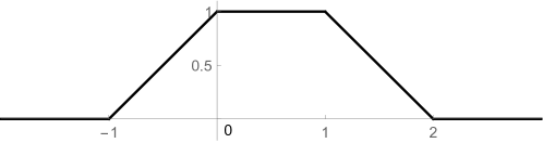
Figure 18: Convolution product $\varphi=\chi_{\left[0,1\right]}*\chi_{\left[-1,1\right]}$ from (234).

Remark 18.16.

In Tables 1-2, we consider six examples of locally defined continuous p.d. functions, all come from restrictions of p.d. functions on $\mathbb{R}$. Except for the trivial case $F_{6}$, for each $F_{j}$, $j=1,\dots,5$, we need to decide whether $e_{\lambda}\left(x\right)=e^{i\lambda x}$, $\lambda\in\mathbb{C}$, are in the corresponding RKHS $\mathscr{H}_{F_{j}}$.

For illustration, it suffices to consider the case $\lambda=0$, i.e., whether the constant functions $\chi_{\left[0,a\right]}$ are in $\mathscr{H}_{F_{j}}$. Equivalently, if there exists $f\in L^{2}(\mu)$, s.t.

$$\varphi = T^{*}f=\chi_{\left[0,a\right]}\left(fd\mu\right)^{\vee},\;\mbox{s.t.}$$ (243)

$$\varphi \equiv 1\;\mbox{on }\left[0,a\right].$$ (244)

Here, $d\mu$ denotes one of the measures introduced above. Compare with Proposition 18.14.

Note that in all cases, $d\mu$ is absolutely continuous w.r.t. the Lebesgue measure, i.e., $d\mu=m\>dx$, where $m$ is a Radon-Nikodym derivative. Thus, a possible solution $f$ to (243)-(244) must be given by

$$\widehat{f}=\frac{\widehat{\varphi}}{m},\quad\mbox{s.t.}\quad\int_{\mathbb{R}}\frac{\left|\widehat{\varphi}\right|^{2}\left(t\right)}{m\left(t\right)}dt<\infty.$$ (245)

By the splitting, $\varphi=\varphi\chi_{\left[0,a\right]}+\varphi_{2}$, and using (244), we then get

$$\widehat{\varphi}\left(t\right)=\mbox{sinc}\left(t\right)+\widehat{\varphi}_{2}\left(t\right),$$ (246)

where, in (246), we use that $\varphi_{2}$ is supported in $\mathbb{R}\backslash\left(0,a\right)$. In the applications mentioned above, the sinc function in (246) will already account for the divergence of the integral in (245).

Conclusion: One checks that for $F_{1},F_{4}$, and $F_{5}$, the function $\chi_{\left[0,a\right]}$ is not in the corresponding RKHS.

Example 18.17.

$F_{1}\left(x\right)=\frac{1}{1+x^{2}}$, $\left|x\right|<1$, $d\mu_{1}\left(t\right)=\frac{1}{2}e^{-\left|t\right|}dt$. Then, we have

$$\int_{\mathbb{R}}\frac{\left|\widehat{\varphi}\right|^{2}\left(t\right)}{m\left(t\right)}dt\sim\int_{\mathbb{R}}\mbox{sinc}^{2}\left(t\right)e^{\left|t\right|}dt+\mbox{other positive terms}$$

which is divergent. Thus, $\chi_{\left[0,1\right]}\notin\mathscr{H}_{F_{1}}$.

Remark 18.18.

In the example above, we cannot have

$$\left|\widehat{\varphi}\right|^{2}\left(t\right)\sim O(e^{-\left(1+\epsilon\right)\left|t\right|}),\;\mbox{as }\left|t\right|\rightarrow\infty;$$ (247)

for some $\epsilon>0$. Should (247) hold, then By the Paley-Wiener theorem, $x\mapsto\varphi\left(x\right)$ would have an analytic continuation to a strap, $\left|\Im z\right|<\alpha$, $z=x+iy$, $\left|y\right|<\alpha$. But this contradicts the assumption that $\varphi\left(x\right)\equiv 1$, for all $x\in\left(0,1\right)$; see (244).

If people do not believe that mathematics is simple, it is only because they do not realize how complicated life is.
— John von Neumann

19 Example: A non-extendable p.d. function in a neighborhood of zero in $G=\mathbb{R}^{2}$

Let $M$ denote the Riemann surface of the complex $\log z$ function. $M$ is realized as a covering space for $\mathbb{R}^{2}\backslash\left\{\left(0,0\right)\right\}$ with an infinite number of sheets indexed by $\mathbb{Z}$, see Figure 19.

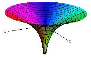
Figure 19: $M$ the Riemann surface of $\log z$ as an $\infty$ cover of $\mathbb{R}^{2}\backslash\left\{\left(0,0\right)\right\}$.

The 2D-Lebesgue measure lifts to a unique measure on $M$; hence $L^{2}\left(M\right)$. Here the two skew-symmetric operators $\frac{\partial}{\partial x_{j}}$, $j=1,2$, with domain $C_{c}^{\infty}\left(M\right)$ define an Abelian 2-dimensional Lie algebra of densely defined operators in the Hilbert space $L^{2}\left(M\right)$.

Proposition 19.1.

1. Each operator $\frac{\partial}{\partial x_{j}}$, defined on $C_{c}^{\infty}\left(M\right)$, is essentially skew-adjoint in $L^{2}\left(M\right)$, i.e.,

   $$-\left(\frac{\partial}{\partial x_{j}}\Big{|}_{C_{c}^{\infty}\left(M\right)}\right)^{*}=\overline{\frac{\partial}{\partial x_{j}}\Big{|}_{C_{c}^{\infty}\left(M\right)}},\quad j=1,2;$$ (248)

   where the r.h.s. in (248) denotes operator closure.

2. The $\left\{\frac{\partial}{\partial x_{j}}\right\}_{j=1,2}$ Lie algebra with domain $C_{c}^{\infty}\left(M\right)\subset L^{2}\left(M\right)$ does not extend to a unitary representation of $G=\mathbb{R}^{2}$.

3. The two skew-adjoint operators in (248) are NOT strongly commuting.

4. The Laplace operator

   $$L:=\left(\frac{\partial}{\partial x_{1}}\right)^{2}+\left(\frac{\partial}{\partial x_{2}}\right)^{2},\quad dom\left(L\right)=C_{c}^{\infty}\left(M\right)$$ (249)

   has deficiency indices $\left(\infty,\infty\right)$.

Proof 19.2.

For $j=1,2$, the operators $\frac{\partial}{\partial x_{j}}\big{|}_{C_{c}^{\infty}\left(M\right)}$ generate unitary one-parameter groups $U_{j}\left(t\right)$ on $L^{2}\left(M\right)$, lifted from the coordinate translations:

$$\left(x_{1},x_{2}\right) \longmapsto \left(x_{1}+s,x_{2}\right),\quad x_{2}\neq 0$$ (250)

$$\left(x_{1},x_{2}\right) \longmapsto \left(x_{1},x_{2}+t\right),\quad x_{1}\neq 0$$ (251)

It is immediate that the respective infinitesimal generators are the closed operators $\overline{\frac{\partial}{\partial x_{j}}\big{|}_{C_{c}^{\infty}\left(M\right)}}$. Part (1) follows from this.

Part (2)-(4). Suppose $\varphi\in C_{c}^{\infty}\left(M\right)$ is supported over some open set in $\mathbb{R}^{2}\backslash\left\{\left(0,0\right)\right\}$, for example, $\left(x_{1}-2\right)^{2}+x_{2}^{2}<1$. If $1<s,t<2$, then the functions

$$U_{1}\left(s\right)U_{2}\left(t\right)\varphi\quad\mbox{vs.}\quad U_{2}\left(t\right)U_{1}\left(s\right)\varphi$$ (252)

are supported on two opposite levels in the covering space $M$; see Figure 20. (One is over the other; the two are on “different floors of the parking garage.”) Hence the unitary groups $U_{j}\left(t\right)$ do not commute. It follows from Nelson’s theorem Nel (59) that $L$ in (249) is not essentially selfadjoint, equivalently, the two skew-adjoint operators are not strongly commuting.

Since $L\leq 0$ (in the sense of Hermitian operators), so it has equal deficiency indices. In fact, $L$ has indices $\left(\infty,\infty\right)$; see JT14a ; Tia (11).

This completes the proof of the proposition.     ∎

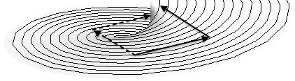
Figure 20: Translation of $\varphi$ to different sheets.

Remark 19.3.

The two unitary groups from Proposition 19.1 define a local representation of $G=\mathbb{R}^{2}$ on $L^{2}\left(M\right)$, but not a global one. That is, the skew-adjoint operators $\overline{\frac{\partial}{\partial x_{j}}\big{|}_{C_{c}^{\infty}\left(M\right)}}$ in (248) are not strongly commuting, and so

$$\rho:\left(s,t\right)\longmapsto U_{1}\left(s\right)U_{2}\left(t\right)$$ (253)

is not a unitary representation of $\mathbb{R}^{2}$ on $L^{2}\left(M\right)$. This is different from the 1D examples.

The harmonic analysis of the Riemann surface $M$ of $\log z$ is of independent interest, but it will involve von Neumann algebras and non-commutative geometry. Note that to study this, one is faced with two non-commuting unitary one-parameter groups acting on $L^{2}\left(M\right)$ (corresponding to the two coordinates for $M$). Of interest here is the von Neumann algebra generated by these two non-commuting unitary one-parameter groups. It is likely that this von Neumann algebra is a type III factor. There is a sequence of interesting papers by K. Schmudgen on dealing with some of this Sch (84); SF (84); Sch (85); Sch86b ; Sch86a .

A locally defined p.d. functions $F$ on $G=\mathbb{R}^{2}$ with $Ext\left(F\right)=\emptyset$.

Let $M$ be the Riemann surface of the complex $\log z$; see Figure 19.

Denote $B_{r}\left(x\right):=\left\{y\in\mathbb{R}^{2}\>:\>\left|x-y\right|<r,\;r>0\right\}$, $x\in\mathbb{R}^{2}$, the open neighborhood of points $x\in\mathbb{R}^{2}$ of radius $r$. Pick $\xi\in C_{c}^{\infty}\left(B_{1/2}\left(1,1\right)\right)$, such that

$$\iint\xi=1,\quad\xi\geq 0.$$ (254)

Note that $\xi$ is supported on level 1 of the covering surface $M$, i.e., on the sheet $\mathbb{R}^{2}\backslash\left\{\left(x,y\right):x\geq 0\right\}$; assuming the branch cuts are along the positive $x$-axis.

Let $\pi:M\rightarrow\mathbb{R}^{2}\backslash\left\{0\right\}$ be the covering mapping. Set

$$\left(\sigma\left(t\right)\xi\right)\left(m\right):=\xi\left(\pi^{-1}\left(t+\pi\left(m\right)\right)\right),\quad\forall t\in B_{1/2}\left(0\right),\;\forall m\in M.$$ (255)

Lemma 19.4.

The function

$$F\left(t\right):=\left\langle\xi,\sigma\left(t\right)\xi\right\rangle_{L^{2}\left(M\right)},\quad t\in B_{1/2}\left(0\right)\subset\mathbb{R}^{2}$$ (256)

is defined on a local neighborhood of $0\in\mathbb{R}^{2}$, continuous and p.d.; but cannot be extended to a continuous p.d. function $F^{ext}$ on $\mathbb{R}^{2}$.

Proof 19.5.

If $F$ has an extension, then there exists $\rho\in Rep\left(\mathbb{R}^{2},L^{2}\left(M\right)\right)$, see (253), s.t. $\rho$ extends the local representation $\sigma$ in (255), and this implies that we get strongly commuting vector fields on $M$ generated by $\overline{\frac{\partial}{\partial x_{j}}\big{|}_{C_{c}^{\infty}\left(M\right)}},$ $j=1,2$, as in (248). But we know that this is impossible from Proposition 19.1.

Indeed, if $U_{j}\left(t\right)$ are the one-parameter unitary groups from (252), then in our current setting, $U_{2}\left(1\right)U_{1}\left(1\right)\xi$ is supported on level 1 of the covering surface $M$, but $U_{1}\left(1\right)U_{2}\left(1\right)\xi$ is on level $-1$.     ∎

Theorem 19.6.

Let $F$ be the local p.d. function in (256), then $Ext\left(F\right)=\emptyset$.

Proof 19.7.

The proof uses the lemma above. Assuming $F^{ext}\in Ext\left(F\right)$; we then get the following correspondences (Figure 21) which in turn leads to a contradiction.

The contradiction is based on the graph in Figure 20. We show that any $F^{ext}\in Ext\left(F\right)$ would lead to the existence of two (globally) commuting and unitary one-parameter groups of translations. Following supports, this is then shown to be inconsistent (Figure 19-20).     ∎

$$G=\mathbb{R}^{2},\;\mathscr{O}=B_{\frac{1}{2}}\left(0\right)\subset\mathbb{R}^{2}$$

Figure 21: Extension correspondence in the $\log z$ example. From locally defined p.d. function $F$ in a neighborhood of $(0,0)$ in $G=\mathbb{R}^{2}$, to a representation of the 2-dimensional Abelian Lie algebra by operators acting on a dense domain in $L^{2}(M)$. This Lie algebra representation does not exponentiate to a unitary representation of $G=\mathbb{R}^{2}$.

“Mathematics links the abstract world of mental concepts to the real world of physical things without being located completely in either.” — Ian Stewart, Preface to second edition of What is Mathematics? by Richard Courant and Herbert Robbins

Chapter 5 Type I vs. Type II Extensions

In this chapter, we identify extensions of the initially give positive definite (p.d.) functions $F$ which are associated with operator extensions in the RKHS $\mathscr{H}_{F}$ itself (Type I), and those which require an enlargement of $\mathscr{H}_{F}$, Type II. In the case of $G=\mathbb{R}$ (the real line) some of these continuous p.d. extensions arising from the second construction involve a spline-procedure, and a theorem of G. Pólya, which leads to p.d. extensions of $F$ that are symmetric around $x=0$, and convex on the left and right half-lines. Further these extensions are supported in a compact interval, symmetric around $x=0$.

A main result in this chapter (Theorem 21.6) concerns the set $Ext\left(F\right)$. Our theorem applies to any positive definite function $F$ which is defined in an interval, centered at $0$, such that $F$ is also analytic in a neighborhood of $0$. Let $D^{\left(F\right)}$ be the associated skew-Hermitian operator in $\mathscr{H}_{F}$. Under these assumptions, Theorem 21.6 states that the operator $D^{\left(F\right)}$ will automatically be essentially skew-adjoint, i.e., it has indices $(0,0)$, and, moreover we conclude that $Ext(F)$ is a singleton. In particular, under these assumptions, we get that the subset $Ext_{2}(F)$ of $Ext(F)$ is empty. (Note, however, that our non-trivial Pólya spline-extensions are convex on the positive and the negative half-lines. And further that, for those, the initially given p.d. function $F$ will not be analytic in a neighborhood of 0. Rather, for this class of examples, the initial p.d. function $F$ is convex on the two finite intervals, on either side of $0$. In this setting, we show that there are many non-trivial Pólya spline-extensions, and they are in $Ext_{2}(F)$.)

20 Pólya Extensions

We need to recall Pólya’s theorem Pól (49) regarding positive definite (p.d.) functions. For splines and p.d. functions, we refer to Sch (83); GSS (83).

Theorem 20.1 (Pólya).

Let $f:\mathbb{R}\rightarrow\mathbb{R}$ be a continuous function, and assume that

1. $f\left(0\right)=1$,

2. $\lim_{t\rightarrow\infty}f\left(t\right)=0$,

3. $f\left(-t\right)=f\left(t\right)$, $\forall t\in\mathbb{R}$, and

4. $f|_{\mathbb{R}_{+}}$ is convex.

Then it follows that $f$ is positive definite; and as a result that there is a probability measure $\mu$ on $\mathbb{R}$ such that

$$f\left(t\right)=\int_{\mathbb{R}}e^{i\lambda t}d\mu\left(\lambda\right),\quad\forall t\in\mathbb{R}.$$ (257)

Proposition 20.2.

Let $F:\left(-a,a\right)\rightarrow\mathbb{C}$ be p.d., continuous. Assume $F$ has a Pólya extension $F_{ex}$ supported in $\left[-c,c\right]$, with $c>a>0$; then the corresponding measure $\mu_{ex}\in Ext\left(F\right)$ has the following form:

$$d\mu_{ex}\left(\lambda\right)=\Phi_{ex}\left(\lambda\right)d\lambda,\;\mbox{where}$$

$$\Phi_{ex}\left(\lambda\right)=\frac{1}{2\pi}\int_{-c}^{c}e^{-i\lambda y}F_{ex}\left(y\right)dy$$

is entire analytic in $\lambda$.

Proof 20.3.

An application of Fourier inversion, and the Paley-Wiener theorem.     ∎

The construction of Pólya extensions is as follow: Starting with a convex p.d. function $F$ on a finite interval $\left(-a,a\right)$, we create a new function $F_{ex}$ on $\mathbb{R}$, such that $F_{ex}\big{|}_{\mathbb{R}_{+}}$ is convex, and $F_{ex}\left(-x\right)=F_{ex}\left(x\right)$. Pólya’s theorem Pól (49) states that $F_{ex}$ is a p.d. extension of $F$.

As illustrated in Figure 22, after extending $F$ from $\left(-a,a\right)$ by adding one or more line segments over $\mathbb{R}_{+}$, and using symmetry by $x=0$, there will be a constant $c$, with $0<a<c$, such that the extension $F_{ex}$ satisfies $F_{ex}\left(x\right)=0$, for all $\left|x\right|\geq c$.

Figure 22: An example of Pólya extension of $F$ on $\left(-a,a\right)$. On $\mathbb{R}_{+}$, extend $F$ by adding line segments $L_{1}$ and $L_{2}$, and then use symmetry by $x=0$ to get $F_{ex}$. By Pólya’s theorem, the extension $F_{ex}$ is p.d. on $\mathbb{R}$.

In order to apply Pólya’s theorem, the spline extended function $F_{ex}$ to $\mathbb{R}$ must be convex on $\mathbb{R}_{+}$. In that case, $F_{ex}$ will be positive definite. However, we may also start with a continuous p.d. function $F$ on $\left(-a,a\right)$, which is concave near $x=0$, and consider spline extensions that are supported in $\left[-c,c\right]$, for some $c>a$. In Figure 23, $F$ is concave in a neighborhood of $0$; choose the slope of $L_{+}=F^{\prime}\left(a\right)$, and the slope of $L_{-}=F^{\prime}\left(-a\right)=-F^{\prime}\left(a\right)$, using mirror symmetry around $x=0$. The extension $F_{ex}$ does not satisfy the premise in Pólya’s theorem (not convex on $\mathbb{R}_{+}$), and so it may not be positive definite.

Figure 23: A spline extension of $F:\left(-a,a\right)\rightarrow\mathbb{R}$, where $F$ is concave around $x=0$. The extension $F_{ex}$ is not p.d. on $\mathbb{R}$.

Examples 20.4-20.10 contain six cases of locally defined continuous p.d. functions $F_{i}$, where $F_{i}=\chi_{\left(-a_{i},a_{i}\right)}\widehat{d\mu_{i}}$, $i=1,\cdots,6$; i.e., each $F_{i}$ is the restriction to a given finite interval $\left(-a_{i},a_{i}\right)\subset\mathbb{R}$, of a p.d. function $\widehat{d\mu_{i}}\left(x\right)$, $x\in\mathbb{R}$. The corresponding measures $\mu_{i}$ are listed in Table 1. In the study of the p.d. extension problem, the following hold (see Section 10 for the definitions):

1. Each $F_{i}$ has a trivial p.d. extension to $\mathbb{R}$, $\widehat{d\mu_{i}}$. In particular, $\mu_{i}\in Ext\left(F_{i}\right)\neq\emptyset$.

2. $F_{1}$, $F_{4}$, $F_{5}$ and $F_{6}$ are concave around $x=0$, so they do not yield spline extensions which are convex when restricted to $\mathbb{R}_{+}$.

3. Moreover, $F_{1}$, $F_{4}$, $F_{5}$ and $F_{6}$, are analytic in a neighborhood of $0$. By Theorem 21.6, the skew-Hermitian operators $D^{\left(F_{i}\right)}$ have deficiency indices $\left(0,0\right)$, and $Ext\left(F_{i}\right)=Ext_{1}\left(F_{i}\right)=\left\{\mu_{i}\right\}=$ singleton. Therefore, each $F_{i}$ has a unique p.d. extension to $\mathbb{R}$, i.e., $\widehat{d\mu_{i}}$, which is Type I. As a result, there will be no p.d. spline extensions for these four cases. (The spline extensions $F_{ex}^{\left(i\right)}$ illustrated below are supported in some $\left[-c_{i},c_{i}\right]$, but $F_{ex}^{\left(i\right)}$ are not p.d. on $\mathbb{R}$.)

4. $F_{2}$ & $F_{3}$ are convex in a neighborhood of $0$, and they have p.d. spline extensions in the sense of Pólya, which are Type II. For these two cases, $D^{\left(F_{i}\right)}$ has deficiency indices $\left(1,1\right)$, and $Ext_{1}\left(F_{i}\right)$ contains atomic measures. As a result, we conclude that $\mu_{i}\in Ext_{2}\left(F_{i}\right)$, i.e., the trivial extensions $\widehat{d\mu_{i}}$ are Type II.

Example 20.4 (Cauchy distribution).

$F_{1}\left(x\right)={\displaystyle\frac{1}{1+x^{2}}}$; $\left|x\right|<1$. Note that $F_{1}$ is concave, and analytic in a neighborhood of $0$. It follows from Theorem 21.6 that the spline extension in Figure 24 is not positive definite.

Figure 24: A spline extension of $F_{1}\left(x\right)={\displaystyle\tfrac{1}{1+x^{2}}}$; $\Omega=\left(0,1\right)$.

Example 20.5.

$F_{2}\left(x\right)=1-\left|x\right|$; $\left|x\right|<\frac{1}{2}$. Consider the following Pólya extension

$$F\left(x\right)=\begin{cases}1-\left|x\right|&\mbox{if }\left|x\right|<\frac{1}{2}\\ {\displaystyle\frac{1}{3}\left(2-\left|x\right|\right)}&\mbox{if }\frac{1}{2}\leq\left|x\right|<2\\ 0&\mbox{if }\left|x\right|\geq 2\end{cases}$$

Figure 25: A positive definite spline extension of $F_{2}\left(x\right)=1-\left|x\right|$; $\Omega=\left(0,\frac{1}{2}\right)$

This is a p.d. spline extension which is convex on $\mathbb{R}_{+}$. The corresponding measure $\mu\in Ext\left(F\right)$ has the following form $d\mu\left(\lambda\right)=\Phi\left(\lambda\right)d\lambda$, where $d\lambda=$ Lebesgue measure on $\mathbb{R}$, and

$$\Phi\left(\lambda\right)=\begin{cases}\frac{3}{4\pi}&\mbox{if }\lambda=0\\ \frac{1}{3\pi\lambda^{2}}\left(3-2\cos\left(\lambda/2\right)-\cos\left(2\lambda\right)\right)&\mbox{if }\lambda\neq 0.\end{cases}$$

This solution $\mu$ is in $Ext_{2}\left(F\right)$, and similarly, the measure $\mu_{2}$ from Table 2 is in $Ext_{2}\left(F\right)$.

Example 20.6 (Ornstein-Uhlenbeck).

$F_{3}\left(x\right)=e^{-\left|x\right|}$; $\left|x\right|<1$. A positive definite spline extension which is convex on $\mathbb{R}_{+}$.

Figure 26: A positive definite spline extension of $F_{3}\left(x\right)=e^{-\left|x\right|}$; $\Omega=\left(0,1\right)$

Remark 20.7 (Ornstein-Uhlenbeck).

The p.d. function $F\left(t\right):=e^{-\left|t\right|}$, $t\in\mathbb{R}$, is of special significance in connection with the Ornstein-Uhlenbeck process. See Figure 27, and Section 28.5.

To make the stated connection more direct, consider the standard Brownian motion $B_{t}$, i.e., $\{B_{t}\}$ is Gaussian with mean zero and covariance function $\mathbb{E}(B_{t_{1}}B_{t_{2}})=t_{1}\wedge t_{2}$, for all $t_{1},t_{2}\geq 0$. (See, e.g., Hid (80).) Fix $\alpha\in\mathbb{R}_{+}$, and set

$$X_{t}:=\frac{1}{\sqrt{\alpha}}e^{-\frac{\alpha t}{2}}B\left(e^{\alpha t}\right),\quad t\in\mathbb{R};$$ (258)

then

$$\mathbb{E}\left(X_{t_{1}}X_{t_{2}}\right)=\frac{1}{\alpha}e^{-\frac{\alpha}{2}\left|t_{1}-t_{2}\right|},\quad\forall t_{1},t_{2}\in\mathbb{R}.$$ (259)

The reader will be able to verify (259) directly by using the covariance kernel for Brownian motion. See also Example 4.4.

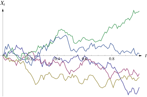
Figure 27: Simulation of the Ornstein-Uhlenbeck process. Five sample paths starting at $\left(0,0\right)$ with mean $\mu=0$, and standard deviation $\sigma=0.3$.

Example 20.8 (Shannon).

$F_{4}\left(x\right)=\left({\displaystyle\frac{\sin\left(x/2\right)}{x/2}}\right)^{2}$; $\left|x\right|<\frac{1}{2}$. $F_{4}$ is concave, and analytic in a neighborhood of $x=0$. By Theorem 21.6, $Ext\left(F_{4}\right)=Ext_{1}\left(F_{4}\right)=$ singleton. Therefore, the spline extension in Figure 28 is not positive definite.

Figure 28: A spline extension of $F_{4}\left(x\right)=\left(\frac{\sin\left(x/2\right)}{x/2}\right)^{2}$; $\Omega=\left(0,\frac{1}{2}\right)$

Example 20.9 (Gaussian distribution).

$F_{5}\left(x\right)=e^{-x^{2}/2}$; $\left|x\right|<1$. $F_{5}$ is concave, analytic in $-1<x<1$. $Ext\left(F_{5}\right)=Ext_{1}\left(F_{5}\right)=$ singleton. The spline extension in Figure 29 is not positive definite (see Theorem 21.6).

Figure 29: A spline extension of $F_{5}\left(x\right)=e^{-x^{2}/2}$; $\Omega=\left(0,1\right)$

Example 20.10.

$F_{6}\left(x\right)=\cos\left(x\right)$; $\left|x\right|<\frac{\pi}{4}$. $F_{6}$ is concave, analytic around $x=0$. By Theorem 21.6, the spline extension in Figure 30 is not positive definite.

Figure 30: A spline extension of $F_{6}\left(x\right)=\cos\left(x\right)$; $\Omega=\left(0,\frac{\pi}{4}\right)$

Lemma 20.11.

The function $\cos x$ is positive definite on $\mathbb{R}$.

Proof 20.12.

For all finite system of coefficients $\left\{c_{j}\right\}$ in $\mathbb{C}$, we have

$$\sum_{j}\sum_{k}\overline{c_{j}}c_{k}\cos\left(x_{j}-x_{k}\right) = \sum_{j}\sum_{k}\overline{c_{j}}c_{k}\left(\cos x_{j}\cos x_{k}+\sin x_{j}\sin x_{k}\right)$$ (260)

$$= \Bigl{|}\sum_{j}c_{j}\cos x_{j}\Bigr{|}^{2}+\Bigl{|}\sum_{j}c_{j}\sin x_{j}\Bigr{|}^{2}\geq 0.$$

∎

Lemma 20.13.

Consider the following two functions $F_{2}\left(x\right)=1-\left|x\right|$, and $F_{3}\left(x\right)=e^{-\left|x\right|}$, each defined on a finite interval $\left(-a,a\right)$, possibly a different value of $a$ from one to the next. The distributional double derivatives are as follows:

$$F_{2}^{\prime\prime} = -2\delta_{0}$$

$$F_{3}^{\prime\prime} = F_{3}-2\delta_{0}$$

where $\delta_{0}$ is Dirac’s delta function (i.e., point mass at $x=0$, $\delta_{0}=\delta\left(x-0\right)$.)

Proof 20.14.

The conclusion follows from a computation, making use of L. Schwartz’ theory of distributions; see Trè (06).     ∎

21 Main Theorems

Now, we shall establish the main result in this chapter (Theorem 21.6) concerning the set $Ext\left(F\right)$. We begin with two preliminary theorems (one is a theorem by Carleman on moments, and the other by Nelson on analytic vectors), and a lemma, which will all be used in our proof of Theorem 21.6.

Theorem 21.1 (Carleman Akh (65)).

Let $\mu$ be a positive Borel measure on $\mathbb{R}$ such that $t^{n}\in L^{1}\left(\mu\right)$ for all $n\in\mathbb{Z}_{+}\cup\left\{0\right\}$, and set $m_{n}:=\int_{\mathbb{R}}t^{n}d\mu\left(t\right)$. If

$$\sum_{k=1}^{\infty}m_{2k}^{-\frac{1}{2k}}=\infty,$$ (261)

then the set of positive measures with these moments is a singleton. We say that the moment problem is determinate.

We recall E. Nelson’s theorem on analytic vectors:

Theorem 21.2 (Nelson Nel (59)).

Let $D$ be a skew-Hermitian operator with dense domain $dom\left(D\right)$ in a Hilbert space. Suppose $dom\left(D\right)$ contains a dense set of vectors $v$ s.t. $\exists\>C_{0},C_{1}<\infty$,

$$\left\|D^{n}v\right\|\leq C_{0}\>n!\>C_{1}^{n},\quad n=0,1,2,\cdots$$ (262)

where the constants $C_{0}$, $C_{1}$ depend on $v$; then $D$ is essentially skew-adjoint, and so it has deficiency indices $\left(0,0\right)$. Vectors satisfying (262) are called analytic vectors.

Lemma 21.3.

Let $F$ be a p.d. function defined on $\left(-a,a\right)$, $a>0$, and assume that $F$ is analytic in a neighborhood of $x=0$; then $D^{\left(F\right)}$ has deficiency indices $\left(0,0\right)$, i.e., $D^{\left(F\right)}$ is essentially skew-adjoint, and so $Ext_{1}\left(F\right)$ is a singleton.

Proof 21.4.

We introduce $\mathscr{H}_{F}$ and $D^{\left(F\right)}$ as before. Recall that $dom(D^{\left(F\right)})$ consists of

$$F_{\varphi}\left(x\right)=\int_{0}^{a}\varphi\left(y\right)F\left(x-y\right)dy,\quad\varphi\in C_{c}^{\infty}\left(0,a\right)$$ (263)

and

$$D^{\left(F\right)}(F_{\varphi})\left(x\right)=F_{\varphi^{\prime}}\left(x\right)=\frac{d}{dx}F_{\varphi}\left(x\right).\;(\mbox{integration by parts})$$ (264)

Since $F$ is locally analytic, we get

$$(D^{\left(F\right)})^{n}F_{\varphi}=\varphi*F^{\left(n\right)},\quad\varphi\in C_{c}^{\infty}\left(0,a\right).$$ (265)

The lemma will be established by the following:

Claim 3.

The vectors $\{F_{\varphi}:\varphi\in C_{c}^{\infty}\left(0,\varepsilon\right)\}$, for sufficiently small $\varepsilon>0$, satisfy the condition in (262). Note that $\left\{F_{\varphi}\right\}$ is dense in $\mathscr{H}_{F}$ by Section 7, so these are analytic vectors in the sense of Nelson (see Theorem 21.2, and Nel (59)).

Proof 21.5.

Since $F$ is assumed to be analytic around $x=0$, there exists $\varepsilon>0$ s.t.

$$F\left(x\right)=\sum_{n=0}^{\infty}\frac{F^{\left(n\right)}\left(y\right)}{n!}\left(x-y\right)^{n}$$ (266)

holds for $\left|x\right|\ll 2\varepsilon$, $\left|y\right|<\varepsilon$; and this implies that

$$\left|F^{\left(n\right)}\left(y\right)\right|\leq C_{0}\>n!\varepsilon^{-n}.$$ (267)

We now use (265) to establish the estimate (262) for $\varepsilon$ as in (266)-(267). We pick $\varepsilon$, and consider $\varphi\in C_{c}^{\infty}\left(0,\varepsilon\right)$, then

$$(D^{\left(F\right)})^{n}F_{\varphi}\left(x\right) = \int_{0}^{\varepsilon}\varphi\left(y\right)F^{\left(n\right)}\left(x-y\right)dy$$ (268)

$$= \int_{0}^{\varepsilon}\varphi\left(x-y\right)F^{\left(n\right)}\left(y\right)dy.$$

Using Corollary 7.12, we get

$$\left\|F^{\left(m\right)}\right\|_{\mathscr{H}_{F}}^{2}=-F^{\left(2m\right)}\left(0\right)$$ (269)

and in particular $F^{\left(2m\right)}\left(0\right)\leq 0$. So,

$$\left\|(D^{\left(F\right)})^{n}\left(F_{\varphi}\right)\right\|_{\mathscr{H}_{F}}^{2} \underset{\text{$\left(\ref{eq:ne8}\right)$}}{\leq} \left(\int_{0}^{\varepsilon}\left|\varphi\right|\right)^{2}\left\|F^{\left(n\right)}\right\|_{\mathscr{H}_{F}}^{2}$$

$$\underset{\text{$\left(\ref{eq:ne9}\right)$}}{\leq} \left(\int_{0}^{\varepsilon}\left|\varphi\right|\right)^{2}\left(-F^{\left(2n\right)}\left(0\right)\right)$$

$$\underset{\text{$\left(\ref{eq:ne7}\right)$}}{\leq} \left(\int_{0}^{\varepsilon}\left|\varphi\right|\right)^{2}C_{0}^{2}\left(\frac{2}{\varepsilon}\right)^{2n}\left(n!\right)^{2};$$

i.e.,

$$\left\|(D^{\left(F\right)})^{n}\left(F_{\varphi}\right)\right\|_{\mathscr{H}_{F}}\leq\left(\int_{0}^{\varepsilon}\left|\varphi\right|\right)C_{0}\left(\frac{2}{\varepsilon}\right)^{n}n!,$$

which is the Nelson estimate (262). This completes the proof of the claim.

Note that in Corollary 7.12, we proved (269) for $m=1$, but it follows in general by induction: $m=1$, $\left\|F^{\prime}\right\|_{\mathscr{H}_{F}}^{2}=-F^{\left(2\right)}\left(0\right)$.

The fact that the set $\{F_{\varphi}:\varphi\in C_{c}^{\infty}\left(0,\varepsilon\right)\}$ is dense in $\mathscr{H}_{F}$ follows from an argument in Nel (59); Jor (87):

Starting with $F_{\varphi}$, $\varphi\in C_{c}^{\infty}\left(0,\varepsilon\right)$, using a local translation, we can move $F_{\varphi}$ towards the endpoint $x=a$. This local translation preserves the $\mathscr{H}_{F}$-norm (see, e.g., the proof of Lemma 8.3), and so $F_{\varphi}\left(\cdot-s\right)$, with sufficiently small $s$, will also satisfy the analytic estimates with the same constants $C$ as that of $F_{\varphi}$. Thus the analytic estimates established for $F_{\varphi}$ with $\varphi\in C_{c}^{\infty}\left(0,\varepsilon\right)$ carries over to the rest of the interval up to the endpoint $x=a$. It remains to note that $\left\{F_{\varphi}:\varphi\in C_{c}^{\infty}\left(0,a\right)\right\}$ is dense in $\mathscr{H}_{F}$; see Lemma 7.4.     ∎

Therefore, we get a dense set of analytic vectors for $D^{\left(F\right)}$ as claimed. By Nelson’s theorem, we conclude that $D^{\left(F\right)}$ is essentially skew-adjoint, so it has deficiency indices $\left(0,0\right)$.     ∎

Theorem 21.6.

Let $F$ be a continuous p.d. function given in some finite interval $\left(-a,a\right)$, $a>0$. Assume that $F$ is analytic in a neighborhood of 0; then $Ext_{2}\left(F\right)$ is empty.

Proof 21.7.

Since $F$ is assumed to be analytic in a neighborhood of $0$, by Lemma 21.3, we see that $D^{\left(F\right)}$ has deficiency indices $\left(0,0\right)$, i.e., it is essentially skew-adjoint; and $Ext_{1}\left(F\right)=\left\{\mu\right\}$, a singleton. Thus,

$$F\left(x\right)=\widehat{d\mu}\left(x\right),\quad\forall x\in\left(-a,a\right).$$ (270)

Also, by the analytic assumption, there exists $c>0$ such that

$$F\left(x\right)=\sum_{n=0}^{\infty}\frac{F^{\left(n\right)}\left(0\right)}{n!}x^{n},\quad\forall\left|x\right|<c;$$ (271)

and using (270), we get that

$$\int_{\mathbb{R}}e^{itx}d\mu\left(t\right)=\sum_{n=0}^{\infty}\frac{\left(ix\right)^{n}}{n!}\int_{\mathbb{R}}t^{n}d\mu\left(t\right),\quad x\in\mathbb{R},\>\left|x\right|<c.$$ (272)

Combining (271) and (272), we see that $\exists 0<c_{1}<c$ such that the $n^{th}$-moment of $\mu$, i.e.,

$$m_{n}=\int_{\mathbb{R}}t^{n}d\mu\left(t\right)=F^{\left(n\right)}\left(0\right)\left(-i\right)^{n}$$ (273)

satisfies the following estimate: $\exists c_{0}<\infty$ such that

$$\left|\frac{x^{n}}{n!}m_{n}\right|\leq c_{0},\quad\forall\left|x\right|\leq c_{1};$$

that is,

$$\left|m_{n}\right|\leq c_{0}\frac{n!}{c_{1}^{n}},\quad\forall n=0,1,2,\cdots.$$ (274)

In particular, all the moments of $\mu$ are finite.

Now, we may apply Carleman’s condition Akh (65) with the estimate in (274), and conclude that there is a unique measure with the moments specified by the r.h.s. of (273); i.e., the measure is uniquely determined by $F$. Therefore, $Ext\left(F\right)=\left\{\mu\right\}$, and so $Ext_{2}\left(F\right)=Ext\left(F\right)\backslash Ext_{1}\left(F\right)=\emptyset$, which is the desired conclusion. (To apply Carleman’s condition, we make use of Stirling’s asymptotic formula for the factorials in (274)).

By Carleman’s theorem (see Theorem 21.1), there is a unique measure with these moments, but by (271) and (273) these moments also determine $F$ uniquely, and vice versa. Hence the conclusion that $Ext(F)$ is a singleton.     ∎

21.1 Some Applications

Below we discuss a family of examples of positive definite functions $F$, defined initially only in the interval $-1<x<1$, but allows analytic continuation to a complex domain,

$$\mathscr{O}^{\mathbb{C}}:=\left\{z\in\mathbb{C}\>|\>\Im\left\{z\right\}>-a\right\},$$

see Figure 32. Here, $a\geq 0$ is fixed.

What is special for this family is that, for each $F$ in the family, the convex set $Ext\left(F\right)$ is a singleton. It has the following form: There is a probability measure $\mu$ on $\mathbb{R}$, such that

$$\widehat{d\mu}\left(\lambda\right)=M\left(\lambda\right)d\lambda,\quad\lambda\in\mathbb{R};$$ (275)

where $M$ is supported on $[0,\infty)$, and $Ext\left(F\right)=\left\{\mu\right\}$, the singleton.

The list of these measures $d\mu=M\left(\lambda\right)d\lambda$ includes the following distributions from statistics:

$$M\left(\lambda\right)=M_{p}\left(\lambda\right)=\frac{\lambda^{p-1}}{\Gamma\left(p\right)}e^{-\lambda},\quad\lambda\geq 0;$$ (276)

where $p$ is fixed, $p>0$, and $\Gamma\left(p\right)$ is the Gamma function. (The case when $p=\frac{1}{2}\mathbb{Z}_{+}$, i.e., $p=\frac{n}{2}$, is called the $\chi_{2}$-distribution of $n$ degrees of freedom. See AMS (13).)

Another example is the log-normal distribution (see KM (04)), where

$$M\left(\lambda\right)=\frac{1}{\sqrt{2\pi}}\frac{1}{\lambda}e^{-\left(\log\lambda-\mu_{0}\right)^{2}/2},$$ (277)

and where $\mu_{0}\in\mathbb{R}$ is fixed. The domain in $\lambda$ is $\lambda>0$. See Figure 31.

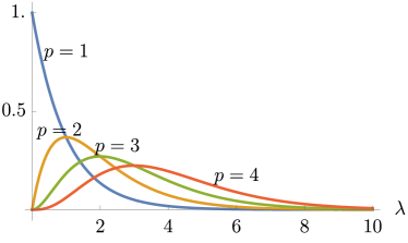
(a) The Gamma (p) distribution with parameter $p$, see (276).

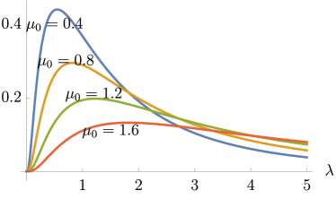
(b) The log-normal distribution with parameter $\mu_{0}$, see (277).

Figure 31: Probability densities of Gamma (p) and log-normal distributions.

Both of the families are given by parameters, but different from one to the other, see (276), Gamma; and 277, log-normal. They have in common the index $(0,0)$ conclusion. More specifically, in each of the two classes, when an initial p.d. function $F$ is specified in a finite interval $(-a,a)$, we compute the associated skew-Hermitian operator $D^{\left(F\right)}$ in $\mathscr{H}_{F}$, and this operator will have deficiency indices $(0,0)$. The big difference between the two classes is that only in the first family will $F$ be analytic in a neighborhood of $x=0$; not for the other. We also stress that these families are very important in applications, see e.g., KT (08); KRAA (15); Lin (14).

We shall consider extension theory for the p.d. functions connected with the first family of these distributions, i.e., (276). The conclusions we list in Example 21.8 below all follow from a direct application of Theorem 21.6.

Example 21.8.

Fix $p\in\mathbb{R}_{+}$, and let $F=F_{p}$ be given by

$$F\left(x\right):=\left(1-ix\right)^{-p},\quad\left|x\right|<1;$$ (278)

i.e., $F$ is defined in the interval $\left(-1,1\right)$. For the study of the corresponding $\mathscr{H}_{F}$, we write $\Omega=\left(0,1\right)$, so that $\Omega-\Omega=\left(-1,1\right)$. The following properties hold:

1. $F$ is positive definite (p.d.) in $\left(-1,1\right)$.

2. $F$ has a unique continuous p.d. extension $\widetilde{F}$ to $\mathbb{R}$.

3. The p.d. extension $\widetilde{F}$ in (2) has an analytic continuation, $x\rightarrow z\in\mathbb{C}$, to the complex domain (Figure 32)

   $$\mathscr{O}^{\mathbb{C}}=\left\{z\in\mathbb{C}\>|\>\Im\left\{z\right\}>-1\right\}.$$ (279)

4. $Ext\left(F\right)$ is a singleton, and $Ext_{2}\left(F\right)=\emptyset$.

5. For the skew-Hermitian operator $D^{\left(F\right)}$ (with dense domain in $\mathscr{H}_{F}$), we get deficiency indices $\left(0,0\right)$.

6. In case of $p=1$, for the corresponding p.d. function $F$ in (278), we have:

   $$\Re F\left(x\right) = \frac{1}{1+x^{2}},\;\mbox{and}$$

   $$\Im F\left(x\right) = \frac{x}{1+x^{2}},\;\mbox{for }\left|x\right|<1.$$

A systematic discussion or the real and the imaginary parts of positive definite functions, and their local properties, is included in Section 33.

Figure 32: The complex domain $\mathscr{O}^{\mathbb{C}}:=\left\{z\in\mathbb{C}\>|\>\Im\left\{z\right\}>-a\right\}$ , $a=1$.

Remark 21.9.

While both the Gamma distribution (276), $p>0$, and the log-normal distribution (277) are supported on the half-line $0\leq\lambda<\infty$, there is an important distinction connected to moments and the Carleman condition (261).

The moments,

$$m_{n}:=\int_{0}^{\infty}\lambda^{n}d\mu\left(\lambda\right)=\int_{0}^{\infty}\lambda^{n}M\left(\lambda\right)d\lambda,$$

for the two cases are as follows:

1. Gamma (p):

   $$m_{n}=\left(p+n-1\right)\left(p+n-2\right)\cdots\left(p+1\right)p,\quad n\in\mathbb{Z}_{+}$$ (280)

2. log-normal ($\mu_{0}$):

   $$m_{n}=e^{\mu_{0}n+n^{2}/2},\quad n\in\mathbb{Z}_{+}.$$ (281)

Since both are Stieltjes-problems, the Carleman condition is

$$\sum_{n=1}^{\infty}m_{n}^{-\frac{1}{2n}}=\infty.$$ (282)

One checks that (282) is satisfied for Gamma (p), see (280); but not for log-normal ($\mu_{0}$) case, see (281). A closer inspection shows that the generating function,

$$F_{LN}\left(x\right)=\widehat{d\mu_{LN}}\left(x\right),\quad x\in\mathbb{R},$$ (283)

for log-normal ($\mu_{0}$) is not analytic in a neighborhood of $x=0$, see (277). In fact, we have

$$F_{LN}\left(x\right)=\frac{1}{\sqrt{2\pi}}\int_{-\infty}^{\infty}\exp\left[-\frac{\lambda^{2}}{2}+ixe^{\lambda}\right]d\lambda$$ (284)

which has a complex analytic continuation: $x\mapsto z$, $\Im\left\{z\right\}>0$, the open upper half-plane (UH); but fails to be analytic on $x$-axis, the boundary of $UH$.

Note the formal power series,

$$F_{LN}\left(x\right)\>\mbox{"="}\>\sum_{n=0}^{\infty}e^{n^{2}/2}\frac{\left(ix\right)^{n}}{n!},$$ (285)

is divergent.More precisely, the radius of convergence in the “power series” on the r.h.s. (285) is $rad=0$. And, as a result $F_{LN}\left(x\right)$ is not analytic in a neighborhood of $x=0$.

22 The Deficiency-Indices of $D^{\left(F\right)}$

This section is devoted to the index problem for the skew-Hermitian operator $D^{\left(F\right)}$ (with dense domain in the RKHS $\mathscr{H}_{F}$), but not in the general case. Rather we compute $D^{\left(F\right)}$ for the particular choice of partially defined p.d. functions $F$ from the list in Table 1. There are six of them in all, numbered $F_{1}$ through $F_{6}$. The last one $F_{6}$ is the easiest, and we begin with it. While these are only special cases (for example, they are all continuous p.d. functions defined initially only in a fixed finite interval, centered at $x=0$), a closer analysis of them throws light on much more general cases, including domains in $\mathbb{R}^{n}$, and even in non-abelian groups. But even for the case of $G=\mathbb{R}$, we stress that applications to statistics dictates a study of extension theory for much bigger families of interesting p.d. functions, defined on finite intervals; see for example Section 21.1.

$F:\left(-a,a\right)\rightarrow\mathbb{C}$	Indices	The Operator $D^{\left(F\right)}$
$F_{1}\left(x\right)=\frac{1}{1+x^{2}}$, $\left|x\right|<1$	$\left(0,0\right)$	$D^{\left(F\right)}$ unbounded, skew-adjoint
$F_{2}\left(x\right)=1-\left|x\right|$, $\left|x\right|<\frac{1}{2}$	$\left(1,1\right)$	$D^{\left(F\right)}$ has unbounded skew-adjoint extensions
$F_{3}\left(x\right)=e^{-\left|x\right|}$, $\left|x\right|<1$	$\left(1,1\right)$	$D^{\left(F\right)}$ has unbounded skew-adjoint extensions
$F_{4}\left(x\right)=\left(\frac{\sin\left(x/2\right)}{x/2}\right)^{2}$, $\left|x\right|<\frac{1}{2}$	$\left(0,0\right)$	$D^{\left(F\right)}$ bounded, skew-adjoint
$F_{5}\left(x\right)=e^{-x^{2}/2}$, $\left|x\right|<1$	$\left(0,0\right)$	$D^{\left(F\right)}$ unbounded, skew-adjoint
$F_{6}\left(x\right)=\cos x$, $\left|x\right|<\frac{\pi}{4}$	$\left(0,0\right)$	$D^{\left(F\right)}$ is rank-one, $\dim\left(\mathscr{H}_{F_{6}}\right)=2$
$F_{7}\left(x\right)=\left(1-ix\right)^{-p}$, $\left|x\right|<1$	$\left(0,0\right)$	$D^{\left(F\right)}$ is unbounded, skew-adjoint, but semibounded; see Corollary (8.29)

Table 1: The deficiency indices of $D^{\left(F\right)}:F_{\varphi}\mapsto F_{\varphi^{\prime}}$, with $F=F_{i}$, $i=1,\cdots,7$.

We have introduced a special class of positive definite (p.d.) extensions using a spline technique based on a theorem by Pólya Pól (49).

We then get a deficiency index-problem (see e.g., vN32a ; Kre (46); DS (88); AG (93); Nel (69)) in the RKHSs $\mathscr{H}_{F_{i}}$, $i=1,\ldots,6$, for the operator $D^{\left(F_{i}\right)}F_{\varphi}^{\left(i\right)}=F_{\varphi^{\prime}}^{\left(i\right)}$, $\forall\varphi\in C_{c}^{\infty}\left(0,a\right)$. As shown in Tables 1, $D^{\left(F_{2}\right)}$ and $D^{\left(F_{3}\right)}$ have indices $\left(1,1\right)$, and the other four all have indices $\left(0,0\right)$.

Following is an example with deficiency indices $\left(0,0\right)$

Lemma 22.1.

$\mathscr{H}_{F_{6}}$ is 2-dimensional.

Proof 22.2.

For all $\varphi\in C_{c}^{\infty}\left(0,\frac{\pi}{4}\right)$, we have:

$$\int_{\Omega}\int_{\Omega}\overline{\varphi\left(x\right)}\varphi\left(y\right)F_{6}\left(x-y\right)dxdy$$

$$= \left|\int_{\Omega}\varphi\left(x\right)\cos xdx\right|^{2}+\left|\int_{\Omega}\varphi\left(x\right)\sin xdx\right|^{2}$$

$$= \left|\widehat{\varphi}^{\left(c\right)}\left(1\right)\right|^{2}+\left|\widehat{\varphi}^{\left(s\right)}\left(1\right)\right|^{2}$$ (286)

where $\widehat{\varphi}^{\left(c\right)}=$ the cosine-transform, and $\widehat{\varphi}^{\left(s\right)}=$ the sine-transform.     ∎

So the deficiency indices only account from some of the extension of a given positive definite function $F$ on $\Omega-\Omega$, the Type I extensions.

Except for $\mathscr{H}_{F_{6}}$ (2-dimensional), in all the other six examples, $\mathscr{H}_{F_{i}}$ is infinite-dimensional.

In the given seven examples, we have p.d. extensions to $\mathbb{R}$ of the following form, $\widehat{d\mu_{i}}\left(\cdot\right)$, $i=1,\ldots,7$, where these measures are as follows:

$d\mu_{1}\left(\lambda\right)=\frac{1}{2}e^{-\left|\lambda\right|}d\lambda$	Fig 41 (pg. 41)
$d\mu_{2}\left(\lambda\right)=\frac{1}{2\pi}\left(\frac{\sin\left(\lambda/2\right)}{\lambda/2}\right)^{2}d\lambda$	Fig 41 (pg. 41); Table 6 (pg. 6)
$d\mu_{3}\left(\lambda\right)=\frac{d\lambda}{\pi\left(1+\lambda^{2}\right)}$	Fig 41 (pg. 41); Table 6 (pg. 6)
$d\mu_{4}\left(\lambda\right)=\chi_{\left(-1,1\right)}\left(\lambda\right)\left(1-\left|\lambda\right|\right)d\lambda$	Fig 41 (pg. 41); Ex 29.17 (pg. 29.17); Ex 20.8 (pg. 20.8)
$d\mu_{5}\left(\lambda\right)=\frac{1}{\sqrt{2\pi}}e^{-\lambda^{2}/2}d\lambda$	Fig 41 (pg. 41); Ex 3.1 (pg. 3.1)
$d\mu_{6}\left(\lambda\right)=\frac{1}{2}\left(\delta_{1}+\delta_{-1}\right)$	Fig 41 (pg. 41); Lemma 20.11 (pg. 20.11); Thm 28.4 (pg. 28.4); Thm 28.16 (pg. 28.16); Rem 29.8 (pg. 29.8)
$d\mu_{7}\left(\lambda\right)=\frac{\lambda^{p}}{\Gamma\left(p\right)}e^{-\lambda}d\lambda$, $\lambda\geq 0$	Fig 41 (pg. 41); Fig 31a (pg. 31a)

Table 2: The canonical isometric embeddings: $\mathscr{H}_{F_{i}}\hookrightarrow L^{2}\left(\mathbb{R},d\mu_{i}\right)$, $i=1,\ldots,7$. In each case, we have $\mu_{i}\in Ext\left(F_{i}\right)$, and, by Corollary 12.15 therefore, the corresponding isometric embeddings $T_{\mu_{i}}$ mapping into the respective $L^{2}\left(\mu_{i}\right)$-Hilbert spaces.

See also Table 7 and Figure 41 below.

Corollary 22.3.

For $i=1,\cdots,6$, we get isometries $T^{\left(i\right)}:\mathscr{H}_{F_{i}}\rightarrow L^{2}\left(\mathbb{R},\mu_{i}\right)$, determined by

$$T^{\left(i\right)}(F_{\varphi}^{\left(i\right)})=\widehat{\varphi},\quad\forall\varphi\in C_{c}^{\infty}\left(\Omega_{i}\right);\;\mbox{where}$$

$$\|F_{\varphi}^{\left(i\right)}\|_{\mathscr{H}_{F_{i}}}^{2}=\left\|\widehat{\varphi}\right\|_{L^{2}\left(\mu_{i}\right)}^{2}=\int_{\mathbb{R}}\left|\widehat{\varphi}\right|^{2}d\mu_{i}.$$

Note that, except for $i=6$, $T^{\left(i\right)}$ is only isometric into $L^{2}\left(\mu_{i}\right)$.

The adjoint operator, $(T^{\left(i\right)})^{*}:L^{2}\left(\mathbb{R},\mu_{i}\right)\rightarrow\mathscr{H}_{F_{i}}$, is given by

$$(T^{\left(i\right)})^{*}f=\chi_{\overline{\Omega_{i}}}\left(fd\mu_{i}\right)^{\vee},\quad\forall f\in L^{2}\left(\mathbb{R},\mu_{i}\right).$$

Proof 22.4.

We refer to Corollary 12.15.     ∎

Example 22.5 (An infinite-dimensional example as a version of $F_{6}$).

Fix $p$, $0<p<1$, and set

$$F_{p}\left(x\right):=\prod_{n=1}^{\infty}\cos\left(2\pi p^{n}x\right).$$

Then $F_{p}=\widehat{d\mu_{p}}$, where $\mu_{p}$ is the Bernoulli measure, and so $F_{p}$ is a continuous positive definite function on $\mathbb{R}$. Note that some of those measures $\mu_{p}$ are fractal measures.

For fixed $p\in\left(0,1\right)$, the measure $\mu_{p}$ is the law (i.e., distribution) of the following random power series

$$X_{p}\left(\omega\right):=\sum_{n=1}^{\infty}\left(\pm\right)p^{n},$$

where $\omega\in\prod{}_{1}^{\infty}\left\{\pm 1\right\}$ (= infinite Cartesian product) and where the distribution of each factor is $\left\{-\frac{1}{2},\frac{1}{2}\right\}$, and statically independent. For relevant references on random power series, see Neu (13); Lit (99).

Pólya-extensions

The extensions we generate with the application of Pólya’s theorem are realized in a bigger Hilbert space. The deficiency indices of the skew-Hermitian operator $D^{\left(F\right)}$ are computed w.r.t. the RKHS $\mathscr{H}_{F}$, i.e., for the “small” p.d. function $F:\Omega-\Omega\rightarrow\mathbb{C}$.

Example 22.6.

$F_{2}\left(x\right)=1-\left|x\right|$, $\left|x\right|<\frac{1}{2}$, has the obvious p.d. extension to $\mathbb{R}$, i.e., $\left(1-\left|x\right|\right)\chi_{\left[-1,1\right]}\left(x\right)$, which corresponds to the measure $\mu_{2}$ from Table 2. It also has other p.d. extensions, e.g., the Pólya extension in Figure 25. All these extensions are of Type II, realized in $\infty$-dimensional dilation-Hilbert spaces.

We must make a distinction between two classes of p.d. extensions of $F:\Omega-\Omega\rightarrow\mathbb{C}$ to continuous p.d. functions on $\mathbb{R}$.

Case 1. There exists a unitary representation $U\left(t\right):\mathscr{H}_{F}\rightarrow\mathscr{H}_{F}$ such that

$$F\left(t\right)=\left\langle\xi_{0},U\left(t\right)\xi_{0}\right\rangle_{\mathscr{H}_{F}},\>t\in\Omega-\Omega$$ (287)

Case 2. (e.g., Pólya extension) There exist a dilation-Hilbert space $\mathscr{K}$, and an isometry $J:\mathscr{H}_{F}\rightarrow\mathscr{K}$, and a unitary representation $U\left(t\right)$ of $\mathbb{R}$ acting in $\mathscr{K}$, such that

$$F\left(t\right)=\left\langle J\xi_{0},U\left(t\right)J\xi_{0}\right\rangle_{\mathscr{K}},\>t\in\Omega-\Omega$$ (288)

In both cases, $\xi_{0}=F\left(0-\cdot\right)\in\mathscr{H}_{F}$.

In case 1, the unitary representation is realized in $\mathscr{H}_{\left(F,\Omega-\Omega\right)}$, while, in case 2, the unitary representation $U\left(t\right)$ lives in the expanded Hilbert space $\mathscr{K}$.

Note that the r.h.s. in both (287) and (288) is defined for all $t\in\mathbb{R}$.

Lemma 22.7.

Let $F_{ex}$ be one of the Pólya extensions if any. Then by the Galfand-Naimark-Segal (GNS) construction applied to $F_{ext}:\mathbb{R}\rightarrow\mathbb{R}$, there is a Hilbert space $\mathscr{K}$ and a vector $v_{0}\in\mathscr{K}$ and a unitary representation $\left\{U\left(t\right)\right\}_{t\in\mathbb{R}};$ $U\left(t\right):\mathscr{K}\rightarrow\mathscr{K}$, such that

$$F_{ex}\left(t\right)=\left\langle v_{0},U\left(t\right)v_{0}\right\rangle_{\mathscr{K}},\>\forall t\in\mathbb{R}.$$ (289)

Setting $J:\mathscr{H}_{F}\rightarrow\mathscr{K}$, $J\xi_{0}=v_{0}$, then $J$ defines (by extension) an isometry such that

$$U\left(t\right)J\xi_{0}=J\left(\mbox{local translation in }\Omega\right)$$ (290)

holds locally (i.e., for $t$ sufficiently close to $0$.)

Moreover, the function

$$\mathbb{R}\ni t\mapsto U\left(t\right)J\xi_{0}=U\left(t\right)v_{0}$$ (291)

is compactly supported.

Proof 22.8.

The existence of $\mathscr{K}$, $v_{0}$, and $\left\{U\left(t\right)\right\}_{t\in\mathbb{R}}$ follows from the GNS-construction.

The conclusions in (290) and (291) follow from the given data, i.e., $F:\Omega-\Omega\rightarrow\mathbb{R}$, and the fact that $F_{ex}$ is a spline-extension, i.e., it is of compact support; but by (289), this means that (291) is also compactly supported.     ∎

Example 20.5 gives a p.d. $F$ in $\left(-\tfrac{1}{2},\tfrac{1}{2}\right)$ with $D^{(F)}$ of index $(1,1)$ and explicit measures in $Ext_{1}(F)$ and in $Ext_{2}(F).$

We have the following:

Deficiency $\left(0,0\right)$: The p.d. extension of Type I is unique; see (287); but there may still be p.d. extensions of Type II; see (288).

Deficiency $\left(1,1\right)$: This is a one-parameter family of extensions of Type I; and some more p.d. extensions are Type II.

So we now divide

$$Ext\left(F\right)=\left\{\mu\in\mbox{Prob}\left(\mathbb{R}\right)\>\big{|}\>\widehat{d\mu}\mbox{ is an extension of }F\right\}$$

up in subsets

$$Ext\left(F\right)=Ext_{type1}\left(F\right)\cup Ext_{type2}\left(F\right);$$

where $Ext_{2}\left(F\right)$ corresponds to the Pólya extensions.

Table 3: Type II extensions. Six cases of p.d. continuous functions defined on a finite interval. Additional properties of these functions will be outlined in Section 34. For each of the six graphs (of p.d. function), the numbers $(0,0)$ or $(1,1)$ indicate the deficiency indices. The case $(0,0)$ means “unique skew-adjoint extension”; while $(1,1)$ means that there is a one-parameter family of distinct skew-adjoint extensions. For each of the cases of the locally defined p.d. functions $F_{1}$, $F_{4}$, $F_{5}$, and $F_{6}$, we know that sets $Ext(F)$ are singletons. This follows from Theorem 21.6.

Return to a continuous p.d. function $F:\left(-a,a\right)\rightarrow\mathbb{C}$, we take for the RKHS $\mathscr{H}_{F}$, and the skew-Hermitian operator

$$D\left(F_{\varphi}\right)=F_{\varphi^{\prime}},\>\varphi^{\prime}=\frac{d\varphi}{dx}$$

If $D\subseteq A$, $A^{*}=-A$ in $\mathscr{H}_{F}$ then there exists an isometry $J:\mathscr{H}_{F}\rightarrow L^{2}\left(\mathbb{R},\mu\right)$, where $d\mu\left(\cdot\right)=\left\|P_{U}\left(\cdot\right)\xi_{0}\right\|^{2}$,

$$U_{A}\left(t\right)=e^{tA}=\int_{\mathbb{R}}e^{it\lambda}P_{U}\left(d\lambda\right),$$

$\xi_{0}=F\left(\cdot-0\right)\in\mathscr{H}_{F}$, $J\xi_{0}=1\in L^{2}\left(\mu\right)$.

23 The Example 20.6, Green’s function, and an $\mathscr{H}_{F}$-ONB

Here, we study Example 20.6 in more depth, and we compute the spectral date of the corresponding Mercer operator. Recall that

$$F\left(x\right):=\begin{cases}e^{-\left|x\right|}&\left|x\right|<1\\ e^{-1}\left(2-\left|x\right|\right)&1\leq\left|x\right|<2\\ 0&\left|x\right|\geq 2\end{cases}$$ (292)

See 33 below.

Figure 33: A Pólya (spline) extension of $F_{3}\left(x\right)=e^{-\left|x\right|}$; $\Omega=\left(-1,1\right)$.

Proposition 23.1.

The RKHS $\mathscr{H}_{F}$ for the spline extension $F$ in (292) has the following ONB:

$$\left\{\left(\frac{2}{1+\left(\frac{\pi n}{2}\right)^{2}}\right)^{\frac{1}{2}}\sin\left(\frac{n\pi x}{2}\right)\right\}_{n\in\mathbb{Z}_{+}.}$$

Proof 23.2.

The distributional derivative of $F$ satisfies

$$F^{\prime\prime} = F-2\delta_{0}+e^{-1}\left(\delta_{2}+\delta_{-2}\right)$$

$$\Updownarrow$$

$$\left(1-\triangle\right)F = 2\delta_{0}-e^{-1}\left(\delta_{2}+\delta_{-2}\right)$$

This can be verified directly, using Schwartz’ theory of distributions. See 20.13 and Trè (06).

Thus, for

$$F_{x}\left(\cdot\right):=F\left(x-\cdot\right)$$

we have the translation

$$\left(1-\triangle\right)F_{x}=2\delta_{x}-e^{-1}\left(\delta_{x-2}+\delta_{x+2}\right)$$ (293)

Consider the Mercer operator (see Section 24):

$$L^{2}\left(0,2\right)\ni g\longmapsto\int_{0}^{2}F_{x}\left(y\right)g\left(y\right)dy=\left\langle F_{x},g\right\rangle.$$

Suppose $\lambda\in\mathbb{R}$, and

$$\left\langle F_{x},g\right\rangle=\lambda g\left(x\right).$$ (294)

Applying $\left(1-\triangle\right)$ to both sides of (294), we get

$$\left\langle\left(1-\triangle\right)F_{x},g\right\rangle=\lambda\left(g\left(x\right)-g^{\prime\prime}\left(x\right)\right),\;0<x<2.$$ (295)

By (293), we also have

$$\left\langle\left(1-\triangle\right)F_{x},g\right\rangle=2g\left(x\right),\;0<x<2;$$ (296)

using the fact the two Dirac masses in (293), i.e., $\delta_{x\pm 2}$, are supported outside the open interval $\left(0,2\right)$.

Therefore, combining (295)-(296), we have

$$g^{\prime\prime}=\frac{\lambda-2}{\lambda}g,\;\forall x\in\left(0,2\right).$$

By Mercer’s theorem, $0<\lambda<2$. Setting

$$k:=\sqrt{\frac{2-\lambda}{\lambda}}\;\left(\Leftrightarrow\lambda=\frac{2}{1+k^{2}}\right)$$

we have

$$g^{\prime\prime}=-k^{2}g,\;\forall x\in\left(0,2\right).$$

Boundary conditions:

In (295), set $x=0$, and $x=2$, we get

$$2g\left(0\right)-e^{-1}g\left(2\right) = \lambda\left(g\left(0\right)-g^{\prime\prime}\left(0\right)\right)$$ (297)

$$2g\left(2\right)-e^{-1}g\left(0\right) = \lambda\left(g\left(2\right)-g^{\prime\prime}\left(2\right)\right)$$ (298)

Now, assume

$$g\left(x\right)=Ae^{ikx}+Be^{-ikx};$$

where

$$g\left(0\right) = A+B$$

$$g\left(2\right) = Ae^{ik2}+Be^{-ik2}$$

$$g^{\prime\prime}\left(0\right) = -k^{2}\left(A+B\right)$$

$$g^{\prime\prime}\left(2\right) = -k^{2}\left(Ae^{ik2}+Be^{-ik2}\right).$$

Therefore, for (297), we have

$$2\left(A+B\right)-e^{-1}\left(Ae^{ik2}+Be^{-ik2}\right) = \lambda\left(1+k^{2}\right)\left(A+B\right)$$

$$= 2\left(A+B\right)$$

i.e.,

$$Ae^{ik2}+Be^{-ik2}=0.$$ (299)

Now, from (298) and using (299), we have

$$A=-B.$$ (300)

Combining (299)-(300), we conclude that

$$\sin 2k=0\Longleftrightarrow k=\frac{\pi n}{2},\;n\in\mathbb{Z};$$

i.e.,

$$\lambda_{n}:=\frac{2}{1+\left(\dfrac{n\pi}{2}\right)^{2}},\;n\in\mathbb{N}.$$ (301)

The associated ONB in $L^{2}\left(0,2\right)$ is

$$\xi_{n}\left(x\right)=\sin\left(\frac{n\pi x}{2}\right),\;n\in\mathbb{N}.$$ (302)

And the corresponding ONB in $\mathscr{H}_{F}$ consists of the functions $\left\{\sqrt{\lambda_{n}}\xi_{n}\right\}_{n\in\mathbb{N}}$, i.e.,

$$\left\{\frac{\sqrt{2}}{\bigl{(}1+\bigl{(}\frac{n\pi}{2}\bigr{)}^{2}\bigr{)}^{1/2}}\sin\left(\frac{n\pi x}{2}\right)\right\}_{n\in\mathbb{N}}$$ (303)

which is the desired conclusion.     ∎

Chapter 6 Spectral Theory for Mercer Operators, and Implications for $Ext\left(F\right)$

Given a continuous positive definite (p.d.) function $F$ on the open interval $\left(-1,1\right)$, we are concerned with the set $Ext\left(F\right)$ of its extensions to p.d. functions defined on all of $\mathbb{R}$, as well as a certain subset $Ext_{1}\left(F\right)$ of $Ext\left(F\right)$. Since every such p.d. extension of $F$ is a Bochner transform of a unique positive and finite Borel measure $\mu$ on $\mathbb{R}$, i.e., $\widehat{d\mu}\left(x\right)$, $x\in\mathbb{R}$ and $\mu\in\mathscr{M}_{+}\left(\mathbb{R}\right)$, we will speak of $Ext\left(F\right)$ as a subset of $\mathscr{M}_{+}\left(\mathbb{R}\right)$. The purpose of this chapter is to gain insight into the nature and properties of $Ext_{1}\left(F\right)$.

In Section 24, we study the Mercer operator $T_{F}$ associated with $F$, which is a certain trace class integral operator. We use it (see Section 25) to identify a natural Bessel frame in the RKHS $\mathscr{H}_{F}$. We further introduce a notion of Shannon sampling of finite Borel measures on $\mathbb{R}$, then use this in Corollary 25.5 to give a necessary and sufficient condition: $\mu\in\mathscr{M}_{+}\left(\mathbb{R}\right)$ is in $Ext\left(F\right)$ if and only if the Shannon sampling of $\mu$ recovers the p.d. function $F$ on the interval $\left(-1,1\right)$.

Definition 23.3.

Let $F$ be a continuous positive definite (p.d.) function on a finite interval $\left(-a,a\right)\subset\mathbb{R}$. By a Mercer operator, we mean the integral operator $T_{F}:L^{2}\left(0,a\right)\rightarrow L^{2}\left(0,a\right)$, given by

$$\left(T_{F}\varphi\right)\left(x\right):=\int_{0}^{a}\varphi\left(y\right)F\left(x-y\right)dy,\quad\varphi\in L^{2}\left(0,a\right),\>x\in\left(0,a\right).$$ (304)

Lemma 23.4.

Let $T_{F}$ be the Mercer operator in (304), and $\mathscr{H}_{F}$ be the RKHS of $F$.

1. Then there is a sequence $\left(\lambda_{n}\right)_{n\in\mathbb{N}}$, $\lambda_{n}>0$, $\sum_{n\in\mathbb{N}}\lambda_{n}<\infty$; and a system of orthogonal functions $\left\{\xi_{n}\right\}\subset L^{2}\left(0,a\right)\cap\mathscr{H}_{F}$, such that

   $$F\left(x-y\right)=\sum_{n\in\mathbb{N}}\lambda_{n}\xi_{n}\left(x\right)\overline{\xi_{n}\left(y\right)},\mbox{ and}$$ (305)

   $$\int_{0}^{a}\overline{\xi_{n}\left(x\right)}\xi_{m}\left(x\right)dx=\delta_{n,m},\quad n,m\in\mathbb{N}.$$ (306)

2. In particular, $T_{F}$ is trace class in $L^{2}\left(0,a\right)$. If $F\left(0\right)=1$, then

   $$trace\left(T_{F}\right)=a.$$ (307)

Proof 23.5.

This is an application of Mercer’s theorem LP (89); FR (42); FM (13). Note that we must check that $F$, initially defined on $\left(-a,a\right)$, extends uniquely by limit to a continuous p.d. function on the closed interval $\left[-a,a\right]$. This is easy to verify; also see Lemma 29.5.     ∎

Corollary 23.6.

Let $F:\left(-a,a\right)\rightarrow\mathbb{C}$ be a continuous p.d. function, assume that $F\left(0\right)=1$. Let $D^{\left(F\right)}$ be the skew-Hermitian operator in $\mathscr{H}_{F}$. Let $z\in\mathbb{C}\backslash\left\{0\right\}$, and $DEF_{F}\left(z\right)\subset\mathscr{H}_{F}$ be the corresponding deficiency space.

Let $\left\{\xi_{n}\right\}_{n\in\mathbb{N}}\subset\mathscr{H}_{F}\cap L^{2}\left(\Omega\right)$, $\Omega:=\left(0,a\right)$; and $\left\{\lambda_{n}\right\}_{n\in\mathbb{N}}$ s.t. $\lambda_{n}>0$, and $\sum_{n=1}^{\infty}\lambda_{n}=a$, be one Mercer–system as in Lemma 23.4.

Then $DEF_{F}\left(z\right)\neq 0$ if and only if

$$\sum_{n=1}^{\infty}\frac{1}{\lambda_{n}}\left|\int_{0}^{a}\overline{\xi_{n}\left(x\right)}e^{zx}dx\right|^{2}<\infty.$$ (308)

Proof 23.7.

We saw in Lemma 23.4 that if $\left\{\xi_{n}\right\}_{n\in\mathbb{N}}$, $\left\{\lambda_{n}\right\}_{n\in\mathbb{N}}$, is a Mercer system (i.e., the spectral data for the Mercer operator $T_{F}$ in $L^{2}\left(0,a\right)$), then $\xi_{n}\in\mathscr{H}_{F}\cap L^{2}\left(\Omega\right)$; and $\left(\sqrt{\lambda_{n}}\xi_{n}\left(\cdot\right)\right)_{n\in\mathbb{N}}$ is an ONB in $\mathscr{H}_{F}$.

But (308) in the corollary is merely stating that the function $e_{z}\left(x\right):=e^{zx}$ has a finite $l^{2}$-expansion relative to this ONB. The rest is an immediate application of Parseval’s identity (w.r.t. this ONB.)     ∎

Remark 23.8.

The conclusion in the corollary applies more generally: It shows that a continuous function $f$ on $\left[0,a\right]$ is in $\mathscr{H}_{F}$ iff

$$\sum_{n=1}^{\infty}\frac{1}{\lambda_{n}}\left|\int_{0}^{a}\overline{\xi_{n}\left(x\right)}f\left(x\right)dx\right|^{2}<\infty.$$

24 Groups, Boundary Representations, and Renormalization

In this section, we study a boundary representation for the operator $T_{F}$ (Corollary 24.13), and an associated renormalization for the Hilbert space $\mathscr{H}_{F}$ in Corollary 24.15, in Theorems 24.9 and 25.8, with corollaries.

Definition 24.1.

Let $G$ be a Lie group, and let $\Omega$ be a subset of $G$, satisfying the following:

1. $\Omega\neq\emptyset$;

2. $\Omega$ is open and connected;

3. the closure $\overline{\Omega}$ is compact;

4. the boundary of $\overline{\Omega}$ has Haar measure zero.

Then, for any continuous positive definition function $F:\Omega^{-1}\cdot\Omega\rightarrow\mathbb{C}$, a trace class Mercer operator is defined by

$$\left(T_{F}\varphi\right)\left(x\right)=\int_{\Omega}\varphi\left(y\right)F\left(y^{-1}x\right)dy,\quad\varphi\in L^{2}\left(\Omega\right)$$ (309)

where $dy$ is the restriction of Haar measure on $G$ to $\Omega$, or equivalently to $\overline{\Omega}$.

Note that with Lemma 29.5 and assumption B3, we conclude that

$$\mathscr{H}_{F}\subseteq C\left(\overline{\Omega}\right)\subset L^{2}\left(\Omega\right).$$ (310)

It is natural to ask: “What is the orthogonal complement of $\mathscr{H}_{F}$ in the larger Hilbert space $L^{2}\left(\Omega\right)$?” The answer is given in Corollary 24.4. We will need the following:

Lemma 24.2.

There is a finite constant $C_{1}$ such that

$$\left\|\xi\right\|_{L^{2}\left(\Omega\right)}\leq C_{1}\left\|\xi\right\|_{\mathscr{H}_{F}},\quad\forall\xi\in\mathscr{H}_{F}.$$ (311)

Proof 24.3.

Since $\mathscr{H}_{F}\subset L^{2}\left(\Omega\right)$ by (310), the inclusion mapping, $\mathscr{H}_{F}\rightarrow L^{2}\left(\Omega\right)$, is closed and therefore bounded; by the Closed-Graph Theorem DS (88); and so the estimate (311) follows. (See also Theorem 24.17 below for an explicit bound $C_{1}$.)     ∎

Corollary 24.4.

Let $T_{F}$ be the Mercer operator in (309), then

$$L^{2}\left(\Omega\right)\ominus\mathscr{H}_{F}=ker\left(T_{F}\right);$$ (312)

and as an operator in $L^{2}\left(\Omega\right)$, $T_{F}$ takes the form:

$$T_{F}=\quad\blockarray{ccc}\scriptstyle{\mathscr{H}_{F}}&\scriptstyle{ker(T_{F})}\\ \block{(cc)c}T_{F}0\quad\scriptstyle{\mathscr{H}_{F}}\\ 00\quad\scriptstyle{ker(T_{F})}\\$$

Proof 24.5.

Let $\xi\in\mathscr{H}_{F}$, and pick $\varphi_{n}\in C_{c}\left(\Omega\right)$ such that

$$\left\|\xi-F_{\varphi_{n}}\right\|_{\mathscr{H}_{F}}\rightarrow 0,\quad n\rightarrow\infty.$$ (313)

Since $F_{\varphi_{n}}=T_{F}\varphi_{n}$, and so we get

$$\left\|\xi-T_{F}\varphi_{n}\right\|_{L^{2}\left(\Omega\right)}\underset{\left(\ref{eq:m-3-3}\right)}{\leq}C_{1}\left\|\xi-F_{\varphi_{n}}\right\|_{\mathscr{H}_{F}}\underset{\left(\ref{eq:m-3-4}\right)}{\longrightarrow}0,\quad n\rightarrow\infty.$$ (314)

Therefore, if $f\in L^{2}\left(\Omega\right)$ is given, we conclude that the following properties are equivalent:

$$\left\langle f,\xi\right\rangle_{L^{2}\left(\Omega\right)} = 0,\;\forall\xi\in\mathscr{H}_{F}$$

$$\Updownarrow$$ by (314)

$$\left\langle f,F_{\varphi}\right\rangle_{L^{2}\left(\Omega\right)} = 0,\;\forall\varphi\in C_{c}\left(\Omega\right)$$

$$\Updownarrow$$

$$\left\langle f,T_{F}\varphi\right\rangle_{L^{2}\left(\Omega\right)} = 0,\;\forall\varphi\in C_{c}\left(\Omega\right)$$

$$\Updownarrow T_{F} L^{2}\left(\Omega\right)$$ ( is selfadjoint, as an operator in .)

$$\left\langle T_{F}f,\varphi\right\rangle_{L^{2}\left(\Omega\right)} = 0,\;\forall\varphi\in C_{c}\left(\Omega\right)$$

$$\Updownarrow C_{c} \left(\Omega\right) L^{2}\left(\Omega\right)$$ ( is dense in )

$$T_{F}f = 0$$

∎

Remark 24.6.

Note that $ker\left(T_{F}\right)$ may be infinite dimensional. This happens for example, in the cases studied in Section 16, and in the case of $F_{6}$ in Table 1. On the other hand, these examples are rather degenerate since the corresponding RKHSs $\mathscr{H}_{F}$ are finite dimensional.

Convention. When computing $T_{F}\left(f\right)$, $f\in L^{2}\left(\Omega\right)$, we may use (310) to write $f=f^{\left(F\right)}+f^{\left(K\right)}$, where $f^{\left(F\right)}\in\mathscr{H}_{F}$, $f^{\left(K\right)}\in ker\left(T_{F}\right)$, and $\langle f^{\left(F\right)},f^{\left(K\right)}\rangle_{L^{2}\left(\Omega\right)}=0$. As a result,

$$T_{F}\left(f\right)=T_{F}f^{\left(F\right)}+T_{F}f^{\left(K\right)}=T_{F}f^{\left(F\right)}.$$

For the inverse operator, by $T_{F}^{-1}\left(f\right)$ we mean $T_{F}^{-1}f^{\left(F\right)}$.

Corollary 24.7.

Let $G$, $\Omega$, $F$ and $\mathscr{H}_{F}$ be as above, assume that $\Omega\subset G$ satisfies B1-B4. Suppose in addition that $G=\mathbb{R}^{n}$, and that there exists $\mu\in Ext\left(F\right)$ such that the support of $\mu$, $suppt\left(\mu\right)$, contains a non-empty open subset in $\mathbb{R}^{n}$; then $ker\left(T_{F}\right)=0$.

Proof 24.8.

By Corollary 12.15, there is an isometry $\mathscr{H}_{F}\rightarrow L^{2}\left(\mathbb{R}^{n},\mu\right)$, by $F_{\varphi}\mapsto\widehat{\varphi}$, for all $\varphi\in C_{c}\left(\Omega\right)$, and so $\left\|F_{\varphi}\right\|_{\mathscr{H}_{F}}=\left\|\widehat{\varphi}\right\|_{L^{2}(\mathbb{R}^{k},\mu)}$. (Here, $\widehat{\cdot}$ denotes Fourier transform in $\mathbb{R}^{n}$.)

Since $F_{\varphi}=T_{F}\left(\varphi\right)$, for all $\varphi\in C_{c}\left(\Omega\right)$, and $C_{c}\left(\Omega\right)$ is dense in $L^{2}\left(\Omega\right)$, we get

$$\bigl{\|}T_{F}f\bigr{\|}_{\mathscr{H}_{F}}=\bigl{\|}\widehat{f}\bigr{\|}_{L^{2}(\mathbb{R}^{n},\mu)}$$ (315)

holds also for a dense subspace of $f\in L^{2}\left(\Omega\right)$, containing $C_{c}\left(\Omega\right)$. (In fact, for all $\xi\in\mathfrak{M}_{2}\left(F,\Omega\right)$, we have $\left\|\xi\right\|_{\mathfrak{M}_{2}\left(F,\Omega\right)}=\|\widehat{\xi}\|_{L^{2}\left(\mathbb{R}^{n},\mu\right)}$; see Corollary 7.10.)

It follows that $f\in ker\left(T_{F}\right)\Rightarrow\widehat{f}\equiv 0$ on $suppt\left(\mu\right)$, by (315). But since $\overline{\Omega}$ is compact, we conclude by Paley-Wiener, that $\widehat{f}$ is entire analytic. Since $suppt\left(\mu\right)$ contains a non-empty open set, we conclude that $\widehat{f}\equiv 0$; and by (315), that therefore $f=0$.     ∎

Theorem 24.9.

Let $G$, $\Omega$, $F:\Omega^{-1}\Omega\rightarrow\mathbb{C}$, and $\mathscr{H}_{F}$ be as in Definition 24.1, i.e., we assume that B1-B4 hold.

1. Let $T_{F}$ denote the corresponding Mercer operator $L^{2}\left(\Omega\right)\rightarrow\mathscr{H}_{F}$. Then $T_{F}^{*}$ is also a densely defined operator on $\mathscr{H}_{F}$ as follows:

   (316)

2. Moreover, every $\xi\in\mathscr{H}_{F}$ has a realization $j\left(\xi\right)$ as a bounded uniformly continuous function on $\Omega$, and

   $$T_{F}^{*}\xi=j\left(\xi\right),\quad\forall\xi\in\mathscr{H}_{F}.$$ (317)

3. Finally, the operator $j$ from (1)-(2) satisfies

   $$ker\left(j\right)=0.$$ (318)

Proof 24.10.

We begin with the claims relating (316) and (317) in the theorem.

Using the reproducing property in the RKHS $\mathscr{H}_{F}$, we get the following two estimates, valid for all $\xi\in\mathscr{H}_{F}$:

$$\left|\xi\left(x\right)-\xi\left(y\right)\right|^{2}\leq 2\left\|\xi\right\|_{\mathscr{H}_{F}}^{2}\left(F\left(e\right)-\Re\left(F\left(x^{-1}y\right)\right)\right),\quad\forall x,y\in\Omega;$$ (319)

and

$$\left|\xi\left(x\right)\right|\leq\left\|\xi\right\|_{\mathscr{H}_{F}}\sqrt{F\left(e\right)},\quad\forall x\in\Omega.$$ (320)

In the remaining part of the proof, we shall adopt the normalization $F\left(e\right)=1$; so the assertion in (320) states that point-evaluation for $\xi\in\mathscr{H}_{F}$ is contractive.

Remark 24.11.

In the discussion below, we give conditions which yield boundedness of the operators in (316). If bounded, then, by general theory, we have

$$\left\|j\right\|_{\mathscr{H}_{F}\rightarrow L^{2}\left(\Omega\right)}=\left\|T_{F}\right\|_{L^{2}\left(\Omega\right)\rightarrow\mathscr{H}_{F}}$$ (321)

for the respective operator-norms. While boundedness holds in “most” cases, it does not in general.

The assertion in (317) is a statement about the adjoint of an operator mapping between different Hilbert spaces, meaning:

$$\int_{\Omega}\overline{j\left(\xi\right)\left(x\right)}\varphi\left(x\right)dx=\left\langle\xi,T_{F}\varphi\right\rangle_{\mathscr{H}_{F}}\left(=\left\langle\xi,F_{\varphi}\right\rangle_{\mathscr{H}_{F}}\right)$$ (322)

for all $\xi\in\mathscr{H}_{F}$, and $\varphi\in C_{c}\left(\Omega\right)$. But eq. (322), in turn, is immediate from (309) and the reproducing property in $\mathscr{H}_{F}$.

Part (3) of the theorem follows from:

$$ker\left(j\right) = \left(ran\left(j^{*}\right)\right)^{\perp}$$

$$\underset{\left(\text{by $\left(\mbox{\ref{enu:mer-2}}\right)$}\right)}{\begin{array}[t]{c}=\end{array}} \left(ran\left(T_{F}\right)\right)^{\perp}=0;$$

where we used that $ran\left(T_{F}\right)$ is dense in $\mathscr{H}_{F}$.     ∎

Remark 24.12.

The r.h.s. in (317) is subtle because of boundary values for the function $\xi:\overline{\Omega}\rightarrow\mathbb{C}$ which represent some vector (also denoted $\xi$) in $\mathscr{H}_{F}$. We refer to Lemma 29.5 for specifics.

We showed that if $\varphi\in C_{c}\left(\Omega\right)$, then (322) holds; but if some $\varphi\in L^{2}\left(\Omega\right)$ is not in $C_{c}\left(\Omega\right)$, then we pick up a boundary term when computing $\left\langle\xi,T_{F}\varphi\right\rangle_{\mathscr{H}_{F}}$. Specifically, one can show, with the techniques in Section 13, extended to Lie groups, that the following boundary representation holds:

Corollary 24.13.

For a connected Lie group $G$ and $\Omega\subset G$ open, there is a measure $\beta$ on the boundary $\partial\Omega=\overline{\Omega}\backslash\Omega$ such that

$$\left\langle\xi,T_{F}\varphi\right\rangle_{\mathscr{H}_{F}}=\int_{\Omega}\overline{\xi\left(x\right)}\varphi\left(x\right)dx+\int_{\partial\Omega}\overline{\xi\big{|}_{\partial\Omega}\left(\sigma\right)}\left(T_{F}\varphi\right)_{n}\left(\sigma\right)d\beta\left(\sigma\right)$$ (324)

for all $\varphi\in L^{2}\left(\Omega\right)$.

Remark 24.14.

On the r.h.s. of (324), we must make the following restrictions:

1. $\overline{\Omega}$ is compact ($\Omega$ is assumed open, connected);

2. $\partial\Omega$ is a differentiable manifold of dimension $\dim\left(G\right)-1$;

3. The function $T_{F}\varphi\in\mathscr{H}_{F}\subset C\left(\Omega\right)$ has a well-defined inward normal vector field; and $\left(T_{F}\varphi\right)_{n}$ denotes the corresponding normal derivative.

It follows from Lemma 29.5 that the term $b_{\xi}\left(\sigma\right):=\xi\big{|}_{\partial\Omega}\left(\sigma\right)$ on the r.h.s. of (324) satisfies

$$\left|b_{\xi}\left(\sigma\right)\right|\leq\left\|\xi\right\|_{\mathscr{H}_{F}},\quad\forall\sigma\in\partial\Omega.$$ (325)

Corollary 24.15 (Renormalization).

Let $G$, $\Omega$, $F$, $\mathscr{H}_{F}$, and $T_{F}$ be as in the statement of Theorem 24.9. Let $\left\{\xi_{n}\right\}_{n\in\mathbb{N}}$, $\left\{\lambda_{n}\right\}_{n\in\mathbb{N}}$ be the spectral data for the Mercer operator $T_{F}$, i.e., $\lambda_{n}>0$,

$$\sum_{n=1}^{\infty}\lambda_{n}=\left|\Omega\right|,\mbox{ and }\left\{\xi_{n}\right\}_{n\in\mathbb{N}}\subset L^{2}\left(\Omega\right)\cap\mathscr{H}_{F},\mbox{ satisfying }$$ (326)

$$T_{F}\xi_{n}=\lambda_{n}\xi_{n},\>\int_{\Omega}\overline{\xi_{n}\left(x\right)}\xi_{m}\left(x\right)dx=\delta_{n,m},\;n,m\in\mathbb{N},$$ (327)

and

$$F\left(x^{-1}y\right)=\sum_{n=1}^{\infty}\lambda_{n}\overline{\xi_{n}\left(x\right)}\xi_{n}\left(y\right),\;\forall x,y\in\Omega;$$ (328)

then

$$\left\{\sqrt{\lambda_{n}}\xi_{n}\left(\cdot\right)\right\}_{n\in\mathbb{N}}$$ (329)

is an ONB in $\mathscr{H}_{F}$.

Proof 24.16.

This is immediate from the theorem. To stress the idea, we include the proof that $\left\|\sqrt{\lambda_{n}}\xi_{n}\right\|_{\mathscr{H}_{F}}=1$, $\forall n\in\mathbb{N}$.

Clearly,

$$\left\|\sqrt{\lambda_{n}}\xi_{n}\right\|_{\mathscr{H}_{F}}^{2}=\lambda_{n}\left\langle\xi_{n},\xi_{n}\right\rangle_{\mathscr{H}_{F}}=\left\langle\xi_{n},T_{F}\xi_{n}\right\rangle_{\mathscr{H}_{F}}.$$

But since $\xi_{n}\in L^{2}\left(\Omega\right)\cap\mathscr{H}_{F}$,

$$\left\langle\xi_{n},T_{F}\xi_{n}\right\rangle_{\mathscr{H}_{F}}=\int_{\Omega}\overline{\xi_{n}\left(x\right)}\xi_{n}\left(x\right)dx=\left\|\xi_{n}\right\|_{L^{2}\left(\Omega\right)}^{2}=1\;\mbox{by }(\ref{eq:mer26}),$$

and the result follows.     ∎

Theorem 24.17.

Let $G$, $\Omega$, $F$, $\mathscr{H}_{F}$, $\left\{\xi_{n}\right\}$, and $\left\{\lambda_{n}\right\}$ be as specified in Corollary 24.15.

1. Then $\mathscr{H}_{F}\subseteq L^{2}\left(\Omega\right)$, and there is a finite constant $C_{1}$ such that

   $$\int_{\Omega}\left|g\left(x\right)\right|^{2}dx\leq C_{1}\left\|g\right\|_{\mathscr{H}_{F}}^{2}$$ (330)

   holds for all $g\in\mathscr{H}_{F}$. Indeed, $C_{1}=\left\|\lambda_{1}\right\|_{\infty}$ will do.

2. Let $\left\{\xi_{k}\right\}$, $\left\{\lambda_{k}\right\}$ be as above, let $N\in\mathbb{N}$, set

   $$\mathscr{H}_{F}\left(N\right)=span\left\{\xi_{k}\>\big{|}\>k=1,2,3,\ldots,N\right\};$$ (331)

   and let $Q_{N}$ be the $\mathscr{H}_{F}$-orthogonal projection onto $\mathscr{H}_{F}\left(N\right)$; and let $P_{N}$ be the $L^{2}\left(\Omega\right)$-orthogonal projection onto $span_{1\leq k\leq N}\left\{\xi_{k}\right\}$; then

   $$Q_{N}\geq\left(\frac{1}{\lambda_{1}}\right)P_{N}$$ (332)

   where $\leq$ in (332) is the order of Hermitian operators, and where $\lambda_{1}$ is the largest eigenvalue.

Proof 24.18.

Part (1). Pick $\lambda_{n}$, $\xi_{n}$ as in (327)-(329). We saw that $\mathscr{H}_{F}\subset L^{2}\left(\Omega\right)$; recall $\overline{\Omega}$ is compact. Hence

$$\left\|g\right\|_{L^{2}\left(\Omega\right)}^{2} = \sum_{n=1}^{\infty}\left|\left\langle\xi_{n},g\right\rangle_{2}\right|^{2}$$

$$= \sum_{n=1}^{\infty}\left|\left\langle T_{F}\xi_{n},g\right\rangle_{\mathscr{H}_{F}}\right|^{2}$$

$$= \sum_{n=1}^{\infty}\left|\left\langle\lambda_{n}\xi_{n},g\right\rangle_{\mathscr{H}_{F}}\right|^{2}$$

$$= \sum_{n=1}^{\infty}\lambda_{n}\left|\left\langle\sqrt{\lambda_{n}}\xi_{n},g\right\rangle_{\mathscr{H}_{F}}\right|^{2}$$

$$\leq \left(\sup_{n\in\mathbb{N}}\left\{\lambda_{n}\right\}\right)\sum_{n=1}^{\infty}\left|\left\langle\sqrt{\lambda_{n}}\xi_{n},g\right\rangle_{\mathscr{H}_{F}}\right|^{2}$$

$$= \left(\sup_{n\in\mathbb{N}}\left\{\lambda_{n}\right\}\right)\left\|g\right\|_{\mathscr{H}_{F}}^{2},\mbox{ by (\ref{eq:mer28}) and Parseval.}$$

This proves (1) with $C_{1}=\sup_{n\in\mathbb{N}}\left\{\lambda_{n}\right\}$.

Part (2). Let $f\in L^{2}\left(\Omega\right)\cap\mathscr{H}_{F}$. Arrange the eigenvalues $\left(\lambda_{n}\right)$ s.t.

$$\lambda_{1}\geq\lambda_{2}\geq\lambda_{3}\cdots>0.$$ (333)

Then

$$\left\langle f,Q_{N}f\right\rangle_{\mathscr{H}_{F}}=\left\|Q_{N}f\right\|_{\mathscr{H}_{F}}^{2} \overset{\text{(\ref{eq:mer28})}}{=} \sum_{n=1}^{N}\left|\left\langle\sqrt{\lambda_{n}}\xi_{n},f\right\rangle_{\mathscr{H}_{F}}\right|^{2}$$

$$= \sum_{n=1}^{N}\frac{1}{\lambda_{n}}\left|\left\langle\lambda_{n}\xi_{n},f\right\rangle_{\mathscr{H}_{F}}\right|^{2}$$

$$= \sum_{n=1}^{N}\frac{1}{\lambda_{n}}\left|\left\langle T_{F}\xi_{n},f\right\rangle_{\mathscr{H}_{F}}\right|^{2}$$

$$= \sum_{n=1}^{N}\frac{1}{\lambda_{n}}\left|\left\langle\xi_{n},f\right\rangle_{L^{2}\left(\Omega\right)}\right|^{2}$$

$$\overset{\text{(\ref{eq:m-1-3})}}{\geq} \frac{1}{\lambda_{1}}\sum_{n=1}^{N}\left|\left\langle\xi_{n},f\right\rangle_{L^{2}\left(\Omega\right)}\right|^{2}$$

$$\overset{\text{(Parseval)}}{=} \frac{1}{\lambda_{1}}\left\|P_{N}f\right\|_{L^{2}\left(\Omega\right)}^{2}=\frac{1}{\lambda_{1}}\left\langle f,P_{N}f\right\rangle_{L^{2}\left(\Omega\right)};$$

and so the a priori estimate (2) holds.     ∎

Remark 24.19.

The estimate (330) in Theorem 24.17 is related to, but different from a classical Poincaré-inequality Maz (11). The latter a priori is as follows:

Let $\Omega\subset\mathbb{R}^{n}$ satisfying in B1-B4 in Definition 24.1, and let $\left|\Omega\right|_{n}$ denote the $n$-dimensional Lebesgue measure of $\Omega$, i.e.,

$$\left|\Omega\right|_{n}=\int_{\mathbb{R}^{n}}\chi_{\Omega}\left(x\right)\underset{dx}{\underbrace{dx_{1}\cdots dx_{n}}};$$

let $\nabla=\left(\frac{\partial}{\partial x_{1}},\ldots,\frac{\partial}{\partial x_{n}}\right)$ be the gradient, and

$$\left\|\nabla f\right\|_{L^{2}\left(\Omega\right)}^{2}:=\sum_{i=1}^{n}\int_{\Omega}\left|\frac{\partial f}{\partial x_{i}}\right|^{2}dx.$$ (334)

Finally, let $\lambda_{1}\left(N\right)=$ the finite eigenvalue for the Neumann problem on $\Omega$ (NBP$\Omega$). Then,

$$\left\|f-\frac{1}{\left|\Omega\right|_{n}}\int_{\Omega}fdx\right\|_{L^{2}\left(\Omega\right)}^{2}\leq\frac{1}{\lambda_{1}\left(N\right)}\left\|\nabla f\right\|_{L^{2}\left(\Omega\right)}^{2}$$ (335)

holds for all $f\in L^{2}\left(\Omega\right)$ such that $\frac{\partial f}{\partial x_{i}}\in L^{2}\left(\Omega\right)$, $1\leq i\leq n$.

Since we shall not have occasion to use this more general version of the Mercer-operators we omit details below, and restrict attention to the case of finite interval in $\mathbb{R}$.

Remark 24.20.

Some of the conclusions in Theorem 24.9 hold even if conditions B1-B4 are relaxed. But condition B3 ensures that $L^{2}\left(\Omega\right)$ has a realization as a subspace of $\mathscr{H}_{F}$; see eq. (316). By going to unbounded sets $\Omega$ we give up this.

Even if $\Omega\subset G$ is unbounded, then the operator $T_{F}$ in (309) is still well-defined; and it may be considered as a possibly unbounded linear operator as follow:

$$L^{2}\left(\Omega\right)\stackrel{{\scriptstyle T_{F}}}{{\longrightarrow}}\mathscr{H}_{F}$$ (336)

with dense domain $C_{c}\left(\Omega\right)$ in $L^{2}\left(\Omega\right)$. (If $G$ is a Lie group, we may take $C_{c}^{\infty}\left(\Omega\right)$ as dense domain for $T_{F}$ in (336).)

Lemma 24.21.

Let $\left(\Omega,F\right)$ be as above, but now assume only conditions B1 and B2 for the subset $\Omega\subset G$.

Then the operator $T_{F}$ in (336) is a closable operator from $L^{2}\left(\Omega\right)$ into $\mathscr{H}_{F}$; i.e., the closure of the graph of $T_{F}$, as a subspace in $L^{2}\left(\Omega\right)\times\mathscr{H}_{F}$, is the graph of a (closed) operator $\overline{T_{F}}$ from $L^{2}\left(\Omega\right)$ into $\mathscr{H}_{F}$; still with $dom\left(\overline{T_{F}}\right)$ dense in $L^{2}\left(\Omega\right)$.

Proof 24.22.

Using a standard lemma on unbounded operators, see (Rud, 73, ch.13), we need only show that the following implication holds:

Given $\left\{f_{n}\right\}\subset C_{c}\left(\Omega\right)\left(\subset L^{2}\left(\Omega\right)\right)$, suppose $\exists\,\xi\in\mathscr{H}_{F}$; and suppose the following two limits holds:

$$\lim_{n\rightarrow\infty}\left\|f_{n}\right\|_{L^{2}\left(\Omega\right)}=0,\mbox{ and}$$ (337)

$$\lim_{n\rightarrow\infty}\left\|\xi-T_{F}\left(f_{n}\right)\right\|_{\mathscr{H}_{F}}=0.$$ (338)

Then, it follows that $\xi=0$ in $\mathscr{H}_{F}$.

Now assume $\left\{f_{n}\right\}$ and $\xi$ satisfying (337)-(338); the by the reproducing property in $\mathscr{H}_{F}$, we have

$$\left\langle\xi,T_{F}f_{n}\right\rangle_{\mathscr{H}_{F}}=\int_{\Omega}\overline{\xi\left(x\right)}f_{n}\left(x\right)dx$$ (339)

Using (338), we get

$$\lim_{n\rightarrow\infty}l.h.s.\left(\ref{eq:mer-2-4}\right)=\left\langle\xi,\xi\right\rangle_{\mathscr{H}_{F}}=\left\|\xi\right\|_{\mathscr{H}_{F}}^{2};$$

and using (337), we get

$$\lim_{n\rightarrow\infty}r.h.s.\left(\ref{eq:mer-2-4}\right)=0.$$

The domination here is justified by (338). Indeed, if (338) holds, $\exists\,n_{0}$ s.t.

$$\left\|\xi-T_{F}\left(f_{n}\right)\right\|_{\mathscr{H}_{F}}\leq 1,\;\forall n\geq n_{0},$$

and therefore,

$$\sup_{n\in\mathbb{N}}\left\|T_{F}\left(f_{n}\right)\right\|_{\mathscr{H}_{F}}\leq\max_{n\leq n_{0}}\Bigl{(}1+\left\|T_{F}\left(f_{n}\right)\right\|_{\mathscr{H}_{F}}\Bigr{)}<\infty.$$ (340)

The desired conclusion follows; we get $\xi=0$ in $\mathscr{H}_{F}$.     ∎

Remark 24.23.

The conclusion in Lemma 24.21 is the assertion that the closure of the graph of $T_{F}$ is again the graph of a closed operator, called the closure. Hence the importance of “closability.” Once we have existence of the closure of the operator $T_{F}$, as a closed operator, we will denote this closed operator also by the same $T_{F}$. This helps reduce the clutter in operator symbols to follow. From now on, $T_{F}$ will be understood to be the closed operator obtained in Lemma 24.21.

Remark 24.24.

If in Lemma 24.21, for $\left(F,\Omega\right)$ the set $\Omega$ also satisfies B3-B4, then the operator $T_{F}$ in (336) is in fact bounded; but in general it is not; see the example below with $G=\mathbb{R}$, and $\Omega=\mathbb{R}_{+}$.

Corollary 24.25.

Let $\Omega$, $G$ and $F$ be as in Lemma 24.21, i.e., with $\Omega$ possibly unbounded, and let $T_{F}$ denote the closed operator obtained from (336), and the conclusion in the lemma. Then we get the following two conclusions:

1. $T_{F}^{*}T_{F}$ is selfadjoint with dense domain in $L^{2}\left(\Omega\right)$, and

2. $T_{F}T_{F}^{*}$ is selfadjoint with dense domain in $\mathscr{H}_{F}$.

Proof 24.26.

This is an application of the fundamental theorem for closed operators; see (Rud, 73, Theorem 13.13).     ∎

Remark 24.27.

The significance of the conclusions (1)-(2) in the corollary is that we may apply the Spectral Theorem to the respective selfadjoint operators in order to get that $\left(T_{F}^{*}T_{F}\right)^{1/2}$ is a well-defined selfadjoint operator in $L^{2}\left(\Omega\right)$; and that $\left(T_{F}T_{F}^{*}\right)^{1/2}$ well-defined and selfadjoint in $\mathscr{H}_{F}$.

Moreover, by the polar decomposition applied to $T_{F}$ (see (Rud, 73, ch. 13)), we conclude that:

$$\mbox{spec}\left(T_{F}^{*}T_{F}\right)\backslash\left\{0\right\}=\mbox{spec}\left(T_{F}T_{F}^{*}\right)\backslash\left\{0\right\}.$$ (341)

Theorem 24.28.

Assume $F$, $G$, $\Omega$, and $T_{F}$, are as above, where $T_{F}$ denotes the closed operator $L^{2}\left(\Omega\right)\stackrel{{\scriptstyle T}}{{\longrightarrow}}\mathscr{H}_{F}$. We are assuming that $G$ is a Lie group, $\Omega$ satisfies B1-B2. Let $X$ be a vector in the Lie algebra of $G$, $X\in La$$\left(G\right)$, and define $D_{X}^{\left(F\right)}$ as a skew-Hermitian operator in $\mathscr{H}_{F}$ as follows:

$$dom\left(D_{X}^{\left(F\right)}\right) =\left\{T_{F}\varphi\>\big{|}\>\varphi\in C_{c}^{\infty}\left(\Omega\right)\right\},\mbox{ and}$$ (342)

$$D_{X}^{\left(F\right)}\left(F_{\varphi}\right) =F_{\widetilde{X}\varphi}$$

where

$$\bigl{(}\widetilde{X}\varphi\bigr{)}\left(g\right)= \lim_{t\rightarrow 0}\frac{1}{t}\left(\varphi\left(\exp\left(-tX\right)g\right)-\varphi\left(g\right)\right)$$ (343)

for all $\varphi\in C_{c}^{\infty}\left(\Omega\right)$, and all $g\in\Omega$.

Then $\widetilde{X}$ defines a skew-Hermitian operator in $L^{2}\left(\Omega\right)$ with dense domain $C_{c}^{\infty}\left(\Omega\right)$. (It is closable, and we shall denote its closure also by $\widetilde{X}$.)

We get

$$D_{X}^{\left(F\right)}T_{F}=T_{F}\widetilde{X}$$ (344)

on the domain of $\widetilde{X}$; or equivalently

$$D_{X}^{\left(F\right)}=T_{F}\widetilde{X}T_{F}^{-1}.$$ (345)

Proof 24.29.

By definition, for all $\varphi\in C_{c}^{\infty}\left(\Omega\right)$, we have

$$\left(D_{X}^{\left(F\right)}T_{F}\right)\left(\varphi\right)=D_{X}^{\left(F\right)}F_{\varphi}=F_{\widetilde{X}\varphi}=\left(T_{F}\widetilde{X}\right)\left(\varphi\right).$$

Since $\left\{F_{\varphi}\>\big{|}\>\varphi\in C_{c}^{\infty}\left(\Omega\right)\right\}$ is a core-domain, (344) follows. Then the conclusions in the theorem follow from a direct application of Lemma 24.21, and Corollary 24.25; see also Remark 24.27.     ∎

Corollary 24.30.

For the respective adjoint operators in (345), we have

$$\bigl{(}D_{X}^{\left(F\right)}\bigr{)}^{*}=T_{F}^{*-1}\widetilde{X}^{*}T_{F}^{*}.$$ (346)

Proof 24.31.

The formula (346) in the corollary results from applying the adjoint operation to both sides of eq (345), and keeping track of the domains of the respective operators in the product on the r.h.s. in eq (345). Only after checking domains of the three respective operators, occurring as factors in the product on the r.h.s. in eq (345), may we then use the algebraic rules for adjoint of a product of operators. In this instance, we conclude that adjoint of the product on the r.h.s. in eq (345) is the product of the adjoint of the factors, but now composed in the reverse order; so product from left to right, becomes product of the adjoints from right to left; hence the result on the r.h.s. in eq (346).

Now the fact that the domain issues work out follows from application of Corollary 24.25, Remark 24.27, and Theorem 24.28; see especially eqs (341), and (342). The rules for adjoint of a product of operators, where some factors are unbounded are subtle, and we refer to (Rud, 73, chapter 13) and (DS, 88, Chapter 11-12). Care must be exercised when the unbounded operators in the product map between different Hilbert spaces. The fact that our operator $T_{F}$ is closed as a linear operator from $L^{2}\left(\Omega\right)$ into $\mathscr{H}_{F}$ is crucial in this connection; see Lemma 24.21.     ∎

Corollary 24.32.

Let $G$, $\Omega$, $F$, and $T_{F}$ be as above; then the RKHS $\mathscr{H}_{F}$ consists precisely of the continuous functions $\xi$ on $\Omega$ such that $\xi\in dom\bigl{(}\bigl{(}T_{F}^{*}T_{F}\bigr{)}^{-1/4}\bigr{)}$, and then

$$\bigl{\|}\xi\bigr{\|}_{\mathscr{H}_{F}}=\bigl{\|}\bigl{(}T_{F}^{*}T_{F}\bigr{)}^{-1/4}\xi\bigr{\|}_{L^{2}\left(\Omega\right)}.$$

Proof 24.33.

An immediate application of Corollary 24.25; and the polar decomposition, applied to the closed operator $T_{F}$ from Lemma 24.21.     ∎

Example 24.34 (Application).

Let $G=\mathbb{R}$, $\Omega=\mathbb{R}_{+}=\left(0,\infty\right)$; so that $\Omega-\Omega=\mathbb{R}$; let $F\left(x\right)=e^{-\left|x\right|}$, $\forall x\in\mathbb{R}$, and let $D^{\left(F\right)}$ be the skew-Hermitian operator from Corollary 24.30. Then $D^{\left(F\right)}$ has deficiency indices $\left(1,0\right)$ in $\mathscr{H}_{F}$.

Proof 24.35.

From Corollary 24.25, we conclude that $\mathscr{H}_{F}$ consists of all continuous functions $\xi$ on $\mathbb{R}_{+}\left(=\Omega\right)$ such that $\xi$ and $\xi^{\prime}=\frac{d\xi}{dx}$ are in $L^{2}\left(\mathbb{R}_{+}\right)$; and then

$$\bigl{\|}\xi\bigr{\|}_{\mathscr{H}_{F}}^{2}=\frac{1}{2}\left(\int_{0}^{\infty}\left|\xi\left(x\right)\right|^{2}dx+\int_{0}^{\infty}\left|\xi^{\prime}\left(x\right)\right|^{2}dx\right)+\int_{0}^{1}\overline{\xi_{n}}\xi\,d\beta;$$ (347)

where $\xi_{n}$ denote its inward normal derivative, and $d\beta$ is the corresponding boundary measure. Indeed, $d\beta=-\frac{1}{2}\delta_{0}$, with $\delta_{0}:=\delta\left(\cdot-0\right)=$ Dirac mass at $x=0$. See Sections 28.2-28.3 for details.

We now apply Corollary 24.30 to the operator $D_{0}=\dfrac{d}{dx}$ in $L^{2}\left(\mathbb{R}_{+}\right)$ with $dom\left(D_{0}\right)=C_{c}^{\infty}\left(\mathbb{R}_{+}\right)$. It is well known that $D_{0}$ has deficiency indices $\left(1,0\right)$; and the $+$ deficiency space is spanned by $\xi_{+}\left(x\right):=e^{-x}\in L^{2}\left(\mathbb{R}_{+}\right)$, i.e., $x>0$.

Hence, using (346), we only need to show that $\xi_{+}\in\mathscr{H}_{F}$; but this is immediate from (347); in fact

$$\bigl{\|}\xi_{+}\bigr{\|}_{\mathscr{H}_{F}}^{2}=1.$$

Setting $\xi_{-}\left(x\right):=e^{x}$, the same argument shows that $r.h.s.\left(\ref{eq:mer-2-13}\right)=\infty$, so the index conclusion $\left(1,0\right)$ follows.     ∎

We now return to the case for $G=\mathbb{R}$, and $F$ is fixed continuous positive definite function on some finite interval $\left(-a,a\right)$, i.e., the case where $\Omega=\left(0,a\right)$.

Corollary 24.36.

If $G=\mathbb{R}$ and if $\Omega=\left(0,a\right)$ is a bounded interval, $a<\infty$, then the operator $D^{\left(F\right)}$ has equal indices for all given $F:\left(-a,a\right)\rightarrow\mathbb{C}$ which is p.d. and continuous.

Proof 24.37.

We showed in Theorem 24.9, and Corollary 24.15 that if $\Omega=\left(0,a\right)$ is bounded, then $T_{F}:L^{2}\left(0,a\right)\rightarrow\mathscr{H}_{F}$ is bounded. By Corollary 24.25, we get that $T_{F}^{-1}:\mathscr{H}_{F}\rightarrow L^{2}\left(0,a\right)$ is closed. Moreover, as an operator in $L^{2}\left(0,a\right)$, $T_{F}$ is positive and selfadjoint.

Since

$$D_{0}=\dfrac{d}{dx}\Big{|}{}_{C_{c}^{\infty}\left(0,a\right)}$$ (348)

has indices $\left(1,1\right)$ in $L^{2}\left(0,a\right)$, it follows from (346) applied to (348) that $D^{\left(F\right)}$, as a skew-Hermitian operator in $\mathscr{H}_{F}$, must have indices $\left(0,0\right)$ or $\left(1,1\right)$.

To finish the proof, use that a skew Hermitian operator with indices $\left(1,0\right)$ must generate a semigroup of isometries; one that is non-unitary. If such an isometry semigroup were generated by the particular skew Hermitian operator $D^{\left(F\right)}$ then this would be inconsistent with Corollary 24.32; see especially the formula for the norm in $\mathscr{H}_{F}$.     ∎

To simplify notation, we now assume that the endpoint $a$ in (LABEL:mer-1) is $a=1$.

Proposition 24.38.

Let $F$ be p.d. continuos on $I=\left(-1,1\right)\subset\mathbb{R}$. Assume $\mu\in Ext\left(F\right)$, and $\mu\ll d\lambda$, i.e., $\exists M\in L^{1}\left(\mathbb{R}\right)$ s.t.

$$d\mu\left(\lambda\right)=M\left(\lambda\right)d\lambda,\;\mbox{where }d\lambda=\mbox{Lebesgue measure on }\mathbb{R}.$$ (349)

Set $\mathscr{L}=\left(2\pi\mathbb{Z}\right)$ (period lattice), and

$$\widehat{\varphi_{I}}\left(\xi\right)=\int_{0}^{1}e^{-i\xi y}\varphi\left(y\right)dy,\;\forall\varphi\in C_{c}\left(0,1\right);$$ (350)

then the Mercer operator is as follows:

$$\left(T_{F}\varphi\right)\left(x\right)=\sum_{l\in\mathscr{L}}M\left(l\right)\widehat{\varphi_{I}\left(l\right)}e^{ilx}.$$ (351)

Proof 24.39.

Let $x\in\left(0,1\right)$, then

$$r.h.s.\left(\ref{eq:mer3}\right) = \sum_{l\in\mathscr{L}}M\left(l\right)\left(\int_{0}^{1}e^{-ily}\varphi\left(y\right)dy\right)e^{ilx}$$

$$\underset{\left(\mbox{Fubini}\right)}{=} \int_{0}^{1}\varphi\left(y\right)\underset{\mbox{Poisson summation}}{\underbrace{\left(\sum_{l\in\mathscr{L}}M\left(l\right)e^{il\left(x-y\right)}\right)}}dy$$

$$= \int_{0}^{1}\varphi\left(y\right)F\left(x-y\right)dy$$

$$= \left(T_{F}\varphi\right)\left(x\right)$$

$$= l.h.s.\left(\ref{eq:mer3}\right),$$

where we use that $F=\widehat{d\mu}\Big{|}_{\left(-1,1\right)}$, and (349).     ∎

Example 24.40.

Application to Table 1: $\mathscr{L}=2\pi\mathbb{Z}$.

Proof 24.41.

Application of Proposition 24.38. See Table 4 below.     ∎

p.d. Function	$\left(T_{F}\varphi\right)\left(x\right)$	$M\left(\lambda\right)$, $\lambda\in\mathbb{R}$
$F_{1}$	${\displaystyle\frac{1}{2}\sum_{l\in\mathscr{L}}e^{-\left|l\right|}\widehat{\varphi}_{I}\left(l\right)e^{ilx}}$	${\displaystyle\frac{1}{2}e^{-\left|l\right|}}$
$F_{3}$	${\displaystyle\sum_{l\in\mathscr{L}}\frac{1}{\pi\left(1+l^{2}\right)}\widehat{\varphi}_{I}\left(l\right)e^{ilx}}$	${\displaystyle\frac{1}{\pi\left(1+l^{2}\right)}}$
$F_{5}$	${\displaystyle\sum_{l\in\mathscr{L}}\frac{1}{\sqrt{2\pi}}e^{-l^{2}/2}\widehat{\varphi}_{I}\left(l\right)e^{ilx}}$	${\displaystyle\frac{1}{\sqrt{2\pi}}e^{-l^{2}/2}}$

Table 4: Application of Proposition 24.38 to Table 1.

Corollary 24.42.

Let $F:\left(-1,1\right)\rightarrow\mathbb{C}$ be a continuous positive definite function on the interval $\left(-1,1\right)$, and assume:

1. $F\left(0\right)=1$

2. $\exists\mu\in Ext_{1}\left(F\right)$ s.t. $\mu\ll d\lambda$, i.e., $\exists M\in L^{1}\left(\mathbb{R}\right)$ s.t. $d\mu\left(\lambda\right)=M\left(\lambda\right)d\lambda$ on $\mathbb{R}$.

Now consider the Mercer operator

$$\left(T_{F}\varphi\right)\left(x\right)=\int_{0}^{1}\varphi\left(y\right)F\left(x-y\right)dy,\;\varphi\in L^{2}\left(0,1\right),x\in\left(0,1\right).$$ (352)

Then the following two conditions (bd-1) and (bd-2) are equivalent, where

$$\mathscr{L}=\left(2\pi\mathbb{Z}\right)=\widehat{\mathbb{T}},\mbox{ and}$$ (353)

(bd-1) $$\qquad b_{M}:=\sup_{\lambda\in\left[0,1\right]}\sum_{l\in\mathscr{L}}M\left(\lambda+l\right)<\infty,\;\mbox{and}$$

$$\Updownarrow$$

(bd-2) $$\qquad T_{F}\left(L^{2}\left(0,1\right)\right)\subseteq\mathscr{H}_{F}.$$

If (bd-1) ($\Leftrightarrow$ (bd-2)) holds, then, for the corresponding operator-norm, we then have

$$\left\|T_{F}\right\|_{L^{2}\left(0,1\right)\rightarrow\mathscr{H}_{F}}=\sqrt{b_{M}}\;\mbox{in }\text{(bd-1)}.$$ (354)

Remark 24.43.

Condition (bd-1) is automatically satisfied in all interesting cases (at least from the point of view of our present note.)

Proof 24.44.

The key step in the proof of “$\Longleftrightarrow$” was the Parseval duality,

$$\int_{0}^{1}\left|f\left(x\right)\right|^{2}dx=\sum_{l\in\mathscr{L}}\left|\widehat{f_{I}}\left(l\right)\right|^{2},\mbox{ where}$$ (355)

$\left[0,1\right)\simeq\mathbb{T}=\mathbb{R}/\mathbb{Z}$, $\widehat{\mathbb{T}}\simeq\mathscr{L}$.

Let $F$, $T_{F}$, and $M$ be as in the statement of the corollary. Then for $\varphi\in C_{c}\left(0,1\right)$, we compute the $\mathscr{H}_{F}$-norm of

$$T_{F}\left(\varphi\right)=F_{\varphi}$$ (356)

with the use of (352), and Proposition 24.38.

We return to

$$\widehat{\varphi_{I}}\left(l\right)=\int_{0}^{1}e^{-ily}\varphi\left(y\right)dy,\;l\in\mathscr{L};$$ (357)

and we now compute $\widehat{\left(T_{F}\varphi\right)_{I}}\left(l\right)$, $l\in\mathscr{L}$; starting with $T_{F}\varphi$ from (352). The result is

$$\widehat{\left(T_{F}\varphi\right)_{I}}\left(l\right)=M\left(l\right)\widehat{\varphi_{I}}\left(l\right),\;\forall l\in\mathscr{L}\left(=2\pi\mathbb{Z}.\right)$$

And further, using 9, we have:

$$\left\|F_{\varphi}\right\|_{\mathscr{H}_{F}}^{2} = \left\|T_{F}\varphi\right\|_{\mathscr{H}_{F}}^{2}$$

$$\begin{array}[t]{c}=\\ \text{(Cor. $\left(\ref{cor:lcg-isom}\right)$)}\end{array} \int_{\mathbb{R}}\left|\widehat{\varphi}\left(\lambda\right)\right|^{2}M\left(\lambda\right)d\lambda$$

$$= \int_{0}^{1}\sum_{l\in\mathscr{L}}\left|\widehat{\varphi}\left(\lambda+l\right)\right|^{2}M\left(\lambda+l\right)d\lambda$$

$$\begin{array}[t]{c}\leq\\ \text{$\left(\ref{eq:mer16}\right)$}\end{array} \left(\sum_{l\in\mathscr{L}}\left|\widehat{\varphi}\left(l\right)\right|^{2}\right)\sup_{\lambda\in\left[0,1\right)}\sum_{l\in\mathscr{L}}M\left(\lambda+l\right)$$

$$\begin{array}[t]{c}=\\ \text{$\left(\ref{eq:mer14}\right)$}\\ \text{and (bd-1)}\end{array} \left(\int_{0}^{1}\left|\varphi\left(x\right)\right|^{2}dx\right)\cdot b_{M}=\left\|\varphi\right\|_{L^{2}\left(0,1\right)}^{2}\cdot b_{M}.$$

Hence, if $b_{M}<\infty$, (bd-2) holds, with

$$\Bigl{\|}T_{F}\Bigr{\|}_{L^{2}\left(0,1\right)\rightarrow\mathscr{H}_{F}}\leq\sqrt{b_{M}}.$$ (361)

Using standard Fourier duality, one finally sees that “$\leq$” in (361) is in fact “$=$”.     ∎

Remark 24.45.

A necessary condition for boundedness of $T_{F}:L^{2}\left(0,1\right)\rightarrow\mathscr{H}_{F}$, is $M\in L^{\infty}\left(\mathbb{R}\right)$ when the function $M\left(\cdot\right)$ is as specified in (ii) of the corollary.

Proof 24.46.

Let $\varphi\in C_{c}\left(0,1\right)$, then

$$\Bigl{\|}T_{F}\varphi\Bigr{\|}_{\mathscr{H}_{F}}^{2}=\Bigl{\|}F_{\varphi}\Bigr{\|}_{\mathscr{H}_{F}}^{2} = \int_{\mathbb{R}}\left|\widehat{\varphi}\left(\lambda\right)\right|^{2}M\left(\lambda\right)d\lambda$$

$$\leq \bigl{\|}M\bigr{\|}{}_{\infty}\cdot\int_{\mathbb{R}}\left|\widehat{\varphi}\left(\lambda\right)\right|^{2}d\lambda$$

$$= \bigl{\|}M\bigr{\|}{}_{\infty}\cdot\int_{\mathbb{R}}\left|\varphi\left(x\right)\right|^{2}d\lambda\,\,\,\,\,\,(\mbox{Parseval})$$

$$= \bigl{\|}M\bigr{\|}{}_{\infty}\bigl{\|}\varphi\bigr{\|}{}_{L^{2}\left(0,1\right)}^{2}.$$

∎

Theorem 24.47.

Let $F$ be as in Proposition 24.38, and $\mathscr{H}_{F}$ the corresponding RKHS. Define the Hermitian operator $D^{\left(F\right)}\left(F_{\varphi}\right)=\frac{1}{i}F_{\varphi^{\prime}}$ on

$$dom\bigl{(}D^{\left(F\right)}\bigr{)}=\left\{F_{\varphi}\>\Big{|}\>\varphi\in C_{c}^{\infty}\left(0,1\right)\right\}\subset\mathscr{H}_{F}$$

as before. Let $A\supset D^{\left(F\right)}$ be a selfadjoint extension of $D^{\left(F\right)}$, i.e.,

$$D^{\left(F\right)}\subset A\subset\bigl{(}D^{\left(F\right)}\bigr{)}^{*},\;A=A^{*}.$$

Let $P=P_{A}$ be the projection valued measure (PVM) of $A$, and

$$U_{t}^{\left(A\right)}=e^{tA}=\int_{\mathbb{R}}e^{it\lambda}P_{A}\left(d\lambda\right),\>t\in\mathbb{R}$$ (362)

be the one-parameter unitary group; and for all $f$ measurable on $\mathbb{R}$, set (the Spectral Theorem applied to $A$)

$$f\left(A\right)=\int_{\mathbb{R}}f\left(\lambda\right)P_{A}\left(d\lambda\right);$$ (363)

then we get the following

$$\left(T_{F}\varphi\right)\left(x\right)=\left(M\widehat{\varphi_{I}}\right)\left(A\right)U_{x}^{\left(A\right)}=U_{x}^{\left(A\right)}\left(M\widehat{\varphi_{I}}\right)\left(A\right)$$ (364)

for the Mercer operator $\left(T_{F}\varphi\right)\left(x\right)=\int_{0}^{1}F\left(x-y\right)\varphi\left(y\right)$, $\varphi\in L^{2}\left(0,1\right)$.

Proof 24.48.

Using (363), we get

$$\widehat{\varphi_{I}}\left(A\right)U_{x}^{\left(A\right)} = \int_{\mathbb{R}}\int_{0}^{1}\varphi\left(y\right)e^{-i\lambda y}P_{A}\left(d\lambda\right)U^{A}\left(x\right)$$ (365)

$$\underset{\text{(Fubini)}}{=} \int_{0}^{1}\varphi\left(y\right)\left(\int_{\mathbb{R}}e^{i\lambda\left(x-y\right)}P_{A}\left(d\lambda\right)\right)dy$$

$$\underset{\text{$\left(\ref{eq:mer4}\right)$}}{=} \int_{0}^{1}U^{A}\left(x-y\right)\varphi\left(y\right)dy$$

$$= U_{x}^{\left(A\right)}U^{\left(A\right)}\left(\varphi\right),\;\mbox{where}$$

$$U^{\left(A\right)}\left(\varphi\right)=\int_{0}^{1}\varphi\left(y\right)U^{\left(A\right)}\left(-y\right)dy,$$ (366)

all operators in the RKHS $\mathscr{H}_{F}$.

We have a selfadjoint extension $A$ corresponding to $\mu=\mu^{\left(A\right)}\in Ext\left(F\right)$, and a cyclic vector $v_{0}$:

$$F^{\left(A\right)}\left(t\right) = \left\langle v_{0},U^{\left(A\right)}\left(t\right)v_{0}\right\rangle$$ (367)

$$= \int_{\mathbb{R}}e^{i\lambda t}d\mu_{A}\left(\lambda\right),\mbox{ where }d\mu_{A}\left(\lambda\right)=\left\|P_{A}\left(d\lambda\right)v_{0}\right\|^{2},$$

and from (366):

$$\left(T_{F}\varphi\right)\left(x\right)=\bigl{(}F_{\varphi}^{\left(A\right)}\bigr{)}\left(x\right),\;\forall\varphi\in C_{c}\left(0,1\right),\mbox{ and }\forall x\in\left(0,1\right).$$ (368)

∎

25 Shannon Sampling, and Bessel Frames

The notion “sampling” refers to the study of certain function spaces, consisting of functions that allow effective “reconstruction” from sampled values, usually from discrete subsets; and where a reconstruction formula is available. The best known result of this nature was discovered by Shannon (see e.g., DM (76, 70)), and Shannon’s variant refers to spaces of band-limited functions. “Band” in turn refers to a bounded interval in the Fourier-dual domain. For time functions, the Fourier dual is a frequency-variable. Shannon showed that band-limited functions allow perfect reconstruction from samples in an arithmetic progression of time-points. After rescaling, the sample points may be chosen to be the integers $\mathbb{Z}$; referring to the case when the time-function is defined on $\mathbb{R}$. Eq (376) below illustrates this point. Our purpose here is to discuss sampling as a part of the central theme of our positive definite (p.d.) extension analysis.

However, there is a rich literature dealing with sampling in a host of other areas of both pure and applied mathematics.

Theorem 25.1.

Let $F:\left(-1,1\right)\rightarrow\mathbb{C}$ be a continuous p.d. function, and

$$T_{F}:L^{2}\left(0,1\right)\rightarrow\mathscr{H}_{F}\subset L^{2}\left(0,1\right)$$ (369)

be the corresponding Mercer operator. Let $\mu\in Ext\left(F\right)$; then the range of $T_{F}$, $ran\left(T_{F}\right)$, as a subspace of $\mathscr{H}_{F}$, admits the following representation:

$$ran\left(T_{F}\right)=\left\{\sum\nolimits_{n\in\mathbb{Z}}c_{n}f_{n}\;\big{|}\;\left(c_{n}\right)\in l^{2}\left(\mathbb{Z}\right),\;f_{n}\in\mathscr{H}_{F}\right\},$$ (370)

where $f_{n}$ in the r.h.s. of (370) is as follows:

$$f_{n}\left(x\right)=\int_{\mathbb{R}}e^{i2\pi\lambda x}\frac{\sin\pi\left(\lambda-n\right)}{\pi\left(\lambda-n\right)}e^{-i\pi\left(\lambda-n\right)}d\mu\left(\lambda\right),\quad x\in\left[0,1\right].$$ (371)

Setting

$$Sha\left(\xi\right)=e^{i\xi}\frac{\sin\xi}{\xi},$$ (372)

then

$$f_{n}\left(x\right)=\int_{\mathbb{R}}Sha\left(\pi\left(\lambda-n\right)\right)e^{i2\pi\lambda x}d\mu\left(x\right).$$ (373)

Proof 25.2.

We first show $\subseteq$ in (370). Suppose $\varphi\in L^{2}\left(0,1\right)$, then it extends to a 1-periodic function on $\mathbb{R}$, so that

$$\varphi\left(x\right) = \sum_{n\in\mathbb{Z}}\widehat{\varphi}\left(n\right)e^{i2\pi nx},\quad\forall x\in\left(0,1\right);\;\mbox{where}$$ (374)

$$\widehat{\varphi}\left(\lambda\right) = \int_{0}^{1}e^{-i2\pi\lambda x}\varphi\left(x\right)dx,\quad\lambda\in\mathbb{R}.$$ (375)

Applying Fourier transform to (374) yields

$$\widehat{\varphi}\left(\lambda\right)=\sum_{n\in\mathbb{Z}}\widehat{\varphi}\left(n\right)\frac{\sin\pi\left(\lambda-n\right)}{\pi\left(\lambda-n\right)}e^{-i\pi\left(\lambda-n\right)},\quad\lambda\in\mathbb{R},$$ (376)

and by Parseval’s identity, we have

$$\int_{0}^{1}\left|\varphi\left(x\right)\right|^{2}dx=\sum_{n\in\mathbb{Z}}\left|\widehat{\varphi}\left(n\right)\right|^{2}.$$

Note the r.h.s. in (376) uses the Shannon integral kernel (see, e.g., KT (09).)

But, for $\mu\in Ext\left(F\right)$, we also have

$$\left(T_{F}\varphi\right)\left(x\right)=\int_{\mathbb{R}}e^{i2\pi\lambda x}\widehat{\varphi}\left(\lambda\right)d\mu\left(\lambda\right),$$ (377)

which holds for all $\varphi\in L^{2}\left(0,1\right)$, $x\in\left[0,1\right]$. Now substituting (376) into the r.h.s. of (377), we get

$$\left(T_{F}\varphi\right)\left(x\right) = \sum_{n\in\mathbb{Z}}\widehat{\varphi}\left(n\right)\int_{\mathbb{R}}e^{i2\pi\lambda x}\frac{\sin\pi\left(\lambda-n\right)}{\pi\left(\lambda-n\right)}e^{-i\pi\left(\lambda-n\right)}d\mu\left(\lambda\right)$$ (378)

$$= \sum_{n\in\mathbb{Z}}\widehat{\varphi}\left(n\right)\underset{=:f_{n}}{\underbrace{\int_{\mathbb{R}}e^{i2\pi\lambda x}Sha\left(\pi\left(\lambda-n\right)\right)d\mu\left(\lambda\right)}},$$

where “$Sha$” in (378) refers to the Shannon kernel from (372). Thus, the desired conclusion (370) is established. (The interchange of integration and summation is justified by (377) and Fubini.)

It remains to prove $\supseteq$ in (370). Let $\left(c_{n}\right)\in l^{2}\left(\mathbb{Z}\right)$ be given. By Parseval’s identity, it follows that

$$\varphi\left(x\right)=\sum_{n\in\mathbb{Z}}c_{n}e^{i2\pi nx}\in L^{2}\left(0,1\right),$$

and that (377) holds. Now the same argument (as above) with Fubini shows that

$$\left(T_{F}\varphi\right)\left(x\right)=\sum_{n\in\mathbb{Z}}c_{n}f_{n}\left(x\right),\quad x\in\left[0,1\right];$$

with $f_{n}$ given by (371).     ∎

Remark 25.3.

While the system $\left\{f_{n}\right\}_{n\in\mathbb{Z}}$ in (370) is explicit, it has a drawback compared to the eigenfunctions for the Mercer operator, in that such a system is not orthogonal.

Example 25.4.

Let $F\left(x\right)=e^{-\left|x\right|}$, $\left|x\right|<1$, i.e., $F=F_{3}$ in Table 1. Then the generating function system $\left\{f_{n}\right\}_{n\in\mathbb{Z}}$ in $\mathscr{H}_{F}$ (from Shannon sampling) is as follows:

$$\Re\left\{f_{n}\right\}\left(x\right) = \frac{e^{x-1}+e^{-x}-2\cos\left(2\pi nx\right)}{1+\left(2\pi n\right)^{2}},\;\mbox{and}$$

$$\Im\left\{f_{n}\right\}\left(x\right) = \frac{\left(e^{x-1}-e^{-x}\right)2\pi n-2\sin\left(2\pi nx\right)}{1+\left(2\pi n\right)^{2}},\quad\forall n\in\mathbb{Z},\>x\in\left[0,1\right].$$

The boundary values of $f_{n}$ are as in Table 5.

	$\Re\left\{f_{n}\right\}\left(x\right)$	$\Im\left\{f\right\}\left(x\right)$
$x=0$	$\dfrac{e^{-1}+1-2}{1+\left(2\pi n\right)^{2}}$	$-\dfrac{2\pi n\left(1-e^{-1}\right)}{1+\left(2\pi n\right)^{2}}$
$x=1$	$\dfrac{e^{-1}+1-2}{1+\left(2\pi n\right)^{2}}$	$\dfrac{2\pi n\left(1-e^{-1}\right)}{1+\left(2\pi n\right)^{2}}$

Table 5: Boundary values of the Shannon functions, s.t. $\Re\left\{f_{n}\right\}\left(1\right)=\Re\left\{f_{n}\right\}\left(0\right)$, and $\Im\left\{f_{n}\right\}\left(1\right)=-\Im\left\{f_{n}\right\}\left(0\right)$.

Corollary 25.5.

Let $F:\left(-1,1\right)\rightarrow\mathbb{C}$ be continuous and positive definite, and assume $F\left(0\right)=1$. Let $\mu\in\mathscr{M}_{+}\left(\mathbb{R}\right)$. Then the following two conditions are equivalent:

1. $\mu\in Ext\left(F\right)$

2. For all $x\in\left(-1,1\right)$,

   $$\sum_{n\in\mathbb{Z}}\int_{\mathbb{R}}e^{i2\pi\lambda x}Sha\left(\pi\left(\lambda-n\right)\right)d\mu\left(\lambda\right)=F\left(x\right).$$ (379)

Proof 25.6.

The implication (2)$\Rightarrow$(1) follows since the l.h.s. of (379) is a continuous p.d. function defined on all of $\mathbb{R}$, and so it is an extension as required. Indeed, this is (378), with $\widehat{\varphi}\left(n\right)=1$, for all $n\in\mathbb{Z}$.

Conversely, assume (1) holds. Let $\varphi_{\epsilon}\xrightarrow{\;\epsilon\rightarrow 0^{+}\;}\delta_{0}$ (Dirac mass at $0$) in (378), and then (2) follows.     ∎

Definition 25.7.

A system of functions $\left\{f_{n}\right\}_{n\in\mathbb{Z}}\subset\mathscr{H}_{F}$ is said to be a Bessel frame CM (13) if there is a finite constant $A$ such that

$$\sum_{n\in\mathbb{Z}}\left|\left\langle f_{n},\xi\right\rangle_{\mathscr{H}_{F}}\right|^{2}\leq A\left\|\xi\right\|_{\mathscr{H}_{F}}^{2},\;\forall\xi\in\mathscr{H}_{F}.$$ (380)

Theorem 25.8.

Let $F:\left(-1,1\right)\rightarrow\mathbb{C}$ be continuous and p.d., and let $\left\{f_{n}\right\}_{n\in\mathbb{Z}}\subset\mathscr{H}_{F}$ be the system (371) obtained by Shannon sampling in Fourier-domain; then $\left\{f_{n}\right\}$ is a Bessel frame, where we may take $A=\lambda_{1}$ as frame bound in (380). ($\lambda_{1}=$ the largest eigenvalue of the Mercer operator $T_{F}$.)

Proof 25.9.

Let $\xi\in\mathscr{H}_{F}$, then

$$\sum_{n\in\mathbb{Z}}\left|\left\langle f_{n},\xi\right\rangle_{\mathscr{H}_{F}}\right|^{2} = \sum_{n\in\mathbb{Z}}\left|\left\langle Te_{n},\xi\right\rangle_{\mathscr{H}_{F}}\right|^{2}$$

$$\underset{\text{Cor. $\left(\ref{cor:mer2}\right)$}}{=} \sum_{n\in\mathbb{Z}}\left|\left\langle e_{n},\xi\right\rangle_{L^{2}\left(0,1\right)}\right|^{2}$$

$$\underset{\text{(Parseval)}}{=} \left\|\xi\right\|_{L^{2}\left(0,1\right)}^{2}$$

$$\underset{\text{(Thm. $\left(\ref{thm:mer4}\right)$)}}{\leq} \lambda_{1}\left\|\xi\right\|_{\mathscr{H}_{F}}^{2}$$

which is the desired conclusion.

At the start of the estimate above we used the Fourier basis $e_{n}\left(x\right)=e^{i2\pi nx}$, $n\in\mathbb{Z}$, an ONB in $L^{2}\left(0,1\right)$; and the fact that $f_{n}=T_{F}\left(e_{n}\right)$, $n\in\mathbb{Z}$; see the details in the proof of Theorem 25.1.     ∎

Corollary 25.10.

For every $f\in L^{2}\left(\Omega\right)\cap\mathscr{H}_{F}$, and every $x\in\overline{\Omega}$ (including boundary points), we have the following estimate:

$$\left|f\left(x\right)\right|\leq\left\|f\right\|_{\mathscr{H}_{F}}$$ (381)

(Note that this is independent of $x$ and of $f$.)

Proof 25.11.

The estimate in (381) follows from Lemma 29.5; and (332) in part (2) of Theorem 24.17.     ∎

Corollary 25.12.

Let $\left\{\xi_{n}\right\}$, $\left\{\lambda_{n}\right\}$, $T_{F}$, $\mathscr{H}_{F}$ and $L^{2}\left(\Omega\right)$ be as above; and assume $\lambda_{1}\geq\lambda_{2}\geq\cdots$; then we have the following details for operator norms

$$\left\|T_{F}^{-1}\Big{|}_{span\left\{\xi_{k}:k=1,\ldots,N\right\}}\right\|_{\mathscr{H}_{F}\rightarrow\mathscr{H}_{F}} = \left\|T_{F}^{-1}\Big{|}_{span\left\{\xi_{k}:k=1,\ldots,N\right\}}\right\|_{L^{2}\left(\Omega\right)\rightarrow L^{2}\left(\Omega\right)}$$

$$= \frac{1}{\lambda_{N}}\longrightarrow\infty,\mbox{ as }N\rightarrow\infty.$$

26 Application: The Case of $F_{2}$ and Rank-1 Perturbations

In Theorem 26.1 below, we revisit the example $F_{2}$ (in $\left|x\right|<\frac{1}{2}$) from Table 1. This example has a number of intriguing properties that allow us to compute the eigenvalues and the eigenvectors for the Mercer operator from Lemma 23.4.

Theorem 26.1.

Set $E\left(x,y\right)=x\wedge y=\min\left(x,y\right)$, $x,y\in\left(0,\frac{1}{2}\right)$, and

$$\left(T_{E}\varphi\right)\left(x\right)=\int_{0}^{\frac{1}{2}}\varphi\left(y\right)x\wedge y\>dy$$ (383)

then the spectral resolution of $T_{E}$ in $L^{2}\left(0,\frac{1}{2}\right)$ is as follows:

$$E\left(x,y\right)=\sum_{n=1}^{\infty}\frac{4}{\left(\pi\left(2n-1\right)\right)^{2}}\sin\left(\left(2n-1\right)\pi x\right)\sin\left(\left(2n-1\right)\pi y\right)$$ (384)

for all $\forall\left(x,y\right)\in\left(0,\frac{1}{2}\right)\times\left(0,\frac{1}{2}\right)$.

Setting

$$u\left(x\right)=\left(T_{E}\varphi\right)\left(x\right),\;\mbox{for }\varphi\in C_{c}^{\infty}\left(0,\tfrac{1}{2}\right),\;\mbox{we get}$$ (385)

$$u^{\prime}\left(x\right) = \int_{x}^{\frac{1}{2}}\varphi\left(y\right)dy,\mbox{ and}$$ (386)

$$u^{\prime\prime}\left(x\right) = -\varphi\left(x\right);$$ (387)

moreover, $u$ satisfies the boundary condition

$$\begin{cases}u\left(0\right)&=0\\ u^{\prime}\left(\tfrac{1}{2}\right)&=0\end{cases}$$ (388)

Note that $E\left(x,y\right)$ is a p.d. kernel, but not a positive definite function in the sense of Definition 0.1.

In particular, $E$ is a function of two variables, as opposed to one. The purpose of Theorem 26.3, and Lemmas 26.6, and 26.10 is to show that the Mercer operator $T_{F}$ defined from $F=F_{2}$ (see Table 1) is a rank-1 perturbation of the related operator $T_{E}$ defined from $E\left(x,y\right)$. The latter is of significance in at least two ways: $T_{E}$ has an explicit spectral representation, and $E\left(x,y\right)$ is the covariance kernel for Brownian motion; see also Figure 35. By contrast, we show in Lemma 28.11 that the Mercer operator $T_{F}$ is associated with pinned Brownian motion.

The connection between the two operators $T_{F}$ and $T_{E}$ is reflecting a more general feature of boundary conditions for domains $\Omega$ in Lie groups; – a topic we consider in Chapters 5, and 10.

Rank-one perturbations play a role in spectral theory in different problems; see e.g., Yos (12); DJ (10); Ion (01); DRSS (94); TW (86).

Proof 26.2.

(Theorem 26.1) We verify directly that (386)-(387) hold.

Consider the Hilbert space $L^{2}\left(0,\frac{1}{2}\right)$. The operator $\triangle_{E}:=T_{E}^{-1}$ is a selfadjoint extension of $-\left(\frac{d}{dx}\right)^{2}\big{|}_{C_{c}^{\infty}\left(0,\frac{1}{2}\right)}$ in $L^{2}\left(0,\frac{1}{2}\right)$; and under the ONB

$$f_{n}\left(x\right)=2\sin\left(\left(2n-1\right)\pi x\right),\;n\in\mathbb{N},$$

and the boundary condition (388), $\triangle_{E}$ is diagonalized as

$$\triangle_{E}f_{n}=\left(\left(2n-1\right)\pi\right)^{2}f_{n},\;n\in\mathbb{N}.$$ (389)

We conclude that

$$\triangle_{E} =\sum_{n=1}^{\infty}\left(\left(2n-1\right)\pi\right)^{2}\left|f_{n}\left\rangle\right\langle f_{n}\right|$$ (390)

$$T_{E} =\triangle_{E}^{-1}=\sum_{n=1}^{\infty}\frac{1}{\left(\left(2n-1\right)\pi\right)^{2}}\left|f_{n}\left\rangle\right\langle f_{n}\right|$$ (391)

where $P_{n}:=\left|f_{n}\left\rangle\right\langle f_{n}\right|=$ Dirac’s rank-1 projection in $L^{2}\left(0,\frac{1}{2}\right)$, and

$$\left(P_{n}\varphi\right)\left(x\right) = \left\langle f_{n},\varphi\right\rangle f_{n}\left(x\right)$$ (392)

$$= \left(\int_{0}^{\frac{1}{2}}f_{n}\left(y\right)\varphi\left(y\right)dy\right)f_{n}\left(x\right)$$

$$= 4\sin\left(\left(2n-1\right)\pi x\right)\int_{0}^{\frac{1}{2}}\sin\left(\left(2n-1\right)\pi y\right)\varphi\left(y\right)dy.$$

Combing (391) and (392), we get

$$\left(T_{E}\varphi\right)\left(x\right)=\sum_{n=1}^{\infty}\frac{4\sin\left(\left(2n-1\right)\pi x\right)}{\left(\left(2n-1\right)\pi\right)^{2}}\int_{0}^{\frac{1}{2}}\sin\left(\left(2n-1\right)\pi y\right)\varphi\left(y\right)dy.$$ (393)

Note the normalization considered in (384) and (393) is consistent with the condition:

$$\sum_{n=1}^{\infty}\lambda_{n}=trace\left(T_{E}\right)$$

in Lemma 23.4 for the Mercer eigenvalues $\left(\lambda_{n}\right)_{n\in\mathbb{N}}$. Indeed,

$$trace\left(T_{E}\right)=\int_{0}^{\frac{1}{2}}x\wedge x\>dx=\sum_{n=1}^{\infty}\frac{1}{\left(\left(2n-1\right)\pi\right)^{2}}=\frac{1}{8}.$$

∎

Theorem 26.3.

Set $F\left(x-y\right)=1-\left|x-y\right|$, $x,y\in\left(0,\frac{1}{2}\right)$; $K^{\left(E\right)}\left(x,y\right)=x\wedge y=\min\left(x,y\right)$, and let

$$\left(T_{E}\varphi\right)\left(x\right)=\int_{0}^{\frac{1}{2}}\varphi\left(y\right)K^{\left(E\right)}\left(x,y\right)dy;$$ (394)

then

$$K^{\left(E\right)}\left(x,y\right)=\sum_{n=1}^{\infty}\frac{4\sin\left(\left(2n-1\right)\pi x\right)\sin\left(\left(2n-1\right)\pi y\right)}{\left(\pi\left(2n-1\right)\right)^{2}}$$ (395)

and

$$F\left(x-y\right)=1-x-y+2\sum_{n=1}^{\infty}\frac{4\sin\left(\left(2n-1\right)\pi x\right)\sin\left(\left(2n-1\right)\pi y\right)}{\left(\pi\left(2n-1\right)\right)^{2}}.$$ (396)

That is,

$$F\left(x-y\right)=1-x-y+2K^{\left(E\right)}\left(x,y\right).$$ (397)

Remark 26.4.

Note the trace normalization $trace\left(T_{F}\right)=\frac{1}{2}$ holds. Indeed, from (396), we get

$$trace\left(T_{F}\right) = \int_{0}^{\frac{1}{2}}\left(1-2x+2\sum_{n=1}^{\infty}\frac{4\sin^{2}\left(\left(2n-1\right)\pi x\right)}{\left(\pi\left(2n-1\right)\right)^{2}}\right)dx$$

$$= \frac{1}{2}-\frac{1}{4}+2\sum_{n=1}^{\infty}\frac{1}{\left(\pi\left(2n-1\right)\right)^{2}}$$

$$= \frac{1}{2}-\frac{1}{4}+2\cdot\frac{1}{8}=\frac{1}{2};$$

where $\frac{1}{2}$ on the r.h.s. is the right endpoint of the interval $\left[0,\frac{1}{2}\right]$.

Proof 26.5.

The theorem follows from lemma 26.6 and lemma 26.10.     ∎

Lemma 26.6.

Consider the two integral kernels:

$$F\left(x-y\right) = 1-\left|x-y\right|,\;x,y\in\Omega;$$ (398)

$$K^{\left(E\right)}\left(x,y\right) = x\wedge y=\min\left(x,y\right),\;x,y\in\Omega.$$ (399)

We take $\Omega=\left(0,\frac{1}{2}\right)$. Then

$$F\left(x-y\right)=2K^{\left(E\right)}\left(x,y\right)+1-x-y;\mbox{ and}$$ (400)

$$\left(F_{x}-2K_{x}^{\left(E\right)}\right)^{\prime\prime}\left(y\right)=-2\delta\left(0-y\right).$$ (401)

Proof 26.7.

A calculation yields:

$$x\wedge y=\frac{x+y-1+F\left(x-y\right)}{2},$$

and therefore, solving for $F\left(x-y\right)$, we get (400).

To prove (401), we calculate the respective Schwartz derivatives (in the sense of distributions). Let $H_{x}=$ the Heaviside function at $x$, with $x$ fixed. Then

$$\left(K_{x}^{\left(E\right)}\right)^{\prime} = H_{0}-H_{x},\mbox{ and}$$ (402)

$$\left(K_{x}^{\left(E\right)}\right)^{\prime\prime} = \delta_{0}-\delta_{x}$$ (403)

combining (403) with $\left(F_{x}\right)^{\prime\prime}=-2\delta_{x}$, we get

$$\left(F_{x}-2K_{x}^{\left(E\right)}\right)^{\prime\prime}=-2\delta_{x}-2\left(\delta_{0}-\delta_{x}\right)=-2\delta_{0}$$ (404)

which is the desired conclusion (401).     ∎

Remark 26.8.

From (400), we get the following formula for three integral operators

$$T_{F}=2T_{E}+L,\mbox{ where}$$ (405)

$$\left(L\varphi\right)\left(x\right)=\int_{0}^{\frac{1}{2}}\varphi\left(y\right)\left(1-x-y\right)dy.$$ (406)

Now in Lemma 26.6, we diagonalize $T_{E}$, but the two Hermitian operators on the r.h.s. in (405), do not commute. But the perturbation $L$ in (405) is still relatively harmless; it is a rank-1 operator with just one eigenfunction: $\varphi\left(x\right)=a+bx$, where $a$ and $b$ are determined from $\left(L\varphi\right)\left(x\right)=\lambda\varphi\left(x\right)$; and

$$\left(L\varphi\right)\left(x\right) = \left(1-x\right)\frac{a}{2}-\frac{1}{8}\left(a+\frac{b}{3}\right)$$

$$= \left(\frac{3}{8}a-\frac{b}{24}\right)-\left(\frac{a}{2}\right)x=\lambda\left(a+bx\right)$$

thus the system of equations

$$\begin{cases}\left(\frac{3}{8}-\lambda\right)a-\frac{1}{24}b=0\\ -\frac{1}{2}a-\lambda b=0.\end{cases}$$

It follows that

$$\lambda = \frac{1}{48}\left(9+\sqrt{129}\right)$$

$$b = -\frac{1}{2}\left(\sqrt{129}-9\right)a.$$

Remark 26.9 (A dichotomy for integral kernel operators).

Note the following dichotomy for the two integral kernel-operators:

1. one with the kernel $L\left(x,y\right)=1-x-y$, a rank-one operator; and the other $T_{F}$ corresponding to $F=F_{2}$, i.e., with kernel $F\left(x\text{\textendash}y\right)=1-\left|x\text{\textendash}y\right|$.

And by contrast:

1. $T_{F}$ is an infinite dimensional integral-kernel operator. Denoting both the kernel $L$, and the rank-one operator, by the same symbol, we then establish the following link between the two integral operators: The two operators $T_{F}$ and $L$ satisfy the identity $T_{F}=L+2T_{E}$, where $T_{E}$ is the integral kernel-operator defined from the covariance function of Brownian motion. For more applications of rank-one perturbations, see e.g., Yos (12); DJ (10); Ion (01); DRSS (94); TW (86).

Lemma 26.10.

Set

$$\left(T_{E}\varphi\right)\left(x\right)=\int_{0}^{\frac{1}{2}}K^{\left(E\right)}\left(x,y\right)\varphi\left(y\right)dy,\;\varphi\in L^{2}\left(0,\tfrac{1}{2}\right),x\in\left(0,\tfrac{1}{2}\right)$$ (407)

Then $s_{n}\left(x\right):=\sin\left(\left(2n-1\right)\pi x\right)$ satisfies

$$T_{E}s_{n}=\frac{1}{\left(\left(2n-1\right)\pi\right)^{2}}s_{n};$$ (408)

and we have

$$K^{\left(E\right)}\left(x,y\right)=\sum_{n\in\mathbb{N}}\frac{4}{\left(\left(2n-1\right)\pi\right)^{2}}\sin\left(\left(2n-1\right)\pi x\right)\sin\left(\left(2n-1\right)\pi y\right)$$ (409)

Proof 26.11.

Let $\Omega=\left(0,\frac{1}{2}\right)$. Setting

$$s_{n}\left(x\right):=\sin\left(\left(2n-1\right)\pi x\right);\;x\in\Omega,n\in\mathbb{N}.$$ (410)

Using (403), we get

$$\left(T_{E}s_{n}\right)\left(x\right)=\frac{1}{\left(\left(2n-1\right)\pi\right)^{2}}s_{n}\left(x\right),\;x\in\Omega,n\in\mathbb{N},$$

where $T_{E}$ is the integral operator with kernel $K^{\left(E\right)}$, and $s_{n}$ is as in (410). Since

$$\int_{0}^{\frac{1}{2}}\sin^{2}\left(\left(2n-1\right)\pi x\right)dx=\frac{1}{4}$$

the desired formula (409) holds.     ∎

Corollary 26.12.

Let $T_{F}$ and $T_{E}$ be the integral operators in $L^{2}\left(0,\frac{1}{2}\right)$ defined in the lemmas; i.e., $T_{F}$ with kernel $F\left(x-y\right)$; and $T_{E}$ with kernel $x\wedge y$. Then the selfadjoint operator $\left(T_{F}-2T_{E}\right)^{-1}$ is well-defined, and it is the Friedrichs extension of

$$-\frac{1}{2}\left(\frac{d}{dx}\right)^{-1}\Big{|}_{C_{c}^{\infty}\left(0,\frac{1}{2}\right)}$$

as a Hermitian and semibounded operator in $L^{2}\left(0,\frac{1}{2}\right)$.

Proof 26.13.

Formula (401) in the lemma translates into

$$\left(T_{F}\varphi-2T_{E}\varphi\right)^{\prime\prime}=-2\varphi$$ (411)

for all $\varphi\in C_{c}^{\infty}\left(0,\frac{1}{2}\right)$. Hence $\left(T_{F}-2T_{E}\right)^{-1}$ is well-defined as an unbounded selfadjoint operator in $L^{2}\left(0,\frac{1}{2}\right)$; and

$$\left(T_{F}-2T_{E}\right)^{-1}\varphi=-\frac{1}{2}\varphi^{\prime\prime},\;\forall\varphi\in C_{c}^{\infty}\left(0,\tfrac{1}{2}\right).$$

Since the Friedrichs extension is given by Dirichlet boundary condition in $L^{2}\left(0,\frac{1}{2}\right)$, the result follows.     ∎

27 Positive Definite Functions, Green’s Functions, and Boundary

In this section, we consider a correspondence and interplay between a class of boundary value problems on the one hand, and spectral theoretic properties of extension operators on the other.

Fix a bounded domain $\Omega\subset\mathbb{R}^{n}$, open and connected. Let $F:\Omega-\Omega\rightarrow\mathbb{C}$ be a continuous positive definite (p.d.) function. We consider a special case when $F$ occurs as the Green’s function of certain linear operator.

Lemma 27.1.

Let $\mathscr{D}$ be a Hilbert space, a Fréchet space or an LF-space (see Trè (06)), such that $\mathscr{D}\underset{j}{\hookrightarrow}L^{2}\left(\Omega\right)$; and such that the inclusion mapping $j$ is continuous relative to the respective topologies on $\mathscr{D}$, and on $L^{2}\left(\Omega\right)$. Let $\mathscr{D}^{*}:=$ the dual of $\mathscr{D}$ when $\mathscr{D}$ is given its Fréchet (LF, or Hilbert) topology; then there is a natural “inclusion” mapping $j^{*}$ from $L^{2}\left(\Omega\right)$ to $\mathscr{D}^{*}$, i.e., we get

$$\mathscr{D}\underset{j}{\hookrightarrow}L^{2}\left(\Omega\right)\underset{j^{*}}{\hookrightarrow}\mathscr{D}^{*}.$$ (412)

Proof 27.2.

It is immediate from the assumptions, and the fact that $L^{2}\left(\Omega\right)$ is its own dual. See also Trè (06).     ∎

Remark 27.3.

In the following we shall use Lemma 27.1 in two cases:

1. Let $A$ be a selfadjoint operator (unbounded in the non-trivial cases) acting in $L^{2}\left(\Omega\right)$; and with dense domain. For $\mathscr{D}=\mathscr{D}_{A}$, we may choose the domain of $A$ with its graph topology.

2. Let $\mathscr{D}$ be a space of Schwartz test functions, e.g., $C_{c}^{\infty}\left(\Omega\right)$, given its natural LF-topology, see Trè (06); then the inclusion

   $$C_{c}^{\infty}\left(\Omega\right)\underset{j}{\hookrightarrow}L^{2}\left(\Omega\right)$$ (413)

   satisfies the condition in Lemma 27.1.

Corollary 27.4.

Let $\mathscr{D}\subset L^{2}\left(\Omega\right)$ be a subspace satisfying the conditions in Lemma 27.1; and consider the triple of spaces (412); then the inner product in $L^{2}\left(\Omega\right)$, here denoted $\left\langle\cdot,\cdot\right\rangle_{2}$, extends by closure to a sesquilinear function $\left\langle\cdot,\cdot\right\rangle$ (which we shall also denote by $\left\langle\cdot,\cdot\right\rangle_{2}$):

$$\left\langle\cdot,\cdot\right\rangle:L^{2}\left(\Omega\right)\times\mathscr{D}^{*}\rightarrow\mathbb{C}.$$ (414)

Proof 27.5.

This is a standard argument based on dual topologies; see Trè (06).     ∎

Example 27.6 (Application).

If $\mathscr{D}=C_{c}^{\infty}\left(\Omega\right)$ in (412), then $\mathscr{D}^{*}=$ the space of all Schwartz-distributions on $\Omega$, including the Dirac masses. Referring to (414), we shall write $\left\langle\delta_{x},f\right\rangle_{2}$ to mean $f\left(x\right)$, when $f\in C(\overline{\Omega})\cap L^{2}(\Omega)$.

Adopting the constructions from Lemma 27.1 and Corollary 27.4, we now turn to calculus of positive definite functions:

Definition 27.7.

If $F:\Omega-\Omega\rightarrow\mathbb{C}$ is a function, or a distribution, then we say that $F$ is positive definite iff

$$\left\langle F,\overline{\varphi}\otimes\varphi\right\rangle\geq 0$$ (415)

for all $\varphi\in C_{c}^{\infty}\left(\Omega\right)$. The meaning of (415) is the distribution $K_{F}:=F\left(x-y\right)$ acting on $\left(\overline{\varphi}\otimes\varphi\right)\left(x,y\right):=\overline{\varphi\left(x\right)}\varphi\left(y\right)$, $x,y\in\Omega$.

Let

$$\triangle:=\sum_{j=1}^{n}\Bigl{(}\frac{\partial}{\partial x_{j}}\Bigr{)}^{2}$$ (416)

and consider an open domain $\Omega\subset\mathbb{R}^{n}$.

In $\mathscr{H}_{F}$, set

$$D_{j}^{\left(F\right)}\left(F_{\varphi}\right):=F_{\frac{\partial\varphi}{\partial x_{j}}},\;\varphi\in C_{c}^{\infty}\left(\Omega\right),\;j=1,\ldots,n.$$ (417)

Then this is a system of commuting skew-Hermitian operators with dense domain in $\mathscr{H}_{F}$.

Lemma 27.8.

Let $F:\Omega-\Omega\rightarrow\mathbb{C}$ be a positive definite function (or a distribution); and set

$$M:=-\triangle F$$ (418)

where $\triangle F$ on the r.h.s. in (418) is in the sense of distributions. Then $M$ is also positive definite and

$$\left\langle M_{\varphi},M_{\psi}\right\rangle_{\mathscr{H}_{M}}=\sum_{j=1}^{n}\left\langle D_{j}^{\left(F\right)}F_{\varphi},D_{j}^{\left(F\right)}F_{\psi}\right\rangle_{\mathscr{H}_{F}}$$ (419)

for all $\varphi,\psi\in C_{c}^{\infty}\left(\Omega\right)$. In particular, setting $\varphi=\psi$ in (419), we have

$$\Bigl{\|}M_{\varphi}\Bigr{\|}_{\mathscr{H}_{M}}^{2}=\sum_{j=1}^{k}\Bigl{\|}D_{j}^{\left(F\right)}F_{\varphi}\Bigr{\|}_{\mathscr{H}_{F}}^{2}.$$ (420)

Proof 27.9.

We must show that $M$ satisfies (415), i.e., that

$$\left\langle M,\overline{\varphi}\otimes\varphi\right\rangle\geq 0;$$ (421)

and moreover that (419), or equivalently (418), holds.

For l.h.s of (421), we have

$$\left\langle M,\overline{\varphi}\otimes\varphi\right\rangle = \left\langle-\triangle F,\overline{\varphi}\otimes\varphi\right\rangle=-\sum_{j=1}^{n}\left\langle\Bigl{(}\frac{\partial}{\partial x_{j}}\Bigr{)}^{2}F,\overline{\varphi}\otimes\varphi\right\rangle$$

$$= \sum_{j=1}^{n}\left\langle F,\overline{\frac{\partial\varphi}{\partial x_{j}}}\otimes\frac{\partial\varphi}{\partial x_{j}}\right\rangle\underset{\left(\text{by $\left(\ref{eq:gr-1-3}\right)$}\right)}{=}\sum_{j=1}^{n}\Bigl{\|}D_{j}^{\left(F\right)}\left(F_{\varphi}\right)\Bigr{\|}_{\mathscr{H}_{F}}^{2}\geq 0,$$

using the action of $\frac{\partial}{\partial x_{j}}$ in the sense of distributions. This is the desired conclusion.     ∎

Example 27.10.

For $n=1$, consider the functions $F_{2}$ and $F_{3}$ from Table 1.

1. Let $F=F_{2}$, $\Omega=\left(-\frac{1}{2},\frac{1}{2}\right)$, then

   $$M=-F^{\prime\prime}=2\delta$$ (422)

   where $\delta$ is the Dirac mass at $x=0$, i.e., $\delta=\delta\left(x-0\right)$.

2. Let $F=F_{3}$, $\Omega=\left(-1,1\right)$, then

   $$M=-F^{\prime\prime}=2\delta-F$$ (423)

Proof 27.11.

The proof of the assertions in the two examples follows directly from Sections 28.2 and 28.3.     ∎

Now we return to the p.d. function $F:\Omega-\Omega\rightarrow\mathbb{C}$. Suppose $A:L^{2}\left(\Omega\right)\rightarrow L^{2}\left(\Omega\right)$ is an unbounded positive linear operator, i.e., $A\geq c>0$, for some constant $c$. Further assume that $A^{-1}$ has the integral kernel (Green’s function) $F$, i.e.,

$$\left(A^{-1}f\right)\left(x\right)=\int_{\Omega}F\left(x-y\right)f\left(y\right)dy,\;\forall f\in L^{2}\left(\Omega\right).$$ (424)

For all $x\in\Omega$, define

$$F_{x}\left(\cdot\right):=F\left(x-\cdot\right).$$ (425)

Here $F_{x}$ is the fundamental solution to the following equation

$$Au=f$$

where $u\in dom\left(A\right)$, and $f\in L^{2}\left(\Omega\right)$. Hence, in the sense of distribution, we have

$$AF_{x}\left(\cdot\right) = \delta_{x}$$

$$\Updownarrow$$

$$A\left(\int_{\Omega}F\left(x,y\right)f\left(y\right)dy\right) = \int\left(AF_{x}\left(y\right)\right)f\left(y\right)dy$$

$$= \int\delta_{x}\left(y\right)f\left(y\right)dy$$

$$= f\left(x\right).$$

Note that $A^{-1}\geq 0$ iff $F$ is a p.d. kernel.

Let $\mathscr{H}_{A}=$ the completion of $C_{c}^{\infty}\left(\Omega\right)$ in the bilinear form

$$\left\langle f,g\right\rangle_{A}:=\left\langle Af,g\right\rangle_{2};$$ (426)

where the r.h.s. extends the inner product in $L^{2}\left(\Omega\right)$ as in (414).

Lemma 27.12.

$\mathscr{H}_{A}$ is a RKHS and the reproducing kernel is $F_{x}$.

Proof 27.13.

Since $A\geq c>0$, in the usual ordering of Hermitian operator, (426) is a well-defined inner product, so $\mathscr{H}_{A}$ is a Hilbert space. For the reproducing property, we check that

$$\left\langle F_{x},g\right\rangle_{A}=\left\langle AF_{x},g\right\rangle_{2}=\left\langle\delta_{x},g\right\rangle_{2}=g\left(x\right).$$

∎

Lemma 27.14.

Let $\mathscr{H}_{F}$ be the RKHS corresponding to $F$, i.e., the completion of $span\left\{F_{x}\>:\>x\in\Omega\right\}$ in the inner product

$$\left\langle F_{y},F_{x}\right\rangle_{F}:=F_{x}\left(y\right)=F\left(x-y\right)$$ (427)

extending linearly. Then we have the isometric embedding $\mathscr{H}_{F}\hookrightarrow\mathscr{H}_{A}$, via the map,

$$F_{x}\mapsto F_{x}.$$ (428)

Proof 27.15.

We check directly that

$$\left\|F_{x}\right\|_{F}^{2} =\left\langle F_{x},F_{x}\right\rangle_{F}=F_{x}\left(x\right)=F\left(0\right)$$

$$\left\|F_{x}\right\|_{A}^{2} =\left\langle F_{x},F_{x}\right\rangle_{A}=\left\langle AF_{x},F_{x}\right\rangle_{L^{2}}=\left\langle\delta_{x},F_{x}\right\rangle_{L^{2}}=F_{x}\left(x\right)=F\left(0\right).$$

∎

Remark 27.16.

Now consider $\mathbb{R}$, and let $\Omega=\left(0,a\right)$. Recall the Mercer operator

$$T_{F}:L^{2}\left(\Omega\right)\rightarrow L^{2}\left(\Omega\right),\mbox{ by}$$

$$\left(T_{F}g\right)\left(x\right) := \int_{0}^{a}F_{x}\left(y\right)g\left(y\right)dy$$

$$= \left\langle F_{x},g\right\rangle_{2},\;\forall g\in L^{2}\left(0,a\right).$$

By Lemma 23.4, $T_{F}$ can be diagonalized in $L^{2}\left(0,a\right)$ by

$$T_{F}\xi_{n}=\lambda_{n}\xi_{n},\;\lambda_{n}>0$$

where $\left\{\xi_{n}\right\}_{n\in\mathbb{N}}$ is an ONB in $L^{2}\left(0,a\right)$; further $\xi_{n}\subset\mathscr{H}_{F}$, for all $n\in\mathbb{N}$.

From (27.16), we then have

$$\left\langle F_{x},\xi_{n}\right\rangle_{2}=\lambda_{n}\xi_{n}\left(x\right).$$ (430)

Applying $A$ on both sides of (430) yields

$$l.h.s.\left(\ref{eq:gr-11}\right) = \left\langle AF_{x},\xi_{n}\right\rangle_{2}=\left\langle\delta_{x},\xi_{n}\right\rangle_{2}=\xi_{n}\left(x\right)$$

$$r.h.s.\left(\ref{eq:gr-11}\right) = \lambda_{n}\left(A\xi_{n}\right)\left(x\right)$$

therefore, $A\xi_{n}=\frac{1}{\lambda_{n}}\xi_{n}$, i.e.,

$$A=T_{F}^{-1}.$$ (431)

Consequently,

$$\left\langle\xi_{n},\xi_{m}\right\rangle_{A}=\left\langle A\xi_{n},\xi_{m}\right\rangle_{2}=\frac{1}{\lambda_{n}}\left\langle\xi_{n},\xi_{m}\right\rangle_{2}=\frac{1}{\lambda_{n}}\delta_{n,m}.$$

And we conclude that $\left\{\sqrt{\lambda_{n}}\xi_{n}\right\}_{n\in\mathbb{N}}$ is an ONB in $\mathscr{H}_{A}=\mathscr{H}_{T_{F}^{-1}}$.

See Section 23, where $F=$ Pólya extension of $F_{3}$, and a specific construction of $\mathscr{H}_{T_{F}^{-1}}$.

27.1 Connection to the Energy Form Hilbert Spaces

Now consider $A=1-\triangle$ defined on $C_{c}^{\infty}\left(\Omega\right)$. There is a connection between the RKHS $\mathscr{H}_{A}$ and the energy space as follows:

For $f,g\in\mathscr{H}_{A}$, we have (restricting to real-valued functions),

$$\left\langle f,g\right\rangle_{A} = \left\langle\left(1-\triangle\right)f,g\right\rangle_{L^{2}}$$

$$= \int_{\Omega}fg-\int_{\Omega}\left(\triangle f\right)g$$

$$= \underset{\mbox{energy inner product}}{\underbrace{\int_{\Omega}fg+\int_{\Omega}Df\cdot Dg}}+\text{boundary corrections};$$

So we define

$$\left\langle f,g\right\rangle_{Energy}:=\int_{\Omega}fg+\int_{\Omega}Df\cdot Dg;$$ (432)

and then

$$\left\langle f,g\right\rangle_{A}=\left\langle f,g\right\rangle_{Energy}+\mbox{boundary corrections.}$$ (433)

Remark 27.17.

The $A$-inner product on the r.h.s. of (433) incorporates the boundary information.

Example 27.18.

Consider $L^{2}\left(0,1\right)$, $F\left(x\right)=e^{-\left|x\right|}\big{|}_{\left(-1,1\right)}$, and $A=\frac{1}{2}\bigl{(}1-\bigl{(}\frac{d}{dx}\bigr{)}^{2}\bigr{)}$. We have

$$\left\langle f,g\right\rangle_{A} = \frac{1}{2}\left\langle f-f^{\prime\prime},g\right\rangle_{L^{2}}$$

$$= \frac{1}{2}\int_{0}^{1}fg-\frac{1}{2}\int_{0}^{1}f^{\prime\prime}g$$

$$= \frac{1}{2}\left(\int_{0}^{1}fg+\int_{0}^{1}f^{\prime}g^{\prime}\right)+\frac{\left(f^{\prime}g\right)\left(0\right)-\left(f^{\prime}g\right)\left(1\right)}{2}$$

$$= \left\langle f,g\right\rangle_{Energy}+\frac{\left(f^{\prime}g\right)\left(0\right)-\left(f^{\prime}g\right)\left(1\right)}{2}.$$

Here, the boundary term

$$\frac{\left(f^{\prime}g\right)\left(0\right)-\left(f^{\prime}g\right)\left(1\right)}{2}$$ (434)

contains the inward normal derivative of $f^{\prime}$ at $x=0$ and $x=1$.

1. We proceed to check the reproducing property w.r.t. the $A$-inner product:

   $$2\left\langle e^{-\left|x-\cdot\right|},g\right\rangle_{Energy}=\int_{0}^{1}e^{-\left|x-y\right|}g\left(y\right)dy+\int_{0}^{1}\left(\frac{d}{dy}e^{-\left|x-y\right|}\right)g^{\prime}\left(y\right)dy$$

   where

   $$\int_{0}^{1}\left(\frac{d}{dy}e^{-\left|x-y\right|}\right)g^{\prime}\left(y\right)dy$$

   $$= \int_{0}^{x}e^{-\left(x-y\right)}g^{\prime}\left(y\right)dy-\int_{x}^{1}e^{-\left(y-x\right)}g^{\prime}\left(y\right)dy$$

   $$= 2g\left(x\right)-g\left(0\right)e^{-x}-g\left(1\right)e^{-\left(1-x\right)}-\int_{0}^{1}e^{-\left|x-y\right|}g\left(y\right)dy;$$

   it follows that

   $$\left\langle e^{-\left|x-\cdot\right|},g\right\rangle_{Energy}=g\left(x\right)-\frac{g\left(0\right)e^{-x}+g\left(1\right)e^{-\left(1-x\right)}}{2}$$ (435)

2. It remains to check the boundary term in (435) comes from the inward normal derivative of $e^{-\left|x-\cdot\right|}$. Indeed, set $f\left(\cdot\right)=e^{-\left|x-\cdot\right|}$ in (434), then

   $$f^{\prime}\left(0\right)=e^{-x},\qquad f^{\prime}\left(1\right)=-e^{-\left(1-x\right)}$$

   therefore,

$$\frac{\left(f^{\prime}g\right)\left(0\right)-\left(f^{\prime}g\right)\left(1\right)}{2}=\frac{e^{-x}g\left(0\right)+e^{-\left(1-x\right)}g\left(1\right)}{2}.$$

Example 27.19.

Consider $L^{2}\left(0,\frac{1}{2}\right)$, $F\left(x\right)=1-\left|x\right|$ with $\left|x\right|<\frac{1}{2}$, and let $A=-\frac{1}{2}\left(\frac{d}{dx}\right)^{2}$. Then the $A$-inner product yields

$$\left\langle f,g\right\rangle_{A} = -\frac{1}{2}\left\langle f^{\prime\prime},g\right\rangle_{L^{2}}$$

$$= \frac{1}{2}\int_{0}^{\frac{1}{2}}f^{\prime}g^{\prime}-\frac{\left(f^{\prime}g\right)\left(\frac{1}{2}\right)-\left(f^{\prime}g\right)\left(0\right)}{2}$$

$$= \left\langle f,g\right\rangle_{Energy}+\frac{\left(f^{\prime}g\right)\left(0\right)-\left(f^{\prime}g\right)\left(\frac{1}{2}\right)}{2}$$

where we set

$$\left\langle f,g\right\rangle_{Energy}:=\frac{1}{2}\int_{0}^{\frac{1}{2}}f^{\prime}g^{\prime};$$

and the corresponding boundary term is

$$\frac{\left(f^{\prime}g\right)\left(0\right)-\left(f^{\prime}g\right)\left(\frac{1}{2}\right)}{2}$$ (436)

1. To check the reproducing property w.r.t. the $A$-inner product: Set $F_{x}\left(y\right):=1-\left|x-y\right|$, $x,y\in\left(0,\frac{1}{2}\right)$; then

   $$\left\langle F_{x},g\right\rangle_{Energy} = \frac{1}{2}\int_{0}^{\frac{1}{2}}F_{x}\left(y\right)^{\prime}g^{\prime}\left(y\right)dy$$ (437)

   $$= =\frac{1}{2}\left(\int_{0}^{x}g^{\prime}\left(y\right)dy-\int_{x}^{\frac{1}{2}}g^{\prime}\left(y\right)dy\right)$$

   $$= g\left(x\right)-\frac{g\left(0\right)+g\left(\frac{1}{2}\right)}{2}.$$

2. Now we check the second term on the r.h.s. of (437) contains the inward normal derivative of $F_{x}$. Note that

   $$F_{x}^{\prime}\left(0\right) = \frac{d}{dy}\Big{|}_{y=0}\left(1-\left|x-y\right|\right)=1$$

   $$F_{x}^{\prime}\left(\frac{1}{2}\right) = \frac{d}{dy}\Big{|}_{y=\frac{1}{2}}\left(1-\left|x-y\right|\right)=-1$$

   Therefore,

   $$\frac{\left(f^{\prime}g\right)\left(0\right)-\left(f^{\prime}g\right)\left(\frac{1}{2}\right)}{2}=\frac{g\left(0\right)+g\left(\frac{1}{2}\right)}{2};$$

   which verifies the boundary term in (436).

Chapter 7 Green’s Functions

The focus of this chapter is a detailed analysis of two specific positive definite functions, each one defined in a fixed finite interval, centered at $x=0$. Rationale: The examples serve to make explicit some of the many connections between our general theme (locally defined p.d. functions and their extensions), on the one hand; and probability theory and stochastic processes on the other.

28 The RKHSs for the Two Examples $F_{2}$ and $F_{3}$ in Table 1

In this section, we revisit cases $F_{2}$, and $F_{3}$ (from Table 1) and their associated RKHSs. The two examples are

$$F_{2}\left(x\right) = 1-\left|x\right|,\;\mbox{in $\left|x\right|<\frac{1}{2}$; and}$$

$$F_{3}\left(x\right) = e^{-\left|x\right|},\>\mbox{in $\left|x\right|<1$.}$$

We show that they are (up to isomorphism) also the Hilbert spaces used in stochastic integration for Brownian motion, and for the Ornstein-Uhlenbeck process (see e.g., Hid (80)), respectively. As reproducing kernel Hilbert spaces, they have an equivalent and more geometric form, of use in for example analysis of Gaussian processes. Analogous results for the respective RKHSs also hold for other positive definite function systems $\left(F,\Omega\right)$, but for the present two examples $F_{2}$, and $F_{3}$, the correspondences involved are explicit. As a bonus, we get an easy and transparent proof that the deficiency-indices for the respective operators $D^{\left(F\right)}$ are $\left(1,1\right)$ in both these examples.

The purpose of the details below are two-fold. First we show that the respective RKHSs corresponding to $F_{2}$ and $F_{3}$ in Table 1 are naturally isomorphic to more familiar RKHSs which are used in the study of Gaussian processes, see e.g., AJL (11); AL (10); AJ (12); and secondly, to give an easy (and intuitive) proof that the deficiency indices in these two cases are $\left(1,1\right)$. Recall for each p.d. function $F$ in an interval $\left(-a,a\right)$, we study

$$D^{\left(F\right)}\left(F_{\varphi}\right):=F_{\varphi^{\prime}},\;\varphi\in C_{c}^{\infty}\left(0,a\right)$$ (438)

as a skew-Hermitian operator in $\mathscr{H}_{F}$; see Lemma 12.2.

28.1 Green’s Functions

The term “Green’s function” (also called “fundamental solution,” see e.g., Trè (06)) is used generally in connection with inverses of elliptic operators; but, more importantly, for the solution of elliptic boundary value problems. We show that for the particular case of one dimension, for the two elliptic operators (439) and (441), and for the corresponding boundary value problems for finite intervals, the two above mentioned p.d. functions play the role of Green’s functions.

Lemma 28.1.

1. For $F_{2}\left(x\right)=1-\left|x\right|$, $\left|x\right|<\frac{1}{2}$, let $\varphi\in C_{c}^{\infty}\left(0,\frac{1}{2}\right)$, then $u\left(x\right):=\left(T_{F_{2}}\varphi\right)\left(x\right)$ satisfies

   $$\varphi=-\frac{1}{2}\bigl{(}\frac{d}{dx}\bigr{)}^{2}u.$$ (439)

   Hence,

   $$T_{F_{2}}^{-1}\supset-\frac{1}{2}\bigl{(}\frac{d}{dx}\bigr{)}^{2}\Big{|}_{C_{c}^{\infty}\left(0,\frac{1}{2}\right)}.$$ (440)

2. For $F_{3}\left(x\right)=e^{-\left|x\right|}$, $\left|x\right|<1$, let $\varphi\in C_{c}^{\infty}\left(0,1\right)$, then

   $$\varphi=\frac{1}{2}\bigl{(}I-\bigl{(}\frac{d}{dx}\bigr{)}^{2}\bigr{)}u.$$ (441)

   Hence,

   $$T_{F_{3}}^{-1}\supset\frac{1}{2}\bigl{(}I-\bigl{(}\frac{d}{dx}\bigr{)}^{2}\bigr{)}\Big{|}_{C_{c}^{\infty}\left(0,1\right)}.$$ (442)

Proof 28.2.

The computation for $F=F_{2}$ is as follows: Let $\varphi\in C_{c}^{\infty}\left(0,\frac{1}{2}\right)$, then

$$u\left(x\right)=\left(T_{F_{2}}\varphi\right)\left(x\right) =\int_{0}^{\frac{1}{2}}\varphi\left(y\right)\left(1-\left|x-y\right|\right)dy$$

$$=\int_{0}^{x}\varphi\left(y\right)\left(1-\left(x-y\right)\right)dy+\int_{x}^{\frac{1}{2}}\varphi\left(y\right)\left(1-\left(y-x\right)\right)dy;$$

and

$$\int_{0}^{x}\varphi\left(y\right)\left(1-\left(x-y\right)\right)dy=\int_{0}^{x}\varphi\left(y\right)dy-x\int_{0}^{x}\varphi\left(y\right)dy+\int_{0}^{x}y\varphi\left(y\right)dy$$

$$u^{\prime}\left(x\right) = -\int_{0}^{x}\varphi\left(y\right)+\varphi\left(x\right)+\int_{x}^{\frac{1}{2}}\varphi\left(y\right)dy-\varphi\left(x\right)$$

$$u^{\prime\prime}\left(x\right) = -2\varphi\left(x\right).$$

Thus, $\varphi=-\frac{1}{2}u^{\prime\prime}$, and the desired result follows.

For $F_{3}$, let $\varphi\in C_{c}^{\infty}\left(0,1\right)$, then

$$u\left(x\right)=\left(T_{F_{3}}\varphi\right)\left(x\right) = \int_{0}^{1}e^{-\left|x-y\right|}\varphi\left(y\right)dy$$

$$= \int_{0}^{x}e^{-\left(x-y\right)}\varphi\left(y\right)dy+\int_{x}^{1}e^{-\left(y-x\right)}\varphi\left(y\right)dy.$$

Now,

$$u^{\prime}\left(x\right)=\left(T_{F_{3}}\varphi\right)^{\prime}\left(x\right) = -e^{-x}\int_{0}^{x}e^{-y}\varphi\left(y\right)dy+\varphi\left(x\right)$$

$$+e^{x}\int_{x}^{1}e^{-y}\varphi\left(y\right)dy-\varphi\left(x\right)$$

$$= -e^{-x}\int_{0}^{x}e^{y}\varphi\left(y\right)dy+e^{x}\int_{x}^{1}e^{-y}\varphi\left(y\right)dy$$

$$u^{\prime\prime} = e^{-x}\int_{0}^{x}e^{y}\varphi\left(y\right)dy-\varphi\left(x\right)$$

$$+e^{x}\int_{x}^{1}e^{-y}\varphi\left(y\right)dy-\varphi\left(x\right)$$

$$= -2\varphi+\int_{0}^{1}e^{-\left|x-y\right|}\varphi\left(y\right)dy$$

$$= -2\varphi+T_{F_{3}}\left(\varphi\right);$$

and then

$$u^{\prime\prime}\left(x\right) = e^{-x}\int_{0}^{x}e^{y}\varphi\left(y\right)dy-\varphi\left(x\right)$$

$$+e^{x}\int_{x}^{1}e^{-y}\varphi\left(y\right)dy-\varphi\left(x\right)$$

$$= -2\varphi\left(x\right)+\int_{0}^{1}e^{-\left|x-y\right|}\varphi\left(y\right)dy$$

$$= -2\varphi+u\left(x\right).$$

Thus, $\varphi=\frac{1}{2}$$\left(u-u^{\prime\prime}\right)=\frac{1}{2}\left(I-\frac{1}{2}\left(\frac{d}{dx}\right)^{2}\right)u$. This proves (441).     ∎

Summary: Conclusions for the two examples.

The computation for $F=F_{2}$ is as follows: If $\varphi\in L^{2}\left(0,\frac{1}{2}\right)$, then $u\left(x\right):=\left(T_{F}\varphi\right)\left(x\right)$ satisfies

$$\begin{array}[t]{cccc}(F_{2})&&&\varphi=\frac{1}{2}\bigl{(}-\bigl{(}\frac{d}{dx}\bigr{)}^{2}\bigr{)}u;\end{array}$$

while, for $F=F_{3}$, the corresponding computation is as follows: If $\varphi\in L^{2}\left(0,1\right)$, then $u\left(x\right)=\left(T_{F}\varphi\right)\left(x\right)$ satisfies

$$\begin{array}[t]{cccc}(F_{3})&&&\varphi=\frac{1}{2}\bigl{(}I-\bigl{(}\frac{d}{dx}\bigr{)}^{2}\bigr{)}u;\end{array}$$

For the operator $D^{\left(F\right)}$, in the case of $F=F_{2}$, it follows that the Mercer operator $T_{F}$ plays the following role: $T_{F}^{-1}$ is a selfadjoint extension of $-\frac{1}{2}\bigl{(}D^{\left(F\right)}\bigr{)}^{2}$. In the case of $F=F_{3}$ the corresponding operator $T_{F}^{-1}$ (in the RKHS $\mathscr{H}_{F_{3}}$) is a selfadjoint extension of $\frac{1}{2}\bigl{(}I-\bigl{(}D^{\left(F\right)}\bigr{)}^{2}\bigr{)}$; in both cases, they are the Friedrichs extensions.

Remark 28.3.

When solving boundary values for elliptic operators in a bounded domain, say $\Omega\subset\mathbb{R}^{n}$, one often ends up with Green’s functions (= integral kernels) which are positive definite kernels, so $K\left(x,y\right)$, defined on $\Omega\times\Omega$, not necessarily of the form $K\left(x,y\right)=F\left(x\text{\textendash}y\right)$.

But many of the questions we ask in the special case of p.d. functions, so when the kernel is $K\left(x,y\right)=F\left(x-y\right)$ will also make sense for p.d. kernels.

28.2 The Case of $F_{2}\left(x\right)=1-\left|x\right|$, $x\in\left(-\frac{1}{2},\frac{1}{2}\right)$

Let $F=F_{2}$. Fix $x\in\left(0,\frac{1}{2}\right)$, and set

$$F_{x}\left(y\right)=F\left(x-y\right),\;\mbox{for }x,y\in{\textstyle\left(0,\frac{1}{2}\right)};$$ (443)

where $F_{x}\left(\cdot\right)$ and its derivative (in the sense of distributions) are as in Figure 34 (sketched for two values of $x$).

Consider the Hilbert space

$$\mathscr{H}_{F} :=\begin{Bmatrix}h;&\text{continuous on $\left(0,\tfrac{1}{2}\right)$, and }h^{\prime}=\tfrac{dh}{dx}\in L^{2}\left(0,\tfrac{1}{2}\right)\\ &\text{where the derivative is in the weak sense}\qquad\end{Bmatrix}$$ (444)

modulo constants; and let the norm, and inner-product, in $\mathscr{H}_{F}$ be given by

$$\left\|h\right\|_{\mathscr{H}_{F}}^{2}=\frac{1}{2}\int_{0}^{\frac{1}{2}}\left|h^{\prime}\left(x\right)\right|^{2}dx+\int_{\partial\Omega}\overline{h_{n}}h\,d\beta.$$ (445)

On the r.h.s. of (445), $d\beta$ denotes the corresponding boundary measure, and $h_{n}$ is the inward normal derivative of $h$. See Theorem 28.4 below.

Then the reproducing kernel property is as follows:

$$\left\langle F_{x},h\right\rangle_{\mathscr{H}_{F}}=h\left(x\right),\;\forall h\in\mathscr{H}_{F},\forall x\in\left(0,\tfrac{1}{2}\right);$$ (446)

and it follows that $\mathscr{H}_{F}$ is naturally isomorphic to the RKHS for $F_{2}$ from Section 12.

Figure 34: The kernel $F_{x}$ and its derivative (the case of $F_{2}$)

Theorem 28.4.

The boundary measure for $F=F_{2}$ (see (445)) is

$$\beta=\frac{1}{2}\left(\delta_{0}+\delta_{1/2}\right).$$

Proof 28.5.

Set

$$\mathscr{E}\left(\xi\right):=\frac{1}{2}\int_{0}^{\frac{1}{2}}\left|\xi^{\prime}\left(x\right)\right|^{2}dx,\;\forall\xi\in\mathscr{H}_{F}.$$ (447)

And let $F_{x}\left(\cdot\right):=1-\left|x-\cdot\right|$ defined on $\left[0,\frac{1}{2}\right]$, for all $x\in\left(0,\frac{1}{2}\right)$. Then

$$E\left(F_{x},\xi\right) = \frac{1}{2}\int_{0}^{\frac{1}{2}}F_{x}^{\prime}\left(y\right)\xi^{\prime}\left(y\right)dy$$

$$= \frac{1}{2}\left(\int_{0}^{x}\xi^{\prime}\left(y\right)dy-\int_{x}^{\frac{1}{2}}\xi^{\prime}\left(y\right)dy\right)$$

$$= \xi\left(x\right)-\frac{\xi\left(0\right)+\xi\left(\frac{1}{2}\right)}{2}.\;(\mbox{see Fig. \ref{fig:Fx}})$$

Since

$$\left\|\xi\right\|_{\mathscr{H}_{F}}^{2}=E\left(\xi\right)+\int\left|\xi\right|^{2}d\beta$$

we get

$$\left\langle F_{x},\xi\right\rangle_{\mathscr{H}_{F}}=\xi\left(x\right),\;\forall\xi\in\mathscr{H}_{F}.$$

We conclude that

$$\left\langle\xi,\eta\right\rangle_{\mathscr{H}_{F}}=E\left(\xi,\eta\right)+\int_{\partial\Omega}\overline{\xi_{n}}\eta d\beta;$$ (448)

note the boundary in this case consists two points, $x=0$ and $x=\frac{1}{2}$.     ∎

Remark 28.6.

The energy form in (447) also defines a RKHS (Wiener’s energy form for Brownian motion Hid (80), see Figure 3) as follows:

On the space of all continuous functions, $\mathscr{C}\left([0,\frac{1}{2}]\right)$, set

$$\mathscr{H}_{\mathscr{E}}:=\left\{f\in\mathscr{C}\left([0,\tfrac{1}{2}]\right)\>\big{|}\>\mathscr{E}\left(f\right)<\infty\right\}$$ (449)

modulo constants, where

$$\mathscr{E}\left(f\right)=\int_{0}^{\frac{1}{2}}\left|f^{\prime}\left(x\right)\right|^{2}dx.$$ (450)

For $x\in\left[0,\frac{1}{2}\right]$, set

$$E_{x}\left(y\right)=x\wedge y=\min\left(x,y\right),\;y\in\left(0,\tfrac{1}{2}\right);$$

see 35; then $E_{x}\in\mathscr{H}_{\mathscr{E}}$, and

$$\left\langle E_{x},f\right\rangle_{\mathscr{H}_{\mathscr{E}}}=f\left(x\right),\;\forall f\in\mathscr{H}_{\mathscr{E}},\forall x\in\left[0,\tfrac{1}{2}\right].$$ (451)

Figure 35: The covariance function $E_{x}\left(\cdot\right)=\min\left(x,\cdot\right)$ of Brownian motion.

Proof 28.7.

For the reproducing property (451): Let $f$ and $x$ be as stated; then

$$\left\langle E_{x},f\right\rangle_{\mathscr{H}_{\mathscr{E}}} = \int_{0}^{\frac{1}{2}}E_{x}^{\prime}\left(y\right)f^{\prime}\left(y\right)dy$$

$$\underset{\text{Fig. $\left(\ref{fig:bm1}\right)$}}{=} \int_{0}^{\frac{1}{2}}\chi_{\left[0,x\right]}\left(y\right)f^{\prime}\left(y\right)dy$$

$$= \int_{0}^{x}f^{\prime}\left(y\right)dy=f\left(x\right)-f\left(0\right).$$

Note in (449) we define $\mathscr{H}_{\mathscr{E}}$ modulo constants; alternatively, we may stipulate $f\left(0\right)=0$.     ∎

Note that the Brownian motion RKHS is not defined by a p.d. function, but rather by a p.d. kernel. Nonetheless the remark explains its connection to our present RKHS $\mathscr{H}_{F}$ which is defined by the p.d. function, namely the p.d. function $F_{2}$.

Pinned Brownian Motion.

We illustrate the boundary term in Theorem 28.4, eq. (448) with pinned Brownian motion (also called “Brownian bridge.”) In order to simplify constructions, we pin the Brownian motion at the following two points in $\left(t,x\right)$ space, $\left(t,x\right)=\left(0,0\right)$, and $\left(t,x\right)=\left(1,1\right)$; see 36. To simplify computations further, we restrict attention to real-valued functions only.

Remark 28.8.

The literature on Gaussian processes, Ito-calculus, and Brownian motion is vast, but for our purposes, the reference Hid (80) will do. For background on stochastic processes, see especially (IW, 89, p.243-244).

For the pinning down the process $X_{t}$ at the two points $\left(0,0\right)$ and $\left(1,1\right)$ as in 36, we have

Proposition 28.9.

The Brownian bridge $X_{t}$, connecting (or pinning down) the two points $(0,0)$ and $(1,1)$, satisfies $X_{0}=0$, $X_{1}=1$, and it has the following covariance function $c$,

$$c\left(s,t\right)=s\wedge t-st.$$ (452)

Moreover,

$$X_{t}=t+\left(1-t\right)\int_{0}^{t}\frac{dB_{s}}{1-s},\;0<t<1,$$ (453)

where $dB_{s}$ on the r.h.s. of (453) refers to the standard Brownian motion $dB_{s}$, and the second term in (453) is the corresponding Ito-integral.

Proof 28.10.

We have

$$\mathbb{E}\left(\int_{0}^{t}\frac{dB_{s}}{1-s}\right) = 0,\mbox{ and}$$ (454)

$$\mathbb{E}\left(\left|\int_{0}^{t}\frac{dB_{s}}{1-s}\right|^{2}\right) = \int_{0}^{t}\frac{ds}{\left(1-s\right)^{2}}=\frac{t}{1-t}$$ (455)

where $\mathbb{E}\left(\cdots\right)=\int_{\Omega}\cdots d\mathbb{P}=$ expectation with respect to the underlying probability space $\left(\Omega,\mathscr{F},\mathbb{P}\right)$. Hence, for the mean and covariance function of the process $X_{t}$ in (453), we get

$$\mathbb{E}\left(X_{t}\right)=t,\;\mbox{and}$$ (456)

$$Cov\left(X_{t}X_{s}\right)=\mathbb{E}\left(\left(X_{t}-t\right)\left(X_{s}-s\right)\right)=s\wedge t-st;$$ (457)

where $s\wedge t=\min\left(s,t\right)$, and $s,t\in\left(0,1\right)$.     ∎

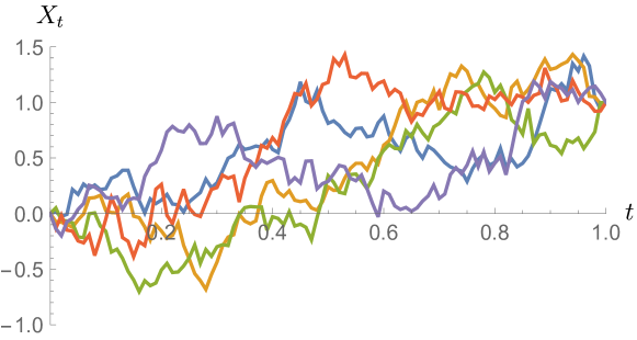
Figure 36: Monte-Carlo simulation of Brownian bridge pinned at $\left(0,0\right)$ and $\left(1,1\right)$, with 5 sample paths.

And it follows in particular that the function on the r.h.s. in eq (457) is a positive definite kernel. Its connection to $F_{2}$ is given in the next lemma.

Now return to the p.d. function $F=F_{2}$; i.e., $F\left(t\right)=1-\left|t\right|$, and therefore, $F\left(s-t\right)=1-\left|s-t\right|$, $s,t\in\left(0,1\right)$, and let $\mathscr{H}_{F}$ be the corresponding RKHS.

Let $\left\{F_{t}\right\}_{t\in\left(0,1\right)}$ denote the kernels in $\mathscr{H}_{F}$, i.e., $\left\langle F_{t},g\right\rangle_{\mathscr{H}_{F}}=g\left(t\right)$, $t\in\left(0,1\right)$, $g\in\mathscr{H}_{F}$. We then have the following:

Lemma 28.11.

Let $\left(X_{t}\right)_{t\in\left(0,1\right)}$ denote the pinned Brownian motion (453); then

$$\left\langle F_{s},F_{t}\right\rangle_{\mathscr{H}_{F}}=Cov\left(X_{s}X_{t}\right);$$ (458)

see (457); and

$$\left\langle F_{s},F_{t}\right\rangle_{energy}=s\wedge t;$$ (459)

while the boundary term

$$bdr\left(s,t\right)=-st.$$ (460)

Proof 28.12.

With our normalization from Figure 36, we must take the energy form as follows:

$$\left\langle f,g\right\rangle_{energy}=\int_{0}^{1}f^{\prime}\left(x\right)g^{\prime}\left(x\right)dx.$$ (461)

Set $F_{s}\left(y\right)=s\wedge y$, see Figure 35. For the distributional derivative we have

$$F_{s}^{\prime}\left(y\right)=\chi_{\left[0,s\right]}\left(y\right)=\begin{cases}1&\mbox{if }0\leq y\leq s\\ 0&\mbox{else},\end{cases}$$

then

$$\left\langle F_{s},F_{t}\right\rangle_{energy} = \int_{0}^{1}F_{s}^{\prime}\left(y\right)F_{t}^{\prime}\left(y\right)dy$$

$$= \int_{0}^{1}\chi_{\left[0,s\right]}\left(y\right)\chi_{\left[0,t\right]}\left(y\right)dy$$

$$= \left|\left[0,s\right]\cap\left[0,t\right]\right|_{\text{Lebesgue measure}}$$

$$= s\wedge t.$$

The desired conclusions (459)-(460) in the lemma now follow. See Remark 28.6.

The verification of (458) uses Ito-calculus Hid (80) as follows: Note that (453) for $X_{t}$ is the solution to the following Ito-equation:

$$dX_{t}=\left(\frac{X_{t}-1}{t-1}\right)dt+dB_{t};$$ (462)

and by Ito’s lemma Hid (80), therefore,

$$\left(dX_{t}\right)^{2}=\left(dB_{t}\right)^{2}.$$ (463)

As a result, if $f:\mathbb{R}\rightarrow\mathbb{R}$ is a function in the energy-Hilbert space defined from (461), then for $0<T<1$, we have,

$$\mathbb{E}\left(\left|f\left(X_{T}\right)\right|^{2}\right)=\mathbb{E}\left(\left|f\left(B_{T}\right)\right|^{2}\right)=\int_{0}^{T}\left|f^{\prime}\left(t\right)\right|^{2}dt=\mathscr{E}_{2}\left(f\right),$$

the energy form of the RKHS (461).     ∎

Remark 28.13.

In (462)-(463), we use standard conventions for Brownian motions $B_{t}$ (see, e.g., Hid (80)): Let $\left(\Omega,\mathscr{F},\mathbb{P}\right)$ be a choice of probability space for $\left\{B_{t}\right\}_{t\in\mathbb{R}}$, (or $t\in\left[0,1\right]$.) With $E\left(\cdots\right)=\int_{\Omega}\cdots d\mathbb{P}$, we have

$$E\left(B_{s}B_{t}\right)=s\wedge t=\min\left(s,t\right),\;t\in\left[0,1\right].$$ (464)

If $f:\mathbb{R}\rightarrow\mathbb{R}$ is a $C^{1}$-function, we write $f\left(B_{t}\right)$ for $f\circ B_{t}$; and $df\left(B_{t}\right)$ refers to Ito-calculus.

28.3 The Case of $F_{3}\left(x\right)=e^{-\left|x\right|}$, $x\in\left(-1,1\right)$

Recall, if $\{B(x)\}_{x\in\mathbb{R}}$ denotes the standard Brownian motion (see, e.g., Sections 3, 20, and 24): then if we set

$$X(x):=e^{-x}B\left(e^{2x}\right),\;x\in\mathbb{R};$$ (465)

then $X\left(x\right)$ is the Ornstein-Uhlenbeck process with

$$\mathbb{E}\left(X\left(x\right)X\left(y\right)\right)=e^{-\left|x-y\right|},\;\forall x,y\in\mathbb{R}.$$ (466)

Let $F_{x}\left(y\right)=F\left(x-y\right)$, for all $x,y\in\left(0,1\right)$; and consider the Hilbert space

$$\mathscr{H}_{F} :=\begin{Bmatrix}h;&\text{continuous on $\left(0,1\right)$, }h\in L^{2}\left(0,1\right)\text{, and}\\ &\text{the weak derivative }h^{\prime}\in L^{2}\left(0,1\right)\,\,\,\,\,\,\,\,\,\,\,\,\,\,\,\end{Bmatrix};$$ (467)

and let the $\mathscr{H}_{F}$-norm, and inner product, be given by

$$\left\|h\right\|_{\mathscr{H}_{F}}^{2}=\frac{1}{2}\left(\int_{0}^{1}\left|h^{\prime}\left(x\right)\right|^{2}dx+\int_{0}^{1}\left|h\left(x\right)\right|^{2}dx\right)+\int_{\partial\Omega}\overline{h_{n}}h\,d\beta.$$ (468)

Here, $d\beta$ on the r.h.s. of (468) denotes the corresponding boundary measure, and $h_{n}$ is the inward normal derivative of $h$. See Theorem 28.16 below.

Then a direct verification yields:

$$\left\langle F_{x},h\right\rangle_{\mathscr{H}_{F}}=h\left(x\right),\;\forall h\in\mathscr{H}_{F},\forall x\in\left(0,1\right);$$ (469)

and it follows that $\mathscr{H}_{F}$ is naturally isomorphic to RKHS for $F_{3}$ (see Section 12).

For details of (469), see also Jør (81).

Corollary 28.14.

In both $\mathscr{H}_{F_{i}}$, $i=2,3$, the deficiency indices are $\left(1,1\right)$.

Proof 28.15.

In both cases, we are referring to the skew-Hermitian operator $D^{\left(F_{i}\right)}$ in $\mathscr{H}_{Fi}$, $i=2,3$; see (438) above. But it follows from (445) and (468) for the respective inner products, that the functions $e^{\pm x}$ have finite positive norms in the respective RKHSs.     ∎

Theorem 28.16.

Let $F=F_{3}$ as before. Consider the energy-Hilbert space

$$\mathscr{H}_{E}:=\begin{Bmatrix}f\in C\left[0,1\right]\,\big{|}\,f,f^{\prime}\in L^{2}\left(0,1\right)\text{ where }\\ f^{\prime}\text{ is the weak derivative of }f\end{Bmatrix}$$ (470)

with

$$\left\langle f,g\right\rangle_{E} =\frac{1}{2}\left(\int_{0}^{1}\overline{f^{\prime}\left(x\right)}g^{\prime}\left(x\right)dx+\int_{0}^{1}\overline{f\left(x\right)}g\left(x\right)dx\right);\;\text{and so}$$ (471)

$$\left\|f\right\|_{E}^{2} =\frac{1}{2}\left(\int_{0}^{1}\left|f^{\prime}\left(x\right)\right|^{2}dx+\int_{0}^{1}\left|f\left(x\right)\right|^{2}dx\right),\;\forall f,g\in\mathscr{H}_{E}.$$ (472)

Set

$$P\left(f,g\right) =\int_{0}^{1}\overline{f_{n}\left(x\right)}g\left(x\right)d\beta\left(x\right),\;\text{where }$$ (473)

$$\beta :=\frac{\delta_{0}+\delta_{1}}{2},\text{ i.e., Dirac masses at endpoints}$$ (474)

where $g_{n}$ denotes the inward normal derivative at endpoints.

Let

$$\mathscr{H}_{F}:=\begin{Bmatrix}f\in C\left[0,1\right]\,\big{|}\,\left\|f\right\|_{E}^{2}+P_{2}\left(f\right)<\infty\text{ where}\\ P_{2}\left(f\right):=P\left(f,f\right)=\int_{0}^{1}\left|f\left(x\right)\right|^{2}d\beta\left(x\right)\end{Bmatrix}$$ (475)

Then we have following:

1. As a Green-Gauss-Stoke principle, we have

   $$\left\|\cdot\right\|_{F}^{2} =\left\|\cdot\right\|_{E}^{2}+P_{2},\;\text{i.e.,}$$ (476)

   $$\left\|f\right\|_{F}^{2} =\left\|f\right\|_{E}^{2}+\int_{0}^{1}\left|f\left(x\right)\right|^{2}d\beta\left(x\right).$$ (477)

2. Moreover,

   $$\left\langle F_{x},g\right\rangle_{E}=g\left(x\right)-\frac{e^{-x}g\left(0\right)+e^{-\left(1-x\right)}g\left(1\right)}{2}.$$ (478)

3. As a result of (478), eq. (476)-(477) is the reproducing property in $\mathscr{H}_{F}$. Specifically, we have

   $$\left\langle F_{x},g\right\rangle_{\mathscr{H}_{F}}=g\left(x\right),\;\forall g\in\mathscr{H}_{F}.\>\text{(see (\ref{eq:en-6}))}$$ (479)

Proof 28.17.

Given $g\in\mathscr{H}_{F}$, one checks directly that

$$P\left(F_{x},g\right) = \int_{0}^{1}F_{x}\left(y\right)g\left(y\right)d\beta\left(y\right)$$

$$= \frac{F_{x}\left(0\right)g\left(0\right)+F_{x}\left(1\right)g\left(1\right)}{2}$$

$$= \frac{e^{-x}g\left(0\right)+e^{-\left(1-x\right)}g\left(1\right)}{2};$$

and, using integration by parts, we have

$$\left\langle F_{x},g\right\rangle_{E} = g\left(x\right)-\frac{e^{-x}g\left(0\right)+e^{-\left(1-x\right)}g\left(1\right)}{2}$$

$$= \left\langle F_{x},g\right\rangle_{F}-P\left(F_{x},g\right).$$

Now, using

$$\int_{\partial\Omega}\left(F_{x}\right)_{n}gd\beta:=\frac{e^{-x}g\left(0\right)+e^{-\left(1-x\right)}g\left(1\right)}{2},$$ (480)

and $\left\langle F_{x},g\right\rangle_{\mathscr{H}_{F}}=g\left(x\right)$, $\forall x\in\left(0,1\right)$, and using (478), the desired conclusion

$$\left\langle F_{x},g\right\rangle_{\mathscr{H}_{F}}=\underset{\text{energy term}}{\underbrace{\left\langle F_{x},g\right\rangle_{E}}}+\int_{\partial\Omega}\left(F_{x}\right)_{n}gd\beta$$ (481)

follows. Since the $\mathscr{H}_{F}$-norm closure of the span of $\left\{F_{x}\>\big{|}\>x\in\left(0,1\right)\right\}$ is all of $\mathscr{H}_{F}$, from (481), we further conclude that

$$\left\langle f,g\right\rangle_{\mathscr{H}_{F}}=\left\langle f,g\right\rangle_{E}+\int_{\partial\Omega}\overline{f_{n}}gd\beta$$ (482)

holds for all $f,g\in\mathscr{H}_{F}$.

In (481) and (482), we used $f_{n}$ to denote the inward normal derivative, i.e., $f_{n}\left(0\right)=f^{\prime}\left(0\right)$, and $f_{n}\left(1\right)=-f^{\prime}\left(1\right)$, $\forall f\in\mathscr{H}_{E}$.     ∎

Example 28.18.

Fix $p$, $0<p\leq 1$, and set

$$F_{p}\left(x\right):=1-\left|x\right|^{p},\;x\in\left(-\tfrac{1}{2},\tfrac{1}{2}\right);$$ (483)

see 37. Then $F_{p}$ is positive definite and continuous; and so $-F^{\prime\prime}_{p}\left(x-y\right)$ is a p.d. kernel, so $-F_{p}^{\prime\prime}$ is a positive definite distribution on $\left(-\frac{1}{2},\frac{1}{2}\right)$.

We saw that if $p=1$, then

$$-F_{1}^{\prime\prime}=2\delta$$ (484)

where $\delta$ is the Dirac mass at $x=0$. But for $0<p<1$, $-F_{p}^{\prime\prime}$ does not have the form (484). We illustrate this if $p=\frac{1}{2}$. Then

$$-F_{\frac{1}{2}}^{\prime\prime}=\chi_{\left\{x\neq 0\right\}}\frac{1}{4}\left|x\right|^{-\frac{3}{2}}+\frac{1}{4}\delta^{\prime\prime},$$ (485)

where $\delta^{\prime\prime}$ is the double derivative of $\delta$ in the sense of distributions.

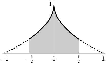
Figure 37: $F_{p}\left(x\right)=1-\left|x\right|^{p}$, $x\in\left(-\tfrac{1}{2},\tfrac{1}{2}\right)$ and $0<p\leq 1$.

Remark 28.19.

There is a notion of boundary measure in potential theory. Boundary measures exist for any potential theory. In our case it works even more generally, whenever p.d. $F_{ex}$ for bounded domains $\Omega\subset\mathbb{R}^{n}$, and even Lie groups. But in the example of $F_{3}$, the boundary is two points.

In all cases, we get $\mathscr{H}_{F}$ as a perturbation of the energy form:

$$\left\|\cdot\right\|_{\mathscr{H}_{F}}^{2}=\text{energy form }+\text{perturbation}$$ (486)

It is a Green-Gauss-Stoke principle. There is still a boundary measure for ALL bounded domains $\Omega\subset\mathbb{R}^{n}$, and even Lie groups.

And RKHS form

$$\left\|\cdot\right\|_{\mathscr{H}_{F}}^{2}=\text{energy form }+\int_{\partial\Omega}f_{n}f\,d\mu_{\text{bd meas.}}$$ (487)

For the general theory of boundary measures and their connection to the Green-Gauss-Stoke principle, we refer readers to JP13a ; JP13b ; Mov (12); Bat (90); Tel (83); ACF (09).

The approach via $\left\|\cdot\right\|_{\mathscr{H}_{F}}^{2}=$ "energy term + boundary term", does not fail to give a RKHS, but we must replace "energy term" with an abstract Dirichlet form; see Refs HS (12); Tre (88).

28.4 Integral Kernels and Positive Definite Functions

Let $0<H<1$ be given, and set

$$K_{H}\left(x,y\right)=\frac{1}{2}\left(\left|x\right|^{2H}+\left|y\right|^{2H}-\left|x-y\right|^{2H}\right),\;\forall x,y\in\mathbb{R}.$$ (488)

It is known that $K_{H}$$\left(\cdot,\cdot\right)$ is the covariance kernel for fractional Brownian motion AJ (12); AJL (11); AL (08); Aur (11). The special case $H=\frac{1}{2}$ is Brownian motion; and if $H=\frac{1}{2}$, then

$$K_{\frac{1}{2}}\left(x,y\right)=\left|x\right|\wedge\left|y\right|=\min\left(\left|x\right|,\left|y\right|\right)$$

if $x$ and $y$ have the same signs. Otherwise the covariance vanishes. See Figure 38.

Set

$$\widetilde{F}_{H}\left(x,y\right) := 1-\left|x-y\right|^{2H}$$

$$F_{H}\left(x\right) := 1-\left|x\right|^{2H}$$

and we recover $F\left(x\right)=1-\left|x\right|\left(=F_{2}\right)$ as a special case of $H=\frac{1}{2}$.

Figure 38: The integral kernel $K_{\frac{1}{2}}\left(x,y\right)=\left|x\right|\wedge\left|y\right|$.

Solving for $F_{H}$ in (488) ($0<H<1$ fixed), we then get

$$F_{H}\left(x-y\right)=\underset{L_{H}}{\underbrace{1-\left|x\right|^{2H}-\left|y\right|^{2H}}}+2K_{H}\left(x,y\right);$$ (489)

and specializing to $x,y\in\left[0,1\right]$; we then get

$$F\left(x-y\right)=\underset{L}{\underbrace{1-x-y}}+2\left(x\wedge y\right);$$

or written differently:

$$K_{F}\left(x,y\right)=L\left(x,y\right)+2E\left(x,y\right)$$ (490)

where $E\left(x,y\right)=x\wedge y$ is the familiar covariance kernel for Brownian motion.

Introducing the Mercer integral kernels corresponding to (489), we therefore get:

$$\left(T_{F_{H}}\varphi\right)\left(x\right) = \int_{0}^{1}\varphi\left(y\right)F_{H}\left(x-y\right)dy$$ (491)

$$\left(T_{L_{H}}\varphi\right)\left(x\right) = \int_{0}^{1}\varphi\left(y\right)L_{H}\left(x,y\right)dy$$ (492)

$$\left(T_{K_{H}}\varphi\right)\left(x\right) = \int_{0}^{1}\varphi\left(y\right)K_{H}\left(x,y\right)dy$$ (493)

for all $\varphi\in L^{2}\left(0,1\right)$, and all $x\in\left[0,1\right]$. Note the special case of (493) for $H=\frac{1}{2}$ is

$$\left(T_{E}\varphi\right)\left(x\right)=\int_{0}^{1}\varphi\left(y\right)\left(x\wedge y\right)\,dy,\;\varphi\in L^{2}\left(0,1\right),x\in\left[0,1\right].$$

We have the following lemma for these Mercer operators:

Lemma 28.20.

Let $0<H<1$, and let $F_{H}$, $L_{H}$ and $K_{H}$ be as in (489), then the corresponding Mercer operators satisfy:

$$T_{F_{H}}=T_{L_{H}}+2T_{K_{H}}.$$ (494)

Proof 28.21.

This is an easy computation, using (489), and (491)-(493).     ∎

28.5 The Ornstein-Uhlenbeck Process Revisited

The reproducing kernel Hilbert space $\mathscr{H}_{F_{2}}$ in (444) is used in computations of Ito-integrals of Brownian motion; while the corresponding RKHS $\mathscr{H}_{F3}$ from (467)-(468) is used in calculations of stochastic integration with the Ornstein-Uhlenbeck process.

Motivated by Newton’s second law of motion, the Ornstein-Uhlenbeck velocity process is proposed to model a random external driving force. In 1D, the process is the solution to the following stochastic differential equation

$$dv_{t}=-\gamma v_{t}dt+\beta dB_{t},\>\gamma,\beta>0.$$ (495)

Here, $-\gamma v_{t}$ is the dissipation, $\beta dB_{t}$ denotes a random fluctuation, and $B_{t}$ is the standard Brownian motion.

Assuming the particle starts at $t=0$. The solution to (495) is a Gaussian stochastic process such that

$$\mathbb{E}\left[v_{t}\right] = v_{0}e^{-\gamma t}$$

$$var\left[v_{t}\right] = \frac{\beta^{2}}{2\gamma}\left(1-e^{-2\gamma t}\right);$$

with $v_{0}$ being the initial velocity. See Figure 39. Moreover, the process has the following covariance function

$$c\left(s,t\right)=\frac{\beta^{2}}{2\gamma}\left(e^{-\gamma\left|t-s\right|}-e^{-\gamma\left|s+t\right|}\right).$$

If we wait long enough, it turns to a stationary process such that

$$c\left(s,t\right)\sim\frac{\beta^{2}}{2\gamma}e^{-\gamma\left|t-s\right|}.$$

This corresponds to the function $F_{3}$. See also Remark 20.7.

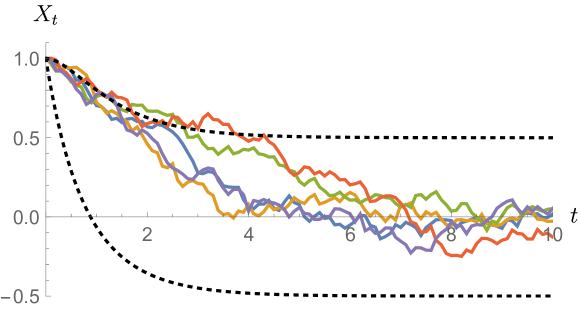
Figure 39: Monte-Carlo simulation of Ornstein-Uhlenbeck process with 5 sample paths. $\beta=\gamma=1$, $v_{0}=1$, $t\in\left[0,10\right]$

28.6 An Overview of the Two Cases: $F_{2}$ and $F_{3}$.

In Table 6 below, we give a list of properties for the particular two cases $F_{2}$ and $F_{3}$ from table 1. Special attention to these examples is merited; first they share a number of properties with much wider families of locally defined positive definite functions; and these properties are more transparent in their simplest form. Secondly, there are important differences between cases $F_{2}$ and $F_{3}$, and the table serves to highlight both differences and similarities. A particular feature that is common for the two is that, when the Mercer operator $T_{F}$ is introduced, then its inverse $T_{F}^{-1}$ exists as an unbounded positive and selfadjoint operator in $\mathscr{H}_{F}$. Moreover, in each case, this operator coincides with the Friedrichs extension of a certain second order Hermitian semibounded operator (calculated from $D^{\left(F\right)}$), with dense domain in $\mathscr{H}_{F}$.

29 Higher Dimensions

Our function above for $F_{3}$ (Sections 28.1 and 28.3) admits a natural extension to $\mathbb{R}^{n}$, $n>1$, as follows.

Let $\Omega\subset\mathbb{R}^{n}$ be a subset satisfying $\Omega\neq\emptyset$, $\Omega$ open and connected; and assume $\overline{\Omega}$ is compact. Let $\triangle=\sum_{i=1}^{n}\left(\partial/\partial x_{i}\right)^{2}$ be the usual Laplacian in $n$-variables.

Lemma 29.1.

Let $F:\Omega-\Omega\rightarrow\mathbb{C}$ be continuous and positive definite; and let $\mathscr{H}_{F}$ be the corresponding RKHS. In $\mathscr{H}_{F}$, we set

$$L^{\left(F\right)}\left(F_{\varphi}\right) :=F_{\triangle\varphi},\;\forall\varphi\in C_{c}^{\infty}\left(\Omega\right),\>\mbox{with}$$ (496)

$$dom\bigl{(}L^{\left(F\right)}\bigr{)} =\left\{F_{\varphi}\>\big{|}\>\varphi\in C_{c}^{\infty}\left(\Omega\right)\right\};$$ (497)

then $L^{\left(F\right)}$ is semibounded in $\mathscr{H}_{F}$, $L^{\left(F\right)}\leq 0$ in the order of Hermitian operators.

Let $T_{F}$ be the Mercer operator; then there is a positive constant $c\>(\>=c_{\left(F,\Omega\right)}>0)$ such that $T_{F}^{-1}$ is a selfadjoint extension of the densely defined operator $c\left(I-L^{\left(F\right)}\right)$ in $\mathscr{H}_{F}$.

Proof 29.2.

The ideas for the proof are contained in Sections 28.1 and 28.3 above. To get the general conclusions, we may combine these considerations with the general theory of Green’s functions for elliptic linear PDEs (partial differential equations); see also Nel (57); JLW (69).     ∎

1. $F_{2}\left(x\right)=1-\left|x\right|$, $\left|x\right|<\frac{1}{2}$ 2. Mercer operator $$T_{F_{2}}:L^{2}\left(0,\tfrac{1}{2}\right)\rightarrow L^{2}\left(0,\tfrac{1}{2}\right)$$ 3. $T_{F_{2}}^{-1}$ is unbounded, selfadjoint Proof 29.3. Since $T_{F}$ is positive, bounded, and trace class, it follows that $T_{F_{2}}^{-1}$ is positive, unbounded, and selfadjoint.     ∎ 4. $T_{F_{2}}^{-1}=$ Friedrichs extension of $$-\tfrac{1}{2}\bigl{(}\tfrac{d}{dx}\bigr{)}^{2}\Big{|}_{C_{c}^{\infty}\left(0,\frac{1}{2}\right)}$$ as a selfadjoint operator on $L^{2}\left(0,\frac{1}{2}\right)$. Sketch of proof. Setting $$u\left(x\right)=\int_{0}^{\frac{1}{2}}\varphi\left(y\right)\left(1-\left|x-y\right|\right)dy$$ then $\displaystyle u^{\prime\prime}$ $\displaystyle=$ $\displaystyle-2\varphi$ $\displaystyle\Updownarrow$ $\displaystyle u$ $\displaystyle=$ $\displaystyle\left(-\tfrac{1}{2}\bigl{(}\tfrac{d}{dx}\bigr{)}^{2}\right)^{-1}\varphi$ and so $$T_{F_{2}}=\left(-\tfrac{1}{2}\bigl{(}\tfrac{d}{dx}\bigr{)}^{2}\right)^{-1}.$$ And we get a selfadjoint extension $$T_{F_{2}}^{-1}\supset-\tfrac{1}{2}\bigl{(}\tfrac{d}{dx}\bigr{)}^{2}$$ in $L^{2}\left(0,\frac{1}{2}\right)$, where the containment refers to operator graphs.

1. $F_{3}\left(x\right)=e^{-\left|x\right|}$, $\left|x\right|<1$ 2. Mercer operator $$T_{F_{3}}:L^{2}\left(0,1\right)\rightarrow L^{2}\left(0,1\right)$$ 3. $T_{F_{3}}^{-1}$ is unbounded, selfadjoint Proof 29.4. Same argument as in the proof for $T_{F_{2}}^{-1}$; also follows from Mercer’s theorem.     ∎ 4. $T_{F_{2}}^{-1}=$ Friedrichs extension of $$\tfrac{1}{2}\bigl{(}I-\bigl{(}\tfrac{d}{dx}\bigr{)}^{2}\bigr{)}\Big{|}_{C_{c}^{\infty}\left(0,1\right)}$$ as a selfadjoint operator on $L^{2}\left(0,1\right)$. Sketch of proof. Setting $$u\left(x\right)=\int_{0}^{1}\varphi\left(y\right)e^{-\left|x-y\right|}dy$$ then $\displaystyle u^{\prime\prime}$ $\displaystyle=$ $\displaystyle u-2\varphi$ $\displaystyle\Updownarrow$ $\displaystyle u$ $\displaystyle=$ $\displaystyle\left(\tfrac{1}{2}\bigl{(}1-\bigl{(}\tfrac{d}{dx}\bigr{)}^{2}\bigr{)}\right)^{-1}\varphi$ and so $$T_{F_{3}}=\left(\tfrac{1}{2}\left(I-\bigl{(}\tfrac{d}{dx}\bigr{)}^{2}\right)\right)^{-1}.$$ Now, a selfadjoint extension $$T_{F_{3}}^{-1}\supset\tfrac{1}{2}\left(I-\bigl{(}\tfrac{d}{dx}\bigr{)}^{2}\right)$$ in $L^{2}\left(0,1\right)$.

Table 6: An overview of two cases: $F_{2}$ v.s. $F_{3}$.

Chapter 8 Comparing the Different RKHSs $\mathscr{H}_{F}$ and $\mathscr{H}_{K}$

In the earlier chapters we have studied extension problems for particular locally defined positive definite functions $F$. In each case, the p.d. function $F$ was fixed. Many classes of p.d. functions were studied but not compared. Indeed, the cases we studied have varied between different levels of generality, and varied between cases separated by different technical assumptions. All our results, in turn, have been motivated by explicit applications.

In the present chapter, we turn to a comparison between the results we obtain for pairs of locally defined positive definite functions. We answer such questions as this: Given an open domain $\Omega$ (in an ambient group $G$), and two continuous positive functions $F$ and $K$, both defined on $\Omega^{-1}\Omega$, how do the two associated RKHSs compare? (Theorem 29.12.) How to compare spectral theoretic information for the two? How does the operator theory compare, for the associated pair of skew-Hermitian operators $D^{\left(F\right)}$ and $D^{\left(K\right)}$? (Theorem 30.1.) What if $F$ is fixed, and $K$ is taken to be the complex conjugate of $F$? Theorem 32.6.) What are the properties of the imaginary part of $F$? (Section 33.)

Before we turn to comparison of pairs of RKHSs, we will prove a lemma which accounts for two uniformity principles for positive definite continuous functions defined on open subsets in locally compact groups:

Lemma 29.5.

Let $G$ be a locally compact group, and let $\Omega\subset G$ be an open and connected subset, $\Omega\neq\emptyset$. Let $F:\Omega^{-1}\Omega\rightarrow\mathbb{C}$ be a continuous positive definite function satisfying $F\left(e\right)=1$, where $e\in G$ is the unit for the group operation.

1. Then $F$ extends by limit to a continuous p.d. function

   $$F^{\left(ex\right)}:\overline{\Omega}^{-1}\overline{\Omega}\longrightarrow\mathbb{C}.$$ (498)

2. Moreover, the two p.d. functions $F$ and $F^{\left(ex\right)}$ have the same RKHS consisting of continuous functions $\xi$ on $\overline{\Omega}$ such that, $\exists\,0<A<\infty$, $A=A_{\xi}$, s.t.

   $$\left|\int_{\overline{\Omega}}\overline{\xi\left(x\right)}\varphi\left(x\right)dx\right|^{2}\leq A\left\|F_{\varphi}\right\|_{\mathscr{H}_{F}}^{2},\;\forall\varphi\in C_{c}\left(\Omega\right)$$ (499)

   where $dx=$ Haar measure on $G$,

   $$F_{\varphi}\left(\cdot\right)=\int_{\Omega}\varphi\left(y\right)F\left(y^{-1}\cdot\right)dy,\;\varphi\in C_{c}\left(\Omega\right);$$

   and $\left\|F_{\varphi}\right\|_{\mathscr{H}_{F}}$ denotes the $\mathscr{H}_{F}$-norm of $F_{\varphi}$.

3. Every $\xi\in\mathscr{H}_{F}$ satisfies the following a priori estimate:

   $$\left|\xi\left(x\right)-\xi\left(y\right)\right|^{2}\leq 2\left\|\xi\right\|_{\mathscr{H}_{F}}^{2}\left(1-\Re\left\{F\left(x^{-1}y\right)\right\}\right)$$ (500)

   for all $\xi\in\mathscr{H}_{F}$, and all $x,y\in\overline{\Omega}$.

Proof 29.6.

The arguments in the proof only use standard tools from the theory of reproducing kernel Hilbert spaces. We covered a special case in Section 24, and so we omit the details here.     ∎

Now add the further assumption on the subset $\Omega\subset G$ from the lemma: Assume in addition that $\Omega$ has compact closure, so $\overline{\Omega}$ is compact. Let $\partial\Omega=\overline{\Omega}\backslash\Omega$ be the boundary. With this assumption, we get automatically the inclusion

$$C\left(\overline{\Omega}\right)\subset L^{2}\left(\overline{\Omega}\right)$$

since continuous functions on $\overline{\Omega}$ are automatically uniformly bounded, and Haar measure on $G$ has the property that $\left|\overline{\Omega}\right|<\infty$.

Definition 29.7.

Let $\left(\Omega,F\right)$ be as above, i.e.,

$$F:\overline{\Omega}^{-1}\overline{\Omega}\longrightarrow\mathbb{C}$$

is continuous and positive definite. Assume $G$ is a Lie group. Recall, extension by limit to $\overline{\Omega}$ is automatic by the limit. Let $\beta\in\mathscr{M}\left(\partial\Omega\right)$ be a positive finite measure on the boundary $\partial\Omega$. We say that $\beta$ is a boundary measure iff

$$\left\langle T_{F}f,\xi\right\rangle_{\mathscr{H}_{F}}-\int_{\Omega}\overline{f\left(x\right)}\xi\left(x\right)dx=\int_{\partial\Omega}\overline{\left(T_{F}f\right)_{n}\left(\sigma\right)}\xi\left(\sigma\right)d\beta\left(\sigma\right)$$ (501)

holds for all $f\in C\left(\overline{\Omega}\right)$, $\forall\xi\in\mathscr{H}_{F}$, where $\left(\cdot\right)_{n}=$ normal derivative computed on the boundary $\partial\Omega$ of $\Omega$.

Remark 29.8.

For the example $G=\mathbb{R}$, $\overline{\Omega}=\left[0,1\right]$, $\partial\Omega=\left\{0,1\right\}$, and $F=F_{3}$ on $\left[0,1\right]$, where

$$F\left(x\right)=e^{-\left|x\right|},\;\forall x\in\left[-1,1\right],$$

the boundary measure is

$$\beta=\frac{1}{2}\left(\delta_{0}+\delta_{1}\right).$$ (502)

Let $G$ be a locally compact group with left-Haar measure, and let $\Omega\subset G$ be a non-empty subset satisfying: $\Omega$ is open and connected; and is of finite Haar measure; write $\left|\Omega\right|<\infty$. The Hilbert space $L^{2}\left(\Omega\right)=L^{2}\left(\Omega,dx\right)$ is the usual $L^{2}$-space of measurable functions $f$ on $\Omega$ such that

$$\left\|f\right\|_{L^{2}\left(\Omega\right)}^{2}:=\int_{\Omega}\left|f\left(x\right)\right|^{2}dx<\infty.$$ (503)

Definition 29.9.

Let $F$ and $K$ be two continuous and positive definite functions defined on

$$\Omega^{-1}\cdot\Omega:=\left\{x^{-1}y\>\Big{|}\>x,y\in\Omega\right\}.$$ (504)

We say that $K\ll F$ iff there is a finite constant $A$ such that for all finite subsets $\left\{x_{i}\right\}_{i=1}^{N}\subset\Omega$, and all systems $\left\{c_{i}\right\}_{i=1}^{N}\subset\mathbb{C}$, we have:

$$\sum_{i}\sum_{j}\overline{c_{i}}c_{j}K\left(x_{i}^{-1}x_{j}\right)\leq A\sum_{i}\sum_{j}\overline{c_{i}}c_{j}F\left(x_{i}^{-1}x_{j}\right).$$ (505)

Lemma 29.10.

Let $F$ and $K$ be as above; then $K\ll F$ if and only if there is a finite constant $A\in\mathbb{R}_{+}$ such that

$$\int_{\Omega}\int_{\Omega}\overline{\varphi\left(x\right)}\varphi\left(y\right)K\left(x^{-1}y\right)dxdy\leq A\int_{\Omega}\int_{\Omega}\overline{\varphi\left(x\right)}\varphi\left(y\right)F\left(x^{-1}y\right)dxdy$$ (506)

holds for all $\varphi\in C_{c}\left(\Omega\right)$. The constant $A$ in (505) and (506) will be the same.

Proof 29.11.

Easy; use an approximate identity in $G$, see e.g., Rud (73, 90).     ∎

Setting

$$F_{\varphi}\left(x\right)=\int_{\Omega}\varphi\left(y\right)F\left(y^{-1}x\right)dy,$$ (507)

and similarly for $K_{\varphi}=\int_{\Omega}\varphi\left(y\right)K\left(y^{-1}\cdot\right)dy$, we note that $K\ll F$ if and only if:

$$\left\|K_{\varphi}\right\|_{\mathscr{H}_{K}}\leq\sqrt{A}\left\|F_{\varphi}\right\|_{\mathscr{H}_{F}},\;\forall\varphi\in C_{c}\left(\Omega\right).$$ (508)

Further, note that, if $G$ is also a Lie group, then (508) follows from checking it only for all $\varphi\in C_{c}^{\infty}\left(G\right)$. See Lemma 10.12.

Theorem 29.12.

Let $\Omega$, $F$ and $K$ be as in Definition 29.9, i.e., both continuous and p.d. on the set $\Omega^{-1}\cdot\Omega$ in (504); then the following two conditions are equivalent:

1. $K\ll F$, and

2. $\mathscr{H}_{K}$ is a closed subspace of $\mathscr{H}_{F}$.

Proof 29.13.

$\Downarrow$ Assume $K\ll F$, we then define a linear operator $l:\mathscr{H}_{F}\rightarrow\mathscr{H}_{K}$, setting

$$l\left(F_{\varphi}\right):=K_{\varphi},\;\forall\varphi\in C_{c}\left(\Omega\right).$$ (509)

We now use (508), plus the fact that $\mathscr{H}_{F}$ is the $\left\|\cdot\right\|_{\mathscr{H}_{F}}$-completion of

$$\left\{F_{\varphi}\>\Big{|}\>\varphi\in C_{c}\left(\Omega\right)\right\};$$

and similarly for $\mathscr{H}_{K}$.

As a result of (509) and (508), we get a canonical extension of $l$ to a bounded linear operator, also denoted $l:\mathscr{H}_{F}\rightarrow\mathscr{H}_{K}$, and

$$\left\|l\left(\xi\right)\right\|_{\mathscr{H}_{K}}\leq\sqrt{A}\left\|\xi\right\|_{\mathscr{H}_{F}},\mbox{ for all }\xi\in\mathscr{H}_{F}.$$ (510)

We interrupt the proof to give a lemma:     ∎

Lemma 29.14.

Let $F$, $K$, $\Omega$ be as above. Assume $K\ll F$, and let $l:\mathscr{H}_{F}\rightarrow\mathscr{H}_{K}$ be the bounded operator introduced in (509) and (510). Then the adjoint operator $l^{*}:\mathscr{H}_{K}\rightarrow\mathscr{H}_{F}$ satisfies:

$$\left(l^{*}\left(\xi\right)\right)\left(x\right)=\xi\left(x\right),\mbox{ for all }\xi\in\mathscr{H}_{K},x\in\Omega.$$ (511)

And of course, $l^{*}\left(\xi\right)\in\mathscr{H}_{F}$.

Proof 29.15.

By the definite of $l^{*}$, as the adjoint of a bounded linear operator between Hilbert spaces, we get

$$\left\|l^{*}\right\|_{\mathscr{H}_{K}\rightarrow\mathscr{H}_{F}}=\left\|l\right\|_{\mathscr{H}_{F}\rightarrow\mathscr{H}_{K}}\leq\sqrt{A}$$ (512)

for the respective operator norms; and

$$\left\langle l^{*}\left(\xi\right),F_{\varphi}\right\rangle_{\mathscr{H}_{F}}=\left\langle\xi,K_{\varphi}\right\rangle_{\mathscr{H}_{K}},\;\forall\varphi\in C_{c}\left(\Omega\right).$$ (513)

Using now the reproducing property in the two RKHSs, we get:

$$l.h.s.\left(\ref{eq:FK-11}\right) = \int_{\Omega}\overline{l^{*}\left(\xi\right)\left(x\right)}\varphi\left(x\right)dx,\mbox{ and}$$

$$r.h.s.\left(\ref{eq:FK-11}\right) = \int_{\Omega}\overline{\xi\left(x\right)}\varphi\left(x\right)dx,\;\mbox{ for all }\varphi\in C_{c}\left(\Omega\right).$$

Taking now approximations in $C_{c}\left(\Omega\right)$ to the Dirac masses $\{\delta_{x}\>|\>x\in\Omega\}$, the desired conclusion (511) follows.     ∎

Proof 29.16.

(of Theorem 29.12 continued.) Assume $K\ll F$, the lemma proves that $\mathscr{H}_{K}$ identifies with a linear space of continuous functions $\xi$ on $\Omega$, and if $\xi\in\mathscr{H}_{K}$, then it is also in $\mathscr{H}_{F}$.

We claim that this is a closed subspace in $\mathscr{H}_{F}$ relative to the $\mathscr{H}_{F}$-norm.

Step 1. Let $\left\{\xi_{n}\right\}\subset\mathscr{H}_{K}$ satisfying

$$\lim_{n,m\rightarrow\infty}\left\|\xi_{n}-\xi_{m}\right\|_{\mathscr{H}_{F}}=0.$$

By (510) and (511), the lemma; we get

$$\lim_{n,m\rightarrow\infty}\left\|\xi_{n}-\xi_{m}\right\|_{\mathscr{H}_{K}}=0.$$

Step 2. Since $\mathscr{H}_{K}$ is complete, we get $\chi\in\mathscr{H}_{K}$ such that

$$\lim_{n\rightarrow\infty}\left\|\xi_{n}-\chi\right\|_{\mathscr{H}_{K}}=0.$$ (514)

Step 3. We claim that this $\mathscr{H}_{K}$-limit $\chi$ also defines a unique element in $\mathscr{H}_{F}$, and it is therefore the $\mathscr{H}_{F}$-limit.

We have for all $\varphi\in C_{c}\left(\Omega\right)$:

$$\left|\int_{\Omega}\overline{\chi\left(x\right)}\varphi\left(x\right)dx\right| \leq \left\|\chi\right\|_{\mathscr{H}_{K}}\left\|K_{\varphi}\right\|_{\mathscr{H}_{K}}$$

$$\leq \left\|\chi\right\|_{\mathscr{H}_{K}}\sqrt{A}\left\|F_{\varphi}\right\|_{\mathscr{H}_{F}};$$

and so $\chi\in\mathscr{H}_{F}$.

We now turn to the converse implication of Theorem 29.12:

$\Uparrow$ Assume $F$ and $K$ are as in the statement of the theorem; and that $\mathscr{H}_{K}$ is a close subspace in $\mathscr{H}_{F}$ via identification of the respective continuous functions on $\Omega$. We then prove that $K\ll F$.

Now let $P_{K}$ denote the orthogonal projection of $\mathscr{H}_{F}$ onto the closed subspace $\mathscr{H}_{K}$. We claim that

$$P_{K}\left(F_{\varphi}\right)=K_{\varphi},\;\forall\varphi\in C_{c}\left(\Omega\right).$$ (515)

Using the uniqueness of the projection $P_{K}$, we need to verify that $F_{\varphi}-K_{\varphi}\in\mathscr{H}_{F}\ominus\mathscr{H}_{K}$; i.e., that

$$\left\langle F_{\varphi}-K_{\varphi},\xi_{K}\right\rangle_{\mathscr{H}_{F}}=0,\;\mbox{for all }\xi_{K}\in\mathscr{H}_{K}.$$ (516)

But since $\mathscr{H}_{K}\subset\mathscr{H}_{F}$, we have

$$l.h.s.\left(\ref{eq:FK-14}\right)=\int_{\Omega}\overline{\varphi\left(x\right)}\xi_{K}\left(x\right)dx-\int_{\Omega}\overline{\varphi\left(x\right)}\xi_{K}\left(x\right)dx=0,$$

for all $\varphi\in C_{c}\left(\Omega\right)$. This proves (515).

To verify $K\ll F$, we use the criterion (508) from Lemma 29.10. Indeed, consider $K_{\varphi}\in\mathscr{H}_{K}$. Since $\mathscr{H}_{K}\subset\mathscr{H}_{F}$, we get

$$l\left(F_{\varphi}\right)=P_{K}\left(F_{\varphi}\right)=K_{\varphi},\;\mbox{and}$$

$$\left\|K_{\varphi}\right\|_{\mathscr{H}_{K}}=\left\|l\left(F_{\varphi}\right)\right\|_{\mathscr{H}_{K}}\leq\sqrt{A}\left\|F_{\varphi}\right\|_{\mathscr{H}_{F}}$$

which is the desired estimate (508).     ∎

Example 29.17.

To illustrate the conclusion in Theorem 29.12, take

$$K\left(x\right)=\left(\frac{\sin x}{x}\right)^{2},\;\mbox{and }F\left(x\right)=\frac{1}{1+x^{2}};$$ (517)

both defined on the fixed interval $-\frac{1}{4}<x<\frac{1}{4}$; and so the interval for $\Omega$ in both cases can be take to be $\Omega=\left(0,\frac{1}{4}\right)$; compare with $F_{4}$ and $F_{1}$ from Table 1.

Claim 4.

$K\ll F$, and $\mathscr{H}_{K}\subseteq\mathscr{H}_{F}$.

Proof 29.18.

Using Table 2, we can identify measures $\mu_{K}\in Ext\left(K\right)$, and $\mu_{F}\in Ext\left(F\right)$. With the use of Corollary 7.10, and Corollary 12.15, it is now easy to prove that $K\ll F$; i.e., that condition (i) in Theorem 29.12 is satisfied. Also, recall from Lemma 7.4 that the RKHSs are generated by the respective kernels, i.e., the functions $K$ and $F$:

For $x_{0}\in\left[0,\frac{1}{4}\right]=\overline{\Omega}$, set

$$K_{x_{0}}\left(y\right)=\left(\frac{\sin\left(y-x_{0}\right)}{y-x_{0}}\right)^{2},\quad y\in\Omega.$$ (518)

To show directly that $\mathscr{H}_{K}$ is a subspace of $\mathscr{H}_{F}$, we use Corollary 7.10: We find a signed measure $v_{x_{0}}\in\mathfrak{M}_{2}\left(F,\Omega\right)$ such that

$$K_{x_{0}}\left(\cdot\right)=\left(v_{v_{0}}*F\right)\left(\cdot\right)\;\mbox{on $\Omega$ holds.}$$ (519)

The r.h.s. in (519) is short hand for

$$K_{x_{0}}\left(x\right)=\int_{0}^{\frac{1}{4}}\left(\frac{1}{1+\left(x-y\right)^{2}}d\nu_{x_{0}}\left(y\right)\right),$$ (520)

using Fourier transform, eq (520) is easily solved by the signed measure $v_{x_{0}}$ s.t.

$$\widehat{dv_{0}}\left(\lambda\right)=\chi_{\left[-\frac{1}{2},\frac{1}{2}\right]}\left(\lambda\right)\left(1-2\left|\lambda\right|\right)e^{\left|\lambda\right|}e^{ix_{0}\lambda}d\lambda.$$ (521)

Note that the r.h.s. in (521) is of compact support; and so an easy Fourier inversion then yields the signed measure $v_{x_{0}}\in\mathfrak{M}_{2}\left(F,\Omega\right)$ which solves eq (519). Hence $K_{x_{0}}\left(\cdot\right)\in\mathscr{H}_{F}$; and so $\mathscr{H}_{K}$ is a subspace of $\mathscr{H}_{F}$.     ∎

30 Applications

Below we give an application of Theorem 29.12 to the deficiency-index problem, and to the computation of the deficiency spaces; see also Lemma 18.9, and Lemma 35.1.

As above, we will consider two given continuous p.d. functions $F$ and $K$, but the group now is $G=\mathbb{R}$: We pick $a,b\in\mathbb{R}_{+}$, $0<a<b$, such that $F$ is defined on $\left(-b,b\right)$, and $K$ on $\left(-a,a\right)$. The corresponding two RKHSs will be denoted $\mathscr{H}_{F}$ and $\mathscr{H}_{K}$. We say that $K\ll F$ iff there is a finite constant $A$ such that

$$\left\|K_{\varphi}\right\|_{\mathscr{H}_{K}}^{2}\leq A\left\|F_{\varphi}\right\|_{\mathscr{H}_{F}}^{2}$$ (522)

for all $\varphi\in C_{c}\left(0,a\right)$. Now this is a slight adaptation of our Definition 29.9 above, but this modification will be needed; for example in computing the indices of two p.d. functions $F_{2}$ and $F_{3}$ from Table 1; see also Section 28 below. In fact, a simple direct checking shows that

$$F_{2}\ll F_{3}\quad\left(\mbox{see Table }\ref{tab:F1-F6}\right),$$ (523)

and we now take $a=\frac{1}{2}$, $b=1$.

Here, $F_{2}\left(x\right)=1-\left|x\right|$ in $\left|x\right|<\frac{1}{2}$; and $F_{3}\left(x\right)=e^{-\left|x\right|}$ in $\left|x\right|<1$; see Figure 40.

(a) $F_{2}\left(x\right)=1-\left|x\right|$, $\left|x\right|<\frac{1}{2}$

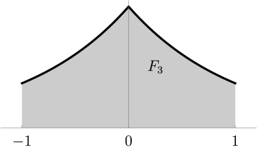
(b) $F_{3}\left(x\right)=e^{-\left|x\right|}$, $\left|x\right|<1$

Figure 40: The examples of $F_{2}$ and $F_{3}$.

We wish to compare the respective skew-Hermitian operators, $D^{\left(F\right)}$ in $\mathscr{H}_{F}$; and $D^{\left(F\right)}$ in $\mathscr{H}_{K}$ (Section 14), i.e.,

$$D^{\left(F\right)}\left(F_{\varphi}\right) = F_{\varphi^{\prime}},\;\forall\varphi\in C_{c}^{\infty}\left(0,b\right);\;\mbox{and}$$ (524)

$$D^{\left(K\right)}\left(K_{\varphi}\right) = K_{\varphi^{\prime}},\;\forall\varphi\in C_{c}^{\infty}\left(0,a\right).$$ (525)

Let $z\in\mathbb{C}$; and we set

$$DEF_{F}\left(z\right) = \left\{\xi\in dom\bigl{(}\bigl{(}D^{\left(F\right)}\bigr{)}^{*}\bigr{)}\>\Big{|}\>\bigl{(}D^{\left(F\right)}\bigr{)}^{*}\xi=z\xi\right\},\;\mbox{and}$$ (526)

$$DEF_{K}\left(z\right) = \left\{\xi\in dom\bigl{(}\bigl{(}D^{\left(K\right)}\bigr{)}^{*}\bigr{)}\>\Big{|}\>\bigl{(}D^{\left(K\right)}\bigr{)}^{*}\xi=z\xi\right\}.$$ (527)

Theorem 30.1.

Let two continuous p.d. functions $F$ and $K$ be specified as above, and suppose

$$K\ll F;$$ (528)

then

$$DEF_{K}\left(z\right)=DEF_{F}\left(z\right)\Big{|}_{\left(0,a\right)}$$ (529)

i.e., restriction to the smaller interval.

Proof 30.2.

Since (528) is assumed, it follows from Theorem 29.12, that $\mathscr{H}_{K}$ is a subspace of $\mathscr{H}_{F}$.

If $\varphi\in C_{c}^{\infty}\left(0,b\right)$, and $\xi\in dom\bigl{(}\bigl{(}D^{\left(F\right)}\bigr{)}^{*}\bigr{)}$, then

$$\left\langle\bigl{(}D^{\left(F\right)}\bigr{)}^{*}\xi,F_{\varphi}\right\rangle_{\mathscr{H}_{F}}=\left\langle\xi,F_{\varphi^{\prime}}\right\rangle_{\mathscr{H}_{F}}=\int_{0}^{b}\overline{\xi\left(x\right)}\varphi^{\prime}\left(x\right)dx;$$

and it follows that functions $\xi$ in $DEF_{F}\left(z\right)$ must be multiples of

$$\left(0,b\right)\ni x\longmapsto e_{z}\left(x\right)=e^{-zx}.$$ (530)

Hence, by Theorem 29.12, we get

$$DEF_{K}\left(z\right)\subseteq DEF_{F}\left(z\right),$$

and by (530), we see that(529) must hold.

Conversely, if $DEF_{F}\left(z\right)\neq 0$, then $l\left(DEF_{F}\left(z\right)\right)\neq 0$, and its restriction to $\left(0,a\right)$ is contained in $DEF_{K}\left(z\right)$. The conclusion in the theorem follows.     ∎

Remark 30.3.

The spaces $DEF_{\left(F\right)}\left(z\right)$, $z\in\mathbb{C}$, are also discussed in Theorem 11.3.

Example 30.4 (Application).

Consider the two functions $F_{2}$ and $F_{3}$ in Table 1. Both of the operators $D^{\left(F_{i}\right)}$, $i=2,3$, have deficiency indices $\left(1,1\right)$.

Proof 30.5.

One easily checks that $F_{2}\ll F_{3}$. And it is also easy to check directly that $D^{\left(F_{2}\right)}$ has indices $\left(1,1\right)$. Hence, by (529) in the theorem, it follows that $D^{\left(F_{3}\right)}$ also must have indices $\left(1,1\right)$. (The latter conclusion is not as easy to verify by direct means!)     ∎

31 Radially Symmetric Positive Definite Functions

Among other subclasses of positive definite functions we have radially symmetric p.d. functions. If a given p.d. function happens to be radially symmetric, then there are a number of simplifications available, and the analysis in higher dimension often simplifies. This is to a large extend due to theorems of I. J. Schöenberg and D. V. Widder. Below we sketch two highpoints, but we omit details and application to interpolation and to geometry. These themes are in the literature, see e.g. Sch38c ; SW (53); Sch (64); Wid (41); WW (75).

Remark 31.1.

In some cases, the analysis in one dimension yields insight into the possibilities in $\mathbb{R}^{n}$, $n>1$. This leads for example for functions $F$ on $\mathbb{R}^{n}$ which are radial, i.e., of the form $F\left(x\right)=\Phi\bigl{(}\left\|x\right\|^{2}\bigr{)}$, where $\left\|x\right\|^{2}=\sum_{i=1}^{n}x_{i}^{2}$.

A function $q$ on $\mathbb{R}_{+}$, $q:\mathbb{R}_{+}\rightarrow\mathbb{R}$, is said to be completely monotone iff $q\in C\left(\left[0,\infty\right)\right)\cap C^{\infty}\left(\left(0,\infty\right)\right)$ and

$$\left(-1\right)^{n}q^{\left(n\right)}\left(r\right)\geq 0,\;r\in\mathbb{R}_{+},n\in\mathbb{N}_{0}.$$ (531)

Example 31.2.

$$q\left(r\right) = e^{-\alpha r},\qquad\alpha\geq 0;$$

$$q\left(r\right) = \frac{\alpha}{r^{1-\alpha}},\qquad\alpha\leq 1;$$

$$q\left(r\right) = \frac{1}{\left(r+\alpha^{2}\right)^{\beta}},\;\alpha>0,\beta\geq 0.$$

Theorem 31.3 (Schöenberg (1938) ).

A function $q:\mathbb{R}_{+}\rightarrow\mathbb{R}$ is completely monotone iff the corresponding function $F_{q}\left(x\right)=q\bigl{(}\left\|x\right\|^{2}\bigr{)}$ is positive definite and radial on $\mathbb{R}^{n}$ for all $k\in\mathbb{N}$.

Proof 31.4.

See, e.g., BCR (84); Sch38a ; Sch38b . We omit details, but the proof uses:     ∎

Theorem 31.5 (Bernstein-Widder ).

A function $q:\mathbb{R}_{+}\rightarrow\mathbb{R}$ is completely monotone iff there is a finite positive Borel measure on $\mathbb{R}_{+}$ s.t.

$$q\left(r\right)=\int_{0}^{\infty}e^{-rt}d\mu\left(t\right),\;r\in\mathbb{R}_{+},$$

i.e., $q$ is the Laplace transform of a finite positive measure $\mu$ on $\mathbb{R}_{+}$.

Proof 31.6.

See, e.g., BCR (84); Wid (41); Ber (46, 29); Wid (64); BW (40).     ∎

Remark 31.7.

The condition that the function $q$ in (531) be in $C^{\infty}\left(\mathbb{R}_{+}\right)$ may be relaxed; and then (531) takes the following alternative form:

$$\sum_{k=1}^{n}\left(-1\right)^{k}\binom{n}{k}q\left(r+k\delta\right)\geq 0$$ (532)

for all $n\in\mathbb{N}$, all $\delta>0$, and $x\in\bigl{[}0,\infty\bigr{)}$; i.e.,

$$q\left(r\right)-q\left(r+\delta\right)\geq 0$$

$$q\left(r\right)-2q\left(r+\delta\right)+q\left(r+2\delta\right)\geq 0\;\;\mbox{e.t.c. }$$

It is immediate that every completely monotone function $q$ on $\bigl{[}0,\infty\bigr{)}$ is convex.

Remark 31.8.

A related class of functions $q:\mathbb{R}_{+}\rightarrow\mathbb{R}$ is called $\Phi_{n}$; the functions $q$ such that $\mathbb{R}^{n}\ni x\longmapsto q\left(\left\|x\right\|\right)$ is positive definite on $\mathbb{R}^{n}$. Schönberg Sch38a showed that $q\in\Phi_{n}$ if and only if there is a finite positive Borel measure $\mu$ on $\mathbb{R}_{+}$ such that

$$q\left(r\right)=\int_{0}^{\infty}\Omega_{n}\left(rt\right)d\mu\left(t\right)$$ (533)

where

$$\Omega_{n}\left(s\right)=\Gamma\left(\frac{n}{2}\right)\left(\frac{2}{s}\right)^{\frac{n-2}{2}}J_{\frac{n-2}{2}}\left(s\right)=\sum_{j=0}^{\infty}\left(-\frac{s^{2}}{4}\right)^{j}\frac{\Gamma\left(\frac{n}{2}\right)}{j!\Gamma\left(\frac{n}{2}+j\right)}.$$

Indeed, if $\nu_{n}$ denotes the normalized uniform measure on $S:=\left\{x\in\mathbb{R}^{n}\>|\>\left\|x\right\|=1\right\}$, then

$$\Omega_{n}\left(\left\|x\right\|\right)=\int_{S}e^{ix\cdot y}d\nu_{n}\left(y\right),\quad\forall x\in\mathbb{R}^{n}.$$

32 Connecting $F$ and $\overline{F}$ When $F$ is a Positive Definite Function

Let $F:\left(-1,1\right)\rightarrow\mathbb{C}$ be continuous and positive definite, and let $\overline{F}$ be the complex conjugate, i.e., $\overline{F}$$\left(x\right)=F\left(-x\right)$, $\forall x\in\left(-1,1\right)$. Below, we construct a contractive-linking operator $\mathscr{H}_{F}\rightarrow\mathscr{H}_{\overline{F}}$ between the two RKHSs.

Lemma 32.1.

Let $\mu$ and $\mu^{\left(s\right)}$ be as before, $\mu^{\left(s\right)}=\mu\circ s$, $s\left(x\right)=-x$; and set

$$g=\sqrt{\frac{d\mu^{\left(s\right)}}{d\mu}};$$ (534)

(the square root of the Radon-Nikodym derivative) then the $g$-multiplication operator is isometric between the respective Hilbert spaces; $L^{2}\left(\mu^{\left(s\right)}\right)$ and $L^{2}\left(\mu\right)$ as follows:

$$\lx@xy@svg{\hbox{\raise 0.0pt\hbox{\kern 24.09747pt\hbox{\ignorespaces\ignorespaces\ignorespaces\hbox{\vtop{\kern 0.0pt\offinterlineskip\halign{\entry@#!@&&\entry@@#!@\cr&&\crcr}}}\ignorespaces{\hbox{\kern-24.09747pt\raise 0.0pt\hbox{\hbox{\kern 0.0pt\raise 0.0pt\hbox{\hbox{\kern 3.0pt\raise 0.0pt\hbox{$\textstyle{L^{2}\left(\mathbb{R},\mu^{\left(s\right)}\right)\ignorespaces\ignorespaces\ignorespaces\ignorespaces}$}}}}}}}\ignorespaces\ignorespaces\ignorespaces\ignorespaces{\hbox{\kern 24.09747pt\raise 0.0pt\hbox{\hbox{\kern 0.0pt\raise 0.0pt\hbox{\lx@xy@stopper}}}}}{\hbox{\lx@xy@droprule}}\ignorespaces\ignorespaces\ignorespaces{\hbox{\kern 51.42062pt\raise 6.2111pt\hbox{{}\hbox{\kern 0.0pt\raise 0.0pt\hbox{\hbox{\kern 3.0pt\hbox{\hbox{\kern 0.0pt\raise-1.57222pt\hbox{$\scriptstyle{M_{g}}$}}}\kern 3.0pt}}}}}}\ignorespaces\ignorespaces\ignorespaces{\hbox{\kern 50.39531pt\raise-6.1111pt\hbox{{}\hbox{\kern 0.0pt\raise 0.0pt\hbox{\hbox{\kern 3.0pt\hbox{\hbox{\kern 0.0pt\raise-1.75pt\hbox{$\scriptstyle{h\mapsto gh}$}}}\kern 3.0pt}}}}}}\ignorespaces{\hbox{\kern 78.09747pt\raise 0.0pt\hbox{\hbox{\kern 0.0pt\raise 0.0pt\hbox{\lx@xy@tip{1}\lx@xy@tip{-1}}}}}}{\hbox{\lx@xy@droprule}}{\hbox{\lx@xy@droprule}}{\hbox{\kern 48.09747pt\raise 0.0pt\hbox{\hbox{\kern 0.0pt\raise 0.0pt\hbox{\hbox{\kern 3.0pt\raise 0.0pt\hbox{$\textstyle{}$}}}}}}}{\hbox{\kern 78.09747pt\raise 0.0pt\hbox{\hbox{\kern 0.0pt\raise 0.0pt\hbox{\hbox{\kern 3.0pt\raise 0.0pt\hbox{$\textstyle{L^{2}\left(\mathbb{R},\mu\right)}$}}}}}}}\ignorespaces}}}}\ignorespaces. \textstyle{L^{2}\left(\mathbb{R},\mu^{\left(s\right)}\right)\ignorespaces\ignorespaces\ignorespaces\ignorespaces} \scriptstyle{M_{g}} \scriptstyle{h\mapsto gh} \textstyle{L^{2}\left(\mathbb{R},\mu\right)} \textstyle{L^{2}\left(\mathbb{R},\mu^{\left(s\right)}\right)\ignorespaces\ignorespaces\ignorespaces\ignorespaces} \scriptstyle{M_{g}} \scriptstyle{h\mapsto gh} \textstyle{L^{2}\left(\mathbb{R},\mu\right)}$$ (535)

Proof 32.2.

Let $h\in L^{2}\left(\mu^{\left(s\right)}\right)$, then

$$\int_{\mathbb{R}}\left|gh\right|^{2}d\mu = \int_{\mathbb{R}}\left|h\right|^{2}\frac{d\mu^{\left(s\right)}}{d\mu}d\mu$$

$$= \int_{\mathbb{R}}\left|h\right|^{2}d\mu^{\left(s\right)}=\left\|h\right\|_{L^{2}\left(\mu^{\left(s\right)}\right)}^{2}.$$

∎

Lemma 32.3.

If $F:\left(-1,1\right)\rightarrow\mathbb{C}$ is a given continuous p.d. function, and if $\mu\in Ext\left(F\right)$, then

(536)

extends by closure to an isometry.

Proof 32.4.

For $\varphi\in C_{c}\left(0,1\right)$, we have:

$$\left\|F_{\varphi}\right\|_{\mathscr{H}_{F}}^{2} = \int_{0}^{1}\int_{0}^{1}\overline{\varphi\left(x\right)}\varphi\left(y\right)F\left(x-y\right)dxdy$$

$$\underset{\text{$\mu\in$Ext(F)}}{=} \int_{0}^{1}\int_{0}^{1}\overline{\varphi\left(x\right)}\varphi\left(y\right)\left(\int_{\mathbb{R}}e^{i\left(x-y\right)\lambda}d\mu\left(\lambda\right)\right)dxdy$$

$$\underset{\left(\text{Fubini}\right)}{=} \int_{\mathbb{R}}\left|\widehat{\varphi}\left(\lambda\right)\right|^{2}d\mu\left(\lambda\right)$$

$$\underset{\text{(\ref{eq:conj-1-3})}}{=} \left\|V^{\left(F\right)}\left(F_{\varphi}\right)\right\|_{L^{2}\left(\mathbb{R},\mu\right)}^{2}.$$

∎

Definition 32.5.

Set

$$\left(\varphi\ast g^{\vee}\right)\left(x\right) := \int_{0}^{1}\varphi\left(x\right)g^{\vee}\left(x-y\right)dy$$

$$= \left(g^{\vee}\ast\varphi\right)\left(x\right),\;x\in\left(0,1\right),\varphi\in C_{c}\left(0,1\right).$$

Theorem 32.6.

We have

$$\left(V^{\left(F\right)*}M_{g}V^{\left(\overline{F}\right)}\right)\left(\overline{F}_{\varphi}\right)=T_{F}\left(g^{\vee}\ast\varphi\right),\;\forall\varphi\in C_{c}\left(0,1\right).$$ (538)

Proof 32.7.

Let $\varphi\in C_{c}\left(0,1\right)$, we will then compute the two sides in (538), where $g^{\vee}:=$ inverse Fourier transform:

$$l.h.s.\left(\ref{eq:conj-1-5}\right)=V^{\left(F\right)*}\left(g\widehat{\varphi}\right);$$

($\widehat{\varphi}\in L^{2}(\mu^{\left(s\right)})$, and using that $g\widehat{\varphi}\in L^{2}\left(\mu\right)$ by 32.1 ) we get:

$$l.h.s.\left(\ref{eq:conj-1-5}\right) = \left(V^{\left(F\right)}\right)^{*}\underset{\in L^{2}\left(\mu\right)}{\left(\underbrace{\widehat{g^{\vee}\ast\varphi}}\right)}$$

$$\underset{\left(\ref{eq:conj-1-5}\right)}{=} T_{F}\left(g^{\vee}\ast\varphi\right)$$

where $T_{F}$ is the Mercer operator $T_{F}:L^{2}\left(\Omega\right)\rightarrow\mathscr{H}_{F}$ defined using

$$T_{F}\left(\varphi\right)\left(x\right) = \int_{0}^{1}\varphi\left(x\right)F\left(x-y\right)dy$$

$$= \chi_{\left[0,1\right]}\left(x\right)\left(\widehat{\varphi}d\mu\right)^{\vee}\left(x\right).$$

∎

Corollary 32.8.

Let $\mu$ and $\mu^{\left(s\right)}$ be as above, with $\mu\in Ext\left(F\right)$, and $\mu^{\left(s\right)}\ll\mu$. Setting $g=\sqrt{\frac{d\mu^{\left(s\right)}}{d\mu}}$, we get

$$\Bigl{\|}\bigl{(}V^{\left(F\right)}\bigr{)}^{*}M_{g}V^{\left(\overline{F}\right)}\Bigr{\|}_{\mathscr{H}_{F}\rightarrow\mathscr{H}_{F}}\leq 1.$$ (539)

Proof 32.9.

For the three factors in the composite operator $\left(V^{\left(F\right)}\right)^{*}M_{b}V^{\left(\overline{F}\right)}$ in (539), we have two isometries as follows:

$$V^{\left(\overline{F}\right)}:\mathscr{H}_{\overline{F}} \rightarrow L^{2}\bigl{(}\mu^{\left(s\right)}\bigr{)},\mbox{ and}$$

$$M_{g}:L^{2}\bigl{(}\mu^{\left(s\right)}\bigr{)} \rightarrow L^{2}\left(\mu\right),$$

and both isometries; while

$$\bigl{(}V^{\left(F\right)}\bigr{)}^{*}:L^{2}\left(\mu\right)\rightarrow\mathscr{H}_{F}$$

is co-isometric, and therefore contractive, i.e.,

$$\bigl{\|}\bigl{(}V^{\left(F\right)}\bigr{)}^{*}\bigr{\|}_{L^{2}\left(\mu\right)\rightarrow\mathscr{H}_{F}}\leq 1.$$ (540)

But then:

$$\Bigl{\|}\bigl{(}V^{\left(F\right)}\bigr{)}^{*}M_{g}V^{\left(\overline{F}\right)}\Bigr{\|}_{\mathscr{H}_{F}\rightarrow\mathscr{H}_{F}} \leq \Bigl{\|}\bigl{(}V^{\left(F\right)}\bigr{)}^{*}\Bigr{\|}\Bigl{\|}M_{g}\Bigr{\|}\Bigl{\|}V^{\left(\overline{F}\right)}\Bigr{\|}$$

$$= \Bigl{\|}\bigl{(}V^{\left(F\right)}\bigr{)}^{*}\Bigr{\|}\leq 1,\>\mbox{by $\left(\ref{eq:conj-2-2}\right)$}.$$

∎

33 The Imaginary Part of a Positive Definite Function

Lemma 33.1.

Let $F:(-1,1)\to\mathbb{C}$ be a continuous p.d. function. For $\phi$ in $C_{c}^{\infty}(0,1)$ let

$$\left(t(\phi)\right)(x)=\phi(1-x),\quad\text{for all }x\in(0,1).$$

The operator $F_{\phi}\to F_{t(\phi)}$ is bounded in $\mathscr{H}_{F}$ iff

$$\overline{F}\ll F$$ (541)

where $\overline{F}$ is the complex conjugate of $F,$ and $\ll$ is the order on p.d. functions, i.e., there is an $A<\infty$ such that

$$\sum\sum\overline{c_{j}}c_{k}\overline{F}(x_{j}-x_{k})\leq A\sum\sum\overline{c_{j}}c_{k}F(x_{j}-x_{k}),$$ (542)

for all finite systems $\left\{c_{j}\right\}$ and $\left\{x_{j}\right\}$, where $c_{j}\in\mathbb{C}$, $x_{j}\in\left(0,1\right)$.

Proof 33.2.

It follows from (542) that $\overline{F}\ll F$ iff there is an $A<\infty$ such that

$$\left\|\overline{F_{\phi}}\right\|_{\mathscr{H}_{\overline{F}}}\leq\sqrt{A}\left\|F_{\phi}\right\|_{\mathscr{H}_{F}},$$ (543)

for all $\phi$ in $C_{c}^{\infty}(0,1).$ Since

$$\left\|F_{t(\phi)}\right\|_{\mathscr{H}_{F}}^{2} =\int_{0}^{1}\int_{0}^{1}\overline{\phi(1-x)}\phi(1-y)F(x-y)dxdy$$

$$=\int_{0}^{1}\int_{0}^{1}\overline{\phi(x)}\phi(y)F(y-x)dxdy$$ (544)

$$=\left\|\overline{F_{\phi}}\right\|_{\mathscr{H}_{\overline{F}}}^{2}$$

we have established the claim.     ∎

Let $M=\left(M_{jk}\right)$ be an $N\times N$ matrix over $\mathbb{C}.$ Set

$$\Re\left\{M\right\}=\left(\Re\left\{M_{jk}\right\}\right),\;\Im\left\{M\right\}=\left(\Im\left\{M_{jk}\right\}\right).$$

Assume $M^{*}=M,$ where $M^{*}$ is the conjugate transpose of $M,$ and $M\geq 0$. Recall, $M\geq 0$ iff all eigenvalues of $M$ are $\geq 0$ iff all sub-determinants $\mathrm{det}M_{n}\geq 0,$ $n=1,\ldots,N$, where $M_{n}=\left(M_{jk}\right)_{j,k\leq n}.$

Definition 33.3.

Let $s(x)=-x.$ For a measure $\mu$ on $\mathbb{R}$, let $\mu^{s}=\mu\circ s.$

Lemma 33.4.

If $F=\widehat{d\mu}$ then $\overline{F}=\widehat{d\mu^{s}}.$

Proof 33.5.

Suppose $F=\widehat{d\mu}$, then the calculation

$$\overline{F(x)} =F(-x)=\int_{\mathbb{R}}e_{\lambda}(-x)d\mu(\lambda)$$

$$=\int_{\mathbb{R}}e_{-\lambda}(x)d\mu(\lambda)$$

$$=\int_{\mathbb{R}}e_{\lambda}(x)d\mu^{s}(\lambda)=\widehat{d\mu^{s}}(x)$$

establishes the claim.     ∎

Corollary 33.6.

If $F=\widehat{d\mu},$ then (543) takes the form

$$\int_{\mathbb{R}}\left|\widehat{\phi}(\lambda)\right|^{2}d\mu^{s}(\lambda)\leq A\int_{\mathbb{R}}\left|\widehat{\phi}(\lambda)\right|^{2}d\mu(\lambda),$$

for all $\phi$ in $C_{c}^{\infty}(0,1).$

Proof 33.7.

A calculation show that

$$\left\|F_{\phi}\right\|_{\mathscr{H}_{F}}^{2}=\int_{\mathbb{R}}\left|\widehat{\phi}(\lambda)\right|^{2}d\mu(\lambda)$$

and similarly $\left\|\overline{F_{\phi}}\right\|_{\mathscr{H}_{\overline{F}}}^{2}=\int_{\mathbb{R}}\bigl{|}\widehat{\phi}(\lambda)\bigr{|}^{2}d\mu^{s}(\lambda),$ where we used Lemma 33.4.     ∎

Example 33.8.

If $\mu=\tfrac{1}{2}\left(\delta_{-1}+\delta_{2}\right),$ then $\mu^{s}=\tfrac{1}{2}\left(\delta_{-1}+\delta_{2}\right).$ Set

$$F(x) =\widehat{\mu}(x)=\tfrac{1}{2}\left(e^{-ix}+e^{i2x}\right),\text{ then}$$

$$\overline{F(x)} =\widehat{\mu^{s}}(x)=\tfrac{1}{2}\left(e^{ix}+e^{-i2x}\right).$$

It follows from Corollary 33.6 and Lemma 33.1 that $\overline{F}\not\ll F$ and $F\not\ll\overline{F}$. In fact,

$$\left\|F_{\phi}\right\|_{\mathscr{H}_{F}}^{2} =\tfrac{1}{2}\left(\left|\widehat{\phi}(-1)\right|^{2}+\left|\widehat{\phi}(2)\right|^{2}\right)$$

$$\left\|\overline{F_{\phi}}\right\|_{\mathscr{H}_{\overline{F}}}^{2} =\tfrac{1}{2}\left(\left|\widehat{\phi}(1)\right|^{2}+\left|\widehat{\phi}(-2)\right|^{2}\right).$$

Fix $f\in C_{c}^{\infty},$ such that $f(0)=1,$ $f\geq 0,$ and $\int f=1.$ Considering $\phi_{n}(x)=\tfrac{1}{2}\left(e^{-ix}+e^{i2x}\right)f\left(\tfrac{x}{n}\right),$ and $\psi_{n}(x)=\tfrac{1}{2}\left(e^{-ix}+e^{i2x}\right)f\left(\tfrac{x}{n}\right),$ completes the verification, since $\widehat{\phi_{n}}\to\mu$ and $\widehat{\psi_{n}}\to\mu^{s}.$

And similarly, $\overline{F}\not\ll F$ and $F\not\ll\overline{F}$, where $F$ is as in Example 33.23.

Remark 33.9.

In fact, $\overline{F}\ll F$ iff $\mu^{s}\ll\mu$ with Radon-Nikodym derivative $\frac{d\mu^{s}}{d\mu}\in L^{\infty}(\mu).$ See, Section 32.

Corollary 33.10.

If $F=\widehat{d\mu},$ then

$$\Re\left\{F\right\} =\tfrac{1}{2}\widehat{\left(\mu+\mu^{s}\right)},\text{ and }$$

$$\Im\left\{F\right\} =\tfrac{1}{2i}\widehat{\left(\mu-\mu^{s}\right)}.$$

We can rewrite the corollary in the form: If $F=\widehat{d\mu},$ then

$$\Re\left\{F\right\}(x) =\int_{\mathbb{R}}\cos\left(\lambda x\right)\,d\mu(\lambda),\text{ and }$$ (545)

$$\Im\left\{F\right\}(x) =\int_{\mathbb{R}}\sin\left(\lambda x\right)\,d\mu(\lambda).$$ (546)

Remark 33.11.

(545) simply states that if $F$ is positive definite, so is its real part $\Re\left\{F\right\}$. But (546) is deeper: If the function $\lambda$ is in $L^{1}(\mu),$ then

$$\frac{d}{dx}\Im\left\{F\right\}(x)=\int_{\mathbb{R}}\cos(\lambda x)\lambda\,d\mu(\lambda)$$

is the cosine transform of $\lambda d\mu(\lambda).$

Suppose $F$ is p.d. on $(-a,a)$ and $\mu\in\mathrm{Ext}(F)$, i.e., $\mu$ is a finite positive measure satisfying

$$F(x)=\int_{\mathbb{R}}e_{\lambda}(x)d\mu(x).$$

For a finite set $\{x_{j}\}\in(-a,a)$ let

$$M:=\left(F\left(x_{j}-x_{k}\right)\right).$$

For $c_{j}$ in $\mathbb{C}$ consider

$$\overline{c^{T}}Mc=\sum\sum\overline{c_{j}}c_{k}M_{jk}.$$

The for $\Re\left\{F\right\}$, we have

$$\sum_{j}\sum_{k}\overline{c_{j}}c_{k}\Re\left\{F\right\}(x_{j}-x_{k})$$

$$= \sum_{j}\sum_{k}\overline{c_{j}}c_{k}\int_{\mathbb{R}}\left(\cos\left(\lambda x_{j}\right)\cos\left(\lambda x_{k}\right)+\sin\left(\lambda x_{j}\right)\sin\left(\lambda x_{k}\right)\right)d\mu(\lambda)$$

$$= \int_{\mathbb{R}}\left(\left|C(\lambda)\right|^{2}+\left|S(\lambda)\right|^{2}\right)d\mu(\lambda)\geq 0,$$

where

$$C(\lambda) =C\left(\lambda,\left(x_{j}\right)\right)=\sum_{j}c_{j}\cos\left(\lambda x_{j}\right)$$

$$S(\lambda) =S\left(\lambda,\left(x_{j}\right)\right)=\sum_{j}c_{j}\sin\left(\lambda x_{j}\right)$$

for all $\lambda\in\mathbb{R}.$ Similarly, for $\Im\left\{F\right\}$, we have

$$\sum_{j}\sum_{k}\overline{c_{j}}c_{k}\Im\left\{F\right\}(x_{j}-x_{k})$$

$$= \sum_{j}\sum_{k}\overline{c_{j}}c_{k}\int_{\mathbb{R}}\left(\sin\left(\lambda x_{j}\right)\cos\left(\lambda x_{k}\right)-\cos\left(\lambda x_{j}\right)\sin\left(\lambda x_{k}\right)\right)d\mu(\lambda)$$

$$= \int_{\mathbb{R}}\left(\overline{S(\lambda)}C(\lambda)-\overline{C(\lambda)}S(\lambda)\right)d\mu(\lambda)$$

$$= 2i\int_{\mathbb{R}}\Im\left\{\overline{S\left(\lambda\right)}C\left(\lambda\right)\right\}d\mu(\lambda).$$

If $\left\{c_{j}\right\}\subset\mathbb{R},$ then $S(\lambda),C(\lambda)$ are real-valued and

$$\sum_{j}\sum_{k}\overline{c_{j}}c_{k}\Im\left\{F\right\}(x_{j}-x_{k})=0.$$

33.1 Connections to, and applications of, Bochner’s Theorem

In this section, we study complex valued positive definite functions $F$, locally defined, so on a fixed finite interval $(-a,a)$. The purpose of the present section is to show how the real and the imaginary parts of $F$ are related, when studied as individual functions on $(-a,a)$.

Lemma 33.12.

Let $F$ be a continuous positive definite function on some open interval $(-a,a)$. Let $K$ be the real part $\Re\left\{F\right\}$ of $F$ and let $L$ be the imaginary part $\Im\left\{F\right\}$ of $F,$ hence $K$ and $L$ are real-valued, $K$ is a continuous positive definite real-valued function, in particular $K$ is an even function, and $L$ is an odd function.

Proof 33.13.

The even/odd claims follow from $F(-x)=\overline{F(x)}$ for $x\in(-a,a).$ For a finite set of points $\left\{x_{j}\right\}_{j=1}^{N}$ in $(-a,a)$ form the matrices

$$M_{F}=\left(F(x_{j}-x_{k})\right)_{j,k=1}^{N},M_{K}=\left(K(x_{j}-x_{k})\right)_{j,k=1}^{N}M_{L}=\left(L(x_{j}-x_{k})\right)_{j,k=1}^{N}.$$

Let $c=(c_{j})$ be a vector in $\mathbb{R}^{N}.$ Since $L$ is an odd function it follows that $c^{T}M_{L}c=0,$ consequently,

$$c^{T}M_{K}c=c^{T}M_{F}c\geq 0.$$ (547)

It follows that $K$ is positive definite over the real numbers and therefore also over the complex numbers Aro (50).     ∎

Definition 33.14.

We say a signed measure $\mu$ is even, if $\mu(B)=\mu(-B)$ for all $\mu-$measurable sets $B,$ where $-B=\left\{-x:x\in B\right\}.$ Similarly, we say $\mu$ is odd, if $\mu(B)=-\mu(-B)$ for all $\mu$–measurable sets $B.$

Remark 33.15.

Let

$$\mu_{K}(B) :=\frac{\mu(B)+\mu(-B)}{2}\;\mbox{ and}$$

$$\mu_{L}(B) :=\frac{\mu(B)-\mu(-B)}{2}$$

for all $\mu-$measurable sets $B.$ Then $\mu_{K}$ is an even probability measure and $\mu_{L}$ is an odd real-valued measure. If $F=\widehat{d\mu},$ $K=\widehat{d\mu_{K}},$ and $iL=\widehat{d\mu_{L}},$ then $K$ and $L$ are real-valued continuous functions, $F$ and $K$ are continuous positive definite functions, $L$ is a real-valued continuous odd function and $F=K+iL.$

Lemma 33.16.

Suppose $K$ as the Fourier transform of some even probability measure $\mu_{K}$ and $iL$ as the Fourier transform of some odd measure $\mu_{L},$ then $F:=K+iL$ is positive definite iff $\mu:=\mu_{K}+\mu_{L}$ is a probability measure, i.e., iff $\mu(B)\geq 0$ for all Borel set $B.$

Proof 33.17.

This is a direct consequence of Bochner’s theorem. See e.g., BC (49, 48); Boc (47, 46).     ∎

Corollary 33.18.

If $F$ is positive definite, and $\Im\left\{F\right\}\neq 0,$ then

(i) $F_{m}:=\Re\left\{F\right\}+im\Im\left\{F\right\}$, is positive definite for all $-1\leq m\leq 1$ and

(ii) $F_{m}$ is not positive definite for sufficiently large $m.$

Proof 33.19.

(i) We will use the notation from Remark 33.15. If $0<m$ and $\mu_{L}(B)<0,$ then

$$\mu_{m}(B):=\mu_{K}(B)+m\,\mu_{L}(B)\geq\mu(B)\geq 0.$$

The cases where $m<0$ are handled by using that $\overline{F}$ is positive definite.

(ii) Is established using a similar argument.     ∎

Corollary 33.20.

Let $K$ and $L$ be real-valued continuous functions on $\mathbb{R}$. Suppose $K$ positive definite and $L$ odd, and let $\mu_{K}$ and $\mu_{L}$ be the correspond even and odd measures. If $K+im\,L$ is positive definite for some real $m\neq 0,$ then the support of $\mu_{L}$ is a subset of the support of $\mu_{K}.$

Proof 33.21.

Fix $m\neq 0.$ If the support of $\mu_{L}$ is not contained in the support of $\mu_{K},$ then $\mu_{K}(B)+m\,\mu_{L}(B)<0$ for some $B.$     ∎

Remark 33.22.

The converse fails, support containment does not imply $\mu_{k}+m\mu_{L}$ is positive for some $m>0$ since $\mu_{K}$ can “decrease” much faster than $\mu_{L}.$

Example 33.23.

Let $d\mu(\lambda):=\delta_{-1}+\chi_{\mathbb{R}^{+}}(\lambda)e^{-\lambda}d\lambda$ and set $F:={\left.\kern-1.2pt\widehat{d\mu}\vphantom{\big{|}}\right|_{(-1,1)}}.$ Then

$$\Re\left\{F\right\}(x) =\cos(x)+\frac{1}{1+x^{2}}$$

$$\Im\left\{F\right\}(x) =-\sin(x)+\frac{x}{1+x^{2}};$$

and $D^{(F)}$ in $\mathscr{H}_{F}$ has deficiency indices $(0,0).$

Proof 33.24.

By construction:

$$F(x) =\int_{\mathbb{R}}e^{i\lambda x}d\mu(\lambda)=e^{-ix}+\int_{0}^{\infty}e^{i\lambda x}-\lambda d\lambda$$

$$=e^{-ix}+\frac{1}{1-ix};$$ (548)

establishing the first claim.

Consider $u=T_{F}\phi,$ for some $\phi\in C_{c}^{\infty}(0,1).$ By (548)

$$u(x) =\int_{0}^{1}\phi(y)F(x-y)dy$$

$$=\widehat{\phi}(-1)e^{-ix}+\int_{0}^{1}\phi(y)\frac{1}{1-i(x-y)}dy.$$

Taking two derivatives we get

$$u^{\prime\prime}(x)=-\widehat{\phi}(-1)e^{-ix}+\int_{0}^{1}\phi(y)\frac{-2}{\left(1-i(x-y)\right)^{3}}dy.$$

It follows that $u^{\prime\prime}+u\to 0$ as $x\to\pm\infty,$ i.e.,

$$\lim_{|x|\to\infty}\left|u^{\prime\prime}(x)+u(x)\right|=0.$$ (549)

A standard approximation argument shows that (549) holds for all $u\in\mathscr{H}_{F}.$

Equation (549) rules out that either of $e^{\pm x}$ is on $\mathscr{H}_{F}$, hence the deficiency indices are $(0,0)$ as claimed.     ∎

If $\mu_{K}$ is an even probability measure and $f\left(x\right)$ is an odd function, s.t. $-1\leq f(x)\leq 1$, then $d\mu(x):=\left(1+f(x)\right)d\mu_{K}(x)$ is a probability measure. Conversely, we have

Lemma 33.25.

Let $\mu$ be a probability measure on the Borel sets. There is an even probability measure $\mu_{K}$ and an odd real-valued $\mu-$measurable function $f$ with $\left|f\right|\leq 1,$ such that $d\mu(\lambda)=\left(1+f(\lambda)\right)d\mu_{K}(\lambda).$

Proof 33.26.

Let $\mu_{K}:=\tfrac{1}{2}\left(\mu+\mu^{s}\right)$ and $\mu_{L}:=\tfrac{1}{2}\left(\mu-\mu^{s}\right).$ Clearly, $\mu_{K}$ is an even probability measure and $\mu_{L}$ is an odd real-valued measure. Since $\mu_{K}(B)+\mu_{L}(B)=\mu(B)\geq 0,$ it follows that $\mu_{K}(B)\geq\mu_{L}(B)$ for all Borel sets $B.$

Applying the Hahn decomposition theorem to $\mu_{L}$ we get sets $P$ and $N$ such that $P\cap N=\emptyset,$ $\mu_{L}(B\cap P)\geq 0$ and $\mu_{L}(B\cap N)\leq 0$ for all $B.$ Let

$$P^{\prime} :=\left\{x\in P:-x\in N\right\}$$

$$N^{\prime} :=\left\{x\in N:-x\in P\right\}$$

$$O^{\prime} :=\left(P\setminus P^{\prime}\right)\cup\left(N\setminus N^{\prime}\right),$$

then $N^{\prime}=-P^{\prime}$ and $\mu_{L}(B\cap O^{\prime})=0$ for all $B.$ Write

$$\mu_{L}\left(B\right)=\mu_{L}\left(B\cap P^{\prime}\right)+\mu_{L}\left(B\cap N^{\prime}\right).$$

Then $\mu_{K}\left(B\right)\geq\mu_{K}\left(B\cap P^{\prime}\right)\geq\mu_{L}\left(B\cap P^{\prime}\right)$ and

$$0\leq-\mu_{L}\left(B\cap N^{\prime}\right) =\mu_{L}\left(-\left(B\cap N^{\prime}\right)\right)$$

$$=\mu_{L}\left(-B\cap P^{\prime}\right)$$

$$\leq\mu_{K}\left(-B\cap P^{\prime}\right)\leq\mu_{K}(B).$$

Hence, $\mu_{L}$ is absolutely continuous with respect to $\mu_{K}.$ Setting $f:=\frac{d\mu_{L}}{d\mu_{K}}$, the Radon-Nikodym derivative of $\mu_{L}$ with respect to $\mu_{K},$ completes the proof.     ∎

Corollary 33.27.

Let $F=\widehat{\mu}$ be a positive definite function with $F(0)=1.$ Let $\mu_{K}:=\tfrac{1}{2}\left(\mu+\mu^{s}\right)$ then $\Re\left\{F\right\}(x)=\widehat{\mu_{K}}(x)$ and there is an odd function

$$-1\leq f(\lambda)\leq 1,$$

such that $\Im\left\{F\right\}(x)=\widehat{f\mu_{K}}(x)$.

Corollary 33.28.

Let $F$ be a continuous p.d. function on $(-a,a).$ Let $\Re\left\{F\right\}$ be the real part of $F.$ Then $\mathscr{H}_{F}$ is a subset of $\mathscr{H}_{\Re\left\{F\right\}}.$ In particular, if $D^{\left(\Re\left\{F\right\}\right)}$ has deficiency indices $(1,1)$ so does $D^{\left(F\right)}.$

Proof 33.29.

Recall, a continuous function $\xi$ is in $\mathscr{H}_{F}$ iff

$$\left|\int_{0}^{1}\psi(y)\xi(y)dy\right|^{2}\leq A\int_{0}^{1}\int_{0}^{1}\overline{\phi(x)}\phi(y)F(x-y)dxdy.$$

Since,

$$\int_{0}^{1}\int_{0}^{1}\overline{\phi(x)}\phi(y)F(x-y)dxdy =\int_{0}^{1}\int_{0}^{1}\int_{\mathbb{R}}\overline{\phi(x)}\phi(y)e^{-i\lambda(x-y)}d\mu(\lambda)dxdy$$

$$=\int_{\mathbb{R}}\left|\phi(\lambda)\right|^{2}d\mu(\lambda)$$

$$\leq 2\int_{\mathbb{R}}\left|\phi(\lambda)\right|^{2}d\mu_{K}(\lambda)$$

$$=2\int_{0}^{1}\int_{0}^{1}\overline{\phi(x)}\phi(y)K(x-y)dxdy$$

it follows that $\mathscr{H}_{F}$ is contained in $\mathscr{H}_{\Re\left\{F\right\}}$.     ∎

Chapter 9 Convolution Products

A source of interesting measures in probability are constructed as product measures or convolutions; and this includes infinite operations; see for example IM (65); Jor (07); KS (02); Par (09).

Below we study these operations in the contest of our positive definite functions, defined on subsets of groups. For example, most realizations of fractal measures arise as infinite convolutions, see e.g., DJ (10); JP (12); JKS (12); DJ (12); JKS (11, 08). Motivated by these applications, we show below that, given a system of continuous positive definite functions $F_{1},F_{2},\ldots$, defined on an open subset of a group, we can form well defined products, including infinite products, which are again continuous positive definite. We further show that if finite positive measures $\mu_{i}$, $i=1,2,\ldots$, are given, $\mu_{i}\in Ext\left(F_{i}\right)$ then the convolution of the measures $\mu_{i}$ is in $Ext\left(F\right)$ where $F$ is the product of the p.d. functions $F_{i}$. This will be applied later in the note.

Definition 33.30.

Let $F$ be a continuous positive definite function defined on a subset in $G$ (a locally compact Abelian group). Set

$$Ext\left(F\right)=\left\{\mu\in\mathscr{M}(\widehat{G})\>\big{|}\>\widehat{d\mu}\mbox{ is an extension of $F$}\right\}.$$ (550)

In order to study the set $Ext\left(F\right)$ from above, it helps to develop tools. One such tool is convolution, which we outline below. It is also helpful in connection with the study of symmetric spaces, such as the case $G=\mathbb{T}=\mathbb{R}/\mathbb{Z}$ (the circle group), versus extensions to the group $\mathbb{R}$.

Let $G$ be a locally compact group, and let $\Omega$ be a non-empty, connected and open subset in $G$. Now consider systems of p.d. and continuous functions on the set $\Omega^{-1}\Omega$. Specifically, let $F_{i}$ be two or more p.d. continuous functions on $\Omega^{-1}\Omega$; possibly an infinite family, so $F_{1},F_{2},\ldots$, all defined on $\Omega^{-1}\Omega$. As usual, we normalize our p.d. functions $F_{i}\left(e\right)=1$, where $e$ is the unit element in $G$.

Lemma 33.31.

Form the point-wise product $F$ of any system of p.d. functions $F_{i}$ on $\Omega^{-1}\Omega$; then $F$ is again p.d. and continuous on the set $\Omega^{-1}\Omega$.

Proof 33.32.

This is an application of a standard lemma about p.d. kernels, see e.g., BCR (84). From this, we conclude that $F$ is again a continuous and positive definite function on $\Omega^{-1}\Omega$.     ∎

If we further assume that $G$ is also Abelian, and so $G$ is locally compact Abelian, then the spectral theory takes a more explicit form.

Lemma 33.33.

Assume $Ext\left(F_{i}\right)$ for $i=1,2,\ldots$ are non-empty. For any system of individual measures $\mu_{i}\in Ext\left(F_{i}\right)$ we get that the resulting convolution-product measure $\mu$ formed from the factors $\mu_{i}$ by the convolution in $G$, is in $Ext\left(F\right)$.

Proof 33.34.

This is an application of our results in Sections 12-14.     ∎

Remark 33.35.

In some applications the convolution $\mu_{1}\ast\mu_{2}$ makes sense even if only one of the measures is finite.

Application. The case $G=\mathbb{R}$. Let $\mu_{1}$ be the Dirac-comb (Ric (03); Cór (89))

$$d\mu_{1}:=\sum_{n\in\mathbb{Z}}\delta\left(\lambda-n\right),\;\lambda\in\mathbb{R};$$

let $\Phi\geq 0$, $\Phi\in L^{1}\left(\mathbb{R}\right)$, and assume $\int_{\mathbb{R}}\Phi\left(\lambda\right)d\lambda=1$. Set $d\mu_{2}=\Phi\left(\lambda\right)d\lambda$, where $d\lambda=$ Lebesgue measure on $\mathbb{R}$; then $\mu_{1}\ast\mu_{2}$ yields the following probability measure on $\mathbb{T=\mathbb{R}}/\mathbb{Z}$: Set

$$\Phi_{per}\left(\lambda\right)=\sum_{n\in\mathbb{Z}}\Phi\left(\lambda-n\right);$$

then $\Phi_{per}\left(\lambda\right)\in L^{1}\left(\mathbb{T},dt\right)$, where $dt=$ Lebesgue measure on $\mathbb{T}$, i.e., if $f\left(\lambda+n\right)=f\left(n\right)$, $\forall n\in\mathbb{Z}$, $\forall\lambda\in\mathbb{R}$, then $f$ defines a function on $\mathbb{T}$, and $\int_{\mathbb{T}}f\,dt=\int_{0}^{1}f\left(t\right)\,dt$. We get

$$d\left(\mu_{1}\ast\mu_{2}\right)=\Phi_{per}\left(\cdot\right)dt\;\mbox{on }\mathbb{T}.$$

Proof 33.36.

We have

$$1 =\int_{-\infty}^{\infty}\Phi\left(\lambda\right)d\lambda=\sum_{n\in\mathbb{Z}}\int_{n}^{n+1}\Phi\left(\lambda\right)d\lambda$$

$$=\int_{0}^{1}\sum_{n\in\mathbb{Z}}\Phi\left(\lambda-n\right)d\lambda$$

$$=\int_{\mathbb{T}}\Phi_{per}\left(t\right)dt.$$

∎

We now proceed to study the relations between the other items in our analysis, the RKHSs $\mathscr{H}_{F_{i}}$, for $i=1,2,\ldots$; and computing $\mathscr{H}_{F}$ from the RKHSs $\mathscr{H}_{F_{i}}$.

We further study the associated unitary representations of $G$ when $Ext\left(F_{i}\right)$, $i=1,2,\ldots$ are non-empty?

As an application, we get infinite convolutions, and they are fascinating; include many fractal measures of course.

In the case of $\mathbb{G}=\mathbb{R}$ we will study the connection between deficiency index values in $\mathscr{H}_{F}$ as compared to those of the factor RKHSs $F_{i}$.

Chapter 10 Models for, and Spectral Representations of, Operator Extensions

A special case of our extension question for continuous positive definite (p.d.) functions on a fixed finite interval $\left|x\right|<a$ in $\mathbb{R}$ is the following: It offers a spectral model representation for ALL Hermitian operators with dense domain in Hilbert space and with deficiency indices $\left(1,1\right)$. (See e.g., vN32a ; Kre (46); DS (88); AG (93); Nel (69).)

Specifically, on $\mathbb{R}$, all the partially defined continuous p.d. functions extend, and we can make a translation of our p.d. problem into the problem of finding all $\left(1,1\right)$ restrictions selfadjoint operators.

By the Spectral theorem, every selfadjoint operator with simple spectrum has a representation as a multiplication operator $M_{\lambda}$ in some $L^{2}\left(\mathbb{R},\mu\right)$ for some probability measure $\mu$ on $\mathbb{R}$. So this accounts for all Hermitian restrictions operators with deficiency indices $\left(1,1\right)$.

So the problem we have been studying for just the case of $G=\mathbb{R}$ is the case of finding spectral representations for ALL Hermitian operators with dense domain in Hilbert space having deficiency indices $\left(1,1\right)$.

34 Model for Restrictions of Continuous p.d. Functions on $\mathbb{R}$

Let $\mathscr{H}$ be a Hilbert space, $A$ a skew-adjoint operator, $A^{*}=-A$, which is unbounded; let $v_{0}\in\mathscr{H}$ satisfying $\left\|v_{0}\right\|_{\mathscr{H}}=1$. Then we get an associated p.d. continuous function $F_{A}$ defined on $\mathbb{R}$ as follows:

$$F_{A}\left(t\right):=\left\langle v_{0},e^{tA}v_{0}\right\rangle=\left\langle v_{0},U_{A}\left(t\right)v_{0}\right\rangle,\>t\in\mathbb{R},$$ (551)

where $U_{A}\left(t\right)=e^{tA}$ is a unitary representation of $\mathbb{R}$. Note that we define $U\left(t\right)=U_{A}\left(t\right)=e^{tA}$ by the Spectral Theorem. Note (551) holds for all $t\in\mathbb{R}$.

Let $P_{U}\left(\cdot\right)$ be the projection-valued measure (PVM) of $A$, then

$$U\left(t\right)=\int_{-\infty}^{\infty}e^{i\lambda t}P_{U}\left(d\lambda\right),\>\forall t\in\mathbb{R}.$$ (552)

Lemma 34.1.

Setting

$$d\mu=\left\|P_{U}\left(d\lambda\right)v_{0}\right\|^{2}$$ (553)

we then get

$$F_{A}\left(t\right)=\widehat{d\mu}\left(t\right),\>\forall t\in\mathbb{R}$$ (554)

Moreover, every probability measure $\mu$ on $\mathbb{R}$ arises this way.

Proof 34.2.

By (551),

$$F_{A}\left(t\right) = \int e^{it\lambda}\left\langle v_{0},P_{U}\left(d\lambda\right)v_{0}\right\rangle$$

$$= \int e^{it\lambda}\left\|P_{U}\left(d\lambda\right)v_{0}\right\|^{2}$$

$$= \int e^{it\lambda}d\mu\left(\lambda\right)$$

∎

Lemma 34.3.

For Borel functions $f$ on $\mathbb{R}$, let

$$f\left(A\right)=\int_{\mathbb{R}}f\left(\lambda\right)P_{U}\left(d\lambda\right)$$ (555)

be given by functional calculus. We note that

$$v_{0}\in dom\left(f\left(A\right)\right)\Longleftrightarrow f\in L^{2}\left(\mu\right)$$ (556)

where $\mu$ is the measure in (553). Then

$$\left\|f\left(A\right)v_{0}\right\|^{2}=\int_{\mathbb{R}}\left|f\right|^{2}d\mu.$$ (557)

Proof 34.4.

The lemma follows from

$$\left\|f\left(A\right)v_{0}\right\|^{2} = \left\|\int_{\mathbb{R}}f\left(\lambda\right)P_{U}\left(d\lambda\right)v_{0}\right\|^{2}\,\,\,\,\,\,\,\,\,\,\,\,\,\,\,(\mbox{by }(\ref{eq:tmp15}))$$

$$= \int\left|f\left(\lambda\right)\right|^{2}\left\|P_{U}\left(d\lambda\right)v_{0}\right\|^{2}$$

$$= \int\left|f\left(\lambda\right)\right|^{2}d\mu\left(\lambda\right).\,\,\,\,\,\,\,\,\,\,\,\,\,\,\,\,\,\,\,\,\,\,\,\,\,\,\,\,\,(\mbox{by }(\ref{eq:tmp18}))$$

∎

Now we consider restriction of $F_{A}$ to, say $\left(-1,1\right)$, i.e.,

$$F\left(\cdot\right)=F_{A}\Big{|}_{\left(-1,1\right)}\left(\cdot\right)$$ (558)

Lemma 34.5.

Let $\mathscr{H}_{F}$ be the RKHS computed for $F$ in (554); and for $\varphi\in C_{c}\left(0,1\right)$, set $F_{\varphi}=$ the generating vectors in $\mathscr{H}_{F}$, as usual. Set

$$U\left(\varphi\right):=\int_{0}^{1}\varphi\left(y\right)U\left(-y\right)dy$$ (559)

where $dy=$ Lebesgue measure on $\left(0,1\right)$; then

$$F_{\varphi}\left(x\right)=\left\langle v_{0},U\left(x\right)U\left(\varphi\right)v_{0}\right\rangle,\>\forall x\in\left(0,1\right).$$ (560)

Proof 34.6.

We have

$$F_{\varphi}\left(x\right) = \int_{0}^{1}\varphi\left(y\right)F\left(x-y\right)dy$$

$$= \int_{0}^{1}\varphi\left(y\right)\left\langle v_{0},U_{A}\left(x-y\right)v_{0}\right\rangle dy\,\,\,\,\,\,\,\,\,\,(\mbox{by }(\ref{eq:tmp11}))$$

$$= \left\langle v_{0},U_{A}\left(x\right)\int_{0}^{1}\varphi\left(y\right)U_{A}\left(-y\right)v_{0}dy\right\rangle$$

$$= \left\langle v_{0},U_{A}\left(x\right)U\left(\varphi\right)v_{0}\right\rangle\,\,\,\,\,\,\,\,\,\,(\mbox{by }(\ref{eq:tmp20}))$$

$$= \left\langle v_{0},U\left(\varphi\right)U_{A}\left(x\right)v_{0}\right\rangle$$

for all $x\in\left(0,1\right)$, and all $\varphi\in C_{c}\left(0,1\right)$.     ∎

Corollary 34.7.

Let $A$, $U\left(t\right)=e^{tA}$, $v_{0}\in\mathscr{H}$, $\varphi\in C_{c}\left(0,1\right)$, and $F$ p.d. on $\left(0,1\right)$ be as above; let $\mathscr{H}_{F}$ be the RKHS of $F$; then, for the inner product in $\mathscr{H}_{F}$, we have

$$\left\langle F_{\varphi},F_{\psi}\right\rangle_{\mathscr{H}_{F}}=\left\langle U\left(\varphi\right)v_{0},U\left(\psi\right)v_{0}\right\rangle_{\mathscr{H}},\>\forall\varphi,\psi\in C_{c}\left(0,1\right).$$ (561)

Proof 34.8.

Note that

$$\left\langle F_{\varphi},F_{\psi}\right\rangle_{\mathscr{H}_{F}} = \int_{0}^{1}\int_{0}^{1}\overline{\varphi\left(x\right)}\psi\left(y\right)F\left(x-y\right)dxdy$$

$$= \int_{0}^{1}\int_{0}^{1}\overline{\varphi\left(x\right)}\psi\left(y\right)\left\langle v_{0},U_{A}\left(x-y\right)v_{0}\right\rangle_{\mathscr{H}}dxdy\,\,\,\,\,\,\,\,\,\,(\mbox{by }(\ref{eq:tmp19}))$$

$$= \int_{0}^{1}\int_{0}^{1}\left\langle\varphi\left(x\right)U_{A}\left(-x\right)v_{0},\psi\left(y\right)U_{A}\left(-y\right)v_{0}\right\rangle_{\mathscr{H}}dxdy$$

$$= \left\langle U\left(\varphi\right)v_{0},U\left(\psi\right)v_{0}\right\rangle_{\mathscr{H}}\,\,\,\,\,\,\,\,\,\,(\mbox{by }(\ref{eq:tmp20}))$$

∎

Corollary 34.9.

Set $\varphi^{\#}\left(x\right)=\overline{\varphi\left(-x\right)}$, $x\in\mathbb{R}$, $\varphi\in C_{c}\left(\mathbb{R}\right)$, or in this case, $\varphi\in C_{c}\left(0,1\right)$; then we have:

$$\left\langle F_{\varphi},F_{\psi}\right\rangle_{\mathscr{H}_{F}}=\left\langle v_{0},U\left(\varphi^{\#}\ast\psi\right)v_{0}\right\rangle_{\mathscr{H}},\;\forall\varphi,\psi\in C_{c}\left(0,1\right).$$ (562)

Proof 34.10.

Immediate from (561) and Fubini.     ∎

Corollary 34.11.

Let $F$ and $\varphi\in C_{c}\left(0,1\right)$ be as above; then in the RKHS $\mathscr{H}_{F}$ we have:

$$\left\|F_{\varphi}\right\|_{\mathscr{H}_{F}}^{2}=\left\|U\left(\varphi\right)v_{0}\right\|_{\mathscr{H}}^{2}=\int\left|\widehat{\varphi}\right|^{2}d\mu$$ (563)

where $\mu$ is the measure in (553). $\widehat{\varphi}=$ Fourier transform: $\widehat{\varphi}\left(\lambda\right)=\int_{0}^{1}e^{-i\lambda x}\varphi\left(x\right)dx$, $\lambda\in\mathbb{R}$.

Proof 34.12.

Immediate from (562); indeed:

$$\left\|F_{\varphi}\right\|_{\mathscr{H}_{F}}^{2} = \int_{0}^{1}\int_{0}^{1}\overline{\varphi\left(x\right)}\varphi\left(y\right)\int_{\mathbb{R}}e_{\lambda}\left(x-y\right)d\mu\left(\lambda\right)$$

$$= \int_{\mathbb{R}}\left|\widehat{\varphi}\left(\lambda\right)\right|^{2}d\mu\left(\lambda\right),\;\forall\varphi\in C_{c}\left(0,1\right).$$

∎

Corollary 34.13.

Every Borel probability measure $\mu$ on $\mathbb{R}$ arises this way.

Proof 34.14.

We shall need to following:

Lemma 34.15.

Let $A$, $\mathscr{H}$, $\left\{U_{A}\left(t\right)\right\}_{t\in\mathbb{R}}$, $v_{0}\in\mathscr{H}$ be as above; and set

$$d\mu=d\mu_{A}\left(\cdot\right)=\left\|P_{U}\left(\cdot\right)v_{0}\right\|^{2}$$ (564)

as in (553). Assume $v_{0}$ is cyclic; then $W_{\mu}f\left(A\right)v_{0}=f$ defines a unitary isomorphism $W_{\mu}:\mathscr{H}\rightarrow L^{2}\left(\mu\right)$; and

$$W_{\mu}U_{A}\left(t\right)=e^{it\cdot}W_{\mu}$$ (565)

where $e^{it\cdot}$ is seen as a multiplication operator in $L^{2}\left(\mu\right)$. More precisely:

$$\left(W_{\mu}U\left(t\right)\xi\right)\left(\lambda\right)=e^{it\lambda}\left(W_{\mu}\xi\right)\left(\lambda\right),\;\forall t,\lambda\in\mathbb{R},\forall\xi\in\mathscr{H}.$$ (566)

(We say that the isometry $W_{\mu}$ intertwines the two unitary one-parameter groups.)

Proof 34.16.

Since $v_{0}$ is cyclic, it is enough to consider $\xi\in\mathscr{H}$ of the following form: $\xi=f\left(A\right)v_{0}$, with $f\in L^{2}\left(\mu\right)$, see (556) in Lemma 34.3. Then

$$\left\|\xi\right\|_{\mathscr{H}}^{2}=\int_{\mathbb{R}}\left|f\left(\lambda\right)\right|^{2}d\mu\left(\lambda\right),\>\mbox{so}$$ (567)

$$\left\|W_{\mu}\xi\right\|_{L^{2}\left(\mu\right)}=\left\|\xi\right\|_{\mathscr{H}}\>(\Longleftrightarrow(\ref{eq:tmp-07}))$$

For the adjoint operator $W_{\mu}^{*}:L^{2}\left(\mathbb{R},\mu\right)\rightarrow\mathscr{H}$, we have

$$W_{\mu}^{*}f=f\left(A\right)v_{0},$$

see (555)-(557). Note that $f\left(A\right)v_{0}\in\mathscr{H}$ is well-defined for all $f\in L^{2}\left(\mu\right)$. Also $W_{\mu}^{*}W_{\mu}=I_{\mathscr{H}}$, $W_{\mu}W_{\mu}^{*}=I_{L^{2}\left(\mu\right)}$.

Proof of (566). Take $\xi=f\left(A\right)v_{0}$, $f\in L^{2}\left(\mu\right)$, and apply the previous lemma, we have

$$W_{\mu}U\left(t\right)\xi=W_{\mu}U\left(t\right)f\left(A\right)_{0}=W_{\mu}\left(e^{it\cdot}f\left(\cdot\right)\right)\left(A\right)v_{0}=e^{it\cdot}f\left(\cdot\right)=e^{it\cdot}W_{\mu}\xi;$$

or written differently:

$$W_{\mu}U\left(t\right)=M_{e^{it\cdot}}W_{\mu},\;\forall t\in\mathbb{R}$$

where $M_{e^{it\cdot}}$ is the multiplication operator by $e^{it\cdot}$.     ∎

∎

Remark 34.17.

Deficiency indices $\left(1,1\right)$ occur for probability measures $\mu$ on $\mathbb{R}$ such that

$$\int_{\mathbb{R}}\left|\lambda\right|^{2}d\mu\left(\lambda\right)=\infty.$$ (568)

See examples below.

p.d. function $F$	measure	condition (568)	deficiency indices
$F_{1}\left(x\right)=\frac{1}{1+x^{2}}$, $\left|x\right|<1$	$\mu_{1}$	$\int_{\mathbb{R}}\left|\lambda\right|^{2}\frac{1}{2}e^{-\left|\lambda\right|}d\lambda<\infty$	$\left(0,0\right)$
$F_{2}\left(x\right)=1-\left|x\right|$, $\left|x\right|<\frac{1}{2}$	$\mu_{2}$	$\int_{\mathbb{R}}\left|\lambda\right|^{2}\frac{1}{2\pi}\left(\frac{\sin\left(\lambda/2\right)}{\lambda/2}\right)^{2}d\lambda=\infty$	$\left(1,1\right)$
$F_{3}\left(x\right)=e^{-\left|x\right|}$, $\left|x\right|<1$	$\mu_{3}$	$\int_{\mathbb{R}}\left|\lambda\right|^{2}\frac{d\lambda}{\pi\left(1+\lambda^{2}\right)}=\infty$	$\left(1,1\right)$
$F_{4}\left(x\right)=\left(\frac{\sin\left(x/2\right)}{x/2}\right)^{2}$, $\left|x\right|<\frac{1}{2}$	$\mu_{4}$	$\int_{\mathbb{R}}\left|\lambda\right|^{2}\chi_{\left(-1,1\right)}\left(\lambda\right)\left(1-\left|\lambda\right|\right)d\lambda<\infty$	$\left(0,0\right)$
$F_{5}\left(x\right)=e^{-x^{2}/2}$, $\left|x\right|<1$	$\mu_{5}$	$\int_{\mathbb{R}}\left|\lambda\right|^{2}\frac{1}{\sqrt{2\pi}}e^{-\lambda^{2}/2}d\lambda=1<\infty$	$\left(0,0\right)$
$F_{6}\left(x\right)=\cos x$, $\left|x\right|<\frac{\pi}{4}$	$\mu_{6}$	$\int_{\mathbb{R}}\left|\lambda\right|^{2}\frac{1}{2}\left(\delta_{1}+\delta_{-1}\right)d\lambda=1<\infty$	$\left(0,0\right)$
$F_{7}\left(x\right)=\left(1-ix\right)^{-p}$, $\left|x\right|<1$	$\mu_{7}$	$\int_{0}^{\infty}\lambda^{2}\frac{\lambda^{p}}{\Gamma\left(p\right)}e^{-\lambda}d\lambda<\infty$	$\left(0,0\right)$

Table 7: Application of Theorem 34.19 to the functions from Tables 1 and 3. From the results in Chapter 5, we conclude that $Ext_{1}\left(F\right)=\left\{\mbox{a singleton}\right\}$ in the cases $i=1,4,5,6,7$.

Figure 41: The measures $\mu_{i}\in Ext\left(F_{i}\right)$ extending p.d. functions $F_{i}$ in Table 1, $i=1,2,\ldots 7$.

Remark 34.18.

For the two p.d. functions $F_{2}$ and $F_{3}$ in Table 41; i.e., the cases of deficiency indices $\left(1,1\right)$, one shows that, in each case, $Ext_{1}\left(F\right)$ is a one-parameter family $\{F^{\left(\theta\right)}\}$ indexed by $\theta\in\mathbb{T}=\mathbb{R}/\mathbb{Z}$, $F^{\left(\theta\right)}=\widehat{d\mu^{\left(\theta\right)}}$, where the associated probability measures $\{\mu^{\left(\theta\right)}\}$ constitute a system of mutually singular measures, i.e., for $\theta_{1}\neq\theta_{2}$, the two measures are mutually singular.

The proof of these conclusions is based on the von Neumann formula for the elements in $Ext_{1}\left(F\right)$, together with our results for the index $\left(1,1\right)$ operator $D^{\left(F\right)}$; see Chapters 2-5.

Summary: restrictions with deficiency indices $\left(1,1\right)$.

Theorem 34.19.

If $\mu$ is a fixed probability measure on $\mathbb{R}$, then the following two conditions are equivalent:

1. $\int_{\mathbb{R}}\lambda^{2}d\mu\left(\lambda\right)=\infty$;

2. The set

   $$dom\left(S\right)=\left\{f\in L^{2}\left(\mu\right)\>\Big{|}\>\lambda f\in L^{2}\left(\mu\right)\mbox{ and }\int_{\mathbb{R}}\left(\lambda+i\right)f\left(\lambda\right)d\mu\left(\lambda\right)=0\right\}$$

   is the dense domain of a restriction operator $S\subset M_{\lambda}$ with deficiency indices $\left(1,1\right)$, and the deficiency space $DEF_{+}=\mathbb{C}1$, ($1=$ the constant function $1$ in $L^{2}\left(\mu\right)$.)

Remark 34.20.

By Table 7, the theorem applies to $\mu_{2}$ and $\mu_{3}$.

35 A Model of ALL Deficiency Index-$\left(1,1\right)$ Operators

Lemma 35.1.

Let $\mu$ be a Borel probability measure on $\mathbb{R}$, and denote $L^{2}\left(\mathbb{R},d\mu\right)$ by $L^{2}\left(\mu\right)$. then we have TFAE:

1. $$\int_{\mathbb{R}}\left|\lambda\right|^{2}d\mu\left(\lambda\right)=\infty$$ (569)

2. the following two subspaces in $L^{2}\left(\mu\right)$are dense (in the $L^{2}\left(\mu\right)$-norm):

   $$\left\{f\in L^{2}\left(\mu\right)\Big{|}\left[\left(\lambda\pm i\right)f\left(\lambda\right)\right]\in L^{2}\left(\mu\right)\mbox{ and }\int\left(\lambda\pm i\right)f\left(\lambda\right)d\mu\left(\lambda\right)=0\right\}$$ (570)

   where $i=\sqrt{-1}$.

Proof 35.2.

See Jør (81).     ∎

Remark 35.3.

If (569) holds, then the two dense subspaces $\mathscr{D}_{\pm}\subset L^{2}\left(\mu\right)$ in (570) form the dense domain of a restriction $S$ of $M_{\lambda}$ in $L^{2}\left(\mu\right)$; and this restriction has deficiency indices $\left(1,1\right)$. Moreover, all Hermitian operators having deficiency indices $\left(1,1\right)$ arise this way.

Assume (569) holds; then the subspace

$$\mathscr{D}=\left\{f\in L^{2}\left(\mu\right)\Big{|}\left(\lambda+i\right)f\in L^{2}\left(\mu\right)\mbox{ and }\int\left(\lambda+i\right)f\left(\lambda\right)d\mu\left(\lambda\right)=0\right\}$$

is a dense domain of a restricted operator of $M_{\lambda}$, so $S\subset M_{\lambda}$, and $S$ is Hermitian.

Lemma 35.4.

With $i=\sqrt{-1}$, set

$$dom\left(S\right)=\left\{f\in L^{2}\left(\mu\right)\Big{|}\lambda f\in L^{2}\left(\mu\right)\mbox{ and }\int\left(\lambda+i\right)f\left(\lambda\right)d\mu\left(\lambda\right)=0\right\}$$ (571)

then $S\subset M_{\lambda}\subset S^{*}$; and the deficiency subspaces $DEF_{\pm}$ are as follow:

$$DEF_{+} = \mbox{the constant function in }L^{2}\left(\mu\right)=\mathbb{C}1$$ (572)

$$DEF_{-} = span\left\{\frac{\lambda-i}{\lambda+i}\right\}_{\lambda\in\mathbb{R}}\subseteq L^{2}\left(\mu\right)$$ (573)

where $DEF_{-}$ is also a 1-dimensional subspace in $L^{2}\left(\mu\right)$.

Proof 35.5.

Let $f\in dom\left(S\right)$, then, by definition,

$$\int_{\mathbb{R}}\left(\lambda+i\right)f\left(\lambda\right)d\mu\left(\lambda\right)=0\;\mbox{and so}$$

$$\left\langle 1,\left(S+iI\right)f\right\rangle_{L^{2}\left(\mu\right)}=\int_{\mathbb{R}}\left(\lambda+i\right)f\left(\lambda\right)d\mu\left(\lambda\right)=0$$ (574)

hence (572) follows.

Note we have formula (571) for $dom\left(S\right)$. Moreover $dom\left(S\right)$ is dense in $L^{2}\left(\mu\right)$ because of (570) in Lemma 35.1.

Now to (573): Let $f\in dom\left(S\right)$; then

$$\left\langle\frac{\lambda-i}{\lambda+i},\left(S-iI\right)f\right\rangle_{L^{2}\left(\mu\right)} = \int_{\mathbb{R}}\left(\frac{\lambda+i}{\lambda-i}\right)\left(\lambda-i\right)f\left(\lambda\right)d\mu\left(\lambda\right)$$

$$= \int_{\mathbb{R}}\left(\lambda+i\right)f\left(\lambda\right)d\mu\left(\lambda\right)=0$$

again using the definition of $dom\left(S\right)$ in (571).     ∎

We have established a representation for all Hermitian operators with dense domain in a Hilbert space, and having deficiency indices $\left(1,1\right)$. In particular, we have justified the answers in Table 1 for $F_{i}$, $i=1,\ldots,5$.

To further emphasize to the result we need about deficiency indices $\left(1,1\right)$, we have the following:

Theorem 35.6.

Let $\mathscr{H}$ be a separable Hilbert space, and let $S$ be a Hermitian operator with dense domain in $\mathscr{H}$. Suppose the deficiency indices of $S$ are $\left(d,d\right)$; and suppose one of the selfadjoint extensions of $S$ has simple spectrum.

Then the following two conditions are equivalent:

1. $d=1$;

2. for each of the selfadjoint extensions $T$ of $S$, we have a unitary equivalence between $\left(S,\mathscr{H}\right)$ on the one hand, and a system $\left(S_{\mu},L^{2}\left(\mathbb{R},\mu\right)\right)$ on the other, where $\mu$ is a Borel probability measure on $\mathbb{R}$. Moreover,

   $$dom\left(S_{\mu}\right)=\left\{f\in L^{2}\left(\mu\right)\Big{|}\lambda f\left(\cdot\right)\in L^{2}\left(\mu\right),\mbox{ and }\int_{\mathbb{R}}\left(\lambda+i\right)f\left(\lambda\right)d\mu\left(\lambda\right)=0\right\},$$ (575)

   and

   $$\left(S_{\mu}f\right)\left(\lambda\right)=\lambda f\left(\lambda\right),\;\forall f\in dom\left(S_{\mu}\right),\forall\lambda\in\mathbb{R}.$$ (576)

In case $\mu$ satisfies condition (576), then the constant function $\mathbf{1}$ (in $L^{2}\left(\mathbb{R},\mu\right)$) is in the domain of $S_{\mu}^{*}$, and

$$S_{\mu}^{*}\mathbf{1}=i\mathbf{1}$$ (577)

i.e., $\left(S_{\mu}^{*}\mathbf{1}\right)\left(\lambda\right)=i$, a.a. $\lambda$ w.r.t. $d\mu$.

Proof 35.7.

For the implication (2)$\Rightarrow$(1), see Lemma 35.4.

(1)$\Rightarrow$(2). Assume that the operator $S$, acting in $\mathscr{H}$ is Hermitian with deficiency indices $\left(1,1\right)$. This means that each of the two subspaces $DEF_{\pm}\subset\mathscr{H}$ is one-dimensional, where

$$DEF_{\pm}=\left\{h_{\pm}\in dom\left(S^{*}\right)\Big{|}S^{*}h_{\pm}=\pm ih_{\pm}\right\}.$$ (578)

Now pick a selfadjoint extension, say $T$, extending $S$. We have

$$S\subseteq T=T^{*}\subseteq S^{*}$$ (579)

where “$\subseteq$” in (579) means “containment of the respective graphs.”

Now set $U\left(t\right)=e^{itT}$, $t\in\mathbb{R}$, and let $P_{U}\left(\cdot\right)$ be the corresponding projection-valued measure, i.e., we have:

$$U\left(t\right)=\int_{\mathbb{R}}e^{it\lambda}P_{U}\left(d\lambda\right),\;\forall t\in\mathbb{R}.$$ (580)

Using the assumption (1), and (578), it follows that there is a vector $h_{+}\in\mathscr{H}$ such that $\left\|h_{+}\right\|_{\mathscr{H}}=1$, $h_{+}\in dom\left(S^{*}\right)$, and $S^{*}h_{+}=ih_{+}$. Now set

$$d\mu\left(\lambda\right):=\left\|P_{U}\left(d\lambda\right)h_{+}\right\|_{\mathscr{H}}^{2}.$$ (581)

Using (580), we then verify that there is a unitary (and isometric) isomorphism of $L^{2}\left(\mu\right)\overset{W}{\longrightarrow}\mathscr{H}$ given by

$$Wf=f\left(T\right)h_{+},\;\forall f\in L^{2}\left(\mu\right);$$ (582)

where $f\left(T\right)=\int_{\mathbb{R}}f\left(T\right)P_{U}\left(d\lambda\right)$ is the functional calculus applied to the selfadjoint operator $T$. Hence

$$\left\|Wf\right\|_{\mathscr{H}}^{2} = \left\|f\left(T\right)h_{+}\right\|_{\mathscr{H}}^{2}$$

$$= \int_{\mathbb{R}}\left|f\left(\lambda\right)\right|^{2}\left\|P_{U}\left(d\lambda\right)h_{+}\right\|^{2}$$

$$= \int_{\mathbb{R}}\left|f\left(\lambda\right)\right|^{2}d\mu\left(\lambda\right)\,\,\,\,\,\,\,\,\,\,(\mbox{by }\ref{eq:tmp-21})$$

$$= \left\|f\right\|_{L^{2}\left(\mu\right)}^{2}.$$

To see that $W$ in (582) is an isometric isomorphism of $L^{2}\left(\mu\right)$ onto $\mathscr{H}$, we use the assumption that $T$ has simple spectrum.

Now set

$$S_{\mu} := W^{*}SW$$ (583)

$$T_{\mu} := W^{*}TW.$$ (584)

We note that $T_{\mu}$ is then the multiplication operator $M$ in $L^{2}\left(\mathbb{R},\mu\right)$, given by

$$\left(Mf\right)\left(\lambda\right)=\lambda f\left(\lambda\right),\;\forall f\in L^{2}\left(\mu\right)$$ (585)

such that $\lambda f\in L^{2}\left(\mu\right)$. This assertion is immediate from (582) and (581).

To finish the proof, we compute the integral in (575) in the theorem, and we use the intertwining properties of the isomorphism $W$ from (582). Indeed, we have

$$\int_{\mathbb{R}}\left(\lambda+i\right)f\left(\lambda\right)d\mu\left(\lambda\right) = \left\langle\mathbf{1},\left(M+iI\right)f\right\rangle_{L^{2}\left(\mu\right)}$$ (586)

$$= \left\langle W\mathbf{1},W\left(M+iI\right)f\right\rangle_{\mathscr{H}}$$

$$\overset{(\ref{eq:tmp-21})}{=} \left\langle h_{+},\left(T+iI\right)Wf\right\rangle_{\mathscr{H}}.$$

Hence $Wf\in dom\left(S\right)$ $\Longleftrightarrow$ $f\in dom\left(S_{\mu}\right)$, by (583); and, so for $Wf\in dom\left(S\right)$, the r.h.s. in (586) yields $\left\langle\left(S^{*}-iI\right)h_{+},Wf\right\rangle_{\mathscr{H}}=0$; and the assertion (2) in the theorem follows.     ∎

35.1 Momentum Operators in $L^{2}\left(0,1\right)$

What about our work on momentum operators in $L^{2}\left(0,1\right)$? They have deficiency indices $\left(1,1\right)$; and there is the family of measures $\mu$ on $\mathbb{R}$:

Fix $0\leq\theta<1$, fix

$$w_{n}>0,\;\sum_{n\in\mathbb{Z}}w_{n}=1;$$ (587)

and let $\mu=\mu_{\left(\theta,w\right)}$ as follows:

$$d\mu=\sum_{n\in\mathbb{Z}}w_{n}\delta_{\theta+n}$$ (588)

such that

$$\sum_{n\in\mathbb{Z}}n^{2}w_{n}=\infty.$$ (589)

In this case, there is the bijective $L^{2}\left(\mathbb{R},d\mu\right)\longleftrightarrow\left\{\xi_{n}\right\}_{n\in\mathbb{Z}}$, $\xi\in\mathbb{C}$ s.t.

$$\sum_{n\in\mathbb{Z}}\left|\xi_{n}\right|^{2}w_{n}<\infty.$$

We further assume that

$$\sum n^{2}w_{n}=\infty.$$

The trick is to pick a representation in which $v_{0}$ in Lemma 34.3, i.e., (555)-(557): $\mathscr{H}$, cyclic vector $v_{0}\in\mathscr{H}$, $\left\|v_{0}\right\|_{\mathscr{H}}=1$, $\left\{U_{A}\left(t\right)\right\}_{t\in\mathbb{R}}$.

Lemma 35.8.

The $\left(1,1\right)$ index condition is the case of the momentum operator in $L^{2}\left(0,1\right)$. To see this we set $v_{0}=e^{x}$, or $v_{0}=e^{2\pi x}$.

Proof 35.9.

Defect vector in $\mathscr{H}=L^{2}\left(0,1\right)$, say $e^{2\pi x}$:

$$v_{0}\left(x\right)=\sum_{n\in\mathbb{Z}}c_{n}e_{n}^{\theta}\left(x\right)$$

with

$$w_{n}\sim\frac{\left(\cos\left(2\pi\left(\theta+n\right)\right)-e^{-2\pi}\right)^{2}+\sin^{2}\left(2\pi\left(\theta+n\right)\right)}{1+\left(\theta+n\right)^{2}}$$

and so the $\left(1,1\right)$ condition holds, i.e.,

$$\sum_{n\in\mathbb{Z}}n^{2}w_{n}=\infty.$$

∎

We specialize to $\mathscr{H}=L^{2}\left(0,1\right)$, and the usual momentum operator in $\left(0,1\right)$ with the selfadjoint extensions. Fix $\theta$, $0\leq\theta<1$, we have an ONB in $\mathscr{H}=L^{2}\left(0,1\right)$, $e_{k}^{\theta}\left(x\right):=e^{i2\pi\left(\theta+k\right)x}$, and

$$v_{0}\left(x\right)=\sum_{k\in\mathbb{Z}}c_{k}e_{k}^{\theta}\left(x\right),\;\sum_{k\in\mathbb{Z}}\left|c_{k}\right|^{2}=1.$$ (590)

Fact. $v_{0}$ is cyclic for $\left\{U_{A_{\theta}}\left(t\right)\right\}_{t\in\mathbb{R}}$$\Longleftrightarrow$ $c_{k}\neq 0$, $\forall k\in\mathbb{Z}$; then set $w_{k}=\left|c_{k}\right|^{2}$ , and the conditions (587)-(589) holds. Reason: the measure $\mu=\mu_{v_{0},\theta}$ depends on the choice of $v_{0}$. The non-trivial examples here $v_{0}\longleftrightarrow\left\{c_{k}\right\}_{k\in\mathbb{Z}}$, $c_{k}\neq 0$, $\forall k$, is cyclic, i.e.,

$$cl\>span\left\{U_{A_{\theta}}\left(t\right)v_{0}\Big{|}t\in\mathbb{R}\right\}\>\left(=\mathscr{H}=L^{2}\left(0,1\right)\right)$$

Lemma 35.10.

The measure $\mu$ in (588) is determined as:

$$F_{\theta}\left(t\right) = \left\langle v_{0},U_{A_{\theta}}\left(t\right)v_{0}\right\rangle$$

$$= \sum_{k\in\mathbb{Z}}e^{it2\pi\left(\theta+k\right)}w_{k}$$

$$= \int_{\mathbb{R}}e^{it\lambda}d\mu\left(\lambda\right)$$

where $\mu$ is as in (588); so purely atomic.

Note that our boundary conditions for the selfadjoint extensions of the minimal momentum operator are implied by (590), i.e.,

$$f_{0}\left(x+1\right)=e^{i2\pi\theta}f_{0}\left(x\right),\;\forall x\in\mathbb{R}.$$ (591)

It is implied by choices of $\theta$ s.t.

$$f_{0}=\sum_{n\in\mathbb{Z}}B_{n}e_{n}^{\theta}\left(x\right),\;\sum_{n\in\mathbb{Z}}\left|B_{n}\right|^{2}<\infty.$$

35.2 Restriction Operators

In this representation, the restriction operators are represented by sequence $\left\{f_{k}\right\}_{k\in\mathbb{Z}}$ s.t. $\sum\left|f_{k}\right|^{2}w_{k}<\infty$, so use restriction the selfadjoint operator corresponds to the $\theta$-boundary conditions (591), $dom\left(S\right)$ where $S$ is the Hermitian restriction operator, i.e., $S\subset s.a.\subset S^{*}$. It has its dense domain $dom\left(S\right)$ as follows: $\left(f_{k}\right)\in dom\left(S\right)$ $\Longleftrightarrow$ $\left(kf_{k}\right)\in l^{2}\left(\mathbb{Z},w\right)$, and

$$\sum_{k\in\mathbb{Z}}\left(\theta+k+i\right)f_{k}w_{k}=0;\;i=\sqrt{-1}.$$

Comparison with (571) in the general case. What is special about this case $\mathscr{H}=L^{2}\left(0,1\right)$ and the usual boundary conditions at the endpoints is that the family of measures $\mu$ on $\mathbb{R}$ are purely atomic; see (588)

$$d\mu=\sum_{k\in\mathbb{Z}}w_{k}\delta_{k+\theta}.$$

36 The Case of Indices $\left(d,d\right)$ where $d>1$

Let $\mu$ be a Borel probability measure on $\mathbb{R}$, and let

$$L^{2}\left(\mu\right):=L^{2}\left(\mathbb{R},\mathscr{B},\mu\right).$$ (592)

The notation $\mbox{Prob}\left(\mathbb{R}\right)$ will be used for these measures.

We saw that the restriction/extension problem for continuous positive definite (p.d.) functions $F$ on $\mathbb{R}$ may be translated into a spectral theoretic model in some $L^{2}\left(\mu\right)$ for suitable $\mu\in\mbox{Prob}\left(\mathbb{R}\right)$. We saw that extension from a finite open ($\neq\emptyset$) interval leads to spectral representation in $L^{2}\left(\mu\right)$, and restrictions of

$$\left(M_{\mu}f\right)\left(\lambda\right)=\lambda f\left(\lambda\right),\;f\in L^{2}\left(\mu\right)$$ (593)

having deficiency-indices $\left(1,1\right)$; hence the case $d=1$.

Theorem 36.1.

Fix $\mu\in\mbox{Prob}\left(\mathbb{R}\right)$. There is a 1-1 bijective correspondence between the following:

1. certain closed subspaces $\mathscr{L}\subset L^{2}\left(\mu\right)$

2. Hermitian restrictions $S_{\mathscr{L}}$ of $M_{\mu}$ (see (593)) such that

   $$DEF_{+}\left(S_{\mathscr{L}}\right)=\mathscr{L}.$$ (594)

The closed subspaces in (1) are specified as follows:

1. $\dim\left(\mathscr{L}\right)=d<\infty$

2. the following implication holds:

   $$g\neq 0,\>\mbox{and }g\in\mathscr{L}\Longrightarrow\left(\left[\lambda\mapsto\lambda g\left(\lambda\right)\right]\notin L^{2}\left(\mu\right)\right)$$ (595)

Then set

$$dom\left(S_{\mathscr{L}}\right):=\left\{f\in dom\left(M_{\mu}\right)\Big{|}\int\overline{g\left(\lambda\right)}\left(\lambda+i\right)f\left(\lambda\right)d\mu\left(\lambda\right),\forall g\in\mathscr{L}\right\}$$ (596)

and set

$$S_{\mathscr{L}}:=M_{\mu}\Big{|}_{dom\left(S_{\mathscr{L}}\right)}$$ (597)

where $dom\left(S_{\mathscr{L}}\right)$ is specified as in (596).

Proof 36.2.

Note that the case $d=1$ is contained in the previous theorem.

Proof of (1) $\Rightarrow$ (2). We will be using an idea from Jør (81). With assumptions (i)-(ii), in particular (595), one checks that $dom\left(S_{\mathscr{L}}\right)$as specified in (596) is dense in $L^{2}\left(\mu\right)$. In fact, the converse implication is also true.

Now setting $S_{\mathscr{L}}$ to be the restriction in (597), we conclude that

$$S_{\mathscr{L}}\subseteq M_{\mu}\subseteq S_{\mathscr{L}}^{*}$$ (598)

where

$$dom\left(S_{\mathscr{L}}^{*}\right) = \Biggl{\{}h\in L^{2}\left(\mu\right)\>\Big{|}\>s.t.\>\exists C<\infty\mbox{ and}$$

$$\left|\int_{\mathbb{R}}\overline{h\left(\lambda\right)}\lambda f\left(\lambda\right)d\mu\left(\lambda\right)\right|^{2}\leq C\int_{\mathbb{R}}\left|f\left(\lambda\right)\right|^{2}d\mu\left(\lambda\right)$$

$$\mbox{holds }\forall f\in dom\left(S_{\mathscr{L}}\right)\Biggr{\}}$$

The assertions in (2) now follow from this.

Proof of (2) $\Rightarrow$ (1). Assume that $S$ is a densely defined restriction of $M_{\mu}$, and let $DEF_{+}\left(S\right)=$ the (+) deficiency space, i.e.,

$$DEF_{+}\left(S\right)=\left\{g\in dom\left(S^{*}\right)\>\Big{|}\>S^{*}g=ig\right\}$$ (599)

Assume $\dim\left(DEF_{+}\left(S\right)\right)=d$, and $1\leq d<\infty$. Then set $\mathscr{L}:=DEF_{+}\left(S\right)$. Using Jør (81), one checks that (1) then holds for this closed subspace in $L^{2}\left(\mu\right)$.

The fact that (595) holds for this subspace $\mathscr{L}$ follows from the observation:

$$DEF_{+}\left(S\right)\cap dom\left(M_{\mu}\right)=\left\{0\right\}$$

for every densely defined restriction $S$ of $M_{\mu}$.     ∎

37 Spectral Representation of Index $\left(1,1\right)$ Hermitian Operators

In this section we give an explicit answer to the following question: How to go from any index $\left(1,1\right)$ Hermitian operator to a $\left(\mathscr{H}_{F},D^{\left(F\right)}\right)$ model; i.e., from a given index $\left(1,1\right)$ Hermitian operator with dense domain in a separable Hilbert space $\mathscr{H}$, we build a p.d. continuous function $F$ on $\Omega-\Omega$, where $\Omega$ is a finite interval $\left(0,a\right)$, $a>0$.

So far, we have been concentrating on building transforms going in the other direction. But recall that, for a given continuous p.d. function $F$ on $\Omega-\Omega$, it is often difficult to answer the question of whether the corresponding operator $D^{\left(F\right)}$ in the RKHS $\mathscr{H}_{F}$ has deficiency indices $\left(1,1\right)$ or $\left(0,0\right)$.

Now this question answers itself once we have an explicit transform going in the opposite direction. Specifically, given any index $\left(1,1\right)$ Hermitian operator $S$ in a separable Hilbert space $\mathscr{H}$, we then to find a pair $\left(F,\Omega\right)$, p.d. function and interval, with the desired properties. There are two steps:

Step 1, writing down explicitly, a p.d. continuous function $F$ on $\Omega-\Omega$, and the associated RKHS $\mathscr{H}_{F}$ with operator $D^{\left(F\right)}$.

Step 2, constructing an intertwining isomorphism $W:\mathscr{H}\rightarrow\mathscr{H}_{F}$, having the following properties. $W$ will be an isometric isomorphism, intertwining the pair $\left(\mathscr{H},S\right)$ with $(\mathscr{H}_{F},D^{\left(F\right)})$, i.e., satisfying $WS=D^{\left(F\right)}W$; and also intertwining the respective domains and deficiency spaces, in $\mathscr{H}$ and $\mathscr{H}_{F}$.

Moreover, starting with any $\left(1,1\right)$ Hermitian operator, we can even arrange a normalization for the p.d. function $F$ such that $\Omega=$ the interval $\left(0,1\right)$ will do the job.

We now turn to the details:

We will have three pairs $\left(\mathscr{H},S\right)$, $\left(L^{2}\left(\mathbb{R},\mu\right),\mbox{ restriction of }M_{\mu}\right)$, and $(\mathscr{H}_{F},D^{\left(F\right)})$, where:

1. $S$ is a fixed Hermitian operator with dense domain $dom\left(S\right)$ in a separable Hilbert space $\mathscr{H}$, and with deficiency indices $\left(1,1\right)$.

2. From the given information in (i), we will construct a finite Borel measure $\mu$ on $\mathbb{R}$ such that an index-$\left(1,1\right)$ restriction of $M_{\mu}:f\mapsto\lambda f\left(\lambda\right)$ in $L^{2}\left(\mathbb{R},\mu\right)$, is equivalent to $\left(\mathscr{H},S\right)$.

3. Here $F:\left(-1,1\right)\rightarrow\mathbb{C}$ will be a p.d. continuous function, $\mathscr{H}_{F}$ the corresponding RKHS; and $D^{\left(F\right)}$ the usual operator with dense domain

   $$\left\{F_{\varphi}\>\Big{|}\>\varphi\in C_{c}^{\infty}\left(0,1\right)\right\},\mbox{ and}$$

   $$D^{\left(F\right)}\left(F_{\varphi}\right)=\frac{1}{i}F_{\varphi^{\prime}},\;\varphi^{\prime}=\frac{d\varphi}{dx}.$$ (600)

We will accomplish the stated goal with the following system of intertwining operators: See Figure 42.

But we stress that, at the outset, only (i) is given; the rest ($\mu$, $F$ and $\mathscr{H}_{F}$) will be constructed. Further, the solutions $\left(\mu,F\right)$ in Figure 42 are not unique; rather they depend on choice of selfadjoint extension in (i): Different selfadjoint extensions of $S$ in (i) yield different solutions $\left(\mu,F\right)$. But the selfadjoint extensions of $S$ in $\mathscr{H}$ are parameterized by von Neumann’s theory; see e.g., Rud (73); DS (88).

Figure 42: A system of intertwining operators.

Remark 37.1.

In our analysis of (i)-(iii), we may without loss of generality assume that the following normalizations hold:

$\left(z_{1}\right)$ $\mu\left(\mathbb{R}\right)=1$ , so $\mu$ is a probability measure;

$\left(z_{2}\right)$ $F\left(0\right)=1$, and the p.d. continuous solution

$\left(z_{3}\right)$ $F:\left(-1,1\right)\rightarrow\mathbb{C}$ is defined on $\left(-1,1\right)$; so $\Omega:=\left(0,1\right)$.

Further, we may assume that the operator $S$ in $\mathscr{H}$ from (i) has simple spectrum.

Theorem 37.2.

Starting with $\left(\mathscr{H},S\right)$ as in (i), there are solutions $\left(\mu,F\right)$ to (ii)-(iii), and intertwining operators $W_{\mu}$, $T_{\mu}$ as in Figure 42, such that

$$W:=T_{\mu}^{*}W_{\mu}$$ (601)

satisfies the intertwining properties for $\left(\mathscr{H},S\right)$ and $\left(\mathscr{H}_{F},D^{\left(F\right)}\right)$.

Proof 37.3.

Since $S$ has indices $\left(1,1\right)$, $\dim DEF_{\pm}\left(S\right)=1$, and $S$ has selfadjoint extensions indexed by partial isometries $DEF_{+}\overset{v}{\longrightarrow}DEF_{-}$; see Rud (73); DS (88). We now pick $g_{+}\in DEF_{+}$, $\left\|g_{+}\right\|=1$, and partial isometry $v$ with selfadjoint extension $S_{v}$, i.e.,

$$S\subset S_{v}\subset S_{v}^{*}\subset S^{*}.$$ (602)

Hence $\left\{U_{v}\left(t\right)\>\Big{|}\>t\in\mathbb{R}\right\}$ is a strongly continuous unitary representation of $\mathbb{R}$, acting in $\mathscr{H}$, $U_{v}\left(t\right):=e^{itS_{v}}$, $t\in\mathbb{R}$. Let $P_{S_{v}}\left(\cdot\right)$ be the corresponding projection valued measure (PVM) on $\mathscr{B}\left(\mathbb{R}\right)$, i.e., we have

$$U_{v}\left(t\right)=\int_{\mathbb{R}}e^{it\lambda}P_{S_{v}}\left(d\lambda\right);$$ (603)

and set

$$d\mu\left(\lambda\right):=d\mu_{v}\left(\lambda\right)=\left\|P_{S_{v}}\left(d\lambda\right)g_{+}\right\|_{\mathscr{H}}^{2}.$$ (604)

For $f\in L^{2}\left(\mathbb{R},\mu_{v}\right)$, set

$$W_{\mu_{v}}\left(f\left(S_{v}\right)g_{+}\right)=f;$$ (605)

then $W_{\mu_{v}}:\mathscr{H}\rightarrow L^{2}\left(\mathbb{R},\mu_{v}\right)$ is isometric onto; and

$$W_{\mu_{v}^{*}}\left(f\right)=f\left(S_{v}\right)g_{+},$$ (606)

where

$$f\left(S_{v}\right)g_{+}=\int_{\mathbb{R}}f\left(\lambda\right)P_{S_{v}}\left(d\lambda\right)g_{+}.$$ (607)

For justification of these assertions, see e.g., Nel (69). Moreover, $W_{\mu}$ has the intertwining properties sketched in Figure 42.

Returning to (603) and (iii) in the theorem, we now set $F=$ the restriction to $\left(-1,1\right)$ of

$$F_{\mu}\left(t\right) := \left\langle g_{+},U_{v}\left(t\right)g_{+}\right\rangle$$

$$\underset{(\mbox{by }(\ref{eq:d11-5}))}{=} \left\langle g_{+},\int_{\mathbb{R}}e^{it\lambda}P_{S_{v}}\left(d\lambda\right)g_{+}\right\rangle$$

$$= \int_{\mathbb{R}}e^{it\lambda}\left\|P_{S_{v}}\left(d\lambda\right)g_{+}\right\|^{2}$$

$$\underset{(\mbox{by }(\ref{eq:d11-6}))}{=} \int_{\mathbb{R}}e^{it\lambda}d\mu_{v}\left(\lambda\right)$$

$$= \widehat{d\mu_{v}}\left(t\right),\;\forall t\in\mathbb{R}.$$

We now show that

$$F:=F_{\mu}\Big{|}_{\left(-1,1\right)}$$ (609)

has the desired properties.

From Corollary 12.15, we have the isometry $T_{\mu}\left(F_{\varphi}\right)=\widehat{\varphi}$, $\varphi\in C_{c}\left(0,1\right)$, with adjoint

$$T_{\mu}^{*}\left(f\right)=\chi_{\overline{\Omega}}\left(fd\mu\right)^{\vee},\mbox{ and}$$ (610)

$$\lx@xy@svg{\hbox{\raise 0.0pt\hbox{\kern 8.93945pt\hbox{\ignorespaces\ignorespaces\ignorespaces\hbox{\vtop{\kern 0.0pt\offinterlineskip\halign{\entry@#!@&&\entry@@#!@\cr&&\crcr}}}\ignorespaces{\hbox{\kern-8.93945pt\raise 0.0pt\hbox{\hbox{\kern 0.0pt\raise 0.0pt\hbox{\hbox{\kern 3.0pt\raise 0.0pt\hbox{$\textstyle{\mathscr{H}_{F}\ignorespaces\ignorespaces\ignorespaces\ignorespaces\ignorespaces}$}}}}}}}\ignorespaces\ignorespaces\ignorespaces\ignorespaces\ignorespaces{}{}{}{{}{}{}{}{}{}{}{}{}{}{}{}{}{}{}{}{}}{}\ignorespaces\hbox{\hbox{\kern 0.0pt\raise 0.0pt\hbox{{}{}{{}}{{}{}{}}{}}}}\ignorespaces{}\ignorespaces{}{}{}{{}{}}\ignorespaces\ignorespaces{\hbox{\kern 35.03682pt\raise 18.2111pt\hbox{{}\hbox{\kern 0.0pt\raise 0.0pt\hbox{\hbox{\kern 3.0pt\hbox{\hbox{\kern 0.0pt\raise-1.57222pt\hbox{$\scriptstyle{T_{\mu}}$}}}\kern 3.0pt}}}}}}\ignorespaces{}{}{}{{}{}{}{}{}{}{}{}{}{}{}{}{}{}{}{}}{\hbox{\kern 62.94557pt\raise 8.91742pt\hbox{\hbox{\kern 0.0pt\raise 0.0pt\hbox{\lx@xy@tip{1}\lx@xy@tip{-1}}}}}}\ignorespaces\hbox{\hbox{\kern 0.0pt\raise 0.0pt\hbox{{}{}{}{{}}{{}{}{}\lx@xy@spline@}{}}}}\ignorespaces{}\ignorespaces\hbox{\hbox{\kern 0.0pt\raise 0.0pt\hbox{{}{}{{}}{{}{}{}}{}}}}\ignorespaces{}{\hbox{\kern 32.93945pt\raise 0.0pt\hbox{\hbox{\kern 0.0pt\raise 0.0pt\hbox{\hbox{\kern 3.0pt\raise 0.0pt\hbox{$\textstyle{}$}}}}}}}{\hbox{\kern 62.93945pt\raise 0.0pt\hbox{\hbox{\kern 0.0pt\raise 0.0pt\hbox{\hbox{\kern 3.0pt\raise 0.0pt\hbox{$\textstyle{L^{2}\left(\mathbb{R},\mu\right)\ignorespaces\ignorespaces\ignorespaces\ignorespaces\ignorespaces}$}}}}}}}\ignorespaces\ignorespaces\ignorespaces\ignorespaces\ignorespaces{}{}{}{{}{}{}{}{}{}{}{}{}{}{}{}{}{}{}{}{}}{}\ignorespaces\hbox{\hbox{\kern 0.0pt\raise 0.0pt\hbox{{}{}{{}}{{}{}{}}{}}}}\ignorespaces{}\ignorespaces{}{}{}{{}{}}\ignorespaces\ignorespaces{\hbox{\kern 35.03682pt\raise-18.67638pt\hbox{{}\hbox{\kern 0.0pt\raise 0.0pt\hbox{\hbox{\kern 3.0pt\hbox{\hbox{\kern 0.0pt\raise-2.0375pt\hbox{$\scriptstyle{T_{\mu}^{*}}$}}}\kern 3.0pt}}}}}}\ignorespaces{}{}{}{{}{}{}{}{}{}{}{}{}{}{}{}{}{}{}{}{}}{\hbox{\kern 8.93399pt\raise-4.58395pt\hbox{\hbox{\kern 0.0pt\raise 0.0pt\hbox{\lx@xy@tip{1}\lx@xy@tip{-1}}}}}}\ignorespaces\hbox{\hbox{\kern 0.0pt\raise 0.0pt\hbox{{}{}{}{{}}{{}{}{}\lx@xy@spline@}{}}}}\ignorespaces{}\ignorespaces\hbox{\hbox{\kern 0.0pt\raise 0.0pt\hbox{{}{}{{}}{{}{}{}}{}}}}\ignorespaces{}\ignorespaces}}}}\ignorespaces; \textstyle{\mathscr{H}_{F}\ignorespaces\ignorespaces\ignorespaces\ignorespaces\ignorespaces} \scriptstyle{T_{\mu}} \textstyle{L^{2}\left(\mathbb{R},\mu\right)\ignorespaces\ignorespaces\ignorespaces\ignorespaces\ignorespaces} \scriptstyle{T_{\mu}^{*}} \textstyle{\mathscr{H}_{F}\ignorespaces\ignorespaces\ignorespaces\ignorespaces\ignorespaces} \scriptstyle{T_{\mu}} \textstyle{L^{2}\left(\mathbb{R},\mu\right)\ignorespaces\ignorespaces\ignorespaces\ignorespaces\ignorespaces} \scriptstyle{T_{\mu}^{*}}$$

see also Figure 42.

The following properties are easily checked:

$$W_{\mu}\left(g_{+}\right)=\mathbf{1}\in L^{2}\left(\mathbb{R},\mu\right),\mbox{ and}$$ (611)

$$T_{\mu}^{*}\left(\mathbf{1}\right)=F_{0}=F\left(\cdot-0\right)\in\mathscr{H}_{F},$$ (612)

as well as the intertwining properties stated in the theorem; see Figure. 42 for a summary.

Proof of (611) We will show instead that $W_{\mu}^{*}\left(\mathbf{1}\right)=g_{+}$. From (607) we note that if $f\in L^{2}\left(\mathbb{R},\mu\right)$ satisfies $f=\mathbf{1}$, then $f\left(S_{v}\right)=I=$ the identity operator in $\mathscr{H}$. Hence

$$W_{\mu}^{*}\left(\mathbf{1}\right)\underset{(\mbox{by }(\ref{eq:d11-8}))}{=}\mathbf{1}\left(S_{v}\right)g_{+}=g_{+},$$

which is (611).

Proof of (612) For $\varphi\in C_{c}\left(0,1\right)$ we have $\widehat{\varphi}\in L^{2}\left(\mathbb{R},\mu\right)$, and

$$T_{\mu}^{*}T_{\mu}\left(F_{\varphi}\right) = T_{\mu}^{*}\left(\widehat{\varphi}\right)$$

$$\underset{(\mbox{by }(\ref{eq:d11-12}))}{=} \chi_{\overline{\Omega}}\left(\widehat{\varphi}d\mu\right)^{\vee}=F_{\varphi}.$$

Taking now an approximation $\left(\varphi_{n}\right)\subset C_{c}\left(0,1\right)$ to the Dirac unit mass at $x=0$, we get (612).     ∎

Corollary 37.4.

The deficiency indices of $D^{\left(F\right)}$ in $\mathscr{H}_{F}$ for $F\left(x\right)=e^{-\left|x\right|}$, $\left|x\right|<1$, are $\left(1,1\right)$.

Proof 37.5.

Take $\mathscr{H}=L^{2}\left(\mathbb{R}\right)=\left\{f\mbox{ measurable on }\mathbb{R}\>\Big{|}\>\int_{\mathbb{R}}\left|f\left(x\right)\right|^{2}dx<\infty\right\}$, where $dx=$ Lebesgue measure.

Take $g_{+}:=\left(\frac{1}{\lambda+i}\right)^{\vee}\left(x\right)$, $x\in\mathbb{R}$; then $g_{+}\in L^{2}\left(\mathbb{R}\right)=:\mathscr{H}$ since

$$\int_{\mathbb{R}}\left|g_{+}\left(x\right)\right|^{2}dx \underset{(\mbox{Parseval})}{=} \int_{\mathbb{R}}\left|\frac{1}{\lambda+i}\right|^{2}d\lambda$$

$$= \int_{\mathbb{R}}\frac{1}{1+\lambda^{2}}d\lambda=\pi.$$

Now for $S$ and $S_{v}$ in Theorem 37.2, we take

$$S_{v}h=\frac{1}{i}\frac{d}{dx}h\mbox{ on }\left\{h\in L^{2}\left(\mathbb{R}\right)\>\Big{|}\>h^{\prime}\in L^{2}\left(\mathbb{R}\right)\right\}\mbox{ and}$$ (613)

$$S=S_{v}\Big{|}_{\left\{h\>\Big{|}\>h,h^{\prime}\in L^{2}\left(\mathbb{R}\right),h\left(0\right)=0\right\}},$$

then by Jør (81), we know that $S$ is an index $\left(1,1\right)$ operator, and that $g_{+}\in DEF_{+}\left(S\right)$. The corresponding p.d. continuous function $F$ is the restriction to $\left|t\right|<1$ of the p.d. function:

$$\left\langle g_{+},U_{v}\left(t\right)g_{+}\right\rangle_{\mathscr{H}} = \int_{\mathbb{R}}\frac{1}{\lambda-i}\frac{e^{it\lambda}}{\lambda+i}d\lambda$$

$$= \left(\frac{1}{1+\lambda^{2}}\right)^{\vee}\left(t\right)=\pi e^{-\left|t\right|}.$$

∎

Example 37.6 (Lévy-measures).

Let $0<\alpha\leq 2$, $-1<\beta<1$, $v>0$; then the Lévy-measures $\mu$ on $\mathbb{R}$ are indexed by $\left(\alpha,\beta,\nu\right)$, so $\mu=\mu_{\left(\alpha,\beta,\nu\right)}$. They are absolutely continuous with respect to Lebesgue measure $d\lambda$ on $\mathbb{R}$; and for $\alpha=1$,

$$F_{\left(\alpha,\beta,\nu\right)}\left(x\right)=\widehat{\mu_{\left(\alpha,\beta,\nu\right)}}\left(x\right),\;x\in\mathbb{R},$$ (614)

satisfies

$$F_{\left(\alpha,\beta,\nu\right)}\left(x\right)=\exp\left(-\nu\left|x\right|\cdot\left(1+\frac{2i\beta}{\pi}-\mbox{sgn}\left(x\right)\ln\left|x\right|\right)\right).$$ (615)

The case $\alpha=2$, $\beta=0$, reduces to the Gaussian distribution.

The measures $\mu_{\left(1,\beta,\nu\right)}$ have infinite variance, i.e.,

$$\int_{\mathbb{R}}\lambda^{2}d\mu_{\left(1,\beta,\nu\right)}=\infty.$$

As a Corollary of Theorem 37.2, we therefore conclude that, for the restrictions,

$$F_{\left(1,\beta,\nu\right)}^{\left(res\right)}\left(x\right)=F_{\left(1,\beta,\nu\right)}\left(x\right),\;\mbox{in }x\in\left(-1,1\right),\;\mbox{(see }(\ref{eq:d11-17})-(\ref{eq:d11-18}))$$

the associated Hermitian operator $D^{F^{\left(res\right)}}$ all have deficiency indices $\left(1,1\right)$.

In connection Levy measures, see e.g., ST (94).

Chapter 11 Overview and Open Questions

38 From Restriction Operator to Restriction of p.d. Function

The main difference between our measures on $\mathbb{R}$, and the measures used in fractional Brownian motion and related processes is that our measures are finite on $\mathbb{R}$, but the others aren’t; instead they are what is called tempered (see AL (08)). If $\mu$ is a tempered positive measure, then the function $F=\widehat{d\mu}$ is still positive definite, but it is not continuous, unless $\mu\left(\mathbb{R}\right)<\infty$.

This means that they are unbounded but only with a polynomial degree. For example, Lebesgue measure $dx$ on $\mathbb{R}$ is tempered. Suppose $1/2<g<1$, then the positive measure $d\mu\left(x\right)=\left|x\right|^{g}dx$ is tempered, and this measure is what is used in accounting for the p.d. functions discussed in the papers on Fractional Brownian motion.

But we could ask the same kind of questions for tempered measures as we do for the finite positive measures.

Following this analogy, one can say that the paper Jør (81) (by one of the co-authors) was about models of index-$\left(1,1\right)$ operators, admitting realizations in $L^{2}\left(\mathbb{R}\right)$, i.e., $L^{2}$ of Lebesgue measure $dx$ on $\mathbb{R}$. This work was followed up subsequently also for the index-$\left(m,m\right)$ case, $m>1$.

39 The Splitting $\mathscr{H}_{F}=\mathscr{H}_{F}^{\left(atom\right)}\oplus\mathscr{H}_{F}^{\left(ac\right)}\oplus\mathscr{H}_{F}^{\left(sing\right)}$

Let $\Omega$ be as usual, connected and open in $\mathbb{R}^{n}$; and let $F$ be a p.d. continuous function on $\Omega-\Omega$. Suppose $Ext\left(F\right)$ is non-empty. We then get a unitary representation $U$ of $G=\mathbb{R}^{n}$, with associated projection valued measure (PVM) $P_{U}$, acting on the RKHS $\mathscr{H}_{F}$. This gives rise to an orthogonal splitting of $\mathscr{H}_{F}$ into three parts, atomic, absolutely continuous, and continuous singular, defined from $P_{U}$.

Question 39.1.

What are some interesting examples illustrating the triple splitting of $\mathscr{H}_{F}$, as in Theorem 14.1, eq (189)?

In Section 14, we constructed an interesting example for the splitting of the RKHS $\mathscr{H}_{F}$: All three subspaces $\mathscr{H}_{F}^{\left(atom\right)}$, $\mathscr{H}_{F}^{\left(ac\right)}$, and $\mathscr{H}_{F}^{\left(sing\right)}$ are non-zero; the first one is one-dimensional, and the other two are infinite-dimensional. See Example 14.3 for details.

For some recent developments, see, also, JPT (15, 14); PT (13).

40 The Case of $G=\mathbb{R}^{1}$

We can move to the circle group $\mathbb{T}=\mathbb{R}/\mathbb{Z}$, or stay with $\mathbb{R}$, or go to $\mathbb{R}^{n}$; or go to Lie groups. For Lie groups, we must also look at the universal simply connected covering groups. All very interesting questions.

A FEW POINTS, about a single interval and asking for p.d. extensions to $\mathbb{R}$:

1. The case of $\mathbb{R}$, we are asking to extend a (small) p.d. continuous function $F$ from an interval to all of $\mathbb{R}$, so that the extension to $\mathbb{R}$ is also p.d. continuous; – in this case we always have existence. This initial interval may even be “very small.” If we have several intervals, existence may fail, but the problem is interesting. We have calculated a few examples, but nothing close to a classification!

2. Computable ONBs in $\mathscr{H}_{F}$ would be very interesting. We can use what we know about selfadjoint extensions of operators with deficiency indices $\left(1,1\right)$ to classify all the p.d extension to $\mathbb{R}$. While both are “extension” problems, operator extensions and p.d. extensions is subtle, and non-intuitive. For this problem, there are two sources of earlier papers; one is M. Krein Kre (46), and the other L. deBranges. Both are covered beautifully in a book by Dym and McKean DM (76).

41 The Extreme Points of $Ext\left(F\right)$ and $\Im\left\{F\right\}$

Given a locally defined p.d. function $F$, i.e., a p.d. function $F$ defined on a proper subset in a group, then the real part $\Re\left\{F\right\}$ is also positive definite. Can anything be said about the imaginary part, $\Im\left\{F\right\}$? See Section 33.

Assuming that $F$ is also continuous, then what are the extreme points in the compact convex set $Ext\left(F\right)$, i.e., what is the subset $ext\left(Ext\left(F\right)\right)$? How do properties of $Ext\left(F\right)$ depend on the imaginary part, i.e., on the function $\Im\left\{F\right\}$? How do properties of the skew-Hermitian operator $D^{\left(F\right)}$ (in the RKHS $\mathscr{H}_{F}$) depend on the imaginary part, i.e., on the function $\Im\left\{F\right\}$?

List of Figures

lof

List of Tables

lot

Bibliography

- ABDdS (93) Daniel Alpay, Vladimir Bolotnikov, Aad Dijksma, and Henk de Snoo, On some operator colligations and associated reproducing kernel Hilbert spaces, Operator extensions, interpolation of functions and related topics (Timişoara, 1992), Oper. Theory Adv. Appl., vol. 61, Birkhäuser, Basel, 1993, pp. 1–27.
- ACF (09) Inés Armendáriz, Antonio Cuevas, and Ricardo Fraiman, Nonparametric estimation of boundary measures and related functionals: asymptotic results, Adv. in Appl. Probab. 41 (2009), no. 2, 311–322.
- AD (86) Daniel Alpay and Harry Dym, On applications of reproducing kernel spaces to the Schur algorithm and rational unitary factorization, I. Schur methods in operator theory and signal processing, Oper. Theory Adv. Appl., vol. 18, Birkhäuser, Basel, 1986, pp. 89–159.
- ADL+ (10) Daniel Alpay, Aad Dijksma, Heinz Langer, Simeon Reich, and David Shoikhet, Boundary interpolation and rigidity for generalized Nevanlinna functions, Math. Nachr. 283 (2010), no. 3, 335–364.
- AG (93) N. I. Akhiezer and I. M. Glazman, Theory of linear operators in Hilbert space, Dover Publications Inc., New York, 1993, Translated from the Russian and with a preface by Merlynd Nestell, Reprint of the 1961 and 1963 translations, Two volumes bound as one.
- AH (13) Giles Auchmuty and Qi Han, Spectral representations of solutions of linear elliptic equations on exterior regions, J. Math. Anal. Appl. 398 (2013), no. 1, 1–10.
- AJ (12) Daniel Alpay and Palle E. T. Jorgensen, Stochastic processes induced by singular operators, Numer. Funct. Anal. Optim. 33 (2012), no. 7-9, 708–735.
- AJL (11) Daniel Alpay, Palle Jorgensen, and David Levanony, A class of Gaussian processes with fractional spectral measures, J. Funct. Anal. 261 (2011), no. 2, 507–541.
- AJSV (13) Daniel Alpay, Palle Jorgensen, Ron Seager, and Dan Volok, On discrete analytic functions: products, rational functions and reproducing kernels, J. Appl. Math. Comput. 41 (2013), no. 1-2, 393–426.
- Akh (65) N. I. Akhiezer, The classical moment problem and some related questions in analysis, Translated by N. Kemmer, Hafner Publishing Co., New York, 1965.
- AL (08) Daniel Alpay and David Levanony, On the reproducing kernel Hilbert spaces associated with the fractional and bi-fractional Brownian motions, Potential Anal. 28 (2008), no. 2, 163–184.
- AL (10) , Linear stochastic systems: a white noise approach, Acta Appl. Math. 110 (2010), no. 2, 545–572.
- (13) Daniel Alpay, On linear combinations of positive functions, associated reproducing kernel spaces and a non-Hermitian Schur algorithm, Arch. Math. (Basel) 58 (1992), no. 2, 174–182.
- (14) , A theorem on reproducing kernel Hilbert spaces of pairs, Rocky Mountain J. Math. 22 (1992), no. 4, 1243–1258.
- AMS (13) M. Ahsanullah, M. Maswadah, and Ali M. Seham, Kernel inference on the generalized gamma distribution based on generalized order statistics, J. Stat. Theory Appl. 12 (2013), no. 2, 152–172.
- App (08) David Applebaum, Probability measures on compact groups which have square-integrable densities, Bull. Lond. Math. Soc. 40 (2008), no. 6, 1038–1044.
- App (09) , Lévy processes and stochastic calculus, second ed., Cambridge Studies in Advanced Mathematics, vol. 116, Cambridge University Press, Cambridge, 2009.
- Aro (50) N. Aronszajn, Theory of reproducing kernels, Trans. Amer. Math. Soc. 68 (1950), 337–404.
- ARR (13) Luigi Accardi, Habib Rebei, and Anis Riahi, The quantum decomposition of random variables without moments, Infin. Dimens. Anal. Quantum Probab. Relat. Top. 16 (2013), no. 2, 1350012, 28.
- Arv (86) William Arveson, Markov operators and OS-positive processes, J. Funct. Anal. 66 (1986), no. 2, 173–234.
- Aur (11) Frank Aurzada, On the one-sided exit problem for fractional Brownian motion, Electron. Commun. Probab. 16 (2011), 392–404.
- Bat (90) C. J. K. Batty, Vector-valued Choquet theory and transference of boundary measures, Proc. London Math. Soc. (3) 60 (1990), no. 3, 530–548.
- BC (48) S. Bochner and K. Chandrasekharan, On the localization property for multiple Fourier series, Ann. of Math. (2) 49 (1948), 966–978.
- BC (49) , Fourier series of -functions, Duke Math. J. 16 (1949), 579–583.
- BCR (84) Christian Berg, Jens Peter Reus Christensen, and Paul Ressel, Harmonic analysis on semigroups, Graduate Texts in Mathematics, vol. 100, Springer-Verlag, New York, 1984, Theory of positive definite and related functions.
- BD (07) Ramón Bruzual and Marisela Domínguez, On extension of scalar valued positive definite functions on ordered groups, Divulg. Mat. 15 (2007), no. 2, 115–122.
- Ber (29) Serge Bernstein, Sur les fonctions absolument monotones, Acta Math. 52 (1929), no. 1, 1–66.
- Ber (46) S. Bernstein, Sur le théorème limite de la théorie des probabilités, Bull. [Izvestiya] Math. Mech. Inst. Univ. Tomsk 3 (1946), 174–190.
- Ber (12) Georg Berschneider, Decomposition of conditionally positive definite functions on commutative hypergroups, Monatsh. Math. 166 (2012), no. 3-4, 329–340.
- Bis (02) Torben Maack Bisgaard, Factoring of positive definite functions: a counterexample based on an extension theorem, Semigroup Forum 64 (2002), no. 2, 265–288.
- BM (13) John P. Boyd and Philip W. McCauley, Quartic Gaussian and inverse-quartic Gaussian radial basis functions: the importance of a nonnegative Fourier transform, Comput. Math. Appl. 65 (2013), no. 1, 75–88.
- Boc (46) S. Bochner, Finitely additive set functions and stochastic processes, Proc. Nat. Acad. Sci. U. S. A. 32 (1946), 259–261.
- Boc (47) Salomon Bochner, Stochastic processes, Ann. of Math. (2) 48 (1947), 1014–1061.
- BT (07) M. Bakonyi and D. Timotin, Extensions of positive definite functions on free groups, J. Funct. Anal. 246 (2007), no. 1, 31–49.
- BT (11) , Extensions of positive definite functions on amenable groups, Canad. Math. Bull. 54 (2011), no. 1, 3–11.
- BW (40) R. P. Boas, Jr. and D. V. Widder, An inversion formula for the Laplace integral, Duke Math. J. 6 (1940), 1–26.
- Chi (82) T. S. Chihara, Indeterminate symmetric moment problems, J. Math. Anal. Appl. 85 (1982), no. 2, 331–346.
- CM (13) B. Currey and A. Mayeli, The Orthonormal Dilation Property for Abstract Parseval Wavelet Frames, Canad. Math. Bull. 56 (2013), no. 4, 729–736.
- Cór (89) A. Córdoba, Dirac combs, Lett. Math. Phys. 17 (1989), no. 3, 191–196.
- CRKS (79) P. Cotta-Ramusino, W. Krüger, and R. Schrader, Quantum scattering by external metrics and Yang-Mills potentials, Ann. Inst. H. Poincaré Sect. A (N.S.) 31 (1979), no. 1, 43–71.
- dB (68) Louis de Branges, Hilbert spaces of entire functions, Prentice-Hall Inc., Englewood Cliffs, N.J., 1968.
- dBR (66) Louis de Branges and James Rovnyak, Canonical models in quantum scattering theory, Perturbation Theory and its Applications in Quantum Mechanics (Proc. Adv. Sem. Math. Res. Center, U.S. Army, Theoret. Chem. Inst., Univ. of Wisconsin, Madison, Wis., 1965), Wiley, New York, 1966, pp. 295–392.
- Dev (59) Allen Devinatz, On the extensions of positive definite functions, Acta Math. 102 (1959), 109–134.
- Dev (72) , The deficiency index of a certain class of ordinary self-adjoint differential operators, Advances in Math. 8 (1972), 434–473.
- Dix (96) Jacques Dixmier, Les -algèbres et leurs représentations, Les Grands Classiques Gauthier-Villars. [Gauthier-Villars Great Classics], Éditions Jacques Gabay, Paris, 1996, Reprint of the second (1969) edition.
- DJ (10) Dorin Ervin Dutkay and Palle E. T. Jorgensen, Spectral theory for discrete Laplacians, Complex Anal. Oper. Theory 4 (2010), no. 1, 1–38.
- DJ (12) , Fourier duality for fractal measures with affine scales, Math. Comp. 81 (2012), no. 280, 2253–2273.
- DM (70) H. Dym and H. P. McKean, Extrapolation and interpolation of stationary Gaussian processes, Ann. Math. Statist. 41 (1970), 1817–1844.
- DM (76) , Gaussian processes, function theory, and the inverse spectral problem, Academic Press [Harcourt Brace Jovanovich, Publishers], New York-London, 1976, Probability and Mathematical Statistics, Vol. 31.
- DRSS (94) R. Del Rio, B. Simon, and G. Stolz, Stability of spectral types for Sturm-Liouville operators, Math. Res. Lett. 1 (1994), no. 4, 437–450.
- DS (88) Nelson Dunford and Jacob T. Schwartz, Linear operators. Part II, Wiley Classics Library, John Wiley & Sons Inc., New York, 1988, Spectral theory. Selfadjoint operators in Hilbert space, With the assistance of William G. Bade and Robert G. Bartle, Reprint of the 1963 original, A Wiley-Interscience Publication.
- Du (12) Jie Du, On non-zero-sum stochastic game problems with stopping times, ProQuest LLC, Ann Arbor, MI, 2012, Thesis (Ph.D.)–University of Southern California.
- EF (11) Jan Emonds and Hartmut Führ, Strictly positive definite functions on compact abelian groups, Proc. Amer. Math. Soc. 139 (2011), no. 3, 1105–1113.
- Fal (74) B. J. Falkowski, Factorizable and infinitely divisible representations of locally compact groups, J. Mathematical Phys. 15 (1974), 1060–1066.
- Fan (10) Mark Fannes, An introduction to quantum probability, Theoretical foundations of quantum information processing and communication, Lecture Notes in Phys., vol. 787, Springer, Berlin, 2010, pp. 1–38.
- FM (13) J. C. Ferreira and V. A. Menegatto, Positive definiteness, reproducing kernel Hilbert spaces and beyond, Ann. Funct. Anal. 4 (2013), no. 1, 64–88.
- FR (42) W. H. J. Fuchs and W. W. Rogosinski, A note on Mercer’s theorem, J. London Math. Soc. 17 (1942), 204–210.
- Fug (74) Bent Fuglede, Boundary minimum principles in potential theory, Math. Ann. 210 (1974), 213–226.
- GM (87) Daniel A. Goldston and Hugh L. Montgomery, Pair correlation of zeros and primes in short intervals, Analytic number theory and Diophantine problems (Stillwater, OK, 1984), Progr. Math., vol. 70, Birkhäuser Boston, Boston, MA, 1987, pp. 183–203.
- Gne (13) Tilmann Gneiting, Strictly and non-strictly positive definite functions on spheres, Bernoulli 19 (2013), no. 4, 1327–1349.
- GSS (83) T. N. E. Greville, I. J. Schoenberg, and A. Sharma, The behavior of the exponential Euler spline as for negative values of the base , Second Edmonton conference on approximation theory (Edmonton, Alta., 1982), CMS Conf. Proc., vol. 3, Amer. Math. Soc., Providence, RI, 1983, pp. 185–198.
- GZM (11) N. I. Goloshchapova, V. P. Zastavnyĭ, and M. M. Malamud, Positive-definite functions and the spectral properties of the Schrödinger operator with point interactions, Mat. Zametki 90 (2011), no. 1, 151–156.
- HB (10) D. R. Heath-Brown, Pair correlation for fractional parts of , Math. Proc. Cambridge Philos. Soc. 148 (2010), no. 3, 385–407.
- Hid (80) Takeyuki Hida, Brownian motion, Applications of Mathematics, vol. 11, Springer-Verlag, New York, 1980, Translated from the Japanese by the author and T. P. Speed.
- HS (12) Ze-Chun Hu and Wei Sun, Balayage of semi-Dirichlet forms, Canad. J. Math. 64 (2012), no. 4, 869–891.
- HV (11) Aicke Hinrichs and Jan Vybíral, On positive positive-definite functions and Bochner’s Theorem, J. Complexity 27 (2011), no. 3-4, 264–272.
- IM (65) Kiyoshi Itô and Henry P. McKean, Jr., Diffusion processes and their sample paths, Die Grundlehren der Mathematischen Wissenschaften, Band 125, Academic Press Inc., Publishers, New York, 1965.
- Ion (01) Eugen J. Ionascu, Rank-one perturbations of diagonal operators, Integral Equations Operator Theory 39 (2001), no. 4, 421–440.
- Itô (04) Kiyosi Itô, Stochastic processes, Springer-Verlag, Berlin, 2004, Lectures given at Aarhus University, Reprint of the 1969 original, Edited and with a foreword by Ole E. Barndorff-Nielsen and Ken-iti Sato.
- IW (89) Nobuyuki Ikeda and Shinzo Watanabe, Stochastic differential equations and diffusion processes, second ed., North-Holland Mathematical Library, vol. 24, North-Holland Publishing Co., Amsterdam, 1989.
- Jan (03) A. J. E. M. Janssen, Zak transforms with few zeros and the tie, Advances in Gabor analysis, Appl. Numer. Harmon. Anal., Birkhäuser Boston, Boston, MA, 2003, pp. 31–70.
- JKS (08) Palle E. T. Jorgensen, Keri Kornelson, and Karen Shuman, Orthogonal exponentials for Bernoulli iterated function systems, Representations, wavelets, and frames, Appl. Numer. Harmon. Anal., Birkhäuser Boston, Boston, MA, 2008, pp. 217–237.
- JKS (11) Palle E. T. Jorgensen, Keri A. Kornelson, and Karen L. Shuman, Iterated function systems, moments, and transformations of infinite matrices, Mem. Amer. Math. Soc. 213 (2011), no. 1003, x+105.
- JKS (12) , An operator-fractal, Numer. Funct. Anal. Optim. 33 (2012), no. 7-9, 1070–1094.
- JLW (69) Arthur M. Jaffe, Oscar E. Lanford, III., and Arthur S. Wightman, A general class of cut-off model field theories, Comm. Math. Phys. 15 (1969), 47–68.
- JM (84) Palle E. T. Jorgensen and Robert T. Moore, Operator commutation relations, Mathematics and its Applications, D. Reidel Publishing Co., Dordrecht, 1984, Commutation relations for operators, semigroups, and resolvents with applications to mathematical physics and representations of Lie groups.
- JN (15) Palle E. T. Jorgensen and Robert Niedzialomski, Extension of positive definite functions, J. Math. Anal. Appl. 422 (2015), no. 1, 712–740.
- JÓ (98) Palle E. T. Jorgensen and Gestur Ólafsson, Unitary representations of Lie groups with reflection symmetry, J. Funct. Anal. 158 (1998), no. 1, 26–88.
- JÓ (00) , Unitary representations and Osterwalder-Schrader duality, The mathematical legacy of Harish-Chandra (Baltimore, MD, 1998), Proc. Sympos. Pure Math., vol. 68, Amer. Math. Soc., Providence, RI, 2000, pp. 333–401.
- Jør (81) Palle E. T. Jørgensen, A uniqueness theorem for the Heisenberg-Weyl commutation relations with nonselfadjoint position operator, Amer. J. Math. 103 (1981), no. 2, 273–287.
- Jor (86) Palle E. T. Jorgensen, Analytic continuation of local representations of Lie groups, Pacific J. Math. 125 (1986), no. 2, 397–408.
- Jor (87) , Analytic continuation of local representations of symmetric spaces, J. Funct. Anal. 70 (1987), no. 2, 304–322.
- Jor (89) , Positive definite functions on the Heisenberg group, Math. Z. 201 (1989), no. 4, 455–476.
- Jor (90) , Extensions of positive definite integral kernels on the Heisenberg group, J. Funct. Anal. 92 (1990), no. 2, 474–508.
- Jor (91) , Integral representations for locally defined positive definite functions on Lie groups, Internat. J. Math. 2 (1991), no. 3, 257–286.
- Jor (07) , The measure of a measurement, J. Math. Phys. 48 (2007), no. 10, 103506, 15.
- JP (12) P. E. T. Jorgensen and A. M. Paolucci, -frames and Bessel functions, Numer. Funct. Anal. Optim. 33 (2012), no. 7-9, 1063–1069.
- (88) Palle E. T. Jorgensen and Erin P. J. Pearse, A discrete Gauss-Green identity for unbounded Laplace operators, and the transience of random walks, Israel J. Math. 196 (2013), no. 1, 113–160.
- (89) , Multiplication operators on the energy space, J. Operator Theory 69 (2013), no. 1, 135–159.
- JPT (12) Palle Jorgensen, Steen Pedersen, and Feng Tian, Translation representations and scattering by two intervals, J. Math. Phys. 53 (2012), no. 5, 053505, 49.
- JPT (13) Palle E. T. Jorgensen, Steen Pedersen, and Feng Tian, Momentum operators in two intervals: spectra and phase transition, Complex Anal. Oper. Theory 7 (2013), no. 6, 1735–1773.
- JPT (14) Palle Jorgensen, Steen Pedersen, and Feng Tian, Restrictions and extensions of semibounded operators, Complex Anal. Oper. Theory 8 (2014), no. 3, 591–663.
- JPT (15) , Spectral theory of multiple intervals, Trans. Amer. Math. Soc. 367 (2015), no. 3, 1671–1735.
- (94) Palle Jorgensen and Feng Tian, Unbounded operators, lie algebras, and local representations, Operator Theory, Springer Basel, 2014, pp. 1–21.
- (95) Palle Jorgensen and Feng Tian, Von neumann indices and classes of positive definite functions, Journal of Mathematical Physics 55 (2014), no. 9, –.
- Kei (99) Uri Keich, Krein’s strings, the symmetric moment problem, and extending a real positive definite function, Comm. Pure Appl. Math. 52 (1999), no. 10, 1315–1334.
- KL (07) Eberhard Kaniuth and Anthony T. Lau, Extension and separation properties of positive definite functions on locally compact groups, Trans. Amer. Math. Soc. 359 (2007), no. 1, 447–463 (electronic).
- KL (14) Mark G. Krein and Heinz Langer, Continuation of Hermitian Positive Definite Functions and Related Questions, Integral Equations Operator Theory 78 (2014), no. 1, 1–69.
- Kle (74) Abel Klein, An explicitly solvable model in “Euclidean” field theory: the fixed source, Z. Wahrscheinlichkeitstheorie und Verw. Gebiete 28 (1973/74), 323–334.
- KM (04) Debasis Kundu and Anubhav Manglick, Discriminating between the Weibull and log-normal distributions, Naval Res. Logist. 51 (2004), no. 6, 893–905.
- Kol (11) Alexander Koldobsky, Positive definite functions and stable random vectors, Israel J. Math. 185 (2011), 277–292.
- Kot (13) Shinichi Kotani, Krein’s strings whose spectral functions are of polynomial growth, Kyoto J. Math. 53 (2013), no. 4, 787–814.
- KRAA (15) M. G. M. Khan, Dinesh Rao, A. H. Ansari, and M. J. Ahsan, Determining optimum strata boundaries and sample sizes for skewed population with log-normal distribution, Comm. Statist. Simulation Comput. 44 (2015), no. 5, 1364–1387.
- Kre (46) M. Krein, Concerning the resolvents of an Hermitian operator with the deficiency-index , C. R. (Doklady) Acad. Sci. URSS (N.S.) 52 (1946), 651–654.
- KS (02) Vadim Kostrykin and Robert Schrader, Statistical ensembles and density of states, Mathematical results in quantum mechanics (Taxco, 2001), Contemp. Math., vol. 307, Amer. Math. Soc., Providence, RI, 2002, pp. 177–208.
- KT (08) Uwe Küchler and Stefan Tappe, Bilateral gamma distributions and processes in financial mathematics, Stochastic Process. Appl. 118 (2008), no. 2, 261–283.
- KT (09) Andi Kivinukk and Gert Tamberg, Interpolating generalized Shannon sampling operators, their norms and approximation properties, Sampl. Theory Signal Image Process. 8 (2009), no. 1, 77–95.
- KW (82) S. Kotani and S. Watanabe, Kreĭn’s spectral theory of strings and generalized diffusion processes, Functional analysis in Markov processes (Katata/Kyoto, 1981), Lecture Notes in Math., vol. 923, Springer, Berlin-New York, 1982, pp. 235–259.
- Lai (08) M. M. Laila, Integral representation of positive definite functions on infinite dimensional spaces, Far East J. Math. Sci. (FJMS) 29 (2008), no. 3, 629–641.
- Lin (14) S. H. Lin, Comparing the mean vectors of two independent multivariate log-normal distributions, J. Appl. Stat. 41 (2014), no. 2, 259–274.
- Lit (99) A. A. Litvinyuk, On types of distributions for sums of a class of random power series with independent identically distributed coefficients, Ukraïn. Mat. Zh. 51 (1999), no. 1, 128–132.
- LP (85) Peter D. Lax and Ralph S. Phillips, Translation representations for automorphic solutions of the wave equation in non-Euclidean spaces; the case of finite volume, Trans. Amer. Math. Soc. 289 (1985), no. 2, 715–735.
- LP (89) , Scattering theory, second ed., Pure and Applied Mathematics, vol. 26, Academic Press Inc., Boston, MA, 1989, With appendices by Cathleen S. Morawetz and Georg Schmidt.
- Maa (10) H. Maassen, Quantum probability and quantum information theory, Quantum information, computation and cryptography, Lecture Notes in Phys., vol. 808, Springer, Berlin, 2010, pp. 65–108.
- Mac (88) George W. Mackey, Induced representations and the applications of harmonic analysis, Harmonic analysis (Luxembourg, 1987), Lecture Notes in Math., vol. 1359, Springer, Berlin, 1988, pp. 16–51.
- Maz (11) Vladimir Maz’ya, Sobolev spaces with applications to elliptic partial differential equations, augmented ed., Grundlehren der Mathematischen Wissenschaften [Fundamental Principles of Mathematical Sciences], vol. 342, Springer, Heidelberg, 2011.
- Mov (12) Yevgenya Movshovich, Inferior mean of Cantor boundary measures, J. Math. Anal. Appl. 386 (2012), no. 2, 780–795.
- MS (12) Mark M. Malamud and Konrad Schmüdgen, Spectral theory of Schrödinger operators with infinitely many point interactions and radial positive definite functions, J. Funct. Anal. 263 (2012), no. 10, 3144–3194.
- Muh (74) Paul S. Muhly, Some remarks on the spectra of unitary dilations, Studia Math. 49 (1973/74), 139–147.
- Mum (00) David Mumford, The dawning of the age of stochasticity, Mathematics: frontiers and perspectives, Amer. Math. Soc., Providence, RI, 2000, pp. 197–218.
- Nel (57) Edward Nelson, Kernel functions and eigenfunction expansions, Duke Math. J. 25 (1957), 15–27.
- Nel (59) , Analytic vectors, Ann. of Math. (2) 70 (1959), 572–615.
- Nel (69) , Topics in dynamics. I: Flows, Mathematical Notes, Princeton University Press, Princeton, N.J., 1969.
- Neu (13) J. Neunhäuserer, Absolutely continuous random power series in reciprocals of Pisot numbers, Statist. Probab. Lett. 83 (2013), no. 2, 431–435.
- NS (59) Edward Nelson and W. Forrest Stinespring, Representation of elliptic operators in an enveloping algebra, Amer. J. Math. 81 (1959), 547–560.
- Nus (75) A. Edward Nussbaum, Extension of positive definite functions and representation of functions in terms of spherical functions in symmetric spaces of noncompact type of rank , Math. Ann. 215 (1975), 97–116.
- OH (13) Anatol Odzijewicz and Maciej Horowski, Positive kernels and quantization, J. Geom. Phys. 63 (2013), 80–98.
- Ørs (79) Bent Ørsted, Induced representations and a new proof of the imprimitivity theorem, J. Funct. Anal. 31 (1979), no. 3, 355–359.
- OS (73) Konrad Osterwalder and Robert Schrader, Axioms for Euclidean Green’s functions, Comm. Math. Phys. 31 (1973), 83–112.
- Par (09) K. R. Parthasarathy, An invitation to quantum information theory, Perspectives in mathematical sciences. I, Stat. Sci. Interdiscip. Res., vol. 7, World Sci. Publ., Hackensack, NJ, 2009, pp. 225–245.
- Phe (66) Robert R. Phelps, Lectures on Choquet’s theorem, D. Van Nostrand Co., Inc., Princeton, N.J.-Toronto, Ont.-London, 1966.
- Pól (49) George Pólya, Remarks on characteristic functions, Proc. First Berkeley Conf. on Math. Stat. and Prob, 1949, pp. 115–123.
- PS (75) K. R. Parthasarathy and K. Schmidt, Stable positive definite functions, Trans. Amer. Math. Soc. 203 (1975), 161–174.
- PS (03) Tomaso Poggio and Steve Smale, The mathematics of learning: Dealing with data, Notices of the American Mathematical Society 50 (2003), 2003.
- PT (13) Steen Pedersen and Feng Tian, Momentum operators in the unit square, Integral Equations Operator Theory 77 (2013), no. 1, 57–88.
- Ric (03) Christoph Richard, Dense Dirac combs in Euclidean space with pure point diffraction, J. Math. Phys. 44 (2003), no. 10, 4436–4449.
- RSN (56) Friedrich Riesz and Béla Sz.-Nagy, Vorlesungen über Funktionalanalysis, Hochschulbücher für Mathematik, Bd. 27, VEB Deutscher Verlag der Wissenschaften, Berlin, 1956, Translation by Siegfried Brehmer and Brigitte Mai,.
- Rud (63) Walter Rudin, The extension problem for positive-definite functions, Illinois J. Math. 7 (1963), 532–539.
- Rud (70) , An extension theorem for positive-definite functions, Duke Math. J. 37 (1970), 49–53.
- Rud (73) , Functional analysis, McGraw-Hill Book Co., New York, 1973, McGraw-Hill Series in Higher Mathematics.
- Rud (90) , Fourier analysis on groups, Wiley Classics Library, John Wiley & Sons Inc., New York, 1990, Reprint of the 1962 original, A Wiley-Interscience Publication.
- Sas (06) Zoltán Sasvári, The extension problem for positive definite functions. A short historical survey, Operator theory and indefinite inner product spaces, Oper. Theory Adv. Appl., vol. 163, Birkhäuser, Basel, 2006, pp. 365–379.
- (143) I. J. Schoenberg, Metric spaces and completely monotone functions, Ann. of Math. (2) 39 (1938), no. 4, 811–841.
- (144) , Metric spaces and positive definite functions, Trans. Amer. Math. Soc. 44 (1938), no. 3, 522–536.
- (145) , On the Peano curve of Lebesgue, Bull. Amer. Math. Soc. 44 (1938), no. 8, 519.
- Sch (64) , Spline interpolation and the higher derivatives, Proc. Nat. Acad. Sci. U.S.A. 51 (1964), 24–28.
- Sch (83) , Interpolating splines as limits of polynomials, Linear Algebra Appl. 52/53 (1983), 617–628.
- Sch (84) Konrad Schmüdgen, On commuting unbounded selfadjoint operators. I, Acta Sci. Math. (Szeged) 47 (1984), no. 1-2, 131–146.
- Sch (85) , On commuting unbounded selfadjoint operators. III, Manuscripta Math. 54 (1985), no. 1-2, 221–247.
- (150) , A note on commuting unbounded selfadjoint operators affiliated to properly infinite von Neumann algebras. II, Bull. London Math. Soc. 18 (1986), no. 3, 287–292.
- (151) , On commuting unbounded selfadjoint operators. IV, Math. Nachr. 125 (1986), 83–102.
- SF (84) K. Schmüdgen and J. Friedrich, On commuting unbounded selfadjoint operators. II, Integral Equations Operator Theory 7 (1984), no. 6, 815–867.
- SNFBK (10) Béla Sz.-Nagy, Ciprian Foias, Hari Bercovici, and László Kérchy, Harmonic analysis of operators on Hilbert space, enlarged ed., Universitext, Springer, New York, 2010.
- Sok (13) Alexander Sokol, An elementary proof that the first hitting time of an open set by a jump process is a stopping time, Séminaire de Probabilités XLV, Lecture Notes in Math., vol. 2078, Springer, Cham, 2013, pp. 301–304.
- ST (94) Gennady Samorodnitsky and Murad S. Taqqu, Lévy measures of infinitely divisible random vectors and Slepian inequalities, Ann. Probab. 22 (1994), no. 4, 1930–1956.
- SW (53) I. J. Schoenberg and Anne Whitney, On Pólya frequence functions. III. The positivity of translation determinants with an application to the interpolation problem by spline curves, Trans. Amer. Math. Soc. 74 (1953), 246–259.
- SZ (07) Steve Smale and Ding-Xuan Zhou, Learning theory estimates via integral operators and their approximations, Constr. Approx. 26 (2007), no. 2, 153–172.
- SZ (09) , Geometry on probability spaces, Constr. Approx. 30 (2009), no. 3, 311–323.
- Tel (83) Silviu Teleman, Topological properties of the boundary measures, Studies in probability and related topics, Nagard, Rome, 1983, pp. 457–463.
- Tia (11) Feng Tian, On commutativity of unbounded operators in Hilbert space, Ph.D. thesis, University of Iowa, May 2011.
- Tre (88) François Treves, Book Review: Pseudodifferential operators and spectral theory, Bull. Amer. Math. Soc. (N.S.) 19 (1988), no. 1, 343–346.
- Trè (06) François Trèves, Basic linear partial differential equations, Dover Publications Inc., Mineola, NY, 2006, Reprint of the 1975 original.
- TW (86) Lawrence E. Thomas and C. Eugene Wayne, On the stability of dense point spectrum for selfadjoint operators, J. Math. Phys. 27 (1986), no. 1, 71–75.
- (164) J. von Neumann, Über adjungierte Funktionaloperatoren, Ann. of Math. (2) 33 (1932), no. 2, 294–310.
- (165) , Über einen Satz von Herrn M. H. Stone, Ann. of Math. (2) 33 (1932), no. 3, 567–573.
- (166) , Zur Operatorenmethode in der klassischen Mechanik, Ann. of Math. (2) 33 (1932), no. 3, 587–642.
- Wid (41) David Vernon Widder, The Laplace Transform, Princeton Mathematical Series, v. 6, Princeton University Press, Princeton, N. J., 1941.
- Wid (64) David V. Widder, The inversion of a transform related to the Laplace transform and to heat conduction, J. Austral. Math. Soc. 4 (1964), 1–14.
- WW (75) J. H. Wells and L. R. Williams, Embeddings and extensions in analysis, Springer-Verlag, New York, 1975, Ergebnisse der Mathematik und ihrer Grenzgebiete, Band 84.
- Yos (12) Kazushi Yoshitomi, Inverse scattering problems for singular rank-one perturbations of a selfadjoint operator, Asymptot. Anal. 80 (2012), no. 3-4, 213–221.
- Zie (14) Johanna Ziegel, Convolution roots and differentiability of isotropic positive definite functions on spheres, Proc. Amer. Math. Soc. 142 (2014), no. 6, 2063–2077.
- ZM (95) Ahmed I. Zayed and Piotr Mikusiński, On the extension of the Zak transform, Methods Appl. Anal. 2 (1995), no. 2, 160–172.
Index
- absolutely continuous §10, Proof 12.17, §14, §18, Proof 33.26, Example 37.6, §39
- analytic continuation Remark 18.18, §21.1, Remark 21.9
- analytic vector §21, Claim 3
- approximate identity Proof 18.10, Proof 29.11, Lemma 9.2
- Aronszajn, Nachman §4
- atom §11, §14, Table 2, Lemma 35.10, §39
- Bessel frame Chapter 6, Definition 25.7, §6
- Bochner transform Chapter 6, Proof 10.13, Proof 10.9, §25, Proof 9.4
- Bochner, S. Proof 14.4, §33.1, §5, Proof 9.4
- Bochner’s Theorem Chapter 1, Feng Tian Department of Mathematics Trine University One University Avenue, Angola, IN 46703, U.S.A. E-mail address: james.ftian@gmail.com, tianf@trine.edu, §12, Proof 14.4, Proof 16.5, §25, §33.1, Proof 33.17, §38, §5, Proof 9.4
- boundary condition §15, §16, §2, Example 25.4, Theorem 26.1, Proof 26.13, Proof 26.2
- Brownian bridge §28.2
- Brownian motion §26, §28, §28.2, Figure 3
- Cantor measure 2nd item
- Carleman condition Theorem 21.1, Proof 21.7, Remark 21.9
- Cauchy distribution Example 20.4, Table 2
- commutator item 3, §13
- complex exponential §11, Proposition 18.14
- conjugation §8, Proof 8.15
- convex Chapter 5, Remark 12.20, Proof 12.7, Definition 13.22, Example 13.25, §18, item 4, Remark 31.7, §41, §6, §8
- convolution product Chapter 9
- covariance item 4, §26, Proof 28.10, §3
- covering space §19
- deficiency indices Chapter 10, §10, §18, §2, §22, §22, Table 1, Example 24.34, §28, Example 30.4, Example 33.23, Corollary 33.28, Remark 35.3, item e
-
derivative
- distributional- Proof 23.2, Proof 28.12, Figure 4
- normal- item 3, Proof 24.35, Example 27.18, §28.2, Theorem 28.16, Definition 29.7
- Radon-Nikodym- Proof 10.9, Remark 18.16, Lemma 32.1, Proof 33.26
- Schwartz- Proof 26.7
- weak- Example 4.4
- determinate Theorem 21.1
- dilation Hilbert space Chapter 2, Chapter 5, Feng Tian Department of Mathematics Trine University One University Avenue, Angola, IN 46703, U.S.A. E-mail address: james.ftian@gmail.com, tianf@trine.edu, §10, Definition 10.3, §15, §6, §9
- Dirichlet boundary condition Proof 26.13, Remark 28.19
-
distribution
- -derivation §18, Proof 20.14, Proof 23.2, §27, Lemma 27.8
- -solution §18, Proof 20.14, §27
- Gamma- §21.1, Remark 21.9
- Gaussian- Remark 17.6, Remark 20.7, Example 20.9, §28, §28, §28.5, §3, Example 37.6, Theorem 4.2
- log-normal- §21.1, Remark 21.9
- probability- Figure 17, §2