Transition from non-Markovian to Markovian dynamics for generic environments

Abstract

Using random matrices, we study the reduced dynamics of a two-level system interacting with a generic environment. In the weak-coupling limit, the result can be obtained directly from known results for purity decay, and result in Markovian dynamics. We then focus on the case of strong coupling, when the dynamics is known to be non-Markovian. In this regime, the coupling dominates over the local parts of the Hamiltonian, and thus we treat the latter as a perturbation of the former. With the help of a linear response approximation, this allows us to obtain an analytical description of the reduced dynamics. Finally, we find a transition from non-Markovian to Markovian dynamics at a point where the coupling and the local Hamiltonian are comparable in size.

I Introduction

In Ref. Žnidarič et al. (2011) it was shown that one should expect non-Markovian behavior when a central system is coupled strongly to a generic environment. In that work everything else but the coupling operator was neglected Gorin and Seligman (2002, 2003). In the present paper, we will study the fate of non-Markovianity, when the coupling to the environment is still strong, but a local part is also present. The main mathematical tool to address these questions is random matrix theory (RMT). This theory has found a wide variety of applications in several fields Guhr et al. (1998), including quantum chaos, where a direct link between the ensembles studied in RMT and classically chaotic systems has been well established Berry and Tabor (1977); Casati et al. (1980); Bohigas et al. (1984); Blümel and Smilansky (1988). Moreover, the idea of complicate interactions, has been extrapolated to encompass interactions between two systems, an idea which was formalized, under certain conditions, by Lutz and Weidenmüller Lutz and Weidenmüller (1999). This can be exploited to, say, develop a theory of decoherence with RMT; see Gorin et al. (2008); Prosen et al. (2003). Considering the coupling term as the unperturbed system, and the local (free) Hamiltonian as the perturbation, we find a critical perturbation strength, beyond which the system becomes Markovian. At this point the free part is equally important as the coupling part.

While in the infinitely strong coupling case (i.e. without local terms) Žnidarič et al. (2011) it was possible to obtain an exact analytical solution, here we have to resort to a linear response approximation Gorin et al. (2006). Even then, the analytical solution is quite involved, as it requires the calculation of a large number of monomial integrals over the unitary group (for simplicity, we will assume the absence of any symmetries, including anti-unitary ones) Mello and Seligman (1980); Gorin and López (2008).

The paper is organized as follows: In the following section, we will describe the system and environment, and show that the dynamics of the central two-level system is completely determined by a single real function $\alpha(t)$. We describe the measure of non-Markovianity which we are using, and review known results of the system in the limit of strong Žnidarič et al. (2011) and weak coupling Pineda et al. (2007); Gorin et al. (2008). Next, in Sec. III, we use the results for the evolution of purity to calculate the channel for weak coupling. In Sec. IV, we calculate the linear response approximation for $\alpha(t)$, when both the free part and the coupling term are present. We obtain an explicit expression when the dimension of the environment is finite, and a much simpler one in the infinite case. We then compare our results to numerical simulations. In Sec. V, we discuss the sharp transition between non-Markovian and Markovian dynamics halfway between strong and weak coupling, in the limit of infinite dimension, where the dimension of the environment and the corresponding Heisenberg time are both going to infinity. We finish the paper with Sec. VI, in which the conclusions are given.

II The system

Consider the usual system-environment setting, with the Hilbert space being factored in

$$\mathcal{H}=\mathcal{H}_{\text{s}}\otimes H_{\mathrm{e}},$$ (1)

where $\mathcal{H}_{\text{s}}$ corresponds to the system and $\mathcal{H}_{\text{e}}$ to the environment. Moreover, let us choose a single two-level system (qubit) as central system, such that $\dim\mathcal{H}_{\text{s}}=2$, and a finite dimensional environment with $\dim\mathcal{H}_{\text{e}}=N$. The Hamiltonian governing the system is set to be

$$H=s\openone_{2}\otimes H_{\text{e}}+V.$$ (2)

This represents the simplest nontrivial choice for the local part of the Hamiltonian, where any dynamics in the qubit is neglected. We shall distinguish three regimes: the fully coupled system, when $s=0$; a strongly coupled regime when the norm of the coupling $V$ is comparable to the norm of the free Hamiltonian $sH_{\text{e}}$; and a weak coupling regime when the norm of the coupling is much smaller than that of the free Hamiltonian. The evolution of the qubit is given by

$$\rho_{\text{s}}^{(t)}=\mathop{\mathrm{tr}}\nolimits_{\text{e}}\left[U^{t}\rho_{\text{s}}^{(0)}\otimes\rho_{\text{e}}U^{-t}\right],$$ (3)

where the evolution operator is $U^{t}=\exp(-\imath Ht)$. We use the Pauli basis, to represent the quantum channel induced by Eq. (3). The corresponding matrix elements are given by

$$\tilde{\Lambda}^{(t)}_{j,k}=\frac{1}{2}\mathop{\mathrm{tr}}\nolimits\left[\sigma^{j}\otimes\openone_{\text{e}}U^{t}\sigma^{k}\otimes\rho_{\text{e}}U^{-t}\right],$$ (4)

where $\sigma^{0}=\openone$ and $\sigma^{1,2,3}=\sigma_{x,y,z}$. Notice that choosing $H_{\text{e}}$ and $V$ in Eq. (2) from unitarily invariant ensembles, results in an ensemble of Hamiltonians $H$ that is invariant under local unitary transformations. In the case of the central system, this implies that after averaging, the channel must be isotropic, so its structure is

$$\Lambda^{(t)}=\langle\tilde{\Lambda}^{(t)}\rangle=\begin{pmatrix}1&0&0&0\\ 0&\alpha(t)&0&0\\ 0&0&\alpha(t)&0\\ 0&0&0&\alpha(t)\end{pmatrix}.$$ (5)

Here, we introduced the notation $\langle\cdot\rangle$ for averages over the ensemble of random matrices. In the case of the environment, the above invariance property implies that $\Lambda^{(t)}$ does not depend on the initial state $\rho_{\mathrm{e}}$ of the environment. This allows us to replace $\rho_{\mathrm{e}}$ with the maximally mixed state and write

$$\alpha(t)=\frac{1}{N}\langle\mathop{\mathrm{tr}}\nolimits[\sigma^{3}\otimes\openone_{\text{e}}U^{-t}\sigma^{3}\otimes\openone_{\text{e}}U^{t}]\rangle.$$ (6)

II.1 Full coupling

The solution to the fully coupled case, corresponding to $s=0$ in Eq. (2), has been worked out in detail in Ref. Žnidarič et al. (2011). Here, we only recall the most important results as they are to be generalized in the present work. This allows us to introduce some notations. For $s=0$, the quantity to be calculated is

$$\alpha_{0}(t)=\frac{1}{N}\left\langle{\rm tr}\Big{[}\,\sigma_{z}\otimes\openone\;\mathrm{e}^{-\imath V\,t}\;\sigma_{z}\otimes\openone\;\mathrm{e}^{\imath V\,t}\,\Big{]}\right\rangle.$$ (7)

Recall that $V$ is just the coupling term, to be chosen from the Gaussian unitary ensemble (GUE) of dimension $2N$. We shall diagonalize $V$ (and thus the evolution operator) with the unitary matrix $O$. We thus have

$$U^{t}=\mathrm{e}^{-\imath V\,t}=O\mathrm{diag}(\mathrm{e}^{-\imath v_{j}t})O^{\dagger},$$ (8)

where the $\{v_{j}\}_{j}$ are the eigenvalues of $V$. We use units for time and energy such that $\hbar$ is eliminated and the spectral range of $V$ is equal to (unless stated otherwise, the level density for $V$ obeys a semicircle law). As a result, energies and times are denoted by dimensionless quantities. One then averages with respect to $O$, with the Haar measure, as explained in Mello and Seligman (1980); Collins (2003), and obtains the general expression

$$\alpha_{0}(t)=\frac{4N^{2}|f(t)|^{2}-1}{4N^{2}-1},$$ (9)

where $f(t)=\frac{1}{2N}\sum_{j}\exp(-\imath v_{j}t)$ is the Fourier transform of the spectral density of the Hamiltonian (remember that, for $s=0$, $V$ is the Hamiltonian of the system). Notice that this expression is valid for any unitarily invariant ensemble, not just the GUE. One can rewrite the above expression as

$$\alpha_{0}(t)=\frac{4N^{2}b_{1}^{2}(t)+2N[1-b_{2}(t)]-1}{4N^{2}-1}\,,$$ (10)

where $b_{1}$ is the Fourier transform of the level density of $V$, and $b_{2}$ is the two-point form factor without unfolding; cf. Ref. Mehta (1991). For the GUE, both functions are known analytically and are given in Appendix A in Eqs. (39) and (40) (together with further details).

Spectral correlations are expected to be limited to an energy scale of the order of the mean level spacing, which is $N$ times smaller than the energy scale of the level density. As a consequence, the relevant time scales for $b_{1}$ and $b_{2}$ become very different for large dimensions. We chose matrices $V$ from the GUE such that $\langle V_{ij}V_{kl}\rangle=\delta_{jk}\delta_{il}/N$. In this way, in the limit $N\to\infty$, the level density tends to a semi-circle on the interval $(-1,1)$. As we have set $\hbar=1$, the relevant timescale for $b_{1}$ is therefore of order 1 (we call this timescale “macroscopic”), while for $b_{2}$ the relevant timescale is the Heisenberg time which is of order $N$. In the limit $N\to\infty$, we get for the GUE an oscillating function in time:

$$\lim\limits_{N\rightarrow\infty}\alpha_{0}(t)=\left[\frac{J_{1}(2\,t)}{t}\right]^{2}.$$ (11)

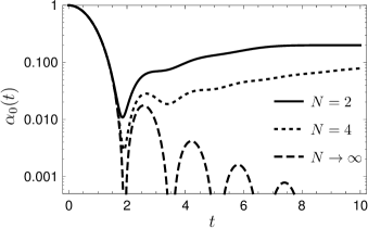
Figure 1: $\alpha_{0}(t)$ as a function of time for different dimensions $N$. Nonmonotonic behavior, causing non-Markovianity, is observed even in the limit of large dimensions, $N\to\infty$. Here, as well as in all subsequent figures, time is measured in dimensionless units, as explained in the main text below Eq. (8).

II.2 Non-Markovianity in the fully coupled system

Quantum non-Markovianity does not have a unique definition. Definitions include considering any deviation from the Lindblad equation as non-Markovian behavior Wolf et al. (2008), the backflow of information from the environment into the system Laine et al. (2010), and also the impossibility of defining an instantaneous quantum map for intermediate times Rivas et al. (2010). Accordingly, several measures have been proposed to quantify the degree of non-Markovianity, each with different properties and problems Breuer (2012); Ángel Rivas et al. (2014). However, for simple channels, like a depolarizing channel, as in our case, most definitions coincide as far as the distinction between Markovianity and non-Markovianity is concerned Žnidarič et al. (2011), even though the measures of the degree of non-Markovianity are usually not comparable. For the sake of definitiveness we shall use the measure proposed in Laine et al. (2010), although other measures could be easily incorporated in this framework. The measure is defined as the maximum of the integrated backflow of information measured in terms of increasing distinguishability, where the maximum is taken over all possible pairs of initial states. In the present case, where the quantum process is determined in terms of the function $\alpha(t)$, one gets Žnidarič et al. (2011)

$$\mathcal{M}=2\int_{\dot{\alpha}>0}^{\infty}\mathrm{d}t\;\dot{\alpha}(t)\;.$$ (12)

The measure will be greater than zero if and only if $\dot{\alpha}(t)>0$ for some time, i.e. if the Bloch sphere expands during a time interval. One of the results of Ref. Žnidarič et al. (2011) says that the system will generically display non-Markovianity, even in the limit of an infinite dimensional environment ($N\to\infty$); see Fig. 1. One may compare the present model to the case of an environment modeled by a collection of harmonic oscillators, characterized by a spectral density $J(w)$; see Breuer and Petruccione (2002), chap. 10. In those models this spectral density has a role similar to the level density in ours (however, see Stockburger and Grabert (2002); Alonso and de Vega (2007)), as it is the forms of those functions which determine the reduced dynamics and thereby the (non-)Markovianity. This similarity is surprising, since we are dealing with a very strong coupling limit, whereas the description based on the spectral density relies on a weak coupling approximation. In this respect, we also find it surprising that at strong but finite coupling, our model shows a transition to Markovian dynamics, independent of the level density. That case will be discussed in Sec. IV.

At finite $N$, the non-Markovianity has two contributions acting at different time scales. The first comes from the oscillations in the one-point function $b_{1}(t)$, which appear on a timescale independent of the dimension $N$ of the environment (the macroscopic timescale). The second contribution comes from a recovery of $\alpha(t)$ between the first zero of $J_{1}(2t)$ and the long-time limit

$$\lim_{t\to\infty}\alpha(t)=\frac{1}{2N+1}.$$ (13)

That occurs on the timescale of the Heisenberg time $\tau_{\text{H}}$ of the environment, which is proportional to $N$. In the semiclassical limit, $N\to\infty$, the Heisenberg time goes to infinity and the recovery goes to zero. As a consequence, $\lim_{N\to\infty}\mathcal{M}=0$, also.

III The weak-coupling limit

The behavior of $\alpha(t)$ in the weak-coupling limit can be deduced from previous results Pineda et al. (2007); Gorin et al. (2008), where the purity for a model equivalent to Eq. (2) was studied. In that limit, the relevant time scale is the Heisenberg time $\tau_{\text{H}}$ of the Hamiltonian $H_{\text{e}}$ of the environment. Since the focus was then put on the evolution of purity, $P=\mathop{\mathrm{tr}}\nolimits\rho^{2}$, we use the fact that purity can be expressed in terms of $\alpha(t)$ from Eq. (5) as follows:

$$P(t)=\mathop{\mathrm{tr}}\nolimits\left(\Lambda^{(t)}[\rho]\right)^{2}=\frac{1+\alpha(t)^{2}}{2}.$$ (14)

Switching from the parameter $s$, which scales the factorized term, to $\lambda$ scaling the coupling, we can write

$$H=H_{\text{e}}\otimes\openone+\lambda V.$$ (15)

$V$ is chosen from a GUE, but now with an $N$-independent scaling $\langle V_{ij}V_{kl}\rangle=\delta_{jk}\delta_{il}$. In order to map this Hamiltonian on Eq. (2), we would have to set $\lambda=1/(sN)$. In the case that $H_{\text{e}}$ and $V$ are both members of a GUE, it was found that, in the linear response approximation, the average purity is given by

$$P_{\text{LR}}(t)=1-\lambda^{2}g(t)$$ (16)

with

$$g(t)=2t\max\{t,\tau_{\text{H}}\}+\frac{2}{3\tau_{\text{H}}}(\min\{t,\tau_{\text{H}}\})^{3},$$ (17)

with $\tau_{\text{H}}$ being the Heisenberg time of $H_{\text{e}}$.

To go beyond the reach of linear response theory, we exponentiate the result, such that (i) the first two terms in a Taylor series coincide with the linear response result and (ii) the asymptotic value coincides with a theoretical expectation. Such a heuristic procedure, known as exponentiation, has lead to excellent results Gorin et al. (2006). In our case, the procedure leads to

$$P_{\text{ELR}}(t)=\frac{1}{2}+\frac{1}{2}\exp\left[\frac{1}{2}(P_{\text{LR}}(t)-1)\right].$$ (18)

Relying on self-averaging, which is often the case in these kind of systems Gorin et al. (2008), one can reconstruct $\alpha(t)$ for moderate values of the perturbation. Thereby, we obtain

$$\alpha(t)=\exp\left(-\frac{\lambda^{2}}{2}g(t)\right).$$ (19)

Notice that when the Heisenberg time becomes infinite, we obtain an exponential decay for $\alpha(t)$, a result also known as the Fermi golden rule. Notice also that $g(t)$ as defined in Eq. (17) is a monotonically increasing function, which implies that $\alpha(t)$ is monotonically decreasing. This means that the corresponding dynamics is Markovian, independent of the shape of the level density.

IV The strongly coupled system

So far we found that, for $N\to\infty$, the fully coupled system ($s=0$) shows non-Markovian dynamics, while at weak coupling, the system becomes Markovian. In this section, we consider the crossover region, when $s$ is small but finite. The linear response theory developed below is applicable as long as $s\lesssim 1$ when the free evolution term and the coupling in the Hamiltonian in Eq. (2) are of the same size. From a technical point of view, the calculation is much more demanding than usual, because the linear response expansion is around the fully coupled case.

IV.1 Linear response theory

We will calculate

$$\alpha(t)=\frac{1}{N}\left\langle\mathop{\mathrm{tr}}\nolimits\left[\sigma_{z}\otimes\openone_{\text{e}}\mathrm{e}^{-\imath Ht}\sigma_{z}\otimes\openone_{\text{e}}\mathrm{e}^{\imath Ht}\right]\right\rangle$$ (20)

with the ensemble defined in Eq. (2). To apply linear response theory for small $s$, we consider the unperturbed propagator to be $\mathrm{e}^{-\imath Vt}$, and the perturbation $sH_{\mathrm{e}}$. Hence, we have for the echo operator:

$$\mathrm{e}^{\imath Vt}\;\mathrm{e}^{-\imath Ht}\approx\openone-\imath s\int_{0}^{t}\mathrm{d}t^{\prime}\tilde{H}_{\mathrm{e}}(t^{\prime})\\ -s^{2}\int_{0}^{t}\mathrm{d}t^{\prime}\int_{0}^{t^{\prime}}\mathrm{d}t^{\prime\prime}\tilde{H}_{\mathrm{e}}(t^{\prime})\tilde{H}_{\mathrm{e}}(t^{\prime\prime}),$$ (21)

where $\tilde{X}(t)=\mathrm{e}^{\imath Vt}X\mathrm{e}^{-\imath Vt}$ denotes the interaction picture of operator $X$. After some calculations, detailed in Appendix B, we find that

$$\alpha(t)\approx\alpha_{0}(t)-s^{2}\alpha_{2}(t)$$ (22)

where

$$\alpha_{2}(t)=\frac{2}{N}{\rm Re}\int_{0}^{t}\mathrm{d}t^{\prime}\int_{0}^{t^{\prime}}\mathrm{d}t^{\prime\prime}\left(A^{(1)}-A^{(2)}\right)$$ (23)

and

$$A^{(1)} =\left\langle{\rm tr}\big{[}\mathrm{e}^{\imath Vt}\sigma_{z}\mathrm{e}^{-\imath V(t-t^{\prime})}H_{\mathrm{e}}\mathrm{e}^{-\imath V(t^{\prime}-t^{\prime\prime})}H_{\mathrm{e}}\mathrm{e}^{-\imath Vt^{\prime\prime}}\sigma_{z}\big{]}\right\rangle,$$ (24)

$$A^{(2)} =\left\langle{\rm tr}\big{[}\mathrm{e}^{\imath V(t-t^{\prime\prime})}\sigma_{z}\mathrm{e}^{-\imath V(t-t^{\prime})}H_{\mathrm{e}}\mathrm{e}^{-\imath Vt^{\prime}}\sigma_{z}\mathrm{e}^{\imath V\,t^{\prime\prime}}H_{\mathrm{e}}\big{]}\right\rangle.$$ (25)

IV.2 Averaging over the unitary group

We shall work in the eigenbasis of the environmental Hamiltonian, so that $H_{\mathrm{e}}=\mathop{\mathrm{diag}}\nolimits\varepsilon_{k}$. Let us call $O$ the matrix of eigenvectors of $V$ so that $\mathrm{e}^{\imath Vt}=O\mathrm{e}^{\imath\vec{v}t}O^{\dagger}$, with $\vec{v}$ being the eigenvalues of $V$. Since $V$ is taken from a GUE, $O$ must be an element of the unitary group $U(2N)$ equipped with the Haar measure. Eq. (24) may be rewritten as

$$\langle A^{(1)}\rangle=\Big{\langle}\mathrm{e}^{\imath t(v_{\alpha}-v_{\beta})+\imath t^{\prime}(v_{\beta}-v_{\gamma})+\imath t^{\prime\prime}(v_{\gamma}-v_{\delta})}\Big{\rangle}\langle\varepsilon_{k}\varepsilon_{j}\rangle(-)^{a+d}\\ \times\Big{\langle}O_{dl,\alpha}O_{ai,\alpha}^{*}O_{ai,\beta}O_{bj,\beta}^{*}O_{bj,\gamma}O_{ck,\gamma}^{*}O_{ck,\delta}O_{dl,\delta}^{*}\Big{\rangle}\,.$$ (26)

In this equation the Einstein summation convention is used. The indices $a$, $b$, $c$, and $d$ run through the basis states of the qubit; the indices $i$, $j$, $k$, and $l$ through those of the environment; and the greek indices through the $2N$ eigenstates of the coupling operator $V$. Equation (26) is composed of three independent parts: The first part contains time and the eigenvalues of the coupling. The second one, contains the eigenvalues of the environment Hamiltonian, and the third part contains the term $(-)^{a+d}$ and the eigenvectors of $V$. The term $A^{(2)}$ can be decomposed similarly. Notice that one can go from Eq. (24) to Eq. (25) performing the following substitutions:

$$\begin{array}[]{cccccc}A^{(1)}&\to&A^{(2)}&\qquad A^{(1)}&\to&A^{(2)}\\ t&\to&t^{\prime\prime}&\qquad\alpha&\to&\delta\\ t^{\prime}&\to&t&\qquad\beta&\to&\alpha\\ t^{\prime\prime}&\to&t^{\prime}&\qquad\gamma&\to&\beta\\ &&&\qquad\delta&\to&\gamma\end{array}\,.$$ (27)

Using these rules, one can write the analogous expression for $A^{(2)}$, starting from Eq. (26). As is well known Mello and Seligman (1980), averages over the unitary matrices with respect to the Haar measure are invariant under arbitrary permutations of columns and/or rows. Hence, the result of those averages only depends on the question of whether these indices coincide among each other or not. We may use this invariance property to get rid of the factor $(-)^{a+d}$ as follows: Assume $i\neq l$; then the row $ai$ is always different from $dl$ and the group average does not depend on $a$ and $d$, so the summation over $a$ and $d$ can be factored and yields $\sum_{a,d}(-)^{a+d}=0$. Therefore, we may restrict the summation to the case $i=l$.

The different terms in the summation in Eq. (26) can be grouped according to the degeneracy of the indices; the particular value of each index is unimportant. One can therefore divide the set of values for the four Greek indices into 15 different partitions, which will be enumerated as follows:

$$\begin{array}[]{ccl}1&:&\alpha=\beta=\gamma=\delta\\ \hline\cr 2&:&\alpha=\beta=\gamma\neq\delta\\ 3&:&\alpha=\beta=\delta\neq\gamma\\ 4&:&\alpha=\gamma=\delta\neq\beta\\ 5&:&\alpha\neq\beta=\gamma=\delta\\ \hline\cr 6&:&\alpha=\beta\neq\gamma=\delta\\ 7&:&\alpha=\gamma\neq\beta=\delta\\ 8&:&\alpha=\delta\neq\beta=\gamma\end{array}\;\qquad\begin{array}[]{ccl}9&:&\alpha=\beta\neq\gamma\neq\delta\\ 10&:&\alpha=\gamma\neq\beta\neq\delta\\ 11&:&\alpha=\delta\neq\beta\neq\gamma\\ 12&:&\alpha\neq\delta\neq\beta=\gamma\\ 13&:&\alpha\neq\gamma\neq\beta=\delta\\ 14&:&\alpha\neq\beta\neq\gamma=\delta\\ \hline\cr 15&:&\alpha\neq\beta\neq\gamma\neq\delta\end{array}\;.$$ (28)

For the latin index pairs we can proceed likewise. Due to the invariance properties of the averages of the monomials, based on the above labeling of the partitions, we can write

$$A^{(1)} =\sum_{I=1}^{15}\sum_{J=1}^{15}C_{I}M_{IJ}^{(1)}F_{J}^{(1)}=\bm{C}^{T}\bm{M}^{(1)}\bm{F}^{(1)},$$

$$A^{(2)} =\bm{C}^{T}\bm{M}^{(2)}\bm{F}^{(2)}.$$ (29)

Notice that we are using capital latin letters as indices for the different partitions. In this equation, $\bm{C}$ is a vector containing all $C_{I}$ cases, in which the terms $\langle\varepsilon_{j}\varepsilon_{k}\rangle$ and $(-)^{a+d}$ are taken into account; in the matrices $\bm{M}^{(1,2)}$, the group averages over the monomials of matrix elements of $O$ are arranged, and the time-dependent phases containing the eigenvalues of the coupling are are included in $\bm{F}^{(1,2)}$. The partitions, Eq. (28), with respect to row indices (latin index pairs) and column indices (greek indices) have different multiplicities, which are included in the vectors $\bm{C}$ and $\bm{F}^{(1,2)}$, respectively. The factors $C_{I}$ are the same for $A^{(1)}$ and $A^{(2)}$. We find that

$$C_{1} =-C_{2}=-C_{5}=-C_{6}=-C_{7}=2N,$$

$$C_{3} =C_{4}=-2(N-2),\,C_{8}=2N(2N-1)$$

$$C_{9} =4(N-1),C_{10}=-C_{12}=C_{13}=C_{14}=4(N-1)$$

$$C_{11} =-4(N-1)(N-2),C_{15}=4(N-1)(N-4).$$

The group averages appearing in the matrices $\bm{M}^{(1,2)}$ are calculated exactly for arbitrary $N$, based on recursion formulas developed in Gorin and López (2008), available as computer code in cod (2015). We report the results of the vectors $\bm{C}^{T}\bm{M}^{(1,2)}$:

$$\bm{C}^{T}\bm{M}^{(1)}=\frac{1}{N(2N+1)(2N+3)}\Big{(}N+4,\frac{N-1}{2N-1},\frac{2(N-1)(N+2)}{2N-1},\frac{N-1}{(2N-1)},\frac{2(N^{2}+3N+1)}{(2N-1)},-\frac{N-1}{N(2N-1)},$$

$$\frac{(N-1)(N+2)(2N+1)}{N(2N-1)},-\frac{N-1}{N(2N-1)},-\frac{N-1}{2N(2N-1)},-\frac{3N+2}{2N(2N-1)},-\frac{N-1}{2N(2N-1)},$$

$$-\frac{N-1}{2N(2N-1)},\frac{4N^{3}+6N^{2}-3N-2}{2N(2N-1)},-\frac{N-1}{2N(2N-1)},\frac{5}{2(2N-3)(2N-1)}\Big{)}$$ (30)

and

$$\bm{C}^{T}\bm{M}^{(2)}=\frac{1}{N(2N+1)(2N+3)}\Big{(}N+4,\frac{N-1}{2N-1},\frac{N-1}{2N-1},\frac{N-1}{2N-1},\frac{N-1}{2N-1},-\frac{N-1}{N(2N-1)},\frac{2(N-1)(N+1)}{N(2N-1)},$$

$$\frac{(N+1)(4N+1)}{N(2N-1)},\frac{2N^{2}+2N+1}{2N(2N-1)},\frac{(N-1)(N+1)}{N(2N-1)},\frac{2N^{2}+2N+1}{2N(2N-1)},\frac{2N^{2}+2N+1}{2N(2N-1)},\frac{(N-1)(N+1)}{N(2N-1)},$$

$$\frac{2N^{2}+2N+1}{2N(2N-1)},\frac{2(N-1)(N+1)}{(2N-3)(2N-1)}\Big{)}.$$ (31)

IV.3 Average over the eigenvalues of $V$

We now calculate the components $F^{(1,2)}_{I}$ of the time-dependent factors $\bm{F}^{(1,2)}$. As we are mainly interested in the case of large $N$, we shall ignore all spectral correlations, as these could only affect the dynamics of the qubit at times proportional to $N$, where $\alpha(t)$ already is of order of $1/N$. We have seen this explicitly in Sec. II.1, where we considered the case of full coupling, $s=0$. We expect that, for the perturbed case with finite $s$, the situation will be similar, and will be justified a posteriori with the numerical simulations. In other words, we assume that the eigenvalues of the coupling term $V$ have a semicircle spectral density, but are otherwise statistically independent. Note, however, that in principle, one could take into account correlations and describe the behavior up to times of the order of the Heisenberg time, if required.

$\nu$	$\left[{\bf C}^{T}{\bf M}^{(1)}\right]_{\nu}$	$F^{(1)}_{\nu}$	$\left[A^{(1)}\right]_{\nu}$	$\left[{\bf C}^{T}{\bf M}^{(2)}\right]_{\nu}$	$F^{(2)}_{\nu}$	$\left[A^{(2)}\right]_{\nu}$
1	-2	1	-1	-2	1	-1
2	-3	2	-1	-3	2	-1
3	-2	2	0	-3	2	-1
4	-3	2	-1	-3	2	-1
5	-2	2	0	-3	2	-1
6	-3	2	-1	-4	2	-2
7	-2	2	0	-3	2	-1
8	-4	2	-2	-3	2	-1
9	-4	3	-1	-3	3	0
10	-4	3	-1	-3	3	0
11	-4	3	-1	-3	3	0
12	-4	3	-1	-3	3	0
13	-2	3	1	-3	3	0
14	-4	3	-1	-3	3	0
15	-5	4	-1	-3	4	1

Table 1: (Color online) Order of magnitude of the 15 different terms [see Eq. (28)] contributing to Eq. (22). The leading terms are shaded (in green). Thus, for large $N$, it is enough to consider the 13th term of $A^{(1)}$ and the 15th term of $A^{(2)}$.

That said, all components $F^{(1,2)}_{I}$ will depend solely on the Fourier transform of the spectral density $b_{1}$. With the help of the auxiliary functions

$$\mathcal{F}(x) =\frac{(2N)!}{(2N-2)!}b_{1}^{2}(x),$$

$$\mathcal{G}(x,y,z) =\frac{(2N)!}{(2N-3)!}b_{1}(x)b_{1}(y)b_{1}(z),$$ (32)

$$\mathcal{H}(x,y,z) =\frac{(2N)!}{(2N-4)!}b_{1}(x)b_{1}(y-x)b_{1}(z-y)b_{1}(z).$$

we may write

$$\langle F_{1}^{(1)}\rangle =2N, \langle F_{9}^{(1)}\rangle =\mathcal{G}(t^{\prime},t^{\prime\prime}-t^{\prime},t^{\prime\prime}),$$

$$\langle F_{2}^{(1)}\rangle =\mathcal{F}(t^{\prime\prime}), \langle F_{10}^{(1)}\rangle =\mathcal{G}(t+t^{\prime\prime}-t^{\prime},t^{\prime}-t,t^{\prime\prime}),$$

$$\langle F_{3}^{(1)}\rangle =\mathcal{F}(t^{\prime}-t^{\prime\prime}), \langle F_{11}^{(1)}\rangle =\mathcal{G}(t-t^{\prime\prime},t^{\prime}-t,t^{\prime\prime}-t^{\prime}),$$

$$\langle F_{4}^{(1)}\rangle =\mathcal{F}(t-t^{\prime}), \langle F_{12}^{(1)}\rangle =\mathcal{G}(t,t^{\prime\prime}-t,t^{\prime\prime}),$$

$$\langle F_{5}^{(1)}\rangle =\mathcal{F}(t), \langle F_{13}^{(1)}\rangle =\mathcal{G}(t,-t+t^{\prime}-t^{\prime\prime},t^{\prime\prime}-t^{\prime}),$$

$$\langle F_{6}^{(1)}\rangle =\mathcal{F}(t^{\prime}), \langle F_{14}^{(1)}\rangle =\mathcal{G}(t,t^{\prime}-t,t^{\prime}),$$

$$\langle F_{7}^{(1)}\rangle =\mathcal{F}(t-t^{\prime}+t^{\prime\prime}), \langle F_{15}^{(1)}\rangle =\mathcal{H}(t,t^{\prime},t^{\prime\prime})\,.$$

$$\langle F_{8}^{(1)}\rangle =\mathcal{F}(t-t^{\prime\prime}),$$ (33)

Finally, using the mapping (27), we also obtain the components of $F^{(2)}$:

$$\langle F_{1}^{(2)}\rangle =2N, \langle F_{9}^{(2)}\rangle =\mathcal{G}(t^{\prime\prime},t^{\prime}-t^{\prime\prime},t^{\prime}),$$

$$\langle F_{2}^{(2)}\rangle =\mathcal{F}(t^{\prime\prime}), \langle F_{10}^{(2)}\rangle =\mathcal{G}(t^{\prime\prime},-t^{\prime\prime}+t-t^{\prime},t^{\prime}-t),$$

$$\langle F_{3}^{(2)}\rangle =\mathcal{F}(t^{\prime}), \langle F_{11}^{(2)}\rangle =\mathcal{G}(t,t^{\prime}-t,t^{\prime}),$$

$$\langle F_{4}^{(2)}\rangle =\mathcal{F}(t-t^{\prime}), \langle F_{12}^{(2)}\rangle =\mathcal{G}(t^{\prime\prime},t-t^{\prime\prime},t),$$

$$\langle F_{5}^{(2)}\rangle =\mathcal{F}(t^{\prime\prime}-t), \langle F_{13}^{(2)}\rangle =\mathcal{G}(t^{\prime\prime}+t^{\prime}-t,t-t^{\prime\prime},t^{\prime}),$$

$$\langle F_{6}^{(2)}\rangle =\mathcal{F}(t^{\prime\prime}-t^{\prime}), \langle F_{14}^{(2)}\rangle =\mathcal{G}(t^{\prime\prime}-t^{\prime},t-t^{\prime\prime},t^{\prime}-t),$$

$$\langle F_{7}^{(2)}\rangle =\mathcal{F}(t^{\prime\prime}-t+t^{\prime}), \langle F_{15}^{(2)}\rangle =\mathcal{H}(t^{\prime\prime},t,t^{\prime})\,.$$

$$\langle F_{8}^{(2)}\rangle =\mathcal{F}(t),$$ (34)

Equations (22), (23), and (29), together with Eqs. (30) to (34), provide the final, general result. It is valid, either in the absence of spectral correlations in $H_{\text{e}}$, or for large $N$ at times sufficiently small compared to the Heisenberg time. In our case, $b_{1}(t)$ is given in Eq. (11), which corresponds to a semicircle level density. However, other cases with different level densities could be considered, also. Our general result still requires the evaluation of the double time integral in Eq. (23). Typically, one would have to do this evaluation numerically.

IV.4 The solution for large dimensions and times

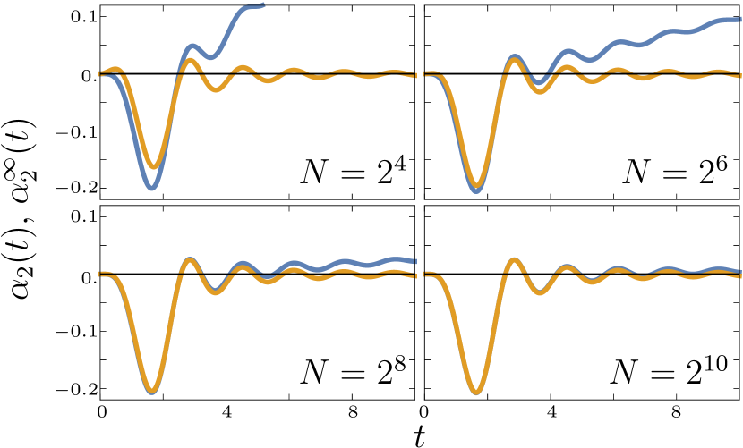
Figure 2: (Color online) Exact value of the integral $\alpha_{2}(t)$ in Eq. (23), with all terms (yellow curves) and only taking into account the leading terms in $N$ (blue curves); that is, the value of $\alpha_{2}^{\infty}(t)$, for several values of the dimension $N$.

It is possible to simplify the general expressions, discussed above, considering explicitly the limit of large $N$. Table 1 indicates the leading order in $N^{-1}$ of all relevant terms, in Eqs. (30), (31), and (32). By proper selection of the highest order terms, we obtain for $\alpha_{2}^{\infty}(t)=\lim_{N\to\infty}\alpha_{2}(t)$ the following

$$\alpha_{2}^{\infty}(t)=2\int_{0}^{t}\mathrm{d}t^{\prime}\int_{0}^{t^{\prime}}\mathrm{d}t^{\prime\prime}\bigg{(}b_{1}(t)b_{1}(t^{\prime}-t-t^{\prime\prime})b_{1}(t^{\prime\prime}-t^{\prime})\\ -b_{1}(t^{\prime\prime})b_{1}(t-t^{\prime\prime})b_{1}(t^{\prime}-t)b_{1}(t^{\prime})\bigg{)}.$$ (35)

We have tested the reach of this limit in fig. 2, where we can see that already for $N=2^{10}$ there is almost no visible difference, for the times reported, between the full expression and the large-environment limit. Although this expression means a considerable simplification for the $b_{1}$ from a semicircle level density, we were still not able to solve the time integrals in closed form. We found only one case where that is possible. This case, where the level density is a Gaussian function, is treated in Appendix D.

IV.5 The solution for large times

Linear response theory is valid whenever the corrections in the echo operator, Eq. (21), with respect to the identity are small; that is, whenever $|\mathrm{e}^{\imath Vt}\mathrm{e}^{-\imath Ht}-\openone|\ll 1$ (here, $|\,\cdot\,|$ denotes the operator norm). This implies that the eigenvalues of the echo operator must remain close to 1. Departure from that happens for any value of the perturbation $s$, for sufficiently long times. However, the smaller the $s$, the larger the time of the validity of the linear response approximation.

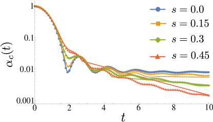
Figure 3: (Color online) Comparison of the linear response theory, with an exponential tail, and the numerical simulation, with $N=64$, for several perturbations.

The extension of linear response formulas in this context is often done using exponentiation, as in Sec. III. However, in the present case such attempts have been unsuccessful Garrido (2015). As an alternative, we have opted to combine the two linear response theories, namely the ones discussed in Sec. III and Sec. IV.1. We shall use the linear response formula Eq. (22) until the time in which the largest (in absolute value) eigenphase reaches $\pm\pi$. Afterwards, an exponential decay is fitted.

V The transition from non-Markovian to Markovian behavior

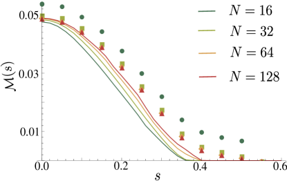
Figure 4: (Color online) Measure of non-Markovianity for a random Hamiltonian of the form Eq. (2). Here, both matrices $V$ and $H_{\text{e}}$ are taken from the GUE, and the dimension of the environment $N$ is varied. Symbols indicate calculations done with the linear response theory, extended with an exponential decay, while continuous lines are obtained numerically. One can see that, at a critical intensity of the coupling $s\approx 0.4$, the system switches from non-Markovian to Markovian. It should also be noted that, as the dimension increases the approximations are more accurate.

As the coupling of the system diminishes (that is, when $s$ increases), one should fall back to the Markovian case in the large-dimension limit Breuer (2012); Gorin et al. (2008); cf. also Sec. III. This is indeed observed in fig. 3, where the curves for $\alpha(t)$ become monotonic as $s$ increases. Thus, we would like to know whether there is a particular value for $s$ beyond which the dynamics is Markovian. This question is answered in fig. 4, where the measure for non-Markovianity, from Eq. (12) is plotted as a function of the coupling $s$. The points mark the numerical results for $\mathcal{M}$ where the integration in Eq. (12) has been restricted to the interval $t\in[0,10]$. While this introduces an error at small dimensions, this error vanishes at large $N$. The solid lines mark the same quantity, but calculated from the composite linear response results shown in fig. 3. One can observe that there is a seemingly sharp transition in the large-dimension limit, which is not observed for smaller dimensions due to the two-point correlations that cause an increase in the function $\alpha$, and are not taken into account in the linear response results.

It is remarkable that a critical value of the coupling is needed to go from one regime into the other. It must be noticed, however, that in our calculation we are using an ensemble of Hamiltonians to describe the environment and the coupling to it. In a real experiment this would correspond to measurements which require many repetitions of the quantum process, during which the dynamics in the environment changes, e.g., due to fluctuating classical fields. A particular member of the ensemble will exhibit oscillations that will result in non-Markovianity. However, one should distinguish oscillations due to the particularities of the system, from generic oscillations due to general features of the whole ensemble.

For completeness, we have also studied the case in which the qubit has an internal Hamiltonian, where Eq. (2) is substituted by

$$H=\omega\sigma_{z}+s\openone_{2}\otimes H_{\text{e}}+V.$$ (36)

This Hamiltonian is no longer invariant under unitary transformations in the central system, and hence Eq. (5) is no longer valid. Instead, the new quantum channel will be a combination of a dephasing and a depolarizing channel. The only energy scale retained in the limit of large dimensions is the spectral span of the coupling Hamiltonian $V$ [the level density has the shape of a semi-circle in the interval $(-1,1)$]. Therefore, one may expect that the effect of the additional term depends on the size of $\omega$ as compared to the spectral span. Hence, for $\omega\ll 1$ the effect should be negligible, we do expect differences for $\omega\gtrsim 1$. In Fig. 5, we present simulations for different values of $\omega$. The figure shows our measure for non-Markovianity as a function of $s$, just as in Fig. 4. We can observe, that increasing $\omega$ leads to larger values for the measure, but that the transition from non-Markovian to Markovian behavior is essentially unchanged.

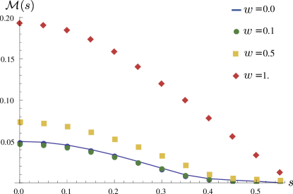
Figure 5: The effect of an internal Hamiltonian in the central system, as in Eq. 36, is studied. The level splitting, $\omega$, amplifies the non-Markovian effects, but apparently conserves the transition from non-Markovian to Markovian behavior, which occurs at approximately the same critical value for $s$.

VI Conclusions

We considered a quantum two-level system coupled to a generic environment modeled by random matrix theory. We obtained analytical expressions for the reduced dynamics using linear response approximations, both around the weak and strong coupling limits. For the weak-coupling limit, an explicit expression is obtained. The corresponding expression involves a double time-integral of one- and two-point functions of the coupling in the general case, a of one-point functions in the large dimension limit. In the limit $N\to\infty$, the result becomes much simpler [see Eq. (35)]: only two terms survive, which contain one-point functions. Nevertheless, the double time-integral still has to be evaluated numerically.

We then studied the degree of non-Markovianity in the system, using the measure proposed in Laine et al. (2010), based on distinguishability. We show that the degree of non-Markovianity of the $s=0$ case (infinite coupling) considered in Ref. Žnidarič et al. (2011) diminishes as the coupling term becomes less important, and that in the large-$N$ limit it vanishes at a point where the free and coupling terms of the Hamiltonian are of equal size.

Acknowledgements– Support by projects CONACyT 153190, CONACyT 129309 and UNAM-PAPIIT IN111015 are acknowledged.

Appendix A Details for the fully coupled case, in the GUE case

The spectral correlations for the GUE are expressed in terms of the functions

$$\phi_{j}(E)=\frac{\mathrm{e}^{-2NE^{2}/4}}{\sqrt{2^{j}j!\sqrt{2\pi/(2N)}}}\mathcal{H}_{j}(E\sqrt{N}),$$

where $\mathcal{H}_{j}$ are Hermite polynomials Mehta (1991).

We fix the normalization so the average of the square of the diagonal elements in the matrices is $1/N$. Then, the spectral density for finite dimensions is

$$R_{1}(E)=\sum_{j=0}^{2N-1}\phi_{j}(E)^{2}$$ (37)

and the cluster function, containing the correlations between levels, is

$$T_{2}(E_{1},E_{2})=\left(\sum_{j=0}^{2N-1}\phi_{j}(E_{1})\phi_{j}(E_{2})\right)^{2}\,.$$ (38)

If we define

$$b_{1}(t)=\frac{1}{2N}\int dE\mathrm{e}^{-\imath Et}R_{1}(E)$$ (39)

and

$$b_{2}(t)=\frac{1}{2N}\int dE_{1}dE_{2}\mathrm{e}^{-\imath(E_{1}-E_{2})t}T_{2}(E_{1},E_{2})$$ (40)

we have, for this case,

$$\langle\alpha_{0}(t)_{\mathrm{GUE}}\rangle=\frac{4N^{2}b_{1}^{2}(t)+4N(1-b_{2}(t))-1}{4N^{2}-1}\,,$$ (41)

since

$$N^{2}\langle f(t)|^{2}\rangle=N+\\ \int\mathrm{d}E_{1}\mathrm{d}E_{2}\mathrm{e}^{-\mathrm{i}(E_{1}-E_{2})t}[R_{1}(E_{1})R_{1}(E_{2})-T_{2}(E_{1},E_{2})].$$ (42)

In the large dimension limit, we have

$$b_{1}(t)=\frac{J_{1}(2t)}{t}\,$$ (43)

and thus

$$\lim\limits_{N\rightarrow\infty}\langle\alpha_{0}(t)\rangle_{\mathrm{GUE}}=\left[\frac{J_{1}(2\,t)}{t}\right]^{2}.$$ (44)

Appendix B Details for the linear response theory

Now, we write $\alpha(t)$ in terms of the echo operator as follows:

$$\alpha(t)={\rm tr}\Big{[}\,\sigma_{z}\otimes\openone\;\mathrm{e}^{-\imath V\,t}\;M\;\sigma_{z}\otimes\openone\;M^{\dagger}\;\mathrm{e}^{\imath V\,t}\,\Big{]}\;.$$ (45)

Using Born approximation Eq. (21), we obtain

$$\alpha(t) ={\rm tr}\big{[}\,\tilde{\sigma}_{z}(t)\;M\;\sigma_{z}\otimes\openone\;M^{\dagger}\,\big{]}$$

$$\approx\alpha_{0}(t)-s^{2}\int_{0}^{t}\mathrm{d}t^{\prime}\int_{0}^{t^{\prime}}\mathrm{d}t^{\prime\prime}{\rm tr}A(t^{\prime\prime},t^{\prime},t),$$

where

$$\alpha_{0}(t)={\rm tr}\left[\tilde{\sigma}_{z}(t)\sigma_{z}\otimes\openone\right]$$ (46)

represent the exact known solution for $s=0$, and

$$A(t^{\prime\prime},t^{\prime},t) =\tilde{\sigma}_{z}(t)\tilde{H}_{\mathrm{e}}(t^{\prime})\tilde{H}_{\mathrm{e}}(t^{\prime\prime})\sigma_{z}-\tilde{\sigma}_{z}(t)\tilde{H}_{\mathrm{e}}(t^{\prime})\sigma_{z}\tilde{H}_{\mathrm{e}}(t^{\prime\prime})$$

$$\,+\sigma_{z}\tilde{H}_{\mathrm{e}}(t^{\prime\prime})\tilde{H}_{\mathrm{e}}(t^{\prime})\tilde{\sigma}_{z}(t)-\tilde{\sigma}_{z}(t)\tilde{H}_{\mathrm{e}}(t^{\prime\prime})\sigma_{z}\tilde{H}_{\mathrm{e}}(t^{\prime}).$$

Due to the fact that the matrices $\tilde{H}_{\mathrm{e}}$, $\tilde{\sigma}_{z}$ and $\sigma_{z}\otimes\openone$ are Hermitian, we obtain the useful identities

$${\rm tr}\big{[}\tilde{\sigma}_{z}(t)\tilde{H}_{\mathrm{e}}(t^{\prime})\tilde{H}_{\mathrm{e}}(t^{\prime\prime})\sigma_{z}\big{]}^{*}={\rm tr}\big{[}\sigma_{z}\tilde{H}_{\mathrm{e}}(t^{\prime\prime})\tilde{H}_{\mathrm{e}}(t^{\prime})\tilde{\sigma}_{z}(t)],$$

and

$${\rm tr}\big{[}\tilde{\sigma}_{z}(t)\tilde{H}_{\mathrm{e}}(t^{\prime})\sigma_{z}\tilde{H}_{\mathrm{e}}(t^{\prime\prime})\big{]}^{*} ={\rm tr}\big{[}\tilde{H}_{\mathrm{e}}(t^{\prime\prime})\sigma_{z}\tilde{H}_{\mathrm{e}}(t^{\prime})\tilde{\sigma}_{z}(t)\big{]}$$

$$={\rm tr}\big{[}\tilde{\sigma}_{z}(t)\tilde{H}_{\mathrm{e}}(t^{\prime\prime})\sigma_{z}\tilde{H}_{\mathrm{e}}(t^{\prime})\big{]}.$$

This implies that the trace of $A(t^{\prime\prime},t^{\prime},t)$ can be written as twice the real part of the trace of $A_{\rm c}(t^{\prime\prime},t^{\prime},t)$, where the latter quantity only contains the two terms on the left-hand side of the above equation. We may thus write for $\alpha(t)$ in the linear response approximation:

$$\alpha(t)\approx\alpha_{0}(t)-2\,s^{2}\;{\rm Re}\int_{0}^{t}\mathrm{d}t^{\prime}\int_{0}^{t^{\prime}}\mathrm{d}t^{\prime\prime}\;{\rm tr}\big{[}\,A_{\rm c}(t^{\prime\prime},t^{\prime},t)\,\big{]}\;,$$

where

$$A_{\rm c}(t^{\prime\prime},t^{\prime},t)=\tilde{\sigma}_{z}(t)\tilde{H}_{\mathrm{e}}(t^{\prime})\tilde{H}_{\mathrm{e}}(t^{\prime\prime})\sigma_{z}-\tilde{\sigma}_{z}(t)\tilde{H}_{\mathrm{e}}(t^{\prime})\sigma_{z}\tilde{H}_{\mathrm{e}}(t^{\prime\prime}).$$

Now we split $A_{\rm c}$ in its two parts,

$${\rm tr}A_{\rm c}(t^{\prime\prime},t^{\prime},t)=A^{(1)}-A^{(2)},$$

insert identity operators $\mathrm{e}^{-\imath V\,t}\mathrm{e}^{\imath V\,t}$ wherever necessary, and use the cyclical property of the trace, to rewrite more conveniently the term under the integral.

Appendix C Normalization of the ensembles considered

In Sec. IV.1, we are free to consider any normalization condition.

We conveniently assume that, with respect to an arbitrary basis, the matrix elements of both $V$ and $H_{\mathrm{e}}$ have a variance equal to their inverse dimension. Let $H$ be either $V$ or $H_{\mathrm{e}}$, so the normalization condition reads

$$\langle H_{ij}\,H_{kl}\rangle=\frac{\delta_{jk}\delta_{li}}{N}\;.$$ (47)

That implies for the average of the trace of $H^{2}$ and for the square of the trace of $H$

$${\rm tr}(H^{2})=\sum_{jk}\langle H_{jk}H_{kj}\rangle=\frac{N^{2}}{N}=N,$$ (48)

$$\big{[}\,{\rm tr}(H)\,\big{]}^{2}=\sum_{jk}\langle H_{jj}H_{kk}\rangle=\sum_{j}\langle H_{jj}^{2}\rangle=1.$$ (49)

In turn, this means that the eigenvalues $\varepsilon_{j}$ of $H_{\mathrm{e}}$ lie essentially in the interval $(-2,2)$, and have a semi-circle distribution, for large $N$. In addition, since $\sum_{j}\langle\varepsilon_{j}^{2}\rangle=N$,

$$\langle\varepsilon_{j}^{2}\rangle=1,$$ (50)

and, since $\sum_{jk}\langle\varepsilon_{j}\varepsilon_{k}\rangle=N+N(N-1)\langle\varepsilon_{j}\varepsilon_{k}\rangle=1$,

$$\langle\varepsilon_{j}\varepsilon_{k}\rangle_{j\neq k}=-\frac{1}{N}.$$ (51)

Appendix D The Gaussian PUE

Initial calculations were done in a Poissonian ensemble with Gaussian level density. This could correspond to spin models. Even though non-Markovian effects are not visible here (the Fourier transform of a Gaussian, is another Gaussian), some results are easier to obtain, and provide a guide to the more complicated calculations in the GUE case. We present some details here, which might also provide a guide for the calculations using other spectral densities.

We now assume that the coupling $V$ is taken from the GPUE (Gaussian PUE). This means that $V$ is chosen as

$$V_{\rm GPUE}=UDU^{\dagger}\,,$$ (52)

with $U$ chosen from the unitary group with the Haar measure, and $D$ is a diagonal matrix with Gaussian independent numbers with $\sigma=1$. This means that the variables $v_{\mu}$ in Eq. (26) are, again, independent Gaussian variables with mean zero and unit standard deviation.

The subsequent calculation runs in identical way as shown in Sec. IV, except that in Eq. (43), we have

$$b_{1}(t)=\mathrm{e}^{-\frac{t^{2}}{2}},$$ (53)

and one has to propagate this difference through Eq. (32). In this case, some of the integrals involved in the terms $F^{(i)}_{\nu}$ can be performed, though not all.

In this case, the compact expression for the large dimension limit,

$$\alpha_{2}^{\infty}(t)\approx\sqrt{\pi}t\mathrm{e}^{-\frac{3t^{2}}{4}}\mathrm{Erf}\left(\frac{t}{2}\right)\,-\,\pi\mathrm{e}^{-\frac{t^{2}}{2}}\mathrm{Erf}\left(\frac{t}{2}\right)^{2},$$ (54)

is obtained.

References

• Žnidarič et al. (2011) M. Žnidarič, C. Pineda, and I. García-Mata, Phys. Rev. Lett. 107, 080404 (2011).
• Gorin and Seligman (2002) T. Gorin and T. H. Seligman, J. Opt. B: Quantum Semiclass. Opt. 4, S386 (2002), topical issue: Mysteries and Paradoxes in Quantum Mechanics IV Quantum interference phenomena (Workshop held at Gargano, Italy, August 2001).
• Gorin and Seligman (2003) T. Gorin and T. H. Seligman, Phys. Lett. A 309, 61 (2003).
• Guhr et al. (1998) T. Guhr, A. Müller-Groeling, and H. A. Weidenmüller, Phys. Rep. 299, 189 (1998).
• Berry and Tabor (1977) M. V. Berry and M. Tabor, Proc. R. Soc. Lond. A 356, 375 (1977).
• Casati et al. (1980) G. Casati, F. Valz-Gris, and I. Guarneri, Lett. Nuovo Cimento 28, 279 (1980).
• Bohigas et al. (1984) O. Bohigas, M. J. Giannoni, and C. Schmit, Phys. Rev. Lett. 52, 1 (1984).
• Blümel and Smilansky (1988) R. Blümel and U. Smilansky, Phys. Rev. Lett. 60, 477 (1988).
• Lutz and Weidenmüller (1999) E. Lutz and H. A. Weidenmüller, Physica A 267, 354 (1999).
• Gorin et al. (2008) T. Gorin, C. Pineda, H. Kohler, and T. H. Seligman, New J. Physics 10, 115016 (2008).
• Prosen et al. (2003) T. Prosen, T. H. Seligman, and M. Žnidarič, Prog. Theor. Phys. Supp. 150, 200 (2003), preprint only.
• Gorin et al. (2006) T. Gorin, T. Prosen, T. H. Seligman, and M. Znidaric, Phys. Rep. 435, 33 (2006).
• Mello and Seligman (1980) P. Mello and T. Seligman, Nucl. Phys. A 344, 489 (1980).
• Gorin and López (2008) T. Gorin and G. V. López, Journal of Mathematical Physics 49, 013503 (2008), URL http://quantum.cucei.udg.mx/~tgorin/paper/GL08JMP.pdf.
• Pineda et al. (2007) C. Pineda, T. Gorin, and T. H. Seligman, New Journal of Physics 9, 106:1 (2007), URL http://stacks.iop.org/1367-2630/9/106.
• Gorin et al. (2008) T. Gorin, C. Pineda, H. Kohler, and T. H. Seligman, New J. Phys. 10, 115016 (2008), eprint 0807.4913.
• Collins (2003) B. Collins, Int. Math. Res. Not. pp. 953–982 (2003), cited By 68, URL http://www.scopus.com/inward/record.url?eid=2-s2.0-0038239559&partnerID=40&md5=57de08b7c0e64d912a71f464b2d10d6c.
• Mehta (1991) M. L. Mehta, Random Matrices (Academic Press, San Diego, California, 1991), 2nd ed.
• Wolf et al. (2008) M. M. Wolf, J. Eisert, T. S. Cubitt, and J. I. Cirac, Phys. Rev. Lett. 101, 150402 (2008).
• Laine et al. (2010) E.-M. Laine, J. Piilo, and H.-P. Breuer, Phys. Rev. A 81, 062115 (2010).
• Rivas et al. (2010) Á. Rivas, S. Huelga, and M. Plenio, Phys. Rev. Lett. 105, 050403 (2010).
• Breuer (2012) H.-P. Breuer, J. Phys. B 45, 154001 (2012), URL http://stacks.iop.org/0953-4075/45/i=15/a=154001.
• Ángel Rivas et al. (2014) Ángel Rivas, S. F. Huelga, and M. B. Plenio, Rep. Prog. Phys. 77, 094001 (2014), URL http://stacks.iop.org/0034-4885/77/i=9/a=094001.
• Breuer and Petruccione (2002) H.-P. Breuer and F. Petruccione, The Theory of open quantum systems (Oxford University Press, 2002).
• Stockburger and Grabert (2002) J. T. Stockburger and H. Grabert, Phys. Rev. Lett. 88, 170407 (2002), URL http://link.aps.org/doi/10.1103/PhysRevLett.88.170407.
• Alonso and de Vega (2007) D. Alonso and I. de Vega, Phys. Rev. A 75, 052108 (2007), URL http://link.aps.org/doi/10.1103/PhysRevA.75.052108.
• cod (2015) libs, https://github.com/carlospgmat03/libs (2015).
• Garrido (2015) N. Garrido, Master’s thesis, Universidad Nacional Autónoma de México (2015).