Weak convergence of renewal shot noise processes in the case of slowly varying normalization

Abstract

We investigate weak convergence of finite-dimensional distributions of a renewal shot noise process $(Y(t))_{t\geq 0}$ with deterministic response function $h$ and the shots occurring at the times $0=S_{0}<S_{1}<S_{2}<\ldots$, where $(S_{n})$ is a random walk with i.i.d. jumps. There has been an outbreak of recent activity around this topic. We are interested in one out of few cases which remained open: $h$ is regularly varying at $\infty$ of index $-1/2$ and the integral of $h^{2}$ is infinite. Assuming that $S_{1}$ has a moment of order $r>2$ we use a strong approximation argument to show that the random fluctuations of $Y(s)$ occur on the scale $s=t+g(t,u)$ for $u\in[0,1]$, as $t\to\infty$, and, on the level of finite-dimensional distributions, are well approximated by the sum of a Brownian motion and a Gaussian process with independent values (the two processes being independent). The scaling function $g$ above depends on the slowly varying factor of $h$. If, for instance, $\lim_{t\to\infty}t^{1/2}h(t)\in(0,\infty)$, then $g(t,u)=t^{u}$.

2010 Mathematics Subject Classification: 60F05, 60K05

Keywords: Gaussian process with independent values $\cdot$ renewal shot noise process $\cdot$ weak convergence of finite-dimensional distributions

1 Introduction

Let $(\xi_{k})_{k\in\operatorname{\mathbb{N}}}$ be independent copies of a positive random variable $\xi$. Define a zero-delayed standard random walk $(S_{n})_{n\in\operatorname{\mathbb{N}}_{0}}$, where $\operatorname{\mathbb{N}}_{0}:=\operatorname{\mathbb{N}}\cup\{0\}$, by

$$S_{0}:=0,\quad S_{n}:=\xi_{1}+\ldots+\xi_{n},\quad n\in\operatorname{\mathbb{N}}.$$

For a locally bounded, measurable function $h:\operatorname{\mathbb{R}}^{+}\to\operatorname{\mathbb{R}}$, where $\operatorname{\mathbb{R}}^{+}:=[0,\infty)$, put $Y(t):=\sum_{k\geq 0}h(t-S_{k})\operatorname{\mathbbm{1}}_{\{S_{k}\leq t\}}$, $t\geq 0$. The process $Y:=(Y(t))_{t\geq 0}$ is called renewal shot noise process.

The renewal shot noise processes and their natural generalizations called random processes with immigration arise in most of natural sciences as well as diverse areas of applied probability. See [9] for a list of possible applications and the definition of the latter processes. A nice survey of earlier relevant literature can be found in [12].

Continuing the line of research initiated in [7, 8, 9, 10] we investigate weak convergence of the renewal shot noise processes. Here is a brief survey of the previously known results concerning weak convergence of finite-dimensional distributions which hold under the assumption that $\sigma^{2}:=\operatorname{\mathrm{Var}}\,\xi<\infty$. As for the case of infinite variance we refer the reader to the cited papers.

If the law of $\xi$ is nonarithmetic and $h:\operatorname{\mathbb{R}}^{+}\to\operatorname{\mathbb{R}}$ is a càdlàg function such that $|h(t)|\wedge 1$ is directly Riemann integrable on $\operatorname{\mathbb{R}}^{+}$ (we write $x\wedge y$ for $\min(x,y)$; the definition of the direct Riemann integrability can be found in Section 2), then the finite-dimensional distributions of $(Y(t+u))_{u\in\operatorname{\mathbb{R}}}$ converge weakly, as $t\to\infty$, to those of a stationary shot noise process. This is a consequence of Theorem 2.2 in [10]. Weak convergence of one-dimensional distributions has earlier been obtained in Theorem 2.1 in [8].

If the law of $\xi$ is nonarithmetic and $h:\operatorname{\mathbb{R}}^{+}\to\operatorname{\mathbb{R}}$ is a locally bounded, a.e. continuous, eventually nonincreasing and non-integrable function with $\int_{0}^{\infty}h^{2}(y){\rm d}y<\infty$, then $Y(t)-\mu^{-1}\int_{0}^{t}h(y){\rm d}y$ converges in distribution, as $t\to\infty$ (see Theorem 2.4 (C1) in [8]). Here and hereafter $\mu:=\operatorname{\mathbb{E}}\xi$. We believe that the finite-dimensional distributions of $(Y(t+u)-\mu^{-1}\int_{0}^{t+u}h(y){\rm d}y)_{u\in\operatorname{\mathbb{R}}}$ converge weakly, but this has never been proved.

Let $h:\operatorname{\mathbb{R}}^{+}\to\operatorname{\mathbb{R}}$ be locally bounded, measurable, eventually monotone and

$$h(t)\sim t^{\beta}\ell(t),\quad t\to\infty$$ (1.1)

for some $\beta>-1/2$ and some $\ell$ slowly varying at $\infty$. Then

$$\bigg{(}{Y(ut)-\mu^{-1}\int_{0}^{ut}h(y){\rm d}y\over\sqrt{\sigma^{2}\mu^{-3}t}h(t)}\bigg{)}_{u\geq 0}~{}\stackrel{{\scriptstyle\mathrm{f.d.}}}{{\to}}~{}\bigg{(}\int_{[0,\,u]}(u-y)^{\beta}{\rm d}B(y)\bigg{)}_{u\geq 0},\quad t\to\infty,$$ (1.2)

where $\stackrel{{\scriptstyle\mathrm{f.d.}}}{{\to}}$ denotes weak convergence of finite-dimensional distributions, $(B(u))_{u\geq 0}$ is a Brownian motion. This follows from Theorem 2.7 in [8] in the case when $h$ is eventually nonincreasing and from [7] in the case when $h$ is eventually nondecreasing.

In this paper we treat the borderline situation when $\beta$ in (1.1) equals $1/2$ yet the function $h^{2}$ is nonintegrable. This case bears some similarity with the case $\beta>-1/2$ (normalization is needed; the limit is Gaussian) and is very different from the case when $h^{2}$ is integrable. The principal new feature of the present case is necessity of sublinear time scaling as opposed to the time scalings $t+u$ and $ut$ used for the other regimes.

As might be expected of a transitional regime there are additional technical complications. In particular, the techniques (tools related to stationarity; the continuous mapping theorem along with the functional limit theorem for the first-passage time process of $(S_{n})$) used for the other regimes cannot be exploited here. Our main technical tool is a strong approximation theorem.

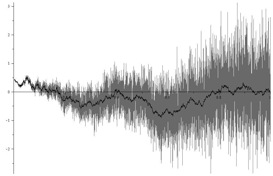
Figure 1: Grey graph: The limit process $X$. Black graph: The Brownian motion in reversed time $B(1-u)$.

Now we introduce a limit process $X:=(X(u))_{u\in[0,1]}$ appearing in Theorem 1.1 which is our main result. Let $B:=(B(u))_{u\in[0,1]}$ denote a Brownian motion independent of $D:=(D(u))_{u\in[0,1]}$, a centered Gaussian process with independent values which satisfies $\operatorname{\mathbb{E}}D^{2}(u)=u$. Then we set

$$X(u)=B(1-u)+D(u),\quad u\in[0,1].$$

In different contexts such a process has arisen in recent papers [3, 4]. The presence of $D$ makes the paths of $X$ highly irregular; see Figure 1. In particular, no version of $X$ lives in the Skorokhod space of right-continuous functions with finite limits from the left. The covariance structure of $X$ is very similar to that of $B$: for any $u,v\in[0,1]$

$${\rm cov}(X(u),X(v))=\begin{cases}(1-u)\wedge(1-v),&\text{if}\ u\neq v,\\ 1,&\text{if}\ u=v,\end{cases}$$

whereas ${\rm cov}(B(1-u),B(1-v))=(1-u)\wedge(1-v)$. Among others, this shows that neither $X$, nor $X(1-\cdot)$ is a self-similar process.

Theorem 1.1.

Suppose that $\operatorname{\mathbb{E}}\xi^{r}<\infty$ for some $r>2$ and that $h:\operatorname{\mathbb{R}}^{+}\to\operatorname{\mathbb{R}}$ is a right-continuous, locally bounded and eventually nonincreasing function. If

$$h(t)~{}\sim~{}t^{-1/2}\ell(t),\quad t\to\infty$$ (1.3)

for some $\ell$ slowly varying at $\infty$ such that $\int_{0}^{\infty}h^{2}(y){\rm d}y=\infty$, then, as $t\to\infty$,

$$\bigg{(}{Y(t+g(t,u))-\mu^{-1}\int_{0}^{t+g(t,u)}h(y){\rm d}y\over\sqrt{\sigma^{2}\mu^{-3}\int_{0}^{t}h^{2}(y){\rm d}y}}\bigg{)}_{u\in[0,1]}~{}\stackrel{{\scriptstyle\mathrm{f.d.}}}{{\to}}~{}(X(u))_{u\in[0,1]},$$

where $\sigma^{2}=\operatorname{\mathrm{Var}}\,\xi$, $\mu=\operatorname{\mathbb{E}}\xi$, and $g:\operatorname{\mathbb{R}}^{+}\times[0,1]\to\operatorname{\mathbb{R}}^{+}$ is any nondecreasing in the second coordinate function that satisfies

$$\lim_{t\to\infty}{\int_{0}^{g(t,u)}h^{2}(y){\rm d}y\over\int_{0}^{t}h^{2}(y){\rm d}y}=u$$ (1.4)

for each $u\in[0,1]$.

Remark 1.2.

To facilitate comparison with (1.2), observe that, under (1.1) with $\beta>-1/2$,

$$\sqrt{\int_{0}^{t}h^{2}(y){\rm d}y}~{}\sim~{}(2\beta+1)^{-1/2}\sqrt{t}h(t),\quad t\to\infty,$$

see Lemma 2.3(a), and therefore the normalization in (1.2) can be replaced (up to a multiplicative constant) by $(\int_{0}^{t}h^{2}(y){\rm d}y)^{1/2}$.

Remark 1.3.

Set $m(t):=\int_{0}^{t}h^{2}(y){\rm d}y$, $t>0$ and observe that, under (1.3), $m$ is a slowly varying function (see Lemma 2.3(b)) diverging to $+\infty$. Since $m$ is nondecreasing and continuous, the generalized inverse function $m^{\leftarrow}$ is increasing. Putting $g(t,u)=m^{\leftarrow}(um(t))$ gives us a nondecreasing in $u$ function that satisfies (1.4).

Remark 1.4.

Here we point out three types of possible time scalings which correspond to ’moderate’, ’slow’ and ’fast’ slowly varying $\ell$ in (1.3).

’Moderate’ $\ell$. If

$$\ell(t)=(\log t)^{(\rho-1)/2}L(\log t)$$ (1.5)

for some $\rho>0$ and some $L$ slowly varying at $\infty$, then

$$m(t)=\int_{0}^{t}h^{2}(y){\rm d}y=\int_{0}^{\log t}h^{2}(e^{y})e^{y}{\rm d}y\sim\rho^{-1}(\log t)^{\rho}L^{2}(\log t),\quad t\to\infty$$

by Lemma 2.3(a) because $h^{2}(e^{y})e^{y}\sim y^{\rho-1}L^{2}(y)$. Hence, we may take $g(t,u)=t^{u^{1/\rho}}$.

’Slow’ $\ell$. If

$$\ell(t)=(\log t)^{-1/2}(\log\log t)^{(\rho-1)/2}L(\log\log t)$$

for some $\rho>0$ and some $L$ slowly varying at $\infty$, then

$$m(t)\sim\rho^{-1}(\log\log t)^{\rho}L^{2}(\log\log t)$$

(which can be checked as in the ’moderate’ case) and one may take $g(t,u)=\exp((\log t)^{u^{1/\rho}})$.

’Fast’ $\ell$. If

$$\ell(t)=\exp((\rho/2)(\log t)^{\gamma})(\log t)^{(\gamma-1)/2}L(\exp((\log t)^{\gamma}))$$

for some $\rho>0$, $\gamma\in(0,1)$ and some $L$ slowly varying at $\infty$, then

$$m(t)~{}\sim~{}(\gamma\rho)^{-1}\exp(\rho(\log t)^{\gamma})L^{2}(\exp((\log t)^{\gamma}))$$

and one may take $g(t,u)=tu^{(\gamma\rho)^{-1}(\log t)^{1-\gamma}}$.

Here is a brief explanation of why the non-standard time scaling $g(t,u)$ appears in Theorem 1.1. To investigate the joint distribution of $Y(t)$ and $Y(t+g(t,u))$ let us single out the contribution of the points $S_{k}$ located in the segment $[0,t-g(t,u)]$ by writing

$$Y(t) =\sum_{k\geq 0}h(t-S_{k})\operatorname{\mathbbm{1}}_{\{S_{k}\leq t-g(t,u)\}}+\Delta_{1}(t),$$

$$Y(t+g(t,u)) =\sum_{k\geq 0}h(t+g(t,u)-S_{k})\operatorname{\mathbbm{1}}_{\{S_{k}\leq t-g(t,u\}}+\Delta_{2}(t)$$

with obvious choices for the remainder terms $\Delta_{1}(t)$ and $\Delta_{2}(t)$. Assuming for a moment that $(S_{k})$ are the arrival times in a Poisson process of unit intensity, we infer

$$\operatorname{\mathrm{Var}}\left(\sum_{k\geq 0}h(t-S_{k})\operatorname{\mathbbm{1}}_{\{S_{k}\leq t-g(t,u)\}}\right)=\int_{g(t,u)}^{t}h^{2}(y){\rm d}y=m(t)-m(g(t,u))\sim(1-u)m(t)$$

in view of (1.4). Similarly, since $m$ is slowly varying which implies $m(t+g(t,u))\sim m(t)$, we obtain

$$\operatorname{\mathrm{Var}}\left(\sum_{k\geq 0}h(t+g(t,u)-S_{k})\operatorname{\mathbbm{1}}_{\{S_{k}\leq t-g(t,u)\}}\right)=\int_{2g(t,u)}^{t+g(t,u)}h^{2}(y){\rm d}y\sim(1-u)m(t).$$

Arguing as above, one can show that the variances of $\Delta_{1}(t)$ and $\Delta_{2}(t)$ are of order $um(t)$, and, moreover, that $\Delta_{1}(t)$ and $\Delta_{2}(t)$ are asymptotically independent. Thus, both variables $Y(t)$ and $Y(t+g(t,u))$ have variances of order $m(t)$ and the principal contribution to their covariance (which is asymptotic to $(1-u)m(t)$) comes from the points $S_{k}$ located in the segment $[0,t-g(t,u)]$. For the renewal shot noise process other than Poisson finding variances, let alone covariances, is a formidable task. Therefore, the argument above should be deemed a useful hint rather than a general approach.

The rest of the paper is structured as follows. In Section 2 we collect some auxiliary results which are then used in Section 3 to prove Theorem 1.1.

We stipulate hereafter that all unspecified limit relations hold as $t\to\infty$.

2 Technical background

Throughout the section we assume, without further notice, that $\mu=\operatorname{\mathbb{E}}\xi<\infty$.

Let $S^{\ast}_{0}$ be a random variable which is independent of $(S_{k})$ and has distribution

$$\operatorname{\mathbb{P}}\{S^{\ast}_{0}\leq x\}=\mu^{-1}\int_{0}^{x}\operatorname{\mathbb{P}}\{\xi>y\}{\rm d}y,\ \ x\geq 0$$

in the case that the distribution of $\xi$ is nonarithmetic, and

$$\operatorname{\mathbb{P}}\{S^{\ast}_{0}=kd\}=(d/\mu)\operatorname{\mathbb{P}}\{\xi\geq kd\},\quad k\in\operatorname{\mathbb{N}}$$

in the case that the distribution of $\xi$ is arithmetic with span $d>0$. Now we set

$$S^{\ast}_{k}:=S^{\ast}_{0}+S_{k},\quad k\in\operatorname{\mathbb{N}}_{0}$$ (2.1)

and define

$$N(t):=\inf\{k\in\operatorname{\mathbb{N}}_{0}:S_{k}>t\}=\#\{k\in\operatorname{\mathbb{N}}_{0}:S_{k}\leq t\},\quad t\geq 0$$

and

$$N^{\ast}(t):=\#\{k\in\operatorname{\mathbb{N}}_{0}:S^{\ast}_{k}\leq t\},\ \ t\geq 0.$$

Observe that $(N^{\ast}(x))_{x\geq 0}$ has stationary increments. It will be important for us that the finite-dimensional distributions of the increments of $(N^{\ast}(x))$ are invariant not only forward in time, but also backward in time. The latter means that

$$(N^{\ast}(t)-N^{\ast}((t-s)-):0\leq s\leq t)~{}\stackrel{{\scriptstyle\mathrm{f.d.}}}{{=}}~{}(N^{\ast}(s):0\leq s\leq t)$$ (2.2)

for every $t>0$, see Proposition 3.1 in [8] for more details. Here $\stackrel{{\scriptstyle\mathrm{f.d.}}}{{=}}$ denotes equality of finite-dimensional distributions. Also, we have to recall (see p. 55 in [6] for the proof) that $N(t)$ enjoys the following (distributional) subadditivity property

$$N(t+s)-N(s)\overset{d}{\leq}N(t),\ \ s,t\geq 0,$$ (2.3)

where $X\overset{{\rm d}}{\leq}Y$ means that $\operatorname{\mathbb{P}}\{X>z\}\leq\operatorname{\mathbb{P}}\{Y>z\}$ for all $z\in\operatorname{\mathbb{R}}$.

A function $f:\operatorname{\mathbb{R}}^{+}\to\operatorname{\mathbb{R}}^{+}$ is called directly Riemann integrable (dRi) if (a) $\overline{\sigma}(h)<\infty$ for some (hence all) $h>0$ and (b) $\lim_{h\to 0+}(\overline{\sigma}(h)-\underline{\sigma}(h))=0$, where $\overline{\sigma}(h):=\sum_{n\geq 1}\sup_{(n-1)h\leq y<nh}f(y)$ and $\underline{\sigma}(h):=\sum_{n\geq 1}\inf_{(n-1)h\leq y<nh}f(y)$. A function $f:\operatorname{\mathbb{R}}^{+}\to\operatorname{\mathbb{R}}$ is called dRi, if the functions $f^{+}:=f\vee 0$ and $f^{-}:=-(f\wedge 0)$ are dRi (here $x\vee y:=\max(x,y)$). If $f$ is dRi, and the law of $\xi$ is nonarithmetic, then, according to the key renewal theorem,

$$\lim_{t\to\infty}\operatorname{\mathbb{E}}\sum_{k\geq 0}f(t-S_{k})\operatorname{\mathbbm{1}}_{\{S_{k}\leq t\}}=\mu^{-1}\int_{0}^{\infty}f(y){\rm d}y<\infty.$$

If the law of $\xi$ is $d$-arithmetic, then this limit relation only holds along the subsequence $(nd)_{n\in\operatorname{\mathbb{N}}}$. In the proof of Theorem 1.1 we want to treat the nonarithmetic and the arithmetic cases simultaneously. This will be accomplished on using the following result.

Lemma 2.1.

If $f:\operatorname{\mathbb{R}}^{+}\to\operatorname{\mathbb{R}}^{+}$ is dRi, then

$$\operatorname{\mathbb{E}}\sum_{k\geq 0}f(t-S_{k})\operatorname{\mathbbm{1}}_{\{S_{k}\leq t\}}=O(1),\quad t\to\infty.$$

The same is true with $S^{\ast}_{k}$ replacing $S_{k}$.

Proof.

The part concerning $S_{k}$ is Lemma 8.2 in [11]. The proof of the second part is analogous. ∎

The next lemma is a strong approximation result which is one of the main technical tools in the proof of Theorem 1.1.

Lemma 2.2.

Suppose that $\operatorname{\mathbb{E}}\xi^{r}<\infty$ for some $r>2$. Then there exists a Brownian motion $W$ such that, for some random, almost surely finite $t_{0}>0$ and deterministic $A>0$,

$$|N^{\ast}(t)-\mu^{-1}t-\sigma\mu^{-3/2}W(t)|\leq At^{1/r}$$

for all $t\geq t_{0}$, where $\sigma^{2}=\operatorname{\mathrm{Var}}\,\xi$ and $\mu=\operatorname{\mathbb{E}}\xi$.

Proof.

According to formula (3.13) in [5], there exists a Brownian motion $W$ such that

$$\sup_{0\leq u\leq t}|S_{[u]}-\mu u-\sigma W(u)|=O(t^{1/r})\quad\text{a.s.}$$

This obviously implies

$$\sup_{0\leq u\leq t}|S^{\ast}_{[u]}-\mu u-\sigma W(u)|=O(t^{1/r})\quad\text{a.s.}$$

and thereupon

$$\sup_{0\leq u\leq t}|N^{\ast}(u)-\mu^{-1}u-\sigma\mu^{-3/2}W(u)|=O(t^{1/r})\quad\text{a.s.}$$

by Theorem 3.1 in [5]. This proves the lemma with possibly random $A$. As noted in Remark 3.1 of the cited paper the Blumenthal $0-1$ law ensures that the constant $A$ can be taken deterministic. ∎

Lemma 2.3 given below collects two versions of Karamata’s theorem, the results used at least twice in the paper. Parts (a) and (b) are Proposition 1.5.8 and Proposition 1.5.9a in [2], respectively.

Lemma 2.3.

Let $r$ be a locally bounded function which varies regularly at $\infty$ with index $\alpha$, i.e., $r(t)=t^{\alpha}L(t)$ for some $L$ slowly varying at $\infty$.

(a) If $\alpha>-1$, then

$$\int_{0}^{t}r(y){\rm d}y~{}\sim~{}(\alpha+1)^{-1}tr(t),\quad t\to\infty.$$

(b) If $\alpha=-1$, then $t\to\int_{0}^{t}r(y){\rm d}y$ is a slowly varying function and

$$\lim_{t\to\infty}{tr(t)\over\int_{0}^{t}r(y){\rm d}y}=0.$$

Lemma 2.4.

Let $h$ be a nonincreasing function which satisfies all the assumptions of Theorem 1.1. Then, for any $0\leq b<a\leq 1$,

$$\lim_{t\to\infty}{\int_{0}^{t+t^{(b)}}h(y)h(y+t^{(a)}-t^{(b)}){\rm d}y\over\int_{0}^{t}h^{2}(y){\rm d}y}=1-a,$$

where $t^{(u)}:=g(t,u)$, $u\in[0,1]$ (see (1.4) for the definition of $g$).

Proof.

We first treat the principal part of the integral, namely, we check that

$$\lim_{t\to\infty}{\int_{t^{(a)}}^{t}h(y)h(y+t^{(a)}-t^{(b)}){\rm d}y\over m(t)}=1-a,$$ (2.4)

where the notation $m(t)=\int_{0}^{t}h^{2}(y){\rm d}y$ has to be recalled. We shall frequently use that $\lim_{t\to\infty}t^{(a)}/t^{(b)}=\infty$ which is a consequence of the slow variation and monotonicity of $m$. By monotonicity of $h$,

$$m(t+t^{(a)}-t^{(b)})-m(2t^{(a)}-t^{(b)})\leq\int_{t^{(a)}}^{t}h(y)h(y+t^{(a)}-t^{(b)}){\rm d}y\leq m(t)-m(t^{(a)})$$

which entails (2.4) in view of (1.4) and the slow variation of $m$. It remains to show that

$$\lim_{t\to\infty}{\int_{0}^{t^{(a)}}h(y)h(y+t^{(a)}-t^{(b)}){\rm d}y\over m(t)}=0\quad\text{and}\quad\lim_{t\to\infty}{\int_{t}^{t+t^{(b)}}h(y)h(y+t^{(a)}-t^{(b)}){\rm d}y\over m(t)}=0.$$ (2.5)

As for the first limit in (2.5), we have, using again the monotonicity of $h$,

$$\int_{0}^{t^{(a)}}h(y)h(y+t^{(a)}-t^{(b)}){\rm d}y\leq h(t^{(a)}-t^{(b)})\int_{0}^{t^{(a)}}h(y){\rm d}y=O(\ell^{2}(t^{(a)}))$$

by Lemma 2.3(a) since $h$ is regularly varying of index $-1/2$. On the other hand, by Lemma 2.3(b),

$$\lim_{t\to\infty}\frac{\ell^{2}(t^{(a)})}{m(t)}=\lim_{t\to\infty}\frac{\ell^{2}(t^{(a)})}{\int_{0}^{t^{(a)}}y^{-1}\ell^{2}(y){\rm d}y}\frac{m(t^{(a)})}{m(t)}=0$$

which proves the first limit relation in (2.5). Turning to the second limit relation, we have the estimate

$$\int_{t}^{t+t^{(b)}}h(y)h(y+t^{(a)}-t^{(b)}){\rm d}y\leq h^{2}(t)t^{(b)}\sim\ell^{2}(t)t^{-1}t^{(b)}=o(\ell^{2}(t))=o(m(t)),$$

where the last step is justified by Lemma 2.3(b). The proof of Lemma 2.4 is complete. ∎

3 Proof of Theorem 1.1

The proof consists of several steps. We shall write $t^{(u)}$ for $g(t,u)$.

Step 1 (Reduction to smooth $h$). The aim is to show that without loss of generality the function $h$ can be assumed nonincreasing (everywhere rather than eventually) and infinitely differentiable with $e^{-t}(-h^{\prime}(t))$ being nonincreasing.

By assumption, $h$ is eventually nonincreasing. Hence, there exists an $a>0$ such that $h$ is nonincreasing on $[a,\infty)$. Let $h^{\ast}$ be a bounded, right-continuous and nonincreasing function such that $h^{\ast}(t)=h(t)$ for $t\geq a$. Note that the so defined $h^{\ast}$ is nonnegative. The first observation is that replacing $h$ by $h^{\ast}$ in the definition of $Y$ does not change the asymptotics. Indeed, for large enough $t$,

$$|Y(t)-Y^{\ast}(t)| = \bigg{|}\int_{(t-a,\,t]}(h(t-y)-h^{\ast}(t-y)){\rm d}N(y)\bigg{|}$$

$$\leq \sup_{y\in[0,\,a]}|h(y)-h^{\ast}(y)|(N(t)-N(t-a))$$

$$\overset{{\rm d}}{\leq} \sup_{y\in[0,\,a]}|h(y)-h^{\ast}(y)|N(a),$$

the last inequality following from (2.3). The local boundedness of $h$ and $h^{\ast}$ ensures the finiteness of the last supremum. Further, for large $t$,

$$\bigg{|}\int_{0}^{t}(h(y)-h^{\ast}(y)){\rm d}y\bigg{|}\leq\int_{0}^{t}|h(y)-h^{\ast}(y)|{\rm d}y=\int_{0}^{a}|h(y)-h^{\ast}(y)|{\rm d}y.$$

Since $\lim_{t\to\infty}\int_{0}^{t}h^{2}(y){\rm d}y=\infty$ by the assumption, we have proved that, for any $u\in[0,1]$,

$${(Y(t+t^{(u)})-\mu^{-1}\int_{0}^{t+t^{(u)}}h(y){\rm d}y)-(Y^{\ast}(t+t^{(u)})-\mu^{-1}\int_{0}^{t+t^{(u)}}h^{\ast}(y){\rm d}y)\over\sqrt{\int_{0}^{t}h^{2}(y){\rm d}y}}~{}\stackrel{{\scriptstyle\mathrm{P}}}{{\to}}~{}0,$$ (3.1)

where $\stackrel{{\scriptstyle\mathrm{P}}}{{\to}}$ denotes convergence in probability. Replacing $h^{\ast}(t)$ with $h^{\ast}(t)/h^{\ast}(0)$ we can and do assume that $h^{\ast}(0)=1$. Then $1-h^{\ast}(t)$ is the distribution function of a random variable $|\log W|$, say, where $W\in(0,1)$ a.s.

Set $\bar{h}(t):=\operatorname{\mathbb{E}}\exp(-e^{t}W)$, $t\geq 0$ and observe that the function $t\to e^{-t}(-\bar{h}^{\prime}(t))$ is nonincreasing. We first prove that

$$\bar{h}(t)~{}\sim~{}h^{\ast}(t)~{}\sim~{}t^{-1/2}\ell(t).$$ (3.2)

By assumption, $h^{\ast}(t)=\operatorname{\mathbb{P}}\{|\log W|>t\}=\operatorname{\mathbb{P}}\{W<e^{-t}\}\sim t^{-1/2}\ell(t)$ as $t\to\infty$ which entails $\operatorname{\mathbb{P}}\{W<t\}\sim|\log t|^{-1/2}\ell(|\log t|)$ as $t\to 0+$. Hence $\operatorname{\mathbb{E}}e^{-tW}\sim(\log t)^{-1/2}\ell(\log t)$ as $t\to\infty$ by Theorem 1.7.1’ in [2], and (3.2) follows.

Observe further that

$$|\bar{h}(t)-h^{\ast}(t)| \leq \operatorname{\mathbb{E}}|\exp(-e^{t}W)-\operatorname{\mathbbm{1}}_{\{e^{t}W<1\}}|$$

$$= \operatorname{\mathbb{E}}(1-\exp(-e^{t}W))\operatorname{\mathbbm{1}}_{\{e^{t}W<1\}}+\operatorname{\mathbb{E}}\exp(-e^{t}W)\operatorname{\mathbbm{1}}_{\{e^{t}W\geq 1\}}.$$

Since, according to Lemma 8.1 in [11], the functions $\operatorname{\mathbb{E}}(1-\exp(-e^{t}W))\operatorname{\mathbbm{1}}_{\{e^{t}W<1\}}$ and $\operatorname{\mathbb{E}}\exp(-e^{t}W)\operatorname{\mathbbm{1}}_{\{e^{t}W\geq 1\}}$ are dRi on $\operatorname{\mathbb{R}}^{+}$, so is their sum. This implies that the function $|\bar{h}(t)-h^{\ast}(t)|$ is dRi because it is bounded, continuous and dominated by a dRi function. In particular, $\int_{0}^{\infty}|\bar{h}(y)-h^{\ast}(y)|{\rm d}y<\infty$ and furthermore

$$\operatorname{\mathbb{E}}\int_{[0,\,t]}|\bar{h}(t-y)-h^{\ast}(t-y)|{\rm d}N(y)=O(1)$$

by Lemma 2.1. Hence, for any $u\in[0,1]$,

$${(\bar{Y}(t+t^{(u)})-Y^{\ast}(t+t^{(u)}))-\mu^{-1}(\int_{0}^{t+t^{(u)}}\bar{h}(y){\rm d}y-\int_{0}^{t+t^{(u)}}h^{\ast}(y){\rm d}y)\over\sqrt{\int_{0}^{t}h^{2}(y){\rm d}y}}~{}\stackrel{{\scriptstyle\mathrm{P}}}{{\to}}~{}0.$$

This in combination with (3.1) and (3.2) shows that it suffices to prove that

$$\bigg{(}{\sum_{k\geq 0}\bar{h}(t+t^{(u)}-S_{k})\operatorname{\mathbbm{1}}_{\{S_{k}\leq t+t^{(u)}\}}-\mu^{-1}\int_{0}^{t+t^{(u)}}\bar{h}(y){\rm d}y\over\sqrt{\sigma^{2}\mu^{-3}\int_{0}^{t}\bar{h}^{2}(y){\rm d}y}}\bigg{)}_{u\in[0,1]}~{}\stackrel{{\scriptstyle\mathrm{f.d.}}}{{\to}}~{}(X(u))_{u\in[0,1]}.$$ (3.3)

Step 2 (Reduction to renewal processes with stationary increments). First we intend to prove that

$${\sum_{k\geq 0}\bar{h}(t-S_{k})\operatorname{\mathbbm{1}}_{\{S_{k}\leq t\}}-\sum_{k\geq 0}\bar{h}(t-S^{\ast}_{k})\operatorname{\mathbbm{1}}_{\{S^{\ast}_{k}\leq t\}}\over a(t)}~{}\stackrel{{\scriptstyle\mathrm{P}}}{{\to}}~{}0$$ (3.4)

for any function $a(t)$ with $\lim_{t\to\infty}a(t)=+\infty$. While doing so we make extensive use of formula (2.1).

We start with the equality

$$\bar{h}(t-S_{k})\operatorname{\mathbbm{1}}_{\{S_{k}\leq t\}} - \bar{h}(t-S^{\ast}_{k})\operatorname{\mathbbm{1}}_{\{S^{\ast}_{k}\leq t\}}$$

$$= \bar{h}(t-S_{k})\operatorname{\mathbbm{1}}_{\{S_{k}\leq t<S^{\ast}_{k}\}}-\bigg{(}\bar{h}(t-S^{\ast}_{k})-\bar{h}(t-S_{k})\bigg{)}\operatorname{\mathbbm{1}}_{\{S^{\ast}_{k}\leq t\}}$$

which holds a.s. Hence

$$\bar{h}(t-S_{k})\operatorname{\mathbbm{1}}_{\{S_{k}\leq t\}}-\bar{h}(t-S^{\ast}_{k})\operatorname{\mathbbm{1}}_{\{S^{\ast}_{k}\leq t\}} \leq \bar{h}(t-S_{k})\operatorname{\mathbbm{1}}_{\{S_{k}\leq t<S^{\ast}_{k}\}}$$

$$= \bar{h}(t-S_{k})\operatorname{\mathbbm{1}}_{\{S_{k}\leq t,\,S^{\ast}_{0}>t\}}$$

$$+ \bar{h}(t-S_{k})\operatorname{\mathbbm{1}}_{\{t-S^{\ast}_{0}<S_{k}\leq t,\,S^{\ast}_{0}\leq t\}}\ \ \text{a.s.}$$

It is clear that

$$\bigg{(}\sum_{k\geq 0}\bar{h}(t-S_{k})\operatorname{\mathbbm{1}}_{\{S_{k}\leq t\}}\bigg{)}\operatorname{\mathbbm{1}}_{\{S^{\ast}_{0}>t\}}~{}\stackrel{{\scriptstyle\mathrm{P}}}{{\to}}~{}0.$$

Further, using monotonicity of $\bar{h}$ and (2.3) gives

$$\sum_{k\geq 0}\bar{h}(t-S_{k})\operatorname{\mathbbm{1}}_{\{t-S^{\ast}_{0}<S_{k}\leq t,\,S^{\ast}_{0}\leq t\}}\leq\bar{h}(0)\big{(}N(t)-N(t-S^{\ast}_{0})\big{)}\operatorname{\mathbbm{1}}_{\{S^{\ast}_{0}\leq t\}}\overset{d}{\leq}\bar{h}(0)N(S^{\ast}_{0}).$$

On the other hand,

$$\bar{h}(t-S_{k})\operatorname{\mathbbm{1}}_{\{S_{k}\leq t\}} - \bar{h}(t-S^{\ast}_{k})\operatorname{\mathbbm{1}}_{\{S^{\ast}_{k}\leq t\}}\geq-\bigg{(}\bar{h}(t-S^{\ast}_{k})-\bar{h}(t-S_{k})\bigg{)}\operatorname{\mathbbm{1}}_{\{S^{\ast}_{k}\leq t\}}$$

a.s. Invoking now the mean value theorem for differentiable functions and the fact that $e^{-t}(-\bar{h}^{\prime}(t))$ is nonincreasing we obtain, for some $\theta\in[t-S^{\ast}_{k},\,t-S_{k}]$,

$$(\bar{h}(t-S^{\ast}_{k})-\bar{h}(t-S_{k}))\operatorname{\mathbbm{1}}_{\{S^{\ast}_{k}\leq t\}} = e^{-\theta}(-\bar{h}^{\prime}(\theta))e^{\theta}S^{\ast}_{0}\operatorname{\mathbbm{1}}_{\{S^{\ast}_{k}\leq t\}}$$

$$\leq e^{-(t-S^{\ast}_{k})}(-\bar{h}^{\prime}(t-S^{\ast}_{k}))e^{t-S_{k}}\operatorname{\mathbbm{1}}_{\{S^{\ast}_{k}\leq t\}}S^{\ast}_{0}$$

$$= -\bar{h}^{\prime}(t-S^{\ast}_{k}))\operatorname{\mathbbm{1}}_{\{S^{\ast}_{k}\leq t\}}S^{\ast}_{0}e^{S^{\ast}_{0}}\quad\text{a.s.}$$

The function $t\to(-\bar{h}^{\prime}(t))$ is dRi because it is positive, integrable and the function $t\to e^{-t}(-\bar{h}^{\prime}(t))$ is nonincreasing. Hence $\operatorname{\mathbb{E}}\sum_{k\geq 0}(-\bar{h}^{\prime}(t-S^{\ast}_{k}))\operatorname{\mathbbm{1}}_{\{S^{\ast}_{k}\leq t\}}=O(1)$ by Lemma 2.1. Collecting pieces together we arrive at (3.4). In view of (3.4) relation (3.3) is equivalent to

$$\bigg{(}{\sum_{k\geq 0}\bar{h}(t+t^{(u)}-S^{\ast}_{k})\operatorname{\mathbbm{1}}_{\{S^{\ast}_{k}\leq t+t^{(u)}\}}-\mu^{-1}\int_{0}^{t+t^{(u)}}\bar{h}(y){\rm d}y\over\sqrt{\sigma^{2}\mu^{-3}\int_{0}^{t}\bar{h}^{2}(y){\rm d}y}}\bigg{)}_{u\in[0,1]}~{}\stackrel{{\scriptstyle\mathrm{f.d.}}}{{\to}}~{}(X(u))_{u\in[0,1]}.$$ (3.5)

While proving (3.5) the Cramér-Wold device (see Theorem 29.4 on p. 397 in [1]) allows us to work with linear combinations of vector components rather than with vectors themselves, i.e., it suffices to check that

$$\sum_{i=1}^{n}\alpha_{i}{\sum_{k\geq 0}\bar{h}(t+t^{(u_{i})}-S^{\ast}_{k})\operatorname{\mathbbm{1}}_{\{S^{\ast}_{k}\leq t+t^{(u_{i})}\}}-\mu^{-1}\int_{0}^{t+t^{(u_{i})}}\bar{h}(y){\rm d}y\over\sqrt{\sigma^{2}\mu^{-3}\int_{0}^{t}\bar{h}^{2}(y){\rm d}y}}~{}\stackrel{{\scriptstyle\mathrm{d}}}{{\to}}~{}\sum_{i=1}^{n}\alpha_{i}X(u_{i})$$ (3.6)

for any $n\in\operatorname{\mathbb{N}}$, any real $\alpha_{1},\ldots,\alpha_{n}$ and any $0\leq u_{1}<\ldots<u_{n}\leq 1$. Observe that the random variable on the right-hand side of (3.6) has the normal distribution with mean zero and variance $\sum_{i=1}^{n}\alpha_{i}^{2}+2\sum_{1\leq k<m\leq n}\alpha_{k}\alpha_{m}(1-u_{m})$.

Integrating by parts we see that the numerator of the left-hand side of (3.6) equals

$$\sum_{i=1}^{n}\alpha_{i}\int_{[0,\,t+t^{(u_{i})}]}\bar{h}(t+t^{(u_{i})}-y){\rm d}(N^{\ast}(y)-\mu^{-1}y)$$

$$= \sum_{i=1}^{n}\alpha_{i}\bigg{(}\bar{h}(t+t^{(u_{i})})\big{(}N^{\ast}(t+t^{(u_{i})})-\mu^{-1}(t+t^{(u_{i})})\big{)}$$

$$+ \int_{[0,\,t+t^{(u_{i})}]}(N^{\ast}(t+t^{(u_{i})})-N^{\ast}((t+t^{(u_{i})}-y)-)-\mu^{-1}y){\rm d}(-\bar{h}(y))\bigg{)}.$$

Recall (see (3.2)) that $\bar{h}$ is regularly varying at $\infty$ of index $-1/2$. Hence

$$\lim_{t\to\infty}{t\bar{h}^{2}(t)\over\int_{0}^{t}\bar{h}^{2}(y){\rm d}y}=0$$ (3.7)

by Lemma 2.3(b) with $r=\bar{h}^{2}$. Further, $(N^{\ast}(t)-\mu^{-1}t)/\sqrt{\sigma^{2}\mu^{-3}t}$ converges in distribution to the standard normal law, whence

$$\sum_{i=1}^{n}\alpha_{i}{\sqrt{t}\bar{h}(t+t^{(u_{i})})\over\sqrt{\int_{0}^{t}\bar{h}^{2}(y){\rm d}y}}{N^{\ast}(t+t^{(u_{i})})-\mu^{-1}(t+t^{(u_{i})})\over\sqrt{t}}~{}\stackrel{{\scriptstyle\mathrm{P}}}{{\to}}~{}0$$

which shows that (3.6) is equivalent to

$$\sum_{i=1}^{n}\alpha_{i}{\int_{[0,\,t+t^{(u_{i})}]}(N^{\ast}(t+t^{(u_{i})})-N^{\ast}((t+t^{(u_{i})}-y)-)-\mu^{-1}y){\rm d}(-\bar{h}(y))\over\sqrt{\sigma^{2}\mu^{-3}\int_{0}^{t}\bar{h}^{2}(y){\rm d}y}}~{}\stackrel{{\scriptstyle\mathrm{d}}}{{\to}}~{}\sum_{i=1}^{n}\alpha_{i}X(u_{i}).$$ (3.8)

Reversing the time at the point $t+t^{(u_{n})}$ by means of (2.2), we conclude that the left-hand side of (3.8) has the same distribution as

$$\frac{{\sum_{i=1}^{n}\alpha_{i}}\int_{[0,\,t+t^{(u_{i})}]}(N^{\ast}(y+t^{(u_{n})}-t^{(u_{i})})-N^{\ast}(t^{(u_{n})}-t^{(u_{i})})-\mu^{-1}y){\rm d}(-\bar{h}(y))}{\sqrt{\sigma^{2}\mu^{-3}\int_{0}^{t}\bar{h}^{2}(y){\rm d}y}}.$$

Setting $r_{m}:=t^{(u_{n})}-t^{(u_{n-m})}$ for $m=0,\ldots,n-1$ we rewrite (3.8) as

$$\frac{{\sum_{i=1}^{n}\alpha_{i}}\int_{[0,\,t+t^{(u_{i})}]}(N^{\ast}(y+r_{n-i})-N^{\ast}(r_{n-i})-\mu^{-1}y){\rm d}(-\bar{h}(y))}{\sqrt{\sigma^{2}\mu^{-3}\int_{0}^{t}\bar{h}^{2}(y){\rm d}y}}\stackrel{{\scriptstyle\mathrm{d}}}{{\to}}\sum_{i=1}^{n}\alpha_{i}X(u_{i}).$$ (3.9)

Step 3 (Reduction to independence). The purpose of the following construction is to replace the increments $(N^{\ast}(y+r_{n-i})-N^{\ast}(r_{n-i}))_{r_{n-i}\leq y\leq r_{n-i+1}}$ (which are dependent) by independent copies of these. Essentially, the overshoots of the random walk $(S_{k})_{k\in\operatorname{\mathbb{N}}_{0}}$ at the points $r_{1},\ldots,r_{n-1}$ are sequentially replaced by independent copies of the random variable $S_{0}^{\ast}$ while keeping all other increments unchanged.

Let $S_{0,0},\ldots,S_{0,n-1}$ denote independent copies of $S_{0}^{\ast}$ which are also independent of $(\xi_{k})_{k\in\operatorname{\mathbb{N}}}$. Further, starting with

$$S_{k}^{\ast(0)}:=S_{k}^{\ast},\quad k\in\operatorname{\mathbb{N}}_{0},\quad N^{\ast(0)}(s):=\inf\{k\in\operatorname{\mathbb{N}}_{0}:S_{k}^{\ast(0)}>s\},\quad s\geq 0$$

and

$$N^{(0)}(s):=\inf\{k\in\operatorname{\mathbb{N}}_{0}:S_{N^{\ast(0)}(r_{1})+k}^{\ast(0)}-S_{N^{\ast(0)}(r_{1})}^{\ast(0)}>s\},\quad s\geq 0$$

we define successively for $m=1,\ldots,n-1$

$$S_{k}^{\ast(m)}:=r_{m}+S^{\ast(m-1)}_{N^{\ast(m-1)}(r_{m})+k}-S^{\ast(m-1)}_{N^{\ast(m-1)}(r_{m})}+S_{0,m},\quad k\in\operatorname{\mathbb{N}}_{0},$$

$$N^{\ast(m)}(s):=\inf\{k\in\operatorname{\mathbb{N}}_{0}:S_{k}^{\ast(m)}>s\},\quad s\geq r_{m}$$

and

$$N^{(m)}(s):=\inf\{k\in\operatorname{\mathbb{N}}_{0}:S_{N^{\ast(m-1)}(r_{m})+k}^{\ast(m-1)}-S_{N^{\ast(m-1)}(r_{m})}^{\ast(m-1)}>s\},\quad s\geq 0.$$

Observe that the process $(N^{\ast(m)}(s+r_{m}))_{s\geq 0}$ is a copy of $(N^{\ast}(s))_{s\geq 0}$, and furthermore $(N^{\ast(m)}(s))_{r_{m}\leq s\leq r_{m+1}}$ for $m=0,\ldots,n-2$ and $(N^{\ast(n-1)}(s))_{s\geq r_{n-1}}$ are jointly independent.

The numerator in (3.9) equals $\sum_{j=1}^{n}\theta_{j}+R(t)$, where

$$\theta_{1} := \int_{[0,\,t+t^{(u_{1})}]}(N^{\ast}(y+t^{(u_{n})}-t^{(u_{1})})-N^{\ast}(t^{(u_{n})}-t^{(u_{1})})$$

$$- \mu^{-1}y){\rm d}\bigg{(}-\sum_{k=1}^{n}\alpha_{k}\bar{h}(y+t^{(u_{k})}-t^{(u_{1})})\bigg{)},$$

$$\theta_{j} := \int_{[0,\,t^{(u_{j})}-t^{(u_{j-1})}]}(N^{\ast}(y+t^{(u_{n})}-t^{(u_{j})})-N^{\ast}(t^{(u_{n})}-t^{(u_{j})})$$

$$- \mu^{-1}y){\rm d}\bigg{(}-\sum_{k=j}^{n}\alpha_{k}\bar{h}(y+t^{(u_{k})}-t^{(u_{j})})\bigg{)}.$$

for $j=2,\ldots,n$ and

$$R(t) := \sum_{k=2}^{n}\alpha_{k}\big{(}N^{\ast}(t^{(u_{n})}-t^{(u_{1})})-N^{\ast}(t^{(u_{n})}-t^{(u_{k})})-\mu^{-1}(t^{(u_{k})}-t^{(u_{1})})\big{)}$$

$$\times \big{(}\bar{h}(t^{(u_{k})}-t^{(u_{1})})-\bar{h}(t+t^{(u_{k})})\big{)}$$

$$+ \sum_{j=2}^{n-1}\sum_{k=j}^{n}\alpha_{k}\big{(}N^{\ast}(t^{(u_{n})}-t^{(u_{j})})-N^{\ast}(t^{(u_{n})}-t^{(u_{k})})-\mu^{-1}(t^{(u_{k})}-t^{(u_{j})})\big{)}$$

$$\times \big{(}\bar{h}(t^{(u_{k})}-t^{(u_{j})})-\bar{h}(t^{(u_{k})}-t^{(u_{j-1})})\big{)}$$

$$=: R_{1}(t)+R_{2}(t).$$

In view of (2.2), we have

$$R_{1}(t)\overset{{\rm d}}{=}\sum_{k=2}^{n}\alpha_{k}\big{(}N^{\ast}(t^{(u_{k})}-t^{(u_{1})})-\mu^{-1}(t^{(u_{k})}-t^{(u_{1})})\big{)}\big{(}\bar{h}(t^{(u_{k})}-t^{(u_{1})})-\bar{h}(t+t^{(u_{k})})\big{)}$$

and

$$R_{2}(t) \overset{{\rm d}}{=} \sum_{j=2}^{n-1}\sum_{k=j}^{n}\alpha_{k}\big{(}N^{\ast}(t^{(u_{k})}-t^{(u_{j})})-\mu^{-1}(t^{(u_{k})}-t^{(u_{j})})\big{)}$$

$$\times \big{(}\bar{h}(t^{(u_{k})}-t^{(u_{j})})-\bar{h}(t^{(u_{k})}-t^{(u_{j-1})})\big{)},$$

whence

$$\frac{R(t)}{\sqrt{\sigma^{2}\mu^{-3}\int_{0}^{t}\bar{h}^{2}(y){\rm d}y}}~{}\stackrel{{\scriptstyle\mathrm{P}}}{{\to}}~{}0,\quad t\to\infty$$

having utilized the central limit theorem for $N^{\ast}(t)$ (see Step 2), (3.7) and Slutsky’s lemma.

Thus, up to a term which tends to zero in probability the numerator in (3.9) equals the sum $\sum_{k=1}^{n}\theta_{k}$ of dependent random variables. Now we intend to show that instead of this sum we can work with the sum $\sum_{k=1}^{n}\theta_{k}^{\prime}$ of independent random variables, where

$$\theta_{1}^{\prime}:=\int_{[0,\,t+t^{(u_{1})}]}(N^{\ast(n-1)}(y+t^{(u_{n})}-t^{(u_{1})})-\mu^{-1}y){\rm d}\bigg{(}-\sum_{k=1}^{n}\alpha_{k}\bar{h}(y+t^{(u_{k})}-t^{(u_{1})})\bigg{)}$$

and, for $j=2,\ldots,n$,

$$\theta_{j}^{\prime}:=\int_{[0,\,t^{(u_{j})}-t^{(u_{j-1})}]}(N^{\ast(n-j)}(y+t^{(u_{n})}-t^{(u_{j})})-\mu^{-1}y){\rm d}\bigg{(}-\sum_{k=j}^{n}\alpha_{k}\bar{h}(y+t^{(u_{k})}-t^{(u_{j})})\bigg{)}.$$

To justify the replacement we shall show that, for $m=1,\ldots,n-1$ and $y\geq 0$,

$$\operatorname{\mathbb{E}}|N^{\ast}(y+r_{m})-N^{\ast}(r_{m})-N^{\ast(m)}(y+r_{m})|\leq a_{m}c<\infty,$$ (3.10)

where $a_{m}:=2^{m}-1$ and $c=2\operatorname{\mathbb{E}}N(S_{0}^{\ast})+\operatorname{\mathbb{E}}N(y_{0})$ for $y_{0}$ large enough. Note that $c<\infty$ because $\operatorname{\mathbb{E}}\xi^{2}<\infty$ entails $\operatorname{\mathbb{E}}S_{0}^{\ast}<\infty$ and $\operatorname{\mathbb{E}}N(y)\leq\mu^{-1}y+{\rm const}$ for all $y\geq 0$ (Lorden’s inequality).

We first prove that, for $m=1,\ldots,n-1$,

$$I_{m}:=\operatorname{\mathbb{E}}|N^{\ast(m-1)}(y+r_{m})-N^{\ast(m-1)}(r_{m})-N^{\ast(m)}(y+r_{m})|\leq c.$$ (3.11)

Indeed,

$$N^{\ast(m-1)}(y+r_{m})-N^{\ast(m-1)}(r_{m})-N^{\ast(m)}(y+r_{m})$$

$$= \sum_{k\geq 0}\operatorname{\mathbbm{1}}_{\{S_{N^{(m-1)}(r_{m})+k}^{\ast(m-1)}-S_{N^{\ast(m-1)}(r_{m})}^{\ast(m-1)}\leq y-(S_{N^{\ast(m-1)}(r_{m})}^{\ast(m-1)}-r_{m})\}}$$

$$- \sum_{k\geq 0}\operatorname{\mathbbm{1}}_{\{S_{N^{\ast(m-1)}(r_{m})+k}^{\ast(m-1)}-S_{N^{\ast(m-1)}(r_{m})}^{\ast(m-1)}\leq y-S_{0,m}\}}$$

$$= N^{(m)}(y-\eta_{m})\operatorname{\mathbbm{1}}_{\{\eta_{m}\leq y\}}-N^{(m)}(y-S_{0,m})\operatorname{\mathbbm{1}}_{\{S_{0,m}\leq y\}},$$

where $\eta_{m}:=S_{N^{\ast(m-1)}(r_{m})}^{\ast(m-1)}-r_{m}$. Note that $(N^{(m)}(t))_{t\geq 0}$ is a copy of $(N(t))_{t\geq 0}$ independent of both $\eta_{m}$ and $S_{0,m}$. The last two random variables are independent copies of $S_{0}^{\ast}$. Further, the inequality $\operatorname{\mathbb{E}}S_{0}^{\ast}<\infty$ entails $\lim_{y\to\infty}\operatorname{\mathbb{E}}N(y)\operatorname{\mathbb{P}}\{S_{0}^{\ast}>y\}=0$ because $\operatorname{\mathbb{E}}N(y)\sim\mu^{-1}y$ as $y\to\infty$ by the elementary renewal theorem. With these at hand we have

$$I_{m} = \operatorname{\mathbb{E}}|N^{(m)}(y-\eta_{m})-N^{(m)}(y-S_{0,m})|\operatorname{\mathbbm{1}}_{\{\eta_{m}\leq y,S_{0,m}\leq y\}}$$

$$+ \operatorname{\mathbb{E}}N^{(m)}(y-S_{0,m})\operatorname{\mathbbm{1}}_{\{\eta_{m}>y,S_{0,m}\leq y\}}+\operatorname{\mathbb{E}}N^{(m)}(y-\eta_{m})\operatorname{\mathbbm{1}}_{\{\eta_{m}\leq y,S_{0,m}>y\}}$$

$$\leq \operatorname{\mathbb{E}}N^{(m)}(|\eta_{m}-S_{0,m}|)+2\operatorname{\mathbb{E}}N(y)\operatorname{\mathbb{P}}\{S_{0}^{\ast}>y\}$$

$$\leq 2\operatorname{\mathbb{E}}N(S_{0}^{\ast})+\operatorname{\mathbb{E}}N(y_{0})$$

for large enough $y_{0}$, having utilized twice the distributional subadditivity of $N^{(m)}(t)$ (see (2.3)) for the first term on the right-hand side.

To check (3.10) we use mathematical induction. The case $m=1$ has already been settled by (3.11) (with $m=1$). Suppose (3.10) holds for all $m\leq j-1<n-1$. Then

$$\operatorname{\mathbb{E}}|N^{\ast}(y+r_{j})-N^{\ast}(r_{j})-N^{\ast(j)}(y+r_{j})|$$

$$\leq \operatorname{\mathbb{E}}|N^{\ast}(y+r_{j})-N^{\ast}(r_{j-1})-N^{\ast(j-1)}(y+r_{j})|$$

$$+ \operatorname{\mathbb{E}}|N^{\ast(j-1)}(y+r_{j})-N^{\ast(j-1)}(r_{j})-N^{\ast(j)}(y+r_{j})|$$

$$+ \operatorname{\mathbb{E}}|N^{\ast(j-1)}(r_{j})+N^{\ast}(r_{j-1})-N^{\ast}(r_{j})|\leq(2a_{j-1}+1)c=a_{j}c$$

because the first term does not exceed $a_{j-1}c$ (use (3.10) with $m=j-1$ and $y$ replaced with $y+r_{j}-r_{j-1}$), the second term does not exceed $c$ (use (3.11) with $m=j$) and the third term does not exceed $a_{j-1}c$ (use (3.10) with $m=j-1$ and $y=r_{j}-r_{j-1}$).

Now (3.10) reveals that (3.9) is equivalent to

$${\sum_{k=1}^{n}\theta_{k}^{\prime}\over\sqrt{\sigma^{2}\mu^{-3}\int_{0}^{t}\bar{h}^{2}(y){\rm d}y}}~{}\stackrel{{\scriptstyle\mathrm{d}}}{{\to}}~{}\sum_{i=1}^{n}\alpha_{i}X(u_{i}).$$

Step 4 (Replacing $N^{\ast}(t)$ with a Brownian motion). Let $W_{0},\ldots,W_{n-1}$ denote independent Brownian motions such that $W_{k}$ approximates $N^{\ast(k)}(\cdot+t^{(u_{n})}-t^{(u_{n-k})})$ in the sense of Lemma 2.2.

We claim that

$$K_{n-1}(t) := \bigg{(}\int_{0}^{t}\bar{h}^{2}(y){\rm d}y\bigg{)}^{-1/2}\int_{[0,\,t+t^{(u_{1})}]}|N^{\ast(n-1)}(y+t^{(u_{n})}-t^{(u_{1})})-\mu^{-1}y$$ (3.12)

$$- \sigma\mu^{-3/2}W_{n-1}(y)|{\rm d}\bigg{(}-\sum_{k=1}^{n}\alpha_{k}\bar{h}(y+t^{(u_{k})}-t^{(u_{1})})\bigg{)}~{}\stackrel{{\scriptstyle\mathrm{P}}}{{\to}}~{}0$$

and that, for $j=2,\ldots,n$,

$$K_{n-j}(t) := \bigg{(}\int_{0}^{t}\bar{h}^{2}(y){\rm d}y\bigg{)}^{-1/2}\int_{[0,\,t^{(u_{j})}-t^{(u_{j-1})}]}|N^{\ast(n-j)}(y+t^{(u_{n})}-t^{(u_{j})})-\mu^{-1}y$$ (3.13)

$$- \sigma\mu^{-3/2}W_{n-j}(y)|{\rm d}\bigg{(}-\sum_{k=j}^{n}\alpha_{k}\bar{h}(y+t^{(u_{k})}-t^{(u_{j})})\bigg{)}~{}\stackrel{{\scriptstyle\mathrm{P}}}{{\to}}~{}0.$$

With $t_{0}$ and $A$ as defined in Lemma 2.2, (3.12) follows from the inequality

$$K_{n-1}(t) \leq K_{n-1}(t)\operatorname{\mathbbm{1}}_{\{t_{0}>t+t^{(u_{1})}\}}+\bigg{(}\int_{0}^{t}\bar{h}^{2}(y){\rm d}y\bigg{)}^{-1/2}$$

$$\times \bigg{(}\int_{[0,\,t_{0}]}|N^{\ast(n-1)}(y+t^{(u_{n})}-t^{(u_{1})})-\mu^{-1}y$$

$$- \sigma\mu^{-3/2}W_{n-1}(y)|{\rm d}\bigg{(}-\sum_{k=1}^{n}\alpha_{k}\bar{h}(y+t^{(u_{k})}-t^{(u_{1})})\bigg{)}$$

$$+ A\int_{(t_{0},\,t+t^{(u_{1})}]}y^{1/r}{\rm d}\bigg{(}-\sum_{k=1}^{n}\alpha_{k}\bar{h}(y+t^{(u_{k})}-t^{(u_{1})})\bigg{)}\bigg{)}\operatorname{\mathbbm{1}}_{\{t_{0}\leq t+t^{(u_{1})}\}}$$

because the first two terms on the right-hand side trivially converge to zero in probability, whereas the third does so, for the integral $\int_{(t_{0},\,\infty)}y^{1/r}{\rm d}(-\bar{h}(y))$ converges (use integration by parts). Relation (3.13) can be checked along the same lines.

Relations (3.12) and (3.13) demonstrate that we reduced the original problem to showing that

$${\sum_{k=1}^{n}\theta_{k}^{\prime\prime}\over\sqrt{\int_{0}^{t}\bar{h}^{2}(y){\rm d}y}}~{}\stackrel{{\scriptstyle\mathrm{d}}}{{\to}}~{}\sum_{i=1}^{n}\alpha_{i}X(u_{i}),$$

where

$$\theta_{1}^{\prime\prime}:=\int_{[0,\,t+t^{(u_{1})}]}W_{n-1}(y){\rm d}\bigg{(}-\sum_{k=1}^{n}\alpha_{k}\bar{h}(y+t^{(u_{k})}-t^{(u_{1})})\bigg{)}$$

and, for $j=2,\ldots,n$,

$$\theta_{j}^{\prime\prime}:=\int_{[0,\,t^{(u_{j})}-t^{(u_{j-1})}]}W_{n-j}(y){\rm d}\bigg{(}-\sum_{k=j}^{n}\alpha_{k}\bar{h}(y+t^{(u_{k})}-t^{(u_{j})})\bigg{)}.$$

Since $\sum_{k=1}^{n}\theta_{k}^{\prime\prime}$ is the sum of independent centered Gaussian random variables it remains to check that

$$\operatorname{\mathrm{Var}}\,\left(\sum_{k=1}^{n}\theta_{k}^{\prime\prime}\right)=\sum_{k=1}^{n}\operatorname{\mathrm{Var}}\,\theta_{k}^{\prime\prime}~{}\sim~{}\bigg{(}\sum_{i=1}^{n}\alpha_{i}^{2}+2\sum_{1\leq k<m\leq n}\alpha_{k}\alpha_{m}(1-u_{m})\bigg{)}\int_{0}^{t}\bar{h}^{2}(y){\rm d}y.$$

Writing the integral defining $\theta_{1}^{\prime\prime}$ as the limit of integral sums we infer

$$\operatorname{\mathrm{Var}}\,\theta_{1}^{\prime\prime} = \int_{0}^{t+t^{(u_{1})}}\bigg{(}\sum_{k=1}^{n}\alpha_{k}(\bar{h}(y+t^{(u_{k})}-t^{(u_{1})})-\bar{h}(t+t^{(u_{k})})\bigg{)}^{2}{\rm d}y$$

$$= \sum_{k=1}^{n}\alpha_{k}^{2}\bigg{(}\int_{t^{(u_{k})}-t^{(u_{1})}}^{t+t^{(u_{k})}}\bar{h}^{2}(y){\rm d}y-2\bar{h}(t+t^{(u_{k})})\int_{t^{(u_{k})}-t^{(u_{1})}}^{t+t^{(u_{k})}}\bar{h}(y){\rm d}y$$

$$+ (t+t^{(u_{1})})\bar{h}^{2}(t+t^{(u_{k})})\bigg{)}+2\sum_{1\leq i<j\leq n}\alpha_{i}\alpha_{j}\bigg{(}\int_{t^{(u_{i})}-t^{(u_{1})}}^{t+t^{(u_{i})}}\bar{h}(y)\bar{h}(y+t^{(u_{j})}-t^{(u_{i})}){\rm d}y$$

$$- \bar{h}(t+t^{(u_{i})})\int_{t^{(u_{j})}-t^{(u_{1})}}^{t+t^{(u_{j})}}\bar{h}(y){\rm d}y-\bar{h}(t+t^{(u_{j})})\int_{t^{(u_{i})}-t^{(u_{1})}}^{t+t^{(u_{i})}}\bar{h}(y){\rm d}y$$

$$+ (t+t^{(u_{1})})\bar{h}(t+t^{(u_{i})})\bar{h}(t+t^{(u_{j})})\bigg{)}$$

$$= \sum_{k=1}^{n}\alpha_{k}^{2}\int_{t^{(u_{k})}-t^{(u_{1})}}^{t+t^{(u_{k})}}\bar{h}^{2}(y){\rm d}y$$

$$+ 2\sum_{1\leq i<j\leq n}\alpha_{i}\alpha_{j}\int_{t^{(u_{i})}-t^{(u_{1})}}^{t+t^{(u_{i})}}\bar{h}(y)\bar{h}(y+t^{(u_{j})}-t^{(u_{i})}){\rm d}y+o\bigg{(}\int_{0}^{t}\bar{h}^{2}(y){\rm d}y\bigg{)}.$$

The last $o$-term appears because the second, fifth and sixth terms on the right-hand side of the second equality above are bounded, whereas the third and seventh terms are $o\bigg{(}\int_{0}^{t}\bar{h}^{2}(y){\rm d}y\bigg{)}$ by (3.7). Arguing similarly we obtain, for $m=2,\ldots,n$,

$$\operatorname{\mathrm{Var}}\,\theta_{m}^{\prime\prime} = \int_{0}^{t^{(u_{m})}-t^{(u_{m-1})}}\bigg{(}\sum_{k=m}^{n}\alpha_{k}(\bar{h}(y+t^{(u_{k})}-t^{(u_{m})})-\bar{h}(t^{(u_{k})}-t^{(u_{m-1})})\bigg{)}^{2}{\rm d}y$$

$$= \sum_{k=m}^{n}\alpha_{k}^{2}\int_{t^{(u_{k})}-t^{(u_{m})}}^{t^{(u_{k})}-t^{(u_{m-1})}}\bar{h}^{2}(y){\rm d}y$$

$$+ 2\sum_{m\leq i<j\leq n}\alpha_{i}\alpha_{j}\int_{t^{(u_{i})}-t^{(u_{m})}}^{t^{(u_{i})}-t^{(u_{m-1})}}\bar{h}(y)\bar{h}(y+t^{(u_{j})}-t^{(u_{i})}){\rm d}y+o\bigg{(}\int_{0}^{t}\bar{h}^{2}(y){\rm d}y\bigg{)}.$$

Using these calculations we infer

$${\operatorname{\mathrm{Var}}\,\big{(}\sum_{k=1}^{n}\theta_{k}^{\prime\prime}\big{)}\over\int_{0}^{t}\bar{h}^{2}(y){\rm d}y} = \sum_{k=1}^{n}\alpha_{k}^{2}{\int_{0}^{t+t^{(u_{k})}}\bar{h}^{2}(y){\rm d}y\over\int_{0}^{t}\bar{h}^{2}(y){\rm d}y}$$

$$+ 2\sum_{1\leq i<j\leq n}\alpha_{i}\alpha_{j}{\int_{0}^{t+t^{(u_{i})}}\bar{h}(y)\bar{h}(y+t^{(u_{j})}-t^{(u_{i})}){\rm d}y\over\int_{0}^{t}\bar{h}^{2}(y){\rm d}y}+o(1).$$

As $t\to\infty$, the coefficient of $\alpha_{k}^{2}$, $k=1,\ldots,n$, converges to one. An appeal to Lemma 2.4 enables us to conclude that, as $t\to\infty$, the coefficient of $2\alpha_{i}\alpha_{j}$, $1\leq i<j\leq n$, converges to $1-u_{j}$. The proof of Theorem 1.1 is complete.

Acknowledgements  We thank the referee for a very careful reading and useful comments which helped improving the presentation. A part of this work was done while A. Iksanov was visiting Münster in January/February and July 2015. He gratefully acknowledges hospitality and the financial support by DFG SFB 878 ”Geometry, Groups and Actions”. The work of A. Marynych was supported by the Alexander von Humboldt Foundation.

References

[1]Billingsley, P. (1986).
Probability and measure. John Wiley & Sons: New York.
[2]Bingham N. H., Goldie C. M., and Teugels, J. L. (1989).
Regular variation. Cambridge University Press: Cambridge.
[3]Bogachev, L. V. and Su, Z. (2007). Gaussian fluctuations of Young diagrams
under the Plancherel measure. Proc. R. Soc. A.463, 1069–1080.
[4]Bourgade, P. (2010). Mesoscopic fluctuations of the zeta zeros. Probab. Theory Relat. Fields. 148, 479-500.
[5]Csörgő, M., Horváth, L. and Steinebach,
J. (1987). Invariance principles for renewal processes. Ann.
Probab.15, 1441–1460.
[6]Gut, A. (2009).
Stopped random walks: limit theorems and applications, 2nd edition. Springer: New York.
[7]Iksanov, A. (2013). Functional limit theorems for renewal shot noise processes with increasing response functions.
Stoch. Proc. Appl.123, 1987–2010.
[8]Iksanov, A., Marynych, A. and Meiners, M.
(2014).
Limit theorems for renewal shot noise processes with eventually decreasing response functions.
Stoch. Proc. Appl.124, 2132-2170.
[9]Iksanov, A., Marynych, A. and Meiners, M.
(2016). Asymptotics of random processes with immigration I:
scaling limits, to appear in Bernoulli.
[10]Iksanov, A., Marynych, A. and Meiners, M.
(2016). Asymptotics of random processes with immigration II:
convergence to stationarity, to appear in Bernoulli.
[11]Iksanov, A. M., Marynych, A. V. and Vatutin, V. A. (2015).
Weak convergence of finite-dimensional distributions of the number
of empty boxes in the Bernoulli sieve. Theory Probab. Appl.59, 87–113.
[12]Vervaat, W. (1979). On a stochastic difference equation and a
representation of non-negative infinitely divisible random
variables. Adv. Appl. Probab.11, 750–783.