SAT-Based Explicit LTL Reasoning

Abstract

We present here a new explicit reasoning framework for linear temporal logic (LTL), which is built on top of propositional satisfiability (SAT) solving. As a proof-of-concept of this framework, we describe a new LTL satisfiability algorithm. We implemented the algorithm in a tool, Aalta_v2.0, which is built on top of the Minisat SAT solver. We tested the effectiveness of this approach by demonstrating that Aalta_v2.0 significantly outperforms all existing LTL satisfiability solvers.

1 Introduction

Linear Temporal Logic (LTL) was introduced into program verification in [25]. Since then it has been widely accepted as a language for the specification of ongoing computations [20] and it is a key component in the verification of reactive systems [4, 14]. Explicit temporal reasoning, which involves an explicit construction of temporal transition systems, is a key algorithmic component in this context. For example, explicitly translating LTL formulas to Büchi automata is a key step both in explicit-state model checking [11] and in runtime verification [31]. LTL satisfiability checking, a step that should take place before verification, to assure consistency of temporal requirements, also uses explicit reasoning [26]. These tasks are known to be quite demanding computationally for complex temporal properties [11, 26, 31]. A way to get around this difficulty is to replace explicit reasoning by symbolic reasoning, e.g., as in BDD-based or SAT-based model checking [23, 22], but in many cases the symbolic approach is inefficient [26] or inapplicable [31]. Thus, explicit temporal reasoning remains an indispensable algorithmic tool.

The main approach to explicit temporal reasoning is based on the tableau technique, in which a recursive syntactic decomposition of temporal formulas drives the construction of temporal transition systems. This approach is based on the technique of propositional tableau, whose essence is search via syntactic splitting [6]. This is in contrast to modern propositional satisfiability (SAT) solvers, whose essence is search via semantic splitting [19]. The tableau approach to temporal reasoning underlies both the best LTL-to-automata translator [8] and the best LTL-satisfiability checker [18]. Thus, we have a situation where in the symbolic setting much progress is being attained both by the impressive improvement in the capabilities of modern SAT solvers [19] as well as new SAT-based model-checking algorithms [1, 3], while progress in explicit temporal reasoning is slower and does not fully leverage modern SAT solving. (It should be noted that several LTL satisfiability solvers, including Aalta [17] and ls4 [30] do employ SAT solvers, but they do so as an aid to the main reasoning engine, rather than serve as the main reasoning engine.)

Our main aim in this paper is to study how SAT solving can be fully leveraged in explicit temporal reasoning. The key intuition is that explicit temporal reasoning consists of construction of states and transitions, subject to temporal constraints. Such temporal constraints can be reduced to a sequence of Boolean constraints, which enables the application of SAT solving. This idea underlies the complexity-theoretic analysis in [33], and has been explored in the context of modal logic [12], but not yet in the context of explicit temporal reasoning. Our belief is that SAT solving would prove to be superior to tableau in that context.

We describe in this paper a general framework for SAT-based explicit temporal reasoning. The crux of our approach is a construction of temporal transition system that is based on SAT-solving rather than tableau to construct states and transitions. The obtained transition system can be used for LTL-satisfiability solving, LTL-to-automata translation, and runtime-monitor construction.

As proof of concept for the new framework, we use it to develop a SAT-based algorithm for LTL-satisfiability checking. We also propose several heuristics to speed up the checking by leveraging SAT solvers. We implemented the algorithm and heuristics in an LTL-satisfiability solver Aalta_v2.0. To evaluate its performance, we compared it against Aalta, the existing best-of-breed LTL-satisfiability solver [18, 17], which is tableau-based. We also compare it against NuXmv, a symbolic LTL-satisfiability solver that is based on cutting-edge SAT-based model-checking algorithms [1, 3], which outperforms Aalta. We show that our explicit SAT-based LTL-satisfiability solver outperforms both.

In summary, the contributions in this paper are as follows:

• We propose a SAT-based explicit LTL-reasoning framework.

• We show a successful application of the framework to LTL-satisfiability checking, by designing a novel algorithm and efficient heuristics.

• We compare our new framework for LTL-satisfiability checking with existing approaches. The experimental results demonstrate that our tool significantly outperforms other existing LTL satisfiability solvers.

The paper is organized as follows. Section 2 provides technical background. Section 3 introduces the new SAT-based explicit-reasoning framework. Section 4 describes in detail the application to LTL-satisfiability checking. Section 5 shows the experimental results for LTL-satisfiability checking. Finally Section 6 provides concluding remarks. Missing proofs are in the Appendix.

2 Preliminaries

Linear Temporal Logic (LTL) is considered as an extension of propositional logic, in which temporal connectives $X$ (next) and $U$ (until) are introduced. Let $AP$ be a set of atomic properties. The syntax of LTL formulas is defined by:

$$\phi\ ::=\ \mathit{tt}\mid\mathit{ff}\mid a\mid\neg\phi\ |\ \phi\wedge\phi\ |\ \phi\vee\phi\ |\ \phi U\phi\ |\ X\phi$$

where $a\in AP$, $\mathit{tt}$ is true and $\mathit{ff}$ is false. We introduce the $R$ (release) connectives as the dual of $U$, which means $\phi R\psi\equiv\neg(\neg\phi U\neg\psi)$. We also use the usual abbreviations: $Fa=\mathit{tt}Ua$, and $Ga=\mathit{ff}Ra$.

We say that $a$ is a literal if it is an atomic proposition or its negation. Throughout the paper, we use $L$ to denote the set of literals, lower case letters $a,b,c,l$ to denote literals, $\alpha$ to denote propositional formulas, and $\phi,\psi$ for LTL formulas. We consider LTL formulas in negation normal form (NNF), which can be achieved by pushing all negations in front of only atoms. Since we consider LTL in NNF, formulas are interpreted here on infinite literal sequences, whose alphabet is $\Sigma:=2^{L}$.

A trace $\xi=\omega_{0}\omega_{1}\omega_{2}\ldots$ is an infinite sequence in $\Sigma^{\omega}$. For $\xi$ and $k\geq 1$ we use $\xi^{k}=\omega_{0}\omega_{1}\ldots\omega_{k-1}$ to denote a prefix of $\xi$, and $\xi_{k}=\omega_{k}\omega_{k+1}\ldots$ to denote a suffix of $\xi$. Thus, $\xi=\xi^{k}\xi_{k}$. The semantics of LTL with respect to an infinite trace $\xi$ is given by:

• $\xi\models\alpha$ iff $\xi^{1}\models\alpha$, where $\alpha$ is a propositional formula;

• $\xi\models X\ \phi$ iff $\xi_{1}\models\phi$;

• $\xi\models\phi_{1}\ U\ \phi_{2}$ iff there exists $i\geq 0$ such that $\xi_{i}\models\phi_{2}$ and for all $0\leq j<i$, $\xi_{j}\models\phi_{1}$;

• $\xi\models\phi_{1}\ R\ \phi_{2}$ iff for all $i\geq 0$, it holds $\xi_{i}\vDash\phi_{2}$ or there exists $0\leq j\leq i$ such that $\xi_{j}\models\phi_{1}$.

The closure of an LTL formula $\phi$, denoted as $cl(\phi)$, is a formula set such that: (1). $\phi$ is in $cl(\phi)$; (2). $\psi$ is in $cl(\phi)$ if $\phi=X\psi$ or $\phi=\neg\psi$; (3). $\phi_{1},\phi_{2}$ are in $cl(\phi)$ if $\phi=\phi_{1}\ op\ \phi_{2}$, where $op$ can be $\wedge,\vee,U$ and $R$; (4). $(X\psi)\in cl(\phi)$ if $\psi\in cl(\phi)$ and $\psi$ is an Until or Release formula. We say each $\psi$ in $cl(\phi)$, which is added via rules (1)-(3), is a subformula of $\phi$. Note that the standard definition of LTL closure consists only of rules (1)-(3). Rule (4) is added in this paper due to its usage in later sections. Note that the size of $cl(\phi)$ is linear in the length of $\phi$, even with the addition of rule (4).

3 Explicit LTL Reasoning

In this section we introduce the framework of explicit LTL reasoning. To demonstrate clearly both the similarity and difference between our approach and previous ones, we organize this section as follows. We first provide a general definition of temporal transition systems, which underlies both our new approach and previous approach. We then discuss how traditional methods and our new one relate to this framework.

3.1 Temporal Transition System

As argued in [32, 12], the key to efficient modal reasoning is to reason about states and transitions propositionally. We show here how the same approach can be applied to LTL. Unlike modal logic, where there is a clear separation between formulas that talk about the current state and formulas that talk about successor states (the latter are formulas in the scope of $\Box$ or $\Diamond$, i.e. G or F in LTL), LTL formulas do not allow for such a clean separation. Achieving such a separation requires some additional work.

We first define propositional satisfiability of LTL formulas.

Definition 1 (Propositional Satisfiability)

For an LTL formula $\phi$, a propositional assignment for $\phi$ is a set $A\subseteq cl(\phi)$ such that

• every literal $\ell\in L$ is either in $A$ or its negation is, but not both.

• $(\theta_{1}\wedge\theta_{2})\in A$ implies $\theta_{1}\in A$ and $\theta_{2}\in A$,

• $(\theta_{1}\vee\theta_{2})\in A$ implies $\theta_{1}\in A$ or $\theta_{2}\in A$,

• $(\theta_{1}U\theta_{2})\in A$ implies $\theta_{2}\in A$ or both $\theta_{1}\in A$ and $(X(\theta_{1}U\theta_{2}))\in A$. In the former case, that is, $\theta_{2}\in A$, we say that $A$ satisfies $(\theta_{1}U\theta_{2})$ immediately. In the latter case, we say that $A$ postpones $(\theta_{1}U\theta_{2})$.

• $(\theta_{1}R\theta_{2})\in A$ implies $\theta_{2}\in A$ and either $\theta_{1}\in A$ or $(X(\theta_{1}R\theta_{2}))\in A$. In the former case, that is, $\theta_{1}\in A$, we say that $A$ satisfies $(\theta_{1}R\theta_{2})$ immediately. In the latter case, we say that $A$ postpones $(\theta_{1}R\theta_{2})$.

We say that a propositional assignment $A$ propositional satisfies $\phi$, denoted as $A\models_{p}\phi$, if $\phi\in A$. We say an LTL formula $\phi$ is propositionally satisfiable if there is a propositional assignment $A$ for $\phi$ such that $A\models_{p}\phi$.

For example, consider the formula $\phi=(aUb)\wedge(\neg b)$. The set $A_{1}=\{a,(aUb),(\neg b),\\ (X(aUb))\}\subseteq cl(\phi)$ is a propositional assignment that propositionally satisfies $\phi$. In contrast, the set $A_{2}=\{(aUb),\neg b\}\subseteq cl(\phi)$ is not a propositional assignment.

The following theorem shows the relationship between LTL formula $\phi$ and its propositional assignment.

Theorem 3.1

For an LTL formula $\phi$ and an infinite trace $\xi\in\Sigma^{\omega}$, we have that $\xi\models\phi$ iff there exists a propositional assignment $A\subseteq cl(\phi)$ such that $A$ propositionally satisfies $\phi$ and $\xi\models\bigwedge A$.

Since a propositional assignment of LTL formula $\phi$ contains the information for both current and next states, we are ready to define the transition systems of LTL formula.

Definition 2

Given an LTL formula $\phi$, the transition system $T_{\phi}$ is a tuple $(S,S_{0},T)$ where

• $S$ is the set of states $s\subseteq cl(\phi)$ that are propositional assignments for $\phi$. The trace of a state $s$ is $s\cap L$, that is, the set of literals in $s$.

• $S_{0}\subseteq S$ is a set of initial states, where $\phi\in s_{0}$ for all $s_{0}\in S_{0}$.

• $T:S\times S$ is the transition relation, where $T(s_{1},s_{2})$ holds if $(X\theta)\in s_{1}$ implies $\theta\in s_{2}$, for all $X\theta\in cl(\phi)$.

A run of $T_{\phi}$ is an infinite sequence $s_{0},s_{1},\ldots$ such that $s_{0}\in S_{0}$ and $T(s_{i},s_{i+1})$ holds for all $i\geq 0$.

Every run $r=s_{0},s_{1},\ldots$ of $T_{\phi}$ induces a trace $trace(r)=trace(s_{0}),trace(s_{1}),\ldots$ in $\Sigma^{\omega}$. In general, it needs not hold that $trace(r)\models\phi$. This requires an additional condition. Consider an Until formula $(\theta_{1}U\theta_{2})\in s_{i}$. Since $s_{i}$ is a propositional assignment for $\phi$ we either have that $s_{i}$ satisfies $(\theta_{1}U\theta_{2})$ immediately or that it postpones it, and then $(\theta_{1}U\theta_{2})\in s_{i+1}$. If $s_{j}$ postpones $(\theta_{1}U\theta_{2})$ for all $j\geq i$, then we say that $(\theta_{1}U\theta_{2})$ is stuck in $r$.

Theorem 3.2

Let $r$ be a run of $T_{\phi}$. If no Until subformula is stuck at $r$, then $trace(r)\models\phi$. Also, $\phi$ is satisfiable if there is a run $r$ of $T_{\phi}$ so that no Until subformula is stuck at $r$.

We have now shown that the temporal transition system $T_{\phi}$ is intimately related to the satisfiability of $\phi$. The definition of $T_{\phi}$ is, however, rather nonconstructive. In the next subsection we discuss how to construct $T_{\phi}$.

3.2 System Construction

First, we show how one can consider LTL formulas as propositional ones. This requires considering temporal subformulas as propositional atoms. We now define the propositional atoms of LTL formulas.

Definition 3 (Propositional Atoms)

For an LTL formula $\phi$, we define the set of propositional atoms of $\phi$, i.e. $\mathit{PA}(\phi)$, as follows:

1. $\mathit{PA}(\phi)=\{\phi\}$ if $\phi$ is an atom, Next, Until or Release formula;

2. $\mathit{PA}(\phi)=\mathit{PA}(\psi)$ if $\phi=(\neg\psi)$;

3. $\mathit{PA}(\phi)=\mathit{PA}(\phi_{1})\cup\mathit{PA}(\phi_{2})$ if $\phi=(\phi_{1}\wedge\phi_{2})$ or $\phi=(\phi_{1}\vee\phi_{2})$.

Consider, for example, the formula $\phi=(a\wedge(aUb)\wedge\neg(X(a\vee b)))$. Here we have $\mathit{PA}(\phi)$ is $\{a,(aUb),(X(a\vee b))\}$. Intuitively, the propositional atoms are obtained by treating all temporal subformulas of $\phi$ as atomic propositions. Thus, an LTL formula $\phi$ can be viewed as a propositional formula over $\mathit{PA}(\phi)$.

Definition 4

For an LTL formula $\phi$, let $\phi^{p}$ be $\phi$ considered as a propositional formula over $\mathit{PA}(\phi)$.

We now introduce the neXt Normal Form (XNF) of LTL formulas, which separates the “current” and “next-state” parts of the formula, but costs only linear in the original formula size.

Definition 5 (neXt Normal Form)

An LTL formula $\phi$ is in neXt Normal Form (XNF) if there are no Unitl or Release subformulas of $\phi$ in $\mathit{PA}(\phi)$.

For example, $\phi=(aUb)$ is not in XNF, while $(b\vee(a\wedge(X(aUb))))$ is in XNF. Every LTL formula $\phi$ can be converted, with linear in the formula size, to an equivalent formula in XNF.

Theorem 3.3

For an LTL formula $\phi$, there is an equivalent formula $\mathit{xnf}(\phi)$ that is in XNF. Furthermore, the cost of the conversion is linear.

Proof

To construct $\mathit{xnf}(\phi)$, We can apply the expansion rules $(\phi_{1}U\phi_{2})\equiv(\phi_{2}\vee(\phi_{1}\wedge X(\phi_{1}U\phi_{2})))$ and $(\phi_{1}R\phi_{2})\equiv(\phi_{2}\wedge(\phi_{1}\vee X(\phi_{1}R\phi_{2})))$. In detail, we can construct $\mathit{xnf}(\phi)$ inductively:

1. $\mathit{xnf}(\phi)=\phi$ if $\phi$ is $\mathit{tt}$, $\mathit{ff}$, a literal $l$ or a Next formula $X\psi$;

2. $\mathit{xnf}(\phi)=\mathit{xnf}(\phi_{1})\wedge\mathit{xnf}(\phi_{2})$ if $\phi=(\phi_{1}\wedge\phi_{2})$;

3. $\mathit{xnf}(\phi)=\mathit{xnf}(\phi_{1})\vee\mathit{xnf}(\phi_{2})$ if $\phi=(\phi_{1}\vee\phi_{2})$;

4. $\mathit{xnf}(\phi)=(\mathit{xnf}(\phi_{2}))\vee(\mathit{xnf}(\phi_{1})\wedge X\phi)$ if $\phi=(\phi_{1}U\phi_{2})$;

5. $\mathit{xnf}(\phi)=\mathit{xnf}(\phi_{2})\wedge(\mathit{xnf}(\phi_{1})\vee X\phi)$ if $\phi=(\phi_{1}R\phi_{2})$.

Since the construction is built on the two expansion rules that preserve the equivalence of formulas, it follows that $\phi$ is logically equivalent to $\mathit{xnf}(\phi)$. Note that the conversion map $\mathit{xnf}(\phi)$ doubles the size of the converted formula $\phi$, but since the conversion puts Until and Release subformulas in the scope of Next, and the conversion stops when it comes to Next subformulas, the cost is at most linear.∎

We can now state propositional satisfiability of LTL formulas in terms of satisfiability of propositional formulas. That is, by restricting LTL formulas to XNF, a satisfying assignment of $\phi^{p}$, which can be obtained by using a SAT solver, corresponds precisely to a propositional assignment of formula $\phi$.

Theorem 3.4

For an LTL formula $\phi$ in XNF, if there is a satisfying assignment $A$ of $\phi^{p}$, then there is a propositional assignment $A^{\prime}$ of $\phi$ that satisfies $\phi$ such that $A^{\prime}\cap\mathit{PA}(\phi)\subseteq A$. Conversely, if there is a propositional assignment $A^{\prime}$ of $\phi$ that satisfies $\phi$, then there is a satisfying assignment $A$ of $\phi^{p}$ such that $A^{\prime}\cap\mathit{PA}(\phi)\subseteq A$.

Proof

($\Rightarrow$) Let $A$ be a satisfying assignment of $\phi^{p}$. Then let $A^{\prime}$ be the set of all formulas $\psi\in cl(\phi)$ such that $A$ satisfies $(\mathit{xnf}(\psi))^{p}$. We clearly have that $A^{\prime}\cap\mathit{PA}(\phi)\subseteq A$. According to Definition 1 and because $\phi$ is in XNF, we have that $A^{\prime}$ is a propositional assignment of $\phi$ that satisfies $\phi$.

($\Leftarrow$) Let $A^{\prime}$ be a propositional assignment of $\phi$ that satisfies $\phi$. Then let $A$ to be the assignment that assign true to $\psi\in cl(\phi)$ precisely when $\psi\in A^{\prime}$. Again, we clearly have that, $A^{\prime}\cap\mathit{PA}(\phi)\subseteq A$. According to Definition 1 and because $\phi$ is in XNF, we have that $A$ is a satisfying assignment of $\phi^{p}$.∎

Theorem 3.4 shows that by requiring the formula $\phi$ to be in XNF, we can construct the states of the transition system $T_{\phi}$ via computing satisfying assignments of $\phi^{p}$ over $\mathit{PA}(\phi)$. Let $t$ be a satisfying assignment of $\phi^{p}$ and $A_{t}$ be the related propositional assignment of $\phi$ generated from $t$ by Theorem 3.4, the construction is operated as follows:

1. Let $S_{0}=\{A_{t}\ |\ t\models\phi^{p}\}$; and let $S:=S_{0}$,

2. Compute $S_{i}=\{A_{t}\ |\ t\models(\mathit{xnf}(\bigwedge X(s_{i})))^{p}\}$ for each $s_{i}\in S$, where $X(s_{i})=\{\theta\ |\ (X\theta)\in s_{i}\}$; and update $S:=S\cup S_{i}$;

3. Stop if $S$ does not change; else go back to step 2.

The construction first generates initial states (step 1), and then all reachable states from initial ones (step 2); it terminates once no new reachable state can be generated (step 3). So $S$ is the set of system states and its size is bounded by $2^{|cl(\phi)|}$.

Our goal here is to show that we can construct the transition system $T_{\phi}$ by means of SAT solving. This requires us to refine Theorem 3.2. A key issue in how a propositional assignment handles an Until formula is whether it satisfies it immediately or postpones it. We introduce new propositions that indicate which is the case, and we refine the implementation of $\mathit{xnf}($). Given $\psi=(\psi_{1}U\psi_{2})$, we introduce a new proposition $v(\psi)$, and use the following conversion rule: $\mathit{xnf}(\psi)\equiv(v(\psi)\wedge\psi_{2})\vee((\neg v(\psi))\wedge\psi_{1}\wedge(X(\psi)))$. Thus, $v(\psi)$ is required to be true when the Until is satisfied immediately, and false when the Until is postponed. Now we can state the refinement of Theorem 3.2.

Theorem 3.5

For an LTL formula $\phi$, $\phi$ is satisfiable iff there is a finite run $r=s_{0},s_{1},\ldots,s_{n}$ in $T_{\phi}$ such that

1. There are $0\leq m\leq n$ such that $s_{m}=s_{n}$;

2. Let $Q=\bigcup_{i=m}^{n}s_{i}$. If $\psi=(\psi_{1}U\psi_{2})\in Q$, then $v(\psi)\in Q$.

Proof

Suppose first that items 1 and 2 hold. Then the infinite sequence $r^{\prime}=s_{0},\ldots,s_{m},(s_{m+1},\ldots,s_{n})^{\omega}$ is an infinite run of $T_{\phi}$. It follows from Item 2 that no Until subformula is stuck at $r^{\prime}$. By Theorem 3.2, we have that $r^{\prime}\models\phi$.

Suppose now that $\phi$ is satisfiable. By Theorem 3.2, there is an infinite run $r^{\prime}$ of $T_{\phi}$ in which no Until subformula is stuck. Let $r^{\prime}=s_{0},s_{1},\ldots$ be such a run. Each $s_{i}(i\geq 0)$ is a state of $T_{\phi}$, and the number of states is bounded by $2^{|cl(\phi)|}$. Thus, there must be $0\leq m<n$ such that $s_{m}=s_{n}$. Let $Q=\bigcup_{i=m}^{n}s_{i}$. Since no Until subformula can be stuck at $r$, if $\psi=\psi_{1}U\psi_{2}\in Q$, then it is must be that $v(\psi)\in Q$. ∎

The significance of Theorem 3.5 is that it reduces LTL satisfiability checking to searching for a “lasso” in $T_{\phi}$ [5]. Item 1 says that we need to search for a prefix followed by a cycle, while Item 2 provides a way to test that no Until subformla gets stuck in the infinite run in which the cycle $s_{m+1},\ldots,s_{n}$ is repeated infinitely often.

3.3 Related Work

We introduced our SAT-based reasoning approach above, and in this section we discuss the difference between our SAT-based approach and earlier works.

Earlier approach to transition-system construction for LTL formulas, based on tableau [11] and normal form [18], generates the system states explicitly or implicitly via a translation to disjunctive normal form (DNF). In [18], the conversion to DNF is explicit (though various heuristics are used to temper the exponential blow-up) and the states generated correspond to the disjuncts. In tableau-based tools, cf., [11, 7], the construction is based on iterative syntactic splitting in which a state of the form $A\cup\{\theta_{1}\vee\theta_{2}\}$ is split to states: $A\cup\{\theta_{1}\}$ and $A\cup\{\theta_{2}\}$.

The approach proposed here is based on SAT solving, where the states correspond to satisfying assignments. Satisfying assignments are generated via a search process that is guided by semantic splitting. The advantage of using SAT solving rather than syntactic approaches is the impressive progress in the development of heuristics that have evolved to yield highly efficient SAT solving: unit propagation, two-literal watching, back jumping, clause learning, and more, see [19]. Furthermore, SAT solving continues to evolve in an impressive pace, driven by an annual competition. It should be remarked that an analogous debate, between syntactic and semantic approaches, took place in the context of automated test-pattern generation for circuit designs, where, ultimately, the semantic approach has been shown to be superior [16].

Furthermore, relying on SAT solving as the underlying reasoning technology enables us to decouple temporal reasoning from propositional reasoning. Temporal reasoning is accomplished via a search in the transition system, while the construction of the transition system, which requires proposition reasoning using SAT solving.

4 LTL Satisfiability Checking

Given an LTL formula $\phi$, the satisfiability problem is to ask whether there is an infinite trace $\xi$ such that $\xi\models\phi$. In the previous section we introduced a SAT-based LTL-reasoning framework and showed how it can be applied to solve LTL reasoning problems. In this section we use this framework to develop an efficient SAT-based algorithm for LTL satisfiability checking. We design a depth-first-search (DFS) algorithm that constructs the temporal transition system on the fly and searches for a trace per Theorem 3.5. Furthermore, we propose several heuristics to reduce the search space. Due to the limited space, we offer here a high-level description of the algorithms. Details are provided in Appendix 0.C.

4.1 The Main Algorithm

The main algorithm, LTL-CHECK, creates the temporal transition system of the input formula on-the-fly, and searches for a lasso in a DFS manner. Several prior works describe algorithms for DFS lasso search , cf. [5, 18, 28]. Here we focus on the steps that are specialized to our algorithm.

The key idea of LTL-CHECK is to create states and their successors using SAT techniques rather than traditional tableau or expansion techniques. Given the current formula $\phi$, we first compute its XNF version $\mathit{xnf}(\phi)$, and then use a SAT solver to compute the satisfying assignments of $(\mathit{xnf}(\phi))^{p}$. Let $P$ be a satisfying assignment for $(\mathit{xnf}(\phi))^{p}$; from the previous section we know that $X(P)=\{\theta\ |\ X\theta\in P\}$ yields a successor state in $T_{\phi}$. We implement this approach in the $getState$ function, which we improve later by introducing some heuristics. By enumerating all assignments of $(\mathit{xnf}(\phi))^{p}$ we can obtain all successor states of $P$. Note, however that LTL-CHECK runs in the DFS manner, under which only a single state is needed at a time, so additional effort must be taken to maintain history information of the next-state generation for each state $P$.

As soon as LTL-CHECK detects a lasso, it checks whether the lasso is accepting. Previous lasso-search algorithms operate on the Büchi automaton generated from the input formula. In contrast, here we focus directly on the satisfaction of Until subformulas per Theorem 3.5. We use the example below to show the general idea.

Consider the formula $\phi=G((Fb)\wedge(Fc))$. By Theorem 3.3, $\mathit{xnf}(\phi)=\mathit{xnf}(Fb)\wedge\mathit{xnf}(Fc)\wedge X\phi$, where $\mathit{xnf}(Fb)=((b\wedge v(Fb))\vee(\neg v(Fb)\wedge X(Fb)))$ and $\mathit{xnf}(Fc)=((c\wedge v(Fc))\vee(\neg v(Fc)\wedge X(Fc)))$. Suppose we get from the SAT solver an assignment of $(\mathit{xnf}(\phi))^{p}$ $P=\{v(Fb),\neg v(Fc),b,\neg c,\neg X(Fb),X(Fc),X\phi\}$. By Theorem 3.4, we create a satisfying assignment $A^{\prime}$ that includes all formulas in $cl(\phi)$ that are satisfied by $P$, and we get the state $s_{0}=P\cup\{\phi,Fb,Fc,(Fb)\wedge(Fc)\}$. To obtain the next state, we start with $X(s_{0})=\{Fc,\phi\}$, compute $\mathit{xnf}(Fc\wedge\phi)$ and repeat the process. After several steps LTL-CHECK may find a path $s_{0}\xrightarrow[]{}s_{1}\xrightarrow[]{}s_{0}$, where $s_{1}=\{\phi,Fb,Fc,(Fb)\wedge(Fc),\neg v(Fb),v(Fc),\neg b,c,X(Fb),\neg X(Fc),X\phi\}$. Now $s_{0}$ and $s_{1}$ form a lasso. Let $Q=s_{0}\cup s_{1}$. Both $Fb$ and $Fc$ are in $Q$, and also $v(Fb)$ and $v(Fc)$ are in $Q$. By Theorem 3.5, $\phi$ is satisfiable.

4.2 Heuristics for State Elimination

While LTL-CHECK uses an efficient SAT solver to compute states of the system in the $getState$ function, this approach is effective in creating states and their successors, but cannot be used to guide the overall search. To find a satisfying lasso faster, we add heuristics that drive the search towards satisfaction. The key to these heuristics is smartly choosing the next state given by SAT solvers. This can be achieved by adding more constraints to the SAT solver. Experiments show these heuristics are critical to the performance of our LTL-satisfiability tool.

The construction of state in the transition system always starts with formulas. At the beginning, we have the input formula $\phi_{0}$ and we take the following steps: (1) Compute $\mathit{xnf}(\phi_{0})$; (2) Call a SAT solver to get an assignment $P_{0}$ of $(\mathit{xnf}(\phi_{0}))^{p}$; and (3) Derive a state $P^{\prime}_{0}$ from $P_{0}$. Then, to get a successor state, we start with the formula $\phi_{1}=\bigwedge X(P^{\prime}_{0})$, and repeat steps (1-3). Thus, every state $s$ is obtained from some formula $\phi_{s}$, which we call the representative formula. Note that with the possible exception of $\phi_{0}$, all representative formulas are conjunctions. Let $\phi_{s}=\bigwedge_{1\leq i\leq n}\theta_{i}$ be the representative formula of a state $s$; we say that $\theta_{i}(1\leq i\leq n)$ is an obligation of $\phi$ if $\theta_{i}$ is an Until formula. Thus, we associate with the state $s$ a set of obligations, which are the Until conjunctive elements of $\phi_{s}$. (The initial state may have obligations if it is a conjunction.) The approach we now describe is to satisfy obligations as early as possible during the search, so that a satisfying lasso is obtained earlier. We now refine the $getState$ function, and introduce three heuristics via examples.

Figure 1: A satisfiable formula. In the figure $\phi_{0}=G((Fa)\wedge(F\neg a))$, $\phi_{1}=((Fa)\wedge(F\neg a)\wedge\phi_{0})$, $\phi_{2}=((F\neg a)\wedge\phi_{0})$ and $\phi_{3}=((Fa)\wedge\phi_{0})$. These representative formulas correspond to states $s_{0},s_{1},s_{2},s_{3}$, respectively.

The $getState$ function keeps a global obligation set, collecting all obligations so far not satisfied in the search. The obligation set is initialized with the obligations of the initial formula $\phi_{0}$. When an obligation $o$ is satisfied (i.e., when $v(o)$ is true), $o$ is removed from the obligation set. Once the obligation set becomes empty in the search, it is reset to contain obligations of current representative formula $\phi_{i}$. In Fig. 1, we denote the obligation set by $O$. $O$ is initialized to $\emptyset$, as there is no obligation in $\phi_{0}$. $O$ is then reset in the states $s_{1}$ and $s_{3}$, when it becomes empty.

The $getState$ function runs in the ELIMINATION mode by default, in which it obtains the next state guided by the obligations of current state. For satisfiable formulas, this leads to faster lasso detection. Consider formula $\phi=G((Fa)\wedge(F\neg a))$. Parts of the temporal transition system $T_{\phi}$ are shown in Fig. 1. In the figure, $O$ is reset to $\{(Fa),(F\neg a)\}$ in state $s_{1}$, as these are the obligations of $\phi_{1}$. To drive the search towards early satisfaction of obligations, we obtain a successor of $s_{1}$, by applying the SAT solver to the formula $(\mathit{xnf}(\phi_{1})\wedge(v(Fa)\vee v(F\neg a)))^{p}$, to check whether $Fa$ or $F\neg a$ can be satisfied immediately. If the returned assignment satisfies $v(Fa)$, then we get the success state $s_{2}$ with the representative formulas $\phi_{2}$, and $(Fa)$ is removed from $O$. Then the next state is $s_{3}$ with the representative formula $\phi_{3}$, which removes the obligation $(F\neg a)$. since $O$ becomes empty, it is reset to the obligations $\{Fa\}$ of $\phi_{3}$. Note that in Fig. 1, there should be transitions from $s_{2}$ to $s_{1}$ and from $s_{3}$ to $s_{2}$, but they are never traversed under the ELIMINATION mode.

The $getState$ function runs in the SAT_PURSUING mode when the obligation set becomes empty. In this mode, we want to check whether the next state can be a state that have been visited before and after that visit the obligation set has become empty. In this case, the generated lasso is accepting, by Theorem 3.5. In Fig. 1, the obligation set $O$ becomes empty in state $s_{3}$. Previously, it has become empty in $s_{1}$. Normally, we find a success state for $s_{3}$ by applying the SAT solver to $(\mathit{xnf}(\phi_{3}))^{p}$. To find out if either $s_{0}$ or $s_{1}$ can be a successor of $s_{3}$, we apply the SAT solver to the formula $(\mathit{xnf}(\phi_{3})\wedge(X(\phi_{0})\vee X(\phi_{1})))^{p}$. Since this formula is satisfiable and indicates a transition from $s_{3}$ to $s_{1}$ ($X\phi_{1}$ can be assigned true in the assignment), we have found that $trace(s_{0}),(trace(s_{1}),trace(s_{2}),trace(s_{3}))^{\omega}$ satisfies $\phi$. In the figure, the transitions labeled x represent failed attempts to generate the lasso when $O$ becomes empty. Although failed attempts have a computational cost, trying to close cycles aggressively does pay off.

The $getState$ function runs in the CONFLICT_ANALYZE mode if all formulas in the obligation set are postponed in the ELIMINATION mode. The goal of this mode is to eliminate “conflicts” that block immediate satisfaction of obligations. To achieve this, we use a conflict-guided strategy. Consider, for example, the formula $\phi_{0}=a\wedge(Xb)\wedge F((\neg a)\wedge(\neg b))$. Here the formula $\psi=F((\neg a)\wedge(\neg b))$ is an obligation. We check whether $\psi$ can be satisfied immediately, but it fails. The reason for this failure is the conjunct $a$ in $\phi$, which conflicts with the obligation $\psi$. We identify this conflict using a minimal unsat core algorithm [21]. To eliminate this conflict, we add the conjunct $\neg Xa$ to $\phi$, hoping to be able to satisfy the obligation immediately in the next state. When we apply the SAT solver to $(\mathit{xnf}(\phi)\wedge(\neg Xa))^{p}$, we obtain a successor state with the representative formula $\phi_{1}=(b\wedge\psi)$, again with $\psi$ as an obligation. When we try to satisfy $\psi$ immediately, we fail again, since $\psi$ conflicts with $b$. To block both conflicts, we add $\neg Xb$ as an additional constraint, and apply the SAT solver to $(\mathit{xnf}(\phi)\wedge(\neg Xa)\wedge(\neg Xb))^{p}$. This yields a successor state with the representative formula $\phi_{2}=\psi$. Now we are able to satisfy $\psi$ immediately, and we are able to satisfy $\phi$ with the finite path $\phi\xrightarrow[]{}\phi_{1}\xrightarrow[]{}\phi_{2}$.

As another example, consider the formula $\phi=(G(Fa)\wedge Gb\wedge F(\neg b))$. Since $F(\neg b)$ is an obligation, we try to satisfy it immediately, but fail. The reason for the failure is that immediate satisfaction of $F(\neg b)$ conflicts with the conjunct $Gb$. In order to try to block this conflict, we add to $\phi$ the conjunct $\neg XGb$, and apply the SAT solver to $(\mathit{xnf}(\phi)\wedge\neg XGb)^{p}$. This also fails. Furthermore, by constructing a minimal unsat core, we discover that $(\mathit{xnf}(Gb)\wedge\neg X(Gb))^{p}$ is unsatisfiable. This indicates that $Gb$ is an “invariant”; that is, if $Gb$ is true in a state then it is also true in its successor. This means that the obligation $F(\neg b)$ can never be satisfied, since the conflict can never be removed. Thus, we can conclude that $\phi$ is unsatisfiable without constructing more than one state.

In general, identifying conflicts using minimal unsat cores enables both to find satisfying traces faster, or conclude faster that such traces cannot be found.

5 Experiments on LTL Satisfiability Checking

In this section we discuss the experimental evaluation for LTL satisfiability checking. We first describe the methodology used in experiments and then show the results.

5.1 Experimental Methodologies

The platform used in the experiments is an IBM iDataPlex consisting of 2304 processor cores in 192 Westmere nodes (12 processor cores per node) at 2.83 GHz with 48 GB of RAM per node (4 GB per core), running the 64-bit Redhat 7 operating system. In our experiments, each tool runs on a single core in a single node. We use the Linux command “time” to evaluate the time cost (in seconds) of each experiment. Timeout was set to 60 seconds, and the out-of-time cases are set to cost 60s.

We implemented the satisfiability-checking algorithms introduced in this paper, and named the tool Aalta_v2.0 . We compare Aalta_v2.0 with Aalta_v1.2, which is the latest explicit LTL-satisfiability solver (though it does use some SAT solving for acceleration) [17]. (The SAT engine used in both Aalta_v1.2 and Aalta_v2.0 is Minisat [9].) In the literature, Aalta_v1.2 is shown to outperform other existing explicit LTL solvers, so we omit the comparison with these solvers in this paper. Two resolution-based LTL satisfiability solvers, TRP++ [15] and ls4 [30], are also included in our comparison. (Note ls4 utilizes SAT solving as well.)

As shown in [26], LTL satisfiability checking can be reduced to model checking. While BDD-based model checker were shown to be competitive for LTL satisfiability solving in [26], they were shown later not to be competitive with specialized tools, such as Aalta_v1.2 [18]. We do, however, include in our comparison the model checker NuXmv [2], which integrates the latest SAT-based model checking techniques. It uses Minisat as the SAT engine as well. Although standard bounded model checking (BMC) is not complete for the LTL satisfiability checking, there are techniques to make it complete, for example, incremental bounded model checking (BMC-INC) [13], which is implemented in NuXmv. In addition, NuXmv implements also new SAT-based techniques, IC3 [1], which can handle liveness properties with the K-liveness technique[3]. We included IC3 with K-liveness in our comparison.

To compare with the K-liveness checking algorithm, we ran NuXmv using the command “check_ltlspec_klive -d”. For the BMC-INC comparison, we run NuXmv with the command “check_ltlspec_sbmc_inc -c”. Aalta_v2.0, Aalta_v1.2 and ls4 tools were run using their default parameters, while TRP++ runs with “-sBFS -FSR”. Since the input of TRP++ and ls4 must be in SNF (Separated Normal Form [10]), an SNF generator is required for running these tools. We use the generator TST-translate which belongs to ls4 tool suit.

In the experiments we consider the benchmark suite from [27], referred to as schuppan-collected. This suite collects formulas from several prior works, including [26], and has a total of 7446 formulas (3723 representative formulas and their negations). (Testing also the negation of each formula is in essence a check for validity.) In our experiments, we did not find any inconsistency among the solvers that did not time out.

5.2 Results

Table 1: Experimental results on the Schuppan-collected benchmark. Each cell lists a tuple $\langle t,n\rangle$ where $t$ is the total checking time (in seconds), and $n$ is the total number of unsolved formulas.

Formula type	ls4		TRP++		2cmNuXmv-
BMCINC	Aalta_v1.2		2cmNuXmv-
IC3-Klive	3cmAalta_v2.0
without heuristics	2.5cmAalta_v2.0
with heuristics
/acacia/example	155	0	192	0	1	0	1	0	8	0	1	0	1	0
/acacia/demo-v3	68	0	2834	38	3	0	660	0	30	0	630	0	3	0
/acacia/demo-v22	60	0	67	0	1	0	2	0	4	0	2	0	1	0
/alaska/lift	2381	27	15602	254	1919	26	4084	63	867	5	4610	70	1431	18
/alaska/szymanski	27	0	283	4	1	0	1	0	2	0	1	0	1	0
/anzu/amba	5820	92	6120	102	536	7	2686	40	1062	8	3876	60	928	4
/anzu/genbuf	2200	30	7200	120	782	11	3343	54	1350	13	5243	94	827	4
/rozier/counter	3934	62	4491	44	3865	64	3928	60	3988	65	3328	55	2649	40
/rozier/formulas	167	0	37533	523	1258	19	1372	20	664	0	1672	25	363	0
/rozier/pattern	2216	38	15450	237	1505	8	8	0	3252	17	8	0	9	0
/schuppan/O1formula	2193	34	2178	35	14	0	2	0	95	0	2	0	2	0
/schuppan/O2formula	2284	35	2566	41	1781	28	2	0	742	7	2	0	2	0
/schuppan/phltl	1771	27	1793	29	1058	15	1233	21	753	11	1333	21	767	13
/trp/N5x	144	0	46	0	567	9	309	0	187	0	219	0	15	0
/trp/N5y	448	10	95	1	2768	46	116	0	102	0	316	0	16	0
/trp/N12x	3345	52	45739	735	3570	58	768	48	705	0	768	0	175	0
/trp/N12y	3811	56	19142	265	4049	67	7413	110	979	0	7413	100	154	0
/forobots	990	0	1303	0	1085	18	2280	32	37	0	2130	30	524	0
Total	32014	463	163142	2428	24769	376	31208	450	14261	126	31554	455	7868	79

The experimental results are shown in Table 1. In the table, the first column lists the different benchmarks in the suite, and the second to eighth columns display the results from different solvers. Each result in a cell of the table is a tuple $\langle t,n\rangle$, where $t$ is the total checking time for the corresponding benchmark, and $n$ is the number of unsolved formulas due to timeout in the benchmark. Specially the number “0” in the table means all formulas in the given benchmark are solved. Finally, the last row of the table lists the total checking time and number of unsolved formulas for each solver.

The results show that while the tableau-based tool Aalta_v1.2, outperforms ls4 and TRP++, it is outperformed by NuXmv-BMCINC and NuXmv-IC3-Klive, both of which are outperformed by Aalta_v2.0, which is faster by about 6,000 seconds and solves 47 more instances than NuXmv-IC3-Klive.

Our framework is explicit and closest to that is underlaid behind Aalta_v1.2. From the results, Aalta_v2.0 with heuristic outperforms Aalta_v1.2 dramatically, faster by more than 23,000 seconds and solving 371 more instances. One reason is, when Aalta_v1.2 fails it is often due to timeout during the heavy-duty normal-form generation, which Aalta_v2.0 simply avoids (generating XNF is rather lightweight).

Generating the states in a lightweight way, however, is not efficient enough. By running Aalta_v2.0 without heuristics, it cannot perform better than Aalta_v1.2, see the data in column 5 and 7 of Table 1. It can even be worse in some benchmarks such as “/anzu/amba” and “anzu/genbuf”. We can explain the reason via an example. Assume the formula is $\phi_{1}\vee\phi_{2}$, the traditional tableau method splits the formula and at most creates two nodes. Under our pure SAT-reasoning framework, however,it may create three nodes which contain $\phi_{1}\wedge\neg\phi_{1}$ or $\neg\phi_{1}\wedge\phi_{2}$, or $\phi_{1}\wedge\phi_{2}$. This indicates that the state space generated by SAT solvers may in general be larger than that generated by tableau expansion.

To overcome this challenge, we propose some heuristics by adding specific constraints to SAT solvers, which at the mean time succeeds to reduce the searching space of the overall system. The results shown in column 8 of Table 1 demonstrate the effectiveness of heuristics presented in the paper. For example, the “/trp/N12/” and “/forobots/” benchmarks are mostly unsatisfiable formulas, which Aalta_v1.2 and Aalta_v2.0 with heuristic do not handle well. Yet the unsat-core extraction heuristic, which is described in the CONFLICT_ANALYZE mode of $getState$ function, enables Aalta_v2.0 with heuristic to solve all these formulas. For satisfiable formulas, the results from “/anzu/amba/” and “/anzu/
genbuf” formulas, which are satisfiable, show the efficiency of the ELIMINATION and SAT_PURSUING heuristics in the $getState$ function, which are necessary to solve the formulas.

In summary, Aalta_v2.0 with heuristic performed best on satisfiable formulas, solving 6750 instances, followed in order by NuXmv-BMCIMC (6714), NuXmv-IC3-Klive (6700), Aalta_v1.2 (6689), ls4 (6648), and TRP++ (4711). For unsatisfiable formulas, NuXmv-IC3-Klive performs best, solving 620 instances, followed in order by Aalta_v2.0 with heuristic (617), NuXmv-BMCINC (356), ls4 (335), Aalta_v1.2 (309), and TRP++ (307). Detailed statistics are in Appendix 0.D.

Note that NuXmv-IC3-Klive is able to solve more cases than Aalta_v2.0 with heuristic in some benchmarks, such as “/lift” and “/schuppan/phltl” in which unsatisfiable formulas are not handled well enough by Aalta_v2.0. Currently, Aalta_v2.0 requires large number of SAT calls to identify an unsatisfiable core. In future work we plan to use a specialized MUS (minimal unsatisfable core) solver to address this challenge.

6 Concluding Remarks

We described in this paper a SAT-based framework for explicit LTL reasoning. We showed one of its applicaitons to LTL-satisfiability checking, by proposing basic algorithms and efficient heuristics. As proof of concept, we implemented an LTL satisfiability solver, whose performance dominates all similar tools. In Appendix 0.E we demonstrate that our approach can be extended from propositional LTL to assertional LTL, yielding exponential improvement in performance.

Extending the explicit SAT-based approach to other applications of LTL reasoning, is a promising research direction. For example, the standard approach in LTL model checking [34] relies on the translation of LTL formulas to Büchi automata. The transition systems $T_{\phi}$ that is used for LTL satisfiability checking can also be used in the translation from LTL to Büchi automata. Current best-of-breed translators, e.g., [8, 11, 7, 29] are tableau-based, and the SAT approach may yield significant performance improvement.

Of course, the ultimate temporal-reasoning task is model checking. Explicit model checkers such as SPIN [14] start with a translation of LTL to Büchi automata, which are then used by the model-checking algorithm. An alternative approach is to construct the automaton on-the-fly using SAT techniques, using the framework developed here. Current symbolic model-checking tools, such as NuXmv, do rely heavily on SAT solvers to implement algorithms such as BMC [13] or IC3 [1]. The success of the SAT-based explicit LTL-reasoning approach for LTL satisfiability checking suggests that this approach may also be successful in SAT-based model checking. This remains a highly intriguing research possibility.

Appendix 0.A Proof of Theorem 3.1

Proof

If $A$ propositionally satisfies $\phi$ and $\xi\models\bigwedge A$, then $\xi\models\phi$, as $\phi\in A$.

For the other direction, assume that $\xi\models\phi$. Let $A=\{\theta\in cl(\phi):\xi\models\theta\}$. Clearly, $\phi\in A$. It remains to prove that $A$ is a propositional assignment, which we show by structural induction.

• For $\ell\in L$ either $\xi\models\ell$ or $\xi\not\models\ell$, so either $\ell\in A$ or $(\neg\ell)\in A$.

• If $\xi\models(\theta_{1}\wedge\theta_{2})$, then $\xi\models\theta_{1}$ and $\xi\models\theta_{2}$, so both $\theta_{1}\in A$ and $\theta_{2}\in A$.

• If $\xi\models(\theta_{1}\vee\theta_{2})$, then $\xi\models\theta_{1}$ or $\xi\models\theta_{2}$, so either $\theta_{1}\in A$ or $\theta_{2}\in A$.

• If $\xi\models(\theta_{1}U\theta_{2})$, then either $\xi\models\theta_{2}$, in which case, $\theta_{2}\in A$, or $\xi\models\theta_{1}$ and $\xi\models(X(\theta_{1}U\theta_{2})$, in which case $\theta_{1}\in A$ and $(X(\theta_{1}U\theta_{2}))\in A$.

• If $\xi\models(\theta_{1}R\theta_{2})$, then $\xi\models\theta_{2}$, in which case $\theta_{2}\in A$, and either $\xi\models\theta_{1}$ and $\xi\models(X(\theta_{1}R\theta_{2}))$, in which case $\theta_{1}\in A$ and $(X(\theta_{1}R\theta_{2}))\in A$.

∎

Appendix 0.B Proof of Theorem 3.2

Proof

for the first claim, let $r$ be $s_{0},s_{1},\ldots$ and $r_{i}=s_{i},s_{i+1},\ldots(i\geq 0)$. Assume that no Until subformua is stuck at $r$. We prove by induction that $trace(r_{i})\models\psi$ for $\psi\in s_{i}$. It follows that $trace(r)\models\phi$.

• Trivially, for a literal $\ell\in s_{i}$ we have that $trace(r_{i})\models\ell$.

• If $(\theta_{1}\wedge\theta_{2})\in s_{i}$ , then $\theta_{1}\in s_{i}$ and $\theta_{2}\in s_{i}$. By induction, $trace(r_{i})\models\theta_{1}$ and $trace(r_{i})\models\theta_{2}$, so $trace(r_{i})\models(\theta_{1}\wedge\theta_{2})$. The argument for $(\theta_{1}\vee\theta_{2})\in s_{i}$ is analogous.

• If $(X\theta)\in s_{i}$, then $\theta\in s_{i+1}$. By induction, $trace(r_{i+1})\models\theta$, so $trace(r_{i})\models(X\theta)$

• If $(\theta_{1}U\theta_{2})\in s_{i}$, then $\theta_{2}\in s_{i}$ or both $\theta_{1}\in s_{i}$ and $(X(\theta_{1}U\theta_{2}))\in s_{i}$, which implies that $(\theta_{1}U\theta_{2})\in s_{i+1}$. Since $(\theta_{1}U\theta_{2})$ is not stuck at $r$, there is some $k\geq i$ such that $\theta_{2}\in s_{k}$, and $\theta_{i}\in s_{j}$ for $i\leq j\leq k$. Using the induction hypothesis and the semantics of Until, it follows that $trace(r_{i})\models(\theta_{1}U\theta_{2})$.

• If $(\theta_{1}R\theta_{2})\in s_{i}$, then $\theta_{2}\in s_{i}$ and either $\theta_{1}\in s_{i}$ or $(X(\theta_{1}R\theta_{2}))\in s_{i}$, which implies $(\theta_{1}R\theta_{2})\in s_{i+1}$. It is possible here for $(\theta_{1}R\theta_{2})$ to be postponed forever. So for all $k\geq i$, we have that either $\theta_{2}\in s_{j}$ or there exists $i\leq j\leq k$ such that $\theta_{i}\in s_{j}$. Using the induction hypothesis and the semantics of Release, it follows that $trace(r_{i})\models(\theta_{1}R\theta_{2})$.

It follows that if there is a run $r$ of $T_{\phi}$ such that no Until subformul is stuck at $r$ then $\phi$ is satisfiable.

In the other direction, assume that $\phi$ is satisfiable and there is an infinite trace $\xi\in L^{\omega}$ such that $\xi\models\phi$. Let $\xi=P_{0},P_{1},\ldots$, and let $\xi_{i}=P_{i},P_{i+1},\ldots$. As in the proof of Theorem 3.1, define $A_{i}=\{\theta\in cl(\phi):\xi_{i}\models\theta\}$. As in the proof of Theorem 3.1, each $A_{i}$ is a propositional assignment for $\phi$, and, consequently a state of $T_{\phi}$. Furthermore, the semantics of Next implies that we have $T(A_{i},A_{i+1})$ for $i\geq 0$. Furthermore, the semantics of Until ensures that no Until is stuck in the run $A_{0},A_{1},\ldots$. ∎

Appendix 0.C Implementation of LTL-Satisfiability Checking Algorithms

0.C.1 Main checking algorithm

The main algorithm checks the satisfiability of the input formula on the fly. It implements a depth-first search to identify the lasso described in Theorem 3.5. Algorithm 1 shows the details of the main algorithm which is named LTL-CHECK.

Algorithm 1 LTL Main Checking Algorithm: LTL-CHECK

0:  An LTL formula $\phi$.

0:  SAT or UNSAT.

1:  if $\phi=\mathit{tt}$ (or $\phi=\mathit{ff}$) then

2:     return  SAT (or UNSAT);

3:  end if

4:  Let $\phi=\mathit{xnf}(\phi)$: make $\phi$ ready for SAT solver;

5:  CALL $getState(\phi)$: get one system state $P$ from $\phi$;

6:  while $P$ is existed do

7:     Let $\psi=\bigwedge X(P)$ be the next state of $\phi$;

8:     if $\psi$ is in $explored$ then

9:        CALL $getState(\phi)$ again: get another $P$;

10:        Continue;

11:     end if

12:     if $\psi$ is visited then

13:        if $model(\psi)$ is true then

14:           return  SAT;

15:        end if

16:     else

17:        Push $\psi$ to $visited_{S}$, and push $P$ to $visited_{P}$;

18:        if LTL-CHECK ($\psi$) is SAT then

19:           return  SAT;

20:        end if

21:        Pop $\psi$ from $visited_{S}$, and pop $P$ from $visited_{P}$;

22:     end if

23:     CALL $getState(\phi)$ again: get another $P$;

24:  end while

25:  Push $\phi$ to $explored$;

26:  return  UNSAT;

In Algorithm 1, the function $\mathit{xnf}(\phi)$ (in Line 4) is implemented according to Theorem 3.3. It returns the next normal form of $\phi$. The function $getState$ takes an input LTL formula $\phi$ and outputs another system state $\phi^{\prime}$ from $\phi$. We have that $T(CF(\phi),X(CF(\phi^{\prime})))$, which means that $X(CF(\phi^{\prime}))$ is one of next states of $\phi$. As mentioned previously, these can be obtained from the assignments of $(\mathit{xnf}(\phi))^{p}$. Another main task of $getState$ is to return a different state never returned before in every invocation. More details are shown in Algorithm 2.

The main algorithm maintains three global lists: $visited_{S}$, $visited_{P}$ and $explored$, which record visited state, visited assignments and explored states respectively. So, $visited_{S}[i+1]$ is a next state of $visited_{S}[i]$ ($i\geq 0$), and $visited_{P}[i+1]$ is an assignment of $\bigwedge X(visited_{P}(i))$. Note explored states are those all of the successors are visited but no satisfying model is found. So explored states are unsatisfiable formulas. The function $model$ function (in Line 13) is to check whether the cycle found (containing $\psi$) is accepting. It is evaluated according to Theorem 3.5.

Algorithm 2 Implementation of $getState$

0:  an LTL formula $\phi$;

0:  a new state of $\phi$;

1:  Let $\alpha$ be $\phi^{p}\wedge(\bigwedge_{\psi\in explored}\neg(X\psi)^{p})^{1}\wedge(\bigwedge_{\psi\in history}\neg\psi^{p})^{2}$;

2:  if $\alpha$ is satisfiable then

3:     Let $P$ be an assignment of $\alpha$;

4:     $history=history\cup\{\bigwedge P\}$;

5:     return  $P$;

6:  else

7:     return  $null$

8:  end if

At the very beginning CHECK checks whether the formula is $\mathit{tt}$ or $\mathit{ff}$ (Line 1-3), in which cases the satisfiability can be determined immediately. Then it computes the next normal form of input formula $\phi$ (Line 4), acquiring a state $P$ from $(\mathit{xnf}(\phi))^{p}$ (Line 5). If $P$ is not existed (Line 6), i.e. $\phi$ is checked unsatisfiable after exploring all its next states, then it is pushed to $explored$ (Line 25) and LTL-CHECK returns UNSAT (Line 26). Otherwise, LTL-CHECK makes sure that the chosen new next state $\psi$ of $\phi$ is not explored (Line 8-11). Later it checks whether $\psi$ has been visited before (Line 12). If so a cycle has been found and the $model$ function is invoked to check whether a satisfying model is found as well (Line 13-15). If this fails then another $P$ is required for further checking (Line 23). If $\psi$ is not visited yet, it is pushed into $visited$ and CHECK is invoked recursively by taking $\psi$ as the new input (Line 17,18). If $\psi$ is checked to be SAT so does $\phi$, else $\psi$ is popped from $visited$ (Line 21) and CHECK selects another $P$ for further checking (Line 23). One may find the algorithm can terminate as soon as all states from $(\mathit{xnf}(\phi))^{p}$ are constructed.

The task of $getState$ is not only to return a system state for the input formula, but also to guarantee every invoke by taking $\phi$ as input it does not return the state already created. To achieve this, we introduce another set $history$ to store all states already created so far for each current formula $\phi$. Then the assignment of $\alpha$ in Algorithm 2 can make the assignment distinguished with those ever created before. Note in Line 1, the expression labeled 1 erases those states already explored, which are shown to be unsatisfiable. And the expression labeled 2 guarantees those assignments that already appeared before cannot be chosen again. By adding these two constraints it avoids SAT solvers to create duplicated assignments. The notation $null$ in Line 7 represents the state required is not existed.

However, simply avoidance to generate duplicated states is not efficient enough for checking on a state space that is exponential larger than the original size of input formula. In the following section we present some heuristics to guide SAT solvers to return the assignment we prefer as soon as possible.

0.C.2 Guided State Generation

Recall our basic reasoning theorem (Theorem 3.5), the principle we judge whether a cycle can form a satisfying model is to check the satisfaction of Until formulas in $CF(\psi)$, where $\psi$ is a state in the cycle. So an intuitive idea to speed up the checking process is to locate such a satisfying cycle as soon as possible. As the satisfying cycle keeps satisfying the satisfaction of Until formulas, we follow this way and always try to ask SAT solvers to return assignments that can satisfy some Until formulas in $CF(\psi)$ where $\psi$ is the current state.

Algorithm 3 Implementation of the ELIMINATION mode

0:  an LTL formula $\phi$ and a global set $U$;

0:  a new state of $\phi$;

1:  if U is $\emptyset$ then

2:     Turn into the SAT_PURSUING mode.

3:     Reset U to be $U(\phi)$, where $\phi$ is the current state and $U(\phi)\subseteq CF(\phi)$ is the set of Until formulas.

4:  end if

5:  Let P be an assignment of $(\mathit{xnf}(\phi))^{p}\wedge\bigvee V(U)\wedge\bigwedge_{\psi\in explored}\neg(X(\psi))^{p}$, where $V(U)=\{v(u)\ |\ u\in U\}$;

6:  if P is empty then

7:     Turn into the CONFLICT_ANALYZE mode.

8:  else

9:     Update $U=U\backslash S$, where $S=\{u\ |\ v(u)\in P\textit{ and }u\in U\}$;

10:     return  P;

11:  end if

We now redesign the $getState$ function in three modes, which focus on different tasks. The ELIMINATION mode tries to fulfill the satisfaction of Until formulas in a global set, the SAT_PURSUING mode is to pursue a satisfying cycle, and the CONFLICT_ANALYZE mode is to pursue an unsatisfiable core if all Until formulas remained in the set are postponed. The $getState$ function runs in the ELIMINATION mode by default. The implementation of the ELIMINATION mode is shown in Algorithm 3.

In the ELIMINATION mode a global get $U$ is used to keep the Until formulas postponed so far. It is initialized as $U(\phi)$, which is the set of Until formulas in $CF(\phi)$ ($\phi$ is the input formula). The task of the ELIMINATION mode is to check whether some elements in $U$ can be satisfied (Line 5). If $U$ becomes empty, the SAT_PURSUING mode is invoked to seek a satisfiable cycle (Line 1,2). If the SAT_PURSUING mode does not succeed, the set $U$ is reset to $U(\psi)$, where $\psi$ is the current state. Then the attempt to satisfy the elements in $U$ is invoked again (Line 5). Now if the attempt is successful then $U$ is updated and the assignment found is returned to LTL-CHECK and $getState$ terminates (Line 9,10). Otherwise, it turns into the CONFLICT_ANALYZE mode. Note the two constraints added in Line 5 enables SAT solvers to prune those states which postpone all elements in $U$ and whose next states are already explored.

Algorithm 4 Implementation of the SAT_PURSUING mode

0:  an LTL formula $\phi$ and a global set $U$;

0:  a next state of $\phi$;

1:  Let

$$\psi=\left\{\begin{array}[]{l l}visisted[0](\phi)&\quad\text{if U = $\emptyset$ for the first time;}\\ &\quad\text{otherwise,}\\ \bigvee_{i\leq pos}visisted[i]&\quad\text{pos is the previous position}\\ &\quad\text{when U becomes $\emptyset$.}\end{array}\right.$$

2:  Let P be an assignment of $(\mathit{xnf}(\phi)\wedge X(\psi))^{p}\wedge\bigwedge_{\lambda\in explored}\neg(X(\lambda))^{p}$;

3:  if P is not empty then

4:     return  $P$;

5:  else

6:     Turn back into the ELIMINATION mode.

7:  end if

To find a satisfying cycle, the SAT_PURSUING mode tries to check whether there is a visited state whose position in $visited_{S}$ is less or equal than the position where $U$ becomes empty in previous time. Specially if $U$ becomes empty for the first time then only the initial state can be considered. Line 1 of Algorithm 4 assigns the disjunction of these states to be a constraint $\psi$. Then line 2 shows the inquiry to SAT solvers to get an assignment whose next state appears before $U$ becomes empty in previous time. If the inquiry succeeds, the SAT_PURSUING mode returns the assignment found to LTL-CHECK, and $getState$ terminates (Line 4). Otherwise the SAT_PURSUING mode turns back to the ELIMINATION mode for further processing (Line 6).

Consider the visited state $\psi$ whose position in $visited_{S}$ is the one before where $U$ becomes empty (If $U$ becomes empty for the first time, then $\psi$ must be the input formula $\phi$). So the cycle formed by the SAT_PURSUING mode succeeds to satisfy all Until formulas in $CF(\psi)$ – since $U$ is reset to be $U(\psi)$ after $\psi$ and all elements in $U$ are satisfied when $U$ becomes empty again. Thus according to Theorem 3.5 a satisfying model is found.

0.C.3 Unsat Core Extraction

It may happen that all elements in $U$ are postponed in the ELIMINATION mode. Then the function turns into the CONFLICT_ANALYZE mode, trying to figure out whether 1). $\psi$ is finally satisfied; or 2). $\psi$ is postponed forever. The trivial way to check all reachable states of $\phi$ postpone $\psi$ is proven not efficient due to its large cost, so we must introduce a more clever methodology.

Now let’s dig into the reason why $\psi$ is postponed in $\phi$. $\psi$ is postponed in $\phi$ iff the formula $\mathit{xnf}(\phi)\wedge v(\psi)$ is unsatisfiable. So there must be a minimal unsat core $S_{1}\subseteq CF(\phi)$ such that

• $\mathit{xnf}(\bigwedge S_{1})\wedge v(\psi)$ is unsatisfiable; and

• for each $S_{1}^{\prime}\subset S_{1}$, $\mathit{xnf}(\bigwedge S_{1}^{\prime})\wedge v(\psi)$ is satisfiable.

Note there are already works on computing such minimal unsat core (see [21]), and we can directly apply them here.

Now the task changes to check whether there exists a next state $\phi_{1}$ of $\phi$ that can avoid the appearance of $S_{1}$, i.e. $S_{1}\not\subseteq CF(\phi_{1})$. We can achieve this via SAT solvers by feeding them the formula $\mathit{xnf}(\phi)\wedge\neg X(\bigwedge S_{1})$. If the formula is satisfiable, then the modeling assignment is the next state that can avoid $S_{1}$; Otherwise, there must be a minimal unsat core $S_{2}\subseteq CF(\phi)$ to $\bigwedge S_{1}$, making $\mathit{xnf}(\bigwedge S_{2})\wedge\neg X(\bigwedge S_{1})$ is unsatisfiable – as $S_{1}$ to $\psi$. Then the task changes to check whether the avoidance of $S_{2}$ can be achieved in the next state of $\phi$ $\ldots$

This is a recursive process and one can see we may maintain a sequence of minimal unsat cores $\rho=S_{1},S_{2},\ldots$ during computing the next state of $\phi$. Then the question raises up that if there is no other next state other than itself for current state $\phi$, how can it terminate the minimal-unsat-core computation?

Let $\theta_{i}=\psi\wedge\bigwedge_{1\leq j\leq i}S_{j}$, i.e. the formula which conjuncts $\psi$ and minimal unsat cores from $S_{1}$ to $S_{i}$. Apparently it holds $\theta_{i+1}\Rightarrow\theta_{i}(i\geq 1)$ and what we expect more for finding a next state is $\theta_{i}\not\Rightarrow\theta_{i+1}$. Once $\theta_{i}\Rightarrow\theta_{i+1}$ holds as well, it indicates $\theta_{i}$ is the unsat core we want to capture Until formula $\psi$ is postponed forever from $\phi$. Actually the reason is under this case we can prove that, $\mathit{xnf}(\theta_{i})\wedge\neg X(\theta_{i})$ is unsatisfiable which means $\psi$ will be postponed in all reachable states of $\phi$.

Assume a next state $\phi_{1}$ of $\phi$ is found according to above strategy and a sequence $\rho=S_{1},S_{2},\ldots,S_{k}(k\geq 1)$ is maintained. Now $\phi_{1}$ tries to avoid $S_{k-1}$ in its next state – Note $S_{k}$ is not in $CF(\phi_{1})$ but $S_{k-1}$ is. (If $k=1$ then $\phi_{1}$ tires to avoid $\psi$ in its next state). The corresponding formula is $\mathit{xnf}(\phi_{1})\wedge\neg X(S_{k-1})$. This attempt may not succeed, and there may be another minimal unsat core $S_{k}^{\prime}$ (not $S_{k}$) to $S_{k-1}$. We must also maintain this information in the sequence. So it turns out the sequence we have to maintain is the sequence of set of minimal unsat cores, i.e. $\rho=Q_{1},Q_{2},\ldots,Q_{k}$ where each $Q_{i}$ is a set of minimal unsat cores.

For example consider $\phi=(aU\neg b)\wedge b\wedge Xb\wedge XXb$, we can see easily $\psi=aU\neg b$ is postponed currently and $Q_{1}=\{\{b\}\}$. Moreover $Q_{2}=\{\{Xb\}\}$ and $Q_{3}=\{\{XXb\}\}$. According to our strategy above, we first try to avoid elements in $Q_{3}$, that is to check $\mathit{xnf}(\phi)\wedge\neg X(\bigvee_{S\in Q_{3}}\bigwedge S)$. Then we get the next state $\phi_{1}=(aU\neg b)\wedge b\wedge Xb$. Similarly we get $\phi_{2}=(aU\neg b)\wedge b$ and $\phi_{3}=aU\neg b$. By then we know $\psi=aU\neg b$ is not postponed.

For the formula $\phi=Fa\wedge G\neg a$, we know $\psi=Fa$ is postponed currently and $Q_{1}=\{\{Fa,G\neg a\}\}$. Since we know that $\theta_{1}=\psi\wedge\bigvee_{S\in Q_{1}}\bigwedge S=Fa\wedge G\neg a$ and $\theta_{1}\wedge\neg X\theta_{1}$ is unsatisfiable – which means an unsat core is already found and $\psi$ will be postponed from $\phi$ forever. So we can terminate by returning unsatisfiable and the unsat core $Fa\wedge G\neg a$.

For a more complicated example we consider $\phi=F(\neg a\wedge\neg b)\wedge a\wedge G((a\rightarrow Xb)\wedge(b\rightarrow Xa))$. The Until formula $\psi=F(\neg a\wedge\neg b)$ is postponed currently and $Q_{1}=\{\{a\}\}$. To avoid the elements in $Q_{1}$ in next state, i.e. $\mathit{xnf}(\phi)\wedge\neg X(\bigvee_{S\in Q_{1}}\bigwedge S)$, we can get the next state $\phi_{1}=F(a\wedge b)\wedge b\wedge G((a\rightarrow Xb)\wedge(b\rightarrow Xa))$. Now $\psi$ is also postponed due to $b\in CF(\phi_{1})$, and we update $Q_{1}=\{\{a\},\{b\}\}$. Then we collect existed states $\phi,\phi_{1}$ together into set $Sts$, and try to avoid elements in $Q_{1}$ in the next state of states – the formula is $(\bigvee_{\phi\in Sts}\mathit{xnf}(\phi))\wedge\neg X(\bigvee_{S\in Q_{1}}\bigwedge S)$. But this attempt still fails. So we get $Q_{2}=\{\{a,G((a\rightarrow Xb)\wedge(b\rightarrow Xa))\},\{b,G((a\rightarrow Xb)\wedge(b\rightarrow Xa))\}\}$. As we see $\theta_{2}=\psi\wedge(\bigvee_{S\in Q_{1}}\bigwedge S)\wedge(\bigvee_{S\in Q_{2}}\bigwedge S)$ is an invariant, i.e. $\mathit{xnf}(\theta_{2})\wedge X\neg\theta_{2}$ is unsatisfiable, so we know $\theta_{2}$ is the unsat core and $\phi$ is unsatisfiable.

Now we start to define the sequence we maintain in the CONFLICT_ANALYZE mode, which we call avoidable sequence.

Definition 6 (Avoidable Sequence)

For an LTL formula $\phi$ and $\psi$ is an Until subformula of $\phi$, the avoidable sequence of $\psi$ is a sequence $\rho=Q_{0},Q_{1},\ldots$, where $Q_{i}\subseteq 2^{cl(\phi)}$ and

• $Q_{0}=\{\{\psi\}\}$;

• For $i\geq 0$, let $\theta_{i}=\bigwedge_{0\leq j\leq i}(\bigvee_{S\in Q_{j}}\bigwedge S)$ then $S^{\prime}\in Q_{i+1}$ ($S^{\prime}\subseteq cl(\phi)$) if,

  1. $(\theta_{i}\wedge\neg X(\theta_{i}))$ is satisfiable;

  2. $(\bigwedge S^{\prime})\wedge(\theta_{i}\wedge\neg X(\theta_{i}))$ is unsatisfiable;

  3. For each $S^{\prime\prime}\subset S^{\prime}$, $(\bigwedge S^{\prime\prime})\wedge(\theta_{i}\wedge\neg X(\theta_{i}))$ is satisfiable.

Specially, we say $\rho$ is an unavoidable sequence if there is $k>0$ such that $\theta_{k}\Rightarrow\theta_{k+1}$.

The avoidable sequence is an abstract way to represent set of states that postpone $\psi$. If a state $\phi^{\prime}$ in the transition system $T_{\phi}$ satisfies $\phi^{\prime}\Rightarrow\theta_{i}$, then $\phi^{\prime}$ is represented by $\theta_{i}$. Let $S_{\theta_{i}}(S_{\theta_{i+1}})$ be the set of states represented by $\theta_{i}(\theta_{i+1})$, it is easy to see $S_{\theta_{i+1}}\subseteq S_{\theta_{i}}$ due to $\theta_{i+1}\Rightarrow\theta_{i}$. For example, assume the avoidable sequence $\rho=\{\{a\}\},\{\{b\}\}$, then we know $\theta_{1}=a$ and $\theta_{2}=a\wedge b$. Apparently the state $a\wedge\neg b$ can be represented by $\theta_{1}$, but not by $\theta_{2}$. Since the set of states in $T_{\phi}$ is finite, so the avoidable sequence must also be finite.

Lemma 1

For an LTL formula $\phi$ and $\psi$ is an Until subformula of $\phi$, the avoidable sequence of $\psi$ is finite.

Specially when $\rho$ is an unavoidable sequence, i.e. $\theta_{k-1}\Rightarrow\theta_{k}(k>0)$, it means essentially $S_{\theta_{i}}=S_{\theta_{i+1}}$. We can prove that in this case $\theta_{i}$ covers all states postpone $\psi$ forever. Before that we introduce the following lemma.

Lemma 2

For an LTL formula $\phi$ and $\psi$ is an Until subformula of $\phi$, if $\rho=Q_{0},Q_{1},\ldots,Q_{k}(k\geq 1)$ is an unavoidable sequence of $\psi$, then it holds that $\mathit{xnf}(\theta_{k})\wedge\neg X(\theta_{k})$ is unsatisfiable.

Proof

Since $\rho$ is an unavoidable sequence, so $S_{\theta_{k-1}}=S_{\theta_{k}}$. Assume $\lambda$ is a state represented by $S_{\theta_{k-1}}$, and it is also in $S_{k}$ if there is $S\in Q_{k}$ such that $S\subseteq CF(\lambda)$. Now let’s recall the meaning of elements in $Q_{k}$. Since $S\in Q_{k}$ so it satisfies $\mathit{xnf}(\lambda\wedge\bigwedge S)\wedge\neg X(\theta_{k-1})$ is unsatisfiable. This means the reason (minimal unsat core) causing all next states of $\lambda$ are also in $S_{\theta_{k}}$ are contained by $\lambda$ itself. Thus it indicates all next states of states in $S_{\theta_{k-1}}$ are also in $S_{\theta_{k}}$, which formally means $\mathit{xnf}(\theta_{k})\wedge\neg X(\theta_{k})$ is unsatisfiable. ∎

Algorithm 5 Implementation of the CONFLICT_ANALYZE mode

0:  an LTL formula $\phi$ postpone all Until formulas in $U$;

0:  a finite path satisfies at least one element of $U$ or an unsat core;

1:  Get some reachable states from $\phi$ and put them into $Sts$ (including $\phi$);

2:  Let $\rho=\{\{U\}\}$ and $pos=0$;

3:  Let $\theta_{pos}=\bigwedge_{0\leq i\leq pos}\bigvee_{S\in\rho[i]}\bigwedge S$;

4:  while true do

5:     while $(\mathit{xnf}(\bigvee Sts)\wedge\neg X(\theta_{pos}))^{p}$ is satisfiable do

6:        Let $P$ be the assignment and add $X(P)$ to $Sts$;

7:        $pos=pos-1$ and update $\theta_{pos}$ ($pos$ is changed);

8:        if $pos<0$ then

9:           return  the finite path leading from $\phi$ to $X(P)$;

10:        end if

11:     end while

12:     Add computed set of minimal unsat cores to $\rho[pos+1]$ (if $\rho[pos+1]$ is not existed, then extend it);

13:     $pos=pos+1$ and update $\theta_{pos}$;

14:     while $\mathit{xnf}(\bigvee Sts)\wedge\neg X(\theta_{pos})$ is unsatisfiable do

15:        Add computed set of minimal unsat cores to $\rho[pos+1]$ (if $\rho[pos+1]$ is not existed, then extend it);

16:        $pos=pos+1$ and update $\theta_{pos}$;

17:        if $\mathit{xnf}(\theta_{pos})\wedge\neg X(\theta_{pos})$ is unsatisfiable then

18:           return  $\theta_{pos}$ as the unsat core;

19:        end if

20:     end while

21:     Let $P$ be the assignment of $(\mathit{xnf}(\bigvee Sts)\wedge\neg X(\theta_{pos}))^{p}$ and add $X(P)$ to $Sts$;

22:     $pos=pos-1$ and update $\theta_{pos}$;

23:  end while

Let $S_{\rho}$ be the set of states represented by the avoidable sequence $\rho$, then we have

Theorem 0.C.1

For an LTL formula $\phi$ and $\psi$ is an Until subformula of $\phi$, if $\rho$ is an unavoidable sequence of $\psi$, then all states represented by $S_{\rho}$ are unsatisfiable.

Proof

From Lemma 2 we know all next states of states in $S_{\rho}$ are also in $S_{\rho}$. And since every state represented by $S_{\rho}$ can postpone $\psi$, so all states in $S_{\rho}$ together can postpone $\psi$ forever. Thus all states represented by $S_{\rho}$ are unsatisfiable. ∎

Now we present the improved algorithm for CONFLICT_ANALYZE mode. The algorithm maintains the information of avoidable sequence in the mode and utilizes it to locate the result. We should claim that, computing elements of avoidable sequence is relatively expensive so far, and especially for extending the length of the sequence. Consider that if finally the Until formula turns out to be satisfiable, then it may wast time to maintain unnecessary long sequence. To balance these situations, our algorithm starts from a set of states reachable from the initial postponed state rather than only itself, in which case it can increase the possibility to find the Until formula satisfiable earlier.

Note that Let $\rho=Q_{0},Q_{1},\ldots,Q_{k}$ and we use $\rho[i]$ to represent $Q_{i}$ in the algorithm. The variable $pos$ points to the position of $\rho$ in which the elements should be avoided currently. The notation $X(P)$ means the set of Next formulas in $P$ (they form the next state indeed). In Line 1, users can decide by themselves the number of reachable states and how to acquire them.

Appendix 0.D More experiments on LTL-Satisfiability Checking

Table 2: Experimental results on the Schuppan-collected benchmark for satisfiable formulas. Each cell lists a tuple $\langle t,n\rangle$ where $n$ is the total number of solved formulas and $t$ is the total checking time for solving these $n$ cases (in seconds).

Formula type	ls4		TRP++		NuXmv-BMCINC		Aalta_v1.2		NuXmv-IC3-Klive		Aalta_v2.0
/acacia/example	152	49	192	50	0	50	1	50	8	50	1	50
/acacia/demo-v3	748	40	554	34	3	72	3	72	30	72	3	72
/acacia/demo-v22	60	20	67	20	0	20	2	20	4	20	1	20
/alaska/lift	487	22	322	16	282	238	4084	163	529	233	367	229
/alaska/szymanski	27	8	43	4	0	8	1	8	2	8	0	8
/anzu/amba	0	0	0	0	116	95	2686	65	582	94	273	98
/anzu/genbuf	0	0	0	0	122	109	3343	79	570	107	422	116
/rozier/counter	1214	90	1851	108	25	88	928	60	88	87	289	114
/rozier/formulas	163	3890	6087	3370	88	3890	1372	3890	649	3890	28	3890
/rozier/pattern	936	260	1230	251	1025	480	8	488	2232	471	9	488
/schuppan/O1formula	49	10	51	10	7	27	2	27	59	27	1	27
/schuppan/O2formula	77	10	89	10	98	24	2	27	253	27	0	27
/schuppan/phltl	87	5	33	4	135	17	233	10	78	18	1	17
/trp/N5x	81	371	83	371	10	371	309	360	145	371	12	371
/trp/N5y	334	234	331	234	8	234	16	234	84	234	10	234
/trp/N12x	4425	268	1639	65	33	625	768	620	531	625	94	625
/trp/N12y	3173	118	3062	111	29	313	413	313	318	313	12	313
/forobots	696	53	914	53	3	53	280	53	27	53	30	53
Total	12718	5448	16556	4711	1994	6714	14451	6689	6189	6700	1554	6750

Table 3: Experimental results on the Schuppan-collected benchmark for unsatisfiable formulas. Each cell lists a tuple $\langle t,n\rangle$ where $n$ is the total number of solved formulas and $t$ is the total checking time for solving these $n$ cases (in seconds).

Formula type	ls4		TRP++		NuXmv-BMCINC		Aalta_v1.2		NuXmv-IC3-Klive		Aalta_v2.0
/acacia/example	0	0	0	0	0	0	0	0	0	0	0	0
/acacia/demo-v3	0	0	0	0	0	0	0	0	0	0	0	0
/acacia/demo-v22	0	0	0	0	0	0	0	0	0	0	0	0
/alaska/lift	73	22	3	2	77	8	384	10	38	34	544	30
/alaska/szymanski	0	0	0	0	0	0	0	0	0	0	0	0
/anzu/amba	0	0	0	0	0	0	0	0	0	0	0	0
/anzu/genbuf	0	0	0	0	0	0	0	0	0	0	0	0
/rozier/counter	0	0	0	0	0	0	0	0	0	0	0	0
/rozier/formulas	4	110	66	107	29	91	40	100	15	110	1	110
/rozier/pattern	0	0	0	0	0	0	0	0	0	0	0	0
/schuppan/O1formula	103	10	27	9	7	27	2	27	36	27	2	27
/schuppan/O2formula	106	9	16	3	3	2	2	27	69	20	5	27
/schuppan/phltl	64	4	19	3	22	4	89	4	15	7	36	4
/trp/N5x	62	109	62	109	17	100	139	88	42	109	8	109
/trp/N5y	113	46	104	45	0	0	130	10	18	46	16	46
/trp/N12x	0	0	0	0	56	117	456	20	174	175	64	174
/trp/N12y	277	6	180	4	0	0	34	13	95	67	238	67
/forobots	293	25	388	25	2	7	280	10	10	25	32	23
Total	1102	323	906	307	215	356	1556	309	512	620	946	617

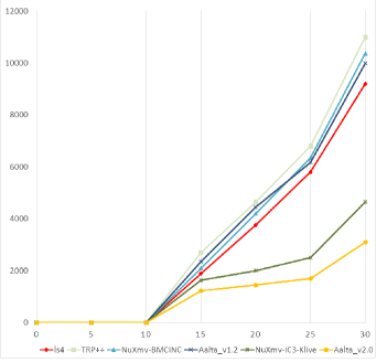
Figure 2: Results for LTL-satisfiability checking on Random Conjunction Formulas.

This section shows more experimental results on LTL-satisfiability checking. First we complete the results in Table 1 and list the results on satisfiable and unsatisfiable formulas separately, which are respectively shown in Table 2 and Table 3. Slightly different with Table 1, each cell of these two tables lists a tuple $\langle t,n\rangle$ where $n$ is the total number of solved formulas and $t$ is the total checking time for solving these $n$ cases (in seconds). In these two table Aalta_v2.0 is tested by using heuristics. The separation may help readers understand better of checking performance on satisfiability and unsatisfiability.

In additional to the schuppan-collected benchmarks, we also tested all solvers on the random conjunction formulas, which is proposed in [18]. A random conjunction formula $RC(n)$ has the form of $\bigwedge_{1\leq i\leq n}P_{i}(v_{1},v_{2},\ldots,v_{k})$, where $n$ is the number of conjunctive elements and $P_{i}(1\leq i\leq n)$ is a randomly chosen pattern formula used frequently in practice. The motivation is that typical temporal assertions may be quite small in practice. And what makes the LTL satisfiability problem often hard is that we need to check large collections of small temporal formulas, so we need to check that the conjunction of all input assertions is satisfiable. In our experiment, the number of $n$ varies from 1 to 30, and for each $n$ a set of 100 conjunctions formulas are randomly chosen. The experimental results are shown in Fig. 2. It shows that Aalta_v2.0 (with heuristic) performs best among tested solvers, and comparing to the second best solver (NuXmv), it achieves approximately the 30% speed-up.

Appendix 0.E SMT-based Temporal Reasoning

An additional motivation to base explicit temporal reasoning on SAT solving is the need to handle LTL formulas with assertional atoms, that is, atoms that are non-boolean state assertions, e.g., assertions about program variables, such as $k\leq 10$. Existing explicit temporal-reasoning techniques abstract such assertions as propositional atoms. Consider, for example, the LTL formula $\phi=\bigwedge_{1\leq i\leq n}F(k=i)$, which asserts that $k$ should assume all values between $1$ and $n$. By abstracting $k=i$ as $p_{i}$, we get the formula $\phi^{\prime}=\bigwedge_{1\leq i\leq n}Fp_{i}$, but the transition system for the abstract formula has $2^{n}$ states, while the transition system for the original formula has only $n$ states. This problem was noted, but not solved in [31], but it is obvious that reasoning about non-Boolean assertions requires reasoning at the assertion level. Basing explicit temporal reasoning on SAT solving, would enable us to lift it to the assertion level by using Satisfiability Modulo Theories (SMT) solving. SMT solving is a decision problem for logical formulas in combinations of background theories expressed in classical first-order logic. Examples of theories typically used are the theory of real numbers, the theory of integers, and the theories of various data structures such as lists, arrays, bit vectors, and others. SMT solvers have shown dramatic progress over the past couple of decades and are now routinely used in industrial software development [24].

So far, we described how to use SAT solving for checking satisfiability of propositional LTL formulas. And in this section we show that our approach can be extended to reason assertional LTL formulas. In many applications, we need to handle LTL formulas with assertional atoms, that is, atoms that are non-boolean state assertions, e.g., assertions about program variables. For example, Spin model checker uses temporal properties expressed in LTL using assertions about Promela state variables [14]. Existing explicit temporal-reasoning tools, e.g., SPOT [8], abstract such assertions as propositional atoms.

Recall that we utilize SAT solvers in our approach to compute assignments of formulas $\phi^{p}$ (with $\phi$ is in XNF). The states of transition system are then obtained from these assignments. When $\phi$ is an assertional LTL formula, the formula $\phi^{p}$ is not a propositional formula, but a Boolean combination of theory atoms, for an appropriate theory. Thus, our approach is still applicable, except that we need to replace the underlying SAT solver by an SMT solver.

Consider, for example the formula $\phi=(F(k=1)\wedge F(k=2))$. The XNF of $\phi$, i.e. $\mathit{xnf}(\phi)$, is $((v(F(k=1))\wedge(k=1))\vee(\neg v(F(k=1))\wedge XF(k=1)))\wedge((v(F(k=2))\wedge(k=2))\vee(\neg v(F(k=2))\wedge XF(k=2)))$. If we use a SAT solver, we can obtain an assignment such as $A=\{(k=1),v(F(k=1)),\neg XF(k=1),(k=2),v(F(k=2)),\neg XF(k=2)\}$, which is consistent propositionally, but inconsistent theory-wise. This can be avoided by using an SMT solver. Generally for a formula $\phi_{n}=\bigwedge_{1\leq i\leq n}F(k=i)$, there are $O(2^{n})$ states generated in the transition system by the SAT-based approach, but only $n$ states need to be generated. This can be achieved by replacing the SAT solver in our approach by an SMT solvers. The performance gap between the SAT-based approach and the SMT-based approach would be exponential. Indeed, SPOT performance on the formulas $\phi_{n}$ is exponential in $n$.

As proof of concept, we checked satisfiability of the formulas $\phi_{n}$, for $n=1,\ldots,100$, by Aalta_v2.0. We then replaced Minisat by Z3, a state-of-the-art SMT solver [24]. The performance results show indeed an exponential gap between the SAT-based approach and the SMT-based approach, which is shown in Fig. 3. (Of course, we also gain in correctness: the formula $F(k=1\wedge k=2)$ is satisfiable when considered propositionally, but unsatisfiable when considered assertionally.) Applying SMT-based techniques in other temporal-reasoning tasks, such as translating LTL to Büchi automata [11] or to runtime monitors [31], is a promising research direction.

Figure 3: Results for LTL-satisfiability checking on $\bigwedge_{1\leq i\leq n}F(k=i)$.

References

- [1] A. Bradley. SAT-based model checking without unrolling. In Ranjit Jhala and David Schmidt, editors, Verification, Model Checking, and Abstract Interpretation, volume 6538 of Lecture Notes in Computer Science, pages 70–87. Springer Berlin Heidelberg, 2011.
- [2] R. Cavada, A. Cimatti, M. Dorigatti, A. Griggio, A. Mariotti, A. Micheli, S. Mover, M. Roveri, and S. Tonetta. The nuxmv symbolic model checker. In CAV, pages 334–342, 2014.
- [3] K. Claessen and N. Sörensson. A liveness checking algorithm that counts. In Gianpiero Cabodi and Satnam Singh, editors, FMCAD, pages 52–59. IEEE, 2012.
- [4] E.M. Clarke, O. Grumberg, and D. Peled. Model Checking. MIT Press, 1999.
- [5] C. Courcoubetis, M.Y. Vardi, P. Wolper, and M. Yannakakis. Memory efficient algorithms for the verification of temporal properties. Formal Methods in System Design, 1:275–288, 1992.
- [6] M. d’Agostino. Tableau methods for classical propositional logic. In Handbook of tableau methods, pages 45–123. Springer, 1999.
- [7] N. Daniele, F. Guinchiglia, and M.Y. Vardi. Improved automata generation for linear temporal logic. In Proc. 11th Int. Conf. on Computer Aided Verification, volume 1633 of Lecture Notes in Computer Science, pages 249–260. Springer, 1999.
- [8] A. Duret-Lutz and D. Poitrenaud. SPOT: An extensible model checking library using transition-based generalized büchi automata. In Proc. 12th Int’l Workshop on Modeling, Analysis, and Simulation of Computer and Telecommunication Systems, pages 76–83. IEEE Computer Society, 2004.
- [9] N. Eén and N. Sörensson. An extensible SAT-solver. In SAT, pages 502–518, 2003.
- [10] M. Fisher. A normal form for temporal logics and its applications in theorem-proving and execution. Journal of Logic and Computation, 7(4):429–456, 1997.
- [11] R. Gerth, D. Peled, M.Y. Vardi, and P. Wolper. Simple on-the-fly automatic verification of linear temporal logic. In P. Dembiski and M. Sredniawa, editors, Protocol Specification, Testing, and Verification, pages 3–18. Chapman & Hall, 1995.
- [12] F. Giunchiglia and R. Sebastiani. Building decision procedures for modal logics from propositional decision procedure - the case study of modal K. In Proc. 13th Int’l Conf. on Automated Deduction, volume 1104 of Lecture Notes in Computer Science, pages 583–597. Springer, 1996.
- [13] K. Heljanko, T. Junttila, and T. Latvala. Incremental and complete bounded model checking for full PLTL. In K. Etessami and S. Rajamani., editors, Computer Aided Verification, volume 3576 of Lecture Notes in Computer Science, pages 98–111. Springer Berlin Heidelberg, 2005.
- [14] G.J. Holzmann. The SPIN Model Checker: Primer and Reference Manual. Addison-Wesley, 2003.
- [15] U. Hustadt and B. Konev. Trp++ 2.0: A temporal resolution prover. In In Proc. CADE-19, LNAI, pages 274–278. Springer, 2003.
- [16] T. Larrabee. Test pattern generation using boolean satisfiability. IEEE Trans. on Computer-Aided Design of Integrated Circuits and Systems, 11(1):4–15, 1992.
- [17] J. Li, G. Pu, L. Zhang, M. Y. Vardi, and J. He. Fast LTL satisfiability checking by SAT solvers. CoRR, abs/1401.5677, 2014.
- [18] J. Li, L. Zhang, G. Pu, M. Vardi, and J. He. LTL satisfibility checking revisited. In The 20th International Symposium on Temporal Representation and Reasoning, pages 91–98, 2013.
- [19] S. Malik and L. Zhang. Boolean satisfiability from theoretical hardness to practical success. Commun. ACM, 52(8):76–82, 2009.
- [20] Z. Manna and A. Pnueli. The Temporal Logic of Reactive and Concurrent Systems: Specification. Springer, 1992.
- [21] J. Marques-Silva and I. Lynce. On improving MUS extraction algorithms. In K. Sakallah and L. Simon, editors, Theory and Applications of Satisfiability Testing - SAT 2011, volume 6695 of Lecture Notes in Computer Science, pages 159–173. Springer Berlin Heidelberg, 2011.
- [22] K. McMillan. Interpolation and SAT-based model checking. In Jr. Hunt, WarrenA. and Fabio Somenzi, editors, Computer Aided Verification, volume 2725 of Lecture Notes in Computer Science, pages 1–13. Springer Berlin Heidelberg, 2003.
- [23] K.L. McMillan. Symbolic Model Checking. Kluwer Academic Publishers, 1993.
- [24] L. De Moura and N. Bjørner. Z3: An efficient SMT solver. In Proceedings of the Theory and Practice of Software, 14th International Conference on Tools and Algorithms for the Construction and Analysis of Systems, TACAS’08/ETAPS’08, pages 337–340, Berlin, Heidelberg, 2008. Springer-Verlag.
- [25] A. Pnueli. The temporal logic of programs. In Proc. 18th IEEE Symp. on Foundations of Computer Science, pages 46–57, 1977.
- [26] K.Y. Rozier and M.Y. Vardi. LTL satisfiability checking. Int’l J. on Software Tools for Technology Transfer, 12(2):123–137, 2010.
- [27] V. Schuppan and L. Darmawan. Evaluating LTL satisfiability solvers. In Proceedings of the 9th international conference on Automated technology for verification and analysis, AVTA’11, pages 397–413. Springer-Verlag, 2011.
- [28] S. Schwoon and J. Esparza. A note on on-the-fly verification algorithms. In Proc. 11th Int’l Conf. on Tools and Algorithms for the Construction and Analysis of Systems, Lecture Notes in Computer Science 3440, pages 174–190. Springer, 2005.
- [29] F. Somenzi and R. Bloem. Efficient Büchi automata from LTL formulae. In Proc. 12th Int. Conf. on Computer Aided Verification, volume 1855 of Lecture Notes in Computer Science, pages 248–263. Springer, 2000.
- [30] M. Suda and C. Weidenbach. A PLTL-prover based on labelled superposition with partial model guidance. In Automated Reasoning, volume 7364 of Lecture Notes in Computer Science, pages 537–543. Springer Berlin Heidelberg, 2012.
- [31] D. Tabakov, K.Y. Rozier, and M. Y. Vardi. Optimized temporal monitors for SystemC. Formal Methods in System Design, 41(3):236–268, 2012.
- [32] M. Vardi. On the complexity of epistemic reasoning. In Proceedings of the Fourth Annual Symposium on Logic in Computer Science, pages 243–252, Piscataway, NJ, USA, 1989. IEEE Press.
- [33] M.Y. Vardi. Unified verification theory. In B. Banieqbal, H. Barringer, and A. Pnueli, editors, Proc. Temporal Logic in Specification, volume 398, pages 202–212. Springer, 1989.
- [34] M.Y. Vardi and P. Wolper. An automata-theoretic approach to automatic program verification. In Proc. 1st IEEE Symp. on Logic in Computer Science, pages 332–344, 1986.