Autocovariance estimation in regression with a discontinuous signal and $m$-dependent errors: A difference-based approach

Abstract.

We discuss a class of difference-based estimators for the autocovariance in nonparametric regression when the signal is discontinuous (change-point regression), possibly highly fluctuating, and the errors form a stationary $m$-dependent process. These estimators circumvent the explicit pre-estimation of the unknown regression function, a task which is particularly challenging for such signals. We provide explicit expressions for their mean squared errors when the signal function is piecewise constant (segment regression) and the errors are Gaussian. Based on this we derive biased-optimized estimates which do not depend on the particular (unknown) autocovariance structure. Notably, for positively correlated errors, that part of the variance of our estimators which depends on the signal is minimal as well. Further, we provide sufficient conditions for $\sqrt{n}$-consistency; this result is extended to piecewise Hölder regression with non-Gaussian errors.

We combine our biased-optimized autocovariance estimates with a projection-based approach and derive covariance matrix estimates, a method which is of independent interest. Several simulation studies as well as an application to biophysical measurements complement this paper.

1. Introduction

In nonparametric regression with correlated errors,

$$y_{i}=f(x_{i})+\varepsilon_{i},\quad i=1,\ldots,n,$$ (1.1)

where $(x_{i})$ are the sampling points, $f$ is an unknown mean function or signal, and $(\varepsilon_{i})$ are zero mean stationary time series errors, the autocovariance $\gamma_{h}=\mathsf{E}[\varepsilon_{1}\,\varepsilon_{1+h}]$, $h=0,1,\ldots$, plays a prominent role for various tasks. When the signal $f$ is smooth, the autocovariance appears, e.g., in the asymptotic variance of kernel estimators of $f$ and is important for bandwidth selection and for inferential procedures, cf. Opsomer et al., (2001). In general, knowledge of the autocovariance, and in particular of the variance $\sigma^{2}=\gamma_{0}$, is required for efficient signal estimation, e.g. in wavelet-based estimation the autocovariance can be used for improved thresholding of the empirical wavelet coefficients, cf. Johnstone and Silverman, (1997), Von Sachs and MacGibbon, (2000), Kovac and Silverman, (2000). Additionally, when the signal is discontinuous, which will be considered in this paper, the autocovariance function is required to provide efficient estimates and confidence regions for the location of the discontinuities as well as the magnitude of their corresponding jumps, see Section 7.2 for an example. Autocovariance estimation under a discontinuous and potentially highly fluctuating signal, however, is a notoriously difficult task in general and some knowledge about the dependence structure is necessary. Therefore, throughout this paper we will consider zero mean, stationary, $m$-dependent errors, i.e., $\gamma_{h}=0$ for $|h|>m$; $\gamma_{m}\neq 0$. Although $m$-dependency ensures that the autocovariance function is zero starting at lag $m+1$, this characteristic of our error model can often be construed as a convenient proxy to more general situations, e.g. when the autocovariance function decays exponentially with increasing lag.

Regression models with discontinuous signal and $m$-dependent errors as considered in this paper are of relevance in several areas of application. Figure 1 displays time series from two common biophysical measurements: (A) recordings of an ion channel trace and (B) the trajectory of a molecular dynamic protein. For (A), the mean is typically modelled with a locally constant signal (also called change-point segment regression) according to the openings and closings of the channel, cf. VanDongen, (1996), and $m$-dependence results from the low-pass filter utilized to digitize ion channel measurements, cf. Hotz et al., (2013). For (B) a more flexible signal assumption (piecewise smooth change-point regression) seems in order and often $m$-dependence can be confirmed empirically.

A

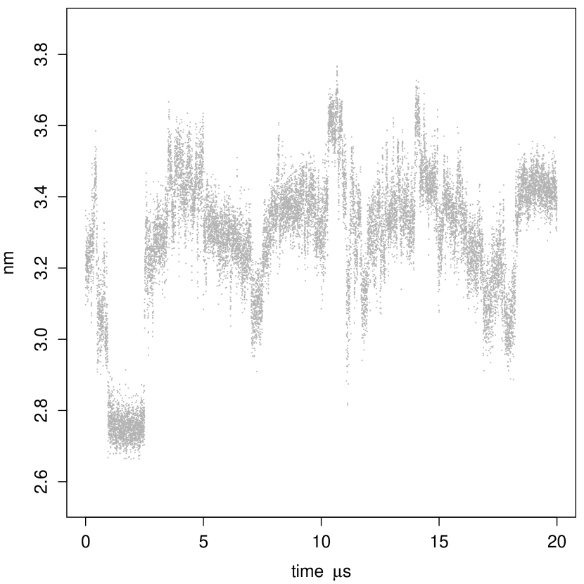
B

Figure 1. (A) 60 s of gramicidin A, see Section 7 for further details about this dataset. (B) 20000 ns of the trajectory of the distance between a backbone atom and the first center of mass of water channel AQY1, cf. Krivobokova et al., (2012) for further details.

The contributions of this paper are also relevant for change-point estimation and detection which have been investigated extensively in the particular case of independent errors, see e.g. Page, (1954, 1955), Dümbgen, (1991), Brodsky and Darkhovsky, (1993) and Carlstein et al., (1994) for some early references. More recently, and arguably motivated by large scale applications, e.g. from genetics, the focus has been on the recovery of signals with a potentially large number of change-points, see e.g. Olshen et al., (2004), Fearnhead and Liu, (2007), Spokoiny, (2009), Harchaoui and Lévy-Leduc, (2010), Killick et al., (2012), Siegmund, (2013), Frick et al., (2014), Du et al., (2016) and Li et al., (2016) among many others. For serially correlated errors, change-points estimates have been primarily investigated asymptotically and when the number of change-points is finite (but unknown) see e.g. Davis et al., (2006), Fryzlewicz and Subba Rao, (2014), Preuß et al., (2015) and Chakar et al., (2016). To some extent, such an asymptotic analysis resembles finite sample situations when the number of change-points is small (relative to the sample size) and variance-covariance estimation becomes less cumbersome (Picard, (1985), Hušková et al., (2007)). Autocovariance estimation may even be disregarded for consistent change-point estimation over large classes of dependency structures (Lavielle and Moulines, (2000), Bardet et al., (2012)).

In contrast, in this paper we mainly adopt a non-asymptotic perspective motivated by highly fluctuating signals having a potentially large number of change-points as it is known that this will increase the finite sample bias of any standard variance-covariance estimate. Hence, subsequent use of these biased estimates may significantly reduce the efficiency of change-point statistics, cf. Eqs. (13)-(15) of Jandhyala et al., (2013). As we will show later on, even when the number of change-points increases with the sample size, it is still possible to account for bias-reducing and $\sqrt{n}$-consistent estimates for $\gamma_{(\cdot)}$. This is reflected by the fact that estimation of $\gamma_{(\cdot)}$ is simpler than that of the entire signal $f$, which is well-known for $\gamma_{0}=\sigma^{2}$ in the independent case (e.g. Spokoiny, (2002)).

In summary, in those situations when the signal fluctuation becomes dominant (which will be made precise later on), pre-estimation of the signal $f$ is notoriously difficult and direct estimation of $\gamma_{(\cdot)}$ becomes pertinent. This paradigm is well known, in particular, for independent noise, i.e. for estimation of the variance $\sigma^{2}$. For this task, difference-based estimators provide a simple and practical solution: a difference sequence $\{\Delta_{i}\}$ is a sequence of real numbers such that

$$\sum\,\Delta_{i}=0,\quad\sum\Delta_{i}^{2}=1.$$ (1.2)

Assume that $\Delta_{i}=0$ for $i<-l_{1}$ and $i>l_{2}$, and $\Delta_{-l_{1}}\,\Delta_{l_{2}}\neq 0$ with $l_{1},l_{2}\geq 0$. Then $l=l_{1}+l_{2}$ is called the order of the sequence; usually $l_{1}=0$ and $l_{2}=l$. Following Hall et al., (1990) a difference-based estimate of $\sigma^{2}$ has the form

$$\hat{\sigma}^{2}=(n-l)^{-1}\,\sum_{k=l_{1}+1}^{n-l_{2}}\left(\sum_{i}\,\Delta_{i}\,y_{i+k}\right)^{2}.$$ (1.3)

When the signal is smooth, estimators of this type have been investigated extensively see e.g. Rice, (1984), Gasser et al., (1986), Müller and Stadtmüller, (1987), Dette et al., (1998), Spokoiny, (2002), Brown et al., (2007), Tong et al., (2013), Dai et al., (2015). As argued by Munk et al., (2005) and others, a particular appeal of these estimators is that their weights can be adapted to high fluctuation of the signal, i.e. for bias reduction. As we will see in this paper, this feature makes difference-based estimators particularly useful also in applications with correlated errors where the signal exhibits high fluctuation and discontinuities.

Difference-based estimators have also been used in nonparametric regression with stationary errors. For instance, Müller and Stadtmüller, (1988) proposed estimators based on differences of first order to estimate (invertible) linear transformations of the variance-covariance matrix of stationary $m$-dependent errors. Herrmann et al., (1992) suggested differences of second order to estimate the zero frequency of the spectral density of stationary processes with short-range dependence. For autoregressive errors, Hall and Van Keilegom, (2003) proposed $\sqrt{n}$-consistent and, under normality, efficient autocovariance estimates. Under some mixing conditions, Park et al., (2006) suggested to estimate the autocovariance function applying difference-based estimators of first order to the residuals of a kernel-based fit of the signal. Most close to our work is Zhou et al., (2015), who provide an optimal difference-based estimate of the variance $\sigma^{2}=\gamma_{0}$ for smooth nonparametric regression when the errors are correlated. Their optimized weights, however, depend on the remaining values of the autocovariance function, i.e. $\gamma_{h}$, $h\neq 0$, which in general are unknown. In contrast, in this paper we estimate the entire autocovariance function and our estimates depend solely on $m$. All the methods just discussed have been analyzed for smooth signals and to the best of our knowledge, derivation of optimal weights for autocovariance difference-based estimates in the case of a discontinuous and highly fluctuating signal still remains elusive and becomes the main focus of our work.

Summarizing this paper, we begin by suggesting the use of difference-based estimators of the autocovariance of the error process in nonparametric regression (1.1). Then we show that for $m$-dependent errors we need to use differences of gap $m+1$. We obtain finite-sample results for the mean squared error ($\mathsf{MSE}$) of these estimators. This $\mathsf{MSE}$ includes a bias term which depends on the unknown regression function $f$, in situations where $f$ fluctuates substantially this term could dominate. We show that to minimize this bias term (and that part of the variance which depends on $f$ as well) we should use estimators based on only first or second order differences and give explicit forms for the optimal choice of weights in the difference-based estimators. Further, we provide sufficient conditions for $\sqrt{n}$-consistency; this result is extended to piecewise Hölder regression with non-Gaussian errors. A more detailed account of these and other results is presented in the next section. The theory is complemented by simulation studies, a data example, and statistical software for autocovariance estimation.

2. Main results

As a prototypical example of a regression model with a discontinuous signal we consider for the moment (1.1) with a signal $f$ that is locally constant (change-point segment regression) and hence admits the representation

$$f(x)=\sum_{j=0}^{K-1}\,a_{j}{1\textnormal{l}}_{[\tau_{j},\tau_{j+1})}(x),\quad x\in[0,1),\quad a_{j}\neq a_{j+1}.$$ (2.1)

Here the change-points of $f$, $0=\tau_{0}<\tau_{1}<\cdots<\tau_{K-1}<\tau_{K}=1$, its levels $(a_{j})_{0\leq j\leq K-1}$, and the number of discontinuities $K\in\mathbb{N}$ are unknown and can be potentially large. Since for large enough $K$ any discretized function can be represented as in (2.1), this equation describes a wide class of signals. For simplicity of presentation we will assume that the sampling points $(x_{i})$ are equally spaced on $[0,1)$, i.e., $x_{i}=i/n$. Further, $f_{i}$ will denote $f(x_{i})$.

2.1. Autocovariance estimation

Now we introduce the class of difference-based estimators to be considered for $m$-dependent errors. Let ${\bf Y}$ denote the vector of observations $y_{i}$ following (1.1). For $1\leq lh<n$, a generalized difference-based estimator of order $l$ and gap $h$ is a random quadratic form

$${\bf Q}_{h}({\bf Y},\boldsymbol{w}_{l})=\frac{1}{P(\boldsymbol{w}_{l})(n-lh)}\sum_{i=1}^{n-lh}(d_{0}y_{i}+d_{1}y_{i+h}+d_{2}y_{i+2\,h}\ldots+d_{l}\,y_{i+l\,h})^{2},$$ (2.2)

where $\boldsymbol{w}_{l}=(d_{0}\quad d_{1}\quad\cdots\quad d_{l})^{\top}\in\mathbb{R}^{l+1}$ is a vector of numbers (weights) satisfying

$$\sum_{i=0}^{l}\,d_{i}=0,$$ (2.3)

and $P(\boldsymbol{w}_{l})=\sum_{i=0}^{h}d_{i}^{2}$. Setting $h=1$ in (2.2) we get difference-based estimators of order $l$, cf. Eq.(1.3). For $l=1$ and $\boldsymbol{w}_{1}=(1\quad-1)^{\top}\in\mathbb{R}^{2}$, $P(\boldsymbol{w}_{1})=2$ and for $1\leq h<n$ we get the ordinary difference-based estimator of gap $h$ (for $h=1$ see Rice, (1984)):

$$\widehat{\delta}^{(h)}=\frac{1}{2(n-h)}\,\sum_{i=1}^{n-h}\left(y_{i}-y_{i+h}\right)^{2}.$$ (2.4)

Note that for independent errors in (1.1), $\mathsf{E}[\widehat{\delta}^{(h)}]=\gamma_{0}+o(1)$ provided $\sum_{i=1}^{n-h}(f_{i}-f_{i+h})^{2}=o(n)$ and we can use the estimator (2.4) to get asymptotically unbiased estimates of the variance. In contrast, for stationary errors the situation becomes more complicated as then $\mathsf{E}[\widehat{\delta}^{(h)}]=\gamma_{0}-\gamma_{h}+o(1)$.

We will show for the change-point segment model (2.1) (Theorem 5 of Section 3.1) that for $m$-dependent errors any estimator of the variance $\gamma_{0}=\sigma^{2}$ whose $\mathsf{MSE}$ tends to 0 and that satisfies (2.2)-(2.3) must have gap $h$ at least $m+1$. Therefore, we will focus on this type of variance estimators in the following. We will further restrict ourselves to estimators of first or second order, see Lemma 1 below for justification of this. We commence now a discussion about the $\mathsf{MSE}$ of this class of estimators.

Let $n_{m}=n-2(m+1)$ and w.l.o.g. set $d_{0}=1$, then estimators for $\gamma_{0}$ based on differences of second order ($l=2$) and gap $m+1$ in (2.2) can be written as

$$~{}\widehat{\gamma}^{(m)}_{0}(d)=\frac{(1+d+d^{2})^{-1}}{2\,n_{m}}\,\sum_{i=1}^{n_{m}}\left(y_{i}-(1+d)y_{i+(m+1)}+d\,y_{i+2(m+1)}\right)^{2},\quad d\in\mathbb{R},$$ (2.5)

using (2.3). Combining the ordinary difference-based estimator of gap $h$, cf. (2.4), with (2.5) we will estimate the remaining values of the autocovariance function $\gamma_{h}$, $h=1,\ldots,m$. Namely,

$$~{}\widehat{\gamma}_{h}^{(m)}(d)=\widehat{\gamma}^{(m)}_{0}(d)-\widehat{\delta}^{(h)},\quad d\in\mathbb{R},\quad h=1,\ldots,m.$$ (2.6)

Here $d\in\mathbb{R}$ is a parameter to be optimized later on. In order to present our first result we need to introduce the quadratic variation of $f$ in (2.1):

$$~{}J_{K}:=\sum_{j=0}^{K-1}(a_{j+1}-a_{j})^{2}.$$ (2.7)

Theorem 1.

Suppose that in the segment regression model (1.1)-(2.1) the noise $(\varepsilon_{i})_{1\leq i\leq n}$ is a sample from a zero mean, $m$-dependent, stationary Gaussian process with autocovariance function $\gamma_{h}=\mathsf{E}[\varepsilon_{1}\,\varepsilon_{1+h}]$, $h=0,\ldots,m$. Additionally, assume that the change-points of $f$, $0=\tau_{0}<\tau_{1}<\cdots<\tau_{K-1}<\tau_{K}=1$, satisfy that

$$\min_{1\leq i\leq{K-1}}|\tau_{i+1}-\tau_{i}|>4(m+1)/n.$$ (2.8)

Then, for $m\geq 1$

$$~{}\mathsf{MSE}[\widehat{\gamma}_{0}^{(m)}(d)]=\underbrace{n^{-2}\,p_{0}^{2}(d)\,J_{K}^{2}}_{\mathsf{BIAS}^{2}}+\underbrace{n^{-2}\left(p_{1}(d;\gamma_{(\cdot)})\,\gamma_{0}\,J_{K}+n\,p_{2}(d;\gamma_{(\cdot)})+p_{3}(d;\gamma_{(\cdot)})\right)}_{\mathsf{VAR}},$$ (2.9)

and for $h=1,\ldots,m$

$$~{}\mathsf{MSE}[\widehat{\gamma}_{h}^{(m)}(d)]=\underbrace{n^{-2}\,(p_{0}^{\ast})^{2}(d)\,J_{K}^{2}}_{\mathsf{BIAS}^{2}}+\underbrace{n^{-2}\left(p_{1}^{\ast}(d;\gamma_{(\cdot)})\,J_{K}+n\,p_{2}^{\ast}(d;\gamma_{(\cdot)})+p_{3}^{\ast}(d;\gamma_{(\cdot)})\right)}_{\mathsf{VAR}}.$$ (2.10)

See Section 3.2 for explicit expressions of $p_{0}$, $p_{0}^{\ast}$, $p_{1}$, $p_{1}^{\ast}$, $p_{2}$, $p_{2}^{\ast}$, $p_{3}$ and $p_{3}^{\ast}$. We remark that Gaussianity is only needed to get the variance explicitly.

Remark 1.

As mentioned above for simplicity we are considering equally spaced observations sampled from the unit interval at rate $1/n$. Note, however, that our results can be transferred to general sampling points as we provide the finite sample $\mathsf{MSE}$s (2.9)-(2.10) and the only restriction is (2.8) which transfers to general sampling points by replacing $\tau_{j}$ by $\lfloor n\tau_{j}\rfloor$, where $\lfloor x\rfloor$ denotes the integer part of $x$.

Now let us discuss Theorem 1. As an immediate consequence we deduce that the influence of $f$ over the $\mathsf{MSE}$s (2.9)-(2.10) only appears through its quadratic variation $J_{K}$ (2.7). Let us first consider (2.9). Here the bias consists of $n^{-1}\,p_{0}(\cdot)$, a rational function, times $J_{K}$. We can further define the extended bias, $\mathsf{BIAS}^{\ast}$, of $\widehat{\gamma}_{0}^{(m)}(d)$ as the part of the $\mathsf{MSE}$ in (2.9) that depends on $f$:

$$\mathsf{BIAS}^{\ast}[\widehat{\gamma}_{0}^{(m)}(d)]:=n^{-2}\left[p_{0}^{2}(d)\,J_{K}^{2}+p_{1}(d;\gamma_{(\cdot)})\,\gamma_{0}\,J_{K}\right].$$ (2.11)

In order to justify our definition of extended bias, note that unlike $p_{1}$, the rational functions $p_{2}(\cdot;\gamma_{(\cdot)})$ and $p_{3}(\cdot;\gamma_{(\cdot)})$ do not align with $f$ and these functions affect the part of the variance which solely depends on the autocovariance. A similar analysis and conclusions can be made for the estimators $\widehat{\gamma}_{h}^{(m)}(d)$ in (2.10).

In view of (2.9) and (2.10) we deduce that for highly oscillating and discontinuous signals, in (2.1), e.g. for large $K$, the influence of $J_{K}$ over the $\mathsf{MSE}$s may become dominant and might not be negligible even for very large sample sizes. On the contrary, the influence of the unknown autocovariance function $\gamma_{(\cdot)}$ over the $\mathsf{MSE}$s is comparably small in this situation.

In light of the above we focus on finding variance estimates in (2.5) and autocovariance estimates in (2.6) whose $\mathsf{MSE}$s (see Theorem 1) have minimal influence from $J_{K}$ (and hence from $f$). Our main results on autocovariance estimation for change-point regression with stationary $m$-dependent errors are stated now.

Estimation of $\gamma_{0}$. From Theorem 1 we get that $\mathsf{BIAS}[\widehat{\gamma}_{0}^{(m)}(d)]=n^{-1}p_{0}(d)\,J_{K}$, see (2.9). Since for $m\in\mathbb{N}$, $\min_{d\in\mathbb{R}}p_{0}(d)=p_{0}(1)=((m+1)/3)^{2}$, for details see (3.3), we have proven the following:

Theorem 2.

Let $\widehat{\gamma}_{0}^{(m)}(d)$ be the difference-based estimator given by (2.5). Suppose that in the segment regression model (1.1)-(2.1)-(2.8), the noise $(\varepsilon_{i})_{1\leq i\leq n}$ is a sample from a zero mean, $m$-dependent, stationary process. Then for $m\geq 1$, $\mathsf{BIAS}[\widehat{\gamma}_{0}^{(m)}(d)]$ is minimized at $d=1$, i.e., by the estimator

$$\widehat{\gamma}_{0}^{(m)}(1)=\frac{1}{6\,n_{m}}\,\sum_{i=1}^{n_{m}}\left(y_{i}-2\,y_{i+(m+1)}+y_{i+2(m+1)}\right)^{2},\quad n_{m}=n-2(m+1).$$ (2.12)

Note that in Theorem 2 a normal error assumption is not needed. Already Herrmann et al., (1992) have suggested this estimator in the context of nonparametric regression with a smooth signal and stationary errors. Note that Theorem 2 provides further justification for its use particularly when the signal is discontinuous. In fact, assuming further that the correlation is non-negative, we found that even the extended bias of $\widehat{\gamma}_{0}^{(m)}(d)$, is minimized at $d=1$. More precisely we get the following result whose proof can be found in Section 3.2.

Theorem 3.

Suppose that the conditions of Theorem 1 hold. Assume, additionally, that the autocovariance function of the noise $(\varepsilon_{i})_{1\leq i\leq n}$ belongs to either of the following classes:

1. $\gamma_{h}=\rho\,\gamma_{0}$, for $h=1,\ldots,m$ such that

   $$1+2\,\rho\,\sum_{h=1}^{m}\,\cos(h\,\lambda)\geq 0,\quad\forall\lambda\in[-\pi,\pi].$$ (2.13)

2. $\gamma_{h}\geq 0$ for $h=1,\ldots,m$.

Then for $m\geq 1$, the estimator $\widehat{\gamma}_{0}^{(m)}(1)$ in (2.12) minimizes the extended bias $\mathsf{BIAS}^{\ast}[\widehat{\gamma}_{0}^{(m)}(d)]$, cf. (2.11).

Eq. (2.13) ensures that the function $\gamma_{h}=\rho\,\gamma_{0}$ for $h=1,\ldots,m$ and zero otherwise, is the autocovariance of a zero mean, stationary, $m$-dependent process, cf. Corollary 4.3.2 of Brockwell and Davis, (2006).

Estimation of $\gamma_{h}$, $h=1,\ldots,m$. We will show that the following weights optimize the bias of estimators given by (2.6):

$$d_{h,m}=\begin{cases}1&\mbox{ for }h<\frac{2}{3}(m+1)\\ \frac{h\pm\sqrt{h^{2}-4(m+1-h)^{2}}}{2(m+1-h)}&\mbox{ otherwise }\end{cases}.$$ (2.14)

Theorem 4.

Suppose that the conditions of Theorem 2 hold. Then for $m\geq 1$, $\mathsf{BIAS}[\widehat{\gamma}_{h}^{(m)}(d)]$ is minimized at $d_{h,m}$, cf. (2.14). In particular, for those values of $h$ such that $h\geq\frac{2}{3}(m+1)$, $\widehat{\gamma}_{h}^{(m)}(d_{h,m})$ is an unbiased estimate of $\gamma_{h}$.

Proof.

Since $\mathsf{BIAS}[\widehat{\gamma}_{h}^{(m)}(d)]={p_{0}^{\ast}(d)}J_{K}/n$, cf. Theorem 1, where $p_{0}^{\ast}(d)=p_{0}(d)-h/2$, cf. (3.8), we only need to minimize $p_{0}^{\ast}(\cdot)$ w.r.t. $d$. For $3h\geq 2(m+1)$, $d_{h,m}$, cf. Eq. (2.14), is a root of $p_{0}^{\ast}$. For $3h<2(m+1)$, straightforward calculations yield that $d=1$ is a global minimum of $p_{0}^{\ast}$ on $\mathbb{R}$. This completes the proof. ∎

Observe that the underlying autocovariance $\gamma_{(\cdot)}$ does not appear in the expression for $\widehat{\gamma}_{h}^{(m)}(d_{h,m})$, $h=1,\ldots,m$. In contrast, the corresponding extended bias of $\widehat{\gamma}_{h}^{(m)}(d)$, $d\in\mathbb{R}$, depends on the unknown $\gamma_{(\cdot)}$ in an intricate fashion, cf. Eq. (2.10)-(3.10)-(3.11)-(3.12), hence full minimization of this function is practically infeasible.

In summary, we find that the difference-based estimates given by (2.12) and (2.14) are bias-reducing for the autocovariance of wide classes of stationary $m$-dependent processes and discontinuous signals. Additionally, under Gaussianity and for non-negative correlation, (2.12) is even extended-bias-optimal. Moreover, Theorem 7 of Section 4 establishes that for piecewise Hölder continuous signal (which includes segment regression (2.1)) with general (non-Gaussian) errors whose all moments up to order 4 are stationary, the estimates (2.12)-(2.14) are $\sqrt{n}$-consistent for $\gamma_{(\cdot)}$ as long as the number of discontinuities $K_{n}=o(\sqrt{n})$.

2.2. Covariance matrix estimation

Let $\widehat{\Gamma}$ be the $n\times n$ symmetric Toeplitz matrix whose first $m+1$ entries of its first row are filled with $\widehat{\gamma}_{h}^{(m)}(d_{h,m})$, $h=0,1,\ldots,m$, cf. Eqs. (2.12)-(2.14), and the remaining $n-(m+1)$ entries are zero. As in general, pointwise autocovariance estimates $\widehat{\gamma}_{h}$, $h=0,1,\ldots,m$, may lead to a covariance matrix estimate which is not positive definite, cf. Hall and Van Keilegom, (2003), $\widehat{\Gamma}$ may not be the exception. In order to overcome this problem we propose a projection-based estimator. Define

$$\widehat{\Gamma}^{\ast}=P_{\mathcal{C}_{n}^{(m)}}(\widehat{\Gamma}):=\operatorname*{argmin}\{\|\widehat{\Gamma}-\Gamma^{(m)}\|_{F}:\Gamma^{(m)}\in\mathcal{C}_{n}^{(m)}\},$$ (2.15)

that is, the unique projection of $\widehat{\Gamma}$ onto $\mathcal{C}_{n}^{(m)}$, the closed convex set of all $n\times n$ symmetric, positive semidefinite, $(m+1)$-banded Toeplitz matrices. In (2.15), $\|\cdot\|_{F}$ denotes the Frobenius norm. We show that the projection-based estimate $\widehat{\Gamma}^{\ast}$ always has smaller mean squared error than the pointwise-based estimate $\widehat{\Gamma}$, cf. Theorem 8 in Section 5. This theorem might be of interest on its own since it relies on a general projection principle which can be applied to any ensemble of individual autocovariance estimators to obtain a symmetric, positive semidefinite Toeplitz (covariance) matrix estimate. Our final autocovariance matrix estimate $\widehat{\Gamma}^{\ast}$ in (2.15) can be computed numerically by a Dykstra-type alternating projection algorithm which we will detail in Section 5.1.

2.3. Numerical studies

Finite sample properties of our bias-reducing autocovariance estimators (2.12)-(2.14) are investigated in a series of simulations in Section 6 and compared to other estimators from the literature: Section 6.1 assesses the performance of these estimates for autocorrelation estimation, their robustness against normal distributed errors is also studied; robustness against the assumption of a piecewise constant signal is explored in Section 6.2. When the signal is discontinuous we found that our estimates outperform all the others under comparison. For smooth signals and positive correlation our estimates are competitive to some optimized kernel-based estimates.

2.4. Applications

In Section 7.1 we analyze the dependence structure of the data example shown in Figure 1A. We found a $6$-dependent process as appropriate and estimate its autocorrelation. We found that is in close agreement to that obtained by theoretical considerations from low-pass filtering. Although in this paper we only considered an application on biophysical measurements, we stress that our method may proven useful for many other areas such as the analysis of financial time series or sequential data in genetics. Finally, in Section 7.2 we show how our estimates can be used to improve considerably the estimation accuracy in the $m$-dependent case of a change-point estimator initially designed for independent data.

2.5. Software and Supporting Information

The methods discussed in this paper are available in the R package dbacf (http://www.stochastik.math.uni-goettingen.de/dbacf). In this software we have implemented the estimates (2.12)-(2.14) (see function dbacf) as well as the alternating projection algorithm from Section 5 leading to $\widehat{\Gamma}^{\ast}$ (see nearPDToeplitz). We defer the proofs of most of our results to the Supporting Information of this paper.

3. Optimization of difference-based estimators of autocovariance function

In what follows we will say that an estimate $W_{n}$ is consistent if $\mathsf{MSE}[W_{n}]\to 0$ as $n\to\infty$.

3.1. On the consistency of generalized difference-based estimators for variance of $m$-dependent processes

The next theorem highlights that in a change-point segment regression with zero mean, stationary, $m$-dependent errors, consistent estimation of the variance $\gamma_{0}$ based on difference schemes already restricts this class to estimators with gap $h$ at least $m+1$, see (2.2). Some technical details are deferred to Appendix A.1.

Theorem 5.

In the segment regression model (1.1)-(2.1)-(2.8) with zero mean, $m$-dependent, stationary errors, any consistent difference-based estimator for the variance $\gamma_{0}$ given by (2.2)-(2.3), has necessarily gap at least $m+1$. More precisely, let $g$ and $m$ be fixed integers with $g\geq m$ and assume that there exists an integer $N>1$ such that $n=N(g+1)$. Then, in (2.2), the vector of weights $\boldsymbol{w}_{n}$ must have the form:

$$\boldsymbol{w}_{n}=(\boldsymbol{v}_{0}\quad\boldsymbol{v}_{1}\quad\cdots\quad\boldsymbol{v}_{N-1})^{\top}\in\mathbb{R}^{n},$$

where $\boldsymbol{v}_{i}=(d_{i\,\cdot\,g}\quad 0\quad\cdots\quad 0)^{\top}\in\mathbb{R}^{g+1}$, $i=0,\ldots,N-1$; $d_{0}\neq 0$, $d_{k\,\cdot\,g}\neq 0$ for some $1\leq k\leq N-1$, and $\sum_{j=0}^{N-1}d_{j\,\cdot\,g}=0$. Here $j\cdot g$ denotes the multiplication of the index $j$ by the integer $g$.

Idea of proof.

Since a consistent estimate is necessarily asymptotically unbiased, our line of argument consists of showing that for any difference-based estimate satisfying (2.2)-(2.3) to be an asymptotically unbiased estimate of $\gamma_{0}$, it is necessary that its gap be at least $m+1$. The technical details of the proof can be found in Appendix A.1. ∎

A key part of the proof of Theorem 5 consists of computing the bias of a generalized difference-based estimator of order $l$ and gap 1. This is provided by Lemma 1 below and in order to present it now we introduce some notation. Recall that $f_{i}$ denotes $f(x_{i})$ and for $i<n-l$, $f_{i:(i+l)}$ denotes the vector $(f_{i}\quad f_{i+1}\quad\cdots\quad f_{i+l})^{\top}\in\mathbb{R}^{l+1}$. Let

$$\widetilde{D}=\begin{pmatrix}d_{0}&d_{1}&d_{2}&\cdots&d_{l}&0\\ 0&d_{0}&d_{1}&d_{2}&\cdots&d_{l}\end{pmatrix}.$$ (3.1)

For $x\in\mathbb{R}^{d}$, $\|x\|$ denotes its Euclidean norm.

Lemma 1.

Set $n_{l}:=n-(l+2)>0$ and suppose that the conditions of Theorem 5 hold. Let ${\bf Q}_{1}({\bf Y},\boldsymbol{w}_{l})$ be the difference-based estimator of order $l$ and gap 1 given in (2.2). Then for $l<4(m+1)$:

$$\mathsf{BIAS}[{\bf Q}_{1}({\bf Y},\boldsymbol{w}_{l})]=n_{l}^{-1}\,\mathcal{O}\left(J_{K}\,\sum_{k=1}^{l}\left(\sum_{j=k}^{l}\,d_{j}\right)^{2}\right).$$ (3.2)

Idea of proof.

Combining (A.2) and Proposition 1, cf. Appendix A.1, we get that

$$\mathsf{BIAS}[{\bf Q}_{1}({\bf Y},\boldsymbol{w}_{l})]=n_{l}^{-1}\,\mathcal{O}\left(\sum_{j=1}^{n_{l}}\,\|\widetilde{D}f_{j:(j+l+1)}\|^{2}\right).$$

The right-hand side of this equation is given explicitly in the aforementioned Appendix. ∎

Since the difference-based estimator of order $l=2$ and gap $(m+1)$, ${\bf Q}_{m+1}({\bf Y},\boldsymbol{w}_{2})$ cf. (2.2), can be represented equivalently with the weights

$$\boldsymbol{w}_{2(m+1)+1}=(d_{0}\quad\overbrace{0\cdots 0}^{m\footnotesize{\mbox{ times}}}\quad d_{1}\quad\overbrace{0\cdots 0}^{m\footnotesize{\mbox{ times}}}\quad d_{2}),$$

where $d_{0}+d_{1}+d_{2}=0$, Lemma 1 tells us that the bias of such estimator is of order $2(m+1)\max(d_{0}^{2},d_{2}^{2})\,J_{k}/n$. Similar calculations show that for $l=3$, $\mathsf{BIAS}[{\bf Q}_{m+1}({\bf Y},\boldsymbol{w}_{3})]=\mathcal{O}(3(m+1)\,J_{k}/n)$. That is, considering a high-order difference-based estimator ($l\geq 2$) with gap $m+1$ will increase the bias by a magnitude of order $l(m+1)$, hence we restrict to the case $l=2$ as our main focus is in bias minimizing estimators.

3.2. Bias minimizer for autocovariance difference-based estimators of second order and gap $m+1$

This section contains proofs for Theorems 1 and 3. The auxiliary Lemmas 5, 6, 7, 8, 9, 10, 11 and 12 can be found in Appendix A.2.

Proof of Theorem 1.

Let $n_{m}=n-2(m+1)$. In Eq. (2.5) write $b_{i}(d)=\delta_{i}(d)+\eta_{i}(d)$, where $\delta_{i}(d)=f_{i}-f_{i+m+1}+d\,(f_{i+2(m+1)}-f_{i+m+1})$, $\eta_{i}(d)=\varepsilon_{i}-\varepsilon_{i+m+1}+d(\varepsilon_{i+2(m+1)}-\varepsilon_{i+m+1})$, i.e., $\delta_{i}(d)$ carries the signal $f$ while $\eta_{i}(d)$ carries the errors $\varepsilon$.

Since $\mathsf{E}[b_{i}^{2}(d)]=\delta_{i}^{2}(d)+\mathsf{E}[\eta_{i}^{2}(d)]$, from Lemmas 5 and 7 now follows that

$$\mathsf{E}[\widehat{\gamma}^{(m)}_{0}(d)]=\gamma_{0}+q_{0}(d)\,J_{K}/n_{m},\quad q_{0}(d)=\frac{(m+1)(d^{2}+1)}{2(d^{2}+d+1)},$$ (3.3)

recall that $J_{K}=\sum_{j=0}^{K-1}\,(a_{j+1}-a_{j})^{2}$.

Set $P(d)=2(d^{2}+d+1)$. Since $\mathsf{E}[b_{i}^{4}(d)]=\delta_{i}^{4}(d)+6P(d)\,\delta_{i}^{2}(d)\gamma_{0}+\mathsf{E}[\eta_{i}^{4}(d)]$, we get from Lemmas 5 and 6:

$$\mathsf{VAR}(b_{i}^{2}(d)) =4P(d)\gamma_{0}\,\delta_{i}(d)+2P^{2}(d)\gamma_{0}^{2}$$

$$\mathsf{COV}(b_{i}^{2},b_{j}^{2}) =4\delta_{i}(d)\delta_{j}(d)\mathsf{E}[\eta_{i}(d)\eta_{j}(d)]+\mathsf{E}[\eta_{i}^{2}(d)\eta_{j}^{2}(d)]-P^{2}(d)\gamma_{0}^{2}.$$

Set ${\bf A}=8\sum_{i,j}\,\delta_{i}(d)\delta_{j}(d)\mathsf{E}[\eta_{i}(d)\eta_{j}(d)]$ and ${\bf B}=2\sum_{i,j}\,\mathsf{E}[\eta_{i}^{2}(d)\eta_{j}^{2}(d)]$. Then

$$\mathsf{VAR} (\widehat{\gamma}_{0}^{(m)}(d))=\frac{n_{m}^{-2}}{P^{2}(d)}\left(2n_{m}P^{2}(d)\gamma_{0}^{2}+4(m+1)(d^{2}+1)P(d)\gamma_{0}\,J_{K}+{\bf A}+{\bf B}-n_{m}^{2}P^{2}(d)\gamma_{0}^{2}\right)$$

which after an application of Lemmas 7-8 from Appendix A.2 becomes

$$=n_{m}^{-2}\left(p_{1}(d;\gamma_{(\cdot)})\gamma_{0}J_{K}+n_{m}p_{2}(d;\gamma_{(\cdot)})\gamma_{0}^{2}+p_{3}(d;\gamma_{(\cdot)})\right),$$

with

$$p_{1}(d;\gamma_{(\cdot)}) =\frac{2(m+1)(d^{4}+1)+2\sum_{h=1}^{m}\,q_{h}^{(m)}(d)\,\rho_{h}}{(d^{2}+d+1)^{2}},$$ (3.4)

$$p_{2}(d;\gamma_{(\cdot)}) =\frac{P^{2}(d)+\sum_{h=1}^{3m+2}\Lambda_{h}(d;\gamma_{(\cdot)})/\gamma_{0}^{2}}{2(1+d+d^{2})^{2}},$$ (3.5)

and

$$p_{3}(d;\gamma) =-\frac{1}{P^{2}(d)}\sum_{h=1}^{3m+2}\,h\,\Lambda_{h}(d;\gamma_{(\cdot)})/\gamma_{0}^{2},$$ (3.6)

where $q_{h}^{(m)}(d)=[2(m+1)-3h](d^{4}+1)+d^{2}h$ and $\Lambda_{h}(d;\gamma_{(\cdot)})$ is given in Lemma (8), see Appendix A.2.

Now we consider $\widehat{\gamma}_{h}^{(m)}(d)=\widehat{\gamma}_{0}^{(m)}(d)-\widehat{\delta}^{(h)}$, cf. (2.6). In light of the calculations above we only need to focus on $\widehat{\delta}^{(h)}$, cf. (2.4), $1\leq h\leq m<n$. The arguments leading to $\mathsf{E}[\widehat{\gamma}^{(m)}_{0}(d)]$, cf. (3.3), allow us to get that

$$\mathsf{E}[\widehat{\delta}^{(h)}]=\gamma_{0}-\gamma_{h}+\frac{h\,J_{K}}{2(n-h)}.$$ (3.7)

Observe that a combination of  (3.3)-(3.7) yields

$$~{}p_{0}^{\ast}(d)=p_{0}(d)-h/2.$$ (3.8)

Next, combine (3.7)-(A.20)-(A.21) and Lemma 10, cf. Appendix A.2, to get that

$$\mathsf{VAR}(\widehat{\delta}^{(h)})=[2(n-h)]^{-2}[F_{h}(\gamma_{(\cdot)})\,J_{K}+S_{1,n}^{(h)}].$$ (3.9)

The $\mathsf{COV}(\widehat{\gamma}_{0}^{(m)}(d),\widehat{\delta}^{(h)})$ is given by (A.23) (see Lemmas 11 and 12 in the aforementioned Appendix). Arranging all these terms we get that

$$p_{1}^{\ast}(d;\gamma_{(\cdot)}) =p_{1}(d;\gamma_{(\cdot)})+\frac{1}{4}\,F_{h}(\gamma_{(\cdot)})-\frac{8(d^{2}-1)}{P(d)}\,V_{h}(\gamma_{(\cdot)}),$$ (3.10)

$$p_{2}^{\ast}(d;\gamma_{(\cdot)}) =p_{2}(d;\gamma_{(\cdot)})+\frac{1}{4n}S_{1,n}^{(h)}+\frac{S_{2,n}^{(h)}(d)}{nP(d)},$$ (3.11)

$$p_{3}^{\ast}(d;\gamma_{(\cdot)}) =p_{3}(d;\gamma_{(\cdot)})\gamma_{0}^{2}+\frac{\gamma_{0}(\gamma_{0}-\gamma_{h})}{P(d)}.~{}$$ (3.12)

This concludes the proof. ∎

Observe that neither the functions $F_{h}(\cdot)$, $V_{h}(\cdot)$ or the quantities $S_{1,n}^{(h)}$, $S_{2,n}^{(h)}(d)$, cf. (3.10)-(3.11), depend on the signal $f$ but only on the unknown autocovariance function $\gamma_{(\cdot)}$; also for any $1\leq h\leq m$, $S_{1,n}^{(h)}=\mathcal{O}(n)$ and $S_{2,n}^{(h)}(d)=\mathcal{O}(n)$, for any $d\in\mathbb{R}$. As a consequence of Theorem 1 we deduce that if $J_{K}=o(\sqrt{n})$, then the estimates given by (2.12)-(2.14) are $\sqrt{n}$-consistent. Hence we obtain the following as an immediate consequence.

Theorem 6.

Suppose that the assumptions of Theorem 1 hold. Let $\widehat{\gamma}_{h}^{(m)}(d_{h,m})$ be given by (2.12)-(2.14). If $J_{K}=o(\sqrt{n})$, then for $h=0,\ldots,m$,

$$\mathsf{BIAS}[\widehat{\gamma}_{h}^{(m)}(d_{h,m})]=o(n^{-1/2})\quad\mbox{ and }\quad|\widehat{\gamma}_{h}^{(m)}(d_{h,m})-\gamma_{h}|=\mathcal{O}_{\bf P}(n^{-1/2}).$$

The remaining part of this section is devoted to the proof of Theorem 3. In a nutshell this theorem establishes that if the error process in (1.1) is Gaussian, $m$-dependent and with autocovariance satisfying (2.13) then the extended bias of $\widehat{\gamma}_{0}^{(m)}(d)$, cf. (2.11), is minimized at $d=1$. The same result holds when the correlation is non-negative (see lemma below).

Proof of Theorem 3.

Since $\operatorname*{argmin}_{d\in\mathbb{R}}p_{0}(d)=1$, cf. Theorem (2), we only need to show that

$$\operatorname*{argmin}_{d\in\mathbb{R}}p_{1}(d)=1.$$ (3.13)

For the $m$-dependent processes fulfilling 1., cf. Theorem 3, it suffices to note that $\rho\in(\max\{\,-1,-8/(3m^{2})\,\},1]$, and the validity of (3.13) follows by Lemma 9 of Appendix A.2. Lemma 2 below shows the validity of (3.13) for the processes fulfilling 2. The proof is complete. ∎

Lemma 2.

Suppose that the assumptions of Theorem 1 hold. Additionally, assume that the correlation function $\rho_{h}=\gamma_{h}/\gamma_{0}$ is non-negative. Then $p_{1}(d;\gamma_{(\cdot)})$ and $\mathsf{BIAS}^{\ast}[\widehat{\gamma}_{0}^{(m)}(d)]$ are minimized at $d=1$.

Proof.

It is convenient to keep in mind (3.4). For $m=1$, apply Lemma 9 of Appendix A.2 with $\rho=\rho_{h}\geq 0$. For $m>1$, since $(d^{4}+1)/(d^{2}+d+1)^{2}\geq 2/9$ for all $d\in\mathbb{R}$, it suffices to show that,

$$\sum_{h=1}^{m}\,\rho_{h}\left[q_{h}^{(m)}(d)-q_{h}^{(m)}(1)\right]\geq 0,\mbox{ for all }d\in\mathbb{R}.$$ (3.14)

Let $\rho_{\min}=\min\,\{\rho_{1},\ldots,\rho_{m}\}\geq 0$. Observe that

$$\sum_{h=1}^{m}\,\rho_{h}\left[q_{h}^{(m)}(d)-q_{h}^{(m)}(1)\right]\geq\sum_{h=1}^{m}\,\rho_{\min}\left[q_{h}^{(m)}(d)-q_{h}^{(m)}(1)\right]\geq 0,$$

the latter follows again from Lemma 9 with $\rho=\rho_{\min}$. This shows the validity of (3.14). ∎

4. On the $\sqrt{n}$-consistency of difference-based autocovariance estimates in nonparametric Hölder regression with stationary $m$-dependent errors

Thus far we have conducted a non-asymptotic analysis of bias and variance of the class of estimates (2.5)-(2.6) for Gaussian errors along with the condition (2.8). This led us to the bias-reducing estimates $\widehat{\gamma}^{(m)}_{h}(d_{h,m})$, cf. Eq. (2.12)-(2.14). Moreover, we showed that $J_{K}=o(\sqrt{n})$ is a sufficient condition for the $\sqrt{n}$-consistency of $\widehat{\gamma}_{h}^{(m)}(d_{h,m})$ in the segment regression model (1.1)-(2.1)-(2.8), see Theorem 6 above. In this section, we show that $\widehat{\gamma}^{(m)}_{h}(d_{h,m})$, are $\sqrt{n}$-consistent estimates of $\gamma_{h}$, $h=0,\ldots,m$ in a general regression model with possibly non-Gaussian, stationary, $m$-dependent errors.

More precisely, we consider observations from the regression model introduced in (1.1) when the unknown signal $f$ admits the representation

$$f(x)=\sum_{j=0}^{K_{n}-1}\,a_{j}(x){1\textnormal{l}}_{[\tau_{j},\tau_{j+1})}(x),\quad x\in[0,1),$$ (4.1)

where $a_{j}:[0,1)\to\mathbb{R}$ are unknown Hölder functions, i.e., for all $x,y\in[0,1)$ there exists a generic constant $C>0$ and an index $\alpha_{j}\geq 0$ such that

$$|a_{j}(x)-a_{j}(y)|\leq C\,|x-y|^{\alpha_{j}},\quad j=0,\ldots,K_{n}-1.$$ (4.2)

We will assume that $f$ has effectively $K_{n}$ discontinuity points. Namely, let $\vartheta_{j}:=a_{j}(\tau_{j+1}^{-})-a_{j+1}(\tau_{j+1})$ be the $j$-th jump of $f$, we will assume that there exists a number $c>0$ such that $|\vartheta_{j}|>c$ for $j=1,\ldots,K_{n}-1$. Again, the change-points $0=\tau_{0}<\tau_{1}<\cdots<\tau_{K_{n}-1}<\tau_{K_{n}}=1$ and $K_{n}$ are unknown and may depend on $n$ now. We assume that the errors are a sample from a zero mean $m$-dependent process with stationary moments up to order 4, $(\varepsilon_{i})_{i\geq 1}$. The main result of this section is now stated.

Theorem 7.

Consider the model given by Eqs. (1.1)-(4.1)-(4.2). Suppose that Eq. (2.8) holds with $K$ replaced by $K_{n}$. Assume that $\vartheta^{\ast}:=\max_{j}\{|\vartheta_{j}|\}<\infty$. Let $\widehat{\gamma}_{h}^{(m)}(d_{h,m})$ be given by Eqs. (2.12)-(2.14). Then, for $h=0,\ldots,m$,

$$\mathsf{BIAS}[\widehat{\gamma}_{h}^{(m)}(d_{h,m})] =\mathcal{O}\left(\frac{K_{n}}{{n}}+\sum_{j=1}^{K_{n}}\,n^{-2(\alpha_{j}+1/2)}\right).$$ (4.3)

If additionally, $$K_{n}=o(\sqrt{n})$$,

$$|\widehat{\gamma}_{h}^{(m)}(d_{h,m})-\gamma_{h}| =\mathcal{O}_{\bf P}(n^{-1/2}).~{}$$ (4.4)

Proof.

The auxiliary results to this proof can be found in Appendix B. The validity of Eq. (4.3) follows from Lemma 13. Since $\alpha_{\ast}:=\min_{j}\{\alpha_{j}\}\geq 0$, combining Lemmas 14 and 15 we get that

$$\mathsf{E}[\sqrt{n}(\widehat{\gamma}_{h}^{(m)}(d_{h,m})-\gamma_{h})] =\mathcal{O}(K_{n}/\sqrt{n})$$

$$\mathsf{VAR}(\sqrt{n}(\widehat{\gamma}_{h}^{(m)}(d_{h,m})-\gamma_{h})) =\mathcal{O}(K_{n}^{2}/n))+\mathcal{O}(1).$$

The validity of Eq. (4.4) now follows by using $K_{n}=o(\sqrt{n})$. ∎

5. Projection-based covariance matrix estimation

In general, autocovariance estimates based on difference schemes may lead to a non-positive definite (ill-defined) covariance matrix estimate in model (1.1). In order to overcome this problem in this section we propose a projection-based covariance estimation method.

Assume that the vector $\boldsymbol{Y}=(y_{1}\quad\cdots\quad y_{n})\in\mathbb{R}^{n}$ follows the model (1.1) with signal $f\in\mathcal{F}$ (some class of functions) and zero mean, stationary $m$-dependent errors $\boldsymbol{\varepsilon}=(\varepsilon_{i})_{1\leq i\leq n}$, and associated covariance matrix

$$\Gamma^{(m)}={\tiny{\begin{pmatrix}\gamma_{0}&\gamma_{1}&\cdots&\gamma_{m}&&\\ \gamma_{1}&\gamma_{0}&&&&\\ \vdots&\ddots&\ddots&&\ddots&0&\\ \gamma_{m}&&&&&\\ &\ddots&&&\ddots&&\gamma_{m}\\ &0&&&&&\vdots\\ &&&&&\gamma_{0}&\gamma_{1}\\ &&&\gamma_{m}&\cdots&\gamma_{1}&\gamma_{0}\end{pmatrix}}_{n\times n}.}$$ (5.1)

That is, $\Gamma^{(m)}\in\mathcal{C}_{n}^{(m)}$, the set of all the $n\times n$ symmetric, positive semidefinite $(m+1)$-banded Toeplitz matrices. Observe that $\mathcal{C}_{n}^{(m)}$ is a subset of $\mathscr{H}$, the Hilbert space of all the $n\times n$ symmetric matrices with inner product $\langle A,B\rangle=\mbox{tr}(A^{\top}\,B)$ and induced (Frobenius) norm $\|A\|_{F}=\sum_{i,j=1}^{n}\,a_{i,j}^{2}$, $A,B\in\mathscr{H}$. Let $\mathcal{S}_{n}$ and $\mathcal{T}_{n}^{(m)}$ denote the subsets of $\mathscr{H}$ of all the positive semidefinite and $(m+1)$-banded Toeplitz matrices, respectively. Note that $\mathcal{C}_{n}^{(m)}=\mathcal{S}_{n}\cap\mathcal{T}_{n}^{(m)}$. We define $\mathsf{MSE}_{(f,\Gamma^{(m)})}[\widehat{\Gamma}]:=\mathsf{E}_{\Gamma^{(m)}}\|\Gamma^{(m)}-\widehat{\Gamma}\|^{2}_{F}$, where $f\in\mathcal{F}$, $\Gamma^{(m)}\in\mathcal{C}_{n}^{(m)}$ is given by (5.1), and $\widehat{\Gamma}\in\mathscr{H}$, is some estimator. The following lemma is essential to get the main result of this section.

Lemma 3.

Let $\Theta$ be a closed convex set of a Hilbert space $\mathscr{H}$ with inner product $\langle\cdot,\cdot\rangle$ and induced norm $\|\vartheta\|=\langle\vartheta,\vartheta\rangle^{1/2}$. Let $Y\sim{\bf P}_{\vartheta_{0}}$ where $\vartheta_{0}\in\Theta$ and let $\widehat{\vartheta}\in\mathscr{H}$ be an estimate of $\vartheta_{0}$. Let $P_{\Theta}(\widehat{\vartheta})=\operatorname*{argmin}\{\|\widehat{\vartheta}-\vartheta\|:\vartheta\in\Theta\}$ be the unique projection of $\widehat{\vartheta}$ onto $\Theta$. Then,

$$\mathsf{E}_{\vartheta_{0}}\|\vartheta_{0}-P_{\Theta}(\widehat{\vartheta})\|^{2}\leq\mathsf{E}_{\vartheta_{0}}\|\vartheta_{0}-\widehat{\vartheta}\|^{2}.$$ (5.2)

Proof.

The well-known projection theorem, cf. Luenberger, (1968), p. 69, characterizes $P_{\Theta}(\widehat{\vartheta})$ by the condition that

$$\langle\widehat{\vartheta}-P_{\Theta}(\widehat{\vartheta}),\vartheta-P_{\Theta}(\widehat{\vartheta})\rangle\leq 0,\quad\forall\vartheta\in\Theta.$$ (5.3)

Then observe that

$$\|\widehat{\vartheta}-\vartheta_{0}\|^{2}=\|P_{\Theta}(\widehat{\vartheta})-\vartheta_{0}\|^{2}+\|(I-P_{\Theta})(\widehat{\vartheta})\|^{2}-2\langle\widehat{\vartheta}-P_{\Theta}(\widehat{\vartheta}),\vartheta_{0}-P_{\Theta}(\widehat{\vartheta})\rangle\geq\|P_{\Theta}(\widehat{\vartheta})-\vartheta_{0}\|^{2}.$$ (5.4)

The latter follows by (5.3) since $\vartheta_{0}\in\Theta$. The result follows by taking expectations in (5.4). ∎

This general principle of convex optimization allows us to get well-defined covariance estimates with reduced risk by properly projecting preliminary (and possibly ill-defined) estimates onto $\mathcal{C}_{n}^{(m)}$. More precisely:

Theorem 8.

Let $\left(\widehat{\gamma}_{0}(\boldsymbol{Y})\quad\cdots\quad\widehat{\gamma}_{m}(\boldsymbol{Y})\right)$ be any estimate of the vector $\left({\gamma}_{0}\quad\cdots\quad{\gamma}_{m}\right)$ whose corresponding matrix is denoted by $\widehat{\Gamma}$ and has the form (5.1). Let us define $\widehat{\Gamma}^{\ast}:=P_{\mathcal{C}_{n}}(\widehat{\Gamma})=\operatorname*{argmin}\{\|\widehat{\Gamma}-\Gamma^{(m)}\|_{F}:\Gamma^{(m)}\in\mathcal{C}_{n}^{(m)}\}$, i.e., the unique projection of $\widehat{\Gamma}$ onto $\mathcal{C}_{n}^{(m)}$ w.r.t. $\|\cdot\|_{F}$. Then,

$$\mathsf{MSE}_{(f,\Gamma^{(m)})}[\widehat{\Gamma}^{\ast}]\leq\mathsf{MSE}_{(f,\Gamma^{(m)})}[\widehat{\Gamma}],\mbox{ for all }(f,\Gamma^{(m)})\in\mathcal{F}\times\mathcal{C}_{n}^{(m)}.$$

Proof.

Since $\mathcal{C}_{n}$ is the intersection of ($\mathcal{S}_{n}$ and $\mathcal{T}_{n}^{(m)}$) two closed convex sets of $\mathscr{H}$, the result follows by an application of Lemma 3. ∎

Remark 2.

The validity of this result does not depend on any distributional assumption about the errors $\boldsymbol{\varepsilon}$ neither on any specific form for the family of signals $\mathcal{F}$. Observe also that Theorem 8 holds true for any $b$-banded Toeplitz matrix for $1\leq b\leq n-1$ provided $b$ is fixed. Now, we show how to compute $\widehat{\Gamma}^{\ast}$, that is, the nearest symmetric, positive semidefinite banded Toeplitz matrix to a given covariance matrix estimate.

5.1. Alternating projections method

In this subsection we utilize the notation introduced in Theorem 8. The representation of $\mathcal{C}_{n}^{(m)}$ as the intersection of $\mathcal{S}_{n}$ and $\mathcal{T}_{n}^{(m)}$ suggests an alternating projection algorithm for the computation of $\widehat{\Gamma}^{\ast}$: in order to compute $\widehat{\Gamma}^{\ast}$ we have to project iteratively onto $\mathcal{S}_{n}$ and then onto $\mathcal{T}_{n}^{(m)}$ by repeating the operation

$$\widehat{\Gamma}\leftarrow P_{\mathcal{T}_{n}^{(m)}}(P_{\mathcal{S}_{n}}(\widehat{\Gamma})).$$ (5.5)

Let $\lambda_{i}$ be the $i$-th eigenvalue of $\widehat{\Gamma}$. The spectral decomposition of $\widehat{\Gamma}=Q\,D\,Q^{\top}$, where $D=\mbox{diag}(\lambda_{i})$ and $Q$ is an orthogonal matrix containing the eigenvectors of $\widehat{\Gamma}$ gives us

$$P_{\mathcal{S}_{n}}(\widehat{\Gamma})=Q\,\mbox{diag}(\max(\lambda_{i},0))\,Q^{\top},$$

see e.g., Theorem 3.2 of Higham, (2002).

It is well-known that $P_{\mathcal{T}_{n}^{(m)}}(\widehat{\Gamma})$, the orthogonal projection of $\widehat{\Gamma}$ onto $\mathcal{T}_{n}^{(m)}$, is given by the $n\times n$ symmetric, banded Toeplitz matrix whose first row is given by

$$t_{k} =\frac{1}{n-k}\sum_{i=1}^{n-k}\,\widehat{\gamma}_{i,i+k},\quad k=0,\ldots,n-1,$$

see e.g., Eqs. (2.3)-(2.5) of Grigoriadis et al., (1994).

Since $\mathcal{S}_{n}$ is not a linear subspace, the alternating projection algorithm (5.5) requires a modification for it to converge. Such a modification is due to Dykstra, (1983) which combines a beneficial correction to each projection which can be seen as a normal vector (in a geometric sense) to the corresponding convex set.

Algorithm 1.

Given a symmetric matrix $S_{0}\in\mathbb{R}^{n\times n}$ this algorithm computes the nearest Toeplitz covariance matrix to $S_{0}$ in the Frobenius norm.

$$DC_{0} =0,P_{0}=S_{0}$$

$$\mbox{for }k =1,2,\ldots$$

$$R_{k} =P_{k-1}-DC_{k-1},\%DC_{k-1}\mbox{ is Dykstra's correction.}$$

$$X_{k} =P_{\mathcal{S}_{n}}(R_{k})$$

$$DC_{k} =X_{k}-R_{k}$$

$$P_{k} =P_{\mathcal{T}_{n}^{(m)}}(X_{k})$$

end

The function nearPDToeplitz, in the R package dbacf, implements this algorithm. According to Theorem 2 of Boyle and Dykstra, (1986) the sequence $P_{k}$, $k=0,1,\ldots,$ converges to $P_{\mathcal{C}_{n}^{(m)}}(S_{0})$, the orthogonal projection of the initial point $S_{0}$ onto the closed convex set of symmetric, positive semidefinite, $(m+1)$-banded Toeplitz matrices.

6. Simulations

This section contains 2 simulation studies. The first one assesses the performance of (2.12)-(2.14) for autocorrelation estimation and their robustness against non-normally distributed errors. In the second study we assess the performance of these estimates when the signal is a smooth function.

In our simulations for the noise we consider a 1-dependent error model: $\varepsilon_{i}=r_{0}\delta_{i}+r_{1}\delta_{i-1}$ where $\delta_{i}$’s are i.i. $\mathcal{D}$-distributed, $r_{0}=[\sqrt{1+2\gamma_{1}}+\sqrt{1-2\gamma_{1}}]/2$ and $r_{1}=[\sqrt{1+2\gamma_{1}}-\sqrt{1-2\gamma_{1}}]/2$ for $-1/2\leq\gamma_{1}\leq 1/2$; we will utilize $\mathcal{D}=\mathcal{N}(0,1)$ and to assess robustness against non-normality we will use $\mathcal{D}=t_{4}$. Since the autocorrelation of $\varepsilon_{i}$ at lag 1 satisfies $\rho_{1}=\gamma_{1}$, we will assess estimation of $\rho_{1}$ and $\rho_{2}=0$.

In this section and in the upcoming Section 7 we will use $\widehat{\rho}_{O}$ to denote autocorrelation estimates based on the autocovariance bias-optimized estimates (2.12)-(2.14), the symbols $\widehat{\rho}_{H}$, $\widehat{\rho}_{M}$, $\widehat{\rho}_{R}$, $\widehat{\rho}_{P}$, $\widehat{\rho}_{HV}$ will denote Herrmann et al., (1992)’s, Müller and Stadtmüller, (1988)’s, adapted-Rice, (1984)’s (set $d=0$ in (2.12)), Park et al., (2006) and Hall and Van Keilegom, (2003)’s autocorrelation estimates, respectively. Hall and Van Keilegom, (2003)’s estimators depend on two smoothing parameters, $l_{1}$ and $l_{2}$, following Section 3 of their paper we have chosen $l_{1}=n^{0.4}$ and $l_{2}=\sqrt{n}$ in our simulations. Recall that except for $\widehat{\rho}_{HV}$, the other difference-based estimates require $m$ as a parameter, we have used $m=2$ in each case.

6.1. Piecewise constant signal with 1-dependent errors

The simulated signal in this study is an adaptation of that of Chakar et al., (2016). More precisely, the signal is a piecewise constant function, $f$, with 6 change-points located at fractions $1/6\pm 1/36$, $3/6\pm 2/36$, $5/6\pm 3/36$ of the sample size $n$. In the first segment $f=0$, in the second one $f=10$, in the remaining segments $f$ alternates between 0 and 1, starting with $f=0$ in the third segment.

Tables 1-2 summarize the results for $n=1\,600$ obtained from 500 samples for Gaussian and $t_{4}$ errors, respectively. Each table displays the $\mathsf{MSE}$ of $\widehat{\rho}_{O}$, $\widehat{\rho}_{H}$, $\widehat{\rho}_{M}$, $\widehat{\rho}_{R}$ and $\widehat{\rho}_{HV}$. Table 1 shows that $\widehat{\rho}_{O}$ overperfoms all the other estimates under comparison for all the values of $\gamma_{1}$; note that for positive values of $\gamma_{1}$, $\widehat{\rho}_{O}$ beats $\widehat{\rho}_{M}$, $\widehat{\rho}_{R}$ and $\widehat{\rho}_{HV}$ up to 2 orders of magnitude. Since $\widehat{\rho}_{O}$ and $\widehat{\rho}_{H}$ use the same statistic to estimate $\gamma_{0}$, it is expected that $\widehat{\rho}_{O}$ only overperfoms $\widehat{\rho}_{H}$ marginally. Similar results are obtained when the errors are heavy-tailed ($t_{4}$-distributed), see Table 2. That is, the performance of $\widehat{\rho}_{O}$ does not seem to depend on the Gaussianity of the errors, as also suggested by Theorem 7.

Table 1. The $\mathsf{MSE}$ of various autocorrelation estimators of $\rho_{1}=\gamma_{1}$ and $\rho_{2}=0$ under the 1-dependent error model $\varepsilon_{i}=r_{0}\delta_{i}+r_{1}\delta_{i-1}$ where $\delta_{i}$’s are i.i.d. $\mathcal{N}(0,1)$, $r_{0}=[\sqrt{1+2\gamma_{1}}+\sqrt{1-2\gamma_{1}}]/2$ and $r_{1}=[\sqrt{1+2\gamma_{1}}-\sqrt{1-2\gamma_{1}}]/2$, based on 500 pseudo-samples of size 200. Signal is specified in Section 6.1.

	$\widehat{\rho}_{O}$	$\widehat{\rho}_{H}$	$\widehat{\rho}_{M}$	$\widehat{\rho}_{R}$	$\widehat{\rho}_{HV}$
$\gamma_{1}=-0.5$
$\rho_{1}=\gamma_{1}$	0.0147	0.0162	0.0357	0.0359	0.8749
$\rho_{2}=0$	0.0035	0.0037	0.0049	0.0049	0.3520
$\gamma_{1}=-0.4$
$\rho_{1}=\gamma_{1}$	0.0132	0.0144	0.0311	0.0313	0.7612
$\rho_{2}=0$	0.0033	0.0036	0.0048	0.0049	0.3522
$\gamma_{1}=-0.2$
$\rho_{1}=\gamma_{1}$	0.0077	0.0089	0.0198	0.0199	0.5526
$\rho_{2}=0$	0.0023	0.0024	0.0036	0.0037	0.3499
$\gamma_{1}=0$
$\rho_{1}=\gamma_{1}$	0.0049	0.0057	0.0126	0.0126	0.3801
$\rho_{2}=0$	0.0016	0.0022	0.0038	0.0038	0.3520
$\gamma_{1}=0.2$
$\rho_{1}=\gamma_{1}$	0.0023	0.0028	0.0062	0.0062	0.2377
$\rho_{2}=0$	0.0013	0.0018	0.0034	0.0034	0.3505
$\gamma_{1}=0.4$
$\rho_{1}=\gamma_{1}$	0.0008	0.0010	0.0022	0.0022	0.1296
$\rho_{2}=0$	0.0010	0.0015	0.0033	0.0033	0.3512
$\gamma_{1}=0.5$
$\rho_{1}=\gamma_{1}$	0.0006	0.0007	0.0011	0.0011	0.0885
$\rho_{2}=0$	0.0011	0.0018	0.0036	0.0036	0.3538

Notation: $\widehat{\gamma}_{O}$, $\widehat{\gamma}_{H}$, $\widehat{\gamma}_{M}$, $\widehat{\gamma}_{R}$, $\widehat{\gamma}_{HV}$ denote optimized difference-based, Herrmann et al., (1992)’s, Müller and Stadtmüller, (1988)’s, adapted-Rice, (1984)’s and Hall and Van Keilegom, (2003)’s estimates, respectively.

Table 2. The $\mathsf{MSE}$ of various autocorrelation estimators of $\rho_{1}=\gamma_{1}$ and $\rho_{2}=0$ under the 1-dependent error model $\varepsilon_{i}=r_{0}\delta_{i}+r_{1}\delta_{i-1}$ where $\delta_{i}$’s are i.i.d. $t_{4}$, $r_{0}=[\sqrt{1+2\gamma_{1}}+\sqrt{1-2\gamma_{1}}]/2$ and $r_{1}=[\sqrt{1+2\gamma_{1}}-\sqrt{1-2\gamma_{1}}]/2$, based on 500 pseudo-samples of size $n=1600$. Signal is specified in Section 6.1.

	$\widehat{\rho}_{O}$	$\widehat{\rho}_{H}$	$\widehat{\rho}_{M}$	$\widehat{\rho}_{R}$	$\widehat{\rho}_{HV}$
$\gamma_{1}=-0.5$
$\rho_{1}=\gamma_{1}$	0.0069	0.0063	0.0119	0.0120	0.4620
$\rho_{2}=0$	0.0038	0.0037	0.0032	0.0033	0.1863
$\gamma_{1}=-0.4$
$\rho_{1}=\gamma_{1}$	0.0059	0.0056	0.0104	0.0104	0.4042
$\rho_{2}=0$	0.0035	0.0032	0.0031	0.0031	0.1868
$\gamma_{1}=-0.2$
$\rho_{1}=\gamma_{1}$	0.0042	0.0042	0.0074	0.0075	0.2968
$\rho_{2}=0$	0.0023	0.0021	0.0023	0.0023	0.1879
$\gamma_{1}=0$
$\rho_{1}=\gamma_{1}$	0.0035	0.0035	0.0047	0.0047	0.2018
$\rho_{2}=0$	0.0022	0.0018	0.0021	0.0021	0.1870
$\gamma_{1}=0.2$
$\rho_{1}=\gamma_{1}$	0.0015	0.0016	0.0025	0.0025	0.1272
$\rho_{2}=0$	0.0014	0.0013	0.0016	0.0016	0.1873
$\gamma_{1}=0.4$
$\rho_{1}=\gamma_{1}$	0.0008	0.0009	0.0010	0.0011	0.0690
$\rho_{2}=0$	0.0011	0.0010	0.0014	0.0014	0.1870
$\gamma_{1}=0.5$
$\rho_{1}=\gamma_{1}$	0.0005	0.0006	0.0006	0.0006	0.0463
$\rho_{2}=0$	0.0010	0.0011	0.0014	0.0014	0.1849

Notation: $\widehat{\gamma}_{O}$, $\widehat{\gamma}_{H}$, $\widehat{\gamma}_{M}$, $\widehat{\gamma}_{R}$, $\widehat{\gamma}_{HV}$ denote optimized difference-based, Herrmann et al., (1992)’s, Müller and Stadtmüller, (1988)’s, adapted-Rice, (1984)’s and Hall and Van Keilegom, (2003)’s estimates, respectively.

6.2. Smooth signal with 1-dependent errors

The purpose of this study is to assess the performance of $\widehat{\rho}_{O}$ for smooth signals when the bias of our estimators becomes less influential. To this end, and following Park et al., (2006), we consider the mean function $f(x)=300x^{3}(1-x)^{3}\,{1\textnormal{l}}_{[0,1]}(x)$ sampled at points $x_{i}=i/n$. As errors we use the 1-dependent process $(\varepsilon_{i})$ introduced above with $\mathcal{D}=\mathcal{N}(0,1)$, see Section 6.1.

Park’s estimation method consists of two stages. First, an optimized bimodal kernel method pre-filters the signal, the resulting residuals are then used to estimate the correlation structure via an ordinary difference-based method. Since our example follows Park et al., (2006)’ specifications, we use their reported results and we apply the difference-based methods abovementioned for autocorrelation estimation of $\rho_{1}$ and $\rho_{2}=0$.

Table 3 summarizes the results obtained from 500 samples of size $n=200$. According to this table, $\widehat{\rho}_{P}$ and $\widehat{\rho}_{HV}$ are almost identical and these two estimates overperfom all the others in almost all the cases. When the correlation is non-negative, $\widehat{\rho}_{HV}$ is only marginally better than $\widehat{\rho}_{O}$, $\widehat{\rho}_{M}$ and $\widehat{\rho}_{R}$. We conclude that for smooth signals, autocovariance estimates based only on difference schemes ($\widehat{\rho}_{M}$, $\widehat{\rho}_{R}$, $\widehat{\rho}_{HV}$) are comparably as accurate as other estimates which rely on kernel-based residuals, for highly positively correlated noise ($\gamma_{1}=0.5$) even the bias-optimized estimate $\widehat{\rho}_{O}$ outperforms such estimates.

Table 3. The $\mathsf{MSE}$ of various autocorrelation estimators of $\rho_{1}=\gamma_{1}$ and $\rho_{2}=0$ under the 1-dependent error model $\varepsilon_{i}=r_{0}\delta_{i}+r_{1}\delta_{i-1}$ where $\delta_{i}$’s are i.i.d. $\mathcal{N}(0,1)$, $r_{0}=[\sqrt{1+2\gamma_{1}}+\sqrt{1-2\gamma_{1}}]/2$ and $r_{1}=[\sqrt{1+2\gamma_{1}}-\sqrt{1-2\gamma_{1}}]/2$, based on 500 pseudo-samples of size 200. Signal is specified in Section 6.2.

	$\widehat{\rho}_{O}$	$\widehat{\rho}_{H}$	$\widehat{\rho}_{M}$	$\widehat{\rho}_{R}$	$\widehat{\rho}_{P}$	$\widehat{\rho}_{HV}$
$\gamma_{1}=-0.5$
$\rho_{1}=\gamma_{1}$	0.0318	0.0210	0.0161	0.0168	0.0029	0.0071
$\rho_{2}=0$	0.0392	0.0314	0.0264	0.0263	0.0076	0.0077
$\gamma_{1}=-0.4$
$\rho_{1}=\gamma_{1}$	0.0268	0.0182	0.0141	0.0147	0.0038	0.0073
$\rho_{2}=0$	0.0314	0.0264	0.0205	0.0207	0.0065	0.0073
$\gamma_{1}=-0.2$
$\rho_{1}=\gamma_{1}$	0.0220	0.0171	0.0133	0.0133	0.0062	0.0084
$\rho_{2}=0$	0.0221	0.0181	0.0144	0.0145	0.0060	0.0066
$\gamma_{1}=0$
$\rho_{1}=\gamma_{1}$	0.0156	0.0128	0.0097	0.0098	0.0064	0.0069
$\rho_{2}=0$	0.0164	0.0133	0.0103	0.0104	0.0067	0.0067
$\gamma_{1}=0.2$
$\rho_{1}=\gamma_{1}$	0.0125	0.0112	0.0083	0.0082	0.0065	0.0054
$\rho_{2}=0$	0.0122	0.0094	0.0074	0.0074	0.0081	0.0080
$\gamma_{1}=0.4$
$\rho_{1}=\gamma_{1}$	0.0067	0.0064	0.0043	0.0044	0.0049	0.0035
$\rho_{2}=0$	0.0089	0.0070	0.0048	0.0051	0.0109	0.0091
$\gamma_{1}=0.5$
$\rho_{1}=\gamma_{1}$	0.0051	0.0052	0.0034	0.0035	0.0589	0.0029
$\rho_{2}=0$	0.0097	0.0079	0.0054	0.0058	0.1059	0.0096

Notation: $\widehat{\rho}_{O}$, $\widehat{\rho}_{H}$, $\widehat{\rho}_{M}$, $\widehat{\rho}_{R}$, $\widehat{\rho}_{P}$, $\widehat{\rho}_{HV}$ denote optimized difference-based, Herrmann et al., (1992)’s, Müller and Stadtmüller, (1988)’s, adapted-Rice, (1984)’s, Park et al., (2006)’s and Hall and Van Keilegom, (2003)’s estimates, respectively.

7. Applications

7.1. Dependency of ion-channel recordings: Gramicidin A

Ion channels are proteins regulating the flow of ions across the cell membrane by random opening and closing of pores. Typical experiments such as patch-clamp recording would move an electrode close to an ion channel allowing that electrical currents flowing through the channel can be measured. In this section we consider recordings of 60 secs of gramicidin A; this ion channel trace was recorded at a sampling rate of 10kHz and digitized with a low-pass 4-pole Bessel filter at a cut-off frequency of 1kHz, see Figure 1A and Hotz et al., (2013) for further details.

Common ion channel traces resemble realizations of model (1.1) where the error model is now the convolution between the (discrete) kernel of the low-pass 4-pole Bessel filter and realizations of i.i.d.  normal random variables with zero mean and variance $\sigma^{2}$. That is, in this case we can compute the theoretical correlation function of our observations. Indeed, we utilize the function dfilter from the CRAN package stepR (Hotz and Sieling, (2015)), and calculate the theoretical correlation between the observations of Figure 1A. Additionally, we calculate the correlation estimates ($\widehat{\rho}_{O}$, based on (2.12)-(2.14)), Herrmann et al., (1992)’s ($\widehat{\rho}_{H}$), Müller and Stadtmüller, (1988)’s ($\widehat{\rho}_{M}$), adapted-Rice, (1984)’s ($\widehat{\rho}_{R}$, set $d=0$ in (2.12)) and Hall and Van Keilegom, (2003)’s ($\widehat{\rho}_{HV}$) and compare them with the theoretical correlation.

Figure 2 displays all these difference-based estimates for $m=6,8,10,12$. Except for $\widehat{\rho}_{HV}$ the other estimates show minor quantitative differences between them and to some extent they are close to the true correlation. In particular, for $m=6$, the proximity of $\widehat{\rho}_{O}$ with the theoretical correlation function is remarkable.

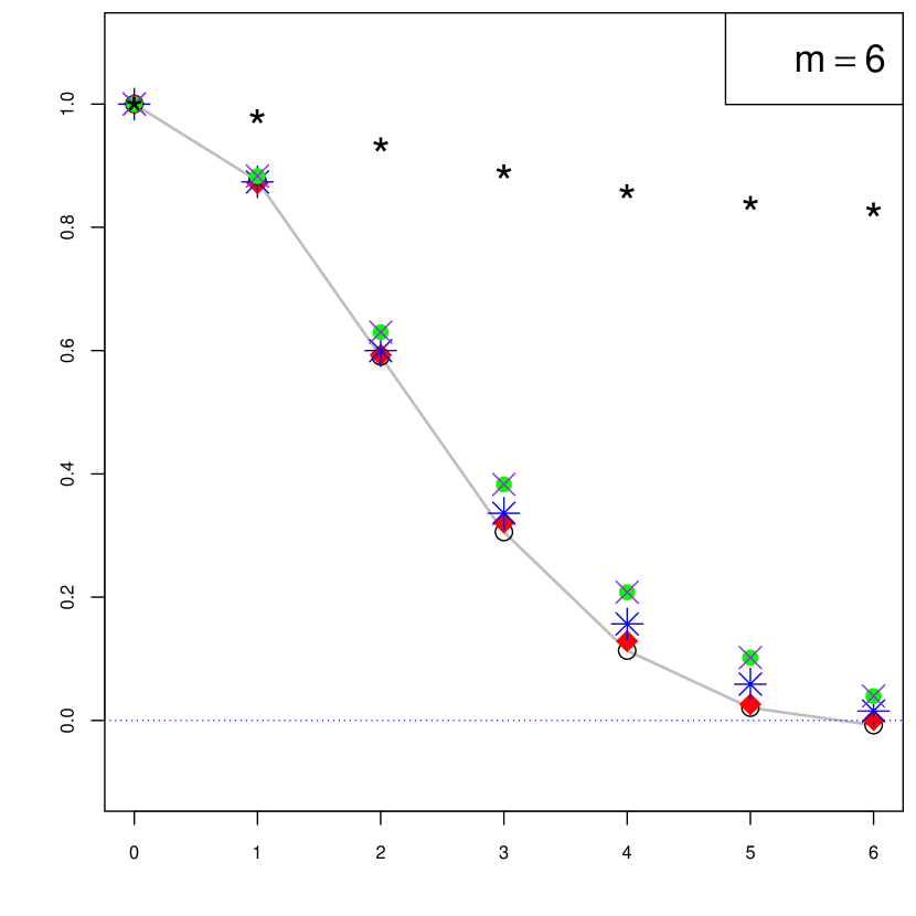
A

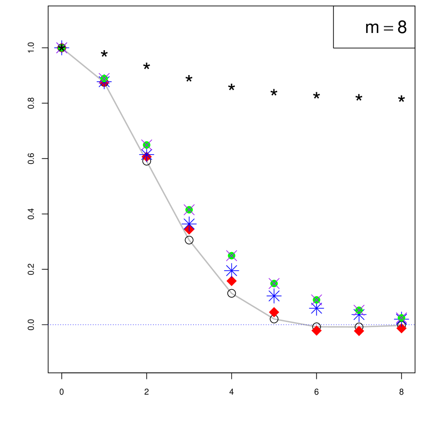
B

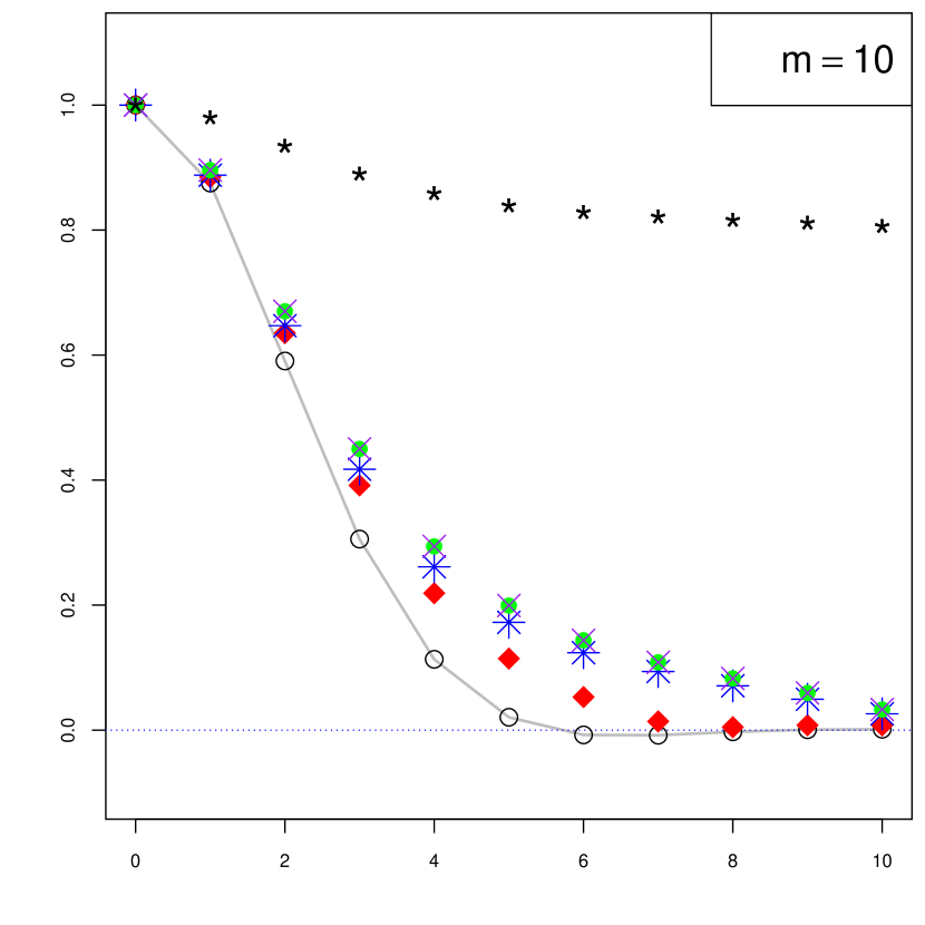
C

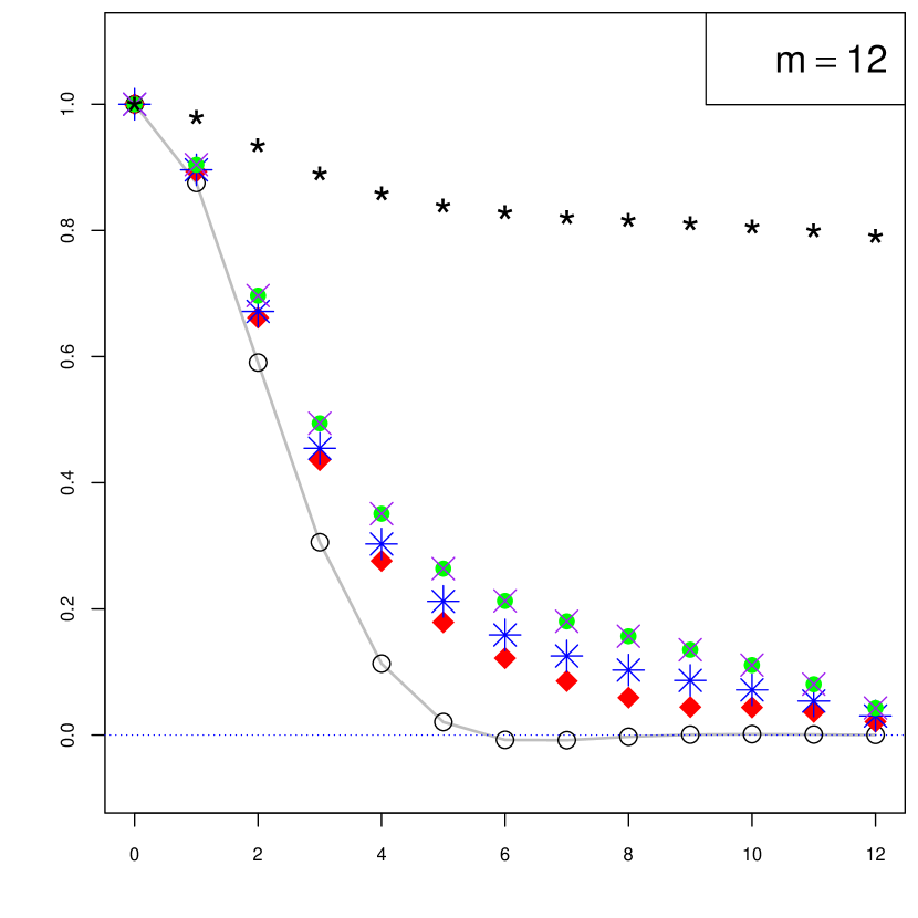
D

Figure 2. Correlation estimators from ion channel recordings shown in Figure 1A. true ($\circ$); $\widehat{\rho}_{O}$, optimized difference-based ($\blacklozenge$); $\widehat{\rho}_{H}$, Herrmann et al., (1992)’s (*); $\widehat{\rho}_{M}$, Müller and Stadtmüller, (1988)’s (•); $\widehat{\rho}_{R}$, adapted-Rice, (1984)’s ($\times$); $\widehat{\rho}_{HV}$, Hall and Van Keilegom, (2003)’s ($\star$).

The main goal of this section is to explore an application of our autocovariance estimation techniques in a changepoint problem. To this end, we introduce a method for JUmp Segmentation of (short-range) Depedent data ($\operatorname{JUSD}$). This method combines the multiscale changepoint estimator introduced by Frick et al., (2014) with the autocovariance estimates proposed in this paper.

7.2. Jump segmentation for dependent data

Now we briefly describe $\operatorname{JUSD}$. Let ${\bf Y}$ denote the vector of observations $y_{i}=f_{i}+\varepsilon_{i}$ following (1.1) and for simplicity suppose that the errors $\varepsilon_{i}$ are Gaussian distributed. The multiscale approach to detect a change-point given in Eqs. (3)-(4) of Frick et al., (2014) suggests to calculate all local likelihood ratio test (LRT) statistics $T_{i}^{j}({\bf Y},f_{\mathcal{H}})$, $1\leq i<j\leq n$, and to use the maximum over these statistics as the final test statistic, say $T_{n}$. Here $\mathcal{H}$ denotes the hypothesis that $f$ takes a fixed value on the interval $[i/n,j/n]$. Then, estimates and confidence regions for the change-points of $f$ can be derived from the distribution of $T_{n}$, which can e.g. be obtained via simulations, see Frick et al., (2014) for the independent case.

In the current situation of $m$-dependent errors, for each $i$ and $j$ the local LRT depends also on the inverse of the $(j-i+1)\times(j-i+1)$ covariance Toeplitz matrix, say $\Sigma_{j-i+1}$. In the worst case scenario, the dimension of such matrices is $n^{2}$ and in order to avoid the expensive calculation of $\Sigma_{j-i+1}^{-1}$ we propose a more tractable multiscale statistic. We re-weight the partial sums of the observations $y_{i}$ according to the dependency. More precisely, let $S_{i}^{j}=y_{i}+\cdots+y_{j}$, $i<j$, and consider the modified local statistics based on partial sums

$${\tilde{T}_{i}^{j}({\bf Y};f_{\mathcal{H}})}={|S_{i}^{j}-f_{\mathcal{H}}|^{2}}/{{\mathsf{VAR}(S_{i}^{j})}},\quad 1\leq i<j\leq n.$$

Now our proposal ($\operatorname{JUSD}$) consists of utilizing our difference-based estimates $\widehat{\gamma}_{O}$ to estimate ${\mathsf{VAR}(S_{i}^{j})}=(j-i+1)\,\gamma_{0}+2\sum_{k=1}^{m}(j-i+1-k)_{+}\,\gamma_{k}$, here $x_{+}=\max(0,x)$. The corresponding modified version of $T_{n}$ is denoted by $\tilde{T}_{n}$. Under the true error model, Monte Carlo simulations allow us then to determine the finite-sample distribution of $\tilde{T}_{n}$, and the subsequent estimation of the number of changepoints, locations and levels of $f$ is carried out as in Eqs.(5)-(6) of Frick et al., (2014).

For the simulation design of this section we use the signal introduced in Section 6.1 and a $6$-dependent Gaussian process for the error model. This error model corresponds to the estimated dependence structure of the ion channels introduced in Section 7.1, see Figure 2A. To simplify matters in the Monte Carlo experiment to determine the finite sample distribution of $\tilde{T}_{n}$, we will use an equivalent MA(6) representation for the error model. The coefficients of this MA(6) model are obtained via an application of the Durbin-Levinson algorithm (Proposition 5.2.1 of Brockwell and Davis, (2006)) to the sequence $\widehat{\gamma}_{h}^{(6)}(d_{h,6})$, $h=0,1,\ldots,6$, cf. (2.12)-(2.14).

This Monte Carlo experiment is performed only once and its output is used to assess the performance of $\operatorname{JUSD}$ in estimating the signal from 500 samples of size $n=1\,600$. For comparison, we have also utilized the R function smuceR which was designed for independent errors by Hotz and Sieling, (2015) to estimate changepoint locations and levels in the current simulation. In each simulation the significance level of the estimated number of change points was set to $\alpha=0.05$ in both methods. Figure 3A displays the fit of $\operatorname{JUSD}$ and $\operatorname{SMUCE}$ on one realization of the $y_{i}$’s and Figure 3B shows the same fits on a small part of this simulated dataset. Unlike $\operatorname{JUSD}$, $\operatorname{SMUCE}$ does not take into account the correlation between observations and this leads to a clear overestimation of the number of changepoints, see Figure 3C.

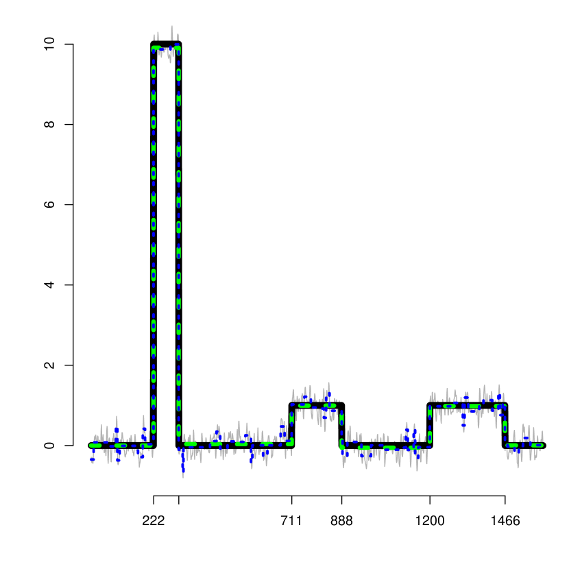
A

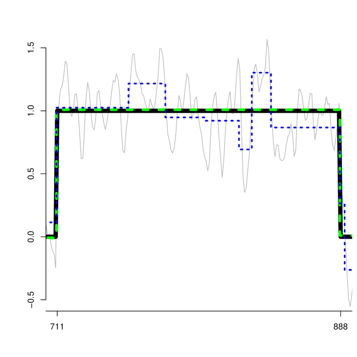
B

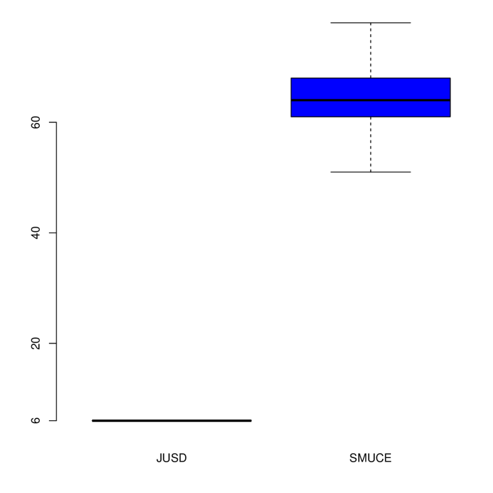
C

Figure 3. (A) (Gray background) An example of observations $y_{i}$’s as described in Section 7.2. ( ) True piecewise constant signal as described in Section 6.1. (     ) JUmp Segmentation for Dependent data as introduced in Section 7.2, (       ) Simultaneous MUltiscale Changepoint Estimator as presented by Frick et al., (2014). (B) Fit of JUSD and SMUCE on data shown in (A) restricted to the interval $[711,888)$. (C) Boxplot of estimated number of changepoints by $\operatorname{JUSD}$ and $\operatorname{SMUCE}$; true number of change-points is 6.

Supporting information for “Autocovariance estimation in regression with a discontinuous signal and $m$-dependent errors: A difference-based approach”

Appendix A Proofs and auxiliary results for Section 3

Throughout this supplementary materials we use the following notation: $n_{m}:=n-2(m+1)$, $n_{h}:=n-h$; $f_{i}$ denotes $f(x_{i})$, $v_{i:(i+h)}$ denotes the vector $(v_{i}\,v_{i+1}\,\cdots\,v_{i+h})^{\top}\in\mathbb{R}^{h+1}$ (we use this notation with $v\in\{y,f,\varepsilon\}$), $\langle\boldsymbol{a},\boldsymbol{b}\rangle$ denotes the inner product between the vectors $\boldsymbol{a}$ and $\boldsymbol{b}$, ${\bf 1}$ denotes the vector of ones, and for $x\in\mathbb{R}^{d}$, $\|x\|$ denotes its Euclidean norm.

A.1. Proofs for Section 3.1

We begin with some preliminary results. For $l<n$, let ${\bf Q}_{1}(Y,\boldsymbol{w}_{l})$ be a difference-based estimator of order $l$ and gap 1, cf. Eq. (2.2). With $\widetilde{D}$ as defined in (3.1) define the $(l+2)\times(l+2)$ matrix $D:=\widetilde{D}^{\top}\,\widetilde{D}$. Observe that the identity

$$\sum_{i=j}^{j+1}\,\left(d_{0}y_{i}+d_{1}y_{i+1}+\cdots+d_{l}\,y_{i+l}\right)^{2}=y_{j:(j+l+1)}^{\top}\,D\,y_{j:(j+l+1)},\quad j\leq n-2l-3,$$

implies that

$$2n_{l}\,P(\boldsymbol{w}_{l})\,{\bf Q}_{1}(Y,\boldsymbol{w}_{l})=\langle\boldsymbol{w}_{l},y_{1:(1+l)}\rangle^{2}+\sum_{j=1}^{n_{l}}y_{j:(j+l+1)}^{\top}\,D\,y_{j:(j+l+1)}+\langle\boldsymbol{w}_{l},y_{(n-l):n}\rangle^{2},$$ (A.1)

where $P(\boldsymbol{w}_{l})=\sum_{i=0}^{l}d_{i}^{2}$. In Eq. (A.1) it is not difficult to see that $\mathsf{E}[\langle\boldsymbol{w}_{l},y_{k:(k+l)}\rangle^{2}]=o(n)$ for $k=1,n-l$ and that for $j<n-l$, $\mathsf{E}[y_{j:(j+l+1)}^{\top}\,D\,y_{j:(j+l+1)}]=\|\widetilde{D}f_{j:(j+l+1)}\|^{2}+\mathsf{E}[\varepsilon_{j:(j+h+1)}^{\top}\,D\,\varepsilon_{j:(j+h+1)}]$. Next, we combine this with Proposition 1 and get that,

$$\mathsf{E}\left[P(\boldsymbol{w}_{l}){\bf Q}_{1}(Y,\boldsymbol{w}_{l})\right]=\boldsymbol{w}_{l}^{\top}\,\Sigma_{l+1}\,\boldsymbol{w}_{l}+\frac{1}{2n_{l}}\,\sum_{j=1}^{n_{l}}\,\|\widetilde{D}f_{j:(j+l+1)}\|^{2}+o(1),$$ (A.2)

where $\Sigma_{l+1}$ is the $(l+1)\times(l+1)$ autocovariance matrix $\Sigma_{l+1}=\left(\gamma_{|i-j|}\right)_{i,j=1,\ldots,l}.$

Proof of Theorem 5.

It suffices to consider the difference-based estimator of order $l<n$ and gap 1, ${\bf Q}_{1}(Y,\boldsymbol{w}_{l})$. For $l\leq m$, due to Lemma 1, (A.2) becomes

$$\mathsf{E}\left[P(\boldsymbol{w}_{l}){\bf Q}_{1}(Y,\boldsymbol{w}_{l})\right]=B_{l}+\mathcal{O}\left(n^{-1}\,J_{K}\,\sum_{k=1}^{l}\left(\sum_{j=k}^{l}\,d_{j}\right)^{2}\right),$$ (A.3)

where

$$~{}B_{l}=\boldsymbol{w}_{l}^{\top}\,\Sigma_{l+1}\,\boldsymbol{w}_{l}=\gamma_{0}(d_{0}^{2}+\cdots+d_{l}^{2})+2\gamma_{1}(d_{0}d_{1}+\cdots+d_{l-1}d_{l})+\cdots+2\gamma_{l}d_{0}d_{l}.$$ (A.4)

From now on in this proof we assume that $J_{K}=o(n)$ and disregard the second summand in the right-hand side of (A.3). Since constraint $\langle\boldsymbol{w}_{l},\boldsymbol{1}\rangle=0$ implies that at least one of the weights $d_{j}$ is nonzero, for simplicity from now on we assume that $d_{0}\neq 0$. According to Lemma 4 in this case there does not exist any constant $c$ such that $B_{l}=c\,\gamma_{0}$, that is, no difference-based estimate of the form ${\bf Q}_{1}(Y,\boldsymbol{w}_{l})$ can be an asymptotically unbiased estimate for $\gamma_{0}$ for $l\leq m$.

Next, suppose that $m<l\leq n$. In what follows, for simplicity, let us assume that $n=N(g+1)$ for some integer $N\geq 1$ and $g=m$. Observe that in this case Proposition 1 and (A.3) yield, $\mathsf{E}\left[p(\boldsymbol{w}_{l}){\bf Q}_{1}(Y,\boldsymbol{w}_{l})\right]=B_{l}+o(1)$. Due to $m$-dependency, the covariance matrix $\Sigma_{l+1}$ appearing in $B_{l}$ is an $(m+1)$-banded Toeplitz matrix, i.e., the $(i,j)$ entry of $\Sigma_{l+1}$ is given by $\gamma_{|j-i|}\neq 0$ if $|j-i|\leq m$, and outside the $(m+1)$-diagonal the entries of $\Sigma_{l+1}$ are equal to 0. Suppose that $\boldsymbol{w}_{l}$ has entries $d_{0}=1$ and $d_{j}\neq 0$, for $j=k(g+1)$ with $k=1,\ldots,N-1$, and $d_{j}=0$ otherwise. Clearly, $B_{l}=P(\boldsymbol{w}_{l})\,\gamma_{0}$. Now we show that any asymptotically unbiased estimate for $\gamma_{0}$ is necessarily of the form just described. Indeed, it suffices to consider the vector $\boldsymbol{w}_{l}^{\ast}$, whose entries are identical to those of $\boldsymbol{w}_{l}$ except for $d_{\kappa}\neq 0$ for some $\kappa\in\{1,\ldots,m\}$. In this case, due to the form of the covariance matrix $\Sigma_{l+1}$, $(\boldsymbol{w}_{l}^{\ast})^{\top}\,\Sigma_{l+1}\,\boldsymbol{w}_{l}^{\ast}=c_{1}\gamma_{0}+2\,d_{\kappa}\,\gamma_{\kappa}$, for some constant $c_{1}$. Since $\gamma_{\kappa}\neq 0$, no difference-based estimate of the form ${\bf Q}_{1}(Y,\boldsymbol{w}_{l}^{\ast})$ can be an asymptotically unbiased estimate for $\gamma_{0}$.

Note that the arguments above hold also for $g\geq m$. Thus, we have shown that for ${\bf Q}_{1}(Y,\boldsymbol{w}_{l})$ to be an (asymptotically unbiased) estimate for $\gamma_{0}$, the vector of weights $\boldsymbol{w}_{l}$ must have the form $\boldsymbol{w}_{l}=(\boldsymbol{v}_{0}\quad\boldsymbol{v}_{1}\quad\cdots\quad\boldsymbol{v}_{N-1})^{\top}$, where $\boldsymbol{v}_{i}=(d_{i\cdot g}\quad 0\quad\cdots\quad 0)^{\top}\in\mathbb{R}^{g+1}$, $i=0,\ldots,N-1$; $d_{0}\neq 0$, $d_{k\cdot g}\neq 0$ for some $1\leq k\leq N-1$, and $\sum_{i=0}^{N-1}d_{i\cdot g}=0$. This completes the proof. ∎

Lemma 4.

Suppose that the conditions of Theorem 5 hold. Let ${\bf Q}_{1}(Y,\boldsymbol{w}_{l})$ be the difference-based estimator of order $l<n$ and gap 1, cf. (2.2). Then for $l\leq m$, there does not exist any constant $c\neq 0$ such that $B_{l}=\boldsymbol{w}_{l}^{\top}\,\Sigma_{l+1}\,\boldsymbol{w}_{l}=c\,\gamma_{0}$, where $\Sigma_{l+1}$ is defined by (A.2).

Proof.

We use induction over $l$. For $l=1$, $B_{1}=\gamma_{0}(d_{0}^{2}+d_{1}^{2})+2\gamma_{1}d_{0}d_{1}$, cf. (A.4). Since by assumption $\gamma_{1}\neq 0$ (and $d_{0}\neq 0$), $d_{1}$ is necessarily equal to zero but this implies that $\gamma_{0}=0$ to fulfill (2.3). This contradiction shows that the claim holds for $h=1$. Then we assume that the claim holds for $l=k\leq m-1$. Let $\tilde{k}=k+1$ and now note that for $B_{\tilde{k}}=c\,\gamma_{0}$ to hold for some $c\neq 0$, necessarily $\gamma_{\tilde{k}}d_{0}d_{\tilde{k}}=0$. Since $\gamma_{\tilde{k}}\neq 0$ and $d_{0}\neq 0$, necessarily $d_{\tilde{k}}=0$. The latter shows that $B_{\tilde{k}}=B_{k}$. Hence, the claim holds for $l=k+1$ and this completes the proof. ∎

Proof of Lemma 1.

For $j<n-l$ define $s_{j,l}=\langle\boldsymbol{w}_{l},f_{j:(j+l)}\rangle^{2}$ and note that $\|\widetilde{D}f_{j:(j+l+1)}^{\top}\|^{2}=s_{j,l}+s_{j+1,l}$, see (3.1). In what follows we only consider $s_{j,l}$ since $s_{j+1,l}$ can be handled similarly.

Under the convention $t_{k}=\lfloor n\tau_{k}\rfloor$, $f(x_{i})=a_{k}$ if and only if $t_{k-1}\leq i<t_{k}$. Then

$$\sum_{j=1}^{n_{l}}s_{j,l}\leq\sum_{i=0}^{K-1}\left[\sum_{j=t_{i}}^{t_{i+1}-l-1}s_{j,l}+\sum_{j=t_{i+1}-l}^{t_{i+1}-1}s_{j,l}\right].$$ (A.5)

Then note that for any $i\in\{0,\ldots,K-1\}$,

$$\sum_{j=t_{i}}^{t_{i+1}-l-1}s_{j,l}=a_{i}^{2}\langle\boldsymbol{w}_{l},\boldsymbol{1}\rangle^{2}(t_{i+1}-t_{i}-l-1)$$

and utilizing that $d_{0}+\cdots+d_{l}=0$,

$$\sum_{j=t_{i+1}-l}^{t_{i+1}-1}s_{j,l}=\sum_{j=t_{i+1}-l}^{t_{i+1}-1}(d_{0}f_{j}+\cdots+d_{l}f_{j+l})^{2}\\ =(a_{i}-a_{i+1})^{2}\,\sum_{k=1}^{l}\left(\sum_{j=k}^{l}\,d_{j}\right)^{2}.$$

Substituting these expressions into (A.5) we obtain the right-hand side of (3.2). This completes the proof. ∎

Proposition 1.

For $l<n$, let $\boldsymbol{w}_{l}\in\mathbb{R}^{l+1}$ be the vector of weights in ${\bf Q}_{1}(Y,\boldsymbol{w}_{l})$, cf. (2.2). Let $D=\widetilde{D}^{\top}\,\widetilde{D}$ where $\widetilde{D}$ is defined by (3.1). Then

$$\mathsf{E}[\varepsilon_{j:(j+l+1)}^{\top}\,D\,\varepsilon_{j:(j+l+1)}]=2\,\boldsymbol{w}^{\top}_{l}\,\Sigma_{l+1}\,\boldsymbol{w}_{l}.$$

Proof.

Let $\Sigma_{l+1}$ be the matrix defined in (A.2) and note that

$$\mathsf{E}[\varepsilon_{j:(j+l+1)}^{\top}\,D\,\varepsilon_{j:(j+l+1)}]=\mbox{tr}\{D\Sigma_{l+2}\}=\mbox{tr}\{\widetilde{D}\,\Sigma_{l+2}\,\widetilde{D}^{\top}\}.$$

Then, observe that the $2\times 2$ matrix $\widetilde{D}\,\Sigma_{l+2}\,\widetilde{D}^{\top}$ can be written as:

$$\widetilde{D}\,\Sigma_{l+2}\,\widetilde{D}^{\top} =\begin{pmatrix}\boldsymbol{w}^{\top}_{l}\,\Sigma_{l+1}&\langle\boldsymbol{w}_{l},\gamma_{(l+1):1}\rangle\\ \langle\boldsymbol{w}_{l},\gamma_{(l+1):1}\rangle&\boldsymbol{w}^{\top}_{l}\,\Sigma_{l+1}\end{pmatrix}\,\begin{pmatrix}\boldsymbol{w}_{l}&0\\ 0&\boldsymbol{w}_{l}\end{pmatrix},$$

where $\gamma_{(l+1):1}:=(\gamma_{l+1}\quad\gamma_{l}\quad\cdots\quad\gamma_{2}\quad\gamma_{1})^{\top}\in\mathbb{R}^{l+1}$. A straightforward calculation yields, $\mbox{tr}\{\widetilde{D}\,\Sigma_{l+2}\,\widetilde{D}^{\top}\}=2\boldsymbol{w}^{\top}_{l}\,\Sigma_{l+1}\,\boldsymbol{w}_{l}$. ∎

A.2. Proofs for Section 3.2

We will assume that the conditions of Theorem 1 hold. Also we will use the following notation: $\chi_{h}(f_{i}):=f_{i}-f_{i+h}$, for $d\in\mathbb{R}$, $\delta_{i}(d):=s_{0}(i)+d\,s_{2(m+1)}(i)$ where for $k\geq 0$, $s_{k}(i):=f_{i+k}-f_{i+m+1}$, $\eta_{i}(d):=\varepsilon_{i}-\varepsilon_{i+m+1}+d(\varepsilon_{i+2(m+1)}-\varepsilon_{i+m+1})$, set $P(d)=2(d^{2}+d+1)$ and for given $\tau_{i},\tau_{j}\in[0,1]$, $1\leq L,R\leq n$,

$$I_{\tau_{i},\tau_{j}}^{L,R}:=[\tau_{i}-L/n,\tau_{j}-R/n).$$ (A.6)

Also, $I_{\tau_{i}}^{L,R}:=I_{\tau_{i},\tau_{i}}^{L,R}$. Under the convention $t_{j}=\lfloor n\tau_{j}\rfloor$, we will denote $I_{t_{i},t_{j}}^{L,R}:=[t_{i}-L,t_{j}-R)$ and use that $i/n\in I_{\tau_{i},\tau_{j}}^{L,R}$ if and only if $i\in I_{t_{i},t_{j}}^{L,R}$ without further mention.

The following identities are of great use in what follows: for any integers $r,s,u$ and $v$,

$$\mathsf{E}[\varepsilon_{r}^{2}\,\varepsilon_{s}^{2}] =\gamma_{0}^{2}+2\,\gamma_{|r-s|}^{2}$$ (A.7)

$$\mathsf{E}[\varepsilon_{r}^{2}\,\varepsilon_{u}\,\varepsilon_{v}] =\gamma_{0}\gamma_{|u-v|}+2\gamma_{|r-u|}\gamma_{|r-v|}$$ (A.8)

$$\mathsf{E}[\varepsilon_{r}\,\varepsilon_{s}\,\varepsilon_{u}\,\varepsilon_{v}] =\gamma_{|r-s|}\gamma_{|u-v|}+\gamma_{|r-u|}\gamma_{|s-v|}+\gamma_{|r-v|}\gamma_{|s-u|},$$ (A.9)

cf. Theorem 3.1 of Triantafyllopoulos, (2003).

Lemma 5.

Let $i\geq 1$, $l\geq 1$, $0\leq h\leq(m+1)$ and define $E_{i,l,h}=d_{0}\,\varepsilon_{i}+d_{1}\varepsilon_{i+h}+d_{2}\varepsilon_{i+2h}+\cdots+d_{l}\varepsilon_{i+lh}$. Then,

$$\mathsf{E}[E_{i,l,h}^{2}]=\gamma_{0}(d_{0}^{2}+d_{1}^{2}+d_{2}^{2}+\cdots+d_{l}^{2})+2\,\sum_{j=0}^{l-1}\sum_{k=j+1}^{l}\,d_{j}\,d_{k}\,\gamma_{|j-k|\,h}$$

Proof.

Write $E_{i,l,h}^{2}=A_{i,l,h}+2B_{i,l,h}$, where

$$A_{i,l,h}=\sum_{j=0}^{l}\,d_{j}^{2}\varepsilon_{i+jh}^{2},\quad B_{i,l,h}=\sum_{j=0}^{l-1}\,x_{j}(i,l,h),\quad x_{j}(i,l,h)=d_{j}\varepsilon_{i+jh}\,\,\sum_{k=j+1}^{l}\,d_{k}\,\varepsilon_{i+kh}.$$ (A.10)

The result follows by noticing that due to stationarity, for any integers $i$, $j$, $k$ and $h$, $\mathsf{E}[\varepsilon_{i+jh}^{2}]=\gamma_{0}$ and $\mathsf{E}[\varepsilon_{i+jh}\varepsilon_{i+kh}]=\gamma_{|j-k|h}$. ∎

Corollary 1.

For $l=2$, $d_{0}=1$, $d_{1}=-(d+1)$ and $d_{2}=d$, $\mathsf{E}[\eta_{i}^{2}(d)]=2(d^{2}+d+1)\,\gamma_{0}$.

Lemma 6.

For $i\geq 1$, $l\geq 1$, $\mathsf{E}[E^{4}_{i,l,m+1}]=3\,\gamma_{0}^{2}\,(d_{0}^{2}+d_{1}^{2}+\cdots+d_{l}^{2})^{2}$.

Proof.

From (A.10), $E^{4}_{i,l,m+1}=A^{2}_{i,l,m+1}+4A_{i,l,m+1}B_{i,l,m+1}+4B^{2}_{i,l,m+1}$. Note that (A.8) implies that $\mathsf{E}[A_{i,l,m+1}\,B_{i,l,m+1}]=0$. That is,

$$\mathsf{E}[E^{4}_{i,l,m+1}]=\mathsf{E}[A^{2}_{i,l,m+1}]+4\mathsf{E}[B^{2}_{i,l,m+1}].$$ (A.11)

Eq. (A.7) yields that for any integers $i$, $j$ and $k$, $\mathsf{E}[\varepsilon_{i+j(m+1)}]=3\gamma_{0}^{2}$ and $\mathsf{E}[\varepsilon_{i+j(m+1)}\,\varepsilon_{i+k(m+1)}]=\gamma_{0}^{2}$. Consequently,

$$~{}\mathsf{E}[A^{2}_{i,l,m+1}]=\gamma_{0}^{2}\left(3\sum_{j=0}^{l}\,d_{j}^{4}+2\sum_{k,j}\,d_{k}^{2}\,d_{j}^{2}\right).$$ (A.12)

Next, Eq. (A.9) implies that for $r\neq s$, $\mathsf{E}[x_{r}(i,l,m+1)x_{s}(i,l,m+1)]=0$, see (A.10) for definition of $x_{(\cdot)}(i,l,m+1)$. Hence,

$$~{}\mathsf{E}[B^{2}_{i,l,m+1}]=\sum_{j=0}^{l}\,\mathsf{E}[x_{j}^{2}(i,l,m+1)]=\gamma_{0}^{2}\sum_{k,j}\,d_{k}^{2}\,d_{j}^{2}.$$ (A.13)

The last equality follows from (A.7). The result follows by plugging A.12 and A.13 into A.11. ∎

Lemma 7.

Suppose that the conditions of Theorem 1 hold. Then,

$$\frac{\bf A}{8} :=\sum_{i=1}^{n_{m}-1}\sum_{j=i+1}^{n_{m}}\delta_{i}(d)\delta_{j}(d)\mathsf{E}[\eta_{i}(d)\eta_{j}(d)]=\left[-d(d+1)^{2}(m+1)+\sum_{h=1}^{m}\,q_{h}^{(m)}(d)\rho_{h}\right]\gamma_{0}\,J_{K},~{}$$ (A.14)

where $q_{h}^{(m)}(d)=[2(m+1)-3h](d^{4}+1)+d^{2}h$ and $\rho_{h}=\gamma_{h}/\gamma_{0}$.

Proof.

For $d\in\mathbb{R}$, let $S_{r}(d)=\sum_{i=1}^{n_{m}-r}\,\delta_{i}(d)\delta_{i+r}(d)$, $1\leq r<n_{m}$. First observe that due to stationarity, for any $i\geq 1$ and $h\geq 1$, $\Psi(h,d):=\mathsf{E}[\eta_{i}(d)\,\eta_{i+h}(d)]=2\,(d^{2}+d+1)\gamma_{h}-(d+1)^{2}\gamma_{|h-(m+1)|}+d\gamma_{|h-2(m+1)|}$. Then due to $m$-dependency, $\Psi(h,d)=0$ for all $h>3m+2$. Consequently, we can write

$$\frac{\bf A}{8}=\sum_{r=1}^{3m+2}\,\Psi(r)\,S_{r}.$$ (A.15)

Next, we present the details on how to compute $S_{0}(d)$. Utilizing (2.8) and (A.6), we can show that for given $\tau_{j}$,

$$\sum_{x_{i}\in I_{\tau_{j}}^{2(m+1),m+1}}\,\delta_{i}^{2}(d)=(m+1)d^{2}(a_{j+1}-a_{j})^{2},\quad\sum_{x_{i}\in I_{\tau_{j}}^{m+1,0}}\,\delta_{i}^{2}(d)=(m+1)(a_{j+1}-a_{j})^{2}.$$

Observe that $S_{0}(d)=\sum_{j=0}^{K-1}\,\sum_{x_{i}\in I_{\tau_{j}}^{2(m+1),m+1}\cup I_{\tau_{j}}^{m+1,0}}\,\delta_{i}^{2}(d)=(m+1)(d^{2}+1)\,J_{K}$. The key part in obtaining the summation $S_{r}(d)$, $r\geq 1$, consists of splitting it as shown above (and using (2.8)-(A.6)). Thus, we can show that $S_{r}(d)=T_{r}(d)\,J_{K}$ where

$$T_{r}(d)=\begin{cases}(m+1-r)d^{2}+rd+(m+1-r)&\mbox{ for }r=0,\ldots,m\\ d\,(2(m+1)-r)&\mbox{ for }r=m+1,\ldots,2m+1\\ 0&\mbox{ for }r\geq 2(m+1)\end{cases}.$$ (A.16)

In order to get (A.14), substitute (A.16) into (A.15) and arrange terms. This completes the proof. ∎

Lemma 8.

Suppose that the conditions of Theorem 1 hold. Then

$${\bf B} :=2\sum_{i=1}^{n_{m}-1}\sum_{j=i+1}^{n_{m}}\mathsf{E}[\eta_{i}^{2}(d)\,\eta_{j}^{2}(d)]=8n_{m}^{2}\,(d^{2}+d+1)^{2}\gamma_{0}^{2}+2\,\sum_{r=1}^{3m+2}(n_{m}-r)\,\Lambda_{r}(d)\geq 0.$$ (A.17)

where

$$\Lambda_{r}(d;\gamma_{(\cdot)}) =8\,(d^{2}+d+1)^{2}\gamma_{h}^{2}+2(1+d)^{4}\gamma_{|h-(m+1)|}^{2}+2d^{2}\gamma_{|h-2(m+1)|}^{2}$$

$$-4(1+d)[(1+d)^{3}+(d^{3}+d^{2}+d+1)]\gamma_{h}\,\gamma_{|h-(m+1)|}$$

$$-4d(d+1)^{2}\gamma_{|h-(m+1)|}\,\gamma_{|h-2(m+1)|}.$$ (A.18)

Proof.

Straightforward calculations and Eqs. (A.7), (A.8) and (A.9) yield that for $i\geq 1$ and $r\geq 0$,

$$\mathsf{E}[\eta_{i}^{2}(d)\,\eta_{i+r}^{2}(d)]=4\,(d^{2}+d+1)^{2}\gamma_{0}^{2}+\Lambda_{r}(d).$$

Arrange terms and use $m$-dependency to get

$$\frac{\bf B}{2}=\sum_{r=1}^{n_{m}-1}\,\sum_{s=1}^{n_{m}-r}\mathsf{E}[\eta_{s}^{2}(d)\,\eta_{s+r}^{2}(d)].$$

The result now follows by noticing that $\Lambda_{r}(d)=0$ for all $r\geq 3(m+1)$. ∎

Lemma 9.

Suppose that the assumptions of Theorem 1 hold. Additionally, assume that the correlation function $\rho_{h}=\gamma_{h}/\gamma_{0}$ satisfies that $\rho_{h}=\rho\in(\max\{\,-1,-8/(3m^{2})\,\},1)$, $1\leq h\leq m$. Then $p_{1}(d;\gamma_{(\cdot)})$ and $\mathsf{BIAS}^{\ast}[\widehat{\gamma}_{0}^{(m)}(d)]$ are minimized at $d=1$.

Proof.

Since $\mathsf{BIAS}[\widehat{\gamma}_{0}^{(m)}(d)]$ is minimized at $d=1$, cf. Theorem 2, we only need to focus on minimizing $p_{1}(\cdot;\gamma_{(\cdot)})$. Let $Q(d)=d^{2}+d+1$. It is easily seen that

$$p_{1}(d;\gamma_{(\cdot)})=\frac{m+1}{Q^{2}(d)}\left[2(d^{4}+1)+m(d^{4}+d^{2}+1)\sum_{h=1}^{m}\rho_{h}\right].$$

For $\rho=0$ (indepent observations) the result follows since $\operatorname*{argmin}_{d\in\mathbb{R}}(d^{4}+1)/Q^{2}(d)=1$. For $\rho>0$, we have that $\operatorname*{argmin}_{d\in\mathbb{R}}(d^{4}+d^{2}+1)/Q^{2}(d)=1$ and hence for $d\in\mathbb{R}$, $p_{1}(d;\gamma_{(\cdot)})\geq p_{1}(1;\gamma_{(\cdot)})$. For $\rho<0$, note that

$$\frac{\partial}{\partial d}\,p_{1}(d;\gamma_{(\cdot)})=\frac{2(m+1)(d^{2}-1)(d^{2}(\rho\,m^{2}+2)+d(\rho\,m^{2}+4)+\rho\,m^{2}+2)}{Q(d)^{3}},$$

It is immediate that on $\mathbb{R}$, the critical points of $p_{1}$ are -1 and 1. For $\rho\in(-8/(3m^{2}),0)$, $\frac{\partial^{2}}{\partial d^{2}}\,p_{1}(-1;\gamma_{(\cdot)})=-4\rho\,m^{2}>0$ and $\frac{\partial^{2}}{\partial d^{2}}\,p_{1}(d;\gamma_{(\cdot)})=4(9\rho\,m^{2}+24)/81>0$, i.e., both critical points are minima. The result follows by noting that $p_{1}(1;\rho)=p_{1}(-1;\rho)/9$. ∎

The following auxiliary results are used in the proof of Theorem 1. Recall that $\widehat{\delta}^{(h)}$ is the ordinary difference-based estimator of gap $h$, cf. (2.4). Define

$$~{}{\bf C}_{h}^{1/2}=\sum_{i=1}^{n-h}(\varepsilon_{i}-\varepsilon_{i+h})^{2},\quad{\bf D}_{h}^{1/2}=\sum_{i=0}^{K-1}\sum_{j\in I_{t_{i}}^{h,0}}\,(a_{i}-a_{i+1})(\varepsilon_{j}-\varepsilon_{j+h}).$$ (A.19)

We can show that

$$(2(n-h))^{2}\,\mathsf{E}[(\widehat{\delta}^{(h)})^{2}]=h^{2}J_{K}^{2}+4hJ_{K}(n-h)(\gamma_{0}-\gamma_{h})+\mathsf{E}[{\bf C}_{h}]+\mathsf{E}[{\bf D}_{h}].$$ (A.20)

For $\mathsf{E}[{\bf C}_{h}]$ observe that due to Eqs. (A.7)-(A.8)-(A.9),

$$\mathsf{E}[(\varepsilon_{i}-\varepsilon_{i+h})^{2}\,(\varepsilon_{j}-\varepsilon_{j+h})^{2}]=4(\gamma_{0}-\gamma_{h})^{2}+\vartheta_{1}(i,j)+\vartheta_{2}(i,j)$$

with

$$\vartheta_{1}(i,j)=\mbox{const.}\,\gamma_{|j-i+s|}^{2},\quad\vartheta_{2}(i,j)=\sum_{s,t}\,\mbox{const.}\,\gamma_{|j-i+s|}\gamma_{|j-i+t|},$$

where $s,t\in\{0,\pm h\}$. That is,

$$\mathsf{E}[{\bf C}_{h}]=[2(n-h)]^{2}(\gamma_{0}-\gamma_{h})^{2}+S_{1,n}^{(h)},$$ (A.21)

where $S_{1,n}^{(h)}=\sum_{i,j}^{n-2h}[\vartheta_{1}(i,j)+\vartheta_{2}(i,j)]$; note that $S_{1,n}^{(h)}=\mathcal{O}(n)$.

Lemma 10.

Suppose that the conditions of Theorem 1 hold. Let ${\bf D}_{h}$ be defined by (A.19). Then, $\mathsf{E}[{\bf D}_{h}]=F_{h}(\gamma_{(\cdot)})\,J_{K}$ where $F_{1}=2(\gamma_{0}-\gamma_{1})$ and for $2\leq h\leq m$

$$F_{h}(\gamma_{(\cdot)})=2\left[(h-1)(\gamma_{0}-\gamma_{h})+\sum_{j=2}^{h}\,\sum_{i=1}^{j+1}\left(2\gamma_{|j-i|}-\gamma_{|j-i-h|}-\gamma_{|j-i+h|}\right)\right]$$ (A.22)

Proof.

For $h=1$ the result follows by noting that for any $t_{i}$, $I_{t_{i}}^{h,0}=\{\,t_{i}-1\,\}$. For $2\leq h\leq m$ note that

$${\bf D}_{h}=\sum_{i=0}^{K-1}\sum_{k\in I_{t_{i}}^{h,0}}(a_{i}-a_{i+1})^{2}(\varepsilon_{k}-\varepsilon_{k+h})^{2}+\sum_{s=1}^{K-2}\sum_{r=1}^{K-1}(a_{s}-a_{s+1})(a_{r}-a_{r+1})(\tilde{{\bf D}}_{r,s}+\tilde{{\bf D}}_{s,r}),$$

where

$$\tilde{{\bf D}}_{s,t}=\sum_{i\in I_{t_{r}}^{h,0}}\sum_{j\in I_{t_{s}}^{h,0}}(\varepsilon_{i}-\varepsilon_{i+h})(\varepsilon_{j}-\varepsilon_{j+h}).$$

Since for any $t_{i}$, $\mathsf{E}\left[\sum_{j\in I_{t_{i}}^{h,0}}(\varepsilon_{j}-\varepsilon_{j+h})\right]^{2}=2(h-1)(\gamma_{0}-\gamma_{h})+\Lambda^{\ast}(h;\gamma_{(\cdot)})$, where

$$\Lambda^{\ast}(h;\gamma_{(\cdot)})=2\,\sum_{j=2}^{h}\,\sum_{i=1}^{j+1}\left(2\gamma_{|j-i|}-\gamma_{|j-i-h|}-\gamma_{|j-i+h|}\right),$$

the result is established if we show that $\mathsf{E}[\tilde{{\bf D}}_{r,s}]=\mathsf{E}[\tilde{{\bf D}}_{s,r}]=0$. To this end, observe that for any $s\in\{1,\ldots,K-2\}$ and $t\in\{s+1,\ldots,K-1\}$:

$$\mathsf{E}[\tilde{{\bf D}}_{s,r}] =\sum_{i=t_{s}-h}^{t_{s}-1}\sum_{i=t_{r}-h}^{t_{r}-1}\left[2\gamma_{|i-j|}-\gamma_{|j-i-h|}-\gamma_{|j-i+h|}\right]$$

let $$x=t_{r}-t_{s} \min_{1\leq i\leq K-1}|t_{i}-t_{i-1}|>4(m+1)$$ and recall that by assumption, to get,

$$=\sum_{i=1}^{h}\,\sum_{j=1}^{h}\,\left[2\gamma_{|x+j-i|}-\gamma_{|x+j-i-h|}-\gamma_{|x+j-i+h|}\right]=0.$$

The last equality follows because $\gamma_{|h|}=0$ for all $h\geq m+1$. A similar argument shows that $\mathsf{E}[\tilde{{\bf D}}_{r,s}]=0$. This completes the proof. ∎

From now on, $\sum_{i,j}:=\sum_{i=1}^{n_{m}}\sum_{j=1}^{n_{h}}$.

Lemma 11.

Supppose that the conditions of Theorem 1 hold. Let $\widehat{\delta}^{(h)}$ and $\widehat{\gamma}_{0}^{(m)}(d)$ be given by Eqs. (2.4)-(2.5). Then,

$$\mathsf{E}[\widehat{\gamma}_{0}^{(m)}(d)\times\widehat{\delta}^{(h)}]=\frac{1}{2P(d)n_{h}n_{m}}\left\{[I^{\ast}+II^{\ast}+III^{\ast}]\,J_{K}+S_{2,n}^{(h)}(d)\right\},$$ (A.23)

where

$$I^{\ast} =(m+1)(d^{2}+1)\,[2n_{h}(\gamma_{0}-\gamma_{h})+h\,J_{K}]$$

$$II^{\ast} =8(d^{2}-1)V_{h},\qquad V_{h}=\sum_{s=0}^{m}\sum_{t=1}^{h}\,\gamma_{s+t}-\sum_{s=1}^{m+1}\sum_{t=1}^{h}\,\gamma_{|t-s|},\quad 1\leq h\leq m,$$

$$III^{\ast} =2P(d)\,h\,n_{m}\gamma_{0}.$$

Here, $S_{2,n}^{(h)}(d)=\mathcal{O}(n)$ and does not depend on $J_{K}$.

Proof.

By definition

$$\mathsf{E}[\widehat{\gamma}_{0}^{(m)}(d)\times\widehat{\delta}^{(h)}]=\frac{\mathsf{E}[I+II+III]}{2P(d)\,n_{h}\,n_{m}},$$

where

$$I =\sum_{i,j}\left[\delta_{i}^{2}(d)(\chi_{j}+\varepsilon_{j}-\varepsilon_{j+h})^{2}\right],\quad II=2\sum_{i,j}\,\delta_{i}(d)\,\eta_{i}(d)\left[2\chi_{j}(\varepsilon_{j}-\varepsilon_{j+h})+(\varepsilon_{j}-\varepsilon_{j+h})^{2}\right]$$

$$III =\sum_{i,j}\eta_{i}^{2}(d)\left[\chi_{j}+\varepsilon_{j}-\varepsilon_{j+h}\right]^{2}$$

Since for all $j$, $\mathsf{E}[\varepsilon_{j}]=0$ and $\mathsf{E}[(\varepsilon_{j}-\varepsilon_{j+h})^{2}]=2(\gamma_{0}-\gamma_{h})$, we utilize the arguments leading to Eqs. (3.3)-(3.7) and get

$$I^{\ast}=\mathsf{E}[I]=(m+1)(d^{2}+1)\,[2n_{h}(\gamma_{0}-\gamma_{h})+h\,J_{K}]\,J_{K}.$$ (A.24)

Due to Gaussianity for any $i$ and $j$, $\mathsf{E}[\eta_{i}(d)(\varepsilon_{j}-\varepsilon_{j+h})^{2}]=0$. Thus, according to Lemma 12

$$I^{\ast\ast}=\mathsf{E}[II]=4\sum_{i,j}\mathsf{E}[\delta_{i}(d)\,\eta_{i}(d)\,\chi_{j}(\varepsilon_{j}-\varepsilon_{j+h})]=8(d^{2}-1)\,J_{K}\,V_{h}.$$ (A.25)

Gaussianity and Lemma 5 yield, $\sum_{i,j}\mathsf{E}[\eta_{i}^{2}(d)\chi_{j}(\varepsilon_{j}-\varepsilon_{j+h})]=0$, and $\mathsf{E}[\eta_{i}^{2}(d)]=2P(d)\gamma_{0}$, respectively. Consequently,

$$I^{\ast\ast\ast}=\mathsf{E}[III]=2P(d)\gamma_{0}\,n_{m}\,h\,J_{K}+S_{2,n}^{(h)}(d),$$ (A.26)

where by stationarity, $S_{2,n}^{(h)}(d)=\sum_{i,j}\mathsf{E}[\eta_{i}^{2}(d)(\varepsilon_{j}-\varepsilon_{j+h})^{2}]=\mathcal{O}(n)$. In order to get Eq. (A.23) sum up Eqs. (A.24)-(A.25)-(A.26) and arrange terms. ∎

Lemma 12.

Suppose that the conditions of Theorem 1 hold. Let

$$\Psi_{K,d}=\sum_{i,j}\,\delta_{i}(d)\,\eta_{i}(d)\chi_{j}(\varepsilon_{j}-\varepsilon_{j+h}).$$

Then,

$$\mathsf{E}[\Psi_{K,d}]=2(d^{2}-1)J_{K}\,V_{h}.$$ (A.27)

See Lemma 11 for a definition of $V_{h}$.

Proof.

Set $c_{m}=2(m+1)$. Since for given $j$,

$$\sum_{i\in I_{t_{j}}^{c_{m},c_{m}/2}}\delta_{i}(d)\,\eta_{i}(d) =d\,(a_{j}-a_{j+1})\times\sum_{i\in I_{t_{j}}^{c_{m},c_{m}/2}}\eta_{i}:={\bf E}_{\tau_{j}}(d),$$

$$\sum_{i\in I_{t_{j}}^{c_{m}/2,0}}\delta_{i}(d)\,\eta_{i}(d) =(a_{j}-a_{j+1})\times\sum_{i\in I_{t_{j}}^{c_{m}/2,0}}\eta_{i}(d):={\bf F}_{\tau_{j}}(d),$$

it follows that $\sum_{i}\,\delta_{i}(d)\eta_{i}(d)=\sum_{j}\,\left({\bf E}_{\tau_{j}}(d)+{\bf F}_{\tau_{j}}(d)\right)$.

Let $\sum_{j,I_{\tau_{j}}^{L,R}}:=\sum_{j=0}^{K-1}\sum_{i\in I_{\tau_{j}}^{L,R}}$. Note that $\chi_{i}=(a_{j}-a_{j+1}){1\textnormal{l}}_{I_{\tau_{j}}^{h,0}}(i)$ and this, in turn, implies that $\sum_{i}\chi_{i}(\varepsilon_{i}-\varepsilon_{i+h})=\sum_{j,i}(a_{j}-a_{j+1})(\varepsilon_{i}-\varepsilon_{i+h}):={\bf G}_{h}$. Consequently,

$$\Psi_{K,d}=\sum_{j=0}^{K-1}\left({\bf E}_{\tau_{j}}(d)+{\bf F}_{\tau_{j}}(d)\right)\times{\bf G}_{h}=T_{1}+T_{2}+T_{3}+U_{1}+U_{2}+U_{3},$$

where

$$T_{1} =d\,\sum_{j,I_{t_{j}}^{(c_{m},m/2)}}\,(a_{j}-a_{j+1})\varepsilon_{i}\,{\bf G}_{h},\quad T_{2}=-d(1+d)\,\sum_{j,I_{t_{j}}^{(c_{m},m/2)}}\,(a_{j}-a_{j+1})\varepsilon_{i+c_{m}/2}\,{\bf G}_{h}$$

$$T_{3} =d^{2}\,\sum_{j,I_{t_{j}}^{(c_{m},m/2)}}\,(a_{j}-a_{j+1})\varepsilon_{i+c_{m}}\,{\bf G}_{h},\quad U_{1}=\sum_{j,I_{t_{j}}^{(m/2,0)}}\,(a_{j}-a_{j+1})\varepsilon_{i}\,{\bf G}_{h},$$

$$U_{2} =-(1+d)\,\sum_{j,I_{t_{j}}^{(m/2,0)}}\,(a_{j}-a_{j+1})\varepsilon_{i+c_{m}/2}\,{\bf G}_{h},\quad U_{3}=d\,\sum_{j,I_{t_{j}}^{(m/2,0)}}\,(a_{j}-a_{j+1})\varepsilon_{i+c_{m}}\,{\bf G}_{h}.$$

The result follows by computing the expected value of $T$’s and $U$’s. Now we compute $\mathsf{E}[T_{1}]$ and $\mathsf{E}[U_{1}]$, the remaining terms of $\mathsf{E}[\Psi_{K,d}]$ can be treated similarly. In what follows,

$$\sum_{r,s}\,\mathscr{S}_{i,j}^{L_{1},R_{1},L_{2},R_{2}}:=\sum_{r\in I_{t_{i}}^{L_{1},R_{1}}}\,\sum_{s\in I_{t_{j}}^{L_{2},R_{2}}}\,\varepsilon_{r}(\varepsilon_{s}+\varepsilon_{s+h}).$$

We begin by writing $\mathsf{E}[T_{1}]=d\mathsf{E}[T_{1,1}+T_{1,2}]$, where $T_{1,1}=\sum_{j=0}^{K-1}(a_{j}-a_{j+1})^{2}\,\sum_{r,s}\,\mathscr{S}_{j,j}^{c_{m},c_{m}/2,h,0}$ and $T_{1,2}=\sum_{i=0}^{K-2}\,\sum_{j=i+1}^{K-1}(a_{i}-a_{i+1})\,(a_{j}-a_{j+1})\left(\sum_{r,s}\,\mathscr{S}_{i,j}^{c_{m},c_{m}/2,h,0}+\sum_{r,s}\,\mathscr{S}_{j,i}^{c_{m},c_{m}/2,h,0}\right)$. Note now that for any $\tau_{j}$ and due to $m$-dependency,

$$\mathsf{E}\left[\sum_{r,s}\mathscr{S}_{j,j}^{c_{m},c_{m}/2,h,0}\right]=\sum_{r=\tau_{j}-c_{m}}^{\tau_{j}-(m+2)}\sum_{s=\tau_{j}-h}^{\tau_{j}-1}[\gamma_{|r-s|}-\gamma_{|r-(s+h)|}]=\sum_{s=m+2}^{2(m+1)}\sum_{t=1}^{h}\gamma_{|s-t|}=\sum_{s=m+1}^{m+h}\sum_{t=1}^{h}\gamma_{|s-t|},$$ (A.28)

These calculations hold independently of the value of $\tau_{j}$, and consequently we get that $\mathsf{E}[T_{1,1}]=\sum_{r=m+1}^{m+h}\sum_{s=1}^{h}\gamma_{|r-s|}\,J_{K}$. Similar calculations along with the $m$-dependency and (2.8) allows us to get that $\mathsf{E}[T_{1,2}]=0$. All in all, we have shown that

$$\mathsf{E}[T_{1}]=d\,\sum_{s=m+1}^{m+h}\sum_{t=1}^{h}\,\gamma_{|h-(s+t)|}\,J_{K}.$$ (A.29)

Similar arguments yield,

$$\mathsf{E}[T_{2}] =-d(1+d)\sum_{s=1}^{m+1}\sum_{t=1}^{h}\,[\gamma_{|t-s|}-\gamma_{|t-(s+h)|}]\,J_{K}$$ (A.30)

$$\mathsf{E}[T_{3}] =d^{2}\,\sum_{s=0}^{m}\sum_{t=1}^{h}\,[\gamma_{s+t}-\gamma_{|h-(s+t)|}]\,J_{K}.$$ (A.31)

Now, we consider $\mathsf{E}[U_{1}]$. Write $U_{1}=U_{1,1}+U_{1,2}$, where

$$U_{1,1} =\sum_{j=0}^{K-1}(a_{j}-a_{j+1})^{2}\sum_{r,s}\,\mathscr{S}_{j,j}^{c_{m}/2,0,h,0}$$

$$U_{1,2} =\sum_{i=0}^{K-2}\,\sum_{j=i+1}^{K-1}(a_{i}-a_{i+1})\,(a_{j}-a_{j+1})\left(\sum_{r,s}\mathscr{S}_{i,j}^{c_{m}/2,0,h,0}+\sum_{r,s}\mathscr{S}_{j,i}^{h,0,c_{m}/2,0}\right)$$

Following (A.28) we can show that for any $\tau_{j}$, $\mathsf{E}\left[\sum_{r,s}\mathscr{S}_{j,j}^{c_{m}/2,0,h,0}\right]=\sum_{s=1}^{m+1}\sum_{t=1}^{h}[\gamma_{|t-s|}-\gamma_{|h-(t+s)|}]$. Again $m$-dependency and (2.8) allow us to show that $\mathsf{E}[U_{1,2}]=0$. Therefore,

$$\mathsf{E}[U_{1}]=\sum_{r=1}^{m+1}\sum_{s=1}^{h}[\gamma_{|r-s|}-\gamma_{|s-(r+h)|}]\,J_{K}.$$ (A.32)

Similar arguments yield,

$$\mathsf{E}[U_{2}] =-(1+d)\sum_{r=0}^{m+1}\sum_{s=1}^{h}\,[\gamma_{r+s}-\gamma_{|h-(r+s)|}]\,J_{K}$$ (A.33)

$$\mathsf{E}[U_{3}] =-d\,\sum_{r=m+1}^{m+h}\sum_{s=1}^{h}\,\gamma_{|h-(r+s)|}\,J_{K}.$$ (A.34)

Since $\sum_{r=0}^{m}\sum_{s=1}^{h}\,\gamma_{|h-(r+s)|}=\sum_{r=1}^{m+1}\sum_{s=1}^{h}\,\gamma_{|s-r|}$, $\sum_{r=1}^{m+1}\sum_{s=1}^{h}\,\gamma_{|s-(r+h)|}=\sum_{r=0}^{m}\sum_{s=1}^{h}\,\gamma_{r+s}$, (A.27) follows after summing up (A.29)-(A.34). ∎

Appendix B Proofs and auxiliary results for Section 4

In this Appendix we will assume that the conditions of Theorem 7 hold and use the notation introduced at the beginning of Appendices A and A.2. Also throughout this section $c_{m}=2(m+1)$ and the symbols $\kappa_{1}$, $\kappa_{2}$, etc., will denote constants which do not depend on $n$. We will write $\sum_{i,j}$ to denote $\sum_{i=1}^{n_{m}-1}\,\sum_{i=j+1}^{n_{m}}$.

Lemma 13.

Suppose that the conditions of Theorem 7 hold. Then, for $h=0,\ldots,m$,

$$\mathsf{E}[\widehat{\gamma}_{h}^{(m)}(d_{h,m})]=\gamma_{h}+\mathcal{O}(S_{n}),\qquad S_{n}=\sum_{j=1}^{K_{n}}\,\frac{\vartheta_{j}^{2}}{n}+\sum_{j=1}^{K_{n}}\,n^{-2(\alpha_{j}+1/2)}.$$

Proof.

We begin with the case $h=0$. Since $\widehat{\gamma}_{0}^{(m)}(d)=(2(d^{2}+d+1)\,n_{m})^{-1}\sum_{i=1}^{n_{m}}(\delta_{i}(d)+\eta_{i}(d))^{2}$, see Appendix A.2 for definition of $\delta_{i}(d)$ and $\eta_{i}(d)$, and $\mathsf{E}[\eta_{i}^{2}(d)]=2(d^{2}+d+1)\gamma_{0}$, cf. Corollary 1, in order to analyze the asymptotic bias of $\widehat{\gamma}_{0}^{(m)}(d)$ it suffices to focus on $\sum_{i}\,\delta_{i}^{2}(d)$. To this end we write $\delta_{i}^{2}(d)=s_{0}^{2}(i)+2d\,s_{0}(i)\,s_{c_{m}}(i)+d^{2}\,s_{c_{m}}^{2}(i)$ and note that for given $i$ there exists a unique $\tau_{j}$ such that

$$s_{0}(i)=\begin{cases}t(i,j):=a_{j}(i/n)-a_{j}((i+m+1)/n)&\mbox{ for }i\in I_{\tau_{j-1},\tau_{j}}^{(0,c_{m}/2)}\\ u(i,j):=a_{j}(i/n)-a_{j+1}((i+m+1)/n)&\mbox{ for }i\in I_{\tau_{j}}^{(c_{m}/2,0)}\\ \end{cases},$$

and a similar characterization holds for $s_{c_{m}}(\cdot)$, see Eq. (A.6) in Appendix A.2 for definition of $I_{\tau_{j-1},\tau_{j}}^{(0,c_{m}/2)}$ and $I_{\tau_{j}}^{(c_{m}/2,0)}$. This implies that the dominat terms in $\delta_{i}^{2}(d)$ are of the form $t^{2}(i,j)+u^{2}(i,j)$ and in what follows we provide bounds for these terms.

Recall that $\vartheta_{j}=a_{j}(\tau_{j+1}^{-})-a_{j+1}(\tau_{j+1})$ and by assumption there exists a number $c>0$ such that $|\vartheta_{j}|>c$ for all $j$. Utilizing the Hölder condition of $f$ we get

$$~{}\sum_{j=1}^{K_{n}-1}\,\sum_{i\in I_{\tau_{j-1},\tau_{j}}^{(0,c_{m}/2)}}\,t^{2}(i,j)\leq\kappa_{1,m}\,\sum_{j=1}^{K_{n}-1}\,n^{-2\alpha_{j}},$$ (B.1)

as well as

$$\sum_{j=1}^{K_{n}-1}\,\sum_{i\in I_{\tau_{j}}^{(c_{m}/2,0)}}\,u^{2}(i,j) \leq\sum_{j=1}^{K_{n}}\vartheta_{j}^{2}+\kappa_{2,m}\sum_{j=1}^{K_{n}}\,n^{-\alpha_{j}}\,\vartheta_{j}+\kappa_{1,m}\,\sum_{j=1}^{K_{n}}\,n^{-2\alpha_{j}}.$$

Here $\kappa_{1,m}=\sup_{j}\,(m+1)^{\alpha_{j}}<\infty$, $\kappa_{2,m}=2\,\kappa_{1,m}$. Define the set of indices $I_{K_{n}}:=\{j\in\{1,\ldots,K_{n}\}:|\vartheta_{j}|\geq 1\}$ and observe that

$$~{}\big{|}\sum_{j=1}^{K_{n}}n^{-\alpha_{j}}\,\vartheta_{j}\big{|}\leq\{\sum_{j\in I_{K_{n}}}\vartheta_{j}^{2}+\sum_{j\notin I_{K_{n}}}\,|\vartheta_{j}|\}\leq\{\sum_{j\in I_{K_{n}}}\vartheta_{j}^{2}+\sum_{j\notin I_{K_{n}}}\frac{1}{c}\,\vartheta_{j}^{2}\}\leq(1+c^{-1})\,\sum_{j=1}^{K_{n}}\,\vartheta_{j}^{2}.$$ (B.2)

From (B.1) and (B.2) follows that $\sum_{i=1}^{n_{m}}\delta_{i}^{2}(d)=\mathcal{O}\left(\sum_{j=1}^{K_{n}}\,{\vartheta_{j}^{2}}+\sum_{j=1}^{K_{n}}\,n^{-2\alpha_{j}}\right)$. Consequently,

$$\mathsf{E}[\widehat{\gamma}_{0}^{(m)}(d)]=\gamma_{0}+\mathcal{O}\left(S_{n}\right),\quad S_{n}=\sum_{j=1}^{K_{n}}\frac{\vartheta_{j}^{2}}{n}+\sum_{j=1}^{K_{n}}\,n^{-2(\alpha_{j}+1/2)}.$$ (B.3)

For $h\geq 1$, firstly note that by writing $\widehat{\delta}^{(h)}=(2(n-h))^{-1}\sum_{i=1}^{n_{h}}(s_{0}(i)+\eta_{i}(0))^{2}$ we can mimick the calculations above and get

$$\mathsf{E}[\widehat{\delta}^{(h)}]=\gamma_{0}-\gamma_{h}+\mathcal{O}(S_{n}).~{}$$ (B.4)

Then, by definition, $\widehat{\gamma}_{h}^{(m)}(d)=\widehat{\gamma}_{0}^{(m)}(d)-\widehat{\delta}^{(h)}$, cf. (2.6) in the Introduction, and the result follows by adding Eqs. (B.3) and (B.4). ∎

Lemma 14.

Suppose that the assumptions of Lemma 13 hold. Then

$$\mathsf{VAR}(\widehat{\gamma}_{0}^{(m)}(d))=\mathcal{O}(\sum_{j=1}^{K_{n}}(\vartheta_{j}^{2}/n^{2}+n^{-(\alpha_{j}+2)}))+\mathcal{O}(n^{-1})$$ (B.5)

the same result holds for $\mathsf{VAR}(\widehat{\delta}^{(h)})$. Moreover,

$$\mathsf{VAR}(\widehat{\gamma}_{h}^{(m)}(d))=\mathcal{O}(\mathsf{VAR}(\widehat{\gamma}_{0}^{(m)}(d))+(\sum_{j=1}^{K_{n}}\,{|\vartheta_{j}|}/{n})^{2}+(\sum_{j=1}^{K_{n}}\,n^{-(\alpha_{j}+1)})^{2}).$$ (B.6)

Proof.

We write $\widehat{\gamma}_{0}^{(m)}(d)=n^{-1}\sum\,b_{i}^{2}(d)$, where $b_{i}(d)=\delta_{i}(d)+\eta_{i}(d)$, see Appendix A.2 for notation. It is easily seen that $\mathsf{VAR}(b_{i}^{2}(d))=4\delta_{i}^{2}(d)\,\mathsf{VAR}(\eta_{i}(d))+\mathsf{VAR}(\eta_{i}^{2}(d))$. From Corollary 1 and Lemma 6, $\mathsf{VAR}(\eta_{i}(d))$ and $\mathsf{VAR}(\eta_{i}^{2}(d))$ are uniformly bounded. This implies that the order of magnitude of $\sum_{i}\,\mathsf{VAR}(b_{i}^{2}(d))$ depends solely on $\sum_{i}\,\delta_{i}^{2}(d)$. From arguments in the proof of Lemma 13 we get that

$$~{}\sum_{i=1}^{n_{m}}\,\mathsf{VAR}(b_{i}^{2}(d))=\mathcal{O}\left(\sum_{j=1}^{K_{n}}\vartheta_{j}^{2}+\sum_{j=1}^{K_{n}}\,n^{-2\alpha_{j}}\right)+\mathcal{O}(n).$$ (B.7)

It can be shown that $\mathsf{COV}(b_{i}^{2}(d),b_{j}^{2}(d))=4\delta_{i}(d)\delta_{j}(d)\mathsf{E}[\eta_{i}(d)\,\eta_{j}(d)]+2\delta_{i}(d)\mathsf{E}[\eta_{i}(d)\,\eta_{j}^{2}(d)]+2\delta_{j}(d)\mathsf{E}[\eta_{j}(d)\,\eta_{i}^{2}(d)]+\mathsf{COV}(\eta_{i}^{2}(d),\eta_{j}^{2}(d))$. Due to $m$-dependency and stationarity of moments up to 4-th order we get for any $i$ and $j$, $\mathsf{E}[\eta_{i}(d)\,\eta_{j}(d)]=\kappa_{2}\,\mu_{2}(|j-i|)$, $\mathsf{E}[\eta_{i}(d)\,\eta_{j}^{2}(d)]=\kappa_{3}\,\mu_{3}(|j-i|)$ and $\mathsf{COV}(\eta_{i}^{2}(d),\eta_{j}^{2}(d))=\kappa_{4}\,\mu_{4}(|j-i|)$, where $\mu_{2}(\cdot)$, $\mu_{3}(\cdot)$ and $\mu_{4}(\cdot)$ are functions which depend only on sums of moments of second, third and fourth order of $\varepsilon$, respectively. With the same arguments used in Lemma 7, we can establish that $\sum_{i,j}\,\delta_{i}(d)\,\delta_{j}(d)\mu_{2}(j-i)=\mathcal{O}(n)$. Similar arguments allow us to get that $\sum_{i,j}\delta_{i}(d)\,\mu_{3}(j-i)=\mathcal{O}(\sum_{i}\,\delta_{i}(d))$ and $\sum_{i,j}\,\mathsf{COV}(\eta_{i}^{2}(d),\eta_{j}^{2}(d))=\mathcal{O}(n)$.

All in all, we have proven that

$$~{}\sum_{i,j}\,\mathsf{COV}(b_{i}^{2}(d),b_{j}^{2}(d))=\mathcal{O}\left(\sum_{i}\,\delta_{i}(d)\right)+\mathcal{O}(n).$$ (B.8)

Since $\delta_{i}(d)=s_{0}(i)+ds_{c_{m}}(i)$, see Appendix A.2 for notation, from the characterization of $s_{0}(\cdot)$ and $s_{c_{m}}(\cdot)$ given in Lemma 13 it follows that the order of magnitude of (B.8) is driven by $\sum_{i}\,s_{0}(i)$. We get,

$$\bigg{|}\sum_{i=1}^{n_{m}}s_{0}(i)\bigg{|}=\bigg{|}\sum_{i=1}^{K_{n}-1}\left(\sum_{j\in I_{\tau_{i-1},\tau_{i}}^{(0,c_{m}/2)}}\,t(j,i)+\sum_{j\in I_{\tau_{i}}^{(c_{m}/2,0)}}\,u(j,i)\right)\bigg{|}=\mathcal{O}\left(\sum_{j=1}^{K_{n}}(n^{-\alpha_{j}}+|\vartheta_{j}|^{2})\right).$$ (B.9)

The latter follows because of Hölder condition on $f$ and calculations leading to (B.2). Observe that Eq. (B.5) follows by a combination of Eqs. (B.7)-(B.8)-(B.9).

For $h\geq 1$, we write $\widehat{\delta}^{(h)}=(2(n-h))^{-1}\sum_{i=1}^{n_{h}}(s_{0}(i)+\eta_{i}(0))^{2}$ and mimick the calculations above to deduce that $\widehat{\gamma}_{0}^{(m)}(d)$ and $\widehat{\delta}^{(h)}$ have variances of the same order. Then, since $\widehat{\gamma}_{h}^{(m)}=\widehat{\gamma}_{0}^{(m)}-\widehat{\delta}^{(h)}$, cf. (2.6) in the Introduction, we combine Eq. (B.5) and Lemma 15 below to show the validity of Eq. (B.6). This completes the proof. ∎

Lemma 15.

Suppose that the assumptions of Lemma 13 hold. Then

$$\mathsf{COV}(\widehat{\gamma}_{0}^{(m)}(d_{h,m}),\delta^{(h)})=\mathcal{O}\left((\sum_{j=1}^{K_{n}}\,{|\vartheta_{j}|}/{n})^{2}+(\sum_{j=1}^{K_{n}}\,n^{-(\alpha_{j}+1)})^{2}\right)+\mathcal{O}(n^{-1}).$$ (B.10)

Proof.

We begin with the case $d_{h,m}=1$. Throughout this proof $k\in\{h,c_{m}\}$. By definition,

$$\mathsf{COV}(\widehat{\gamma}_{0}^{(m)}(1),\widehat{\delta}^{(h)})=\frac{1}{12\,n_{m}\,n_{h}}\,\sum_{i=1}^{n_{m}}\,\sum_{j=1}^{n_{h}}\,\mathsf{COV}(z_{i,c_{m}},z_{j,h})+\mathcal{O}(n^{-1}),$$ (B.11)

where for given index $i$, $z_{i,k}=y_{i:(i+k+1)}^{\top}\,D_{k+2}\,y_{i:(i+k+1)}$, see Appendix A for notation of $y_{i:(i+k+1)}$ and Eq. (3.1) for definition of the $(k+2)\times(k+2)$ matrix $D_{k+2}$. We also write $c_{i}(k)=f_{i:(i+k+1)}^{\top}\,D_{k+2}\,\varepsilon_{i:(i+k+1)}$ and $d_{i}(k)=\varepsilon_{i:(i+k+1)}^{\top}\,D_{k+2}\,\varepsilon_{i:(i+k+1)}$ which by standard calculations yield $\mathsf{COV}(z_{i,c_{m}},z_{j,h})=4\mathsf{E}[c_{i}(c_{m})\,c_{j}(h)]+2\mathsf{E}[c_{i}(c_{m})\,d_{j}(h)]+2\mathsf{E}[c_{j}(h)\,d_{i}(c_{m})]-\mbox{tr}(D_{c_{m}+2}\,\Sigma_{c_{m}+2})\,\mbox{tr}(D_{h+2}\,\Sigma_{h+2})$. Stationarity and $m$-dependency, arguments also used in Lemma 14, allow us to get that the second, third and fourth summands above are sums of stationary moments of second, third and fourth order, respectively. Hence the contribution of these terms to (B.11) is of order $\mathcal{O}(n^{-1})$. It is not difficult to see that for given indeces $i$ and $j$, $c_{i}(m)\,c_{j}(h)$ is the sum of 8 terms of the form $(f_{i}-f_{i+(m+1)})(f_{j}-f_{j+h})(\varepsilon_{i}-2\varepsilon_{i+m+1}+\varepsilon_{i+2(m+1)})(\varepsilon_{j}-\varepsilon_{j+h})$ and due to stationarity and $m$-dependency, $\mathsf{E}[c_{i}(m)\,c_{j}(h)]$ is bounded by $|f_{i}-f_{i+(m+1)})(f_{j}-f_{j+h})|$. Now, since $s_{k}(i)=f_{i+k}-f_{i+m+1}$, see notation in Appendix A.2, we utilize the ideas leading to the bound of $\mathsf{VAR}(\widehat{\gamma}_{0}^{(m)}(1))$, cf. (B.5), and obtain that

$$\big{|}\sum_{i=1}^{n_{m}}\,\sum_{j=1}^{n_{h}}\,(f_{i}-f_{i+(m+1)})(f_{j}-f_{j+h})\big{|}=\mathcal{O}\left((\sum_{j=1}^{K_{n}}|\vartheta_{j}|)^{2}+(\sum_{j=1}^{K_{n}}\,n^{-\alpha_{j}})^{2}\right).$$ (B.12)

Thus for $d_{h,m}=1$, the result follows by a combination of Eqs. (B.11) and (B.12). For the other values of $d_{h,m}$, cf. (2.14) in the Introduction, we mimick the calculations above to complete the proof. ∎

References

• Bardet et al., (2012) Bardet, J.-M., Kengne, W., Wintenberger, O., et al. (2012). Multiple breaks detection in general causal time series using penalized quasi-likelihood. Electronic Journal of Statistics, 6:435–477.
• Boyle and Dykstra, (1986) Boyle, J. P. and Dykstra, R. L. (1986). A method for finding projections onto the intersection of convex sets in Hilbert spaces. In Advances in order restricted statistical inference, pages 28–47. Springer.
• Brockwell and Davis, (2006) Brockwell, P. and Davis, R. (2006). Time Series: Theory and Methods. Springer Series in Statistics. Springer, New York.
• Brodsky and Darkhovsky, (1993) Brodsky, E. and Darkhovsky, B. S. (1993). Nonparametric Methods in Change Point Problems. Number 243 in Mathematics and its Applications. Kluwer Academic Publishers.
• Brown et al., (2007) Brown, L. D., Levine, M., et al. (2007). Variance estimation in nonparametric regression via the difference sequence method. The Annals of Statistics, 35(5):2219–2232.
• Carlstein et al., (1994) Carlstein, E. G., Müller, H.-G., and Siegmund, D. (1994). Change-point Problems, volume 23 of Lecture Notes. Hayward: Insitute of Mathematical Statistics.
• Chakar et al., (2016) Chakar, S., Lebarbier, É., Lévy-Leduc, C., and Robin, S. (2016). A robust approach to multiple change-point estimation in an AR (1) process. Bernoulli, to appear.
• Dai et al., (2015) Dai, W., Ma, Y., Tong, T., and Zhu, L. (2015). Difference-based variance estimation in nonparametric regression with repeated measurement data. Journal of Statistical Planning and Inference, 163:1–20.
• Davis et al., (2006) Davis, R. A., Lee, T. C. M., and Rodriguez-Yam, G. A. (2006). Structural break estimation for nonstationary time series models. Journal of the American Statistical Association, 101(473):223–239.
• Dette et al., (1998) Dette, H., Munk, A., and Wagner, T. (1998). Estimating the variance in nonparametric regression-what is a reasonable choice? J. R. Statist. Soc. B, 60 (3):751–764.
• Du et al., (2016) Du, C., Kao, C.-L. M., and Kou, S. (2016). Stepwise signal extraction via marginal likelihood. Journal of the American Statistical Association, 111(513):314–330.
• Dümbgen, (1991) Dümbgen, L. (1991). The asymptotic behavior of some nonparametric change-point estimators. The Annals of Statistics, pages 1471–1495.
• Dykstra, (1983) Dykstra, R. L. (1983). An algorithm for restricted least squares regression. Journal of the American Statistical Association, 78(384):837–842.
• Fearnhead and Liu, (2007) Fearnhead, P. and Liu, Z. (2007). On-line inference for multiple changepoint problems. J. R. Statist. Soc. B, 69(4):589–605.
• Frick et al., (2014) Frick, K., Munk, A., and Sieling, H. (2014). Multiscale change-point inference (with discussion and rejoinder by the authors). J. R. Statist. Soc. B, 76:495–580.
• Fryzlewicz and Subba Rao, (2014) Fryzlewicz, P. and Subba Rao, S. (2014). Multiple-change-point detection for auto-regressive conditional heteroscedastic processes. J. R. Statist. Soc. B, 76(5):903–924.
• Gasser et al., (1986) Gasser, T., Sroka, L., and Jennen-Steinmetz, C. (1986). Residual variance and residual pattern in nonlinear regression. Biometrika, 73:625–633.
• Grigoriadis et al., (1994) Grigoriadis, K. M., Frazho, A. E., and Skelton, R. E. (1994). Application of alternating convex projection methods for computation of positive Toeplitz matrices. IEEE Transactions on Signal Processing, 42(7):1873–1875.
• Hall et al., (1990) Hall, P., Kay, J. W., and Titterington, D. M. (1990). Asymptotically optimal difference-based estimation of variance in nonparametric regression. Biometrika, 77 (3):521–528.
• Hall and Van Keilegom, (2003) Hall, P. and Van Keilegom, I. (2003). Using difference-based methods for inference in nonparametric regression with time series. J. R. Statist. Soc. B, 65 (2):443–456.
• Harchaoui and Lévy-Leduc, (2010) Harchaoui, Z. and Lévy-Leduc, C. (2010). Multiple change-point estimation with a total variation penalty. Journal of the American Statistical Association, 105 (492):1480–1493.
• Herrmann et al., (1992) Herrmann, E., Gasser, T., and Kneip, A. (1992). Choice of bandwidth for kernel regression when residuals are correlated. Biometrika, 79(4):783–795.
• Higham, (2002) Higham, N. J. (2002). Computing the nearest correlation matrix: a problem from finance. IMA journal of Numerical Analysis, 22(3):329–343.
• Hotz et al., (2013) Hotz, T., Schütte, O. M., Sieling, H., Polupanow, T., Diederichsen, U., Steinem, C., and Munk, A. (2013). Idealizing ion channel recordings by a jump segmentation multiresolution filter. IEEE Transactions on Nanobioscience, 12 (4):376–386.
• Hotz and Sieling, (2015) Hotz, T. and Sieling, H. (2015). stepR: Fitting Step-Functions. R package version 1.0-3.
• Hušková et al., (2007) Hušková, M., Prášková, Z., and Steinebach, J. (2007). On the detection of changes in autoregressive time series I. Asymptotics. Journal of Statistical Planning and Inference, 137(4):1243–1259.
• Jandhyala et al., (2013) Jandhyala, V., Fotopoulos, S., MacNeill, I., and Liu, P. (2013). Inference for single and multiple change-points in time series. Journal of Time Series Analysis.
• Johnstone and Silverman, (1997) Johnstone, I. M. and Silverman, B. W. (1997). Wavelet threshold estimators for data with correlated noise. J. R. Statist. Soc. B, 59(2):319–351.
• Killick et al., (2012) Killick, R., Fearnhead, P., and Eckley, I. (2012). Optimal detection of changepoints with a linear computational cost. Journal of the American Statistical Association, 107(500):1590–1598.
• Kovac and Silverman, (2000) Kovac, A. and Silverman, B. W. (2000). Extending the scope of wavelet regression methods by coefficient-dependent thresholding. Journal of the American Statistical Association, 95(449):172–183.
• Krivobokova et al., (2012) Krivobokova, T., Briones, R., Hub, J. S., Munk, A., and de Groot, B. L. (2012). Partial least-squares functional mode analysis: Application to the membrane proteins AQP1, Aqy1, and CLC-ec1. Biophysical Journal, 103(4):786–796.
• Lavielle and Moulines, (2000) Lavielle, M. and Moulines, E. (2000). Least-squares estimation of an unknown number of shifts in a time series. Journal of Time Series Analysis, 21(1):33–59.
• Li et al., (2016) Li, H., Munk, A., and Sieling, H. (2016). FDR-control in multiscale change-point segmentation. Electronic Journal of Statistics, 10(1):918–959.
• Luenberger, (1968) Luenberger, D. G. (1968). Optimization by Vector Space Methods. John Wiley & Sons.
• Müller and Stadtmüller, (1987) Müller, H.-G. and Stadtmüller, U. (1987). Estimation of heteroscedasticity in regression analysis. Ann. Statist., 15:610–635.
• Müller and Stadtmüller, (1988) Müller, H.-G. and Stadtmüller, U. (1988). Detecting dependencies in smooth regression models. Biometrika, 75 (4):639–50.
• Munk et al., (2005) Munk, A., Bissantz, N., Wagner, T., and Freitag, G. (2005). On difference-based variance estimation in nonparametric regression when the covariate is high dimensional. J. R. Statist. Soc: Series B (Statistical Methodology), 67(1):19–41.
• Olshen et al., (2004) Olshen, A. B., Venkatraman, E., Lucito, R., and Wigler, M. (2004). Circular binary segmentation for the analysis of array-based dna copy number data. Biostatistics, 5(4):557–572.
• Opsomer et al., (2001) Opsomer, J., Wang, Y., and Yang, Y. (2001). Nonparametric regression with correlated erros. Statistical Science, 16 (2):134–153.
• Page, (1954) Page, E. (1954). Continuous inspection schemes. Biometrika, 41 (1):100–115.
• Page, (1955) Page, E. (1955). A test for a change in a parameter occurring at an unknown point. Biometrika, 42 (3):523–527.
• Park et al., (2006) Park, B. U., Lee, Y. K., Kim, T. Y., and Park, C. (2006). A simple estimator of error correlation in non-parametric regression models. Scandinavian Journal of Statistics, 33:451–462.
• Picard, (1985) Picard, D. (1985). Testing and estimating change-points in time series. Advances in Applied Probability, pages 841–867.
• Preuß et al., (2015) Preuß, P., Puchstein, R., and Dette, H. (2015). Detection of multiple structural breaks in multivariate time series. Journal of the American Statistical Association, 110(510):654–668.
• Rice, (1984) Rice, J. (1984). Bandwidth choice for nonparametric regression. Ann. Statist., 12:1215–1230.
• Siegmund, (2013) Siegmund, D. (2013). Change-points: from sequential detection to biology and back. Sequential Analysis, 32(1):2–14.
• Spokoiny, (2002) Spokoiny, V. (2002). Variance estimation for high-dimensional regression models. Journal of Multivariate Analysis, 82(1):111–133.
• Spokoiny, (2009) Spokoiny, V. (2009). Multiscale local change point detection with applications to value-at-risk. The Annals of Statistics, pages 1405–1436.
• Tong et al., (2013) Tong, T., Ma, Y., Wang, Y., et al. (2013). Optimal variance estimation without estimating the mean function. Bernoulli, 19(5A):1839–1854.
• Triantafyllopoulos, (2003) Triantafyllopoulos, K. (2003). On the central moments of the multidimensional Gaussian distribution. The Mathematical Scientist, 28-1:125–128.
• VanDongen, (1996) VanDongen, A. M. (1996). A new algorithm for idealizing single ion channel data containing multiple unknown conductance levels. Biophysical Journal, 70(3):1303.
• Von Sachs and MacGibbon, (2000) Von Sachs, R. and MacGibbon, B. (2000). Non-parametric curve estimation by wavelet thresholding with locally stationary errors. Scandinavian Journal of Statistics, 27 (3):475–499.
• Zhou et al., (2015) Zhou, Y., Cheng, Y., Wang, L., and Tong, T. (2015). Optimal diference-based variance estimation in heteroscedastic nonparametric regression. Statistica Sinica, 25:1377–1397.