Mass number dependence of BCS pairing gap in the on-shell limit

Abstract

The pairing gap plays a fundamental role in the nuclear many-body problem and many large scale and accurate mass formula fits suggest the smooth nuclear mass dependence $\Delta\sim 6(1)~{}A^{-1/3}~{}{\rm MeV}$ in the liquid drop model which lacks a theoretical motivation. Within the BCS theory we analyze the impact of phase equivalent interactions on the pairing gap for a translational invariant many-fermion system such as nuclear and neutron matter. To that end we use explicitly the Similarity Renormalization Group (SRG) transformations. We show that in the on-shell and continuum limits the pairing gap vanishes. For finite size systems the pairing gap can be computed directly from the scattering phase-shifts by the formula

$$\Delta_{nn}(p_{F})=\Delta\epsilon_{F}~{}\delta^{{}^{1}S_{0}}_{nn}(p_{F})/\pi~{},$$

where $p_{F}$ is the Fermi momentum and $\Delta\epsilon_{F}$ the level spacing at the Fermi energy which for the harmonic oscillator shell model becomes $\Delta\epsilon_{F}=\hbar\omega\sim 41~{}A^{-1/3}~{}{\rm MeV}$, so that

$$\Delta_{nn}(p_{F})\sim 4~{}A^{-1/3}~{}{\rm MeV}~{}.$$

The comparison with double differences from binding energies of stable nuclei is satisfactory and the discrepancy with the large scale analysis may be attributed to the lack of three-body forces. Nevertheless, the on-shell two-body interaction provides a basis for the $c~{}A^{-1/3}$ dependency and accounts for 75% of the coefficient $c$.

I Introduction

The microscopic origin of pairing in nuclei was first driven by the analogy to the BCS theory of superconductivity Bohr:1958zz . Since then, the nature of pairing correlations has provided a lot of insight in Nuclear Physics providing the rationale for the observed odd-even staggering in nuclear masses and binding energies bohr1998nuclear ; ring2004nuclear (for a review see e.g. Ref. Dean:2002zx and references therein). A renaissance of the subject was experienced by the production of heavy $N\sim Z$ nuclei which are achieved by Radioactive Ion Beams Satula:2005fy where a pressing need for predicting nuclear masses has also triggered a re-analysis of nuclear mass formula.

For finite nuclei the pairing gap is defined as a three-point finite difference

$$\Delta = E_{\rm pair}(N,Z)-\frac{1}{2}\left[E_{\rm pair}(N+1,Z)+E_{\rm pair}(N-1,Z)\right]\;.$$

The experimental values for nuclei in the range $A=40-208$ with an odd number of neutrons provide a range of values $\Delta=0.6-2~{}{\rm MeV}$. Of course, one cannot directly extrapolate from here the pairing gaps for nuclear or neutron matter where $N\to\infty$.

Within the liquid drop model framework, the analysis of pairing interactions has a long history. The textbook semiempirical mass formula contains a term already proposed by Bohr and Mottelson bohr1998nuclear and which after the error analysis of Ref. Toivanen:2008im reads

$$E_{\rm pair}(N,Z)=\frac{a_{P}}{2~{}A^{\frac{1}{2}}}\left[(-1)^{N}+(-1)^{Z}\right]\;,$$ (2)

where $a_{P}=11.36(2)~{}{\rm MeV}$ which for $A=208$ yields $\sim 0.6~{}{\rm MeV}$.

Of course, the liquid drop model parametrization represents an average value, and attempts to obtain the functional mass dependence of the pairing gap directly from the mass differences in Eq. (LABEL:eq:massdiff) are hindered by the many existing fluctuations (see e.g. Fig. 1) which need to be disentangled before a clear mass number dependence may confidently be extracted.

Actually, the original formula embodying the $A^{-1/2}$ dependence has been deprecated in favor of a $A^{-1/3}$ dependence when, instead, nuclear mass formulas including shell and deformation effects are fitted to a large body of over $2000$ nuclei with a mean standard deviation in the range $0.2-0.5~{}{\rm MeV}$. In Section II we review several comprehensive analysis in favor of this dependence.

The dynamical origin of this persistent $A^{-1/3}$ dependence of the nuclear pairing gap remains to date and to our knowledge a mystery. In the present work we will give theoretical arguments supporting this behavior and will provide a simple formula where this dependence arises quite naturally within the conventional BCS theory directly in terms of the nucleon-nucleon ($NN$) scattering phase-shift, as shown in Fig. 1.

Our main idea is to show that within the conventional BCS theory and for a finite but large nucleus the pairing gap can be interpreted as the energy shift at the Fermi surface due to the $NN$ interaction. This energy shift can be related for a large system to the $NN$ scattering phase-shift Fukuda:1956zz ; DeWitt:1956be .

The basic ingredient of the BCS equation for the pairing gap is the $NN$ interaction characterized by a potential. Therefore in Section III we review the BCS equation in terms of effective $NN$ interactions in a translationally invariant system such as nuclear or neutron matter, restricting our study to the simplest and most important ${}^{1}S_{0}$ channel. In Section IV we specify our numerical momentum grid and illustrate a few examples, including realistic potentials as well as a separable toy model which will be helpful in order to illustrate some properties of the solution. While this momentum grid is usually viewed as an auxiliary tool to solve the BCS equations in practice, the discretization can also be regarded as a way to impose the natural momentum quantization in a finite size system.

Traditionally, $NN$ interactions are inferred from the $NN$-scattering data analysis, and in the particular case of the ${}^{1}S_{0}$ channel from the corresponding phase-shift. This requires solving the Lippmann-Schwinger (LS) equation for the potential $V$. However, this does not determine the $NN$ potential uniquely since one may perform a unitary transformation $V\to UVU^{\dagger}$ preserving exactly the same phase shifts Srivastava:1975eg .

This is analyzed in the interesting momentum grid where the scattering problem is reformulated equivalently in terms of matrix diagonalization and energy eigenvalues. In Section V we discuss the BCS equation on the grid for unitarily equivalent potentials, and consider the on-shell limit, i.e. the case where the potential becomes diagonal in momentum space, for which the BCS equation can be trivially and analytically solved. We present some numerical results in Section VI illustrating this approach to the on-shell limit by using the one-parameter similarity transformation. In Section VII we come to the core of our construction where we choose an optimal momentum grid by matching the short distance behavior of the scattering wave function to that of a harmonic oscillator. This allows to justify our final formula displaying explicitly the $A^{-1/3}$ dependence of the pairing gap. Finally, in Section VIII we come to the conclusions.

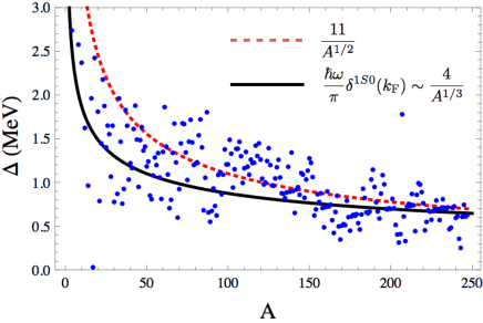
Figure 1: BCS pairing gap for the ${}^{1}S_{0}$-state (in ${\rm MeV}$) obtained from the on-shell phase-shift formula. We compare with double-differences from stable nuclei for $16<A<250$. We also show the conventional semiempirical mass formula yields $\Delta=11~{}A^{-1/2}$.

II Mass number dependence of pairing gap

In this section we review some of the nuclear mass fits favoring a $A^{-1/3}$ dependence of the pairing gap. This is not intended to be exhaustive but rather to show that a large variety of approaches and schemes merge into a single and unified pattern.

Vogel et al. questioned the Bohr-Mottelson formula Vogel:1984jyh providing instead $\Delta=7.1~{}A^{-1/3}~{}{\rm MeV}$ for the symmetric case $N=Z$. We will refer to this case hereafter and quote $\Delta$ in ${\rm MeV}$. Soon thereafter it was found a significant difference between protons and neutrons with $\Delta_{p}=7.55~{}A^{-1/3}$ and $\Delta_{n}=7.36~{}A^{-1/3}$ respectively Jensen:1984uok . A better description with a mean standard deviation of $0.18~{}{\rm MeV}$ is obtained from fourth order finite differences when comparing the $A^{-1/2}$ vs the $A^{-1/3}$ obtaining $\Delta=6.2~{}A^{-1/3}$ Madland:1988vix ; Moller:1992zz with satisfactory statistical properties for the residuals. An analysis of nuclear masses of $1654$ ground state nuclei with $N,Z\geq 8$ within a Thomas-Fermi model including several corrections with RMS deviation in the fit to masses of $0.655~{}{\rm MeV}$ needs $\Delta=6.03~{}A^{-1/3}$ Myers:1995wx . A direct analysis for $N\approx Z$ nuclei has lead to $\Delta=6.24~{}A^{-1/3}$ Vogel:1998km . The disentanglement between pairing and deformation in the odd-even staggering of nuclear masses has also revealed the inconsistency of the $A^{-1/2}$ dependence Satula:1998ha . A proton-neutron pairing study in a microscopic deformed BCS approach for Ge isotopes $A=64-76$ confirms better agreement with the $A^{-1/3}$ dependence than with the traditional $A^{-1/2}$ behavior Scaronimkovic:2003xv . The mass number dependence of nuclear pairing has also been investigated in Hilaire:2002yv using large scale Hartree-Fock-Bogoliubov calculations finding an average gap of $\Delta_{p}=4.52~{}A^{-1/3}$ and $\Delta_{n}=4.9\,A^{-1/3}$. Odd-even mass differences from self-consistent mean-field theory studies yield $\Delta_{p}=4.31~{}A^{-0.31}$ and $\Delta_{n}=4.55~{}A^{-0.31}$ Bertsch:2008yc . The implementation of a new pairing term in the Duflo-Zucker formulaMendozaTemis:2009ia yields $\Delta_{n}=5.0943~{}A^{-1/3}$. Following the pairing form of this reference, several determinations based on different schemes essentially confirm this value. In the improved Janecke mass formula it is found that $\Delta=4.9644~{}A^{-1/3}$ He:2014aaa , $\Delta=5.5108~{}A^{-1/3}$ Wang:2010dm or imposing mirror nuclei constraint in the mass formula $\Delta=5.4423~{}A^{-1/3}$ Wang:2010uk . Uncertainties have been evaluated, providing $\Delta=5.396(137)~{}A^{-1/3}$ Qi:2014cqa . An improved nuclear mass formula with a unified prescription for the shell and pairing corrections using explicitly BCS theory obtains $\Delta=7.5~{}A^{-1/3}$ with a remarkable gaussian distribution of residuals Zhang:2014txa . Direct fits to four point difference formulas are compatible with a variety of mass number dependencies, but when the $A^{-1/3}$ behavior is assumed one obtains $\Delta_{p}=6.26(4)~{}A^{-1/3}$ and $\Delta_{n}=6.22(4)~{}A^{-1/3}$ Ishkhanov:2014tra . The approach for the fluctuations based on a Fourier decomposition produces $\Delta=5.9~{}A^{-1/3}$ Bhagwat:2014jca and m.s.d. of $0.266~{}{\rm MeV}$ for $2353$ nuclei. The neural network approach to the fit including experimental uncertainties with the previous mass formula in the masses provides $\Delta=5.91(25)~{}A^{-1/3}$ Zhang:2017zvb . A three-point fit including a Wigner energy term yields $\Delta=5.319(236)~{}A^{-1/3}$ in Ref. Cheng:2015sca .

These studies describe a large body, typically about $2000$, of nuclear masses with mass formulas containing $10-20$ parameters, including a pairing term scaling as $A^{-1/3}$ which are determined by least squares minimization to the experimental nuclear masses database. While experimental accuracy cannot be obtained, they produce a mean standard deviations between $0.2-0.5~{}{\rm MeV}$ for the total mass. This makes in our view a strong case for this persistent $A^{-1/3}$ mass number dependence which demands a microscopic explanation. For $N=Z$ it can be summarized as in terms of the mean and standard deviation of all the studies cited above

$$\Delta\sim 6(1)~{}A^{-1/3}~{}{\rm MeV}\,.$$ (3)

The $15\%$ uncertainty reflects the disparity of the methods and most likely can be reduced by a judicious weighting, so that it can be interpreted as a systematic error, but it does show the robustness of all the approaches as a whole.

In this work we will provide such a microscopic explanation within the conventional BCS theory taking advantage of the freedom in the definition of the $NN$ interaction and also the fact that there is a natural discretization of momenta reflecting the finite size of the atomic nucleus. Obviously, we expect the continuum limit to correspond to a translationally invariant system.

III Effective $NN$ interactions and BCS equations in Nuclear Matter

In this section we review the basic elements of BCS theory in a translationally invariant system such as nuclear or neutron matter to fix our notation (see e.g. Refs. bohr1998nuclear ; ring2004nuclear ; Dean:2002zx for more details). The BCS state provides a paring gap given by

$$\Delta({\bf k})=-\frac{1}{2}\int\frac{d^{3}{\bf p}}{(2\pi)^{3}}\frac{V({\bf k},{\bf p})\Delta({\bf p})}{E({\bf p})}\;,$$ (4)

where $E({\bf p})^{2}=[({\bf p}^{2}-p_{F}^{2})/(2M)]^{2}+\Delta({\bf p})^{2}$ ($M$ is the nucleon mass) and the normalization conventions for the three dimensional LS equation are

$$T({\bf k},{\bf p})=V({\bf k},{\bf p})+\int\frac{d^{3}{\bf q}}{(2\pi)^{3}}\frac{V({\bf k},{\bf q})T({\bf q},{\bf p})}{{\bf p}^{2}/2\mu-q^{2}/2\mu}\;,$$ (5)

where $2\mu=M$, i.e. for a local potential

$$V({\bf k},{\bf p})=\int d^{3}{\bf x}V({\bf x})e^{-i({\bf k}-{\bf p}){\bf x}}\;.$$ (6)

After the partial-wave (PW) decomposition,

$$V^{S}({\bf p}^{\prime},{\bf p})=\frac{4\pi^{2}}{M}\sum_{JMLL^{\prime}}{\cal Y}_{LS}^{JM}(\hat{p}^{\prime})V_{LL^{\prime}}^{JS}(p^{\prime},p){{\cal Y}_{L^{\prime}S}^{JM}}^{\dagger}(\hat{p})\;,$$ (7)

and

$$\Delta^{S}({\bf p})=\sum_{JML}{\cal Y}_{LS}^{JM}(\hat{p})\Delta_{L}^{JS}(p)\;,$$ (8)

we have Dean:2002zx ,

$$\Delta_{L}^{J}(p)=-\frac{1}{\pi}\int_{0}^{\infty}p^{2}dp\sum_{L^{\prime}}\frac{V_{L,L^{\prime}}^{J}(k,p)\Delta_{L^{\prime}}^{J}(p)}{ME(p)}\;,$$ (9)

which is the generalized gap equation in all channels. Here $\Delta$ is in ${\rm fm}^{-1}$ and $V$ is in fm. These equations are solved iteratively until convergence is achieved. The pairing gap in a given channel is defined as $\Delta_{F}=\Delta(p)|_{p=p_{F}}$.

In this paper we will restrict our analysis to the simplest ${}^{1}S_{0}$ channel where the LS equation reads (we omit channel indices)

$$T(k^{\prime},k)=V(k^{\prime},k)+\frac{2}{\pi}\int_{0}^{\infty}dqV(k^{\prime},q)\frac{q^{2}}{k^{2}-q^{2}}T(q,k)\;,$$ (10)

The imaginary part of the T-matrix, ${\rm Im}T(k^{\prime},k)$, is fixed by unitarity. Passing to the reaction matrix defined by the real part $K(k^{\prime},k)={\rm Re}\,T(k^{\prime},k)$ we get

$$K(k^{\prime},k)=V(k^{\prime},k)+\frac{2}{\pi}\mathchoice{{\vbox{\hbox{$\textstyle-$}}\kern-4.86108pt}}{{\vbox{\hbox{$\scriptstyle-$}}\kern-3.25pt}}{{\vbox{\hbox{$\scriptscriptstyle-$}}\kern-2.29166pt}}{{\vbox{\hbox{$\scriptscriptstyle-$}}\kern-1.875pt}}\!\int_{0}^{\infty}dqV(k^{\prime},q)\frac{q^{2}}{k^{2}-q^{2}}K(q,k)\;,$$ (11)

whence the phase shift reads

$$\tan\delta(k)=-\frac{K(k,k)}{k}\;.$$ (12)

On the other hand, for the ${}^{1}S_{0}$ channel the BCS equation becomes

$$\Delta(k)=-\frac{1}{\pi}\int_{0}^{\infty}p^{2}dp\frac{V(k,p)\Delta(p)}{ME(p)}\;,$$ (13)

Realistic and effective $NN$ interactions, $V(k^{\prime}k)$, have been used to compute the pairing gap for nuclear and neutron matter in several schemes Dean:2002zx . Most often the BCS approach is based on having the scattering phase-shift as the basic input of the calculation. On the other hand, there is an arbitrariness in this procedure, as there are infinitely many interactions leading to the identical phase-shift. In this paper we analyze these ambiguities.

For instance, in the case of the pairing gap in the ${}^{1}S_{0}$ channel, most $V_{\rm low-k}$ calculations (not surprisingly) provide a BCS gap which has maximum at Fermi momentum $p_{F}\sim 0.8~{}{\rm fm}^{-1}$ and strength about $3~{}{\rm MeV}$ Sedrakian:2003cc ; Hebeler:2006kz . Chiral pion dynamics has been advocated in Ref. Kaiser:2004uj with similar results. We consider this as an educated guess for the total gap including polarization and short-distance correlations since ab initio calculations may provide completely different results Gezerlis:2009iw ; Gandolfi:2009tv ; Baldo:2010du . It is, however, disconcerting that the BCS gap is so different and so much scheme dependent.

There are claims in the literature that what determines the pairing gap are the phase-shifts Elgaroy:1997ti and finite nuclei calculations are carried out in Ref. Baroni:2009eh ; Idini:2011gm . We will see that this is not strictly true. In medium $T$-matrix has been used to provide an improvement on the standard BCS theory Bozek:2002ry yielding a 30% reduction in the ${}^{1}S_{0}$ pairing gap.

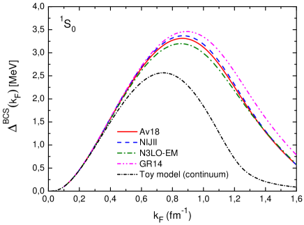
Figure 2: BCS pairing gap for the ${}^{1}S_{0}$-state in ${\rm MeV}$ of the toy model compared to realistic potentials AV18 Wiringa:1994wb , NijII Stoks:1994wp , N3LO-EM Entem:2003ft and GR14 Perez:2014yla , as a function of the Fermi momentum $k_{F}$ (in ${\rm fm}^{-1}$).

The previous equations neglect three- and many-body forces (see however Ref. Holt:2013vqa ; Furnstahl:2013oba ). While this may be a crude assumption, let us remind that disentanglement of three-body forces relies on the off-shellness of the interaction which can actually be traded for three-body forces. Thus, we will restrict ourselves to BCS many-body wave functions in a first approximation and will judge on the need of three-body forces at the end.

IV BCS pairing equations on a momentum grid

The BCS equations can be solved numerically on an $N$-dimensional momentum grid, $p_{1}<\dots p_{N}$  Szpigel:2010bj by implementing a high-momentum ultraviolet (UV) cutoff, $p_{\rm max}=\Lambda$, and an infrared (IR) momentum cutoff $p_{\rm min}=\Delta p$. The integration rule becomes

$$\int_{\Delta p}^{\Lambda}dpf(p)\to\sum_{n=1}^{N}w_{n}f(p_{n})\,.$$ (14)

The BCS equations on the grid follow from inserting the completeness relation in discretized momentum-space

$$1=\frac{2}{\pi}\sum_{n=1}^{N}w_{n}p_{n}^{2}|p_{n}\rangle\langle p_{n}|\,,$$ (15)

and defining the matrix-element as $V(p_{n},p_{m})\equiv\langle p_{n}|V|p_{m}\rangle$. For instance, the eigenvalue problem on the grid may be formulated as (bound states correspond to $P_{\alpha}=i\gamma$)

$$H\varphi_{\alpha}(p)=P_{\alpha}^{2}\varphi_{\alpha}(p)\,,$$ (16)

where the matrix representation of the hamiltonian reads

$$H(p_{n},p_{m})=p_{n}^{2}\delta_{n,m}+\frac{2}{\pi}w_{n}p_{n}^{2}V(p_{n},p_{m})\,.$$ (17)

Let us consider the BCS pairing gap equation on the grid

$$\Delta(p_{n})=-\frac{2}{\pi}\sum_{k=1}^{N}w_{k}p_{k}^{2}\frac{V(p_{n},p_{k})\Delta(p_{k})}{2ME(p_{n})}\;,$$ (18)

where $2ME(p_{n})=\sqrt{(p_{n}^{2}-p_{F}^{2})^{2}+4M^{2}\Delta(p_{n})^{2}}$. Of course, for consistency the Fermi momentum must also belong to the grid, $p_{F}=p_{m}$, so $2ME(p_{n})=\sqrt{(p_{n}^{2}-p_{m}^{2})^{2}+4M^{2}\Delta(p_{n})^{2}}$. We use an iterative method of solution (for several strategies see e.g. khodel1996solution ).

Solutions for the realistic potentials AV18 Wiringa:1994wb , NijII Stoks:1994wp , N3LO-EM Entem:2003ft and the more recent Granada potential (GR14) Perez:2014yla are displayed in Fig. 2 for a large number of grid points $N=200$ and a maximum momentum $p_{\rm max}=30~{}{\rm fm}^{-1}$.

Most analysis based on BCS usually end here. However, we want to stress that the only physical input information in these calculations is contained in the phase-shift but not in the potentials. As it is well known, this generates some off-shell ambiguity which cannot be directly related to measurable physical information Srivastava:1975eg . This off-shellness corresponds to the non-diagonal matrix elements of the potential $V(p^{\prime},p)$. In fact, one can make a unitary transformation $V\to UVU^{\dagger}$ such that phase-shifts remain invariant. In the next sections we will show that the BCS pairing gap can in principle depend strongly on this unitary transformation and hence on the off-shellness.

Besides, while the momentum grid is usually regarded as an auxiliary element for solving the BCS gap equation, we will show that it actually may be tailored to encode some relevant physical information, suggesting that in fact finite momentum grids may represent the finite size of the system. Moreover, we will show that using the inherent arbitrariness of the off-shellness in the potential one may get a large variety of results for the pairing gap. As a matter of fact, we will present a scheme which is free of any off-shell ambiguities, and for this scheme the continuum limit is shown to produce a vanishing BCS gap for an infinitely large system, as suggested by the abundant phenomenological large scale analysis quoted in Section II and suggesting $\Delta\sim a_{P}~{}A^{-1/3}$.

V Phase equivalent interactions and the on-shell limit

Quite generally, for a given hamiltonian we can always perform a unitary transformation $H\to UHU^{\dagger}$ keeping the phase-shift invariant. On the momentum grid $p_{n}$ with finite $N$ the definition of the phase-shift must be specified, since on the one hand one replaces the scattering boundary conditions with standing waves boundary conditions and on the other hand one wants to preserve the invariance under unitary transformations on the grid. As we have discussed in our previous work Arriola:2014fqa the energy-shift formula,

$$\delta^{\rm ES}(p_{n})=-\pi\frac{P_{n}^{2}-p_{n}^{2}}{2w_{n}p_{n}}\;,$$ (19)

with $P_{n}^{2}$ the $n-$th ordered eigenvalue, see Eq. (16), of the grid hamiltonian in Eq. (17) provides a suitable definition for the case where no bound states are present .

The unitary transformation $U$ can be quite general, and for our study we will generate them by means of the so-called Similarity Renormalization Group (SRG), proposed by Glazek and Wilson Glazek:1993rc ; Glazek:1994qc and independently by Wegner wegner1994flow who showed how high- and low-momentum degrees of freedom can decouple while keeping scattering equivalence.

The general SRG equation is given by Kehrein:2006ti ,

$$\frac{dH_{s}}{ds}=[[G_{s},H_{s}],H_{s}]\;,$$ (20)

and supplemented with a generator $G_{s}$ and an initial condition at $s=0$, $H_{0}$. This correspond to a one-parameter operator evolution dynamics and, as it is customary, we will often switch to the SRG cutoff variable $\lambda=s^{-1/4}$ which has momentum dimensions. The unitary character of the transformation follows from the trace invariance property ${\rm Tr}(H_{s})^{n}={\rm Tr}(H_{0})^{n}$ which holds due to the commutator, and hence $H_{s}=U_{s}H_{0}U_{s}^{\dagger}$. The generator $G_{s}$ can still be chosen according to certain requirements, and three popular choices are the kinetic energy $T$ Glazek:1994qc (Wilson-Glazek generator), the diagonal part of the Hamiltonian ${\rm Diag}(H)$ wegner1994flow (Wegner generator) or a block-diagonal (BD) generator $PH_{s}P+QH_{s}Q$ where $P+Q=1$ are orthogonal projectors $P^{2}=P$, $Q^{2}=Q$ , $QP=PQ=0$, for states below and above a given momentum scale Anderson:2008mu .

On the finite momentum grid the SRG equations become a set of non-linear coupled equations. For the Wegner generator, which will be taken here for definiteness, the equations take a quite simple form

$$\frac{dH_{s}(p_{n},p_{m})}{ds} = \frac{2}{\pi}\sum_{k}H_{s}(p_{n},p_{k})w_{k}p_{k}^{2}H_{s}(p_{k},p_{m})$$

$$\times \left[H_{s}(p_{n},p_{n})+H_{s}(p_{m},p_{m})-2H_{s}(p_{k},p_{k})\right]\;.$$

The fixed points of the SRG evolution with a given generator $G_{s}$ correspond to the stationary solutions of the SRG flow equations for the matrix-elements of the hamiltonian,

$$\frac{dH_{s}(p_{n},p_{m})}{ds}=\langle n|[[G_{s},H_{s}],H_{s}]|m\rangle=0\;,$$ (22)

which implies that in the infrared limit $s\to\infty$ ($\lambda\to 0$) the hamiltonian $H_{s}$ becomes diagonal, i.e.

$$\lim_{\lambda\to 0}H_{\lambda}(p_{n},p_{m})=P_{n}^{2}\delta_{nm}\;,$$ (23)

In this limit the potential $V_{\lambda}(p_{n},p_{m})$ also becomes diagonal, and the LS equation reaction matrix coincides with the potential. Thus, all off-shellness is eliminated in the SRG infrared limit $\lambda\to 0$. An important result derived in Ref. Arriola:2014fqa is

$$\delta_{n}^{G}=-\pi\lim_{\lambda\to 0}\frac{H_{n,n}^{G,\lambda}-p_{n}^{2}}{2w_{n}p_{n}}\;.$$ (24)

For this phase equivalent hamiltonian family, the BCS equation can be written as

$$\Delta_{\lambda}(p_{n})=-\sum_{k=1}^{N}\frac{[H_{\lambda}(p_{n},p_{k})-p_{n}^{2}\delta_{nk}]\Delta_{\lambda}(p_{k})}{2ME_{\lambda}(p_{n})}\;,$$ (25)

where $2ME_{\lambda}(p_{n})=\sqrt{(p_{n}^{2}-p_{F}^{2})^{2}+4M^{2}\Delta_{\lambda}(p_{n})^{2}}$. Clearly, the BCS pairing gap becomes a function of the SRG parameter $\lambda$, without ever changing the phase-shifts. Actually, in the infrared limit $\lambda\to 0$ the Hamiltonian becomes diagonal and hence we get

$$\Delta_{0}(p_{n})=-\frac{P_{n}^{2}-p_{n}^{2}}{2M}\frac{\Delta_{0}(p_{n})}{E_{0}(p_{n})}\;,$$ (26)

where the notation $\Delta_{0}(p_{n})\equiv\lim_{\lambda\to 0}\Delta_{\lambda}(p_{n})$ has been introduced. The solution is non trivial $\Delta_{0}(p_{n})\neq 0$ provided

$$1=-\frac{P_{n}^{2}-p_{n}^{2}}{2ME_{0}(p_{n})}\;,$$ (27)

and taking the grid point to be the Fermi momentum $p_{m}=p_{F}$ we get $E_{0}(p_{m})=\Delta_{0}(p_{m})$ and hence

$$\lim_{\lambda\to 0}\Delta_{\lambda}(p_{m})=\lim_{\lambda\to 0}-\frac{H_{\lambda}(p_{m},p_{m})-p_{m}^{2}}{2M}=w_{m}\frac{p_{m}\delta^{\rm ES}(p_{m})}{\pi M}\;.$$

Thus, the pairing gap is determined by the energy-shift at the Fermi surface in the ${}^{1}S_{0}$ channel for on-shell interactions. Not surprisingly, only the phase-shift appears in the final result. Note that since $\Delta_{0}(p_{m})\geq 0$ the equation makes sense only for $\delta(p_{m})\geq 0$. Note also, that the integration weights $w_{n}$ appear explicitly in the formula, and in the continuum limit $N\to\infty$ they vanish as $w_{n}={\cal O}(1/N)$ as expected . Therefore, if we denote by $\Delta p_{F}\equiv w_{F}$ the integration weight corresponding to the Fermi momentum, in the continuum limit the BCS pairing gap becomes

$$\Delta_{F}\sim\Delta p_{F}\frac{p_{F}\delta(p_{F})}{\pi M}$$ (29)

whenever $\Delta_{F}>0$ and zero otherwise. This is our main result. Note that while the shape is rather universal, the strength is related to $\Delta p_{F}$ which ultimately depends on the system size $R$ and geometry, and for large systems $\Delta p_{F}={\cal O}(1/R)$. While the simplicity of the result may look as being naive, in the next Section we will check by explicit numerical calculations, that Eq. (29) is indeed correct.

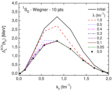
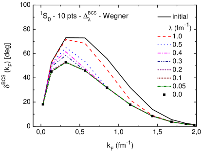
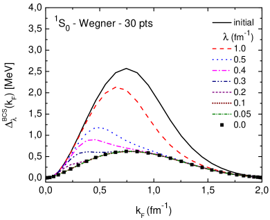
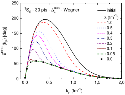
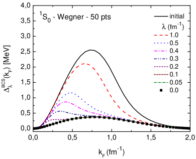
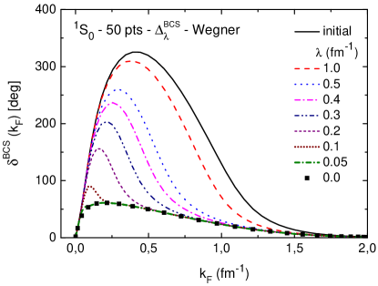
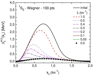
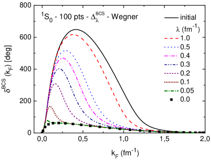
Figure 3: BCS pairing gap for the ${}^{1}S_{0}$-state in MeV (left panel) and the corresponding BCS phase-shift in degrees (right panel) as a function of the Fermi momentum $k_{F}$ (in ${\rm fm}^{-1}$). We show the SRG evolution for different values of the SRG cutoff $\lambda$ and for different number of grid points. In the left panel we also compare with the SRG invariant phase shift deduced as an energy shift.

VI Numerical Checks

It is interesting to analyze numerically the behavior of the pairing gap as a function of the SRG cut-off towards the on-shell limit. These are demanding calculations particularly with interactions having a strong short distance repulsive core which provide long momentum tails. Therefore and for computational reasons, in the present study of the ${}^{1}S_{0}$ neutron-neutron channel we will use the toy model gaussian separable potential discussed in our previous works Arriola:2013era ; Arriola:2014aia ; Arriola:2014fqa ; Arriola:2016fkr because the long momentum tails are suppressed from the start . For completeness we review the model in Appendix A. The performance of the toy model is rather good below for the phase-shifts below $p=1~{}{\rm fm}^{-1}$ Arriola:2013era . The resulting pairing gap can be obtained quite accurately as depicted in Fig. 2 and compared to some realistic potential calculations. As we see, and for our illustration purposes, it yields a sufficiently reasonable behavior compared to the realistic potentials AV18 Wiringa:1994wb , NijII Stoks:1994wp , N3LO-EM Entem:2003ft and GR14 Perez:2014yla . The good feature of the toy model is that when using the iterative method of solution khodel1996solution instead of $N=200$ and $p_{\rm max}=30~{}{\rm fm}^{-1}$ good convergence is achieved for $N=50$ and $p_{\rm max}=2~{}{\rm fm}^{-1}$.

In Fig. 3 we show the evolution of the pairing gaps $\Delta_{\lambda}(p_{n})$ obtained by solving the BCS equation on the grid as a function of the SRG cutoff $\lambda$ for the range $\lambda=1,\dots,0.05~{}{\rm fm}^{-1}$ and for several choices on the number of points $N=10,\dots,100$. Alternatively, we illustrate the scaling behavior of the BCS pairing gap by defining the “BCS phase-shift” as

$$\delta_{\lambda}^{\rm BCS}(p_{n})=\frac{\Delta_{\lambda}^{\rm BCS}(p_{n})\pi M}{w_{n}p_{n}}\;,$$ (30)

which, as expected, converges to the phase-shift obtained from the energy-shift formula, in the limit $\lambda\to 0$.

We note that along the SRG-trajectory the phase-shift remains constant if we take the energy-shift definition Arriola:2014aia as in Eq. (19), i.e.

$$\delta_{\lambda}^{\rm ES}(p_{n})=\delta_{\infty}^{\rm ES}(p_{n})=\delta_{0}^{\rm ES}(p_{n})\;.$$ (31)

Furthermore, we remind that as pointed out and illustrated in Ref. Arriola:2014aia the LS phase-shift, see Eq. (12), does not fulfill the phase-invariance on the finite grid, but only in the continuum limit, i.e. for $N\to\infty$. For reasons that will become clear below we are interested in having a definition, such as Eq. (30), of the phase-shift which is invariant along the SRG trajectory for any number of grid points N. It is important to emphasize that taking the on-shell situation corresponds to the infrared limit $\lambda\to 0$ Arriola:2013gya as the interaction becomes diagonal.

In Fig. 4 we show the limiting case $\lambda\to 0$ where now the pairing gap $\Delta^{\rm ES}(p_{n})$ on the grid is obtained from the SRG-invariant phase-shift computed from the energy-shift $\delta^{\rm ES}(p_{n})$.

The SRG evolution of the BCS pairing gap has been investigated in Ref. Maurizio:2014qsa for realistic potentials and for the range of values $\lambda=1-2~{}{\rm fm}^{-1}$ and for a relatively large momentum grid. The spread of BCS gap values has been interpreted as a measure of the uncertainty in the calculation, which we visualize in our results. However, we see no compelling reason to stop at their smallest SRG cutoffs besides numerical complications. As we see, when we take the limit $\lambda\to 0$, the gap is compatible with zero in the strict continuum limit.

The on-shell limit has been invoked previously for $A=3,4$ nuclei to provide an understanding of the Tjon line Arriola:2013gya ; Arriola:2016fkr as well as for unitary neutron matter Arriola:2014tva to determine the Bertsch parameter. On a finite grid it is important to check the onset of the on-shell limit. In many respects this has the properties of a phase transition where the order parameter is related to the Frobenius norm (see e.g. Arriola:2016fkr for a definition) as we have suggested recently Timoteo:2016vlp . In other words, for a finite $\Delta p$ one arrives at an on-shell behavior for $\lambda\gg\Delta p$. The insensitivity of binding of $A=3,4$ nuclei to the number of grid points has been explicitly shown in Refs. Arriola:2013gya ; Arriola:2016fkr . In summary, the onset of the on-shell regime of a discretized momentum system does not require the strict limit $\lambda\to 0$.

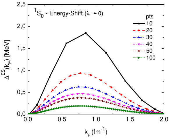
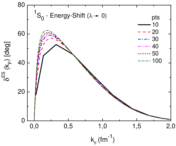
Figure 4: BCS pairing gap for the ${}^{1}S_{0}$-state in ${\rm MeV}$ (upper panel) and the corresponding BCS phase-shift in degrees (lower panel) as a function of the Fermi momentum $k_{F}$ (in ${\rm fm}^{-1}$) in the limit $\lambda\to 0$. In the upper panel we also compare with the SRG invariant phase shift deduced as an energy-shift.

VII The momentum grid in finite size system

Of course, the particular choice of the grid becomes irrelevant for our considerations, if we take it as a mere auxiliary scheme to solve the equations numerically. It is interesting, however, to consider grids corresponding to relevant physical situations, such as a finite size system as it is the case for finite nuclei. For instance in a spherical box of radius $R$ the momentum is quantized, $p_{n}\sim n\pi/R$, and in this case the spacing in momenta is uniform $\Delta p_{n}\sim\pi/R$.

Another way of implementing the finite size of the system is by using the harmonic oscillator basis with oscillator constant $b=\sqrt{\hbar/M\omega}$. Instead of doing this explicitly we will stay in the momentum basis but tune our discretized momenta to match harmonic oscillator wave functions. The equivalence between a momentum grid and a harmonic oscillator can be obtained from the differential equation at short distances since

$$-u_{nl}^{\prime\prime}+\left[\frac{l(l+1)}{r^{2}}+\frac{r^{2}}{b^{4}}\right]u_{nl}=p_{nl}^{2}u_{nl}\;,$$ (32)

so that for $r\ll b$ we have the free wave equation suggesting

$$u_{nl}^{\rm HO}(r)\sim j_{l}(p_{nl}r)\;.$$ (33)

The proportionality constant basis was fixed in kallio1965relation where

$$p_{nl}^{2}/2=(2n+l+3/2)/b^{2}$$ (34)

and thus $\Delta p_{F}\sim 1/b$. For a large volume fermionic system such as neutron or nuclear matter we can estimate, as usual, the value of $\hbar\omega$ by matching the total particle number, energy and radius of closed harmonic oscillator shells to the corresponding homogeneous Fermi gas in a finite volume. This provides a way of estimating the weight $w_{F}$ which corresponds to the momentum spacing at the Fermi momentum.

For instance, for neutron number $N$, the energy $E$ and the m.s.r. $\langle r^{2}\rangle$ of radius $R$, one gets

$$N = 2\sum_{nl}g_{nl}\to 2\int\frac{d^{3}kd^{3}x}{(2\pi)^{3}}\theta(k_{F}-k)\theta(R-r)\;,$$

$$E = 2\sum_{nl}g_{nl}e_{nl}\to 2\int\frac{d^{3}kd^{3}x}{(2\pi)^{3}}\epsilon_{k}\theta(k_{F}-k)\theta(R-r)$$

$$N\langle r^{2}\rangle = 2\sum_{nl}g_{nl}\langle r^{2}\rangle_{nl}\to 2\int\frac{d^{3}kd^{3}x}{(2\pi)^{3}}r^{2}\theta(k_{F}-k)\theta(R-r)\;.$$

Using the accidental degeneracy of the harmonic oscillator $2n+l=k$, so that $\sum_{nl}g_{nl}=\sum_{k=0}^{K}(k+1)(k+2)/2$, we have

$$\epsilon_{nl}=\hbar\omega(2n+l+3/2)\equiv\epsilon_{k}=\hbar\omega(k+3/2)\;$$ (36)

and

$$\langle r^{2}\rangle_{nl}=(b^{2}/\hbar\omega)\epsilon_{nl}\;.$$ (37)

In the limit of large $N$ we get $\hbar\omega\sim 1.78~{}N^{\frac{1}{3}}/(MR^{2})$ and $p_{F}\sim 12.05~{}N^{\frac{1}{3}}/R$ so that $\hbar\omega\sim 0.147~{}k_{F}/(MR)$ and hence the estimate of the pairing gap in a large but finite system is

$$\Delta(N,R)\sim\frac{1.78~{}N^{\frac{1}{3}}}{\pi MR^{2}}\delta\left(\frac{12.05~{}N^{\frac{1}{3}}}{R}\right)\;,$$ (38)

or equivalently

$$\Delta_{nn}(k_{F},R)\sim\frac{0.147~{}k_{F}}{\pi MR}\delta^{{}^{1}S_{0}}_{nn}\left(k_{F}\right)\;,$$ (39)

where $w_{F}=0.147/R$. Thus the pairing gap decreases with the size of the system. Repeating the same exercise for nuclear matter ring2004nuclear one obtains $\hbar\omega\sim 41~{}A^{-1/3}~{}{\rm MeV}$, $b=1.0~{}A^{\frac{1}{6}}{\rm fm}$ and $n_{\rm max}=1.58~{}A^{\frac{1}{3}}$, so that $\Delta p_{n_{\rm max}}^{2}=1/b^{2}$ and hence since $p_{n_{\rm max}}^{2}=2M\hbar\omega(n_{\rm max}+3/2)$ we have $\Delta p_{n_{\rm max}}=91~{}A^{-1/3}~{}{\rm MeV}$. So we have

$$\Delta_{n_{\rm max}} \sim \frac{\Delta p_{n_{\rm max}}^{2}}{2M}\frac{\delta(p_{n_{\rm nmax})}}{\pi}$$ (40)

$$= \frac{\hbar\omega}{\pi}\delta(p_{n_{\rm nmax}})=13~{}A^{-1/3}\delta(p_{n_{\rm nmax}})\;.$$

Actually, the corresponding semi-empirical mass formula pairing term yields a vanishingly small contribution for large $A$ while the size scales as $R=1.2~{}A^{\frac{1}{3}}~{}{\rm fm}$. Reinstating continuum notation the final formula reads

$$\Delta(p_{F})=\frac{\hbar\omega}{\pi}\delta(p_{F})\quad,\qquad\hbar\omega\sim 41\,A^{-1/3}~{}{\rm MeV}\,,$$ (41)

where the desired $A^{-1/3}$ can be read off. This is the main consequence of our main result.

For the typical values of the Fermi momentum around $k_{F}\sim 1~{}{\rm fm}^{-1}$ the phase-shift presents so linear dependent around $\delta(p)\sim 30^{0}$, so that Eq. (41) can numerically be approximated by $\Delta\sim 4\,A^{-1/3}~{}{\rm MeV}$. This result is compared to double-differences obtained from stable-nuclei data in Fig. 1. As we see, and given the fluctuations in the data, the performance looks of comparable quality as the textbook pairing term $11A^{-1/2}~{}{\rm MeV}$. Note, however, that after many other effects are explicitly taken into account this liquid drop model smooth behavior is not confirmed, as discussed in Section II. Ours is instead based directly on the available on-shell $NN$ scattering information relevant for the BCS pairing gap which not only reproduces the mass number behavior of the estimated pairing gap from large scale analysis $\Delta_{\rm exp}\sim 6(1)\,A^{-1/3}~{}{\rm MeV}$ but also accounts by $75\%$ of the coefficient.

These results are rather promising as they use the concept of on-shell interactions for a finite size system which we regard as the key aspect of the derivation. However, if we take the discrepancy seriously we see that there is still room for other effects. In what follows we consider the possibility that this might be due to three-body effects with the proviso that the very definition of the three-body force depends on the definition of the two body force and more specifically on its off-shell behaviour. For definiteness we will analyze this question within the SRG framework.

Of course, while evolving along the SRG trajectory we are on the one hand keeping the physical phase-shift constant but on the other hand we are also changing the off-shellness of the interaction striving to its diagonal on-shell form. The pairing gap is a physical quantity and we should not expect to depend on unphysical features. From that point of view, the change in the BCS pairing gap might be viewed as a genuine uncertainty limiting the predictive power. However, one may argue that there are three- and many-body forces guaranteeing the independence of the pairing gap on the calculational scheme. Unfortunately, within an SRG framework it is unclear at what SRG scale should the three-body forces be switched on. The prototype instances for the need of three- and four-body forces are the triton and helium binding energies. However, it is well known that assuming some high quality NN potentials as initial condition for the SRG evolution the need of NNN forces can be minimized by choosing appropriate $\lambda$-scales Deltuva:2008mv ; Jurgenson:2009qs ; Jurgenson:2010wy . Actually, in Ref. Deltuva:2008mv it is found that using the CD-Bonn and AV18 (but not N3LO) potentials that the triton binding energy can be obtained by taking $\lambda\sim 1.5{\rm fm}^{-1}$. In Refs. Jurgenson:2009qs ; Jurgenson:2010wy this is confirmed and in addition the helium binding is obtained also for about the same $\lambda\sim 1.5{\rm fm}^{-1}$. Actually, the universal linear correlation between the binding energies of helium and triton, known as Tjon line (see e.g. Ref. Hammer:2012id for a review and references therein), does not depend explicitly on a particular choice of three-body force; they only relate the equivalent trade-off of the different off-shellness Arriola:2013gya . This shows that for some moderate $\lambda$-scales three-body forces are not dominant.

As we have already mentioned the onset of the on-shell NN dynamics enjoys the features of a phase transition and for a given system the transition point depends on the momentum resolution and hence on the number of grid points Timoteo:2016vlp . In that work it was shown that using the N3LO potential, where $p_{\rm max}=4\,{\rm fm}^{-1}$ proves sufficient for convergence, the off-shell to on-shell transition takes place at $\lambda=0.9,1.1,1.5\,{\rm fm}^{-1}$ for $N=30,20,10$ respectively. This corresponds to $\Delta p\sim p_{\rm max}/N=0.13,0.2,0.4\,{\rm fm}^{-1}$ and taking $\Delta p=\pi/R$ to $R\sim 24,16,8\,{\rm fm}$ respectively. Therefore, for a system of size $R\sim 8\,{\rm fm}$ the N3LO becomes on-shell at about $\lambda\sim 1.5\,{\rm fm}^{-1}$. While these are rough estimates they show that the scenario in a finite system where NN forces are close to be on-shell takes place at about the same scales where three-body forces are not dominating.

Therefore we find that the pairing gap is largely shape independent and only the strength decreases with the system size. Moreover, we also see that this feature holds already for moderate SRG cutoffs, determined by the infrared momentum scale fixed by the finite system size, $\lambda\sim\Delta p\pi/R$, below which the on-shell regime sets in. From that point of view we expect finite but not large corrections to our results stemming from three-body forces.

In the BCS approximation it has been found that the effect of 3N body forces can effectively be included in the gap equation as a replacement of the NN interaction in the ${}^{1}S_{0}$ channel as Hebeler:2009iv

$$V_{NN}(p,k)\to V_{NN}(p,k)+\frac{1}{2}\bar{V}_{3N}(p,k)$$ (42)

where the average is understood in the 2-1 relative coordinate below the Fermi sea. A detailed analysis of this equation along the present lines is beyond the scope of our work, and it remains a challenge to obtain that, quite generally, for a large $A$ nucleus we may expect

$$\Delta=(a_{2N}+a_{3N}+\dots)A^{-1/3}+{\cal O}(A^{-2/3})$$ (43)

VIII Conclusions

In the present work we have explored the freedom on reducing the off-shellness of the $NN$ interaction as a way to analyze the BCS pairing gap. Quite remarkably, we find that there is an on-shell regime which depends on the size of the nucleus, where the BCS pairing gap corresponds to the energy shift at the Fermi surface due to the NN interaction, and can directly determined by the $NN$ phase-shifts in the ${}^{1}S_{0}$ channel. Our formula provides a satisfactory mass number dependence $\Delta=4~{}A^{-1/3}~{}{\rm MeV}$ which accounts for the bulk of the $\Delta=6(1)A^{-1/3}$ found by many nuclear mass analyses comprising over $2000$ masses and with a mean standard deviation of $0.2-0.5~{}{\rm MeV}$. The differences might most likely be attributed to three-body forces. This on-shell simplification on the finite size system neglects $3N$-forces and it remains a challenge to verify this mass number dependence when they are included in the calculation. The phenomenological success suggests analyzing more complicated situations and a thorough analysis of different channels in higher partial waves. Work along these lines is in progress.

Appendix A Toy model

In the present study of the ${}^{1}S_{0}$ neutron-neutron channel we use the toy model gaussian separable potential of the form

$$V(k^{\prime},k)=Cg(k^{\prime})g(k)$$ (44)

with $g(k)=e^{-k^{2}/L^{2}}$ discussed in our previous works Arriola:2013era ; Arriola:2014aia ; Arriola:2014fqa ; Arriola:2016fkr because it allows a handy SRG treatment in the infrared (see below). For this potential the LS equation, Eq. (10) can be solved by assuming $T(k^{\prime},k)=tg(k^{\prime})g(k)$ and leading to an explicit expression for the phase-shift using Eq. (12), namely

$$p\cot\delta_{0}(p) = -\frac{1}{V_{0}(p,p)}\left[1-\frac{2}{\pi}\mathchoice{{\vbox{\hbox{$\textstyle-$}}\kern-4.86108pt}}{{\vbox{\hbox{$\scriptstyle-$}}\kern-3.25pt}}{{\vbox{\hbox{$\scriptscriptstyle-$}}\kern-2.29166pt}}{{\vbox{\hbox{$\scriptscriptstyle-$}}\kern-1.875pt}}\!\int_{0}^{\infty}dq\frac{q^{2}}{p^{2}-q^{2}}V_{0}(q,q)\right]$$ (45)

$$= -\frac{1}{\alpha_{0}}+\frac{1}{2}r_{0}p^{2}+\dots$$

where in the last line a low-momentum Effective Range Expansion (ERE) has been carried out. Parameters $C$ and $L$ have been determined from the corresponding scattering length $\alpha_{0}$ and effective range $r_{0}$ in the ${}^{1}S_{0}$ channel and the resulting phase-shift is rather reasonable in the region of CM momentum below $p\sim 1~{}{\rm fm}^{-1}$ Arriola:2013era ; Arriola:2014aia ; Arriola:2014fqa ; Arriola:2016fkr . For this potential the BCS equation is readily solved by taking the ansatz

$$\Delta(k)=\Delta_{0}g(k)$$ (46)

where $\Delta_{0}$ satisfies the implicit equation

$$1=-\frac{1}{\pi}\int_{0}^{\infty}p^{2}dp\frac{C[g(p)]^{2}}{ME(p)}$$ (47)

and $4M^{2}E(p)^{2}=(p^{2}-p_{F}^{2})^{2}+4M^{2}\Delta_{0}^{2}g(p)^{2}$. The resulting pairing gap $\Delta_{F}\equiv\Delta_{0}g(p_{F})$ is depicted in Fig. 2 and compared to some realistic potential calculations and, as we see, yields a reasonable description.

References

- (1) A. Bohr, B. Mottelson and D. Pines, Phys.Rev. 110 (1958) 936.
- (2) A. Bohr and B.R. MottelsonNuclear structure Vol. 1 (World Scientific, 1998).
- (3) P. Ring and P. Schuck, The nuclear many-body problem (Springer Science & Business Media, 2004).
- (4) D. Dean and M. Hjorth-Jensen, Rev.Mod.Phys. 75 (2003) 607, nucl-th/0210033.
- (5) W. Satula, Phys.Scripta T125 (2006) 82, nucl-th/0508066.
- (6) J. Toivanen et al., Phys.Rev. C78 (2008) 034306, 0806.1914.
- (7) N. Fukuda and R.G. Newton, Phys. Rev. 103 (1956) 1558.
- (8) B.S. DeWitt, Phys. Rev. 103 (1956) 1565.
- (9) M.K. Srivastava and D.W.L. Sprung, (1975).
- (10) P. Vogel, B. Jonson and P.G. Hansen, Phys. Lett. 139B (1984) 227.
- (11) A.S. Jensen, P.G. Hansen and B. Jonson, Nucl. Phys. A431 (1984) 393.
- (12) D.G. Madland and J.R. Nix, Nucl. Phys. A476 (1988) 1.
- (13) P. Moller and J.R. Nix, Nucl. Phys. A536 (1992) 20.
- (14) W.D. Myers and W.J. Swiatecki, Nucl. Phys. A601 (1996) 141.
- (15) P. Vogel, Nucl. Phys. A662 (2000) 148, nucl-th/9805015.
- (16) W. Satula, J. Dobaczewski and W. Nazarewicz, Phys. Rev. Lett. 81 (1998) 3599, nucl-th/9804060.
- (17) F. Scaronimkovic et al., Phys. Rev. C68 (2003) 054319.
- (18) S. Hilaire et al., Phys. Lett. B531 (2002) 61, nucl-th/0206067.
- (19) G.F. Bertsch et al., Phys. Rev. C79 (2009) 034306, 0812.0747.
- (20) J. Mendoza-Temis, J.G. Hirsch and A.P. Zuker, Nucl. Phys. A843 (2010) 14, 0912.0882.
- (21) Z. He et al., Phys. Rev. C90 (2014) 054320.
- (22) N. Wang, M. Liu and X. Wu, Phys. Rev. C81 (2010) 044322, 1001.1493.
- (23) N. Wang et al., Phys. Rev. C82 (2010) 044304, 1008.2115.
- (24) C. Qi, J. Phys. G42 (2015) 045104, 1407.8221.
- (25) H. Zhang et al., Nucl. Phys. A929 (2014) 38.
- (26) B.S. Ishkhanov, M.E. Stepanov and T.Yu. Tretyakova, Moscow Univ. Phys. Bull. 69 (2014) 1, [Vestn. Mosk. Univ.,no.1,3(2014)].
- (27) A. Bhagwat, Phys. Rev. C90 (2014) 064306.
- (28) H.F. Zhang et al., J. Phys. G44 (2017) 045110.
- (29) Y.Y. Cheng et al., Phys. Rev. C91 (2015) 024313.
- (30) A. Sedrakian et al., Phys.Lett. B576 (2003) 68, nucl-th/0308068.
- (31) K. Hebeler, A. Schwenk and B. Friman, Phys.Lett. B648 (2007) 176, nucl-th/0611024.
- (32) N. Kaiser, T. Niksic and D. Vretenar, Eur.Phys.J. A25 (2005) 257, nucl-th/0411038.
- (33) A. Gezerlis and J. Carlson, Phys.Rev. C81 (2010) 025803, 0911.3907.
- (34) S. Gandolfi et al., Phys.Rev. C80 (2009) 045802, 0907.1588.
- (35) M. Baldo et al., J.Phys.G G37 (2010) 064016, 1001.0743.
- (36) O. Elgaroy and M. Hjorth-Jensen, Phys.Rev. C57 (1998) 1174, nucl-th/9708026.
- (37) S. Baroni, A.O. Macchiavelli and A. Schwenk, Phys.Rev. C81 (2010) 064308, 0912.0697.
- (38) A. Idini, F. Barranco and E. Vigezzi, Phys.Rev. C85 (2012) 014331, 1107.0251.
- (39) P. Bozek and P. Czerski, Phys.Rev. C66 (2002) 027301, nucl-th/0204012.
- (40) R.B. Wiringa, V. Stoks and R. Schiavilla, Phys.Rev. C51 (1995) 38, nucl-th/9408016.
- (41) V. Stoks et al., Phys.Rev. C49 (1994) 2950, nucl-th/9406039.
- (42) D. Entem and R. Machleidt, Phys.Rev. C68 (2003) 041001, nucl-th/0304018.
- (43) R. Navarro Perez, J. Amaro and E. Ruiz Arriola, Phys.Rev. C89 (2014) 064006, 1404.0314.
- (44) J. Holt, J. Menendez and A. Schwenk, J.Phys. G40 (2013) 075105, 1304.0434.
- (45) R. Furnstahl and K. Hebeler, Rept.Prog.Phys. 76 (2013) 126301, 1305.3800.
- (46) S. Szpigel, V.S. Timóteo and F.d.O. Duraes, Annals Phys. 326 (2011) 364, 1003.4663.
- (47) V. Khodel, V. Khodel and J. Clark, Nuclear Physics A 598 (1996) 390.
- (48) E.R. Arriola, S. Szpigel and V.S. Timóteo, (2014), 1407.8449.
- (49) S.D. Glazek and K.G. Wilson, Phys.Rev. D48 (1993) 5863.
- (50) S.D. Glazek and K.G. Wilson, Phys. Rev. D49 (1994) 4214.
- (51) F. Wegner, Annalen der physik 506 (1994) 77.
- (52) S. Kehrein, The flow equation approach to many-particle systems (Springer, 2006).
- (53) E. Anderson et al., Phys.Rev. C77 (2008) 037001, 0801.1098.
- (54) E. Ruiz Arriola, S. Szpigel and V. Timóteo, Phys.Lett. B728 (2014) 596, 1307.1231.
- (55) E. Ruiz Arriola, S. Szpigel and V. Timóteo, (2014), 1404.4940.
- (56) E. Ruiz Arriola, S. Szpigel and V.S. Timóteo, Annals Phys. 371 (2016) 398, 1601.02360.
- (57) F. Tabakin, Phys.Rev. 177 (1969) 1443.
- (58) E. Ruiz Arriola, S. Szpigel and V. Timóteo, Few Body Syst. 55 (2014) 971, 1310.8246.
- (59) S. Maurizio, J. Holt and P. Finelli, (2014), 1408.6281.
- (60) E. Ruiz Arriola, S. Szpigel and V.S. Timóteo, J. Phys. Conf. Ser. 630 (2015) 012036, 1412.2077.
- (61) V.S. Timóteo, E. Ruiz Arriola and S. Szpigel, Few Body Syst. 58 (2017) 62, 1611.06799.
- (62) A. Kallio, Physics Letters 18 (1965) 51.
- (63) A. Deltuva, A.C. Fonseca and S.K. Bogner, Phys. Rev. C77 (2008) 024002, 0802.1472.
- (64) E.D. Jurgenson, P. Navratil and R.J. Furnstahl, Phys. Rev. Lett. 103 (2009) 082501, 0905.1873.
- (65) E.D. Jurgenson, P. Navratil and R.J. Furnstahl, Phys. Rev. C83 (2011) 034301, 1011.4085.
- (66) H.W. Hammer, A. Nogga and A. Schwenk, Rev.Mod.Phys. 85 (2013) 197, 1210.4273.
- (67) K. Hebeler and A. Schwenk, Phys. Rev. C82 (2010) 014314, 0911.0483.