Quantifying uncertainty in state and parameter estimation

Abstract

Observability of state variables and parameters of a dynamical system from an observed time series is analyzed and quantified by means of the Jacobian matrix of the delay coordinates map. For each state variable and each parameter to be estimated a measure of uncertainty is introduced depending on the current state and parameter values, which allows us to identify regions in state and parameter space where the specific unknown quantity can (not) be estimated from a given time series. The method is demonstrated using the Ikeda map and the Hindmarsh-Rose model.

180(18,262) Copyright 2014 by the American Physical Society. The following article appeared in U. Parlitz, et al., Phys. Rev. E 89, 050902(R) (2014) and may be found at http://dx.doi.org/10.1103/PhysRevE.89.050902. In physics and other fields of science including quantitative biology, life sciences, and climatology, mathematical models play a crucial role for understanding and predicting dynamical processes. In the following we assume that such a model exists and is known. But even in the ideal case of a model obtained from fundamental physical laws this model typically contains some parameters whose values have to be determined depending on the physical context. Furthermore, not all state variables of the model may be easily experimentally accessible. To estimate the unknown parameters and state variables you may either devise specific experiments focusing on the quantity of interest or you can try to extract the required information from a measured time series of the process to be modeled. Technically, several estimation methods exist, including observer or synchronization schemes PJK96 ; NM97 ; HLN01 ; GB08 ; ACJ08 ; SO09 , particle filters L10 , a path integral formalism A09 ; QA10 , or optimization based algorithms CGA08 ; B10 ; SBP11 . However, these methods may fail and at this point the question arises whether the failure is due to the specific algorithm used or due to a lack of information in the available time series. In this article we address the second option and present a general approach for answering the question whether a given time series enables the estimation of parameters or variables of interest in a given model. The mathematical tool that is used to answer this question is delay reconstruction Aeyels ; Takens ; SYC91 ; KS97 ; book_HDIA and the basic criterion for local observability is the rank of the Jacobian matrix of the delay coordinates map. This approach was motivated by work of Letellier, Aguirre, and Maquet LAM05 ; LA09 ; FBL12 who studied the question which state variables can be estimated or observed from a given time series using derivative coordinates. Observability of (continuous) dynamical system is also a major issue in control theory HK77 ; Sontag ; N82 and nonlinear time series analysis VTK04 . Here we consider discrete time and delay coordinates, and we introduce a quantitative measure of uncertainty which in general varies on the attractor and thus indicates where in state space estimation is more efficient and less error prone. Furthermore, we focus not only on state variables but also on observability of model parameters.

Let’s assume, first, that our model of interest is a $M$-dimensional discrete dynamical system

$${\mathbf{x}}(n+1)={\mathbf{g}}[{\mathbf{x}}(n),\mathbf{p}]$$ (1)

given by an iterated function $\mathbf{g}$ depending on the state vector $\mathbf{x}(n)=(x_{1}(n),\ldots,x_{M}(n))\in\mathbb{R}^{M}$ at time $n$ and $K$ parameters $\mathbf{p}=(p_{1},\ldots,p_{K})\in\mathbb{R}^{K}$. This system generates the times series $\{s(n)\}$ with $s(n)=h({\bf x}(n))$ (for $n=1,\ldots,N$), where $h$ denotes a measurement or observation function. The time series $\{s(n)\}$ can be used to construct a $D$ dimensional delay reconstruction Aeyels ; Takens ; SYC91 ; KS97 ; book_HDIA ,

$${\mathbf{y}} = \left(s(n),s(n+1),....,s(n+D-1)\right)$$

$$= G({\mathbf{x}},\mathbf{p})\in\mathbb{R}^{D}$$

providing the delay coordinates map $G:\mathbb{R}^{M+K}\to\mathbb{R}^{D}$.

To uniquely recover the full state $\mathbf{x}$ and the parameters $\mathbf{p}$ from the observations represented by the reconstructed state $\mathbf{y}$ the map $G$ has to be locally invertible. More precisely, let $M+K\leq D$ and let $(\mathbf{x},\mathbf{p})\in{\cal{U}}$ where ${\cal{U}}\subset\mathbb{R}^{M+K}$ is a smooth manifold. Then $G$ is locally invertible on the image $G({\cal{U}})\subset\mathbb{R}^{D}$ if the $D\times(M+K)$ Jacobian matrix $DG(\mathbf{x},\mathbf{p})$ has full rank $M+K$ (i.e., $G$ is an immersion SYC91 ).

The map from delay reconstruction space $\mathbb{R}^{D}$ to the state and parameter space $\mathbb{R}^{M+K}$ is locally given by the (pseudo) inverse of the Jacobian matrix $DG$ of the delay coordinates map $G$, which can be computed using a singular value decomposition

$$DG=USV^{\text{tr}}$$ (3)

where $S=\rm{diag}(\sigma_{1},\ldots,\sigma_{M+K})$ is a $(M+K)\times(M+K)$ diagonal matrix containing the singular values $\sigma_{1}\geq\sigma_{2}\geq\ldots\geq\sigma_{M+K}\geq 0$ and $U=(\mathbf{u}^{(1)},\ldots,\mathbf{u}^{(M+K)})$ and $V=(\mathbf{v}^{(1)},\ldots,\mathbf{v}^{(M+K)})$ are orthogonal matrices, represented by the column vectors $\mathbf{u}^{(i)}\in\mathbb{R}^{D}$ and $\mathbf{v}^{(i)}\in\mathbb{R}^{M+K}$, respectively. $V^{\text{tr}}$ is the transposed of $V$ coinciding with the inverse $V^{-1}=V^{\text{tr}}$. Analogously, $U^{\text{tr}}=U^{-1}$ and the (pseudo) inverse Jacobian matrix reads $DG^{-1}=VS^{-1}U^{\text{tr}}$ where $S^{-1}=\rm{diag}(1/\sigma_{1},\ldots,1/\sigma_{M+K})$. Multiplying by $U$ from the right we obtain $DG^{-1}U=VS^{-1}$ or

$$DG^{-1}\mathbf{u}^{(j)}=\frac{1}{\sigma_{j}}\mathbf{v}^{(j)}\ \ \ \ \ (j=1,\ldots,M+K).$$ (4)

In Fig. 1 the transformation of singular vectors Eq. (4) is illustrated for the case $M=2$ and $K=0$ (no unknown parameters). The diagram shows how small perturbations of $\mathbf{y}$ in delay reconstruction space result in deviations from $\mathbf{x}$ in the original state space. Most relevant for the local observability of the (original) state $\mathbf{x}$ is the length of the longest principal axis of the ellipsoid given by the inverse of the smallest singular value $\sigma_{2}$ (see Fig. 1). Small singular values correspond to directions in state space, where it is difficult (or even impossible) to locate the true state $\mathbf{x}$ given a finite precision of the reconstructed state $\mathbf{y}$. The ratio $\sigma_{\text{min}}/\sigma_{\text{max}}$ of the smallest and the largest singular value is a measure of observability at the reference state $\mathbf{x}$. By averaging on the attractor we define (analogously to a similar definition for derivative coordinates LAM05 ; LA09 ) the observability index

$$\bar{\gamma}=\frac{1}{N}\sum_{n=1}^{N}\frac{\sigma_{\text{min}}^{2}(\mathbf{x})}{\sigma_{\text{max}}^{2}(\mathbf{x})}.$$ (5)

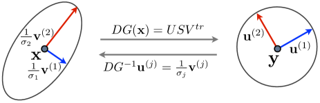
Figure 1: (Color online) The (pseudo) inverse Jacobian matrix $DG^{-1}(\mathbf{y})$ maps perturbations of $\mathbf{y}$ in delay reconstruction space to deviations from the state $\mathbf{x}$ whose magnitudes depend on the direction of the perturbation as described by Eq. (4).

If the perturbations of $\mathbf{y}$ are due to normally distributed measurement noise than they can be described by a symmetric Gaussian distribution centered at $\mathbf{y}$

$$Q(\mathbf{\tilde{y}})=\frac{\exp\left[-\frac{1}{2}({\mathbf{\tilde{y}}}-{\mathbf{y}})^{\text{tr}}\Sigma_{y}^{-1}({\mathbf{\tilde{y}}}-{\mathbf{y}})\right]}{\sqrt{(2\pi)^{D}\det(\Sigma_{y})}}$$ (6)

where $\mathbf{\tilde{y}}$ is the perturbed state, $\Sigma_{y}={\rm{diag}}(\rho^{2},\ldots,\rho^{2})=\rho^{2}I_{D}$ denotes the $D\times D$ covariance matrix ($I_{D}$ stands for the $D$-dimensional unit matrix), and the standard deviation $\rho$ quantifies the noise amplitude. For (infinitesimally) small perturbations $\mathbf{\Delta y}=\mathbf{\tilde{y}}-\mathbf{y}$ this distribution is mapped by the pseudo inverse of the linearized delay coordinates map to the (non-symmetrical) distribution

$$P(\mathbf{\tilde{x}})=\frac{\exp\left[-\frac{1}{2}(\mathbf{\tilde{x}}-\mathbf{x})^{\text{tr}}\Sigma_{x}^{-1}(\mathbf{\tilde{x}}-\mathbf{x})\right]}{\sqrt{(2\pi)^{M+K}\det(\Sigma_{x})}}$$ (7)

centered at $\mathbf{x}$ with the inverse covariance matrix

$$\begin{array}[]{rcl}\Sigma_{x}^{-1}&=&DG^{\text{tr}}\Sigma_{y}^{-1}DG\\ &=&\frac{1}{\rho^{2}}DG^{\text{tr}}DG=\frac{1}{\rho^{2}}VS^{2}V^{\text{tr}}.\end{array}$$ (8)

The marginal distribution $P_{j}$ of the $j$th state variable centered a $x_{j}$ is given by

$$P_{j}(\tilde{x}_{j})=\frac{1}{\rho_{j}\sqrt{2\pi}}\exp\left[-\frac{(\tilde{x}_{j}-x_{j})^{2}}{2\rho_{j}^{2}}\right]\,,$$ (9)

where the standard deviation $\rho_{j}$ is given by the square root of the diagonal elements of the covariance matrix $\rho_{j}=\sqrt{\Sigma_{x,jj}}$ that can be obtained by inverting $\Sigma_{x}^{-1}$ [given in Eq. (8)]. Since the noise level $\rho$ of the observations appears in Eq. (8) as a factor only we can, without loss of generality, choose $\rho=1$ and use

$$\nu_{j}=\sqrt{\left[DG^{\text{tr}}DG\right]^{-1}_{jj}}=\sqrt{\left[VS^{-2}V^{\text{tr}}\right]_{jj}}$$ (10)

as a measure of uncertainty when estimating $x_{j}$, which can be interpreted as a noise amplification factor. The same reasoning holds for the unknown parameters $\mathbf{p}$.

To illustrate this quantification of observability we first consider the Ikeda map I79 $z(n+1)=p_{1}+p_{2}z(n)\exp[ip_{3}-ip_{4}/(1+|z(n)|^{2})]$ with $z(n)=x_{1}(n)+ix_{2}(n)\in\mathbb{C}$ that can also be written as

$$\begin{array}[]{rcl}x_{1}(n+1)&=&p_{1}+p_{2}[x_{1}(n)\cos\theta_{n}-x_{2}(n)\sin\theta_{n}]\\ x_{2}(n+1)&=&p_{2}[x_{1}(n)\sin\theta_{n}+x_{2}(n)\cos\theta_{n}]\end{array}$$ (11)

where $\theta_{n}=p_{3}-p_{4}/[1+x_{1}^{2}(n)+x_{2}^{2}(n)]$. For the standard parameters $p_{1}=1$, $p_{2}=0.9$, $p_{3}=0.4$, and $p_{4}=6$ this map generates the chaotic attractor shown in Fig. 2.

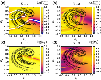
Figure 2: (Color online) Observability of the state variables $x_{1}$ and $x_{2}$ of the Ikeda map Eq. (11) from a $x_{1}$ time series (with known parameters, $K=0$, $M=2$). (a), (b) Color-coded ratio of singular values $\sigma_{\text{min}}/\sigma_{\text{max}}$ vs. $x_{1}$ and $x_{2}$ for reconstruction dimension $D=2$ (a) and $D=3$ (b). The white curves in (a) indicate the location of zeros of $\det(DG)$. (c), (d) Color-coded uncertainties $\nu_{1}$ (c) and $\nu_{2}$ (d) of $x_{1}$ and $x_{2}$ estimates, respectively. Note the logarithmic color axes. Black dots represent the Ikeda attractor.

First, we consider a case where all parameters are known and only the variables $x_{1}$ and $x_{2}$ have to be estimated from the observable $s(n)=x_{1}(n)$ (i.e., $M=2$ and $K=0$). Figures 2(a) and 2(b) show (color-coded) the ratio of the smallest singular value $\sigma_{\text{min}}=\sigma_{M}$ and the largest singular value $\sigma_{\text{max}}=\sigma_{1}$ of the Jacobian matrix $DG(\mathbf{x})$ of the delay coordinates map vs. $x_{1}$ and $x_{2}$. Reconstruction dimensions are $D=2$ in Fig. 2(a) and $D=3$ in Fig. 2(b), respectively. For $D=2$, the white curves indicate the zeros of the determinant of $DG(\mathbf{x},\mathbf{p})$ that are computed as contour lines. As can be seen parts of the Ikeda attractor cross these singularity manifolds or are close to regions in state space where the ratio $\sigma_{\text{min}}/\sigma_{\text{max}}$ is very close to zero, indicating an almost singular Jacobian matrix $DG$. There, state estimation is not possible, a fact that reconfirms previous results indicating that reconstruction dimensions $D>2$ are required for the Ikeda map BBA90 . For $D=3$ the singularities disappear and only some regions with relatively low ratios $\sigma_{\text{min}}/\sigma_{\text{max}}$ remain.

Figures 2(c) and 2(d) show $\nu_{1}$ and $\nu_{2}$ versus $x_{1}$ and $x_{2}$, respectively. For both variables their uncertainties $\nu_{k}$ vary and there are regions of low $\nu_{1}$ but relatively large $\nu_{2}$.

Figures 3(a) and 3(b) show histograms of $\nu_{1}$ and $\nu_{2}$ for different reconstruction dimensions $D$ which were obtained from an orbit of length $N=1000000$ on the Ikeda attractor. Due to the choice $s(n)=x_{1}(n)$ the uncertainty $\nu_{1}$ of $x_{1}$ is for all dimensions equal or less than one. For $D=2$ the uncertainty $\nu_{2}$ of $x_{2}$ reaches very high values $>10^{6}$ when the orbit passes those regions in state space where the Jacobian matrix $DG$ is (almost) singular [see Fig. 2(a)]. For reconstruction dimensions $D=3$ the $\nu_{2}$-histogram is bounded by $\nu_{2}<10^{3}$ indicating a significant improvement and for $D=4$ the bound reduces to $\nu_{2}<10$, a value that doesn’t change anymore if the reconstruction dimension is increased furthermore. This feature is in very good agreement with previous results obtained when estimating Lyapunov exponents from Ikeda time series BBA90 .

To obtain the histograms shown in Fig. 3 and in the following figures the model equations are used to generate a trajectory which provides a representative sample and subset of the attractor (similar to numerical computations of Lyapunov exponents).

For the results shown in Figs. 3(a) and 3(b) only the state variables are estimated and all parameters are assumed to be known ($M=2$, $K=0$). Figure 4 shows also the uncertainties $\nu_{3}$, $\nu_{4}$, $\nu_{5}$, and $\nu_{6}$ of the parameters $p_{1}$, $p_{2}$, $p_{3}$, and $p_{4}$ for an estimation task where all variables ($M=2$) and all parameters ($K=4$) are unknown. For increasing reconstruction dimension $D$ the distributions of all uncertainties converge with monotonically decreasing upper bounds (largest $\nu$-values quantifying large uncertainty of estimates at specific locations on the attractor).

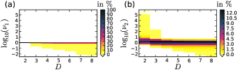
Figure 3: (Color online) Histograms (color-coded) of uncertainties $\nu_{1}$ (a) and $\nu_{2}$ (b) computed from a $x_{1}$ time series of length $N=1000000$ generated on the attractor of the Ikeda map Eq. (11) with reconstruction dimensions ranging from $D=2$ to $D=7$. The state variables $x_{1}$ and $x_{2}$ are estimated ($M=2$) while all parameters are assumed to be known ($K=0$).

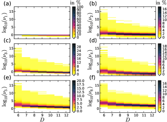
Figure 4: (Color online) Histograms (color-coded) of uncertainties of state and parameter estimates of the Ikeda map Eq. (11) for reconstruction dimensions ranging from $D=6$ to $D=12$. Distributions are computed from a $x_{1}$ time series of length $N=1000000$ generated on the Ikeda attractor. All variables ($M=2$) and all parameters ($K=4$) are assumed to be unknown.

Delay reconstruction can also be applied to observables $s(t)=h[\mathbf{x}(t)]$ from continuous dynamical systems,

$$\mathbf{\dot{x}}=\mathbf{f}(\mathbf{x},\mathbf{p})\,,$$ (12)

using a suitable delay time $\tau$:

$${\mathbf{y}}=\left(s(t),s(t+\tau),....,s(t+(D-1)\tau)\right)=G({\mathbf{x}},\mathbf{p})\in\mathbb{R}^{D}.$$

The Jacobian matrix $DG({\mathbf{x}},\mathbf{p})$ of the delay coordinates map $G$ can be computed by solving linearized equations providing the Jacobian matrices $D_{x}\phi^{t}(\mathbf{x},\mathbf{p})$ and $D_{p}\phi^{t}(\mathbf{x},\mathbf{p})$ of the flow $\phi^{t}$ generated by the system Eq. (12) Kawakami . To demonstrate the application of the proposed uncertainty analysis to continuous time system we use the Hindmarsh-Rose (HR) neuron model HR84

$$\dot{x}_{1} = -x_{1}^{3}+p_{1}x_{1}^{2}+x_{2}-x_{3}$$

$$\dot{x}_{2} = 1-p_{2}x_{1}^{2}-x_{2}$$ (13)

$$\dot{x}_{3} = p_{3}\left(x_{1}+p_{4}(p_{5}-x_{3})\right).$$

For parameter values $p_{1}=3$, $p_{2}=5$, $p_{3}=0.004$, $p_{4}=3.19$, $p_{5}=0.25$ the HR model exhibits chaotic bursting of $x_{1}$ and $x_{2}$ and slow variations of $x_{3}$ SBP11 .

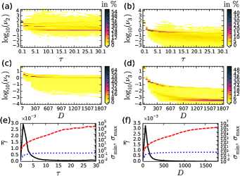
Figure 5: (Color online) Probability distributions (color-coded) of uncertainties $\nu_{2}$ and $\nu_{3}$ when estimating the state variables $x_{1}$, $x_{2}$, and $x_{3}$ of the HR-model Eq. (13) from a $x_{1}$ time series. In (a) and (b) the delay reconstruction dimension is fixed at $D=7$ and the delay $\tau$ is varied. (c), (d) show distributions for $\tau=0.1$ and different reconstruction dimensions $D$. Corresponding columns (histograms) of all four diagrams show results for the same window in time $(D-1)\tau$ used upon delay reconstruction. (e), (f) Observability index $\bar{\gamma}$ (5) (solid curve), $\sigma_{\text{min}}$ (dotted curve), and $\sigma_{\text{max}}$ (dashed curve) vs. $\tau$ and vs. $D$.

Figures 5(a) and 5(b) show the dependence of probability distributions (color-coded) of uncertainties $\nu_{2}$, and $\nu_{3}$, respectively, on the delay time $\tau$ chosen for performing the delay reconstruction. The reconstruction dimension equals $D=7$. With this example, all parameters are assumed to be known ($K=0$) and the first state variable is chosen as measured time series $s(t_{n})=x_{1}(t_{n})$ with $t_{n}=n\tau$. Therefore, the estimation of $x_{1}$ is not much affected by the choice of the delay time and $\nu_{1}\leq 1$ (with $\nu_{1}\approx 1$ most of the time, not shown here). As can be seen the centers of both distributions decrease monotonically with $\tau$ indicating an improvement of the estimation accuracy for larger delay times. Figures 5(c) and 5(d) show histograms (color-coded) of uncertainties $\nu_{2}$, and $\nu_{3}$ versus reconstruction dimension $D$ for $\tau=0.1$. Larger $D$ provides lower uncertainties $\nu_{j}$ and compared to Figs. 5(a) and 5(b) very large $\nu_{j}$ do not occur anymore. Note that corresponding columns of Figs. 5(a) and 5(b) and Figs. 5(c) and 5(d), respectively, are computed using delay coordinates covering the same window in time ranging from $\tau(D-1)=0.1\cdot 6=0.6$ to $\tau(D-1)=30.1\cdot 6=1806\cdot 0.1=180.6$. The more densely sampling ($\tau=0.1$) underlying Figs. 5(c) and 5(d) provides more information about the underlying dynamics and results in lower uncertainty values. Figures 5(e) and 5(f) show the observability index $\bar{\gamma}$ Eq. (5) and mean values of the smallest and the largest singular values $\sigma_{\text{min}}$ and $\sigma_{\text{max}}$ versus $\tau$ and $D$, respectively. While $\bar{\gamma}$ exhibits a clear peak, $\sigma_{\text{min}}$ converges to an asymptotic value, and $\sigma_{\text{max}}$ increases monotonically, i.e., the lengths of the ellipsoid axes in Fig. 1 decrease ($1/\sigma_{\text{max}}$) or converge ($1/\sigma_{\text{min}}$).

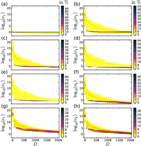
Figure 6: (Color online) Distributions of uncertainties $\nu_{j}$ vs. reconstruction dimension $D$ obtained for the HR model (13) where all three state variables and all five parameters are estimated from a $x_{1}$ time series. The delay time $\tau=0.1$ is fixed.

If in addition to the three state variables $x_{1}$, $x_{2}$, and $x_{3}$ also the five parameters $p_{1},\ldots,p_{5}$ of the HR-model Eq. (13) are to be estimated from the $x_{1}$ time series then we have to cope with an estimation task with $M+K=3+5=8$ uncertainties whose distributions for $\tau=0.1$ are shown in Fig. 6 for delay reconstruction dimensions ranging from $D=8$ to $D=2008$. For increasing $D$ the uncertainties $\nu_{1},\ldots,\nu_{6}$ corresponding to $x_{1},x_{2},x_{3},p_{1},p_{2},p_{3}$ decrease to values close to or below one. The uncertainties $\nu_{7}$ and $\nu_{8}$ of parameters $p_{4}$ and $p_{5}$, respectively, remain rather large ($>1000$) even for high dimensional reconstructions. This feature indicates that it is very difficult to estimate both parameters together. In fact, if $p_{4}$ (or $p_{5}$) is known and only $p_{5}$ (or $p_{4}$) has to be estimated (together with $x_{1},x_{2},x_{3},p_{1},p_{2},p_{3}$) then the uncertainty values of $p_{5}$ (or $p_{4}$) are much smaller and lie in the range of the uncertainties of the other parameters. Applying a state and parameter estimation algorithm SBP11 ; SBLP13 we also encountered problems (in terms of large deviations from the true values) when trying to estimate both parameters $p_{4}$ and $p_{5}$ together. These two parameters are to some degree redundant in the sense that different combinations yield (almost) the same $x_{1}$ time series and thus cannot be clearly distinguished using a $x_{1}$ time series, only.

The presented approach for quantifying uncertainties of model based state and parameter estimation from time series provides a general criterion whether and how reliably specific model variables and parameters can be estimated from time series. This method is independent from any particular estimation method and it can be extended in several ways, including unknown parameters in the measurement function and multivariate time series. High uncertainty implies that the corresponding quantity of the model has small impact on the output and may thus be a candidate for reducing the formal model complexity by pruning. Furthermore, the information provided by the values of uncertainty can be exploited to improve state and parameter estimation methods.

- (1) H. Nijmeijer and I.M.Y. Mareels, IEEE Trans. Circuits Syst. I 44, 882 (1997).
- (2) H.J.C. Huijberts, T. Lilge, and H. Nijmeijer, Int. J. Bif. Chaos 11, 1997 (2001),
- (3) U. Parlitz, L. Junge, and L. Kocarev, Phys. Rev. E 54, 6253 (1996).
- (4) D. Ghosh and S. Banerjee, Phys. Rev. E 78, 056211 (2008).
- (5) H. D. I. Abarbanel, D.R. Creveling, and J.M. Jeanne, Phys. Rev. E 77, 016208 (2008).
- (6) F. Sorrentino and E. Ott, Chaos 19, 033108 (2009).
- (7) P.J. van Leeuwen, Q. J. R. Meteorol. Soc. 136, 1991 (2010).
- (8) H.D.I. Abarbanel, Phys. Lett. A 373, 4044 (2009).
- (9) J.C. Quinn and H.D.I. Abarbanel, Q. J. R. Meteorol. Soc. 136, 1855 (2010).
- (10) D.R. Creveling, P.E. Gill, and H. D. I. Abarbanel, Phys. Lett. A 372, 2640 (2008).
- (11) J. Schumann-Bischoff and U. Parlitz, Phys. Rev. E 84, 056214 (2011).
- (12) J. Bröcker, Q. J. R. Meteorol. Soc. 136, 1906 (2010).
- (13) D. Aeyels, SIAM J. Contr. Optimiz. 19, 595603 (1981).
- (14) F. Takens, Lect. Notes Math. 898, 366 (1981).
- (15) T. Sauer, J.A. Yorke, and M. Casdagli J. of Stat. Phys. 65, 579 (1991).
- (16) H. Kantz and T. Schreiber, Nonlinear Time Series Analysis, Cambridge Nonlinear Science Series 7, (Cambridge University Press, Cambridge, 1997).
- (17) H.D.I. Abarbanel, Analysis of Observed Chaotic Data, (Springer Verlag, 1997), 2nd ed.
- (18) C. Letellier, L.A. Aguirre, and J. Maquet, Phys. Rev. E 71, 066213 (2005); Comm. Nonl. Sci. Num. Sim. 11, 555 (2006).
- (19) C. Letellier and L.A. Aguirre, Phys. Rev. E 79, 066210 (2009).
- (20) M. Frunzete, J.-P. Barbot, and C. Letellier, Phys. Rev. E 86, 026205 (2012).
- (21) R. Hermann and A. J. Krener, IEEE Trans. Autom. Contr. AC-22, 728 (1977).
- (22) E.D. Sontag, Mathematical Control Theory: Deterministic Finite Dimensional Systems, (Springer, New York, 1998) 2nd ed.
- (23) H. Nijmeijer, Int. J. Control 36, 867 (1982).
- (24) H. U. Voss, J. Timmer, and J. Kurths, Int. J. of Bif. and Chaos 14, 1905 (2004).
- (25) K. Ikeda, Opt. Commun. 30, 257 (1979).
- (26) P. Bryant, R. Brown, and H.D.I. Abarbanel, Phys. Rev. Lett. 65, 1523 (1990).
- (27) H. Kawakami, IEEE Trans. Circ. Syst. CAS-31, 248 (1984).
- (28) J. L. Hindmarsh and R. M. Rose, Proc. R. Soc. Lond. B 221, 87 (1984).
- (29) J. Schumann-Bischoff, S. Luther, and U. Parlitz, Commun. Nonlin. Sci. Num. Sim. 18, 2733 (2013).