A Fast Propagation Method
for the Helmholtz equation

Abstract

A fast method is proposed for solving the high frequency Helmholtz equation. The building block of the new fast method is an overlapping source transfer domain decomposition method for layered medium, which is an extension of the source transfer domain decomposition method proposed by Chen and Xiang [4, 5]. The new fast method contains a setup phase and a solving phase. In the setup phase, the computation domain is decomposed hierarchically into many subdomains of different levels, and the mapping from incident traces to field traces on all the subdomains are set up bottom-up. In the solving phase, first on the bottom level, the local problem on the subdomains with restricted source is solved, then the wave propagates on the boundaries of all the subdomains bottom-up, at last the local solutions on all the subdomains are summed up top-down. The total computation cost of the new fast method is $O(n^{\frac{3}{2}}\log n)$ for 2D problem. Numerical experiments shows that with the new fast method, Helmholtz equations with half billion unknowns could be solved efficiently on massively parallel machines.

Key words. Helmholtz equation, fast method, domain decomposition method, PML.

1 Introduction

We consider in this paper to solve the Helmholtz equation in the full space $\mathbb{R}^{2}$, with Sommerfeld radiation condition,

$$\Delta u+k^{2}u =f\qquad\mbox{in}\,\,\,\mathbb{R}^{2},$$ (1)

$$r^{1/2}(\frac{\partial u}{\partial r}-\mathbf{i}ku) \rightarrow 0\qquad\mbox{as}\,\,\,r=|x|\rightarrow\infty$$

where $k$ is the wave number.

Many domain decomposition method has recently been developed to solve the Helmholtz equation, most of them are non-overlapped, and the major differences are the interface conditions. Engquist and Ying [9, 10] proposed a sweeping preconditioner by approximating the inverse of Schur complements in the LDL^t factorization, Stolk [13] proposed a domain decomposition method with a transmission condition based on perfect matched layers, Vion an Geuzaine [14] proposed a double sweep preconditioner that use a transmission condition that involves Dirichlet-to-Neumann (DtN) operator, Zepeda [15] introduced the method of polarized trace that use a transmission condition in boundary integral form, Liu and Ying [12] developed an additive sweeping preconditioner that use a transmission condition built with the boundary values of the intermediate wave directly. Chen and Xiang [4, 5] proposed the source transfer domain decomposition method that transfer the source in subdomains, and recently Du and Wu [8] improved the method so that the transfer applies in both directions.

The domain decomposition method in the literature usually approximately solves the Helmholtz equation with varying medium, either with approximated interface condition or with approximated Green function, thus they are commonly used as preconditioners for Krylov subspace method such as GMRES.

An overlapping source transfer domain decomposition method is proposed for Helmholtz equation with layered medium, the method follows the natural wave traveling process in layered medium, which involves the reflections and refractions at the interface of the layers. The convergence of the new domain decomposition method is ensured by the overlapping region, and the accuracy of the new domain decomposition method makes it the building block of the new fast method.

The domain decomposition method suffers from slow convergence rate when the number of subdomains is large, thus multilevel grid is needed so that the information is brought to far away subdomains without passing the subdomains on the way. The upper level grid for Poisson type problem could be coarser since the amount of information decreases fast as the distance grows. However, for Helmholtz equation, the grid size should be maintained small to represent wave shapes on the upper level grid. Fortunately, the trace on the subdomain boundaries could be used to represent the solution on the subdomain, thus the computation cost on upper level grid is not formidable.

The fast method we proposed first setup the trace mapping on subdomains of different levels. Then the sources are converted to traces on the bottom level, and propagate on higher and higher levels till the top level, then the traces on high levels are decomposed into traces on lower and lower level, at last the traces in the bottom level is converted back to solutions and summed up. In such up and down process, the wave travels to far away regions via the traces on high levels.

The rest of the paper is organized as follows. In section 2, an overlapping source transfer domain decomposition method is proposed for Helmholtz equation with layered medium. In section 3, the fast algorithm is described. The multilevel domain decomposition with quadtree structure is built, and the algorithm to build incident trace to field trace mapping on subdomains is proposed, then source up and solution down algorithm are proposed. The numerical experiment for Marmousi model is present in section 4.

2 The overlapping source transfer DDM

The foundation of the fast method is the overlapping source transfer domain decomposition method for the Helmholtz equation. We first propose and analyze the overlapping STDDM for Helmholtz problem with three layered medium, then revise the method and substitute the solving of subdomain problem into mapping, and at last propose the overlapping decomposition method for four subdomains, which is the building block of the fast propagation method.

2.1 STDDM in three layered medium

Consider the Helmholtz equation (1) defined in $\mathbb{R}^{2}$, where the source $f$ is given, and the wave number $k$ is different in three horizontal layers,

$$k(y)=\left\{\begin{array}[]{ll}k_{1},&\quad\mbox{if ~{} $y<-d$}\\ k_{2},&\quad\mbox{if ~{} $-d\leq y\leq d$}\\ k_{3},&\quad\mbox{if ~{} $y>d$}\\ \end{array}\right.$$ (2)

as shown in Fig 1. The upper interface $y=d$ is denoted $\Gamma_{1}$, and the lower interface $y=-d$ is denoted $\Gamma_{2}$.

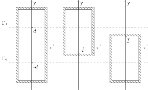
Figure 1: Domain decomposition in $y$ direction for three layered problem.

The frequence domain wave equations defined on unbounded domain could be solved on truncated domain with the perfect matched layer as the absorbing boundary condition [2, 6]. To solve Helmholtz problem (1), the unbounded domain $\mathbb{R}^{2}$ is truncated to a rectangle $[-l_{1},l_{1}]\times[-l_{2},l_{2}]$, with a PML layer of length $l_{\text{pml}}$ attached to the boundary, and the trucated domain $\Omega$ becomes $[-l_{1}-l_{\text{pml}},l_{1}+l_{\text{pml}}]\times[-l_{2}-l_{\text{pml}},l_{2}+l_{\text{pml}}]$. We refer the domain without PML layer as the interior of domain $\Omega$, denoted $\tilde{\Omega}$. For simplicity , we denote $-l_{1}-l_{\text{pml}}$ as $\bar{l}_{1}$.

The uniaxial PML method [6] is used in this paper, where the complex coordinate is streched in $x$ and $y$ direction sperately, $\displaystyle\tilde{x}_{j}(x_{j})=\int_{0}^{x_{j}}\sigma_{j}(t)dt$, $j=1,2$, and the medium perporty is chosen that $\sigma_{j}(t)=0$ for $|t|\leq l_{j}$, and $\sigma_{j}(t)>0$ in PML layer $|t|>l_{j}$. Then the PML equation is

$$J^{-1}\nabla\cdot(A\nabla u)+k^{2}u=f,\qquad\mbox{in}\,\,\,\Omega,$$ (3)

where $\displaystyle A(x)=\mbox{diag}\left(\frac{\alpha_{2}(x_{2})}{\alpha_{1}(x_{1})},\frac{\alpha_{1}(x_{1})}{\alpha_{2}(x_{2})}\right)$, and $J(x)=\alpha_{1}(x_{1})\alpha_{2}(x_{2})$.

The computation domain is decomposed to two overlapping subdomains, the upper one $\Omega_{1}=[-\bar{l}_{1},\bar{l}_{1}]\times[-\tilde{l}-l_{\text{pml}},l_{2}+l_{\text{pml}}]$ and the lower one $\Omega_{2}=[-\bar{l}_{1},\bar{l}_{1}]\times[-l_{2}-l_{\text{pml}},\tilde{l}+l_{\text{pml}}]$, with an overlapping region $[-\bar{l}_{1},\bar{l}_{1}]\times[-\tilde{l},\tilde{l}]$, as is shown in Fig 1. Similar PML equations as (3) are built on the two subdomains, and the parameter $A$ and $J$ in the PML equation are denoted $A_{i}$ and $J_{i}$ for subdomain $\Omega_{i}$, $i=1,2$.

The new domain decomposition method first solve the subdomain problem with the restricted source,

$$J_{i}^{-1}\nabla\cdot(A_{i}\nabla u_{i})+k^{2}u_{i}=f_{i},\qquad\mbox{in}\,\,\,\Omega_{i},i=1,2$$ (4)

where $f_{1}=f\cdot\chi_{y<0}$ for $\Omega_{1}$, and $f_{2}=f\cdot\chi_{y\geq 0}$ for $\Omega_{2}$, and the solution is denoted $u_{i}^{0}$ for $i=1,2$.

Then, the wave field in $\Omega_{1}$ is transfered as source to $\Omega_{2}$ meanwhile the wave field in $\Omega_{2}$ is transfered as source to $\Omega_{1}$, with the new transfered sources the PML equation on the subdomains is solved and new wave field is generated, and so on,

$$J_{1}^{-1}\nabla\cdot(A_{1}\nabla u_{1}^{s+1})+k^{2}u_{1}^{s+1}=\Psi_{1}(u_{2}^{s}), \qquad\mbox{in}\,\,\,\Omega_{1}$$ (5)

$$\Psi_{1}(u_{2}^{s})=-J_{1}^{-1}\nabla\cdot(A_{1}\nabla u_{2}^{s})-k^{2}u_{2}^{s}, \qquad\mbox{in}\,\,\,\Omega_{1}$$

$$J_{2}^{-1}\nabla\cdot(A_{2}\nabla u_{2}^{s+1})+k^{2}u_{2}^{s+1}=\Psi_{2}(u_{1}^{s}), \qquad\mbox{in}\,\,\,\Omega_{2}$$ (6)

$$\Psi_{2}(u_{1}^{s})=-J_{2}^{-1}\nabla\cdot(A_{2}\nabla u_{1}^{s})-k^{2}u_{1}^{s}, \qquad\mbox{in}\,\,\,\Omega_{2}$$

where $\Psi_{1}$ and $\Psi_{2}$ are the source transfer function, $s$ is the iteration step, $s=0,1,2,\ldots$ Note that the transfered source $\Psi_{1}(u_{2}^{s})=0$ for $y<\tilde{l}$ or $y>\tilde{l}+l_{\text{pml}}$ , thus it has a compact support in the PML layer, so does $\Psi_{1}(u_{2}^{s})$. At last, the PML solutions on subdomains are summed up as the solution obtained by the domain decomposition method,

$$u_{\text{DDM}}=\sum_{s=0}^{\infty}(u_{1}^{s}+u_{2}^{s}).$$ (7)

Although the PML equation (4)-(6) sovles the truncated Helmholtz equation in the subdomain approximately, the convergence of the series (7) to the solution of (3) could be shown by

$$\,{\mathscr{L}}\left(\sum_{s=0}^{N}(u_{1}^{s}+u_{2}^{s})\right)-f$$

$$= \,{\mathscr{L}}(u_{1}^{0}+u_{2}^{0})-f+{\mathscr{L}}\left(\sum_{s=1}^{N}(u_{1}^{s}+u_{2}^{s})\right)$$

$$= \,-\Psi(u_{1}^{0})-\Psi(u_{2}^{0})+{\mathscr{L}}(u_{1}^{1}+u_{2}^{1})+{\mathscr{L}}\left(\sum_{s=2}^{N}(u_{1}^{s}+u_{2}^{s})\right)$$

$$= \,-\Psi(u_{1}^{1})-\Psi(u_{2}^{1})+{\mathscr{L}}(u_{1}^{2}+u_{2}^{2})+{\mathscr{L}}\left(\sum_{s=3}^{N}(u_{1}^{s}+u_{2}^{s})\right)$$

$$= \,\ldots$$

$$= \,{\mathscr{L}}(u_{1}^{N}+u_{2}^{N}),$$

and the remaining term ${\mathscr{L}}(u_{1}^{N}+u_{2}^{N})\rightarrow 0$ as $N\rightarrow\infty$, which could be ensured by the convergence of the PML method [3] together with the analysis of wave traveling in layered medium as follows.

The solution of the domain decomposition method in the form of (7) could be interpreted as the superposition of the incident waves, reflected waves and refracted waves that propagate in the layers [7], as is illustrated in Fig 2.

Figure 2: Wave traveling in three layered medium.

Suppose the incident wave $U_{0}$ comes from the upper layer, then at interface $\Gamma_{1}$, $U_{0}$ causes a reflected wave $U_{00}$ going upwards in the upper layer and a refracted wave $U_{01}$ going downwards in the middle layer. The wave $U_{0}+U_{00}+U_{01}$ is approximately the solution $u_{1}^{0}$ of the subdomain equation (4) with $i=1$.

Then at interface $\Gamma_{2}$, $U_{01}$ causes a reflected wave $U_{012}$ going downwards in the lower layer and a refracted wave $U_{011}$ going upwards in the middle layer. The wave $U_{01}+U_{012}+U_{011}$ is approximately the solution $u_{2}^{1}$ of the subdomain equation (6).

Then at interface $\Gamma_{1}$, $U_{011}$ causes a reflected wave $U_{0110}$ going upwards in the upper layer and a refracted wave $U_{0111}$ going downwards in the middle layer. The wave $U_{011}+U_{0110}+U_{0111}$ is approximately the solution $u_{1}^{2}$ of the subdomain equation (5). The traveling process goes on, and the superposition of all the waves is the solution to (3),

$$u =U_{0}+U_{00}+U_{01}+U_{012}+U_{011}$$

$$\quad+U_{0110}+U_{0111}+U_{01112}+U_{01111}+\dots$$ (8)

and the series (2.1) is approximately the series (7).

The convergence of the new overlapping domain decomposition method related closely to the medium perporty of the layers and the size of the overlapping region. When the overlapping region of the subdomains lies inside the middle layer of the three, e.g., $\tilde{l}<d$, the convergence rate of the domain decomposition method is at most the convergence rate of the series (2.1). The worst case happens when there is a narrow wave guide, and the overlapping domain lies inside the wave guide, e.g. $k_{2}>k_{1}=k_{3}$, $\tilde{l}<d$ and $d$ is small. To avoid such cases, the overlapping region should have a non-zero minimum size.

The overlapping region ensures the convergence of the new domain decomposition method for layered medium. The convergence of non-overlaping DDM might deteriorate if the subdomain interface lies right in a waveguide. We have two remarks on the new domain decomposition method.

Remark 1: The convergence of the solution enables direct solving the Helmholtz equation with the method, rather than use it as a preconditioner, which is crucial for our new fast method.

Remark 2: An extend PML layer could be defined that it includes a PML layer and a layer that doesn’t absorb at all, for example, the layer $[-\bar{l}_{1},\bar{l}_{1}]\times[0,\tilde{l}+l_{\text{pml}}]$ is an extend PML layer. Since it’s all about the PML layer parameters, we do not make a distinction between the two and simply call them the PML layer.

2.2 Mapping instead of solving

The domain decomposition method in the above subsection could be revised that the solving of PML equation on subdomains (5)-(6) is substituted by mapping.

For subdomain $\Omega_{1}$, a mapping ${\mathcal{G}}_{1}$ from incidents trace $U^{\text{I}}$ on the line $[-\bar{l}_{1},\bar{l}_{1}]\times 0$ to the wave solution $\bar{u}$ in $\Omega_{1}$ is defined as follows: Given $U^{\text{I}}$ on the line $[-\bar{l}_{1},\bar{l}_{1}]\times 0$, solve $\hat{u}$ as its extension such that

$$J_{2}^{-1}\nabla\cdot(A_{2}\nabla\hat{u})+k^{2}\hat{u}=0, \qquad\mbox{in}\,\,\,[-\bar{l}_{1},\bar{l}_{1}]\times[0,\tilde{l}+l_{\text{pml}}]$$ (9)

$$\hat{u}=U^{\text{I}}, \qquad\mbox{on}\,\,\,[-\bar{l}_{1},\bar{l}_{1}]\times 0$$ (10)

It’s obvious that if $U^{\text{I}}$ is the trace of a solution to (6), then $\hat{u}$ is the restriction of that solution on the region $[-\bar{l}_{1},\bar{l}_{1}]\times[0,\tilde{l}+l_{\text{pml}}]$. The extension $\hat{u}$ is then transfered as source,

$$\Psi_{1}(\hat{u})=-J_{1}^{-1}\nabla\cdot(A_{1}\nabla\hat{u})-k^{2}\hat{u},\qquad\mbox{in}\,\,\,\Omega_{1},$$ (11)

with which the wave field solution $\bar{u}$ to PML equation in subomain $\Omega_{1}$ is solved

$$J_{1}^{-1}\nabla\cdot(A_{1}\nabla\bar{u})+k^{2}\bar{u}=\Psi_{1}(\hat{u}),\qquad\mbox{in}\,\,\,\Omega_{1}.$$ (12)

The mapping is then defined as $\bar{u}={\mathcal{G}}_{1}(U^{\text{I}})$.

Another mapping ${\mathcal{F}}_{1}$ from incidents trace $U^{\text{I}}$ on the line $[-\bar{l}_{1},\bar{l}_{1}]\times 0$ to the field trace $U^{\text{F}}$ on the same line, is defined by $\displaystyle U^{\text{F}}={\mathcal{F}}_{1}(U^{\text{I}})\triangleq\left.{\mathcal{G}}_{1}(U^{\text{I}})\right|_{[-\bar{l}_{1},\bar{l}_{1}]\times 0}$ . Although both the incident trace and the field trace is on the line $[-\bar{l}_{1},\bar{l}_{1}]\times 0$ , it is referred as incident boundary or field boundary, respectfully. For subdomain $\Omega_{2}$, similar mapping ${\mathcal{G}}_{2}$ and ${\mathcal{F}}_{2}$ could be defined.

Now the domain decomposition method for Helmholtz equation with three layered medium could be revised as follows: first, solve the subdomain problem with the restricted source,

$$J_{i}^{-1}\nabla\cdot(A_{i}\nabla u_{i})+k^{2}u_{i}=f_{i},\qquad\mbox{in}\,\,\,\Omega_{i},i=1,2$$ (13)

where $f_{1}=f\cdot\chi_{y<0}$ for $\Omega_{1}$, and $f_{2}=f\cdot\chi_{y\geq 0}$ for $\Omega_{2}$, the solution is denoted $u_{i}^{0}$ for $i=1,2$, and the field trace of the solutions are $U_{i}^{\text{F},0}=\left.u_{i}^{0}\right|_{[-\bar{l}_{1},\bar{l}_{1}]\times 0}$, for $i=1,2$.

Then each subdomain takes its neighbor’s field trace as its own incident trace, map the incident trace to filed trace, and so on,

$$U_{1}^{\text{I},s+1} =U_{2}^{\text{F},s} \qquad\mbox{in}\,\,\,\Omega_{1}$$

$$U_{1}^{\text{F},s+1} ={\mathcal{F}}_{1}(U_{1}^{\text{I},s+1}) \qquad\mbox{in}\,\,\,\Omega_{1}$$

$$U_{2}^{\text{I},s+1} =U_{1}^{\text{F},s} \qquad\mbox{in}\,\,\,\Omega_{2}$$

$$U_{2}^{\text{F},s+1} ={\mathcal{F}}_{2}(U_{2}^{\text{I},s+1}) \qquad\mbox{in}\,\,\,\Omega_{2}$$

for $s=0,1,2,\ldots$, and the domain decomposition solution is

$$u_{\text{DDM}}=u_{1}+u_{2}+{\mathcal{G}}_{1}\left(\sum_{k=0}^{\infty}U_{1}^{\text{I},s}\right)+{\mathcal{G}}_{2}\left(\sum_{s=0}^{\infty}U_{2}^{\text{I},s}\right).$$ (15)

2.3 STDDM with four subdomains

The above domain decomposition method with two subdomain in $y$ direction could be easily extended to four subdomains in both $x$ and $y$ directions. The major difference is that the incident boundaries, field boundaries and their source tranfer regions are a little complicated for four subdomains.

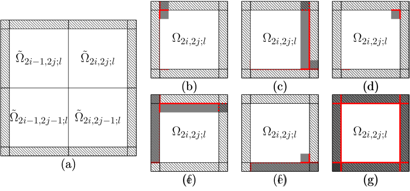
Figure 3: Domain decomposition with four subdomains. The hatched area is the PML layer, the shaddowed area is the source transfer region, the thick lines are the incident or field boundaries. (a) four subdomain’s interior region $\tilde{\Omega}_{i,j}$, $i,j=1,2$ and the PML layer of total domain. (b-d) incident boundaries and corresponding source transfer region of subdomain $\Omega_{2,2}$. (e-g) field boundaries and corresponding source transfer region of subdomain $\Omega_{2,2}$.

The total domain $\Omega$ is decomposed into four smaller subdomains $\Omega_{i,j}$, $i,j=1,2$. The interior (region without PML layer) of the subdomain $\Omega_{i,j}$ are denoted $\tilde{\Omega}_{i,j}$, they are non-overlapped and their union is the interior of the total domain, as is shown in Fig 3 -(a). Each subdomain $\Omega_{i,j}$ has its PML layer lie in its neighbors.

There are three kind of incident boundaries, denoted $\Gamma_{i,j}^{\text{I}}$, and three kind of field boundaries, denoted $\Gamma_{i,j}^{\text{F}}$, for subdomain $\Omega_{i,j}$, as in Fig 3 -(b-g). For examples, on subdomain $\Omega_{2,2}$, the incident boundary for wave comes from subdomain $\Omega_{1,2}$ is shown in Fig 3 -(b), and the field boundary for wave goes to subdomain $\Omega_{1,2}$ is shown in Fig 3 -(e).

The incident traces on boundary $\Gamma_{i,j}^{\text{I}}$ are denoted as $U_{i,j}^{\text{I}}$, and the field traces on boundary $\Gamma_{i,j}^{\text{F}}$ are denoted as $U_{i,j}^{\text{F}}$. The mapping from the incident trace to the solution on subdomain $\Omega_{i,j}$ is denoted ${\mathcal{G}}_{i,j}$, while the the mapping from the incident trace to the field trace on subdomain $\Omega_{i,j}$ is denoted ${\mathcal{F}}_{i,j}$

The domain decomposition method with four subdomains is shown in Algorithm 2.3. In the algorithm, the wave propagates between children subdomains via the iteration (3 -7), we call it the iteration of incident and field traces from now on.

  Algorithm 1 Domain decomposition with four subdomains.

 

1:Solve the mapping ${\mathcal{F}}_{i,j}$ on subdomain $\Omega_{i,j}$, $i,j=1,2$,

2:     with direct solver.

3:Solve the local problem on $\Omega_{i,j}$ with source $f_{i,j}=f|\tilde{\Omega}_{i,j}$,

4:     restrict the solution $u_{i,j}^{0}$ to field trace $U_{i,j}^{\text{F},0}$.

5:while $\sum_{i,j=1,2}||U_{i,j}^{\text{F},s}||>\varepsilon$ do

6:     Send subdomain $\Omega_{i,j}$’s field trace $U_{i,j}^{\text{F},s}$

7:              to its siblings $\Omega_{i^{\prime},j^{\prime}}$ as incident trace $U_{i^{\prime},j^{\prime}}^{\text{I},s+1}$

8:     Record the incident traces $U_{i,j}^{\text{I},s+1}$

9:     Map the incidents trace to field trace $U_{i,j}^{\text{F},s+1}={\mathcal{F}}_{i,j}(U_{i,j}^{\text{I},s+1})$

10:     Set $s=s+1$

11:end while

12:Solve the local problem on $\Omega_{i,j}$ with the summation of incident traces using direct solver, the solution is denoted ${\mathcal{G}}_{i,j}\left(\sum_{s>0}U_{i,j}^{\text{I},s}\right)$.

13:Sum up the solutions of all subdomains to get the total solution

$$u=\sum_{i,j=1,2}\left(u_{i,j}^{0}+{\mathcal{G}}_{i,j}\left(\sum_{s>0}U_{i,j}^{\text{I},s}\right)\right).$$

 

3 The Fast Propagation Method

3.1 Hierarchical domain decomposition

Figure 4: Hierarchical Domain decomposition with 4 levels. From left to right, domain decomposition on level 1, 2, 3, 4.

A rectangular domain of $[-L,L]$ is decomposed into smaller rectangular blocks (or subdomain) on different levels. Denote the number of levels as $N_{L}+1$, the level $l=0$ is referred as the bottom level and the level $l=N_{L}$ is referred as the top level. The number of blocks in $x$ direction at level $l$ is $2^{N_{L}-l}$, where $l=0,\ldots,N_{L}$. Let $I_{l}=\left\{1,\ldots,2^{N_{L}-l}\right\}$, on the level $l$, the block which is the $i$-th block in $x$ direction and the $j$-th block in $y$ direction, is denoted $\Omega_{i,j;l}$, where $i,j\in I_{l}$. Each block shares an overlapping PML layer region of length $l_{\text{pml}}$ with its neighbors on the same level.

The quadtree structure of the multiple level domain decomposition is built as follows. Each block $\Omega_{i,j;l}$ on level $l=2^{N_{L}-l},\dots,1$ has four children $\displaystyle\Omega_{2i-1,2j-1;\,l-1}$, $\displaystyle\Omega_{2i-1,2j;\,l-1}$, $\displaystyle\Omega_{2i,2j-1;\,l-1}$, and $\displaystyle\Omega_{2i,2j;\,l-1}$ on level $l-1$. For simplicity, the children of block $\Omega_{i,j;\,l}$ is denoted $\Omega_{i^{\prime},j^{\prime};\,l-1}$, where $i^{\prime}=2i-1,2i$, $j^{\prime}=2j-1,2j$. On the other hand, each block $\displaystyle\Omega_{i,j;\,l}$ on level $l$ has a father $\displaystyle\Omega_{\lceil i/2\rceil,\lceil j/2\rceil;\,l+1}$ on level $l+1$, where $l<N_{L}$. The father-son relationship of the blocks leads to the quadtree structure.

The incident boundaries and field boundaries on block $\Omega_{i,j;\,l}$ include not only the boundaries between siblings as in Fig 3, but also its ascendant’s incident boundaries and field boundaries, as is shown in Fig 5. We call the boundaries as in Fig 3 the corresponding incident and field boundaries between siblings. The incident boundary of block $\Omega_{i,j;\,l}$ is denoted $\Gamma_{i,j;\,l}^{\text{I}}$, and the field boundary of block $\Omega_{i,j;\,l}$ is denoted $\Gamma_{i,j;\,l}^{\text{F}}$. We see $\displaystyle\Gamma_{i,j;l}^{\text{I}}\subset\mathop{\cup}_{i^{\prime},j^{\prime}}\Gamma_{i^{\prime},j^{\prime};l-1}^{\text{I}}$ and $\displaystyle\Gamma_{i,j;l}^{\text{F}}\subset\mathop{\cup}_{i^{\prime},j^{\prime}}\Gamma_{i^{\prime},j^{\prime};l-1}^{\text{F}}$. The mapping from incident trace to solution on the block is denoted ${\mathcal{G}}_{i,j;l}$, and the mapping from incident trace to field trace on the block is denoted ${\mathcal{F}}_{i,j;l}$ .

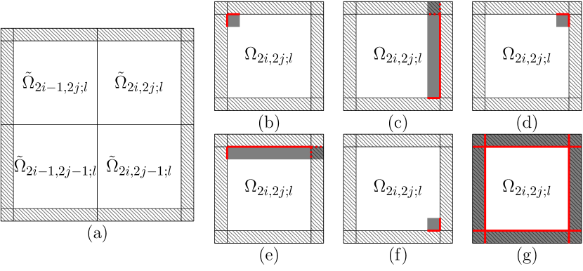
Figure 5: Incident boundaries and field boundaries extension. The hatched area is the PML layer, the shaddowed area is the source transfer region, the thick lines are the incident or field boundaries. (a) four children block’s interior region and the PML layer of father block $\Omega_{i,j;\,l+1}$. (b-f) ascendant’s incident boundaries and corresponding source transfer region on child $\Omega_{2i,2j;\,l}$. (e) total field traces and corresponding source transfer region on child $\Omega_{2i,2j;\,l}$.

3.2 Setup phase

In the setup phase, the mapping from incident traces to field traces is constructed bottom up level by level. The mapping on block $\Omega_{i,j}^{\,0}$, $i,j\in I_{0}$ could be computed with external direct solver, and the mapping on block $\Omega_{i,j;\,l}$ of level $l>0$ is computed as follows.

Given an incident $\delta$ lies in $\Gamma_{i,j;\,l}^{\text{I}}$ , it must lie in the incident boundary of one of the children, denoted as $\Omega_{i_{0},j_{0};\,l-1}$. First the local problem on children $\Omega_{i_{0},j_{0};\,l-1}$ with source $\delta$ is considered, and the field trace of the solution on $\Gamma_{i_{0},j_{0};\,l-1}^{\text{F}}$ is solved by mapping ${\mathcal{F}}_{i_{0},j_{0};\,l-1}$. Then the field trace of $\Omega_{i_{0},j_{0};\,l-1}$ is send to its siblings as incidents, and the iteration of incident and filed trace between siblings applies, and the incident trace in the iteration is denoted $U_{i^{\prime},j^{\prime};\,l-1}^{\text{I},s}$, where $s$ is the iteration number. At last, field trace on $\Gamma_{i^{\prime},j^{\prime};\,l-1}^{\text{F}}$ caused by sum of incidents computed with the mapping ${\mathcal{F}}_{i^{\prime},j^{\prime};\,l-1}$, along with the field trace caused by $\delta$ on $\Omega_{i_{0},j_{0};\,l-1}$, are add up as the field trace $U_{i,j;\,l}^{\text{F}}$ on $\Omega_{i,j;\,l}$ caused by $\delta$,

$$U_{i,j;\,l}^{\text{F}}={\mathcal{F}}_{i_{0},j_{0};\,l-1}(\delta)\Big{|}_{\Gamma_{i,j;\,l}^{\text{F}}}+\sum_{i^{\prime},j^{\prime}}{\mathcal{F}}_{i^{\prime},j^{\prime};\,l-1}(\sum_{s}U_{i^{\prime},j^{\prime};\,l-1}^{\text{I},s})\Big{|}_{\Gamma_{i,j;\,l}^{\text{F}}},$$ (16)

and the mapping is

$${\mathcal{F}}_{i,j;\,l}(\delta)=U_{i,j;\,l}^{\text{F}}.$$ (17)

The algorithm of building the mapping from incident traces to field traces is as follows.

  Algorithm 2 Build mapping of incident traces to field traces

 

1:On level 0, build the mapping of incident to field with direct solver.

2:for levels $l=1,\ldots,N_{L}$ do

3:     On block $\Omega_{i,j;\,l}$,

4:     for incident $\delta$ lies in $\Gamma_{i,j;\,l}^{\text{I}}$  do

5:         Find the children $\Omega_{i_{0},j_{0};\,l-1}$ such that $\delta$ lies in $\Gamma_{i_{0},j_{0};\,l-1}^{\text{I}}$

6:         On children $\Omega_{i_{0},j_{0};\,l-1}$,

7:              map the incidents $\delta$ to field trace $U_{i_{0},j_{0};\,l-1}^{\text{F}}$,

8:              and add part of them to father’s field trace $U_{i,j;\,l}^{\text{F}}$.

9:         Set $U_{i_{0},j_{0};\,l-1}^{\text{F},0}=U_{i_{0},j_{0};\,l-1}^{\text{F}}$ on children $\Omega_{i_{0},j_{0};\,l-1}$,

10:              and set $U_{i^{\prime},j^{\prime};\,l-1}^{\text{F},0}=0$ on other children $\Omega_{i^{\prime},j^{\prime};\,l-1}$.

11:         while $\sum_{i^{\prime},j^{\prime}}||U_{i^{\prime},j^{\prime};\,l-1}^{\text{F},s}||>\varepsilon$ do

12:              Send the children’s corresponding field trace $U_{i^{\prime},j^{\prime};\,l-1}^{\text{F},s}$

13:                  to its sibilings as incidens $U_{i^{\prime},j^{\prime};\,l-1}^{\text{I},s+1}$

14:              Map the incidents to field trace $U_{i^{\prime},j^{\prime};\,l-1}^{\text{F},s+1}={\mathcal{F}}_{i^{\prime},j^{\prime};\,l-1}(U_{i^{\prime},j^{\prime};\,l-1}^{\text{I},s+1})$

15:              Set $s=s+1$

16:         end while

17:         Map the sum of incidents to field trace on children,

18:              and add them to father’s field $U_{i,j;\,l}^{\text{F}}$.

19:     end for

20:end for

 

3.3 Solve phase

With the mapping of incident traces to filed traces that is constructed on each block of all levels, the Helmholtz equation could be solved in two phases, the source-up phase and the the solution-down phase.

3.3.1 The Source-up phase

In the source-up phase, the wave propagates on all levels bottom up as incident traces.

The following problem is considered, for the block $\Omega_{i,j;\,l}$, the local solution on its four children are known, e.g., $u_{i^{\prime},j^{\prime};\,l-1}^{0}$, so does their field traces $U_{i^{\prime},j^{\prime};\,l-1}^{\text{F},0}$, how to solve the solution $u_{i,j;\,l}$ on $\Omega_{i,j;\,l}$, and its field trace $U_{i,j;\,l}^{\text{F}}$. The iteration of incident and filed trace between siblings applies directly, denote the incident traces in the iteration as $U_{i^{\prime},j^{\prime};\,l-1}^{\text{I},s}$, and the solution on $\Omega_{i,j;\,l}$ is

$$u_{i,j;\,l}=\sum_{i^{\prime},j^{\prime}}\left(u_{i^{\prime},j^{\prime};\,l-1}^{0}+{\mathcal{G}}_{i^{\prime},j^{\prime};\,l-1}(\sum_{s}U_{i^{\prime},j^{\prime};\,l-1}^{\text{I},s})\right),$$ (18)

and the the field trace of $u_{i,j}^{l}$ is

$$\displaystyle U_{i,j;\,l}^{\text{F}} =\sum_{i^{\prime},j^{\prime}}\left(U_{i^{\prime},j^{\prime};\,l-1}^{\text{F},0}\Big{|}_{\Gamma_{i,j;\,l}^{\text{F}}}+{\mathcal{F}}_{i^{\prime},j^{\prime};\,l-1}(\sum_{s}U_{i^{\prime},j^{\prime};\,l-1}^{\text{I},s})\Big{|}_{\Gamma_{i,j;\,l}^{\text{F}}}\right).$$ (19)

Review the procedure we found that to apply the procedure to next level, the incident to field mapping operation ${\mathcal{F}}_{i^{\prime},j^{\prime};\,l-1}$ of children is needed, while the solving operation ${\mathcal{G}}_{i^{\prime},j^{\prime};\,l-1}(\sum_{s}U_{i^{\prime},j^{\prime};\,l-1}^{\text{I},s})$ could be post processed. Apply the procedure from bottom level to top level leads to the following source-up algorithm.

  Algorithm 3 Source-up

 

1:Right hand side $f$ of the linear system

2:Solution $u_{i,j,0}^{0}$ on $\Omega_{i,j}^{0}$,

3:     and sum of incidents on $\Omega_{i,j;\,l}$ on level $l>0$

4:On level $l=0$,

5:     solve the local problem on $\Omega_{i,j}^{0}$ with the source $f_{i,j}^{0}=f|\hat{\Omega}_{i,j}^{0}$,

6:     the solution $u_{i,j,0}^{0}$ and the its field trace $U_{i,j,0}^{\text{F}}$ are recored.

7:for levels $l=1,\ldots,N_{L}$ do

8:     On block $\Omega_{i,j;\,l}$,

9:         use the field trace $U_{i^{\prime},j^{\prime};\,l-1}^{\text{F}}$ of the four childrens $\Omega_{i^{\prime},j^{\prime};\,l-1}$,

10:         add part of $U_{i^{\prime},j^{\prime};\,l-1}^{\text{F}}$ to $U_{i,j;\,l}^{\text{F}}$,

11:         set $U_{i^{\prime},j^{\prime};\,l-1}^{\text{F},0}=U_{i^{\prime},j^{\prime};\,l-1}^{\text{F}}$,

12:     while $||U_{i^{\prime},j^{\prime};\,l-1}^{\text{F},s}||>\varepsilon$ do

13:         Send children’s corresponding field traces $U_{i^{\prime},j^{\prime};\,l-1}^{\text{F},s}$

14:              to its sibilings as incidens $U_{i^{\prime},j^{\prime};\,l-1}^{\text{I},s+1}$

15:         Map the incidents to field $U_{i^{\prime},j^{\prime};\,l-1}^{\text{F},s+1}={\mathcal{F}}_{i^{\prime},j^{\prime};\,l-1}(U_{i^{\prime},j^{\prime};\,l-1}^{\text{I},s+1})$

16:         Set $s=s+1$

17:     end while

18:     Sum up the incidents $\sum_{s}U_{i^{\prime},j^{\prime};\,l-1}^{\text{I},s}$ for childrens

19:         and map them to the field trace $\Omega_{i,j;\,l}$,

20:         then add to $U_{i,j;\,l}^{\text{F}}$.

21:end for

 

The solution to the total problem could then be expressed as

$$u=\sum_{i,j\in I_{0}}u_{i,j;0}^{0}+\sum_{l>0}\sum_{i,j\in I_{l}}\sum_{i^{\prime},j^{\prime}}\left({\mathcal{G}}_{i^{\prime},j^{\prime};\,l-1}(\sum_{s}U_{i^{\prime},j^{\prime};\,l-1}^{\text{I},s})\right).$$ (20)

3.3.2 The Solution-down phase

In the solution-down phase the wave propagates on all levels top down as incident traces.

The solution (20) resulting from Algorithm 3.3.1 still needs to solve the local Helmholtz problem with given incidents on blocks of different levels, fortunately, the local solutions could be break down to lower and lower level till level 0. We consider the following problem: on the block $\Omega_{i,j;\,l}$, given the incidents ${\tilde{U}}_{i,j;\,l}^{\text{I}}$, how to solve ${\mathcal{G}}_{i,j;\,l}({\tilde{U}}_{i,j;\,l}^{\text{I}})$.

First the incident traces ${\tilde{U}}_{i,j;\,l}^{\text{I}}$ is divided into the incident traces on children ${\tilde{U}}_{i,j;\,l}^{\text{I}}=\displaystyle\sum_{i^{\prime},j^{\prime}}{\tilde{U}}_{i,j;\,l-1}^{\text{I},0}$, then with the incident to field mapping ${\mathcal{F}}_{i^{\prime},j^{\prime};\,l-1}$ on each children, field trace of children is generated, e.g., ${\tilde{U}}_{i^{\prime},j^{\prime};\,l-1}^{\text{F},0}$, then the iteration of incident and filed trace between siblings applies, and the incident traces in the iteration is denoted as $\tilde{U}_{i^{\prime},j^{\prime};\,l-1}^{\text{I},s}$. At last the solution on $\Omega_{i,j;\,l}$ is

$${\mathcal{G}}_{i,j;\,l}({\tilde{U}}_{i,j;\,l}^{\text{I}})=\sum_{i^{\prime},j^{\prime}}\left({\mathcal{G}}_{i^{\prime},j^{\prime};\,l-1}(\sum_{s}{\tilde{U}}^{\text{I},s}_{i^{\prime},j^{\prime};\,l-1})\right)$$ (21)

Apply the procedure from level $l=N_{L}$ to $l=1$, since there are already sum of incidents $\sum_{s}U^{\text{I},s}_{i^{\prime},j^{\prime};\,l-1}$ on children blocks $\Omega_{i^{\prime},j^{\prime};\,l-1}$, the incidents $\sum_{s}{\tilde{U}}^{\text{I},s}_{i^{\prime},j^{\prime};\,l-1}$ from $\Omega_{i,j;\,l}$ should be added on children. The algoritm is discribed as follows.

  Algorithm 4 Solution down

 

1:Solution $u_{i,j;1}^{0}$ on $\Omega_{i,j;1}$,

2:     and sum of incidents on $\Omega_{i,j;\,l}$ on level $l>1$

3:Solution $u$ of the linear system

4:for levels $l=N_{L},\ldots,1$ do

5:     On block $\Omega_{i,j;\,l}$, divide the sum of incidents to its children,

$$\tilde{U}_{i,j;\,l}^{\text{I}}=\displaystyle\sum_{i^{\prime},j^{\prime}}{\tilde{U}}_{i^{\prime},j^{\prime};\,l-1}^{\text{I},0}$$

6:     Map the incidents to field ${\tilde{U}}_{i^{\prime},j^{\prime};\,l-1}^{\text{F},1}={\mathcal{F}}_{i^{\prime},j^{\prime};\,l-1}({\tilde{U}}_{i^{\prime},j^{\prime};\,l-1}^{\text{I},0})$

7:     while $||\tilde{U}_{i^{\prime},j^{\prime};\,l-1}^{\text{I},s}||>\varepsilon$ do

8:         Send children’s corresponding field trace ${\tilde{U}}_{i^{\prime},j^{\prime};\,l-1}^{\text{F},s}$

9:              to its siblings as incidents ${\tilde{U}}_{i^{\prime},j^{\prime};\,l-1}^{\text{I},s+1}$

10:         Map the incidents to field ${\tilde{U}}_{i^{\prime},j^{\prime};\,l-1}^{\text{F},s+1}={\mathcal{F}}_{i^{\prime},j^{\prime};\,l-1}({\tilde{U}}_{i^{\prime},j^{\prime};\,l-1}^{\text{I},s+1})$

11:         Set $s=s+1$

12:     end while

13:     Add the sum of incidents on children $\Omega_{i^{\prime},j^{\prime};\,l-1}$,

$$\tilde{U}_{i^{\prime},j^{\prime};\,l-1}^{\text{I}}:=\sum_{s}U_{i^{\prime},j^{\prime};\,l-1}^{\text{I},s}+\sum_{s}{\tilde{U}}_{i^{\prime},j^{\prime};\,l-1}^{\text{I},s}$$

14:end for

15:On level $l=0$,

16:     solve the local problem on $\Omega_{i,j}^{0}$ with the incidents $\tilde{U}_{i,j;0}^{\text{I}}$,

17:     and add the solution to total solution $u$.

 

Now the solution to the total problem is

$$u=\sum_{i,j\in I_{0}}\left(u_{i,j;0}^{0}+{\mathcal{G}}_{i,j;0}(\sum_{s}\tilde{U}_{i,j;\,0}^{\text{I},s})\right).$$ (22)

4 Numerical experiments

The new method is tested on the 2D Marmousi model in seismology, which is $3,000$ m deep and $9,200$ m wide. Only P-wave is considered, thus elastic wave equation becomes an acoustic equation. The velocity profile is shown in Fig 6, the maximum velocity is 5500 km/s and the minmum velocity is 1500 km/s.

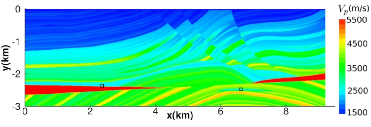
Figure 6: Velocity profile of Marmousi model. The solution with $N_{L}=5$ is sampled in two small boxes in the figure.

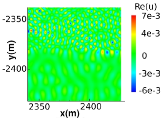
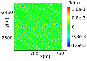
Figure 7: Real part of the solution with $N_{L}=5$ in two small boxes as marked in Fig 6.

Finite difference method with second order of accuracy is used to discretize the Helmholtz equation. The block size on bottom level is 400 $\times$ 400, ant the PML layer is of 40 grid points width. Single shot in the corner of the domain at $(400h_{x},400h_{y})$ is taken as the source, where $h_{x}$, $h_{y}$ are the grid size in $x$ and $y$ direction, respectfully. The shape of the shot is an approximate delta function, $\displaystyle f_{i,j}=\frac{1}{h_{x}h_{y}}\delta(i-400h_{x},j-400h_{y})$.

$N_{L}$	Size	Freq	No.	Time	Time	Time
		$\omega/2\pi$	procs	setup	solve	total
1	2,400 $\times$ 800	37	12	40	195	235
2	4,800 $\times$ 1,600	70	48	140	205	345
3	9,600 $\times$ 3,200	137	192	333	309	642
4	19,200 $\times$ 6,400	270	768	1212	685	1897
5	38,400 $\times$ 12,800	537	3,072	2891	883	3774

Table 1: Time cost (in seconds) of the new method.

$N_{L}$	Time	Time	Time	Time	Time
	Level 0	Level 1	Level 2	Level 3	Level 4
1	39.6	-	-	-	-
2	100	40.1	-	-	-
3	119	86.2	128	-	-
4	127	74.7	256	754	-
5	129	98.7	355	716	1592

Table 2: Detailed setup phase time cost (in seconds).

The fast propagation method is suitable for parallel computing, and could be easily extend to thousands of cores. We test the method with different grid levels and grid sizes on cluster, as listed in Table 1. The tolerance of residual $\displaystyle\frac{||Ax-b||_{2}}{||b||_{2}}$ is $10^{-7}$. Fig 7 shows the solution with $N_{L}=5$ in two small boxes of $400\times 400$ grid points as marked in Fig 6.

The time cost of solving Helmholtz equation with the fast method in parallel is shown in Table 1. The setup phase is the most demanding part in solving, since its complexity is $O(N^{3/2}\log N)$. The detailed time cost in setup phase is shown in Table 2. The mapping on the bottom block is solved with direct solver, e.g. MUMPS [1], and the time cost is almost constant, since the bottom level block is of fixed size. However, the time cost of building mapping on level $l+1$ is roughly twice of level $l$, where $l>0$, which is time consuming for large Helmholtz problems.

5 Conclusions

A fast method is proposed for solving Helmholtz equations, the new method has a setup phase of complexity $O(N^{3/2}\log N)$ and a solve phase of complexity $O(N\log N)$. Our future work is to reduce the computation time of the new method by exploiting the low rank structure of the mappings and accelerating dense matrix operations with GPU.

References

• [1] P. R. Amestoy, I. S. Duff, J. Koster, and J.-Y. L’Excellent. A fully asynchronous multifrontal solver using distributed dynamic scheduling. SIAM Journal on Matrix Analysis and Applications, 23(1):15–41, 2001.
• [2] J.-P. Berenger. A perfectly matched layer for the absorption of electromagnetic waves. J. Comput. Phys., 114(2):185–200, 1994.
• [3] Z. Chen and W. Zheng. Convergence of the uniaxial perfectly matched layer method for time-harmonic scattering problems in two-layered media. SIAM J. Numer. Anal, 48, 2158-2185, 2010.
• [4] Z. Chen and X. Xiang. A source transfer domain decomposition method for Helmholtz equations in unbounded domain. SIAM J. Numer. Anal., 51(4):2331–2356, 2013.
• [5] Z. Chen and X. Xiang. A source transfer domain decomposition method for Helmholtz equations in unbounded domain Part II: Extensions. Numer. Math. Theory Methods Appl., 6(3):538–555, 2013.
• [6] W. C. Chew and W. H. Weedon. A 3D perfectly matched medium from modified Maxwell’s equations with stretched coordinates. Microw. Opt. Techn. Let., 7(13):599–604, 1994.
• [7] W. C. Chew. Waves and Fields in Inhomogenous Media Paperback. Wiley-IEEE Press, February 2, 1999.
• [8] Y. Du and H. Wu. An improved pure source transfer domain decomposition method for Helmholtz equations in unbounded domain. ArXiv e-prints, May. 2015.
• [9] B. Engquist and L. Ying. Sweeping preconditioner for the Helmholtz equation: hierarchical matrix representation. Comm. Pure Appl. Math., 64(5):697–735, 2011.
• [10] B. Engquist and L. Ying. Sweeping preconditioner for the Helmholtz equation: moving perfectly matched layers. Multiscale Model. Simul., 9(2):686–710, 2011.
• [11] M. J. Gander and F. Nataf. AILU for Helmholtz problems: a new preconditioner based on the analytic parabolic factorization. J. Comput. Acoust., 9(4):1499–1506, 2001
• [12] F. Liu and L. Ying. Additive Sweeping Preconditioner for the Helmholtz Equation. ArXiv e-prints, Apr. 2015.
• [13] C. C. Stolk. A rapidly converging domain decomposition method for the Helmholtz equation. J. Comput. Phys., 241(0):240 – 252, 2013.
• [14] A. Vion and C. Geuzaine. Double sweep preconditioner for optimized schwarz methods applied to the Helmholtz problem. J. Comput. Phys., 266(0):171 – 190, 2014.
• [15] L. Zepeda-NΓΊΓ±nez and L. Demanet. The method of polarized traces for the 2D Helmholtz equation. ArXiv e-prints, Oct. 2014.