Phase transition of two-dimensional Ising models on the honeycomb and related lattices with striped random impurities

Abstract

Two-dimensional Ising models on the honeycomb lattice and the square lattice with striped random impurities are studied to obtain their phase diagrams. Assuming bimodal distributions of the random impurities where all the non-zero couplings have the same magnitude, exact critical values for the fraction $p$ of ferromagnetic bonds at the zero-temperature ($T=0$) are obtained. The critical lines in the $p-T$ plane are drawn by numerically evaluating the Lyapunov exponent of random matrix products.

1 Introduction

Ising models have attracted a particular attention in the statistical physics as simplest models that exhibit phase transitions and critical phenomena. The most popular is the pure Ising ferromagnet model on the square lattice, for which not only the transition temperature [18] but also the free energy have been obtained exactly [16, 21]. The hexagonal (honeycomb) lattice is the secondly simplest two-dimensional lattice. The pure Ising model on the honeycomb lattice has been studied by Wannier [28] and Houtapel [11] and exactly solved. Apart from the Ising model, quantum spin models such as the Kitaev model [17] or Kitaev-Heisenberg model [3, 13] on the honeycomb lattice have recently received a lot of theoretical and experimental attentions [4, 5, 23, 26, 30]. Such a growing interest in the honeycomb-lattice systems motivates us to revisit the Ising model on the honeycomb lattice.

In contrast to pure models, less is understood for disordered Ising models. The exact free energy has not been obtained in fully random Ising models in two dimension. Although the transition temperature and/or phase diagram have been investigated using the replica trick, few is revealed so far. Domany showed for the diluted Ising model on the square lattice with concentration $p$ of the ferromagnetic bonds that the zero-temperature phase transition occurs at $p_{c}=1/2$ [6]. Fisch [7], Schwartz [24], and Aharony and Stephen [1] obtained equations to determine the transition temperature for square-lattice models with random interactions each of which takes $J_{1}$ or $J_{2}$ with the same probability.

The problem is simpler if the disorder or impurity exists only in one direction and the system maintains the translational invariance in the other direction. Let us consider an Ising model on the square lattice. Suppose that $J_{ij}^{\rm v}$ and $J_{ij}^{\rm h}$ denote coupling constants on a vertical and a horizontal bonds respectively. McCoy and Wu [20] introduced a model where $J_{ij}^{\rm h}$’s are constant and $J_{ij}^{\rm v}$’s are uniform among the columns but row-to-row random. See Fig. 1. Shankar and Murthy [25] considered a slightly different model, where $J_{ij}^{\rm h}$’s are uniform among a row but row-to-row random while $J_{ij}^{\rm v}$’s are uniform in the whole system (Fig. 1). The criticality condition for both the models was derived in Refs. [29, 15]. It is important that the partition function of the McCoy-Wu and the Shankar-Murthy models can be written as the largest eigenvalue, or the Lyapunov exponent in other words, of a product of random $2\times 2$ matrices. As far as the transition temperature is concerned, however, it is sufficient to work with random diagonal matrices.

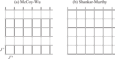
Figure 1: Schematics for (a) the McCoy-Wu model and (b) the Shankar-Murthy model. (a) In the McCoy-Wu model, the interactions $J_{ij}^{\rm h}$’s on the horizontal bonds are uniform and $J_{ij}^{\rm v}$’s on the vertical bonds are random from row to row but uniform from column to column. (b) In the Shankar-Murthy model, $J_{ij}^{\rm h}$’s are random from row to row but uniform among a row, while $J_{ij}^{\rm v}$’s are entirely uniform.

In the present paper, we consider random Ising models with striped randomness on the honeycomb and square lattices. These models are extensions of the Shankar-Murthy model, and were discussed earlier by Hamm [9] and Hoever [10]. The random couplings are not always ferromagnetic. As we shall see below, in these models one encounters computation of the Lyapunov exponent of a product of random non-diagonal matrices to determine the location of a phase transition. This is contrasted with the situation for similar but inequivalent models with ferromagnetic couplings discussed in Refs. [12], for which the transition temperature is determined exactly by a single numerical equation. Unfortunately, there is no complete mathematical method to compute such a Lyapunov exponent. In the present paper, nevertheless, we successfully compute the exact Lyapunov exponent in the limiting case, where all the non-zero couplings have the same magnitude and the temperature is zero, and provide the exact location of the zero-temperature phase transition on the axis of the density of impurities. We furthermore provide precise phase diagrams on the basis of the numerical computation of Lyapunov exponents.

The outline of the present paper is as follows. We first define the models in Sect. 2. We then introduce the transfer matrices and their Majorana-fermion representations in Sect. 3. We derive an equation which determines the transition temperature there. On the basis of the equation derived in Sect. 3, we visit known exact results for pure systems in Sect. 4. We then give main results on random systems in Sect. 5, where the zero-temperature phase transition is first discussed and finite temperatures follow it. Section 6 is devoted to the conclusion.

2 Models

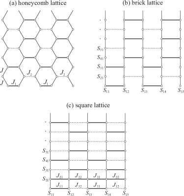
Figure 2: Lattices studied in the present paper. (a) The honeycomb lattice, (b) the brick lattice, and (c) the square lattice. (a) and (b) are equivalent. For the brick lattice (i.e., the honeycomb lattice), we assume that the interactions on the vertical bonds denoted by $J$ are uniform, while those on the horizontal bonds denoted by $J_{i}$ are uniform in a row but row-to-row random. As for the square lattice, we assume the same property of the interaction on the vertical bonds. The interactions on the horizontal bonds, however, are independently random in the adjoining two bonds and alternate in a row, and besides they are row-to-row random.

Let us begin with the honeycomb-lattice model. As shown in Fig. 2, the honeycomb lattice is equivalent to the brick lattice. We write the Ising spin sitting on each lattice point of the brick lattice as $S_{i,j}$, where $i$ and $j$ label vertical and horizontal positions respectively. We then assign a spin-spin interaction $J$ on the vertical bonds and $J_{i}$ on the horizontal bonds, where $i$ labels the vertical position of a bond. We assume that $J_{i}$’s are random and independent for different $i$. The Hamiltonian is written as

$$H = -J\sum_{i=1}^{M}\sum_{j=1}^{N}S_{i,j}S_{i+1,j}$$

$$-\sum_{\mu=1}^{M/2}\sum_{\nu=1}^{N/2}\left(J_{2\mu-1}S_{2\mu-1,2\nu-1}S_{2\mu-1,2\nu}+J_{2\mu}S_{2\mu,2\nu}S_{2\mu,2\nu+1}\right),$$

where $M$ and $N$ denote the number of sites on the vertical and horizontal lines respectively. We assume that $M$ and $N$ are even numbers. We consider two bimodal distributions for random $J_{i}$ as follows:

$$\begin{array}[]{l@{\hspace{1em}}l}\mbox{($\pm J$ model)}\hfil\hskip 10.00002pt&P(J_{i})=p\,\delta(J_{i}-J_{0})+(1-p)\,\delta(J_{i}+J_{0}),\\ \hfil\hskip 10.00002pt\\ \mbox{(diluted model)}\hfil\hskip 10.00002pt&P(J_{i})=p\,\delta(J_{i}-J_{0})+(1-p)\,\delta(J_{i}),\\ \end{array}$$ (2)

where $J_{0}>0$ and $0\leq p\leq 1$. Note that $p$ stands for the density of ferromagnetic bonds in the horizontal bonds. We moreover restrict ourselves to the range of $p$ such that $[J_{i}]>0$, where the notation $[\cdots]$ means the average over the randomness of the bonds:

$$[\cdots]=\int\prod_{i}dJ_{i}P(J_{i})(\cdots).$$ (3)

We next consider the square lattice. Same as the brick lattice, we assume that the interactions on the vertical bonds are uniform. Regarding the horizontal bonds, however, we assume that the interactions are random in the adjoining two bonds and form an alternating order, and besides they are independent in different rows. An instance of the configuration of interactions is depicted in Fig. 2(c). The Hamiltonian of the present model is given by

$$H = -J\sum_{i=1}^{M}\sum_{j=1}^{N}S_{i,j}S_{i+1,j}$$

$$-\sum_{i=1}^{M}\sum_{\nu=1}^{N/2}\left(J_{i1}S_{i,2\nu-1}S_{i,2\nu}+J_{i2}S_{i,2\nu}S_{i,2\nu+1}\right),$$

where $J_{i1}$ and $J_{i2}$ ($i=1,2,\cdots,M$) are independently random and follow Eq. (2).

For both lattices, we assume the periodic boundary condition in the horizontal direction ($S_{i,N+1}=S_{i,1}$) and in the vertical direction ($S_{M+1,j}=S_{1,j}$).

It should be noted that the $\pm J$ models on both lattices mentioned above are invariant under the change of the sign of all the horizontal couplings and that of the spins in every odd column. Therefore it turns out that the $\pm J$ models have the ferromagnetic-antiferromagnetic symmetry with respect to $p=1/2$.

3 Transfer matrices

We first focus on the square-lattice model. A portion of the Boltzmann factor regarding the lowest two layers in Fig. 2(c) is written as

$$\exp\left(\sum_{\nu=1}^{N/2}\left(K_{11}S_{1,2\nu-1}S_{1,2\nu}+K_{12}S_{1,2\nu}S_{1,2\nu+1}\right)+L\sum_{j=1}^{N}S_{1,j}S_{2,j}\right.$$

$$+\left.\sum_{\nu=1}^{N/2}\left(K_{21}S_{2,2\nu-1}S_{2,2\nu}+K_{22}S_{2,2\nu}S_{2,2\nu+1}\right)+L\sum_{j=1}^{N}S_{2,j}S_{3,j}\right),$$ (5)

where $K_{ij}=J_{ij}/T$ ($i=1,2,\cdots,M$; $j=1,2$) and $L=J/T$ with the temperature $T$ in the unit of $k_{B}=1$. The transfer matrix between the lowest and the second lowest rows is given by

$$T_{K_{11},K_{12},K_{21},K_{22}}(S_{11},\cdots,S_{1N};S_{31},\cdots,S_{3N})$$

$$=\sum_{S_{21},\cdots,S_{2N}}A_{K_{11},K_{12}}(S_{11},\cdots,S_{1N};S_{21},\cdots,S_{2N})$$

$$\hskip 56.9055pt\times A_{K_{21},K_{22}}(S_{21},\cdots,S_{2N};S_{31},\cdots,S_{3N}),$$ (6)

where

$$A_{K_{11},K_{12}}(S_{11},\cdots,S_{1N};S_{21},\cdots,S_{2N})$$

$$=\exp\left(\sum_{\nu=1}^{N/2}\left(K_{11}S_{1,2\nu-1}S_{1,2\nu}+K_{12}S_{1,2\nu}S_{1,2\nu+1}\right)+L\sum_{j=1}^{N}S_{1j}S_{2j}\right).$$ (7)

Using these $2^{N}\times 2^{N}$ transfer matrices, the partition function is written as

$$Z={\rm tr}\left(T_{K_{11},K_{12},K_{21},K_{22}}T_{K_{31},K_{32},K_{41},K_{42}}\cdots T_{K_{M-1,1},K_{M-1,2},K_{M1},K_{M2}}\right).$$ (8)

The matrices in Eqs. (7) are now written as

$$A_{K_{11},K_{12}}(S_{11},\cdots,S_{1N};S_{21},\cdots,S_{2N})=C\langle S_{11},\cdots,S_{1N}|\hat{A}_{K_{11},K_{12}}|S_{21},\cdots,S_{2N}\rangle$$ (9)

$$\hat{A}_{K_{11},K_{12}}=\exp\left(\sum_{\nu=1}^{N/2}\left(K_{11}\sigma_{2\nu-1}^{z}\sigma_{2\nu}^{z}+K_{12}\sigma_{2\nu}^{z}\sigma_{2\nu+1}^{z}\right)\right)\exp\left(g\sum_{j=1}^{N}\sigma_{j}^{x}\right)$$ (10)

where $\sigma_{j}^{\alpha}$ ($\alpha=x,y,z$) is the $\alpha$-component of the Pauli operator and $\{|S_{i1},\cdots,S_{iN}\rangle\}$ is the basis of an $N$-spin system satisfying $\sigma_{j}^{z}|S_{i1},\cdots,S_{iN}\rangle=S_{ij}|S_{i1},\cdots,S_{iN}\rangle$ for $j=1,2,\cdots,N$. $C$ and $g$ are defined by

$$C=\left(\frac{1}{2}\sinh 2g\right)^{-N/2},~{}~{}~{}g=\frac{1}{2}\log\coth L.$$ (11)

We introduce Majorana fermions and their Fourier transformations as follows;

$$\psi_{1}(\nu)=\frac{1}{\sqrt{2}}\left(\prod_{k=1}^{2\nu-2}\sigma_{k}^{x}\right)\sigma_{2\nu-1}^{z},\quad\psi_{2}(\nu)=\frac{1}{\sqrt{2}}\left(\prod_{k=1}^{2\nu-2}\sigma_{k}^{x}\right)\sigma_{2\nu-1}^{y},$$ (12)

$$\psi_{3}(\nu)=\frac{1}{\sqrt{2}}\left(\prod_{k=1}^{2\nu-1}\sigma_{k}^{x}\right)\sigma_{2\nu}^{z},\quad\psi_{4}(\nu)=\frac{1}{\sqrt{2}}\left(\prod_{k=1}^{2\nu-1}\sigma_{k}^{x}\right)\sigma_{2\nu}^{y},$$ (13)

$$\psi_{n}(\nu)=\sqrt{\frac{2}{N}}\sum_{0<q<\pi}\left(c_{n}(q)e^{iq\nu}+c_{n}^{\dagger}(q)e^{-iq\nu}\right),$$ (14)

where $n=1,2,3,4$ and $\nu$ runs from $1$ to $N/2$. Although the possible values of the wave number $q$ depend on the parity of $\prod_{j=1}^{N}\sigma_{j}^{x}$, they have no effect on the argument below and hence we do not care about them. Then $\hat{A}_{K_{11},K_{12}}$ in Eq. (9) is written as $\hat{A}_{K_{11},K_{12}}=\exp(H_{K_{11},K_{12}}^{(1)})\exp(H_{g}^{(2)})$, where

$$H_{K_{11},K_{12}}^{(1)} = 2i\sum_{\nu=1}^{N/2}\left(K_{11}\psi_{2}(\nu-1)\psi_{3}(\nu)+K_{12}\psi_{4}(\nu)\psi_{1}(\nu+1)\right)$$ (15)

$$= 2i\sum_{0<q<\pi}\left\{K_{11}\left(c_{2}(q)c_{3}^{\dagger}(q)+c_{2}^{\dagger}(q)c_{3}(q)\right)\right.$$

$$~{}~{}~{}~{}~{}~{}+\left.K_{12}\left(e^{-iq}c_{4}(q)c_{1}^{\dagger}(q)+e^{iq}c_{4}^{\dagger}(q)c_{1}(q)\right)\right\}$$

$$\equiv \sum_{0<q<\pi}h_{K_{11},K_{12}}^{(1)}(q),$$

$$H_{g}^{(2)} = 2ig\sum_{\nu=1}^{N/2}\left(\psi_{1}(\nu)\psi_{2}(\nu)+\psi_{3}(\nu)\psi_{4}(\nu)\right)$$ (16)

$$= 2ig\sum_{0<q<\pi}\left(c_{1}(q)c_{2}^{\dagger}(q)+c_{1}^{\dagger}(q)c_{2}(q)+c_{3}(q)c_{4}^{\dagger}(q)+c_{3}^{\dagger}(q)c_{4}(q)\right)$$

$$\equiv \sum_{0<q<\pi}h_{g}^{(2)}(q).$$

Since each mode is decoupled from others, the transfer matrices are given by a product of those with a fixed mode. Hence one gets

$$Z=\prod_{0<q<\pi}{\rm tr}\left\{\hat{\mathcal{A}}_{K_{11},K_{12}}(q)\hat{\mathcal{A}}_{K_{21},K_{22}}(q)\cdots\hat{\mathcal{A}}_{K_{M1},K_{M2}}(q)\right\},$$ (17)

where

$$\hat{\mathcal{A}}_{K_{11},K_{12}}(q)=\exp(h_{K_{11},K_{12}}^{(1)}(q))\exp(h_{g}^{(2)}(q)).$$ (18)

Taking the limit $N\to\infty$, the free energy per spin is written as

$$f=\int_{0}^{\pi}\frac{dq}{2\pi}f(q),$$ (19)

where

$$f(q)=-T\frac{1}{M}\ln{\rm tr}\left\{\hat{\mathcal{A}}_{K_{11},K_{12}}(q)\hat{\mathcal{A}}_{K_{21},K_{22}}(q)\cdots\hat{\mathcal{A}}_{K_{M1},K_{M2}}(q)\right\}.$$ (20)

In order to seek the critical temperature, we will investigate $f_{0}=\lim_{M\to\infty}f(0)$. We will see in fact that $f_{0}$ is non-analytic at a critical point $T_{\rm c}$.

In order to simplify $\hat{\mathcal{A}}_{K_{11},K_{12}}(0)$ further, we introduce new Majorana fermions as

$$c_{n}(q)=\frac{1}{\sqrt{2}}\left(\alpha_{n}(q)+i\beta_{n}(q)\right),\qquad c_{n}(q)^{\dagger}=\frac{1}{\sqrt{2}}\left(\alpha_{n}(q)-i\beta_{n}(q)\right).$$ (21)

The transfer matrices are rewritten in terms of these new Majorana fermions as

$$h_{K_{11},K_{12}}^{(1)}(q) = 2iK_{11}\left(\alpha_{2}\alpha_{3}+\beta_{2}\beta_{3}\right)$$ (22)

$$+2iK_{12}\left[\cos q\left(\alpha_{4}\alpha_{1}+\beta_{4}\beta_{1}\right)-\sin q\left(\alpha_{4}\beta_{1}+\alpha_{4}\beta_{1}\right)\right],$$

$$h_{g}^{(2)}(q) = 2ig\left(\alpha_{1}\alpha_{2}+\alpha_{3}\alpha_{4}+\beta_{1}\beta_{2}+\beta_{3}\beta_{4}\right),$$ (23)

where we have omitted $(q)$ on $\alpha_{n}$ and $\beta_{n}$. It is clear in the above that $\alpha_{n}$ and $\beta_{n}$ are completely decoupled and symmetric in the limit $q\rightarrow 0$. Hence the trace in Eq. (20) with $q\to 0$ is given by the square of the trace on the $\alpha$ subspace.

Now, focusing on $q\to 0$, we transform Majorana operators $\alpha_{n}$ into the Pauli matrices $\tau_{n}^{x}$, $\tau_{n}^{y}$ and $\tau_{n}^{z}$ as

$$\alpha_{1}=\frac{1}{\sqrt{2}}\tau_{1}^{z},\quad\alpha_{2}=\frac{1}{\sqrt{2}}\tau_{1}^{y},\quad\alpha_{3}=\frac{1}{\sqrt{2}}\tau_{1}^{x}\tau_{2}^{z},\quad\alpha_{4}=\frac{1}{\sqrt{2}}\tau_{1}^{x}\tau_{2}^{y}.$$ (24)

Then we obtain

$$2i(K_{11}\alpha_{2}\alpha_{3}+K_{12}\alpha_{4}\alpha_{1})=(K_{11}-K_{12}V)\tau_{1}^{z}\tau_{2}^{z},$$ (25)

$$2ig(\alpha_{1}\alpha_{2}+\alpha_{3}\alpha_{4})=g(1+V)\tau_{1}^{x},$$ (26)

where the unitary matrix $V$ is defined as $V=\tau_{1}^{x}\tau_{2}^{x}$. This matrix $V$ commutes with $h_{K_{11},K_{12}}^{(1)}(0)$ and $h_{g}^{(2)}(0)$ and has eigenvalues $\pm 1$. Thus the transfer matrix is decomposed into two on the subspaces with $V=\pm 1$ respectively. Therefore $f(0)$ in Eq. (20) is written as

$$f(0)=-2T\frac{1}{M}\ln\left({\rm tr}\prod_{i=1}^{M}A_{i}^{+}+{\rm tr}\prod_{i=1}^{M}A_{i}^{-}\right),$$ (27)

where $A_{i}^{+}$ and $A_{i}^{-}$ are $2\times 2$ matrices on the subspaces with $V=1$ and $V=-1$, respectively. We take the basis for the $V=1$ sector as eigenstates of $\tau_{1}^{z}\tau_{2}^{z}$, i.e.,

$$|+\rangle=\frac{1}{\sqrt{2}}\left(\left|\uparrow\uparrow\right\rangle+\left|\downarrow\downarrow\right\rangle\right),\qquad|-\rangle=\frac{1}{\sqrt{2}}\left(\left|\uparrow\downarrow\right\rangle+\left|\downarrow\uparrow\right\rangle\right).$$ (28)

Using this set of basis, $A_{i}^{+}$ is written in the matrix representation as

$$A_{i}^{+}=\left(\begin{array}[]{cc}e^{K_{i1}-K_{i2}}&0\\ 0&e^{-(K_{i1}-K_{i2})}\end{array}\right)\left(\begin{array}[]{cc}\cosh 2g&\sinh 2g\\ \sinh 2g&\cosh 2g\end{array}\right).$$ (29)

For the $V=-1$ sector, we settle the basis as

$$|+\rangle=\frac{1}{\sqrt{2}}\left(\left|\uparrow\uparrow\right\rangle-\left|\downarrow\downarrow\right\rangle\right),\qquad|-\rangle=\frac{1}{\sqrt{2}}\left(\left|\uparrow\downarrow\right\rangle-\left|\downarrow\uparrow\right\rangle\right).$$ (30)

Then one obtains the matrix representation of $A_{i}^{-}$,

$$A_{i}^{-}=\left(\begin{array}[]{cc}e^{K_{i1}+K_{i2}}&0\\ 0&e^{-(K_{i1}+K_{i2})}\end{array}\right).$$ (31)

The second term in the brackets of Eq. (27), i.e., the trace of a product of $A_{i}^{-}$ is estimated as $e^{2[K_{ij}]M}$ for large $M$, since it is the trace of the diagonal matrices. Regarding the first term, we define the Lyapunov exponent of a product of random matrices by

$$\gamma=\lim_{M\rightarrow\infty}\frac{1}{M}\ln{\rm tr}\prod_{i=1}^{M}A_{i}^{+}.$$ (32)

Using this, the first term is estimated as $e^{\gamma M}$. Therefore $f_{0}$ is obtained finally as

$$f_{0}=-2T\max\left\{\gamma,2[K_{ij}]\right\}.$$ (33)

The critical point is determined as a singular point of this quantity.

3.1 Honeycomb lattice

The model for the honeycomb lattice is obtained by making $(K_{i1},K_{i2})=(0,K_{i})$ for $i=2,4,\cdots,M$ and $(K_{i1},K_{i2})=(K_{i},0)$ for $i=1,3,\cdots,M-1$ in the above formulas on the square lattice with $K_{i}\equiv J_{i}/T$. Therefore one gets the following result instead of Eq. (33).

$$f_{0}=-2T\max\left\{\kappa,[K_{i}]\right\},$$ (34)

where

$$\kappa=\lim_{M\rightarrow\infty}\frac{1}{M}\ln{\rm tr}\prod_{\mu=1}^{M/2}B_{2\mu-1}^{+}B_{2\mu}^{-},$$ (35)

$$B_{i}^{\pm}=\left(\begin{array}[]{cc}e^{\pm K_{i}}&0\\ 0&e^{\mp K_{i}}\end{array}\right)\left(\begin{array}[]{cc}\cosh 2g&\sinh 2g\\ \sinh 2g&\cosh 2g\end{array}\right).$$ (36)

The relation between $B_{i}^{+}$ and $B_{i}^{-}$,

$$B_{i}^{-}=UB_{i}^{+}U,\qquad U\equiv\left(\begin{array}[]{cc}0&1\\ 1&0\end{array}\right),$$ (37)

yields a simpler representation of Eq. (35) as follows.

$$\kappa=\lim_{M\rightarrow\infty}\frac{1}{M}\ln{\rm tr}\prod_{i=1}^{M}B_{i},$$ (38)

where

$$B_{i}\equiv B_{i}^{+}U=\left(\begin{array}[]{cc}e^{K_{i}}&0\\ 0&e^{-K_{i}}\end{array}\right)\left(\begin{array}[]{cc}\sinh 2g&\cosh 2g\\ \cosh 2g&\sinh 2g\end{array}\right).$$ (39)

4 Pure systems

For the sake of confirmation, we visit the pure honeycomb-lattice model in the present section, before going to the random case. In the pure system, $K_{i}$ is no longer random and, supposing $K_{i}=K=J_{0}/T$ uniformly for any $i$, Eqs. (34), (38) and (39) reduce to

$$f_{0}=-2T\max\left\{\kappa,K\right\}$$ (40)

and

$$\kappa=\lim_{M\rightarrow\infty}\frac{1}{M}\ln{\rm tr}B^{M}=\ln\lambda,$$ (41)

$$B=\left(\begin{array}[]{cc}e^{K}&0\\ 0&e^{-K}\end{array}\right)\left(\begin{array}[]{cc}\sinh 2g&\cosh 2g\\ \cosh 2g&\sinh 2g\end{array}\right),$$ (42)

where $\lambda$ is the largest eigenvalues of $B$. After a straightforward computation, one finds

$$\lambda=\cosh K\sinh 2g+\sqrt{1+\cosh^{2}K\sinh^{2}2g}.$$ (43)

Now, a simple algebra shows that the equation $\kappa=K$ reduces to

$$\tanh K=\frac{1}{\sinh 2L}.$$ (44)

We define the temperature $T_{\rm c}$ as the solution of this equation. Since we have

$$f_{0}=\left\{\begin{array}[]{@{\,}ll}-2J_{0}&\mbox{for $T<T_{\rm c}$}\\ -2T\ln\lambda&\mbox{for $T>T_{\rm c}$}\end{array}\right.,$$ (45)

$T=T_{\rm c}$ provides a singular point of $f_{0}$ and hence $f$.

In the special case where $L=K$, namely $J=J_{0}$, Eq. (44) is further simplified into

$$\cosh 2K=2.$$ (46)

This is nothing but the critical point of the Ising model on the isotropic honeycomb lattice [27].

5 Random systems

The transition points are determined by the equation $\kappa=\left[K_{i}\right]$ for the honeycomb lattice and $\gamma=2\left[K_{ij}\right]$ for the square lattice. In order to analyze these equations, we point out that the random matrices $A_{i}^{+}$ in Eq. (29) and $B_{i}$ in Eq. (39) have the same form as the transfer matrix of the one-dimensional random-field Ising model. Therefore the Lyapunov exponent $\kappa$ and $\gamma$ can be evaluated using techniques for the free energy of the one-dimensional systems. In this section, we obtain the exact value of the transition probability in the zero temperature limit and numerically calculate the phase boundary in the finite temperature, assuming $J=J_{0}$.

5.1 Zero temperature

In the zero temperature limit, the Lyapunov exponents $\gamma$ and $\kappa$ are regarded as ground-state energies of one-dimensional random Ising models. In general, it is a difficult task to obtain the exact ground-state energy of a random system. However, the exact Lyapunov exponent in the case of $J=J_{0}$ can be obtained by the method proposed in Ref. [14]. First we focus on the honeycomb lattice with the $\pm J$ distribution.

We consider a one-dimensional Ising-spin system defined by the transfer matrices $B_{i}$ in Eq. (39). Supposing that $Z_{i}^{\pm}$ denote the partition functions of this system with sites $1,2,\cdots,i$ under the fixed boundary condition $S_{i}=\pm 1$ respectively, they obey the following recursion relation

$$\left(\begin{array}[]{c}Z_{i+1}^{+}\\ Z_{i+1}^{-}\end{array}\right)=B_{i}\left(\begin{array}[]{c}Z_{i}^{+}\\ Z_{i}^{-}\end{array}\right),$$ (47)

where we assume the initial condition $Z_{1}^{+}=Z_{1}^{-}=1$. The asymptotic behavior of $Z_{i}^{\pm}$ for $i\gg 1$ in the low-temperature limit $K\equiv J/T\gg 1$ should be written in the form of

$$\left(\begin{array}[]{c}Z_{i}^{+}\\ Z_{i}^{-}\end{array}\right)\sim\left(\begin{array}[]{c}z^{x_{i}+a_{i}}\\ z^{x_{i}}\end{array}\right),$$ (48)

where $z=e^{K}$ and $x_{i}$ and $a_{i}$ are random exponents to be investigated below. We here omitted prefactors, since they do not affect the propery of the exponent in the zero-temperature limit. The ground-state energy per spin of the one-dimensional system is expressed as

$$\lim_{T\rightarrow 0}\frac{\kappa}{K}=\lim_{M\rightarrow\infty}\frac{x_{M}+\max\{a_{M},0\}}{M}=\lim_{M\rightarrow\infty}\frac{1}{M}\sum_{i=1}^{M}(x_{i+1}-x_{i}),$$ (49)

where we use the fact that the exponent $a_{M}$ does not diverge with $M$ as will be shown later. The last expression implies that the average increment of exponent $x_{i}$ corresponds to the Lyapunov exponent.

When $J_{i}=+J$, the random matrix $B_{i}$ has the asymptotic form

$$B_{i}=\left(\begin{array}[]{cc}z^{-1}&z\\ z^{-1}&z^{-3}\end{array}\right),$$ (50)

where we have used in Eq. (39)

$$\sinh 2g\sim z^{-2},\qquad\cosh 2g\sim 1.$$ (51)

Then the recursion relation of Eq. (47) with Eq. (48) is reduced to

$$x_{i+1} = x_{i}-1+\max\{a_{i},-2\}$$ (52)

$$a_{i+1} = \max\{a_{i},2\}-\max\{a_{i},-2\}.$$ (53)

Similarly, when $J_{i}=-J$, we obtain

$$x_{i+1} = x_{i}+1+\max\{a_{i},-2\}$$ (54)

$$a_{i+1} = \max\{a_{i},2\}-\max\{a_{i},-2\}-4.$$ (55)

Now, noting $a_{1}=0$, one can see that possible values of $a_{i}$ are restricted only to $0$, $\pm 2$, and $\pm 4$. The transition matrix which transforms $a_{i}$ to $a_{i+1}$ is given by

$$\bordermatrix{&a_{i}=4&a_{i}=2&a_{i}=0&a_{i}=-2&a_{i}=-4\cr a_{i+1}=4&0&0&0&p&p\cr a_{i+1}=2&0&0&p&0&0\cr a_{i+1}=0&p&p&0&\bar{p}&\bar{p}\cr a_{i+1}=-2&0&0&\bar{p}&0&0\cr a_{i+1}=-4&\bar{p}&\bar{p}&0&0&0\cr},$$ (56)

where $\bar{p}=1-p$. Since the Markov chain generated by this transition matrix is clearly irreducible and aperiodic except for non-random cases, it is ergotic and has the unique stationary distribution corresponding to the maximum eigenvalue of one. The distribution of $a_{i}$ converges in the limit $i\rightarrow\infty$ to this stationary distribution which is explicitly given by

$$P_{a}({+4})=\frac{p\bar{p}}{1+\bar{p}},\quad P_{a}({+2})=\frac{p(1-p\bar{p})}{(1+p)(1+\bar{p})},$$

$$P_{a}(0)=\frac{1-p\bar{p}}{(1+p)(1+\bar{p})},$$

$$P_{a}({-2})=\frac{\bar{p}(1-p\bar{p})}{(1+p)(1+\bar{p})},\quad P_{a}({-4})=\frac{p\bar{p}}{1+p}.$$

The increment of the exponent $x_{i}$ depends on $J_{i}$ and $\max\{a_{i},-2\}$ as shown Eqs. (52) and (54). Therefore, its average increment is computed by

$$(-p+\bar{p})+\left\{4P_{a}(+4)+2P_{a}(+2)-2P_{a}(-2)-2P_{a}(-4)\right\},$$ (57)

which yields the exact Lyapunov exponent in the zero-temperature limit

$$\lim_{T\rightarrow 0}\frac{\kappa}{K}=\frac{3p(1-p)}{(1+p)(2-p)}.$$ (58)

Finally, noting $[K_{i}]=(2p-1)K$ for the $\pm J$ model, we obtain the exact critical probability $p_{c}$ in the zero-temperature limit as

$$p_{\rm c}=1-2\sin\frac{\pi}{18}=0.65270364\cdots.$$ (59)

A similar calculation for the square lattice yields

$$\lim_{T\rightarrow 0}\frac{\gamma}{K}=2p(1-p),$$ (60)

and the critical probability

$$p_{\rm c}=\frac{\sqrt{5}-1}{2}=0.61803399\cdots,$$ (61)

which is equal to the inverse of the golden ratio.

In the diluted models, the Lyapunov exponents are obtained as

$$\lim_{T\rightarrow 0}\frac{\kappa}{K}=\frac{p(1-p)}{3-p},\qquad\lim_{T\rightarrow 0}\frac{\gamma}{K}=\frac{2p(1-p)}{3}.$$ (62)

The critical probability in the zero-temperature limit is $p_{\rm c}=0$ both for the honeycomb and square lattices. This result as well as the known fact that the pure system ($p=1$) has the ferromagnetic ground state lead to the conclusion that the zero-temperature phase of the diluted model for $p>0$ is ferromagnetic. This conclusion is naturally understood since this model is always percolated except $p=0$.

5.2 Finite temperatures

So far some methods have been developed to numerically compute the Lyapunov exponent of a product of random matrices. Mainieri proposed the cycle expansion method whose convergence is exponentially fast in the cycle length [19]. Bai improved this method using the evolution operator approach [2]. We emply this improved cycle expansion (ICE) method and the Monte Carlo method. The ICE method is summarized briefly in Appendix. Although we still consider $J=J_{0}$ for comparison with the zero-temperature results, numerical methods used in this section can be applied to $J\neq J_{0}$.

Figure 3: $p$ dependence of the Lyapunov exponent for the $\pm J$ model on the honeycomb lattice. The dashed line indicates $[K_{i}]/K$. The critical point corresponds to an intersection point between the curve of the Lyapunov exponent and the dashed line.

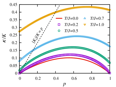
Figure 4: $p$ dependence of the Lyapunov exponent for the diluted model on the honeycomb lattice.

For the honeycomb-lattice model with $T/J\geq 0.7$, we used the ICE with the cycle length $n=20$, which produces more than $15$ reliable digits. For lower temperatures, however, the ICE needs a still longer cycle length to attain the convergence. This cost was complemented with the Monte Carlo method for $T/J<0.7$, where Lyapunov exponents were obtained by averaging over $1000$ configurations of a product of $10^{5}$ matrices with the standard error of $\kappa/K$ less than $6.0\times 10^{-5}$.

As for the square lattice, since the random matrix $A_{i}^{+}$ has three possible choices, the ICE needs more computational cost as well as longer cycle length for convergence than the honeycomb lattice. Therefore we used the ICE with the cycle length $n=15$ for $T/J\geq 1.0$ and the Monte Carlo method for $T/J<1.0$. Results by ICE have the same accuracy as the honeycomb lattice, while the standard errors of $\gamma/K$ by the Monte Carlo method are less than $9.0\times 10^{-5}$.

The $p$ dependence of the Lyapunov exponent for the $\pm J$ model on the honeycomb lattice is shown in Fig. 3. The solid curve indicates the exact result (58) in the zero-temperature limit. The critical points are determined by the intersection point with the dashed line ($[K_{i}]/K=2p-1$). The zero-temperature critical point is given exactly by Eq. (59). In Fig. 4 we show the results for the diluted model. It is clear that the critical probability in the zero-temperature limit is equal to zero as mentioned before.

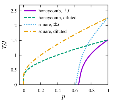
Figure 5: Critical lines in the $p-T$ plane of the $\pm J$ models and the diluted models on the honeycomb and squara lattices.

The critical line in the $p-T$ plane were obtained by solving the equation $\kappa=[K_{i}]$ or $\gamma=2[K_{ij}]$. For the temperature region where the ICE is valid, we estimated the critical temperature using the bisection method for given $p$’s. On the other hand, for lower temperatures, we obtained the critical probability for given $T$’s using the Monte Carlo method and the bisection method. The results are shown in Fig. 5. Although one cannot say anything about the property of the phases away from the critical line, it has been shown exactly that the critical temperature at $p=1$ is the transition point between the high-temperature paramagnetic phase and the low-temperature ferromagnetic phase. This fact as well as the fact that the critical line obtained here is continuously connected with the $p=1$ transition point imply that the critical line is in fact the transition line separating the paramagnetic and ferromagnetic phases. It is worth noting that the $\pm J$ model has the ferromagntic-antiferromagnetic symmetry with respect to $p=1/2$, as mentioned in Sect. 2. Therefore, we deduce that there is a striped antiferromagnetic phase in the small $p$ region, though it is not shown in Fig. 5. In addition, the study on the Shanker-Murthy model suggests that the Griffiths phase may exist between the ferromagnetic and antiferromagnetic phases and below the critical temperature of the pure system [8, 22].

We comment that Hoever [10] has numerically studied the critical line of the $\pm J$ model on the square lattice. Our result on the same model is in perfect agreement with it.

It should be pointed that the critical lines of the $\pm J$ model on both lattices are not vertical near zero temperature on the $p-T$ plane. As shown in Fig. 6, the Lyapunov exponent $\kappa$ devided by $K$ at low temperature seems to have a form

$$\kappa/K\simeq e_{0}(p)+cT,$$ (63)

where $e_{0}(p)$ denotes the zero-temperature limit of $\kappa/K$ which is exactly given by Eq. (58). The coefficient $c$ is estimated as $c=0.1509$ by fitting the data at $p=p_{c}$ for $0\leq T/J<0.2$. This observation implies that the critical temperature for $T/J\ll 1$ is behaves as

$$T_{c}(p)\simeq\frac{1}{c}\left\{(2p-1)-e_{0}(p)\right\}\simeq 15.70\times(p-p_{c}),$$ (64)

which is consistent with our numerical result (Fig. 5). On the square lattice, we obtain $T_{c}(p)\simeq 14.64\times(p-p_{c})$.

These behaviors of the critical temperature are quite different from the Shankar-Murthy model, where the constraint $K_{i1}=K_{i2}$ leads to the exact Lyapunov exponent $\gamma=2g$ regardless of $p$. Then an essential singularity of $g\sim e^{-2J/T}$ at $T=0$ causes the vertical growth of the critical temperature at $p_{c}=1/2$.

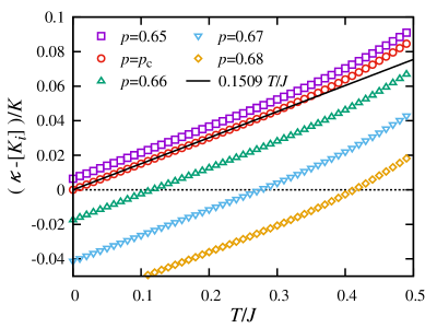
Figure 6: Low-temperature behavior of the Lyapunov exponent for the $\pm J$ model on the honeycomb lattice. The solid line is obtained by fitting the data at $p=p_{c}$ for $0\leq T/J<0.2$. The intersection with the horizontal dashed line indicates the transition temperature.

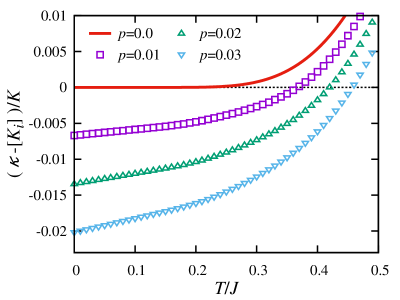
Figure 7: Low-temperature behavior of the Lyapunov exponent for the diluted model on the honeycomb lattice.

In contrast to the $\pm J$ models, the diluted model has the vertical phase boundary in the same way as the Shankar-Murthy model. The Lyapunov exponent at $p=0$ is exactly calculated as $\kappa=2g$ for the honeycomb lattice, which is essentially singular with respect to $T$. The low-temperature behavior of the Lyapunov exponent is shown in Fig. 7.

6 Conclusion

In this paper, we discussed the two-dimensional Ising model with striped randomness on the honeycomb lattice and on the square lattice. We simplified the transfer matrices by using the Majorana fermion operators and obtained the $2\times 2$ matrix representation in the long-wavelength limit. The Lyapunov exponents can be calculated by regarding these decomposed matrices as the transfer matrix of the one-dimensional random-field Ising model. We obtained its exact solution in the zero-temperature limit and determined the exact value for the critical probability $p_{c}$ of ferromagnetic bonds. The critical line on the probability-temperature ($p-T$) plane was also calculated with highly accurate numerical methods.

We focus only on the zero wave-number limit to analyze the critical point. However the wave-number dependence of the free energy is necessary to analyze critical phenomena and to determine the universality class, which remains as one of the future issues.

Appendix A Cycle expansion of the Lyapunov exponent

In this appendix, we briefly summarize the improved cycle expansion method as a numerical method to compute the Lyapunov exponent.

The Lyapunov exponent of a product of random matrices is defined as

$$\gamma=\lim_{n\rightarrow\infty}\frac{1}{n}\left\langle\ln\left\|M_{1}M_{2}\cdots M_{n}\right\|\right\rangle$$ (65)

where $M_{i}$ is a random matrix and the angular brackets denote the ensemble average. It is notable that the Lyapunov exponent is independent of a choice of the matrix norm $\|\cdot\|$ as long as equivalent norm used. The maximum eigenvalue $\mu_{0}(M)$ is the most convenient norm to derive the cycle expansion because it is invariant under cyclic rotation $\mu_{0}(M_{i}M_{j})=\mu_{0}(M_{j}M_{i})$ and satisfies $\mu_{0}(M^{2})=\mu_{0}(M)^{2}$.

Assume that the random matrix $M_{i}$ has $m$ possible choices to be $M_{i}=A_{s}$ with probability $p_{s}$ $(s=1,2,\cdots,m)$. With a string of $n$ choices $S\equiv s_{1}s_{2}\cdots s_{n}$, the product of $n$ random matrices $A_{s_{1}}A_{s_{2}}\cdots A_{s_{n}}$ is denoted by $A_{S}$ and its probability is by $P(S)\equiv\prod_{i=1}^{n}p_{s_{i}}$. With these notations, the Lyapunov exponent is expressed as the large-$n$ limit of the following quantity

$$\gamma_{n}\equiv\frac{1}{n}\sum_{|S|=n}P(S)\ln\mu_{0}(A_{S}),$$ (66)

where $|S|$ is the length of a string $S$.

Owing to the properties of $\mu_{0}(A)$, the sum in Eq. (66) is decomposed into the sum over the set $C_{p}$ of all possible primitive cycles, where a cycle is said primitive if it is not a repeat of a smaller length cycle. Two cycles are equivalent if they differ only by a cyclic rotation. For example, $s_{1}s_{2}s_{1}s_{2}\not\in C_{p}$ because it is a repeat of $s_{1}s_{2}$, and if $s_{1}s_{2}s_{3}\in C_{p}$, $s_{2}s_{3}s_{1}\not\in C_{p}$. As a result, the cycle expansion of the Lyapunov exponent is obtained as

$$\gamma_{n}=\sum_{S\in C_{p}}\sum_{r=1}^{n}\delta_{r|S|,n}P(S)^{r}\ln\mu_{0}(A_{S}).$$ (67)

This formula was also derived from the expansion of the thermodynamic zeta function and its exponential convergence with the cycle length was observed [19].

Bai proposed an accelerated algorithm for the cycle expansion based on the evolution operator approach [2]. Bai numerically showed super-exponential convergence of the weighted average of the cycle expansion,

$$\tilde{\gamma}_{n}=\frac{\sum_{k=0}^{n-1}w_{k}\gamma_{n-k}}{\sum_{k=0}^{n-1}w_{k}},$$ (68)

in contrast to exponential convergence of the cycle expansion method. The averaging weight $w_{k}$ is determined to eliminate all exponential converging terms by using the evolution operator approach. In the case of $2\times 2$ matrices with positive elements, $w_{k}$ is given by

$$w_{k}=-\frac{1}{k}\sum_{j=1}^{k}c_{j}w_{k-j},$$ (69)

$$c_{n}=\sum_{S\in C_{p}}\sum_{r=1}^{n}\delta_{r|S|,n}|S|\frac{\left[P(S)g(A_{S})\right]^{r}}{1-g(A_{S})^{r}},$$ (70)

where $g(A)$ denotes the ratio of the second eigenvalue of $A$ to the first one $\mu_{0}(A)$.

acknowledgements

SM would like to thank T. Hamasaki and H. Nishimori for helpful advices. The work of SS was supported by the JSPS (grant No. 26400402).

References

- [1] Aharony, A., Stephen, M.J.: Duality relations and the replica method for Ising models. J. Phys. C: Solid State Phys. 13, L407–L414 (1980)
- [2] Bai, Z.Q.: On the cycle expansion for the Lyapunov exponent of a product of random matrices. J. Phys. A: Math. Theor. 40, 8315–8328 (2007)
- [3] Chaloupka, J., Jackeli, G., Khaliullin, G.: Kitaev-Heisenberg model on a honeycomb lattice: Possible exotic phases in iridium oxides . Phys. Rev. Lett. 105, 027204 (2010)
- [4] Chaloupka, J., Jackeli, G., Khaliullin, G.: Zigzag magnetic order in the iridium oxide . Phys. Rev. Lett. 110, 097204 (2013)
- [5] Choi, S.K., Coldea, R., Kolmogorov, A.N., Lancaster, T., Mazin, I.I., Blundell, S.J., Radaelli, P.G., Singh, Y., Gegenwart, P., Choi, K.R., Cheong, S.W., Baker, P.J., Stock, C., Taylor, J.: Spin waves and revised crystal structure of honeycomb iridate . Phys. Rev. Lett. 108, 127204 (2012)
- [6] Domany, E.: Criticality and crossover in the bond-diluted random Ising model. J. Phys. C: Solid State Phys. 11, L337–L342 (1978)
- [7] Fisch, R.: Critical temperature for two-dimensional Ising ferromagnets with quenched bond disorder. J. Stat. Phys. 18, 111–114 (1978)
- [8] Griffiths, R.B.: Nonanalytic behavior above the critical point in a random Ising ferromagnet. Phys. Rev. Lett. 23, 17–19 (1969)
- [9] Hamm, J.R.: Regularly spaced blocks of impurities in the Ising model: Critical temperature and specific heat. Phys. Rev. B 15, 5391–5411 (1977)
- [10] Hoever, P.: Generalized transfer formalism and application to random Ising models. Z. Phys. B Condensed Matter 48, 137–148 (1982)
- [11] Houtappel, R.: Order-disorder in hexagonal lattices. Physica 16, 425–455 (1950)
- [12] Iglói, F., Lajkó, P.: On the critical temperature of non-periodic Ising models on hexagonal lattices. Z. Phys. B Condensed Matter 99, 281–283 (1995)
- [13] Jackeli, G., Khaliullin, G.: Mott insulators in the strong spin-orbit coupling limit: From Heisenberg to a quantum compass and Kitaev models. Phys. Rev. Lett. 102, 017205 (2009)
- [14] Kadowaki, T., Nonomura, Y., Nishimori, H.: Exact ground-state energy of the Ising spin glass on strips. J. Phys. Soc. Jpn. 65, 1609–1616 (1996)
- [15] Kardar, M., Berker, A.N.: Exact criticality condition for randomly layered Ising models with competing interactions on a square lattice. Phys. Rev. B 26, 219–225 (1982)
- [16] Kaufman, B.: Crystal statistics. II. Partition function evaluated by spinor analysis. Phys. Rev. 76, 1232–1243 (1949)
- [17] Kitaev, A.: Anyons in an exactly solved model and beyond. Ann. Phys. 321, 2–111 (2006)
- [18] Kramers, H.A., Wannier, G.H.: Statistics of the two-dimensional ferromagnet. Part I. Phys. Rev. 60, 252–262 (1941)
- [19] Mainieri, R.: Zeta function for the Lyapunov exponent of a product of random matrices. Phys. Rev. Lett. 68, 1965–1968 (1992)
- [20] McCoy, B.M., Wu, T.T.: Theory of a two-dimensional Ising model with random impurities. I. Thermodynamics. Phys. Rev. 176, 631–643 (1968)
- [21] Onsager, L.: Crystal statistics. I. A two-dimensional model with an order-disorder transition. Phys. Rev. 65, 117–149 (1944)
- [22] Randeria, M., Sethna, J.P., Palmer, R.G.: Low-frequency relaxation in Ising spin-glasses. Phys. Rev. Lett. 54, 1321–1324 (1985)
- [23] Reuther, J., Thomale, R., Trebst, S.: Finite-temperature phase diagram of the Heisenberg-Kitaev model. Phys. Rev. B 84, 100406 (2011)
- [24] Schwartz, M.: Dual relations for quenched random systems. Phys. Lett. A 75, 102–104 (1979)
- [25] Shankar, R., Murthy, G.: Nearest-neighbor frustrated random-bond model in : Some exact results. Phys. Rev. B 36, 536–545 (1987)
- [26] Singh, Y., Manni, S., Reuther, J., Berlijn, T., Thomale, R., Ku, W., Trebst, S., Gegenwart, P.: Relevance of the Heisenberg-Kitaev model for the honeycomb lattice iridates . Phys. Rev. Lett. 108, 127203 (2012)
- [27] Wannier, G.H.: The statistical problem in cooperative phenomena. Rev. Mod. Phys. 17, 50–60 (1945)
- [28] Wannier, G.H.: Antiferromagnetism. The triangular Ising net. Phys. Rev. 79, 357–364 (1950)
- [29] Wolff, W.F., Hoever, P., Zittartz, J.: Layered inhomogeneous Ising models with frustration on a square lattice. Z. Phys. B Condensed Matter 42, 259–264 (1981)
- [30] Ye, F., Chi, S., Cao, H., Chakoumakos, B.C., Fernandez-Baca, J.A., Custelcean, R., Qi, T.F., Korneta, O.B., Cao, G.: Direct evidence of a zigzag spin-chain structure in the honeycomb lattice: A neutron and X-ray diffraction investigation of single-crystal . Phys. Rev. B 85, 180403 (2012)