Quantifying the non-ergodicity of scaled Brownian motion

Abstract

We examine the non-ergodic properties of scaled Brownian motion, a non-stationary stochastic process with a time dependent diffusivity of the form $D(t)\simeq t^{\alpha-1}$. We compute the ergodicity breaking parameter EB in the entire range of scaling exponents $\alpha$, both analytically and via extensive computer simulations of the stochastic Langevin equation. We demonstrate that in the limit of long trajectory lengths $T$ and short lag times $\Delta$ the EB parameter as function of the scaling exponent $\alpha$ has no divergence at $\alpha=1/2$ and present the asymptotes for EB in different limits. We generalise the analytical and simulations results for the time averaged and ergodic properties of scaled Brownian motion in the presence of ageing, that is, when the observation of the system starts only a finite time span after its initiation. The approach developed here for the calculation of the higher time averaged moments of the particle displacement can be applied to derive the ergodic properties of other stochastic processes such as fractional Brownian motion.

1 Introduction

The non-Brownian scaling of the mean squared displacement (MSD) of a diffusing particle of the power-law form [1, 2, 3, 4]

$$\langle x^{2}(t)\rangle=2K_{\alpha}t^{\alpha}$$ (1)

is a hallmark of a wide range of anomalous diffusion processes [2, 4]. Equation (1) features the anomalous diffusion coefficient $K_{\alpha}$ of physical dimension $\mathrm{cm}^{2}/\mathrm{sec}^{\alpha}$ and the anomalous diffusion exponent $\alpha$. Depending on its magnitude we distinguish subdiffusion ($0<\alpha<1$) and superdiffusion ($\alpha>1$). Interest in anomalous diffusion processes was rekindled with the advance of modern spectroscopic methods, in particular, advanced single particle tracking methods [5]. Thus, subdiffusion was observed for the motion of biopolymers and submicron tracer particles in living biological cells [6], in complex fluids [7], as well as in extensive computer simulations of membranes [8] or structured systems [9], among others [3, 4, 10]. Superdiffusion of tracer particles was observed in living cells due to active motion [11].

Anomalous diffusion processes characterised by the MSD (1) may originate from a variety of distinct physical mechanisms [1, 3, 4, 10, 12, 13]. These include a power-law statistic of trapping times in the continuous time random walks (CTRWs) as well as related random energy models [4, 10, 12, 13, 14, 15] and CTRW variants with correlated jumps [16] or superimposed environmental noise [17]. Other models include random processes driven by Gaussian yet power-law correlated noise such as fractional Brownian motion (FBM) [18] or the fractional Langevin equation [19]. Closely related to these models is the subdiffusive motion on fractals such as critical percolation clusters [20]. Finally, among the popular anomalous diffusion models we mention heterogeneous diffusion processes with given space dependencies of the diffusion coefficient [21] as well as processes with explicitly time dependence diffusion coefficients, in particular, the scaled Brownian motion (SBM) with power-law form $D(t)\simeq t^{\alpha-1}$ analysed in more detail herein [22, 23, 24, 25]. Also combinations of space and time dependent diffusivities were investigated [23, 26]. Space and/or time dependent diffusivities were used to model experimental results for smaller tracer proteins in living cells [27] and anomalous diffusion in biological tissues [28] including brain matter [29, 30]. In particular, SBM was used to describe fluorescence recovery after photobleaching in various settings [31] as well as anomalous diffusion in various biophysical contexts [32]. In other branches of physics SBM was used to model turbulent flows observed by Richardson [33] as early as 1952 by Batchelor [34]. Moreover, the diffusion of particles in granular gases with relative speed dependent restitution coefficients follow SBM [35]. We note that in the limiting case $D(t)\sim 1/t$ the resulting process is ultraslow with a logarithmic growth of the MSD [36] known from processes such as Sinai diffusion [38], single file motion in ageing environments [39], or granular gas diffusion with constant restitution coefficient [36].

In the following we study the ergodic properties of SBM in the Boltzmann-Khinchin sense [37], finding that even long time averages of physical observables such as the MSD do not converge to the corresponding ensemble average [4, 12, 13, 40]. In particular we compute the ergodicity breaking parameter EB—characterising the trajectory-to-trajectory fluctuations of the time averaged MSD—in the entire range of the scaling exponents $\alpha$, both analytically and from extensive computer simulations. We generalise the results for the ergodic properties of SBM in the presence of ageing, when we start to evaluate the time average the MSD a finite time span after the initiation of the system.

The paper is organised as follows. In section 2 we summarise the observables computed and provide a brief overview of the basic properties of SBM. In section 3 we describe the theoretical concepts and numerical scheme employed in the paper. We present the main results for the EB parameter of non-ageing and ageing SBM in detail in sections 3 and 4. In section 5 we summarise our findings and discuss their possible applications and generalisations.

2 Observables and fundamental properties of scaled Brownian motion

We define SBM in terms of the stochastic process [4, 22, 24, 26, 43]

$$\frac{dx(t)}{dt}=\sqrt{2D(t)}\times\zeta(t),$$ (2)

where $\zeta(t)$ is white Gaussian noise with zero mean and unit amplitude $\langle\zeta(t_{1})\zeta(t_{2})\rangle=\delta(t_{1}-t_{2})$. The time dependent diffusion coefficient is taken as

$$D(t)=\alpha K_{\alpha}t^{\alpha-1},$$ (3)

where we require the positivity of the scaling exponent, $\alpha>0$. SBM is inherently out of thermal equilibrium in confining external potentials [25]. Let us briefly outline the basic properties of the SBM process. The ensemble averaged MSD of SBM scales anomalously with time in the form of equation (1).

Here and below we use the standard definition of the time averaged MSD [4, 12]

$$\overline{\delta^{2}(\Delta)}=\frac{1}{T-\Delta}\int\limits_{0}^{T-\Delta}\Big{[}x(t+\Delta)-x(t)\Big{]}^{2}dt,$$ (4)

where $\Delta$ is the lag time, or the width of the window slid along the time series in taking the time average (4). Moreover, $T$ is the total length of the time series. We denote ensemble averages by the angular brackets while time averages are indicated by the overline. Often, an additional average of the form

$$\left<\overline{\delta^{2}(\Delta)}\right>=\frac{1}{N}\sum_{i=1}^{N}\overline{\delta^{2}_{i}(\Delta)}$$ (5)

is performed over $N$ realisations of the process, to obtain smoother curves. From a mathematical point of view, this trajectory average allows the calculation of the time averaged MSD for processes, which are not self-averaging [4, 40] Both quantities (4) and (5) are important in the analysis of single particle trajectories measured in advanced tracking experiments [12]. For SBM the mean time averaged MSD (5) grows as [25]

$$\left<\overline{\delta^{2}(\Delta)}\right>=\frac{2K_{\alpha}\left[T^{\alpha+1}-\Delta^{\alpha+1}-(T-\Delta)^{\alpha+1}\right]}{(\alpha+1)(T-\Delta)}.$$ (6)

In the limit $\Delta/T\ll 1$, the time averaged MSD scales linearly with the lag time,

$$\left<\overline{\delta^{2}(\Delta)}\right>\sim 2K_{\alpha}\frac{\Delta}{T^{1-\alpha}}.$$ (7)

SBM is thus a weakly non-ergodic process in Bouchaud’s sense [44]: the ensemble and time averaged MSDs are disparate even in the limit of long observation times $T$, $\lim_{T\to\infty}\overline{\delta^{2}(\Delta)}\neq\langle x^{2}(t)\rangle$ and thus violate the Boltzmann-Khinchin ergodic hypothesis, while the entire phase space is accessible to any single particle. Moreover, the magnitude of the time averaged MSD becomes a function of the trace length $T$. Analogous asymptotic forms for the mean time averaged MSD (5) are found in subdiffusive CTRW processes [40, 41] and heterogeneous diffusion processes [21], see also the extensive recent review [4]. Note that also much weaker forms of non-ergodic behaviour exist for Lévy processes [42].

Another distinct feature of weakly non-ergodic processes of the subdiffusive CTRW [40] and heterogeneous diffusion type [21] is the fact that time averaged observables remain random quantities even in the long time limit and thus exhibit a distinct scatter of amplitudes between individual realisations for a given lag time. This irreproducibility due to the scatter of individual traces $\overline{\delta^{2}(\Delta)}$ around their mean is described by the ergodicity breaking parameter [4, 40, 45, 46]

$$\mathrm{EB}(\Delta)=\frac{\left<\left(\overline{\delta^{2}(\Delta)}\right)^{2}\right>-\left<\overline{\delta^{2}(\Delta)}\right>^{2}}{\left<\overline{\delta^{2}(\Delta)}\right>^{2}}=\frac{\mathcal{N}(\Delta)}{\mathcal{D}(\Delta)}=\left<\xi^{2}(\Delta)\right>-1,$$ (8)

where $\xi(\Delta)=\overline{\delta^{2}(\Delta)}\Big{/}\left<\overline{\delta^{2}(\Delta)}\right>$. Moreover, we introduced the abbreviations $\mathcal{N}(\Delta)$ and $\mathcal{D}(\Delta)$ for the nominator and denominator of EB, respectively. This notation will be used below. For Brownian motion in the limit $\Delta/T\to 0$ the EB parameter vanishes linearly with $\Delta/T$ in the form [4, 45]

$$\mathrm{EB}_{\mathrm{BM}}(\Delta)=\frac{4\Delta}{3T}.$$ (9)

In contrast to subdiffusive CTRW and heterogeneous diffusion processes, the EB parameter of SBM vanishes in the limit $\Delta/T\to 0$ and in this sense the time averaged observable becomes reproducible [24, 25, 43]. We demonstrate the small amplitude scatter of SBM in figure 1, for a detailed discussion see below. We note that the scatter of the time averaged MSD of SBM around the ergodic value $\xi=1$ becomes progressively asymmetric for smaller $\alpha$ values and in later parts of the time averaged trajectories, see Fig. 6 of reference [4]. In the following we derive the exact analytical results for the EB parameter of SBM and support these results with extensive computer simulations. Moreover we extend the analytical and computational analysis of the EB parameter to the case of the ageing SBM process when we start evaluating the time series $x(t)$ at the time $t_{a}>0$ after the original initiation of the system at $t=0$ [43].

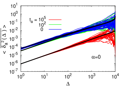
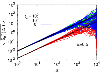
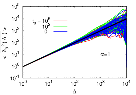
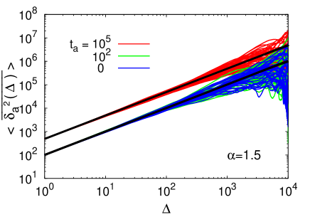
Figure 1: Time averaged MSD of SBM as function of the lag time $\Delta$ for several values of the scaling exponents $\alpha$ and ageing times $t_{a}$. The asymptotic behaviour of equation (11) is shown by the black solid lines. Parameters: $T=10^{4}$, $t_{a}=0$, $10^{2}$, $10^{5}$, and $N=100$ traces are shown.

The time averaged MSD of an ageing stochastic process is defined as [15]

$$\overline{\delta^{2}_{a}(\Delta)}=\frac{1}{T-\Delta}\int_{t_{a}}^{t_{a}+T-\Delta}\Big{[}x(t+\Delta)-x(t)\Big{]}^{2}dt$$ (10)

and thus again involves the observation time $T$. The properties ageing SBM were considered recently [43]. The mean time averaged MSD becomes

$$\left<\overline{\delta^{2}_{a}(\Delta)}\right> = \frac{2K_{\alpha}}{(\alpha+1)(T-\Delta)}\Big{[}(T+t_{a})^{\alpha+1}-(t_{a}+\Delta)^{\alpha+1}$$ (11)

$$-(T+t_{a}-\Delta)^{\alpha+1}+t_{a}^{\alpha+1}\Bigg{]}.$$

The ratio of the aged versus the non-ageing time averaged MSD in the limit $\Delta\ll t_{a},T$ has the asymptotic form [43]

$$\Lambda_{\alpha}(t_{a}/T)=\frac{\left<\overline{\delta^{2}_{a}(\Delta)}\right>}{\left<\overline{\delta^{2}(\Delta)}\right>}\sim(1+t_{a}/T)^{\alpha}-(t_{a}/T)^{\alpha}.$$ (12)

This functional form is identical to that obtained for subdiffusive CTRWs [15] and heterogeneous diffusion processes [47]. The factor $\Lambda_{\alpha}(z)$ quantifies the respective depression and enhancement of the time averaged MSD for the cases of ageing sub- and superdiffusive SBM.

Figure 1 shows the time averaged MSD $\overline{\delta^{2}(\Delta)}$ of individual SBM traces for the case of weak, intermediate, and strong ageing for different values of $\alpha$. We observe that the spread of individual $\overline{\delta^{2}(\Delta)}$ changes only marginally with progressive ageing times $t_{a}$. Also the changes with the scaling exponent $\alpha$ are modest, compare figure 2. Also note that the magnitude of the time averaged MSD decreases with $t_{a}$ for ultraslow SBM at $\alpha=0$, stays independent on $t_{a}$ for Brownian motion at $\alpha=1$, and increases with the ageing time for superdiffusive processes at $\alpha>1$. These trends are in agreement with the theoretical predictions of equation (11) shown as the solid lines in figure 1.

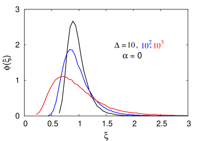
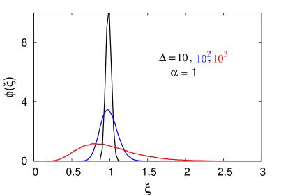
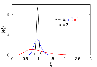
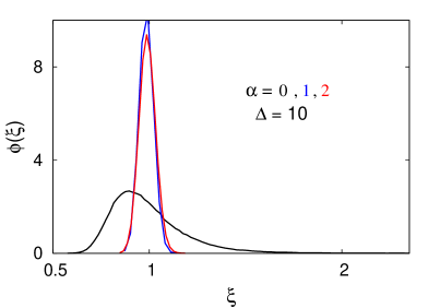
Figure 2: Distribution $\phi(\xi)$ of the relative amplitude $\overline{\delta^{2}(\Delta)}\Big{/}\left<\overline{\delta^{2}(\Delta)}\right>$ of the time averaged MSD traces for SBM processes with different scaling exponents $\alpha$ as indicated in the panels. As expected, the spread grows and the distribution becomes more leptokurtic at longer lag times $\Delta$. For progressively larger values of the scaling exponent $\alpha$ the spread of time averaged MSD decreases but stays asymmetric with a longer tail at larger $\overline{\delta^{2}}$ values. In particular, for $\alpha=1$ and 2 the shape is almost indistinguishable at $\Delta=10$, see the bottom right panel. The trace length is $T=10^{4}$ and the number of traces used for averaging is $10^{3}$.

3 Ergodicity breaking of non-ageing scaled Brownian motion

3.1 General expression for the ergodicity breaking parameter

Analytically, the derivation of the EB parameter for SBM involves the evaluation of the fourth order moment of the time averaged MSD,

$$\left<\left(\overline{\delta^{2}(\Delta)}\right)^{2}\right>=\frac{1}{T-\Delta}\int\limits_{0}^{T-\Delta}dt_{1}\int\limits_{0}^{T-\Delta}dt_{2} \left<\Big{(}x^{2}(t_{1}+\Delta)-x(t_{1}))^{2}\right.$$ (13)

$$\left.\times(x^{2}(t_{2}+\Delta)-x(t_{2})\Big{)}^{2}\right>.$$

We use the fundamental property of SBM that

$$\left<x(t_{1})x(t_{2})\right>=\left<x^{2}(\mathrm{min}\{t_{1},t_{2}\})\right>,$$ (14)

and the Wick-Isserlis theorem for the fourth order correlators [48]. We then obtain the nominator $\mathcal{N}$ of the EB parameter of equation (8)

$$\mathcal{N}(\Delta) = \left<\left(\overline{\delta^{2}(\Delta)}\right)^{2}\right>-\left<\overline{\delta^{2}(\Delta)}\right>^{2}$$ (15)

$$= \frac{2}{(T-\Delta)^{2}}\int_{0}^{T-\Delta}dt_{1}\int_{0}^{T-\Delta}dt_{2}\left<\Big{(}x(t_{1}+\Delta)-x(t_{1}))\right.$$

$$\hskip 113.81102pt\times\left.(x(t_{2}+\Delta)-x(t_{2})\Big{)}\right>^{2}.$$

Taking the averages by help of equation (14) we arrive at

$$\mathcal{N}(\Delta) = \frac{4}{(T-\Delta)^{2}}\int_{0}^{T-\Delta}dt_{1}\int_{t_{1}}^{T-\Delta}dt_{2}\left[\Big{<}x^{2}(t_{1}+\Delta)\Big{>}\right.$$ (16)

$$\hskip 113.81102pt\left.-\Big{<}x(t_{1}+\Delta)x(t_{2})\Big{>}\right]^{2}.$$

With the new variable $\tau^{\prime}=t_{2}-t_{1}$ (assuming $t_{2}>t_{1}$) and by changing the order of integration we find the expression

$$\mathcal{N}(\Delta) = \frac{4}{(T-\Delta)^{2}}\int_{0}^{\Delta}d\tau^{\prime}\int_{0}^{T-\Delta-\tau^{\prime}}dt_{1}\left[\Big{<}x^{2}(t_{1}+\Delta)\Big{>}\right.$$ (17)

$$\hskip 113.81102pt\left.-\Big{<}x^{2}(t_{1}+\tau^{\prime})\Big{>}\right]^{2}.$$

Now, the new variables $x^{\prime}=t_{1}/\Delta$ and $y^{\prime}=\tau^{\prime}/\Delta$ are introduced. Substituting equation (1) into equation(17) we obtain

$$\mathcal{N}(\Delta) = \frac{16K_{\alpha}^{2}\Delta^{2\alpha+2}}{(T-\Delta)^{2}}\int_{0}^{1}dy^{\prime}\int_{0}^{T/\Delta-1-y^{\prime}}dx^{\prime}$$ (18)

$$\times\left[(x^{\prime}+1)^{2\alpha}-2(x^{\prime}+1)^{\alpha}(x^{\prime}+y^{\prime})^{\alpha}+(x^{\prime}+y^{\prime})^{2\alpha}\right].$$

Splitting the double integral over the variable $x^{\prime}$ into an integral over a square region and a triangular region yields

$$\int_{0}^{1}dy^{\prime}\int_{0}^{T/\Delta-2}dx^{\prime}+\int_{0}^{1}dy^{\prime}\int_{T/\Delta-2}^{T/\Delta-1-y^{\prime}}dx^{\prime}$$

$$\hskip 51.21504pt=\int_{0}^{T/\Delta-2}dx^{\prime}\int_{0}^{1}dy^{\prime}+\int_{T/\Delta-2}^{T/\Delta-1}dx^{\prime}\int_{0}^{T/\Delta-1-x^{\prime}}dy^{\prime}.$$ (19)

From the double integrals from the power-law functions in equation (18), via equation (14) we compute the nominator as

$$\mathcal{N}(\Delta,\tau) = \frac{16K_{\alpha}^{2}\Delta^{2\alpha+2}}{(T-\Delta)^{2}}\left[\frac{(\tau-1)^{2\alpha+1}}{2\alpha+1}+\frac{(3\alpha+1)(\tau-1)^{2\alpha+2}}{2(\alpha+1)^{2}(2\alpha+1)}\right.$$ (20)

$$-\frac{2\tau^{\alpha+1}(\tau-1)^{\alpha+1}}{(\alpha+1)^{2}}+\frac{\tau^{2\alpha+2}}{2(\alpha+1)(2\alpha+1)}-\frac{(2\alpha^{2}+\alpha+1)}{2(\alpha+1)^{2}(2\alpha+1)}$$

$$\left.+\frac{2}{\alpha+1}\int_{0}^{\tau-1}dx^{\prime}~{}(x^{\prime})^{\alpha+1}(x^{\prime}+1)^{\alpha}\right],$$

in terms of the variable

$$\tau=\frac{T}{\Delta}.$$ (21)

The integral

$$I_{1}(\tau)=\int_{0}^{\tau-1}dx^{\prime}~{}(x^{\prime})^{\alpha+1}(x^{\prime}+1)^{\alpha}$$ (22)

remaining in the last term of this expression can, in principle, be represented in terms of the incomplete Beta-function. The denominator $\mathcal{D}(\Delta)$ of the EB parameter (8) is just the squared time averaged MSD given by equation (6). We thus arrive at the expression

$$\mathcal{D}(\Delta,\tau) = \left[\frac{2K_{\alpha}\Delta^{\alpha+1}}{(\alpha+1)(T-\Delta)}(\tau^{\alpha+1}-1-(\tau-1)^{\alpha+1})\right]^{2}.$$ (23)

Note that the double analytical integration of equation (9) in [24] via Wolfram Mathematica yields a result, that is indistinguishable from equation (20), as demonstrated by the blue dots in figure 3B.

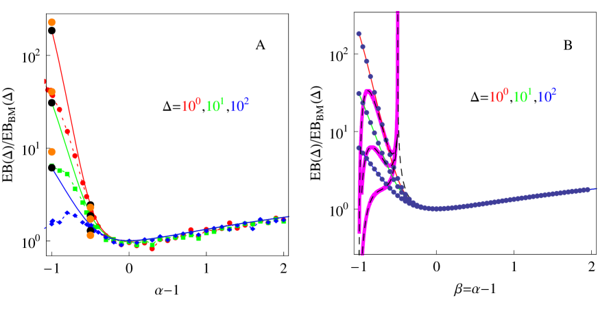
Figure 3: Ergodicity breaking parameter EB of non-ageing SBM. (A) Results of numerical simulations are depicted by the data points. The analytical results based on equations (20) and (23) are given by the solid coloured lines. Data points for different lag times are shown in different colours. The values of EB for ultraslow SBM (31) at $\alpha=0$ and at $\alpha=1/2$ given by equation (32) are shown as the bigger black bullets, computed for $\Delta=10^{0}$, $10^{1}$, and $10^{2}$. The larger orange bullets denote the same limits but without the additive constants to the leading functional dependencies with $\Delta/T$. Parameters: the trace length is $T=10^{4}$, the number of traces used for averaging at each $\alpha$ value is $N=10^{3}$. (B) Exact and approximate analytical results for EB. The red, green, and blue curves are the exact evaluations of equation (20). The dashed curve in the region $\alpha>1/2$ corresponds to equation (30) and the dashed curves for $0<\alpha<1/2$ are the results of [24]. The magenta curves in the region $0<\alpha<1/2$ are according to the analytical expansion (27) for given $\Delta$ values. The dark blue data points, coinciding with our exact result (20), follow from evaluating the double integral in equation (9) of [24] with Mathematica.

3.2 Expansions and Limiting Cases

We here consider some limiting cases of the EB parameter based on expressions (20) and (20). In the limit $\alpha=1$ and for $\Delta/T\ll 1$ the leading order expansion in terms of $\Delta/T$ turns into equation (9). As it should the SBM process reduces to the ergodic behaviour of standard Brownian motion.

3.2.1 The case $0<\alpha<1/2$.

The general expression for the behaviour of the EB parameter in the range $0<\alpha<1/2$ follows from equation (22) by help of the identity [equation (1.2.2.1) in Ref. [49]]

$$\int x^{p}(x+1)^{q}dx=\frac{x^{p+1}(x+1)^{q}}{p+q+1}+\frac{q}{p+q+1}\int x^{p}(x+1)^{q-1}dx,$$ (24)

that can be checked by straight differentiation. Performing this sort of partial integration three times we reduce the power of the integrand so that in the limit $\tau\to\infty$ the integral becomes a converging function. In the range $0<\alpha<1/2$ we the find exact expression

$$I_{1}(\tau) = \frac{(\tau-1)^{\alpha+2}\tau^{\alpha}}{2(\alpha+1)}+\frac{\alpha(\tau-1)^{\alpha+2}\tau^{\alpha-1}}{2(\alpha+1)(2\alpha+1)}+\frac{\alpha(\alpha-1)(\tau-1)^{\alpha+2}\tau^{\alpha-2}}{4\alpha(\alpha+1)(2\alpha+1)}$$ (25)

$$+\frac{\alpha(\alpha-1)(\alpha-2)}{4\alpha(\alpha+1)(2\alpha+1)}\times\int_{0}^{\tau-1}(x^{\prime})^{\alpha+1}(x^{\prime}+1)^{\alpha-3}dx^{\prime}.$$

The remaining converging integral can be represented in the limit $\Delta/T\ll 1$ via the Beta function: setting the upper integration limit $(\tau-1)\to\infty$ we obtain

$$\int_{0}^{\infty}(x^{\prime})^{\alpha+1}(x^{\prime}+1)^{\alpha-3}dx^{\prime}=B(\alpha+2,1-2\alpha).$$ (26)

Then we arrive at the following scaling law for the EB parameter,

$$\mathrm{EB}(\alpha,\Delta)\sim 4C(\alpha)\left(\frac{\Delta}{T}\right)^{2\alpha},$$ (27)

where the coefficient is given by

$$C(\alpha)=\frac{(1-\alpha)(2-\alpha)B(\alpha+2,1-2\alpha)-(2\alpha^{2}+\alpha+1)}{2(\alpha+1)^{2}(2\alpha+1)}.$$ (28)

The scaling form of EB versus $(\Delta/T)$ of equation (27) coincides with that proposed in reference [24], and it is indeed valid for vanishing $\Delta/T$ and scaling exponents not too close to $\alpha=0$ and $\alpha=1/2$, see below. We find in addition that in the region $0<\alpha\lesssim 1/2$ the EB parameter of the SBM process becomes a sensitive function of the lag time $\Delta$, as shown in figure 3A, both from our theoretical results and computer simulations. This means that no universal rescaled variable $\Delta/T$ exists, as is the case for standard Brownian motion.

The asymptote (27) agrees with the result (10) in [24] in the range $0<\alpha<1/2$ of the scaling exponent and for infinitely large values $\tau$. Equation (28) above provides an explicit form for the prefactor. In figure 3B the approximate expansion (27) is shown as magenta curve. At realistic values $\Delta/T$ the asymptote (27) agrees neither with our exact expression (20) nor with the simulation data. As this demonstrates the exact expression (20) needs to be used a forteriori. The main reason is the finite $\tau$ value used in the simulations: for very small $\Delta/T$ equation (27) describes the exact result (20) significantly better (not shown). We note that away from the critical points at $\alpha=0$ and $\alpha=1/2$, equation (27) returns zero and infinity, respectively (magenta curves in figure 3B). At these points special care is required when computing $I_{1}$ in equation (25), as discussed below.

3.2.2 The case $\alpha>1/2$.

For values $\alpha>1/2$ of the scaling exponent in the limit of small $\Delta/T$ the denominator (23) becomes $\mathcal{D}(\tau)\simeq 4\tau^{2\alpha}$. Note that here we need to include two more iterations of the integral in the last term of equation (25) by using equation (24). Then we arrive at a new integral term that is converging at $\tau\to\infty$. Thus the nominator (20)—after cancellation of the first three orders in the expansion in terms of large $\tau$—yields to leading order $\mathcal{N}(\tau)\simeq 16\alpha^{2}\tau^{2\alpha-1}/[3(2\alpha-1)]$.

From the exact expression (20) by using the integration formula (24) four times, we find the exact representation

$$I_{1}(\tau) = \frac{(\tau-1)^{\alpha+2}\tau^{\alpha}}{2(\alpha+1)}+\frac{\alpha(\tau-1)^{\alpha+2}\tau^{\alpha-1}}{2(\alpha+1)(2\alpha+1)}+\frac{\alpha(\alpha-1)(\tau-1)^{\alpha+2}\tau^{\alpha-2}}{4\alpha(\alpha+1)(2\alpha+1)}$$ (29)

$$+\frac{\alpha(\alpha-1)(\alpha-2)(\tau-1)^{\alpha+2}\tau^{\alpha-3}}{4\alpha(\alpha+1)(2\alpha+1)(2\alpha-1)}$$

$$+\frac{\alpha(\alpha-1)(\alpha-2)(\alpha-3)}{4\alpha(\alpha+1)(2\alpha+1)(2\alpha-1)}\times\int_{0}^{\tau-1}(x^{\prime})^{\alpha+1}(x^{\prime}+1)^{\alpha-4}dx^{\prime}.$$

From this expression the leading term with the divergence at $\alpha=1/2$ is written explicitly and the remaining integral is converging only then. Plugging this expression into equations (20) and (23) and keeping terms of order $\tau^{2\alpha-1}$ in the limit $\tau\gg 1$ we recover the result of [24] given by equation (30), again valid in the range $\alpha>1/2$. Note that the divergence in the denominator of the last term in $I_{1}$ in equation (29) is compensated by the proper expansion of the remaining integral in $I_{1}$ in the limit of large values of $\tau$ for $\alpha>1/2$, see below.

The EB parameter then scales as

$$\lim_{\Delta/T\to 0}\mathrm{EB}(\Delta)\sim\frac{4}{3}\frac{\alpha^{2}}{2\alpha-1}\frac{\Delta}{T}.$$ (30)

This result coincides with expression (10) in [24] in the range $\alpha>1/2$. As mentioned already, special care is needed near the critical point $\alpha=1/2$. Equation (30) implies that SBM is an ergodic process, with the EB parameter scaling strictly linearly with $\Delta/T$ as in relation (9) for Brownian motion, however, with an $\alpha-$dependent prefactor of the form $\alpha^{2}/(2\alpha-1)$. In contrast to subdiffusive CTRW processes [4, 40] and heterogeneous diffusion processes [21] the EB parameter for Brownian motion converges to zero and thus for sufficiently long measurement times the result of time averaged observables become reproducible.

3.2.3 The case $\alpha=0$

Now let us focus on the critical points $\alpha=0$ and $\alpha=1/2$ in detail. At $\alpha\to 0$ the EB parameter of the ultraslow SBM process [36] can be obtained from equation (20). To this end we first expand result (20) for small $\alpha$ using the identity $x^{\alpha}=e^{\alpha\log(x)}$. In the remaining integral $I_{1}$ in equation (22) we first expand the integrand in powers of small $\alpha$ and then integrate the expanded function in the limits $\int_{0}^{T-\Delta}dt$. The first two orders of the expansion in $\alpha$ in the nominator of EB disappear. Dividing the leading orders in $\alpha^{2}$ in the nominator and denominator of EB and expanding for short lag times $\Delta/T\ll 1$ afterwards to the leading order we find

$$\lim_{\Delta/T\to 0}\mathrm{EB}_{\mathrm{USBM}}(\Delta)\sim\frac{4(\pi^{2}/6-1)}{(\log[T/\Delta]+1)^{2}}.$$ (31)

This result was obtained from independent considerations for ultraslow SBM as equation (20) in [36]. Note the logarithmic rather than the linear dependence of EB on $\Delta/T$ in this case, stemming from the ultraslow logarithmic scaling of the MSD and the time averaged MSD with (lag) time.

3.2.4 The case $\alpha=1/2$

Similarly, to explore the limit $\alpha\to 1/2$ we first expand the exact result (20) for $\mathcal{N}(\Delta)$ in $\alpha$ around this point. In analogy to the case $\alpha=0$ we expand the integrand in $I_{1}$ in terms of powers of $(\alpha-1/2)$ and then perform the integration over $t$ from $0$ to $T-\Delta$. Dividing the expansion of the nominator (20) of EB, taken at $\alpha=1/2$ in the limit $\Delta/T\to 0$, by the leading order of the denominator (23) in the same limit—scaling as $4\tau$—we get

$$\lim_{\Delta/T\to 0}\mathrm{EB}_{\alpha=1/2}(\Delta)=\frac{\Delta}{3T}\Big{[}\log(T/\Delta)+2\log(2)-5/6\Big{]}.$$ (32)

The same expression can be obtained by expanding equation (25) valid in the region $0<\alpha<1/2$. Alternatively result (32) can be obtained from the exact expression (29) valid for $\alpha>1/2$. In this case, however, due to a pole at $\alpha=1/2$ one more order in the power expansion near $\alpha=1/2$ needs to be properly evaluated when expanding $I_{1}$. Then, the divergence in the denominator of the prefactor of the last term in equation (29) becomes eliminated and the EB parameter stays continuous as $\alpha\to 1/2$.

Compared to the case $\alpha=1$ of Brownian motion the result (32) for EB features a weak logarithmic dependence on $\Delta/T$. As expected the values of EB according to equation (32) are very close to the exact solution (20), as shown by the larger black bullets for $\alpha=1/2$ in figure 3A. Note that for finite $T/\Delta$ values the additional constants following the leading functional dependencies in equation (31) and equation (32) play a significant rôle, as seen in figure 3A. The agreement of these EB values with the exact predictions of equation (20) and computer simulations is particularly good for smaller $\Delta/T$ values, as expected based on the large $\tau$ expansions used in the derivation of equations (31) and (32).

3.3 Computer Simulations

We implement the same algorithms for the iterative computation of the particle displacement $x(t)$ as developed for the heterogeneous diffusion process [21] and the combined heterogeneous diffusion-scaled Brownian motion process [26]. We simulate the one dimensional overdamped Langevin equation

$$\frac{dx(t)}{dt}=\sqrt{2D(t)}\times\xi(t)$$ (33)

driven by the Gaussian white noise $\xi(t)$ of unit intensity and zero mean. At step $i+1$ the particle displacement is

$$x_{i+1}-x_{i}=\sqrt{2[D(t_{i})+C]}(y_{i+1}-y_{i}),$$ (34)

where the increments $(y_{i+1}-y_{i})$ of the Wiener process represent a $\delta$ correlated Gaussian noise with unit variance and zero mean. Unit time intervals separate consecutive iteration steps. To avoid a possible particle trapping at the pole of $D(t)$ we introduced the small constant $C=10^{-3}$ in analogy to the procedure for heterogeneous diffusion processes [21]. The initial position of the particle is $x_{0}=x(t=0)=0.1$.

Our simulations results shown in figure 3A confirm the validity of the general analytical expressions (20) and (23) making up the EB parameter in the whole range of the scaling exponent $\alpha$. We also find that the short lag time expansion (30) agrees well with the exact solution and simulations at $\alpha\gtrsim 1/2$ (figure 3B). In the range $\alpha\gtrsim 1/2$ the EB parameter for $\Delta/T\ll 1$ is nearly insensitive to the lag time and grows with $\alpha$ in accord with equation (30). In particular, the full analytical expression for EB (equations (20) and (23)) and the results of the simulations show no divergence at $\alpha=1/2$, in contrast to the approximate results of reference [24].

Figure 3A also shows the approximate EB values (31) for ultraslow SBM as well as EB at $\alpha=1/2$ from equation (32) indicated as larger points. These points are close to our predictions for SBM at $\alpha\to 0$, in particular, for small $\Delta/T$ values when the approximations used in deriving the corresponding equations are better satisfied. As the ratio $\Delta/T$ grows and the scaling exponent converges to zero, $\alpha\to 0$—indicating progressively slower diffusion—the results of our simulations start to deviate from the exact analytical results (20) and (23), as shown in figure 3. In this limit apparently better statistics are needed in the simulations.

In figure 4 we show that EB scales with the trace length $T$ approximately as $1/T^{2\alpha}$ for $0<\alpha<1/2$ and as $1/T$ for $\alpha>1/2$; compare to the results in figure 1 of reference [24].

Figure 4: EB parameter for non-ageing SBM versus trace length $T$. The solid lines represent the exact results according to equation (20). Parameters: $\Delta=10$ and $N=10^{3}$.

4 Ergodicity breaking of ageing scaled Brownian motion

We consider the ergodic properties of ageing SBM, where $t_{a}$ denotes the time span in between the initiation of the system and start of the measurement. The ergodicity breaking parameter is defined through the ageing time averaged MSD (compare equations (10) and (11)) as

$$\mathrm{EB}_{a}(\Delta)=\frac{\left\langle\overline{\delta^{2}_{a}(\Delta)}^{2}\right\rangle-\left\langle\overline{\delta^{2}_{a}(\Delta)}\right\rangle^{2}}{\left\langle\overline{\delta^{2}_{a}(\Delta)}\right\rangle^{2}}=\frac{\mathcal{N}_{a}(\Delta,\tau)}{\mathcal{D}_{a}(\Delta,\tau)}$$ (35)

For the numerator we find in full analogy to the non-ageing situation

$$\mathcal{N}_{a}(\Delta) = \frac{4}{(T-\Delta)^{2}}\int_{t_{a}}^{T+t_{a}-\Delta}dt_{1}\int_{t_{1}}^{T+t_{a}-\Delta}dt_{2}$$ (36)

$$\times\left[\left\langle x^{2}(t_{1}+\Delta)\right\rangle-\left\langle x(t_{1}+\Delta)x(t_{2})\right\rangle\right]^{2}.$$

Changing the variables as above for the non-ageing scenario, $\tau^{\prime}=t_{2}-t_{1}$, we switch the limits of integration using $t_{1}(\tau^{\prime})=T+t_{a}-\Delta-\tau^{\prime}$ and then split the integrals over $\tau^{\prime}$ to compute the pair correlators using the property (14). This yields the representation of the nominator of EB in terms of one-point averages only,

$$\mathcal{N}_{a}(\Delta) = \frac{4}{(T-\Delta)^{2}}$$ (37)

$$\times\int_{0}^{\Delta}d\tau^{\prime}\int_{t_{a}}^{T+t_{a}-\Delta-\tau^{\prime}}dt_{1}\Big{[}\left\langle x^{2}(t_{1}+\Delta)\right\rangle-\left\langle x^{2}(t_{1}+\tau^{\prime})\right\rangle\Big{]}^{2}.$$

We proceed by inserting the MSDs of equation (1) and arrive at

$$\mathcal{N}_{a}(\Delta) = \frac{16K_{\alpha}^{2}\Delta^{2\alpha+2}}{(T-\Delta)^{2}}\int_{0}^{1}dy^{\prime}\int_{{t_{a}}/{\Delta}}^{T/{\Delta}+t_{a}/{\Delta}-1-y^{\prime}}dx^{\prime}$$ (38)

$$\times\Big{[}(x^{\prime}+1)^{2\alpha}-2(x^{\prime}+1)^{\alpha}(x^{\prime}+y^{\prime})^{\alpha}+(x^{\prime}+y^{\prime})^{2\alpha}\Big{]}.$$

Changing the order of integration and splitting the integral over $x^{\prime}$ we get in terms of the variables $\tau=T/\Delta$ and

$$\tau_{a}=\frac{t_{a}}{\Delta}$$ (39)

that

$$\mathcal{N}_{a}(\Delta,\tau) = \frac{16K_{\alpha}^{2}\Delta^{2\alpha+2}}{(T-\Delta)^{2}}\int_{\tau_{a}}^{\tau+\tau_{a}-2}dx^{\prime}\int_{0}^{1}dy^{\prime}\Big{[}(x^{\prime}+1)^{2\alpha}-2(x^{\prime}+1)^{\alpha}(x^{\prime}+y^{\prime})^{\alpha}$$ (40)

$$+(x^{\prime}+y^{\prime})^{2\alpha}\Big{]}+\int_{\tau+\tau_{a}-2}^{\tau+\tau_{a}-1}dx^{\prime}\int_{0}^{\tau+\tau_{a}-1-x^{\prime}}dy^{\prime}$$

$$\times\Big{[}(x^{\prime}+1)^{2\alpha}-2(x^{\prime}+1)^{\alpha}(x^{\prime}+y^{\prime})^{\alpha}+(x^{\prime}+y^{\prime})^{2\alpha}\Big{]}.$$

Finally, taking the integrals in the nominator of EB for ageing SBM yields

$$\mathcal{N}_{a}(\Delta,\tau) = \frac{16K_{\alpha}^{2}\Delta^{2\alpha+2}}{(T-\Delta)^{2}}\left[\frac{(\tau+\tau_{a}-1)^{2\alpha+1}}{2\alpha+1}-\frac{(\tau_{a}+1)^{2\alpha+1}}{2\alpha+1}\right.$$ (41)

$$+\frac{(3\alpha+1)(\tau+\tau_{a}-1)^{2\alpha+2}}{2(2\alpha+1)(\alpha+1)^{2}}+\frac{(3\alpha+1)(\tau_{a}+1)^{2\alpha+2}}{2(2\alpha+1)(\alpha+1)^{2}}$$

$$+\frac{(\tau_{a})^{2\alpha+2}}{2(2\alpha+1)(\alpha+1)}$$

$$+\frac{(\tau+\tau_{a})^{2\alpha+2}}{2(2\alpha+1)(\alpha+1)}-\frac{2(\tau+\tau_{a})^{\alpha+1}(\tau+\tau_{a}-1)^{\alpha+1}}{(\alpha+1)^{2}}$$

$$\left.+\frac{2}{\alpha+1}\int_{\tau_{a}}^{\tau+\tau_{a}-1}dx^{\prime}~{}(x^{\prime})^{\alpha+1}(x^{\prime}+1)^{\alpha}\right].$$

Here we again denote

$$I_{1}(\tau,\tau_{a})=\int_{\tau_{a}}^{\tau+\tau_{a}-1}dx^{\prime}(x^{\prime})^{\alpha+1}(x^{\prime}+1)^{\alpha}.$$ (42)

The denominator of EB follows from the time averaged MSD (11), namely [26, 43]

$$\mathcal{D}_{a}(\Delta,\tau) = \left<\overline{\delta^{2}_{a}(\Delta)}\right>^{2}=\Big{(}\frac{2K_{\alpha}\Delta^{\alpha+1}}{(\alpha+1)(T-\Delta)}\Big{[}(\tau+\tau_{a})^{\alpha+1}-(\tau_{a}+1)^{\alpha+1}$$ (43)

$$-(\tau+\tau_{a}-1)^{\alpha+1}+\tau_{a}^{\alpha+1}\Big{]}\Big{)}^{2}.$$

The final EB breaking parameter (35) for ageing SBM turns into expression (20) for the non-ageing case, $\tau_{a}=0$.

In the limit of strong ageing, $\tau_{a}\gg T\gg\Delta$, the time averaged MSD scales as

$$\left<\overline{\delta^{2}_{a}(\Delta)}\right>\sim 2\alpha K_{\alpha}t_{a}^{\alpha-1}\Delta$$ (44)

and the nominator of EB grows as

$$\mathcal{N}_{a}(\Delta,\tau)\sim 16K_{\alpha}^{2}\Delta^{2\alpha}\tau^{-2}(\alpha^{2}\tau_{a}^{2\alpha-2}\tau/3)$$ (45)

to leading order in large $\tau_{a}$ values and long trajectories. Then, the ergodicity breaking parameter follows the Brownian law (9). This limiting behaviour is supported by the simulations of strongly ageing SBM shown in figure 5. Moreover, it is similar to that of ageing ultraslow SBM [36]. Physically, in the limit of long ageing times $\tau_{a}$ the diffusivity $D(t)$ changes only marginally on the time scale $T\ll t$ of the particle diffusion, so that the entire process stays approximately ergodic.

In the opposite limit of weak ageing, $\tau_{a}\ll T$, we observe that $\left<\overline{\delta^{2}_{a}(\Delta,\tau)}\right>\sim 2K_{\alpha}\Delta^{\alpha}(\tau^{\alpha-1}+\alpha\tau_{a}\tau^{\alpha-2})$, and the nominator of EB to leading order of short $\tau_{a}$ and long $T$ values produces $\mathcal{N}(\Delta,\tau)\sim 16K_{\alpha}^{2}\Delta^{2\alpha}\tau^{-2}(\alpha^{2}\tau^{2\alpha-1}/[3(2\alpha-1)])$. Consequently the EB parameter to leading order is independent of the ageing time $\tau_{a}$ and follows equation (30) as long as $\alpha>1/2$.

Figure 5 shows the simulations results based on the stochastic Langevin process of ageing SBM. We find that in the limit of strong ageing, consistent with our theoretical results the EB of ageing SBM indeed approaches the Brownian limit (9). For weak and intermediate ageing the general EB expression (41) is in good agreement with the simulations results, compare the data sets in figure 5. Finally figure 6 depicts the graph of EB versus ageing time explicitly, together with the theoretical results (41) and (43). We observe that EB decreases with the ageing time and this reduction is particularly pronounced for strongly subdiffusive SBM processes. The latter also feature some instabilities upon the numerical solution of the stochastic equation for long ageing times.

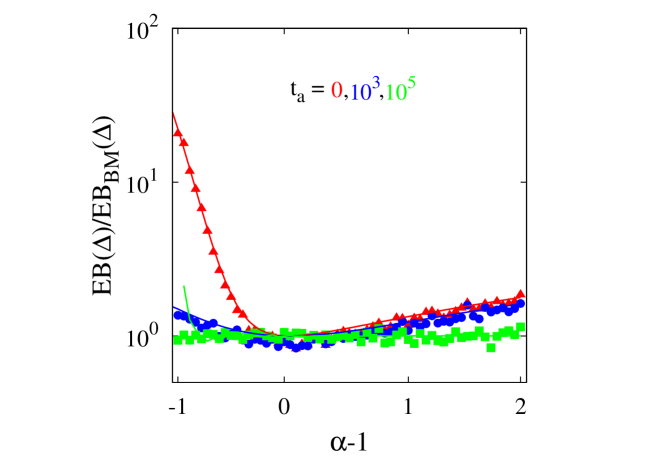
Figure 5: EB parameter for ageing SBM. Results of simulations are shown by the points and the analytical results (41) are represented by the solid lines of the corresponding colour. Parameters: $\Delta=10$, $T=10^{4}$, and $N=10^{3}$.

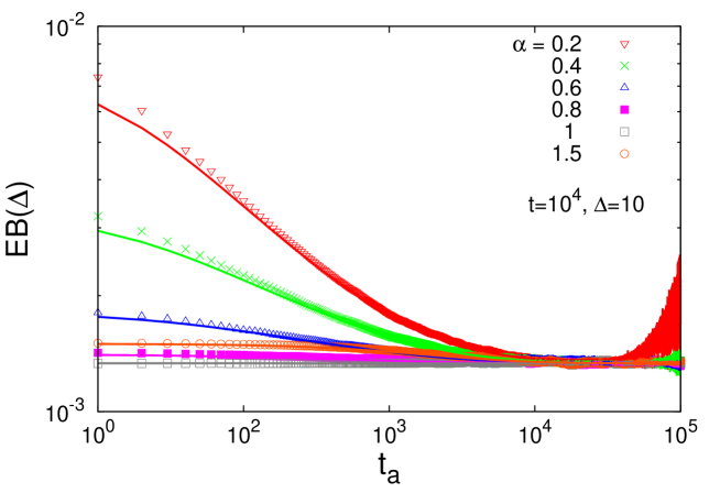
Figure 6: EB parameter for ageing SBM versus ageing time $t_{a}$. Analytical results (41) and (43) for different $\alpha$ values are represented by the solid lines. Some instabilities in the simulations are visible at long ageing times, in particular for small $\alpha$. Parameters: $\Delta=10$, $T=10^{4}$, and $N=10^{3}$.

5 Conclusions

We here studied in detail the ergodic properties of SBM with its power-law time dependent diffusivity $D(t)\simeq t^{\alpha-1}$. In particular, we derived the higher order time averaged moments and obtained the ergodicity breaking parameter of SBM, which quantifies the degree of irreproducibility of time averaged observables of a stochastic process. For the highly non-stationary, out-of-equilibrium SBM process we analysed the EB parameter with respect to the scaling exponent $\alpha$, the lag time $\Delta$, and the trace length $T$. We revealed a non-monotonic dependence $\mathrm{EB}(\alpha)$. In particular, we showed that there is no divergence at $\alpha=1/2$, in contrast to the approximate results of [24]. We also obtained a peculiar dependence for the EB dependence on the trace length $T$, $\mathrm{EB}(T)\sim 1/T^{2\alpha}$ for $0<\alpha<1/2$ and $\mathrm{EB}(T)\sim 1/T$ for $\alpha>1/2$, in agreement with [24]. We also obtained analytical and numerical results for EB for ageing SBM as function of the model parameters and the ageing time $t_{a}$.

Our exact analytical results are fully supported by stochastic simulations. We find that over the range $\alpha\gtrsim 1/2$ and for $\Delta/T\ll 1$ the EB dependence on the lag time and trace length involves the universal variable $1/\tau=\Delta/T$, as witnessed by equation (30). For arbitrary lag times and trace lengths the general result for ageing and non-ageing SBM are, however, more complex, see equations (20) and (41). These are the main results of the current work. For strongly subdiffusive SBM in the range of exponents $0<\alpha\lesssim 1/2$ the ergodic properties are, in contrast, strongly dependent on the lag time $\Delta$. The correct limit of our exact result (20) was obtained for the EB parameter of ultraslow SBM with $\alpha\to 0$ and for SBM with exponent $\alpha=1/2$. Although EB has some additional logarithmic scaling at this point, it reveals no divergence as $\alpha=1/2$ is approached.

We are confident that the strategies for obtaining higher order time averaged moments developed herein will be useful for the analysis of other anomalous diffusion processes, in particular for the analysis of finite time corrections of EB for fractional Brownian motion [45] or for processes with spatially and temporally random diffusivities [50, 51].

References

References

- [1] J.-P. Bouchaud and A. Georges, Phys. Rep. 195, 127 (1990).
- [2] R. Metzler and J. Klafter, Phys. Rep. 339, 1 (2000); J. Phys. A 37, R161 (2004).
- [3] F. Höfling and T. Franosch, Rep. Prog. Phys. 76, 046602 (2013).
- [4] R. Metzler, J.-H. Jeon, A. G. Cherstvy, and E. Barkai, Phys. Chem. Chem. Phys. 16, 24128 (2014).
- [5] C. Bräuchle, D. C. Lamb, and J. Michaelis, Single Particle Tracking and Single Molecule Energy Transfer (Wiley-VCH, Weinheim, Germany, 2012); X. S. Xie, P. J. Choi, G.-W. Li, N. K. Lee, and G. Lia, Annu. Rev. Biophys. 37, 417 (2008).
- [6] K. Burnecki, E. Kepten, J. Janczura, I. Bronshtein, Y. Garini, and A. Weron, Biophys. J. 103, 1839 (2012); E. Kepten, I. Bronshtein, and Y. Garini, Phys. Rev. E 83, 041919 (2011); J.-H. Jeon, V. Tejedor, S. Burov, E. Barkai, C. Selhuber-Unkel, K. Berg-Sørensen, L. Oddershede, and R. Metzler, Phys. Rev. Lett. 106, 048103 (2011); S. M. A. Tabei, S. Burov, H. Y. Kim, A. Kuznetsov, T. Huynh, J. Jureller, L. H. Philipson, A. R. Dinner, and N. F. Scherer, Proc. Natl. Acad. Sci. USA 110, 4911 (2013); A. V. Weigel, B. Simon, M. M. Tamkun, and D. Krapf, Proc. Natl. Acad. Sci. USA 108, 6438 (2011); C. Manzo, J. A. Torreno-Pina, P. Massignan, G. J. Lapeyre, Jr., M. Lewenstein, and M. F. Garcia Parajo, Phys. Rev. X 5, 011021 (2015).
- [7] J. Szymanski and M. Weiss, Phys. Rev. Lett. 103, 038102 (2009); G. Guigas, C. Kalla, and M. Weiss, Biophys. J. 93, 316 (2007); W. Pan, L. Filobelo, N. D. Q. Pham, O. Galkin, V. V. Uzunova, and P. G. Vekilov, Phys. Rev. Lett. 102, 058101 (2009); J.-H. Jeon, N. Leijnse, L. B. Oddershede, and R. Metzler, New J. Phys. 15, 045011 (2013).
- [8] E. Yamamoto, T. Akimoto, M. Yasui, and K. Yasuoka, Scient. Rep. 4, 4720 (2014); G. R. Kneller, K. Baczynski, and M. Pasienkewicz-Gierula, J. Chem. Phys. 135, 141105 (2011); J.-H. Jeon, H. Martinez-Seara Monne, M. Javanainen, and R. Metzler, Phys. Rev. Lett. 109, 188103 (2012).
- [9] A. Godec, M. Bauer, and R. Metzler, New J. Phys. 16, 092002 (2014); L.-H. Cai, S. Panyukov, and M. Rubinstein, Macromol. 48, 847 (2015); M. J. Skaug, L. Wang, Y. Ding, and D. K. Schwartz, ACS Nano 9, 2148 (2015).
- [10] Y. Meroz and I. M. Sokolov, Phys. Rep. 573, 1 (2015).
- [11] A. Caspi, R. Granek, and M. Elbaum, Phys. Rev. Lett. 85, 5655 (2000); N. Gal and D. Weihs, Phys. Rev. E 81, 020903(R) (2010); D. Robert, Th. H. Nguyen, F. Gallet, and C. Wilhelm, PLoS ONE 4, e10046 (2010); J. F. Reverey, J.-H. Jeon, M. Leippe, R. Metzler, and C. Selhuber-Unkel, Sci. Rep. 5, 11690 (2015).
- [12] E. Barkai, Y. Garini, and R. Metzler, Phys. Today 65(8), 29 (2012).
- [13] I. M. Sokolov, Soft Matter 8, 9043 (2012).
- [14] E. W. Montroll and G. H. Weiss, J. Math. Phys. 6, 167 (1965); H. Scher and E. W. Montroll, Phys. Rev. B 12, 2455 (1975).
- [15] J. H. P. Schulz, E. Barkai, and R. Metzler, Phys. Rev. Lett. 110, 020602 (2013); Phys. Rev. X 4, 011028 (2014).
- [16] A. V. Chechkin, M. Hofman, and I. M. Sokolov, Phys. Rev. E 80, 80, 031112 (2009); V. Tejedor and R. Metzler, J. Phys. A 43, 082002 (2010); M. Magdziarz, R. Metzler, W. Szczotka, and P. Zebrowski, Phys. Rev. E 85, 051103 (2012); J. H. P. Schulz, A. V. Chechkin, and R. Metzler, J. Phys. A 46, 475001 (2013).
- [17] J.-H. Jeon, E. Barkai, and R. Metzler, J. Chem. Phys. 139, 121916 (2013).
- [18] B. B. Mandelbrot and J. W. van Ness, SIAM Rev. 10, 422 (1968); A. M. Yaglom, Correlation theory of stationary and related random functions (Springer, Heidelberg, 1987).
- [19] P. Hänggi, Zeit. Physik B 31, 407 (1978); R. Kubo, Rep. Prog. Phys. 29, 255 (1966); I. Goychuk, Adv. Chem. Phys. 150, 187 (2012).
- [20] S. Havlin and D. Ben-Avraham, Adv. Phys. 36, 695 (1987); Y. Meroz, I. M. Sokolov, and J. Klafter, Phys. Rev. E 81, 010101(R) (2010); Y. Mardoukhi, J.-H. Jeon, and R. Metzler (unpublished).
- [21] A. G. Cherstvy, A. V. Chechkin, and R. Metzler, New J. Phys. 15, 083039 (2013); Phys. Chem. Chem. Phys. 15, 20220 (2013); Soft Matter 10, 1591 (2014); J. Chem. Phys. 142, 144105 (2015).
- [22] S. C. Lim and S. V. Muniandy, Phys. Rev. E 66, 021114 (2002).
- [23] A. Fulinski, Phys. Rev. E 83, 061140 (2011); J. Chem. Phys. 138, 021101 (2013); Acta Phys. Polon. 44, 1137 (2013).
- [24] F. Thiel and I. M. Sokolov, Phys. Rev. E 89, 012115 (2014).
- [25] J.-H. Jeon, A. V. Chechkin and R. Metzler, Phys. Chem. Chem. Phys. 16, 15811 (2014).
- [26] A. G. Cherstvy and R. Metzler, J. Stat. Mech. P05010 (2015).
- [27] T. Kühn, T. O. Ihalainen, J. Hyvaluoma, N. Dross, S. F. Willman, J. Langowski, M. Vihinen-Ranta, and J. Timonen, PLoS One 6, e22962 (2011); B. P. English, V. Hauryliuk, A. Sanamrad, S. Tankov, N. H. Dekker, and J. Elf, Proc. Natl. Acad. Sci. U. S. A. 108, E365 (2011).
- [28] E. Sykova and C. Nicholson, Physiol. Rev. 88, 1277 (2008).
- [29] D. S. Novikov, E. Fieremans, J. H. Jensen, and J. A. Helpern, Nature Phys. 7, 508 (2011).
- [30] D. S. Novikov, J. H. Jensen, J. A. Helpern, and E. Fieremans, Proc. Natl. Acad. Sci. U.S.A. 111, 5088 (2014).
- [31] M. J. Saxton, Biophys. J. 81, 2226 (2001).
- [32] G. Guigas, C. Kalla, and M. Weiss, FEBS Lett. 581, 5094 (2007); N. Periasmy and A. S. Verkman, Biophys. J. 75, 557 (1998); J. Wu and M. Berland, Biophys. J. 95, 2049 (2008); J. Szymaski, A Patkowski, J Gapiski, A. Wilk, and R. Holyst, J. Phys. Chem. B 110, 7367 (2006); E. B. Postnikov and I. M. Sokolov, Physica A 391, 5095 (2012).
- [33] L. F. Richardson, Proc. Roy. Soc. London Ser. A 110, 709 (1926).
- [34] G. K. Batchelor, Math. Proc. Cambridge Philos. Soc. 48, 345 (1952).
- [35] A. Bodrova, A. V. Chechkin, A. G. Cherstvy, and R. Metzler, E-print arXiv:1503.08125
- [36] A. Bodrova, A. V. Chechkin, A. G. Cherstvy, and R. Metzler, New J. Phys., at press.
- [37] L. Boltzmann, Vorlesungen über Gastheorie (J. A. Barth, Leipzip, 1898); P. Ehrenfest and T. Ehrenfest, Begriffliche Grundlagen der statistischen Auffassung in der Mechanik, in Enzyklopädie der Mathematischen Wissenschaften, vol. 4, subvol. 4, F. Klein and C. Müller, editors (B. G. Teubner, Leipzig, 1911); A. I. Khinchin, Mathematical foundations of statistical mechanics (Dover, New York, 1949).
- [38] Ya. G. Sinai, Theory Prob. Appl. 27, 256 (1982); G. Oshanin, A. Rosso, and G. Schehr, Phys. Rev. Lett. 110, 100602 (2013); D. S. Fisher, P. Le Doussal, and C. Monthus, Phys. Rev. E 64, 066107 (2001); A. Godec, A. V. Chechkin, E. Barkai, H. Kantz, and R. Metzler, J. Phys. A 47, 492002 (2014).
- [39] L. P. Sanders, M. A. Lomholt, L. Lizana, K. Fogelmark, R. Metzler, and T. Ambjörnsson, New J. Phys. 16, 113050 (2014).
- [40] Y. He, S. Burov, R. Metzler, and E. Barkai, Phys. Rev. Lett. 101, 058101 (2008).
- [41] I. M. Sokolov, E. Heinsalu, P. Hänggi, and I. Goychuk, Europhys. Lett. 86, 30009 (2009); M. J. Skaug, A. M. Lacasta, L. Ramirez-Piscina, J. M. Sancho, K. Lindenberg, and D. K. Schwartz, Soft Matter 10, 753 (2014); T. Albers and G. Radons, Europhys. Lett. 102, 40006 (2013).
- [42] D. Froemberg and E. Barkai, Phys. Rev. E 87, 030104(R) (2013); D. Froemberg and E. Barkai, Euro. Phys. J. B 86, 331 (2013); A. Godec and R. Metzler, Phys. Rev. Lett. 110, 020603 (2013).
- [43] H. Safdari, A. V. Chechkin, G. R. Jafari, and R. Metzler, Phys. Rev. E 91, 042107 (2015).
- [44] J.-P. Bouchaud, J. Phys. I 2, 1705 (1992); G. Bel and E. Barkai, Phys. Rev. Lett. 94, 240602 (2005); A. Rebenshtok and E. Barkai, Phys. Rev. Lett. 99, 210601 (2007).
- [45] W. Deng and E. Barkai, Phys. Rev. E 79, 01112 (2009).
- [46] S. M. Rytov, Yu. A. Kravtsov, and V. I. Tatarskii, Principles of statistical radiopysics 1: elements of random process theory (Springer, Heidelberg, 1987).
- [47] A. G. Cherstvy, A. V. Chechkin, and R. Metzler, J. Phys. A 47, 485002 (2014).
- [48] L. Isserlis, Biometrika 12, 134 (1918); G. C. Wick, Phys. Rev. 80, 268 (1950).
- [49] A. B. Prudnikov and Yu. A. Brychkov, Integrals and Series (Gordon and Breach, New York, 1986), Vol. 1.
- [50] P. Massignan, C. Manzo, J. A. Torreno-Pina, M. F. García-Parako, M. Lewenstein, and G. L. Lapeyre, Jr., Phys. Rev. Lett. 112, 150603 (2014).
- [51] M. V. Chubynsky and G. W. Slater, Phys. Rev. Lett. 113, 098302 (2014).