The Holographic Disorder-Driven Superconductor-Metal Transition

Abstract

We implement the effects of disorder on a holographic superconductor by introducing a random chemical potential on the boundary. We demonstrate explicitly that increasing disorder leads to the formation of islands where the superconducting order is enhanced and subsequently to the transition to a metal. We study the behavior of the superfluid density and of the conductivity as a function of the strength of disorder. We find explanations for various marked features in the conductivities in terms of hydrodynamic quasinormal modes of the holographic superconductors. These identifications plus a particular disorder-dependent spectral weight shift in the conductivity point to a signature of the Higgs mode in the context of disordered holographic superconductors. We observe that the behavior of the order parameter close to the transition is not mean-field type as in the clean case, rather we find robust agreement with $\exp(-A\,|T-T_{c}|^{-\nu})$, with $\nu=1.03\pm 0.02$ for this disorder-driven smeared transition.

Introduction: The suppression of conductivity due to disorder, known as Anderson localization, is one of the most striking transport phenomena that involves quantum behavior Anderson (1958). The application of localization ideas to superconductors was for a long time governed by Anderson’s theorem stating that nonmagnetic impurities have no significant effect on the superconducting transition since Cooper pairs are formed from time reversed eigenstates, which included disorder Anderson (1959). Anderson’s idea applies only to weakly disordered systems (with extended electronic states) and weak interactions; the role of interactions has been further discussed by Ma and Lee in Ma and Lee (1985). The mechanism put forward in Ma and Lee (1985) states that strong disorder gives rise to spatial fluctuations of the order parameter along with its suppression in comparison to its value in the clean system. The existence of spatial fluctuations of the order parameter has recently been corroborated and argued to be the central mechanism in the superconductor-insulator transition Galitski and Larkin (2001); Ghosal et al. (1998). Various experiments have indicated that high-$T_{c}$ superconductors are intrinsically disordered Pan and et al. (2001); Renner and et al. (2002) emphasizing the need for a better understanding of the interplay between superconductivity, strong interactions and disorder. In this manuscript we tackle this interplay using holographic methods.

The Anti de Sitter/Conformal Field Theory (AdS/CFT) correspondence has already succeeded in constructing holographic versions of superconductors Hartnoll et al. (2008a, b) (for reviews see Hartnoll (2009); Horowitz (2011)). Some holographic models have been argued to be relevant to describe materials like the cuprates Hartnoll et al. (2010); Sachdev (2012) since their dynamics is believed to be largely governed by their proximity to a quantum critical point Sachdev (2011).

In previous work Arean et al. (2014a, b) we investigated mild disorder in holographic superconductors and found an enhancement of the superconducting order parameter. Other recent works studying disorder holographically include Zeng (2013); Hartnoll and Santos (2014); O’Keeffe and Peet (2015). Here we explore the regime of large disorder and provide a detailed description of the superconductor-metal transition. Although we work in a setup where the normal phase describes a metal, it is also possible to consider insulating setups through AdS/CFT Nishioka et al. (2010); Donos and Hartnoll (2013); Donos et al. (2014).

In this paper we report various properties of the superconducting transition including the averaged and spatially resolved behavior of the condensate, superfluid density and conductivity and provide an explanation in terms of the relevant hydrodynamic modes. We observe that the disorder-driven transition is smeared and the averaged order parameter (here the average $\langle\cdot\rangle$ is over the spatial coordinate or, equivalently, disorder realizations) vanishes very quickly as $\langle{\cal O}\rangle\sim\exp\left(-A|T-T_{c}|^{-\nu}\right)$; we find $\nu=1.03\pm 0.02$. We expect that our explicit result for this exponent will stimulate alternative approaches to disorder-driven transitions to provide a quantitative characterization of the transition.

Disordered holographic superconductor: To build a noisy holographic $s$-wave superconductor in 2+1 dimensions we consider, following Hartnoll et al. (2008a), the dynamics of a Maxwell field and a charged scalar in a fixed metric background:

$$S=\int d^{4}x\,\sqrt{-g}\left(-{1\over 4}F_{ab}\,F^{ab}-(D_{\mu}\Psi)(D^{\mu}\Psi)^{\dagger}-m^{2}\Psi^{\dagger}\Psi\right).$$

The system is studied on the Schwarzschild-$AdS_{4}$ metric:

$$ds^{2} = {1\over z^{2}}\left(-f(z)dt^{2}+{dz^{2}\over f(z)}+dx^{2}+dy^{2}\right),$$

$$f(z) = 1-z^{3}\,,$$ (1)

where we have set the radius of AdS, $R=1$, and the horizon at $z_{h}=1$. This system is dual to a 2+1 CFT living on the boundary of $AdS_{4}$, and the $U(1)$ gauge field realizes a conserved current. The temperature of the black hole is identified with that of the field theory, and by fixing the horizon radius we are making use of the rescaling symmetry of our theory to work in units of temperature. We take the following (consistent) Ansatz for the matter fields:

$$\Psi(x,z)=\psi(x,z)\,,\quad A=\phi(x,z)\,dt,$$ (2)

where $\psi(x,z)\in{\mathbb{R}}$. The resulting equations of motion read

$$\partial_{z}^{2}\phi+\frac{1}{f}\,\partial_{x}^{2}\phi-{2\psi^{2}\over z^{2}\,f}\,\phi=0\,,$$ (3)

$$\partial_{z}^{2}\psi+\frac{1}{f}\,\partial_{x}^{2}\psi+\left({f^{\prime}\over f}-{2\over z}\right)\partial_{z}\psi+\frac{1}{f^{2}}\left(\phi^{2}-{m^{2}\,f\over z^{2}}\right)\psi=0\,.$$

(4)

In what follows we choose the scalar mass $m^{2}=-2$, corresponding to a dual operator of conformal dimension $\Delta=2$.

The main rule for reading the AdS/CFT dictionary states that field theory information is extracted from the boundary values of the gravity fields. The UV ($z=0$) asymptotics of Eqs. (3,4) lead to

$$\phi(x,z)=\mu(x)+\rho(x)\,z+\phi^{(2)}(x)\,z^{2}+o(z^{3})\,,$$ (5)

$$\psi(x,z)=\psi^{(1)}(x)\,z+\psi^{(2)}(x)\,z^{2}+o(z^{3})\,,$$ (6)

where $\mu(x)$ and $\rho(x)$ correspond, in the dual field theory, to space-dependent chemical potential and charge density respectively. The functions $\psi^{(1)}(x)$ and $\psi^{(2)}(x)$ are identified, under the duality, with the source and VEV of an operator of dimension 2. Imposing $\psi^{(1)}(x)=0$ in Eq. (6) corresponds to spontaneous breaking of the $U(1)$ symmetry with order parameter ${\cal O}\propto\psi^{(2)}(x)$. In the IR $(z\sim z_{h}=1)$ regularity implies that $A_{t}$ vanishes at the horizon.

To mimic the choice of random on-site potential used originally by Anderson in Anderson (1958) we implement disorder by introducing a noisy chemical potential:

$$\mu(x) = \mu_{0}+{\mu_{0}\over 25}\,w\,\sum_{k=k_{0}}^{k_{*}}\,\cos(k\,x+\delta_{k})\,,$$ (7)

where $\delta_{k}$ is a random phase for each $k$, and $w$ is a free parameter that determines the strength of the disorder. Notice that the system is homogeneous along the remaining spacelike direction $y$. We discretize the space, and impose periodic boundary conditions in the $x$ direction, leading to $k$ with values:

$$k_{n}={2\pi\over L}\,(n+1)\quad{\rm with}\quad 0\leq n<N=\frac{k_{*}}{k_{0}}\,,$$ (8)

where $L$ is the length in the $x$ direction of our cylindrical space. Our noise is a truncated version of Gaussian white noise where the highest wave number $k_{*}$ takes the role of the inverse of the correlation length for the chemical potential. More details on the properties of this choice of disorder can be found in Arean et al. (2014b).

Summarizing, we think of $k_{0}$ as the inverse system size and of $k_{*}$ as the inverse correlation length, and we work in the regime $k_{0}/T\ll 1$. More precisely, for most of the simulations we take $L=20\pi$, and $k_{*}=1$, but we checked the stability of the results for lengths up to $L=80\pi$.

To find solutions describing disordered superconducting states we integrate the equations of motion (3, 4) for different realizations of disorder characterized by sets of the random phases $\delta_{k}$. We define the expectation values for the different observables by averaging over different realizations. Typical plots correspond to about fifty realizations.

The order parameter and superconducting islands: Let us focus on the behavior of the order parameter as a function of the chemical potential $\mu$ and the dimensionless strength of disorder $w$. We will pay special attention to the minimum of the condensate ${\cal O}_{\rm min}$ throughout the sample which we expect to be related with the DC conductivity.

In Arean et al. (2014a, b) it was shown that noise enhances the spatial average of the order parameter. However, already Ma and Lee found in Ma and Lee (1985) that strong disorder gives rise to spatial fluctuations of the order parameter along with its suppression in comparison with its value in the clean/homogeneous system. In Fig. 1 we plot the spatial dependence of the order parameter at a temperature $T=0.81T_{c}^{w=0}$, where $T_{c}^{w=0}$ is the homogeneous critical temperature. We find that for strong enough noise regions akin to islands appear in the system.

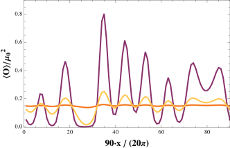
Figure 1: The condensate as a function of the coordinate $x$ for three realizations with strength $w=0.1,0.9,3,$ and the same set ${\delta_{k}}$ (orange, yellow and purple lines respectively), at a temperature $T=0.81T_{c}^{w=0}$. This plot shows the appearance of islands, that is, of spatial fluctuations in the condensate.

The enhancement of superconducting properties reported in Arean et al. (2014a, b) has some precedent in the condensed matter literature. The role of superconducting islands was already explicitly mentioned in Spivak and Zhou (1995), and further analyzed in Galitski and Larkin (2001). In that work it was shown that for each realization of disorder, there are spatial regions where the local upper critical field exceeds the system-wide average value. These regions form superconducting islands weakly coupled via the Josephson effect. At low temperatures, proximity coupling is long ranged and, thus, global superconductivity may be established in the system. Similar arguments were also advanced in Ghosal et al. (1998). We see that precisely this mechanism seems to be at play in our holographic model.

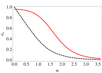
Figure 2: Superfluid density, $n_{s}$ (solid line) and minimum of the condensate, ${\cal O}_{\rm min}$ (dashed line), as a function of disorder, $w$, for $T/T_{c}^{w=0}=0.81$. The value of ${\cal O}_{\rm min}$ has been normalized to unity at $w=0$.

To characterize the possible appearance of islands we study the minimum of the condensate ${\cal O}_{\rm min}$ for different values of the parameters that characterize the system. In Fig. 2 we plot ${\cal O}_{\rm min}$ (dashed line) as function of the disorder strength $w$ at constant temperature $T=0.81T_{c}^{w=0}$. This figure shows that ${\cal O}_{\rm min}$ is a holographic version of the original suggestion of Ma and Lee Ma and Lee (1985) that strong disorder gives rise to spatial fluctuations of the order parameter along with its suppression in comparison with its value in the clean/homogeneous system. Moreover, for large values of the disorder strength we observe an exponential tail for ${\cal O}_{\rm min}$. This means that we have some leaking between islands of superfluid leading to a finite value of the condensate in between. We relate this to the fact that AdS suppresses large momentum contributions to the order parameter as reported in Arean et al. (2014a, b).

Conductivities: The holographic computation of conductivities requires the study of fluctuations on top of the background. Here we focus on the conductivity of the $U(1)$ broken superconducting phase, where the perturbations couple to the noise due to the nontrivial scalar field. Given the symmetries of the setup, there are two different conductivities one can study: the one in the direction parallel to the noise and that orthogonal to it. The orthogonal conductivity is insensitive to the disorder, and we thus focus on the parallel one.

To compute the electric conductivity we consider homogeneous perturbations of the gauge field oscillating with frequency $\omega$:

$$A_{\mu}=A_{\mu}^{(0)}(x,z)+a_{\mu}(x,z)\,e^{-i\omega\,t}\,,$$ (9)

and on the boundary ($z=0$) we impose $f_{ti}(x)=1$ (where $f_{\mu\nu}$ is the field strength of $a_{\mu}$, and $i$ runs over the spatial directions $x,y$), thus sourcing a constant electric field in the dual field theory. Then, following AdS/CFT, the conductivity is computed as

$$\sigma_{ii}(x)=\frac{\langle J_{i}\rangle}{E_{i}}=-\frac{i\partial_{z}a_{i}(x,z)}{\omega\,a_{i}(x,z)}\bigg{|}_{z\to 0}\,,$$ (10)

where there is no summation over $i$, and we impose ingoing boundary conditions for $a_{i}(x,z)$ at the horizon.

For the conductivity in the direction of the noise we must consider the linearized equations for the spatial component of the gauge field $a_{x}(x,z)$. Unfortunately, the $x$ dependence couples $a_{x}$ to the perturbation of the temporal component of the gauge field $a_{0}(x,z)$ and to the perturbations of the scalar field $\chi(x,z)+i\eta(x,z)$, and we must then solve the four coupled linear equations of motion (15). Interestingly, as we will show in Fig. 4, the fields $(\chi,\eta)$ show up as hydrodynamic modes in the computation of conductivities.

When looking for the low frequency behavior of the conductivity we find that, as in the homogeneous phase, we have a pole in the imaginary part of $\sigma$. This translates, through Kramers-Kronig rules, into a (numerically invisible) delta function in the real part, giving

$$\sigma\approx n_{s}\left(\pi\delta(\omega)+\frac{i}{\omega}\right)+\dots\,,$$ (11)

where $n_{s}$ is the superfluid density. Notice that for $\sigma_{xx}$, a near-boundary analysis of the equations of motion shows that, due to current conservation, the DC conductivity must be homogeneous, and therefore $n_{s}$ is a constant independent of $x$.

The dependence of the superfluid density on the strength of disorder is shown in Fig. 2, together with the evolution of the minimum value of the condensate. For low $w$, we verify that $n_{s}$ does not change much in total agreement with Anderson’s theorem even if we are describing a strongly coupled system. The persistence of the transport properties for weak disorder, even in strongly coupled systems, has been argued in the metal-insulator transition in Basko et al. (2006). Fig. 2 shows that for large $w$, both the superfluid density and the minimum of the condensate decay exponentially. This illustrates the disorder-driven transition to the normal (metallic) phase.

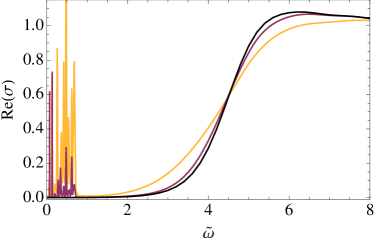
Figure 3: Real part of the AC conductivity for $T/T_{c}^{w=0}=0.45$. The black line corresponds to the homogeneous case, whereas the purple and yellow lines denote the disordered $w=1$ and $w=2.4$ cases respectively. The dimensionless frequency $\tilde{\omega}$ is proportional to $\omega/T$.

We present the real part of the AC conductivity in Fig. 3, comparing the homogeneous case with the results for two different values of the strength of disorder. The two key features absent in the homogeneous case are: the presence of resonances for small frequencies and a shift of the spectral weight at large frequencies. The small frequency resonances are a direct result of coupling of new fluctuating fields for an $x$-dependent chemical potential. These resonances can be understood as related to the holographic quasinormal modes studied in Amado et al. (2009, 2013) and shown to affect the conductivity at nonzero superfluid velocity in Amado et al. (2014). The shift in the spectral weight clearly depends on the strength of disorder, and we view it as evidence of the Higgs mode associated with the spontaneous breaking of the $U(1)$ symmetry Sherman and et al. (2015). The Higgs mode corresponds to oscillations of the modulus of the order parameter, and it is predicted Podolsky et al. (2011) to cause an excess of the electrical conductivity at sub-gap frequencies. In clean BCS superconductors the mass of the Higgs mode results in a gap of its contribution to the conductivity which is of the order of the BCS gap, and thus makes it difficult to detect the Higgs mode through its effect on the conductivity. However, it was shown in Gazit et al. (2013) that disorder suppresses that gap, giving rise to an observable excess of the AC conductivity at sub-gap frequencies with respect to the standard BCS prediction (based on the measurement of the energy gap of Cooper pairs) Sherman and et al. (2015). The excess observed in Sherman and et al. (2015) is qualitatively similar to what we observe in Fig. 3 at frequencies $2\lesssim\tilde{\omega}\lesssim 4$ where the conductivity of the disordered system (yellow line) is higher than that of the clean one (black line).

To verify that the small frequency resonances in the conductivity correspond to the gapless modes studied in Amado et al. (2013), we compute the effective velocity, $v_{s}$, of the first of these resonances assuming the dispersion relation

$$\omega=v_{s}(T,w)\,k\,,$$ (12)

and taking $k$ to be equal to $k_{0}$, where $k_{0}=2\pi/L$ is the smallest wave number in the sum (7). We then compare the evolution of $v_{s}$ with the temperature with the findings of Amado et al. (2013). The result is plotted in Fig. 4 which shows that $v_{s}(T,w)$ follows the standard temperature dependence discussed in Amado et al. (2009, 2013) (corresponding to the solid black line in the graphic). What is new in our case is its dependence on the disorder. For small temperatures the role of disorder is suppressed. For higher temperatures we see that $v_{s}$ decreases with increasing disorder strength except very near the critical temperature, Fig. 4.

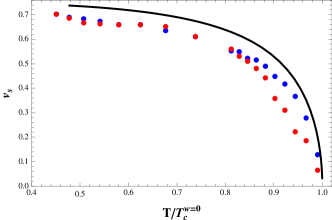
Figure 4: Effective velocity $v_{s}(T,w)$ corresponding to the first resonance of the conductivity for $w=0.1$ (blue dots) and $w=1$ (red dots). The black solid line presents the result of Amado et al. (2013) for the speed of sound of the sound mode in holographic superconductors.

Smeared phase transition: Finally, let us turn to the analysis of one of the most universal properties in phase transitions: the behavior of the order parameter close to the transition Wilson and Kogut (1974). As a first approach to disordered phenomena, the fate of a particular clean critical point under the influence of impurities is controlled by the Harris criterion Harris (1974) that generalizes the standard power-counting criterion to random couplings. As explained in Garcia-Garcia and Loureiro (2015) our chemical potential disordered along one dimension, and thus perfectly correlated along the remaining spatial direction, introduces relevant disorder. This places our setup in the class of systems where quenched disorder can lead to exotic critical points where the conventional power-law scaling does not hold McCoy (1969); Fisher (1992); Vojta (2003a). Moreover, in some cases disorder has been shown to cause the formation of rare regions undergoing a phase transition independently from the rest of the system. In terms of the average of the order parameter this results in a smeared phase transition characterized by an exponential scaling Vojta (2003b); Vojta and Schmalian (2005); Vojta (2006). One would expect the islands of conductivity that form in our system to play the role of these rare regions, and consequently to smear out the phase transition.

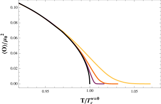
Figure 5: The disorder-driven transition is smeared. Plot of the spatial average of the condensate close to the critical temperature for $w=0$, 0.1, 0,2 and 0.4 (black, purple, orange, and yellow lines, respectively).

Fig. 5 shows the transition for the clean, homogeneous case Hartnoll et al. (2008b), and for three disordered cases $(w=0.1,0.2,0.4)$. We confirm that for the disordered transition the order parameter behaves as $\langle{\cal O}\rangle\sim\exp\left(-A|T-T_{c}|^{-\nu}\right)$ in Fig. 6. Notice that $T_{c}$ is different for each value of $w$, and is always higher than $T_{c}^{w=0}$. By taking the logarithmic derivative $\langle\mathcal{O}^{\prime}(T)\rangle/\langle\mathcal{O}(T)\rangle$, this figure shows linear fits that allow us to determine the exponent $\nu$, obtaining $\nu=1.03\pm 0.02$ independent of the disorder $w$. Explicitly, the fits in Fig. 6 are $y=-2.26-2.02x$ for $w=0.4$, $y=-3.13-2.01x$ for $w=0.2$, and $y=-4.21-2.06x$ for $w=0.1$, and notice that the slope of these fits corresponds to $-(\nu+1)$. The fits also show that the coefficient $A$ of the expression above increases with the disorder strength $w$, in agreement with the optimal fluctuation theory predictions Vojta (2003b, 2006). In particular, after assuming $\nu\approx 1$, these fits result in the following values of $A$: 0.01 at $w=0.1$, 0.04 at $w=0.2$, and 0.1 at $w=0.4$. The ranges of the fits, shown by solid black lines in Fig. 6, are determined on one side by the region where the condensate behaves as in the homogeneous case which as Fig. 5 shows is for temperatures around $.95T_{c}$. On the other side the bound arises from the numerical instability introduced by exponentially small values of the condensate. Notice that the points at temperatures above $T_{c}^{w=0}$ are rare, and many realizations are needed in order to have enough statistics to capture their behavior. Moreover, those points correspond to very low values of the condensate, and small errors in $\langle\mathcal{O}(T)\rangle$ affect strongly the value of $\langle\mathcal{O}^{\prime}(T)\rangle/\langle\mathcal{O}(T)\rangle$. Finally, one should notice that the UV cutoff $k_{*}$ in our disordered chemical potential bounds the disorder distribution. Consequently, one expects to find, as we do, a finite disordered critical temperature $T_{c}^{w}$ above which only the normal phase exists Vojta (2003b, 2006).

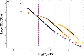
Figure 6: The disorder-driven transition is smeared. We plot $\log\left({1\over{\cal O}}\,{d{\cal O}\over dT}\right)$ versus $\log(T_{c}-T)$ for $w=0.1,0.2,0.4$ (purple, orange, and yellow respectively). The solid black lines denote linear fits to the data, and the vertical dashed lines indicate the critical temperature of the homogeneous case $T_{c}^{w=0}$.

Conclusions
Superconducting islands in holography: We argued that the formation of islands in the context of holographic disorder-driven superconductors is, as in experimental and numerical analyses, the central mechanism at play in the transition. This behavior is responsible for the enhancement of superconductivity reported in Arean et al. (2014a, b). The fact that the islands are coupled via the Josephson effect, as suggested originally in Galitski and Larkin (2001), causes the exponential decay in the tail of the superfluid density as shown in Fig. 2.

Disorder in strongly interacting systems: The interplay between disorder and interactions has been the subject of vigorous studies in the condensed matter literature initiated most recently by the work of Basko et al. Basko et al. (2006). In the series of works generated by Basko et al. (2006), (see for example Oganesyan and Huse (2007); Huse et al. (2014); Nandkishore and Huse (2014)) it is shown that for sufficiently strong disorder, weak interactions do not change the nature of the localized phase Chandran et al. (2015); Ros et al. (2015). The present work is in the complementary region, where interactions are strong to begin with, and disorder is increased. We have established that weak disorder does not destroy the holographic superconducting state, in particular, Fig. 2 shows that the superfluid density is largely unaffected for small disorder. Instead, for strong disorder the formation of islands suppresses the superfluid density driving the system to the normal phase.

Optical conductivity: We have studied the AC conductivity for disordered holographic superconductors, identifying the new low-frequency resonances with quasinormal modes of the holographic superconductor. Moreover, the conductivity displays a disorder-dependent shift of the spectral weight highly suggestive of a massive Higgs excitation. Strong experimental evidence in favor of a Higgs mode in strongly disordered superconductors close to the quantum phase transition has been recently reported in Sherman and et al. (2015).

The disorder-driven transition is smeared: We have shown that under the influence of disorder the superconductor-metal transition changes from power law, mean field to a smeared transition of the form $\exp(-A\,|T-T_{c}|^{-\nu})$, with $\nu=1.03\pm 0.02$. We hope that our results motivate other approaches to a quantitative description of this transition.

Future directions : Understanding the properties of conductivities in the language of modes helps us compare with more traditional condensed matter methods directly. Building a holographic disordered superconducting thin film will help us tackle the Higgs mode in the strongly disordered superconductor close to the quantum phase transition Sherman and et al. (2015). Ultimately, due to the universality of critical exponents Wilson and Kogut (1974), we hope that our holographic approach provides a direct path to disorder-driven critical exponents.

Acknowledgments It is a great pleasure to thank Nico Nessi for useful discussions. We thank the Galileo Galilei Institute for Theoretical Physics for hospitality and the INFN (Firenze) for partial support. D. A. is supported by GIF, grant 1156. We thank Zampolli for being a shelter of flavor. D.A. and I.S. thank the ICTP for hospitality at various stages of this collaboration. D.A. thanks the FROGS for unconditional support.

Appendix A Supporting material

Numerical stability: Given the aleatory nature of our calculation, in this appendix we show the stability of the result of the value of $\nu$ against the number of realizations. Namely, Fig. 7 shows that the result stabilizes as we increase the number of realizations of disorder, i.e. the number of times we generate a series of random phases, $\delta_{k}$ in Eq. (7). Most of our simulations for determining $\nu$ involve over 100 realizations.

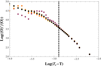
Figure 7: The condensates for $w=0.4$ with four different numbers of realizations: purple corresponds to 10 realizations, orange to 25, yellow to 75, and black to 150. Notice that except for the leftmost, high temperature, data points, the value of the condensate stabilizes for a number of realizations above 25.

Homogeneous versus smeared condensate: In Fig. 8 we show that the homogeneous transition follows a power law. We present it in the same plot as a smeared transition to illustrate how our numerical analysis distinguishes between the homogeneous and the disordered transition. Note that for an homogeneous condensate ${\cal O}_{h}=A_{h}|T-T_{c}|^{\beta}$, with $\beta=1/2$ Hartnoll et al. (2008b), hence one can write

$$\log\left(\frac{{\cal O}^{\prime}}{\cal O}\right)=-\log|T-T_{c}|+{\rm cons}\,,$$ (13)

while for the disordered case ${\cal O}=A_{s}\exp(-A|T-T_{c}|^{-\nu})$, and one has

$$\log\left(\frac{{\cal O}^{\prime}}{\cal O}\right)=-(\nu+1)\log|T-T_{c}|+{\rm cons}\,.$$ (14)

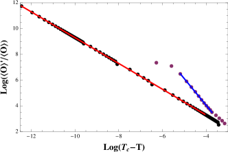
Figure 8: The homogeneous condensate (black dots) and the smeared condensate for $w=0.1$ (purple). The red, and blue lines correspond to the linear fits $y=-0.71-1.00x$, and $y=-4.21-2.06x$ respectively.

Equations of the perturbations: The equations of motion for the perturbations relevant for computing the electric conductivity read:

$$2\left(i\,\omega\,\eta+a_{0}\,\psi+2\,\phi\,\chi\right)\psi-z^{2}\left(f\,\partial_{zz}a_{0}+i\,\omega\,\partial_{x}a_{x}+\partial_{xx}a_{0}\right)=0\,,$$ (15a)

$$\frac{z^{2}}{f}\left(\omega^{2}\,a_{x}+f\,f^{\prime}\,\partial_{z}a_{x}+f^{2}\,\partial_{zz}a_{x}-i\,\omega\,\partial_{x}a_{0}\right)-2\left(\psi^{2}a_{x}-\psi\,\partial_{x}\eta+\partial_{x}\psi\,\eta\right)=0\,,$$ (15b)

$$-2\left(i\,\omega\,\eta+\psi\,a_{0}\right)\phi-z^{2}\phi^{2}\,\chi+\left(-z^{2}\,\omega^{2}+m^{2}\,f\right)\chi-z\,f\left(-2\,f\,\partial_{z}\chi+z\,f^{\prime}\,\partial_{z}\chi+z\,f\,\partial_{zz}\chi+z\,\partial_{xx}\chi\right)=0\,,$$ (15c)

$$\left[z^{2}\left(\omega^{2}+\phi^{2}\right)-m^{2}\,f\right]\eta-2\,x\,f^{2}\,\partial_{z}\eta+z^{2}\left[-i\,\omega\,a_{0}\,\psi-2\,i\,\omega\phi\,\chi+f\left(f^{\prime}\,\partial_{z}\eta+f\,\partial_{zz}\eta-\psi\,\partial_{x}a_{x}-2\,a_{x}\,\partial_{x}\psi+\partial_{xx}\eta\right)\right]=0\,,$$ (15d)

subject to the constraint:

$$-i\,z^{2}\,\omega\,\partial_{z}a_{0}+f\left(2\,\psi\,\partial_{z}\eta-2\,\eta\,\partial_{z}\psi-z^{2}\,\partial_{xz}a_{x}\right)=0\,.$$ (16)

References

- Anderson (1958) P. Anderson, Phys.Rev. 109, 1492 (1958).
- Anderson (1959) P. Anderson, Journal of Physics and Chemistry of Solids 11, 26 (1959), ISSN 0022-3697.
- Ma and Lee (1985) M. Ma and P. A. Lee, Phys. Rev. B 32, 5658 (1985).
- Galitski and Larkin (2001) V. M. Galitski and A. I. Larkin, Phys. Rev. Lett. 87, 087001 (2001).
- Ghosal et al. (1998) A. Ghosal, M. Randeria, and N. Trivedi, Phys. Rev. Lett. 81, 3940 (1998).
- Pan and et al. (2001) S. H. Pan and et al., Nature 413, 282 (2001).
- Renner and et al. (2002) C. Renner and et al., Nature 416, 518 (2002).
- Hartnoll et al. (2008a) S. A. Hartnoll, C. P. Herzog, and G. T. Horowitz, Phys.Rev.Lett. 101, 031601 (2008a), eprint 0803.3295.
- Hartnoll et al. (2008b) S. A. Hartnoll, C. P. Herzog, and G. T. Horowitz, JHEP 0812, 015 (2008b), eprint 0810.1563.
- Hartnoll (2009) S. A. Hartnoll, Class.Quant.Grav. 26, 224002 (2009), eprint 0903.3246.
- Horowitz (2011) G. T. Horowitz, Lect.Notes Phys. 828, 313 (2011), eprint 1002.1722.
- Hartnoll et al. (2010) S. A. Hartnoll, J. Polchinski, E. Silverstein, and D. Tong, JHEP 1004, 120 (2010), eprint 0912.1061.
- Sachdev (2012) S. Sachdev, Ann.Rev.Condensed Matter Phys. 3, 9 (2012), eprint 1108.1197.
- Sachdev (2011) S. Sachdev, Quantum phase transitions (Cambridge University Press, Cambridge, 2011), second ed. ed., ISBN 9780521514682.
- Arean et al. (2014a) D. Arean, A. Farahi, L. A. Pando Zayas, I. Salazar Landea, and A. Scardicchio, Phys.Rev. D89, 106003 (2014a), eprint 1308.1920.
- Arean et al. (2014b) D. Arean, A. Farahi, L. A. Pando Zayas, I. S. Landea, and A. Scardicchio (2014b), eprint 1407.7526.
- Zeng (2013) H. B. Zeng, Phys.Rev. D88, 126004 (2013), eprint 1310.5753.
- Hartnoll and Santos (2014) S. A. Hartnoll and J. E. Santos, Phys.Rev.Lett. 112, 231601 (2014), eprint 1402.0872.
- O’Keeffe and Peet (2015) D. K. O’Keeffe and A. W. Peet (2015), eprint 1504.03288.
- Nishioka et al. (2010) T. Nishioka, S. Ryu, and T. Takayanagi, JHEP 1003, 131 (2010), eprint 0911.0962.
- Donos and Hartnoll (2013) A. Donos and S. A. Hartnoll, Nature Phys. 9, 649 (2013), eprint 1212.2998.
- Donos et al. (2014) A. Donos, B. Gout raux, and E. Kiritsis, JHEP 1409, 038 (2014), eprint 1406.6351.
- Spivak and Zhou (1995) B. Spivak and F. Zhou, Phys. Rev. Lett. 74, 2800 (1995).
- Basko et al. (2006) D. Basko, I. Aleiner, and B. Altshuler, Annals of Physics 321, 1126 (2006), ISSN 0003-4916.
- Amado et al. (2009) I. Amado, M. Kaminski, and K. Landsteiner, JHEP 0905, 021 (2009), eprint 0903.2209.
- Amado et al. (2013) I. Amado, D. Arean, A. Jimenez-Alba, K. Landsteiner, L. Melgar, et al., JHEP 1307, 108 (2013), eprint 1302.5641.
- Amado et al. (2014) I. Amado, D. Are n, A. Jim nez-Alba, K. Landsteiner, L. Melgar, et al., JHEP 1402, 063 (2014), eprint 1307.8100.
- Sherman and et al. (2015) D. Sherman and et al., Nature 11, 188 (2015).
- Podolsky et al. (2011) D. Podolsky, A. Auerbach, and D. P. Arovas, Phys. Rev. B 84, 174522 (2011), URL http://link.aps.org/doi/10.1103/PhysRevB.84.174522.
- Gazit et al. (2013) S. Gazit, D. Podolsky, A. Auerbach, and D. P. Arovas, Phys. Rev. B 88, 235108 (2013), URL http://link.aps.org/doi/10.1103/PhysRevB.88.235108.
- Wilson and Kogut (1974) K. Wilson and J. B. Kogut, Phys.Rept. 12, 75 (1974).
- Harris (1974) A. B. Harris, Journal of Physics C: Solid State Physics 7, 1671 (1974).
- Garcia-Garcia and Loureiro (2015) A. M. Garcia-Garcia and B. Loureiro (2015), eprint 1512.00194.
- McCoy (1969) B. M. McCoy, Physical Review Letters 23, 383 (1969).
- Fisher (1992) D. S. Fisher, Physical review letters 69, 534 (1992).
- Vojta (2003a) T. Vojta, Physical review letters 90, 107202 (2003a).
- Vojta (2003b) T. Vojta, Journal of Physics A: Mathematical and General 36, 10921 (2003b).
- Vojta and Schmalian (2005) T. Vojta and J. Schmalian, Physical Review B 72, 045438 (2005).
- Vojta (2006) T. Vojta, Journal of Physics A: Mathematical and General 39, R143 (2006).
- Oganesyan and Huse (2007) V. Oganesyan and D. A. Huse, Phys. Rev. B 75, 155111 (2007).
- Huse et al. (2014) D. A. Huse, R. Nandkishore, and V. Oganesyan, Physical Review B 90, 174202 (2014).
- Nandkishore and Huse (2014) R. Nandkishore and D. A. Huse, arXiv preprint arXiv:1404.0686 (2014).
- Chandran et al. (2015) A. Chandran, I. H. Kim, G. Vidal, and D. A. Abanin, Physical Review B 91, 085425 (2015).
- Ros et al. (2015) V. Ros, M. Mueller, and A. Scardicchio, Nuclear Physics B 891, 420 (2015).