Privacy-Preserving Nonlinear Observer Design Using Contraction Analysis

Abstract.

Real-time information processing applications such as those enabling a more intelligent infrastructure are increasingly focused on analyzing privacy-sensitive data obtained from individuals. To produce accurate statistics about the habits of a population of users of a system, this data might need to be processed through model-based estimators. Moreover, models of population dynamics, originating for example from epidemiology or the social sciences, are often necessarily nonlinear. Motivated by these trends, this paper presents an approach to design nonlinear privacy-preserving model-based observers, relying on additive input or output noise to give differential privacy guarantees to the individuals providing the input data. For the case of output perturbation, contraction analysis allows us to design convergent observers as well as set the level of privacy-preserving noise appropriately. Two examples illustrate the approach: estimating the edge formation probabilities in a dynamic social network, and syndromic surveillance relying on an epidemiological model.

1. Introduction

The possibility to analyze vast amounts of personal data capturing information about the activities of private individuals is a foundational principle behind many current technology-driven trends such as the “Internet of Things”, electronic biosurveillance systems, or developing an intelligent infrastructure enabling smart cities. In many respects however, the data collection practices envisioned to operate these systems often go against basic privacy rights [2]. Concerns about the acquisition and use of personal data by companies and governments, e.g., for potential price and service discrimination, are rising [3, 4, 5], and could lead to people rejecting these technologies despite their suggested benefits. Rigorous privacy-preserving data analysis methodologies are needed to support regulations and allow people to appropriately trade off the privacy risks they increasingly incur with the benefits they can expect in return.

Typically, large-scale monitoring and control systems only require aggregate statistics computed from personal data streams, e.g., a dynamic map showing road traffic conditions built from location traces sent by smartphones, or an estimate of power consumption in a neighborhood updated using smart meter data from individual homes. Aggregation is beneficial to privacy, but past examples have shown that it is not sufficient to a priori rule out the possibility of significant privacy breaches [6, 7, 8]. Privacy attacks are often linkage attacks, where some newly published information is combined with other available data to make new inferences about specific individuals, and predicting at system design time how such attacks could be carried out is difficult. Yet, as explained below, it is still possible to compute aggregate statistics with formal privacy guarantees for the individuals from whom the data originates, which could help alleviate some of the justified concerns and encourage wider adoption of certain pervasive sensing and control systems.

Various information theoretic definitions have been proposed to capture quantitatively the concept of privacy and are potentially applicable to the processing of data streams in real-time [9]. In this paper, we focus on the notion of differential privacy, which originates from the database and cryptography literature [10]. Intuitively, a differentially private mechanism publishes information about a dataset in a way that is not too sensitive to a single individual’s data. As a result, an individual receives a guarantee that by providing her data, she will not drastically change the ability of a third party to make new inferences about her. Previous work has considered the design of linear filters processing sensitive time series data with differential privacy guarantees [11, 12, 13, 14, 15, 16, 17]. The problem studied in this paper is that of designing privacy-preserving nonlinear model-based estimators, which to the best of our knowledge has not been studied in a general setting before. A convenient way of achieving differential privacy for an estimator is to bound its so-called sensitivity [10], a form of incremental system gain between the private input signals and the published output [15]. Various tools could be used for this purpose, and here we rely on contraction analysis [18, 19, 20, 21].

The rest of the paper is divided as follows. Section 2 presents the problem statement formally, provides a brief introduction to the notion of differential privacy, and describes and compares privacy-preserving data analysis mechanisms with input and output perturbations. In Section 3 we discuss some fundamental results in contraction analysis and present a type of “Input-to-State Stability” property of contracting systems similar to the one proved in [19] but stated here for discrete-time systems. This property is used in Section 4 to design differentially private observers with output perturbation. The methodology is illustrated via two examples involving the analysis of dynamic data originating from private individuals. In Section 5.1, we consider the problem of estimating link formation probabilities in a dynamic social network, with a nonlinear measurement model. In Section 5.2, we consider a nonlinear epidemiological model and design a differentially private estimator of the proportion of susceptible and infectious people in a population, assuming a syndromic data source.

Notation: In this paper, $\mathbb{N}:=\{0,1,\ldots\}$ denotes the set of non-negative integers. For $H:\mathsf{X}\to\mathsf{Y}$ a linear map between finite dimensional vector spaces $\mathsf{X}$ and $\mathsf{Y}$ equipped with the norms $|\cdot|_{\mathsf{X}}$ and $|\cdot|_{\mathsf{Y}}$ respectively, we denote by $\|H\|_{\mathsf{X}}^{\mathsf{Y}}$ its induced norm, so that $|Hx|_{\mathsf{Y}}\leq\|H\|_{\mathsf{X}}^{\mathsf{Y}}\,|x|_{\mathsf{X}}$, for all $x$ in $\mathsf{X}$. If $\mathsf{X}=\mathsf{Y}$ and both spaces are equipped with the same norm $|\cdot|_{\mathsf{X}}$, we simply write $\|\cdot\|_{\mathsf{X}}$. For $1\leq p<\infty$, the $p$-norm on $\mathbb{R}^{n}$, denoted $|\cdot|_{p}$, is defined as $|v|_{p}:=\left(\sum_{i=1}^{n}|v_{i}|^{p}\right)^{1/p}$, and $|v|_{\infty}:=\max_{1\leq i\leq n}|v_{i}|$. For $v=\{v_{k}\}_{k\in\mathbb{N}}$ a vector-valued discrete-time signal, where $v_{k}\in\mathbb{R}^{n}$ has components $\{v_{k,i}\}_{i=1}^{n}$, the $\ell_{p}$ signal norm is $\|v\|_{p}=\left(\sum_{k=0}^{\infty}\sum_{i=1}^{n}|v_{k,i}|^{p}\right)^{1/p}=\left(\sum_{k=0}^{\infty}|v|_{p}^{p}\right)^{1/p}$ for $1\leq p<\infty$, and $\|v\|_{\infty}=\sup_{k\geq 0}|v_{k}|_{\infty}$. We use $\text{diag}(v)$ to denote a diagonal matrix with the components of the vector $v$ on the diagonal. For $P$ a symmetric matrix, $P$ positive definite is denoted $P\succ 0$ and $P$ positive semidefinite is denoted $P\succeq 0$. For $P\succeq 0$, we denote its (unique) positive semi-definite square root as $P^{1/2}$, i.e., $P=P^{1/2}P^{1/2}$. For $P$, $Q$ symmetric matrices, $P\succeq Q$ means $P-Q\succeq 0$, and $P\preceq 0$ means $-P\succeq 0$. The expressions “if and only if” and “independent and identically distributed” are abbreviated as iff and iid respectively. $\mathcal{C}^{1}$ denotes the set of continuously differentiable functions. A class $\mathcal{K}$ function $\beta:\mathbb{R}_{+}\to\mathbb{R}_{+}$ is a strictly increasing continuous function such that $\beta(0)=0$.

2. Problem Statement

2.1. Observer Design

Consider the problem of estimating a discrete-time signal denoted $x:=\{x_{k}\}_{k\in\mathbb{N}}$, with $x_{k}\in\mathsf{X}=\mathbb{R}^{n}$ for some integer $n$, which represents an aggregate state for a population of privacy-sensitive individuals. For example, $x_{k}$ could be the density at period $k$ of drivers or pedestrians at a finite number of spatial locations, the proportion of individuals infected by a disease in a population, etc. We assume that $x_{k}$ cannot be perfectly observed, but that we can measure instead a privacy-sensitive discrete-time signal $\{y_{k}\}_{k\in\mathbb{N}}$, with $y_{k}\in\mathsf{Y}=\mathbb{R}^{m}$ for some integer $m$, for which we have a state-space model of the form

(2.1) $$x_{k+1} =f_{k}(x_{k})+w_{k},$$

(2.2) $$y_{k} =g_{k}(x_{k})+v_{k},$$

where $w_{k},v_{k}$ are noise signals capturing modeling errors, and $f_{k}$ and $g_{k}$ are $\mathcal{C}^{1}$ functions. Our aim is to publish an estimate $z_{k}$ of $x_{k}$, computed from $y_{k}$ by an observer of the following form [22]

(2.3) $$z_{k+1}=f_{k}(z_{k})+h_{k}(z_{k},y_{k}-g_{k}(z_{k})),$$

with, for each $k$ in $\mathbb{N}$, $h_{k}:\mathsf{X}\times\mathsf{Y}\to\mathsf{X}$ a $\mathcal{C}^{1}$ function such that $h_{k}(x,0)=0$. We initialize (2.3) with some estimate $z_{0}$ of $x_{0}$. Note that (2.3) could describe an observer for a model (2.1)-(2.2) that has already been transformed under a suitable change of coordinates to a form that facilitates observer design, e.g., an observability canonical form [23, 24]. With straightforward modifications to our arguments, the “prediction” form (2.3) could also be replaced by an observer using the most recent observations

$$z_{0} =\bar{z}_{0}+h_{0}(\bar{z}_{0},y_{0}-g_{k}(\bar{z}_{0})),\quad\text{for some estimate $\bar{z}_{0}$ of $x_{0}$},$$

(2.4) $$z_{k+1} =f_{k}(z_{k})+h_{k+1}(z_{k},y_{k+1}-g_{k}(f_{k}(z_{k}))),\;\text{for }k\geq 0.$$

In the applications discussed later in the paper, the signal $y_{k}$ is collected from privacy-sensitive individuals, hence needs to be protected, in a sense defined below. On the other hand, the model (2.1)-(2.3), i.e., the functions $f_{k}$, $g_{k}$ and $h_{k}$, is assumed to be publicly available, or at least potentially known to any adversary trying to make inferences about $y$ based on $z$. The data aggregator wishes to publicly release the signal $z$ produced by (2.3). However, since $z$ depends on the sensitive signal $y$, we only allow the release of an approximate version of $z$ carrying certain privacy guarantees, which are presented formally in the next subsection. As a result, it will emerge that the functions $h_{k}$ need to be carefully chosen to balance accuracy or convergence speed of the observer with the level of privacy offered.

Remark 1.

We do not provide here nor use any model of the noise signals $w$ and $v$ in (2.1), (2.2), which are simply introduced as a device to explain the discrepancy between any measured signal $y$ and the signals that can be predicted by a deterministic model $x_{k+1}=f_{k}(x_{k}),y_{k}=g_{k}(x_{k})$.

Remark 2.

More generally, we might just want to publish an output $\chi_{k}(x_{k})$, function of the state $x_{k}$. As explained below, this can be done by first obtaining a privacy-preserving estimate $\hat{x}$ of the signal $x$ and then publishing $\chi_{k}(\hat{x}_{k})$, relying on the fact that sound privacy guarantees such as differential privacy are preserved by the final transformation through $\chi_{k}$.

2.2. Differential Privacy

The published signal should provide an accurate estimate of $x$ under an additional constraint that is not satisfied a priori by $z$ from (2.3), aiming at preserving the privacy of the individuals from which the measured signal $y$ originates. More precisely, we impose that the published signal be differentially private [10], which requires adding artificial noise somewhere in the signal processing system to randomize the published output. A differentially private version of the observer (2.3) should produce a randomized output signal whose distribution is not too sensitive to certain variations associated with the effect of any individual’s data on the signal $y$, input of the observer. The formal definition of differential privacy is given in Definition 1 below and requires that we specify the type of variations in $y$ that should be hard to detect from the published output. This is done by defining a symmetric binary relation, called adjacency and denoted Adj, on the space of datasets $\mathsf{D}$ of interest, here the space of signals $y$, so that two adjacent input signals $y$ and $\tilde{y}$ should produce (randomized) output signals with similar distributions. It is possible to define different adjacency relations [15] to model different data analysis scenarios. In this paper, $y$ is assumed to represent a (possibly multi-dimensional) signal that already aggregates the data obtained from multiple users, e.g., $y_{k}$ at a particular time period $k$ could be the number of people waiting in a hospital emergency room, the total power consumption of a group of homes during that period, etc. We then consider in particular the following adjacency relations between signals

(2.5) $$\text{Adj}(y,\tilde{y})\text{ iff }\|y-\tilde{y}\|_{p}\leq B_{p},$$

for $p=1$ or $p=2$ and some given fixed constant $B_{p}>0$, as well as the more restrictive adjacency relation

(2.6) $$\text{Adj}(y,\tilde{y})\text{ iff }\exists k_{0}\geq 0\text{ s.t. }\begin{cases}y_{k}=\tilde{y}_{k},&k<k_{0}\\ |y_{k}-\tilde{y}_{k}|_{p}\leq K\alpha^{k-k_{0}},&k\geq k_{0},\end{cases}$$

where again $p=1$ or $p=2$ and $K>0$, $0\leq\alpha<1$ are given fixed constants. In other words, we aim at hiding deviations in the signal $y$ (e.g., due to the contribution of one individual to the signal) that are bounded in $p$-norm (relation (2.5)), or more explicitly that can start at any time $k_{0}$ but then subsequently decrease geometrically (relation (2.6)). Note that even the more restrictive condition (2.6) is much more general than the adjacency relation considered in some previous work on the design of a differentially private counter [11, 12, 14], where adjacent (scalar) signals can vary at a single time period by at most one. In comparison, the adjacency condition (2.6) greatly enlarges the set of signal deviations that can result from the presence of any individual and for which we provide guarantees (deviation at a single period is obtained for $\alpha=0$). We can now state the definition of a differentially private mechanism, i.e., of a randomized map from input to output signals.

Definition 1.

Let $\mathsf{D}$ be a space equipped with a symmetric binary relation denoted Adj, and let $(\mathsf{R},\mathcal{M})$ be a measurable space, where $\mathcal{M}$ is a given $\sigma$-algebra over $\mathsf{R}$. Let $\epsilon,\delta\geq 0$. A randomized mechanism $M$ from $\mathsf{D}$ to $\mathsf{R}$ is $(\epsilon,\delta)$-differentially private (for Adj) if for all $d,d^{\prime}\in\mathsf{D}$ such that $\text{Adj}(d,d^{\prime})$, we have

(2.7) $$\mathbb{P}(M(d)\in S)\leq e^{\epsilon}\mathbb{P}(M(d^{\prime})\in S)+\delta,\;\;\forall S\in\mathcal{M}.$$

If $\delta=0$, the mechanism is said to be $\epsilon$-differentially private.

This definition quantifies the admissible deviations for the output distribution of a differentially private mechanism, when a variation at the input satisfies the adjacency relation. Smaller values of $\epsilon$ and $\delta$ correspond to stronger privacy guarantees. In this paper, the space $\mathsf{D}$ was defined as the space of input signals $y$, the adjacency relation considered is (2.5) or (2.6), and the output space $\mathsf{R}$ is the space of output signals for the observer, here $\mathsf{X}^{\mathbb{N}}$ since we wish to estimate $x$. The problem is to publish an accurate estimate of the state $x$ while satisfying the property of Definition 1 for specified values of $\epsilon$ and $\delta$.

Remark 3.

Definition 1 depends on the choice of $\sigma$-algebra $\mathcal{M}$, which must contain enough sets $S$ to provide a meaningful differential privacy guarantee. The interested reader can find a discussion of measurability issues in a previous paper[15].

2.3. Sensitivity and Basic Differentially Private Mechanisms

Enforcing differential privacy can be done by randomly perturbing the published output of a system [10, 15], at the expense of its quality or utility. Hence, we are interested in evaluating as precisely as possible the amount of noise necessary to make a mechanism differentially private. For this purpose, the following quantity plays an important role.

Definition 2.

Let $q\geq 1$. The $\ell_{q}$-sensitivity of a system $G$ with $m$ inputs and $n$ outputs with respect to an adjacency relation Adj is defined by $\Delta_{q}G=\sup_{\text{Adj(u,u')}}\|Gu-Gu^{\prime}\|_{q}$.

In practice we are interested in the sensitivity of a system for the cases $q=1$ and $q=2$. The basic mechanisms of Theorem 1 below (with proofs and references in a previous paper[15]), can be used to produce differentially private signals. First, we need the following definitions. A zero-mean Laplace random variable with parameter $b$ has the probability density function $\exp(-|x|/b)/2b$, and its variance is $2b^{2}$. The $\mathcal{Q}$-function is defined as $\mathcal{Q}(x):=\frac{1}{\sqrt{2\pi}}\int_{x}^{\infty}e^{-\frac{u^{2}}{2}}du$. Then, for $\epsilon>0$, $0.5\geq\delta>0$, let $K=\mathcal{Q}^{-1}(\delta)$ and define $\kappa_{\delta,\epsilon}=\frac{1}{2\epsilon}(K+\sqrt{K^{2}+2\epsilon})$, which can be shown to behave roughly as $O\left(\sqrt{\ln(1/\delta)}/\epsilon\right)$.

Theorem 1.

Let $G$ be a system with $m$ inputs and $n$ outputs, and fix a relation Adj in Definition 2. The mechanism $Mu=Gu+w$, where all $w_{k,i},k\in\mathbb{N},1\leq i\leq n$, are independent Laplace random variables with parameter $b\geq(\Delta_{1}G)/\epsilon$, is $\epsilon$-differentially private for Adj. If $w$ is instead a white Gaussian noise such that the covariance matrix of each sample $w_{k}$ is $\sigma^{2}I_{n}$ with $\sigma\geq\kappa_{\delta,\epsilon}\,\Delta_{2}G$, then the mechanism is $(\epsilon,\delta)$-differentially private.

The mechanisms of Theorem 1 are called the Laplace and the Gaussian mechanism. One reason for introducing the Gaussian mechanism is that typically the $\ell_{2}$-sensitivity is smaller than its $\ell_{1}$ counterpart, which leads to lower noise levels if one can tolerate $\delta>0$ in the privacy guarantee.

2.4. Input and Output Perturbation

Theorem 1 says that we can obtain a differentially private signal at the output of a system $G$ by adding noise with standard deviation proportional to $\Delta_{1}G/\epsilon$ or to $\kappa_{\delta,\epsilon}\Delta_{2}G$. A very useful additional result stated here informally says that post-processing a differentially private signal without re-accessing the privacy-sensitive input signal does not change the differential privacy guarantee [15]. Now, the system $G$ in Theorem 1 can simply be the identity, with $\ell_{1}$- and $\ell_{2}$- sensitivity for the adjacency relation (2.6) equal to $K/(1-\alpha)$ and $K/\sqrt{1-\alpha^{2}}$ respectively (and $B_{1}$ and $B_{2}$ for (2.5)). This immediately gives a first possible design approach for our privacy-preserving observer, simply adding Laplace or Gaussian noise directly to the input signal $y$, see Fig. 1 a). The observer can then be designed according to any desired methodology, and should try to mitigate the effect of the artificial input noise, whose distribution is known, in addition to the usual measurement error. We call this design an input perturbation mechanism. Note that for $\alpha$ close to $1$, $1/\sqrt{1-\alpha^{2}}$ is significantly smaller than $1/(1-\alpha)$, so that if we are willing to accept some $\delta>0$ in the privacy guarantee and to use the $2$-norm on $\mathsf{Y}$ in the adjacency relation (2.6), we can obtain much better accuracy by using the $\ell_{2}$-sensitivity.

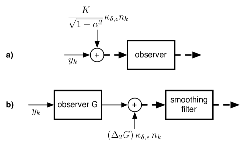
Figure 1. Gaussian mechanisms with input (a) and output (b) perturbation for the adjacency relation (2.6). $n_{k}$ represents a zero-mean standard white Gaussian noise with identity covariance matrix. Dashed lines represent a differentially private signal.

The input perturbation mechanism is attractive for its simplicity and might perform well, especially with low privacy level requirements (high $\epsilon$, $\delta$). In particular, the sensitive data can be made differentially private at the source, before sending it to any third party for processing. However, it can also potentially exhibit the following drawbacks. First, the noise added to $y$ might be unnecessarily large because it is not tailored to the task of estimating the state $x$ of the model (2.1)-(2.2), and does not take into account the temporal correlations between samples of the signal $y$ captured by this model. Significant noise at the input of the observer can also lead to poor performance, i.e., slow convergence and large errors in the state estimate, or even perhaps divergence of the estimate from the true state trajectory, since the convergence of nonlinear observers is often local. Second, characterizing the output error (state estimation error) due to the privacy-preserving noise requires understanding how this noise is transformed when passing through the nonlinear observer. In general, for nonlinear systems, the noise distribution at the output can become multimodal and non-zero mean, and hence the observer could produce a systematically biased estimate that could be hard to correct.

An alternative to input perturbation is the output perturbation mechanism shown on Fig. 1 b). In this case, following Theorem 1, a privacy-preserving noise signal proportional to the sensitivity of the observer $G$ is added at its output. Computing the sensitivity of $G$, or in practice upper bounding it, should be done as accurately as possible to reduce the conservatism of the approach. On the other hand the output noise does not impact any stability or bias analysis of the observer $G$. As discussed in more details in the following sections, we should then try to design an observer that has both good tracking performance for the state trajectory and low sensitivity, in order to minimize the level of privacy-preserving noise necessary at the output. These two desired properties are essentially in conflict. Fig. 1 b) shows that we can also add a terminal filter to smooth out the Laplace or Gaussian noise[25], although this can generally affect the transient performance of the overall system (e.g., its convergence speed). We do not discuss the design of a potential smoothing filter in this paper, except briefly in Subsection 5.1.

Example 1.

Consider the memoryless system $y_{k}\mapsto\phi(y_{k}):=y_{k}^{2}$, which could be a simple state estimator for a measurement model $y_{k}=\sqrt{x_{k}}$ in (2.2), which does not take the dynamics (2.1) into account. Consider the adjacency relation (2.6) for $\alpha=0$, so that we have a deviation at some (unknown) single time period $k_{0}$ of at most $K$ between adjacent signals $y_{k}$ and $\tilde{y}_{k}$. For the input perturbation scheme and the Gaussian mechanism, assuming for simplicity that $\kappa_{\delta,\epsilon}=1$, the signal $z_{k}=(y_{k}+K\xi_{k})^{2}=y_{k}^{2}+2Ky_{k}\xi_{k}+K^{2}\xi_{k}^{2}$ is differentially private when $\xi$ is a standard Gaussian white noise. The privacy-preserving noise at the input induces a systematic bias at the output between $z_{k}$ and $y_{k}^{2}$ equal to $\mathbb{E}[2Ky_{k}\xi_{k}+K^{2}\xi_{k}^{2}]=K^{2}$. Since $K$ is assumed publicly known, in this case the bias can be compensated and a better approximation of $\phi$ that is still differentially private is $z_{k}^{\prime}=(y_{k}+K\xi_{k})^{2}-K^{2}$. One can verify that the variance of the remaining error is $e^{\prime}_{k}=\mathbb{E}[(z_{k}^{\prime}-y_{k}^{2})^{2}]=4K^{2}y_{k}^{2}+2K^{4}$.

Suppose we know in addition that $y_{k}\in[0,1]$ for all $k\geq 0$. Then we can bound the sensitivity of the memoryless system as

(2.8) $$\Delta_{2}\phi=|y_{k_{0}}^{2}-\tilde{y}_{k_{0}}^{2}|=|y_{k_{0}}-\tilde{y}_{k_{0}}||y_{k_{0}}+\tilde{y}_{k_{0}}|\leq 2|y_{k_{0}}-\tilde{y}_{k_{0}}|\leq 2K.$$

Hence, the signal $z_{k}^{\prime\prime}=y_{k}^{2}+2K\xi_{k}$ is also differentially private and unbiased, with $\xi$ a standard white Gaussian noise as before. The variance of the error is $e_{k}^{\prime\prime}=\mathbb{E}[(z_{k}^{\prime\prime}-y_{k}^{2})^{2}]=4K^{2}$, which is smaller than the worst case value $4K^{2}+2K^{4}$ for $e_{k}^{\prime}$. However, $e_{k}^{\prime\prime}$ is larger than $e_{k}^{\prime}$ as soon as $y_{k}<\sqrt{1-K^{2}/2}$, the typical case since $K$ should be much less than $1$, otherwise both the input and output mechanisms essentially destroy the signal. The upper bound (2.8) on the sensitivity is conservative in order to be independent of the actual values of the sensitive signal $y$, which is necessary when Theorem 1 is used to provide a differential privacy guarantee.

In the rest of the paper we focus on the output perturbation mechanism of Fig. 1 b). There are two aspects to the differentially private observer design problem in this case. First, we need to enforce appropriate convergence of $z$ toward $x$, which is the observer design problem itself. Second, we also need to control and bound explicitly the magnitude of the changes in $z$ when the observer input changes from $y$ to an adjacent signal $\tilde{y}$, in order to apply Theorem 1 and set the output noise level providing the differential privacy guarantee. In this paper, both aspects of the problem are treated by using contraction analysis to design the observer as well as quantify its sensitivity to variations in the measured signal $y$. A motivation for this approach is the exponential convergence of trajectories of contractive systems toward each other, which provides a degree of robustness against input disturbances [18, 19, 26, 27] and, as a consequence, sensitivity bounds for variations in input data streams $y$. The next section provides some background on contraction analysis, necessary to describe our design approach in Section 4.

3. Contracting Systems

Contraction analysis is an “incremental” stability analysis methodology for dynamical systems emphasizing convergence of trajectories toward each other, popularized in particular by the work of Lohmiller and Slotine [18]. Earlier related work can also be found in the mathematics literature [28, 29]. Contraction and incremental stability analysis have seen significant developments in the past two decades [18, 21, 30, 31, 26, 32, 19, 20], and we refer the reader to the recent paper by Forni and Sepulchre [20] for a comparison of different variations that have emerged and additional references. The purpose of this section is to review some aspects of this methodology for discrete-time systems, which are not emphasized as much as continuous-time systems in the literature, and to state and prove some results that we rely on to design differentially private observers with output perturbation. Although these results could potentially be derived from the ideas presented in some of the references cited above, we provide here a self-contained discussion and in particular explicit bounds on distances between trajectories that are necessary to precisely set the level of privacy-preserving noise, since qualitative guarantees of incremental convergence are insufficient.

3.1. Basic Results

Consider a discrete-time system

(3.1) $$x_{k+1}=f_{k}(x_{k}),$$

with $f_{k}:\mathsf{X}\to\mathsf{X}$ a $\mathcal{C}^{1}$ function, for all $k\in\mathbb{N}$. Let us denote by $\phi(k;k_{0},x_{0})$ the value at time $k\geq k_{0}$ of the solution of (3.1) taking the value $x_{0}$ at time $k_{0}$. A forward invariant set for the system (3.1) is a set $C\subset\mathbb{\mathsf{missing}}X$ such that if $x_{0}\in C$, then for all $k_{0}$ and all $k\geq k_{0}$, $\phi(k;k_{0},x_{0})\in C$. Although we assume in this paper $\mathsf{X}=\mathbb{R}^{n}$, it is useful to introduce here some language from differential geometry and view $\mathsf{X}$ more generally as an $n$-dimensional differentiable manifold[33, 20]. For each point $x\in\mathsf{X}$, the tangent space to $\mathsf{X}$ at $x$, i.e., informally, the $n$-dimensional vector space of all tangent vectors to curves on $\mathsf{X}$ passing through $x$, is denoted $\mathsf{T}_{x}\mathsf{X}$. The tangent bundle of $\mathsf{X}$ is denoted $\mathsf{T}\mathsf{X}:=\cup_{x\in\mathsf{X}}\{x\}\times\mathsf{T}_{x}\mathsf{X}$, and is equipped with a time-varying family of norms $|\cdot|_{[x,k]}$, smoothly varying with $x$, so that $|\cdot|_{[x,k]}$ is a norm on $\mathsf{T}_{x}\mathsf{X}$, for all $k\in\mathbb{N}$. For each $x,\tilde{x}\in\mathsf{X}$, let $\Gamma(x,\tilde{x})$ be the set of piecewise $\mathcal{C}^{1}$ curves joining $x$ and $\tilde{x}$, i.e., functions $\gamma:[0,1]\to\mathsf{X}$ with $\gamma(0)=x$, $\gamma(1)=\tilde{x}$. We define the (time-varying) length of such a curve $\gamma$ by

$$L_{k}(\gamma)=\int_{0}^{1}|\gamma^{\prime}(r)|_{[\gamma(r),k]}dr,$$

where $\gamma^{\prime}(r):=\frac{d\gamma}{dr}(r)$. We then have a notion of (time-varying) geodesic distance on $\mathsf{X}$, defined as

(3.2) $$d_{k}(x,\tilde{x})=\inf_{\gamma\in\Gamma(x,\tilde{x})}L_{k}(\gamma),\;\forall x,\tilde{x}\in\mathsf{X}.$$

Moreover, if the norms $|\cdot|_{[x,k]}$ are in fact independent of $x$, thus denoted $|\cdot|_{[k]}$, and if $\mathsf{X}$ is a convex set in $\mathbb{R}^{n}$ (possibly equal to $\mathbb{R}^{n})$, then the infimum in (3.2) is achieved by straight lines $\gamma(r)=x+r(\tilde{x}-x)$ and $d_{k}(x,\tilde{x})=|\tilde{x}-x|_{[k]}$ in (3.2). Finally, each function $f_{k}$ in (3.1) is associated to a Jacobian $F_{k}(x):=\frac{\partial f_{k}}{\partial x}(x)$, which defines a linear map from $\mathsf{T}_{x}\mathsf{X}$ at time $k$ to $\mathsf{T}_{f_{k}(x)}X$ at time $k+1$. As a result, for all vectors $v\in\mathsf{T}_{x}\mathsf{X}$,

(3.3) $$|F_{k}(x)\,v|_{[f_{k}(x),k+1]}\leq\|F_{k}(x)\|_{[x.k]}^{[f_{k}(x),k+1]}\,|v|_{[x,k]},$$

where $\|\cdot\|_{[x.k]}^{[f(x),k+1]}$ denotes the norm induced by $|\cdot|_{[x,k]}$ and $|\cdot|_{[f_{k}(x),k+1]}$.

Remark 4.

The discussion could be carried out in a slightly more general framework by allowing asymmetric norms on the tangent spaces[20] rather than standard norms, but we will not need this level of generality.

Definition 3.

Let $\rho$ be a nonnegative constant. The system (3.1) is said to be $\rho$-contracting for the norms $|\cdot|_{[x,k]}$ on a forward invariant set $C\subset\mathsf{X}$ if for any $k_{0}\in\mathbb{N}$ and any two initial conditions $x_{0},\tilde{x}_{0}\in C$, we have, for all $k\geq k_{0}$,

(3.4) $$d_{k}(\phi(k;k_{0},x_{0}),\phi(k;k_{0},\tilde{x}_{0}))\leq\rho^{k-k_{0}}d_{k_{0}}(x_{0},\tilde{x}_{0}).$$

Let $\gamma_{k}\in\Gamma(x,\tilde{x})$ be a curve joining two points $x$ and $\tilde{x}$ in $\mathsf{X}$ at a fixed time $k$. Let $\gamma_{k}^{\prime}(r)$ be the tangent vector to $\gamma_{k}$ at the point $\gamma_{k}(r)$, for $r\in[0,1]$. The curve $\gamma_{k}$ is transported at time $k$ by (3.1) to a curve $\gamma_{k+1}$ joining $f_{k}(x)$ and $f_{k}(\tilde{x})$. Taking the derivative with respect to $r$ in the equation $\gamma_{k+1}(r)=f_{k}(\gamma_{k}(r))$, we obtain the important linear relation between tangent vectors

(3.5) $$\gamma_{k+1}^{\prime}(r)=F_{k}(\gamma_{k}(r))\,\gamma_{k}^{\prime}(r),\;\forall r\in[0,1],\forall k\geq 0.$$

The following fundamental theorem of contraction analysis is then a consequence of (3.5).

Theorem 2.

Let $F_{k}=\frac{\partial f_{k}}{\partial x}$ be the Jacobian of $f_{k}$, for all $k\geq 0$. A sufficient condition for the system (3.1) to be $\rho$-contracting for the norms $|\cdot|_{[x,k]}$ on a forward invariant set $C\subset\mathsf{X}$ is that

(3.6) $$\|F_{k}(x)\|_{[x.k]}^{[f_{k}(x),k+1]}\leq\rho,\;\;\forall x\in C,\forall k\in\mathbb{N}.$$

Proof.

Consider a curve $\gamma_{k_{0}}:[0,1]\to\mathsf{X}$ in $\Gamma(x_{0},\tilde{x}_{0})$. This curve is transported by (3.1) to a sequence of curves $\gamma_{k_{0}+1},\gamma_{k_{0}+2},\ldots$, i.e., $\gamma_{k+1}(r)=f_{k}(\gamma_{k}(r))$, for all $r\in[0,1]$, with $\gamma_{k}$ joining $\phi(k;k_{0},x_{0})$ and $\phi(k;k_{0},\tilde{x}_{0})$. We have, for all $k\geq k_{0}$, using (3.5)

$$L_{k+1}(\gamma_{k+1})=\int_{0}^{1}|\gamma_{k+1}^{\prime}(r)|_{[\gamma_{k+1}(r),{k+1}]}dr=\int_{0}^{1}|F_{k}(\gamma_{k}(r))\,\gamma_{k}^{\prime}(r)|_{[\gamma_{k+1}(r),k+1]}dr.$$

Now, using (3.3) and then the assumption (3.6)

(3.7) $$L_{k+1}(\gamma_{k+1}) \leq\int_{0}^{1}\|F_{k}(\gamma_{k}(r))\|_{[\gamma_{k}(r),k]}^{[\gamma_{k+1}(r),k+1]}\,|\gamma_{k}^{\prime}(r)|_{[\gamma_{k}(r),k]}dr\leq\rho\int_{0}^{1}|\gamma_{k}^{\prime}(r)|_{[\gamma_{k}(r),k]}dr=\rho L_{k}(\gamma_{k}),$$

and hence by immediate recursion, $L_{k}(\gamma_{k})\leq\rho^{k-k_{0}}L_{k_{0}}(\gamma_{k_{0}})$. To conclude, let $\epsilon>0$ and take the curve $\gamma_{k_{0}}$ above to satisfy

$$L_{k_{0}}(\gamma_{k_{0}})\leq(1+\epsilon)d_{k_{0}}(x_{0},\tilde{x}_{0}).$$

Then, since $\gamma_{k}\in\Gamma(\phi(k;k_{0},x_{0}),\phi(k;k_{0},\tilde{x}_{0}))$, we have

(3.8) $$d_{k}(\phi(k;k_{0},x_{0}),\phi(k;k_{0},\tilde{x}_{0}))\leq L_{k}(\gamma_{k})\leq\rho^{k-k_{0}}L_{k_{0}}(\gamma_{k_{0}})\leq(1+\epsilon)\rho^{k-k_{0}}d_{k_{0}}(x_{0},\tilde{x}_{0}).$$

Since this inequality is true for all $\epsilon>0$, (3.4) holds. ∎

Remark 5.

Note that to obtain useful results in continuous time (in particular, to detect convergent dynamics), it is crucial to use a tighter inequality replacing the first inequality of (3.7) by Coppel’s inequality [34] to bound the solutions of linear differential equations. This leads to a sufficient condition for continuous-time systems similar to (3.6) stated in terms of matrix measures instead of induced norms [18, 32, 19]. However, this does not apply to discrete-time systems.

Corollary 1.

With the notation defined as in Theorem 2, suppose that $C$ is a convex forward invariant subset of $\mathbb{R}^{n}$ and that the norms $|\cdot|_{[x,k]}$ on the tangent spaces are independent of $x$ and denoted $|\cdot|_{k}$. Let $\|\cdot\|_{k}^{k+1}$ be the matrix norm induced by $|\cdot|_{k}$ and $|\cdot|_{k+1}$. Then, if $\|F_{k}(x)\|_{k}^{k+1}\leq\rho$ for all $x\in C$ and for all $k\in\mathbb{N}$, we have

$$|\phi(k;k_{0},x_{0})-\phi(k;k_{0},\tilde{x}_{0})|_{k}\leq\rho^{k-k_{0}}|x_{0}-\tilde{x}_{0}|_{k_{0}},\;\;\forall x_{0},\tilde{x}_{0}\in C,\forall k\geq k_{0}.$$

Proof.

The result follows immediately from Theorem 2 and the remarks on geodesic distances preceding Definition 3. ∎

Corollary 2.

With the notation defined as in Theorem 2, suppose that the norms on the tangent spaces are defined for all $x$ and $k$ by $|v|_{[x,k]}=|P_{[x,k]}v|_{1}$, where $P_{[x,k]}=\text{diag}(p_{[x,k]})$, with $p_{[x,k]}$ a vector with positive components $p_{[x,k],i}$. Hence, $|v|_{[x,k]}=\sum_{i=1}^{n}p_{[x,k],i}|v_{i}|$. Then the system is $\rho$-contracting for the associated distances on $\mathsf{X}$ if the following linear programs are feasible, for all $x\in C$ and $k\in\mathbb{N}$

(3.9) $$\sum_{i=1}^{n}p_{[f_{k}(x),k+1],i}|F_{k,ij}(x)|\leq\rho\,p_{[x,k],j},\;\;\forall 1\leq j\leq n,$$

(3.10) $$p_{[x,k],i},p_{[f_{k}(x),k+1],i}>0,\;\forall 1\leq i\leq n.$$

In particular, if $C$ is convex and if there exist positive vectors $p_{[k]}$ independent of $x$ satisfying the above inequalities (3.9), (3.10) for all $x,k$, then, with $P_{[k]}:=\text{diag}(p_{[k]})$, $x_{k}:=\phi(k;k_{0},x_{0})$, $\tilde{x}_{k}:=\phi(k;k_{0},\tilde{x}_{0}))$, we have

(3.11) $$|P_{[k]}(x_{k}-\tilde{x}_{k})|_{1}\leq\rho^{k-k_{0}}|P_{[k_{0}]}(x_{0}-\tilde{x}_{0})|_{1},\;\;\forall x_{0},\tilde{x}_{0}\in C,\forall k\geq k_{0}.$$

Proof.

The inequalities (3.9), (3.10) come from satisfying (3.6) for the $1$-norms weighted by $R:=P_{[x,k]}$ and $S:=P_{[f_{k}(x),k+1]}$. The condition (3.6) is equivalent to the induced $1$-norm of the matrix $SF_{k}(x)R^{-1}$ being less than $\rho$, and this matrix has entries $p_{[f_{k}(x),k+1],i}F_{k,ij}(x)/p_{[x,k],j}$. The induced $1$-norm of an $n\times m$ matrix $A=[a_{ij}]_{i,j}$ is $\max_{1\leq j\leq m}\sum_{i=1}^{n}|a_{ij}|$. The result follows from these facts. ∎

Corollary 3.

With the notation defined as in Theorem 2, suppose that the norms on the tangent spaces are defined by $|v|_{[x,k]}=(v^{T}P_{[x,k]}v)^{1/2}=|P_{[x,k]}^{1/2}v|_{2}$, where $P_{[x,k]}\succ 0$, for all $x$ and $k$. Then the system is $\rho$-contracting for the associated distances on $\mathsf{X}$ if the following Linear Matrix Inequalities (LMIs) are satisfied

(3.12) $$F_{k}(x)^{T}P_{[f(x),k+1]}F_{k}(x)\preceq\rho^{2}P_{[x,k]},\;\forall x\in C,\forall k\in\mathbb{N}.$$

Suppose $C$ is convex. If there exist matrices $P_{[k]}\succ 0$, $k\in\mathbb{N}$, independent of $x$, satisfying these LMIs, then we have

(3.13) $$|P_{[k]}^{1/2}(x_{k}-\tilde{x}_{k})|_{2}\leq\rho^{k-k_{0}}|P_{[k_{0}]}^{1/2}(x_{0}-\tilde{x}_{0})|_{2},\;\;\forall x_{0},\tilde{x}_{0}\in C,\forall k\geq k_{0},$$

where $x_{k}:=\phi(k;k_{0},x_{0})$, $\tilde{x}_{k}:=\phi(k;k_{0},\tilde{x}_{0}))$. If there exist matrices $P_{[x,k]}$ satisfying (3.12) and if there there exist $2$ matrices $P_{\min}\succ 0$ with minimum eigenvalue $\lambda_{\min}>0$ and $P_{\max}\succ 0$ with maximum eigenvalue $\lambda_{\max}>0$ such that we have $\lambda_{min}I\preceq P_{\min}\preceq P_{[x,k]}\preceq P_{\max}\preceq\lambda_{max}I$, for all $x,k$, then

$$|P_{\min}^{1/2}(x_{k}-\tilde{x}_{k})|_{2}\leq\rho^{k-k_{0}}|P_{\max}^{1/2}(x_{0}-\tilde{x}_{0})|_{2},\;\;\forall x_{0},\tilde{x}_{0}\in C,\forall k\geq k_{0},$$

and hence

$$|x_{k}-\tilde{x}_{k}|_{2}\leq\rho^{k-k_{0}}\sqrt{\frac{\lambda_{\max}}{\lambda_{\min}}}|x_{0}-\tilde{x}_{0}|_{2}.$$

Proof.

This is a corollary of Theorem 2, since satisfying (3.6) for the norm induced by the weighted $2$-norms with matrices $P_{[x,k]}$ and $P_{[f(x),k+1]}$ can be written $v^{T}F_{k}(x)^{T}P_{[f(x),k+1]}F_{k}(x)v\leq\rho^{2}\,v^{T}P_{[x,k]}v$, for all $v$ in $\mathbb{R}^{n}$. The second part uses the fact

$$\int_{0}^{1}\sqrt{\gamma^{\prime}(r)P_{\max}\gamma^{\prime}(r)}dr\geq L_{k}(\gamma)=\int_{0}^{1}\sqrt{\gamma^{\prime}(r)P_{[\gamma(r),k]}\gamma^{\prime}(r)}dr\geq\int_{0}^{1}\sqrt{\gamma^{\prime}(r)P_{\min}\gamma^{\prime}(r)}dr,$$

and moreover $\int_{0}^{1}\sqrt{\gamma^{\prime}(r)P_{\min}\gamma^{\prime}(r)}dr\geq|P_{min}^{1/2}(x-\tilde{x})|_{2}$ if $\gamma\in\Gamma(x,\tilde{x})$, since for a constant norm on $\mathbb{R}^{n}$ the geodesic curves are straight lines. Finally, referring to (3.8), we get

$$|P_{min}^{1/2}(x_{k}-\tilde{x}_{k})|_{2}\leq L_{k}(\gamma_{k})\leq\rho^{k-k_{0}}L_{k_{0}}(\gamma_{k_{0}})\leq\rho^{k-k_{0}}|P_{\max}^{1/2}(x_{0}-\tilde{x}_{0})|_{2}.$$

∎

Remark 6.

Corollary 3 is the classical contraction result [18], in discrete time, for norms associated with an inner product (Riemannian structure on $\mathsf{X}$). Using state-dependent $P$ matrices can enlarge the set of systems for which we can prove contraction, but in our case we also need to explicitly bound the Euclidean distances $|x_{k}-\tilde{x}_{k}|_{2}$, not just general geodesic distances, to be able to evaluate the level of noise necessary for the Gaussian mechanism of Theorem 1.

3.2. Effect of Disturbances

For the computation of $\ell^{1}$ and $\ell^{2}$-sensitivities, we need to study the trajectory deviations of contracting system subject to disturbances. Qualitatively, the exponential convergence of trajectories of a contracting system provides some robustness against disturbances[27, 18, 19]. However, to precisely set the level of privacy-preserving noise, quantitative worst case bounds on the $\ell^{1}$ or $\ell^{2}$-norms of the trajectory deviations are needed. Hence, consider a system

(3.14) $$x_{k+1}=f_{k}(x_{k},\pi_{k}(x_{k})),$$

where $\pi_{k}:\mathsf{X}\to\mathsf{P}:=\mathbb{R}^{p}$, for some $p$, represents a $\mathcal{C}^{1}$ disturbance signal, and for all $k\geq 0$, $f_{k}:\mathsf{X}\times\mathsf{P}\to\mathsf{X}$ is $\mathcal{C}^{1}$. We equip the tangent spaces of the product manifold $\mathsf{X}\times\mathsf{P}$ with time-varying norms that for simplicity are assumed to be fixed for the disturbance part, i.e., $|(v,w)|_{[(x,\pi),k]}=|v|_{[x,k]}+|w|_{\mathsf{P}}$, for a fixed norm $|\cdot|_{\mathsf{P}}$. The nominal system under zero disturbance is

(3.15) $$\bar{x}_{k+1}=f_{k}(\bar{x}_{k},0).$$

We denote $\frac{\partial f_{k}}{\partial x}$ and $\frac{\partial f_{k}}{\partial\pi}$ the Jacobian of $f_{k}(x,\pi)$ with respect to the components of $x$ and $\pi$ respectively. For $r\in[0,1]$, denote by $\phi(k;r,k_{0},x_{0})$ the iterates of

(3.16) $$x_{k+1}=f_{k}(x_{k},r\,\pi_{k}(x_{k})),$$

starting from $x_{0}$ at time $k_{0}$. Note that (3.14) corresponds to $r=1$ and (3.15) to $r=0$. Let us also define

(3.17) $$J_{k}(x;r) :=\frac{\partial f_{k}}{\partial x}(x,r\,\pi_{k}(x))+r\frac{\partial f_{k}}{\partial\pi}(x,r\,\pi_{k}(x))\frac{\partial\pi_{k}}{\partial x}(x),\;\forall x\in\mathsf{X},\forall r\in[0,1].$$

For all $x$ in $\mathsf{X}$, denote $x_{+}^{k,r}:=f_{k}(x,r\,\pi_{k}(x))$. Formally, the “differential” maps (3.17) are from $\mathsf{T}_{[x,k]}\mathsf{X}$ to $\mathsf{T}_{[x_{+}^{k,r},k+1]}\mathsf{X}$, with the corresponding induced norms $\|\cdot\|_{[x,k]}^{[x_{+}^{k,r},k+1]}$. We then have the following result.

Theorem 3.

Consider a trajectory $\bar{x}_{k}:=\phi(k;0,k_{0},\bar{x}_{0})$ for (3.15) starting from $\bar{x}_{0}$ and a trajectory $x_{k}:=\phi(k;1,k_{0},x_{0})$ for the perturbed system (3.14) starting from $x_{0}$. We suppose that there exists a sequence $\{M_{k}\}_{k\geq 0}$ such that

(3.18) $$\left|\frac{\partial f_{k}}{\partial\pi}(x,r\,\pi_{k}(x))\,\pi_{k}(x)\right|_{[x_{+}^{k,r},k+1]}\leq M_{k},\;\;\forall r\in[0,1],\forall x\in C,\forall k\geq k_{0},$$

and that

(3.19) $$\|J_{k}(x;r)\|_{[x,k]}^{[x_{+}^{k,r},k+1]}\leq\rho,\;\;\;\;\forall r\in[0,1],\forall x\in C,\forall k\geq k_{0},$$

where $C$ is a forward invariant set for (3.16), for all $r\in[0,1]$. Then we have, for all $k\geq k_{0}$, and the distances $d_{k}$ defined in (3.2),

$$d_{k}(\bar{x}_{k},x_{k})\leq\rho^{k-k_{0}}d_{k_{0}}(\bar{x}_{k_{0}},x_{k_{0}})+\sum_{l=0}^{k-k_{0}-1}\rho^{l}M_{k-1-l}.$$

Remark 7.

As an example, in the case of additive disturbances on $\mathsf{X}=\mathsf{P}=\mathbb{R}^{n}$, i.e.,

(3.20) $$f_{k}(x,\pi_{k}(x))=\tilde{f}_{k}(x)+\pi_{k}(x),$$

with a fixed norm $|\cdot|$ on $\mathbb{R}^{n}$, the condition (3.18) can be written more simply $\sup_{x\in\mathsf{C}}|\pi_{k}(x)|\leq M_{k}$.

Remark 8.

Note that if the disturbance $\pi_{k}$ does not depend on $x$, then (3.17) reads $J_{k}(x;r):=\frac{\partial f_{k}}{\partial x}(x,r\,\pi_{k})$ and (3.19) is a type of contraction condition on the perturbed system. If moreover the perturbation is in fact additive as in (3.20), then $\eqref{eq: contraction condition perturbed 1}$ simply asks that the Jacobian of the nominal system $\tilde{f}_{k}$ satisfy the contraction assumption.

Proof.

Consider a curve $\gamma_{k_{0}}\in\Gamma(\bar{x}_{0},x_{0})$, i.e., such that $\gamma_{k_{0}}(0)=\bar{x}_{0}$ and $\gamma_{k_{0}}(1)=x_{0}$, transported by (3.16) to the sequence

$$\gamma_{k}(r)=\phi(k;r,k_{0},\gamma_{k_{0}}(r)),\;\forall r\in[0,1],\forall k\geq k_{0}.$$

Then, for $k\geq k_{0}$, we have $\gamma_{k}\in\Gamma(\bar{x}_{k},x_{k})$, where $\bar{x}_{k}:=\phi(k;0,k_{0},\bar{x}_{0})$ and $x_{k}:=\phi(k;1,k_{0},x_{0})$. Following the idea of the proof of Theorem 2, define $\gamma_{k}^{\prime}(r):=\frac{d}{dr}\phi(k;r,k_{0},\gamma_{k_{0}}(r))$, so that we have, for all $k$ and all $r\in[0,1]$

$$\gamma^{\prime}_{k+1}(r)=J_{k}(\gamma_{k}(r);r)\,\gamma^{\prime}_{k}(r)+\frac{\partial f_{k}}{\partial\pi}(\gamma_{k}(r),r\,\pi_{k}(\gamma_{k}(r)))\,\pi_{k}(\gamma_{k}(r)),$$

which implies, by (3.19) and (3.18),

$$|\gamma^{\prime}_{k+1}(r)|_{[\gamma_{k+1}(r),k+1]}\leq\rho\,|\gamma^{\prime}_{k}(r)|_{[\gamma_{k}(r),k]}+M_{k},\;\;\forall r\in[0,1],\forall k\geq k_{0},$$

and by integration over $r\in[0,1]$

$$L_{k+1}(\gamma_{k+1})\leq\rho L_{k}(\gamma_{k})+M_{k},\;\forall k\geq k_{0}.$$

By the comparison lemma [35], we then have that $L(\gamma_{k})\leq u_{k}$ for $u_{k}$ satisfying the linear scalar dynamics

$$u_{k_{0}}=L_{k_{0}}(\gamma_{k_{0}}),\;u_{k+1}=\rho\,u_{k}+M_{k},\,\forall k\geq k_{0}.$$

Hence, $L_{k}(\gamma_{k})\leq\rho^{k-k_{0}}u_{k_{0}}+\sum_{l=0}^{k-k_{0}-1}\rho^{l}M_{k-1-l}$. As in the end of the proof of Theorem 2, we can then choose $\gamma_{k_{0}}$ so that $L_{k_{0}}(\gamma_{k_{0}})$ is arbitrarily close to $d_{k_{0}}(\bar{x}_{0},x_{0})$, and then use $d_{k}(\bar{x}_{k},x_{k})\leq L_{k}(\gamma_{k})$ to conclude. ∎

We can now make convergence assumptions on the bounding sequence $\{M_{k}\}_{k\geq 0}$ in (3.18) to state more concrete results. The following corollaries follow by straightforward calculations on the sequence $u_{k}$ introduced at the end of the proof of Theorem 3.

Corollary 4.

Let $1\leq p\leq\infty$ be an integer. Suppose that $\{M_{k}\}_{k\geq 0}$ in (3.18) is a sequence in $\ell^{p}$, with norm $\|M\|_{p}$. Then, with the notation and assumptions of Theorem (3), if $\rho<1$, there exists a class $\mathcal{K}$ function $\beta:\mathbb{R}_{+}\to\mathbb{R}_{+}$ such that

(3.21) $$\left(\sum_{k=k_{0}}^{\infty}d_{k}(\bar{x}_{k},x_{k})^{p}\right)^{1/p}\leq\beta(d_{k_{0}}(x_{0},\bar{x}_{0}))+\frac{\|M\|_{p}}{1-\rho},$$

where, for $p=\infty$, the left-hand side of the inequality is interpreted as usual as $\sup_{k\geq k_{0}}d_{k}(\bar{x}_{k},x_{k})$.

By further restricting the class of disturbances, we get slightly tighter bounds on the deviations for $p\geq 2$.

Corollary 5.

Let $1\leq p\leq\infty$ be an integer. Suppose that $\{M_{k}\}_{k\geq 0}$ in (3.18) satisfies the following condition:

(3.22) $$\exists K\geq 0,1>\alpha\geq 0,\text{and }k_{0}\in\mathbb{N}\text{ s.t. }M_{k}=\begin{cases}0,&\text{if }k<k_{0},\\ K\alpha^{k-k_{0}},&\text{if }k\geq k_{0}.\end{cases}$$

Then, with the notation and assumptions of Theorem 3, for $k\geq k_{0}$,

$$d_{k}(\bar{x}_{k},x_{k})\leq\rho^{k-k_{0}}d_{k_{0}}(\bar{x}_{0},x_{0})+K\frac{\rho^{k-k_{0}}-\alpha^{k-k_{0}}}{\rho-\alpha}.$$

Hence, if $\rho<1$,

$$\sum_{k=k_{0}}^{\infty}d_{k}(\bar{x}_{k},x_{k})\leq\frac{1}{1-\rho}d_{k_{0}}(\bar{x}_{0},x_{0})+\frac{K}{(1-\rho)(1-\alpha)},$$

and for any $p\geq 2$, there exists a class $\mathcal{K}$ function $\beta:\mathbb{R}_{+}\to\mathbb{R}_{+}$ such that

(3.23) $$\left(\sum_{k=k_{0}}^{\infty}d_{k}(\bar{x}_{k},x_{k})^{p}\right)^{1/p}\leq\beta(d_{k_{0}}(\bar{x}_{0},x_{0}))+\frac{K}{|\rho-\alpha|}\left(\sum_{k=0}^{\infty}|\rho^{k}-\alpha^{k}|^{p}\right)^{1/p}.$$

Remark 9.

If the norms on $\mathsf{T}\mathsf{X}$ are given by weighted $1$ and $2$-norms as in Corollaries 2 and 3, then condition (3.19) corresponds to the feasibility of a family of linear programs or LMIs, and if moreover $C$ is convex and the weight matrices in these norms are independent of $x$, then we can replace the distances $d_{k}(\bar{x}_{k},x_{k})$ in (3.21), (3.23) by $|P_{[k]}(\bar{x}_{k}-x_{k})|_{1}$ or $|P_{[k]}^{1/2}(\bar{x}_{k}-x_{k})|_{2}$ as in (3.11), (3.13).

4. Differentially Private Observers with Output Perturbation

Let us now return to our initial differentially private observer design problem with output perturbation. Two adjacent measured signals $y$ and $\tilde{y}$ produce distinct observer state trajectories $z$ and $\tilde{z}$ by (2.3), such that

(4.1) $$z_{k+1} =f_{k}(z_{k})+h_{k}(z_{k},y_{k}-g_{k}(z_{k})),$$

(4.2) $$\tilde{z}_{k+1} =f_{k}(\tilde{z}_{k})+h_{k}(\tilde{z}_{k},y_{k}-g_{k}(\tilde{z}_{k})+\pi_{k}),$$

where $\pi_{k}=\tilde{y}_{k}-y_{k}$. We can now attempt to choose the functions $h_{k}$ to design a contractive observer, while at the same time minimizing the “gain” of the map $\pi\to z$. First, contraction provides a notion of convergence for the observer. Namely, if the model (2.1), (2.2) were valid under no modeling noise assumptions (zero $v,w$), then any the sequence $x$ satisfying (2.1), (2.2) would also satisfy the dynamics $\eqref{eq: observer - nominal}$ (since $y_{k}=g(x_{k})$), and the trajectories $x,z$ would converge exponentially toward each other, so that any initial difference between $z_{0}$ and $x_{0}$ would eventually be forgotten. Second, the results of Section 3.2 give us tools to bound the sensitivity of contractive observers, i.e., the deviations between $z$ and $\tilde{z}$ above, and hence a means to set the level of privacy-preserving noise using Theorem 1.

Given two measured signals $y$ and $\tilde{y}$, define the notation $\nu^{y,\tilde{y}}_{k}(x;r):=y_{k}-g_{k}(x)+r\pi_{k}=(1-r)y_{k}+r\tilde{y}_{k}-g_{k}(x)$ and

(4.3) $$J^{y,\tilde{y}}_{k}(x;r)=\frac{\partial f_{k}}{\partial x}(x)+\frac{\partial h_{k}}{\partial x}(x,\nu^{y,\tilde{y}}_{k}(x;r))-\frac{\partial h_{k}}{\partial y}(x,\nu^{y,\tilde{y}}_{k}(x;r))\frac{\partial g_{k}}{\partial x}(x).$$

The proof of the following proposition follows immediately from Theorem 3 and Remark 8.

Proposition 1.

Consider the observer (2.3), and two measured signals $y,\tilde{y}$ producing respectively the trajectories $z,\tilde{z}$, assuming the same initial condition $z_{0}=\tilde{z}_{0}$ to initialize the observer. Suppose that we have the bound

(4.4) $$\|J^{y,\tilde{y}}_{k}(x;r)\|_{[x,k]}^{[x_{+}^{k,r},k+1]}\leq\rho,\quad\forall r\in[0,1],\forall x\in C,\forall k\in\mathbb{N},$$

where $J^{y,\tilde{y}}_{k}$ is defined by (4.3), $x_{+}^{k,r}:=f_{k}(x)+h_{k}(x,\nu_{k}^{y,\tilde{y}}(x;r))$ and $C$ is a set containing $z_{0}$, which is forward invariant for the observer (4.1) for any input signal $(1-r)y+r\tilde{y}$, $r\in[0,1]$. Suppose moreover

(4.5) $$\sup_{x\in C,r\in[0,1]}\left|\frac{\partial h_{k}}{\partial y}(x,\nu^{y,\tilde{y}}_{k}(x;r))(\tilde{y}_{k}-y_{k})\right|_{[x_{+}^{k,r},k+1]}\leq M_{k},\quad\forall k\in\mathbb{N}.$$

Then, we have, for the distances $d_{k}$ associated to the norms $|\cdot|_{[x,k]}$

$$d_{k}(z_{k},\tilde{z}_{k})\leq\sum_{l=0}^{k-1}\rho^{l}M_{k-1-l}.$$

The result of Proposition 1 is still quite general. To illustrate how it can be applied and to simplify the following discussion, let us focus on the simpler case of Luenberger-type observers

(4.6) $$z_{k+1}=f_{k}(z_{k})+H_{k}\times(y_{k}-g_{k}(z_{k})),$$

where $H_{k}$ represents a $n\times m$ matrix to design. In other words, we set $h_{k}(x,y)=H_{k}\,y$. Then the expression (4.3) reads simply $\frac{\partial f_{k}}{\partial x}(x)-H_{k}\frac{\partial g_{k}}{\partial x}(x)$ and becomes in particular independent of $r$ and $y,\tilde{y}$. Next, fix a norm $|\cdot|_{\mathsf{X}}$ on $\mathsf{T}\mathsf{X}$, independent of $x,k$, and a $p$-norm $|\cdot|_{p}$ on $\mathsf{Y}$, and let $\bar{H}_{p}^{\mathsf{X}}:=\sup_{k}\|H_{k}\|_{\mathsf{Y}}^{\mathsf{X}}$. Then, in (4.5), we can take $M_{k}=\bar{H}_{p}^{\mathsf{X}}|y_{k}-\tilde{y}_{k}|_{p}$. This leads to the following corollary of Proposition 1, similar to the Corollaries 4 and 5, which we will use next in the illustrative examples. We introduce the notation $\|v\|_{p,\mathsf{X}}:=\left(\sum_{k=0}^{\infty}|v_{k}|_{\mathsf{X}}^{p}\right)^{1/p}$, for $1\leq p\leq\infty$.

Corollary 6.

Consider the observer (4.6), and two measured signals $y,\tilde{y}$ producing respectively the trajectories $z,\tilde{z}$, assuming the same initial condition $z_{0}=\tilde{z}_{0}$ to initialize the observer. Fix the norms $|\cdot|_{\mathsf{X}}$, on $\mathsf{T}\mathsf{X}$, independent of $x,k$. Suppose that we have the bound

(4.7) $$\left\|\frac{\partial f_{k}}{\partial x}(x)-H_{k}\frac{\partial g_{k}}{\partial x}(x)\right\|_{\mathsf{X}}\leq\rho,\quad\forall x\in C,k\in\mathbb{N},$$

for some constant $\rho<1$, where $C$ is a set containing $z_{0}$ and forward invariant for (4.1) for any input signal $y+(1-r)\tilde{y}$, $r\in[0,1]$. Then, if the signals $y,\tilde{y}$ are adjacent according to (2.5), we have, for the same value of $p$,

(4.8) $$\|z-\tilde{z}\|_{p,\mathsf{X}}\leq\frac{B_{p}\,\bar{H}_{p}^{\mathsf{X}}}{1-\rho}.$$

Moreover, if the signals $y,\tilde{y}$ are in fact adjacent according to (2.6), we have more precisely, for the same value of $p$,

(4.9) $$\|z-\tilde{z}\|_{p,\mathsf{X}}\leq\frac{K\,\bar{H}_{p}^{\mathsf{X}}}{|\rho-\alpha|}\left(\sum_{k=0}^{\infty}|\rho^{k}-\alpha^{k}|^{p}\right)^{1/p}.$$

Remark 10.

For the adjacency relation (2.6) with $p=1$, both (4.9) and (4.8) give the same upper bound $\frac{K\,\bar{H}_{p}^{\mathsf{X}}}{(1-\rho)(1-\alpha)}$.

In Corollary 6, the choice of $H_{k}$ has an impact both on $\rho$ and on the $\ell^{p}$-sensitivity bound. Increasing the gains $H_{k}$ can help decrease the contraction rate $\rho$ to obtain a more rapidly converging observer, but at the same time it increases the sensitivity, in the sense of Section 2.3, and thus the level of noise necessary for differential privacy. Hence, in general, we should try to achieve a reasonable contraction rate $\rho$ with the smallest gain possible. We conclude this section with two more corollaries, describing differentially private observers with output perturbation.

Corollary 7.

Let $P=\text{diag}(p)$, with $p_{i}>0,1\leq i\leq n$, and assume that the conditions of Corollary 6 are satisfied for the weighted $1$-norm $|Pv|_{1}=\sum_{i=1}^{n}p_{i}|v_{i}|$ on $\mathsf{X}$. Consider the signal $\hat{x}_{k}=z_{k}+\xi_{k},$ where $z_{k}$ is computed from (4.6), and $\xi_{k,i}$ are iid Laplace random variables with parameters $b/p_{i}$, for $1\leq i\leq n$, where

(4.10) $$b=\frac{B_{1}\sup_{k}\|PH_{k}\|_{1}}{\epsilon(1-\rho)}.$$

Then this signal $\hat{x}_{k}$ is $\epsilon$-differentially private for the adjacency relation (2.5) with $p=1$, and for (2.6) with $p=1$ when $B_{1}=\frac{K}{1-\alpha}$.

Proof.

From the bound (4.8) for $p=1$, since $\|z-z\|_{1,\mathsf{X}}=\sum_{k=0}^{\infty}|P(z_{k}-\tilde{z}_{k})|_{1}$ we deduce by Theorem 1 that $Pz_{k}+\zeta_{k}$ is a differentially private signal, where $\zeta_{k}$ has Laplace distributed iid components with the parameter $b$. Hence $P^{-1}(Pz_{k}+\zeta_{k})$ is also differentially private (by resilience to post-processing[15]) and we define $\xi_{k}=P^{-1}\zeta_{k}$ in the Corollary. ∎

Corollary 8.

Let $P$ be a positive definite matrix, and assume that the conditions of Corollary 6 are satisfied for the weighted $2$-norm $|P^{1/2}v|_{2}$ on $\mathsf{X}$. Consider the signal $\hat{x}_{k}=z_{k}+\xi_{k},$ where $z_{k}$ is computed from (4.6), and $\xi_{k}$ is a Gaussian white noise with covariance matrix $\sigma^{2}P^{-1}$, where $\sigma=\kappa_{\delta,\epsilon}K_{2}\sup_{k}\|P^{1/2}H_{k}\|_{2}.$ Then this signal $\hat{x}_{k}$ is $(\epsilon,\delta)$-differentially private for the adjacency relation (2.5) with $p=2$ if $K_{2}=B_{2}/(1-\rho)$, and for the adjacency relation (2.6) with $p=2$ if $K_{2}=\frac{K}{|\rho-\alpha|}\left(\sum_{k\geq 0}(\rho^{k}-\alpha^{k})^{2}\right)^{1/2}$.

Proof.

From the bounds (4.8) or (4.9), we deduce by Theorem 1 that $P^{1/2}z_{k}+\zeta_{k}$ is a differentially private signal, where $\zeta_{k}$ is a Gaussian white noise with covariance matrix $\sigma^{2}I$. Hence $P^{-1/2}(P^{1/2}z_{k}+\zeta_{k})$ is also differentially private (by resilience to post-processing[15]) and we define $\xi_{k}=P^{-1/2}\zeta_{k}$ in the Corollary. ∎

Corollaries 7 and 8 give two differentially private mechanisms with output perturbation, provided we can design the matrices $\bar{H}_{k}$ to verify the assumptions of Corollary 6 with the (weighted) $1$- or $2$-norm on $\mathsf{X}$. The next section discusses application examples for the privacy-preserving observer design methodology.

5. Examples

5.1. Estimating Link Formation Preferences in Dynamic Social Networks

Statistical studies of networks have intensified tremendously in recent years, with one motivating application being the emergence of online social networking communities. In this section we focus on a recently proposed state-space model[36] describing the dynamics of link formation in networks, called the Dynamic Stochastic Blockmodel. It combines a linear state-space model for the underlying dynamics of the network and the classical stochastic blockmodel of Holland et al. [37], resulting in a nonlinear measurement equation. Examples of applications of this model include mining email and cell phone databases [36], which obviously contain privacy-sensitive data.

Consider a set of $n$ nodes. Each node corresponds to an individual and can belong to one of $N$ classes. Let $\theta^{ab}_{k}$ be the probability of forming an edge at time $k$ between a node in class $a$ and a node in class $b$, and let $\theta_{k}$ denote the vector of probabilities $[\theta^{ab}_{k}]_{1\leq a,b\leq N}$. For example, edges could represent email exchanges or phone conversations. Edges are assumed to be formed independently of each other according to $\theta_{k}$. Let $y^{ab}_{k}=\frac{m^{ab}_{k}}{n^{ab}}$ be the observed density of edges between classes $a$ and $b$, where $m^{ab}_{k}$ is the number of observed edges between classes $a$ and $b$ at time $k$, and $n^{ab}$ is the maximum possible number of edges between these two classes. For simplicity, we assume that the quantities $n^{ab}$ are publicly known (this is the case, for example, if the class of each node is public information), and we focus on the problem of estimating the parameters $\theta^{ab}_{k}$ by using the signals $y_{k}^{ab}$. This corresponds to the “a priori” blockmodeling setting[37, 36]. The links formed between specific nodes constitute private information however, so directly releasing $m^{ab}_{k}$ or $y^{ab}_{k}$ or an estimate of $\theta_{k}$ based on these quantities is not allowed.

If $n^{ab}$ is large enough, previous work has argued[36] using the Central Limit Theorem that an approximate model where $y^{ab}_{k}$ is Gaussian is justified, so that

(5.1) $$y_{k}=\theta_{k}+v_{k},$$

where $v_{k}$ is a Gaussian noise vector with diagonal covariance matrix $V_{k}$ (whose entries theoretically should depend on $\theta_{k}$, but this aspect is neglected in the model). Rather than defining a dynamic model for $\theta_{k}$, whose entries are constrained to be between $0$ and $1$, let us redefine the state vector to be the so-called logit of $\theta_{k}$, denoted $\psi_{k}$, with entries $\psi^{ab}_{k}=\ln\frac{\theta^{ab}_{k}}{1-\theta^{ab}_{k}}$, which are well defined for $0<\theta_{k}^{ab}<1$. The dynamics of $\psi_{k}$ is assumed to be linear

(5.2) $$\psi_{k+1}=F\psi_{k}+w_{k},$$

for some known matrix $F$, and for noise vectors $w_{k}$ assumed to be iid Gaussian with known covariance matrix $W$ [36]. The observation model (5.1) now becomes

(5.3) $$y_{k}=g(\psi_{k})+v_{k},$$

where the components of $g$ are given by the logistic function applied to each entry of $\psi$, i.e.,

$$g^{ab}(\psi_{k})=\frac{1}{(1+e^{-\psi^{ab}_{k}})}.$$

An Extended Kalman Filter (EKF) is proposed in [36] to estimate $\psi$, but we pursue here a deterministic observer design to illustrate the ideas discussed in the previous sections. Hence, for simplicity we consider an observer of the form

$$\hat{\psi}_{k+1}=F\hat{\psi}_{k}+H(y_{k}-g(\hat{\psi}_{k}))=(F\hat{\psi}_{k}-Hg(\hat{\psi}_{k}))+Hy_{k},$$

with $H$ a constant square gain matrix. To enforce contraction as in Corolloary 6, we should choose $H$ so that $\|F-HG(\psi)\|\leq\rho,$ where $G(\psi)$ is the Jacobian of $g$ at $\psi$. Note that $G(\psi)$ is a square and diagonal matrix with entries $G_{ii}(\psi)=\frac{e^{-\psi^{i}}}{(1+e^{-\psi^{i}})^{2}},$ with $i$ indexing the pairs $(a,b)$. The only nonlinearity in the model (5.2), (5.3) comes from the observation model (5.3).

To further simplify the following discussion, let us assume that $F$ is also diagonal (an assumption also made in previous work[36], where the coupling between components occurs only through the non-diagonal covariance matrix $W$). In this case, the systems completely decouple into scalar systems, and it is natural to choose $H$ to be diagonal as well. The observer for one of these scalar system takes the form

(5.4) $$z_{k+1}=fz_{k}+h\times\left(y_{k}-\frac{1}{1+e^{-z_{k}}}\right)=fz_{k}-\frac{h}{1+e^{-z_{k}}}+hy_{k},$$

where $h\in\mathbb{R}$ is the observer gain to set, $f\in\mathbb{R}_{+}$, $z_{k}\in\mathbb{R}$ is one component $(a,b)$ of $\hat{\psi}_{k}$ and $y_{k}$ now represents just the corresponding scalar component of the measurement vector as well. Since the state space $\mathsf{X}$ is now $\mathbb{R}$, the norm $|\cdot|_{\mathsf{X}}$ is simply the absolute value. The contraction condition (4.7) reads, for some $0<\rho<1$,

(5.5) $$-\rho \leq f-\frac{h\,e^{-z}}{(1+e^{-z})^{2}}\leq\rho$$

(5.6) $$\text{i.e., }\;f-\rho \leq\frac{h\,e^{-z}}{(1+e^{-z})^{2}}\leq f+\rho.$$

Now note that $0\leq\frac{e^{-z}}{(1+e^{-z})^{2}}\leq\frac{1}{4}$ for all $z$. Hence, by taking $h\leq 4(f+\rho)$, the right inequality (5.6) is satisfied. To satisfy the left inequality, if $f<1$, we could potentially take $\rho\geq f$, although the estimation performance might not necessarily be satisfying in this case. Alternatively, if $f\geq 1$ or if we want to achieve a smaller contraction parameter $\rho$ than the value of $f$, we can enforce the left inequality on a subset of the state-space. Namely, for $-a\leq z\leq a$, we have $\frac{e^{-z}}{(1+e^{-z})^{2}}\geq\frac{e^{-a}}{(1+e^{-a})^{2}}$. In this case, for $\rho<f$, by taking $h\geq(f-\rho)e^{a}(1+e^{-a})^{2}$, the left hand side of (5.6) is also satisfied.

Suppose for example that $f=1$ in the dynamics (5.4), so that (5.2) describes a Gaussian random walk, and that the adjacency relation considered is (2.6). By Corollary 7, we can publish an $\epsilon$-differentially private estimate of $\psi$ by computing $z_{k}$ using (5.4) and adding Laplace noise to it with parameter $b=Kh/(\epsilon(1-\rho)(1-\alpha))$. Small noise requires small values of $h$ and of $\rho$. Since we must take $\rho<1$, we cannot enforce the left inequality of (5.6) for all values of $z$. Suppose then that we want to design a privacy-preserving observer assuming that $\theta$ remains in the interval $[0.1,0.9]$, or equivalently $\psi\in[-2.197,2.197]$ approximately. In this interval, we have $0.09\leq\frac{e^{-\psi}}{(1+e^{-\psi})^{2}}\leq\frac{1}{4},$ and so $\rho$ and $h$ must also satisfy

(5.7) $$\frac{f-\rho}{0.09}\leq h\leq 4(f+\rho),\quad\text{i.e., }\frac{1-\rho}{0.09}\leq h\leq 4(1+\rho).$$

Note in particular that the factor $h/(1-\rho)$ also appearing in the parameter $b$ is lower bounded by $1/0.09\approx 11.1$. We should then set $h=(1-\rho)/0.09$, satisfying the left inequality in (5.7) with equality, for the value of the contraction parameter $\rho$ that we want to achieve. For example, for faster observer convergence we should try to achieve the lowest possible value of $\rho$, although this might amplify the steady-state variance due to measurement noise. The inequalities (5.7) can only be satisfied for $\rho\gtrapprox 0.47$, a contraction parameter that can then be achieved by taking $h\approx 5.88$.

Figure 2 illustrates the behavior of the privacy-preserving observer, when the privacy parameters are $\epsilon=\ln(3),\delta=0$ and $K=3\times 10^{-3}$ and $\alpha=0.25$ in (2.6). That is, for the pair of classes $(a,b)$ under consideration, we want to provide a differential privacy guarantee making it hard to detect a transient variation in the number of edges, as long as this variation represents initially at most $0.3\%$ of all the edges between classes $a$ and $b$, and subsequently decreases at least geometrically with rate $1/4$. Concretely, if edges represent phone conversations for example, this means that if an individual in class $a$ suddenly increases his call volume with class $b$ but by an amount representing less than a proportion $K$ of all calls between $a$ and $b$, and subsequently reduces this temporary activity at rate $\alpha$, then an adversary having access to a differentially private estimate of $\theta_{k}^{ab}$ . can only achieve a low probability of correctly detecting this event[38].

As explained in Figure 1, it can be useful to further filter the differentially private signal produced above, since this signal exposes directly the privacy-preserving noise. In this case, one can interpret the private estimate $\tilde{z}_{k}=z_{k}+\xi_{k}$, with $\xi$ the Laplace noise as in Corollary 7, as a noisy measurement of $\psi$, now with a trivial, linear measurement model in contrast to (5.3). A possible simple post-filter smoothing $\tilde{z}_{k}$ can then be the linear observer

$$\hat{\psi}_{k+1}=f\hat{\psi}_{k}+k_{\text{post}}(\tilde{z}_{k}-f\hat{\psi}_{k}),$$

and Figure 2 also represents $\hat{\theta}_{k}=g(\hat{\psi}_{k})$ for the gain value $k_{\text{post}}=0.4$.

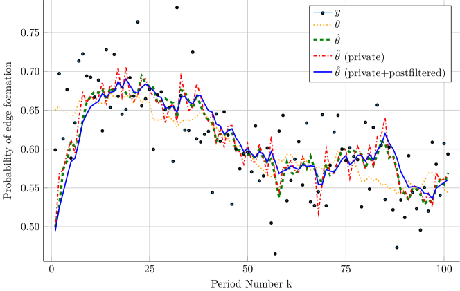
Figure 2. Sample path of the estimate of the edge formation probability $\theta_{k}^{ab}$, for some classes $(a,b)$. The measured edge density is generated from one component of the model (5.1), (5.2) with $f=1$ and $w_{k},v_{k}$ iid Gaussian random variables with zero mean and standard deviation $0.03$ and $0.04$ respectively. The trajectory $\theta$ (dotted line) starts at the value $0.65$, and the observers are all initialized at the value $0.50$. The upper bound $\rho$ on the contraction rate of the observer (5.4) is set to $\rho=0.9$, providing a good tradeoff between convergence speed and steady-state variance (see green dashed curve for the non-private observer), with corresponding gain $h=1.11$. The dot-dashed line shows $1/(1+\exp(-\tilde{z}_{k}))$ as our private estimate of $\theta_{k}$, where $\tilde{z}_{k}$ is a $\ln(3)$-differentially private estimate of $\psi_{k}$ (hence, the estimate of $\theta_{k}$ is also $\ln(3)$-differentially private), obtained by the Laplace mechanism, for the adjacency relation (2.6) with parameter values $K=3\times 10^{-3}$, $\alpha=0.25$. We also show a differentially private estimate obtained after further post-filtering, as explained in the main text.

5.2. Syndromic Surveillance

Syndromic surveillance systems monitor health related data in real-time in a population to facilitate early detection of epidemic outbreaks [39]. In particular, recent studies have shown the correlation between certain non-medical data, e.g., search engine queries related to a specific disease, and the proportion of individuals infected by this disease in the population [40]. Although time series analysis can be used to detect abnormal patterns in the collected data [39], here we focus on a model-based filtering approach [41], and develop a differentially private observer for a $2$-dimensional epidemiological model.

The following SIR model of Kermack and McKendrick [42, 43] models the evolution of an epidemic in a population by dividing individuals into 3 categories: susceptible (S), i.e., individuals who might become infected if exposed; infectious (I), i.e., currently infected individuals who can transmit the infection; and recovered (R) individuals, who are immune to the infection. A simple version of the model in continuous-time includes bilinear terms and reads

$$\frac{ds}{dt} =-\mu\mathcal{R}_{o}is$$

$$\frac{di}{dt} =\mu\mathcal{R}_{o}is-\mu i.$$

Here $i$ and $s$ represent the proportion of the total population in the classes $I$ and $S$. The last class $R$ need not be included in this model because we have the constraint $i+s+r=1$. The parameter $\mathcal{R}_{o}$ is called the basic reproduction number and represents the average number of individuals infected by a sick person. The epidemic can propagate when $\mathcal{R}_{o}>1$. The parameter $\mu$ represents the rate at which infectious people recover and move to the class $R$. More details about this model can be found in [43].

Discretizing this model with sampling period $\tau$, we get the discrete-time model

(5.8) $$s_{k+1} =s_{k}-\tau\mu\mathcal{R}_{o}i_{k}s_{k}+w_{1,k}=f_{1}(s_{k},i_{k})+w_{1,k}$$

(5.9) $$i_{k+1} =i_{k}+\tau\mu i_{k}(\mathcal{R}_{o}s_{k}-1)+w_{2,k}=f_{2}(s_{k},i_{k})+w_{2,k},$$

where we have also introduced noise signals $w_{1}$ and $w_{2}$ in the dynamics. We assume here for simplicity that we can collect syndromic data providing a noisy measurement of the proportion of infected individuals, .i.e.,

$$y_{k}=i_{k}+v_{k},$$

where $v_{k}$ is a noise signal. We can then consider the design of an observer of the form

$$\hat{s}_{k+1} =f_{1}(\hat{s}_{k},\hat{i}_{k})+h_{1}(y_{k}-\hat{i}_{k})$$

$$\hat{i}_{k+1} =f_{2}(\hat{s}_{k},\hat{i}_{k})+h_{2}(y_{k}-\hat{i}_{k}).$$

We define the Jacobian matrix of the system (5.8), (5.9)

$$F(s,i)=I_{2}+\tau\mu\mathcal{R}_{o}\begin{bmatrix}-i&-s\\ i&s-1/\mathcal{R}_{o}\end{bmatrix},$$

as well as the gain matrix $H=[h_{1},h_{2}]^{T}$ and observation matrix $C=[0,1]$. Here, we design a differentially private observer with Gaussian noise using Corollolary 8, for the adjacency relation (2.6) with $p=2$.

Following Corollary 3, the contraction rate constraint (4.7) for a 2-norm on $\mathbb{R}^{2}$ weighted by a matrix $P\succ 0$ is equivalent to the family of inequalities, for all $(s,i)$ in the region of $[0,1]^{2}$ where we want to show contraction

$$(F(s,i)-HC)^{T}P(F(s,i)-HC)\preceq\rho^{2}P$$

$$F_{x}^{T}PF_{x}-F_{x}^{T}PHC-C^{T}H^{T}PF_{x}+C^{T}H^{T}PHC\preceq\rho^{2}P,$$

where we used $F_{x}:=F(s,i)$ to simplify the notation. Defining the new variable $X=PH$, this can be rewritten

$$F_{x}^{T}PF_{x}-F_{x}^{T}XC-C^{T}X^{T}F_{x}+C^{T}X^{T}P^{-1}XC\preceq\rho^{2}P,$$

which, using the Schur complement, is equivalent to the family of LMIs

(5.10) $$\begin{bmatrix}\rho^{2}P-F_{x}^{T}PF_{x}+F_{x}^{T}XC+C^{T}X^{T}F_{x}&C^{T}X^{T}\\ XC&P\end{bmatrix}\succeq 0,$$

for all $x=(s,i)$ in the region where we want to prove contraction. If we can find $P,X$ satisfying these inequalities, we recover the observer gain vector simply as $H=P^{-1}X$.

For a given value of $\rho$, the covariance matrix of the Gaussian noise in Corollary 8 is proportional to $\|P^{1/2}H\|_{2}^{2}P^{-1}=(H^{T}PH)P^{-1}=(X^{T}P^{-1}X)P^{-1}$, and hence it is advantageous to minimize a function of this matrix. Note that $X^{T}P^{-1}X$ is a scalar. Minimizing $(X^{T}P^{-1}X)\,\text{Tr}(P^{-1})$ does not appear to directly lead to an efficiently solvable optimization problem, but as a proxy we can choose to minimize instead the sum $X^{T}P^{-1}X+\nu\text{Tr}(P^{-1})$, for some tuning parameter $\nu$. After taking Schur complements, this leads to the following semidefinite program, for a given value of the contraction parameter $\rho$

$$\min_{\Sigma\succeq 0,\lambda\geq 0,P\succeq 0,X}\quad \lambda+\nu\,\text{Tr}(\Sigma)$$

subject to $$\begin{bmatrix}\lambda&X^{T}\\ X&P\end{bmatrix}\succeq 0,\;\;\begin{bmatrix}\Sigma&I_{2}\\ I_{2}&P\end{bmatrix}\succeq 0,\text{ and }\eqref{eq: LMI contraction rate}.$$

Alternatively, one can minimize $\lambda\text{Tr}(\Sigma)$ for fixed values of $\lambda$ subject to the constraints above and perform a one-dimensional search for a minimizing value of $\lambda$.

Example 2.

Let us assume $\mu=0.1$, $\mathcal{R}_{o}=2$, $\tau=0.1$, $K=10^{-3},\alpha=0.25$ in (2.6), and $\epsilon=2$, $\delta=0.05$. That is, we wish to provide a $(2,0.05)$-differential privacy guarantee for maximum deviations of $0.1\%$ (see the discussion in the previous subsection). Although not a perfectly rigorous contraction certificate, we sample the continuous set of constraints (5.10) by sampling the set $\{(s,i)|0.01\leq i\leq 0.25,0.01\leq s\leq 1-i\}$ at the values of $s,i$ multiple of $0.01$, to obtain a finite number of LMIs. A more rigorous approach to enforce these constraints could make use of sum-of-squares programming [44]. Following the procedure above, for the choice $\rho=0.996$, we obtain the observer gain $H=[3.9304;0.2003]$ and the covariance matrix $\Sigma$ with $\Sigma^{1/2}=\begin{bmatrix}691&22\\ 22&17\end{bmatrix}\times 10^{-4}$ for the privacy-preserving Gaussian noise. Sample trajectories of the non-private and private (non-smoothed) estimates of $i$ are shown on Fig. 3.

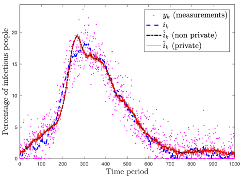
Figure 3. Sample path of the estimate of the percentage of infectious people over time produced by the observer. The standard deviations for the dynamics and measurement noise were set to $\sigma_{w_{k}}I_{2}=0.005\sqrt{\tau}I_{2}$ and $\sigma_{v_{k}}=0.02$ respectively. The signals were truncated to maintain positive values for $i,s,y$ in the simulation. The true proportion of infectious people starts at $0.5\%$, whereas the estimate used to initialize the observer is $1\%$. The output of the differentially private observer is not filtered.

6. Conclusion

This paper introduces a design methodology for nonlinear observer design, which provides differential privacy guarantees when the measured signals are privacy sensitive, by perturbing the published output signal of the observer. Tools from contraction analysis are used both to enforce convergence of the observer and to set the level of output noise necessary in order to provide the differential privacy guarantee. More concretely, we bound the sensitivity of the observers by leveraging a robustness property of contractive systems. The observer design methodology is illustrated through two examples where we construct estimators for models with nonlinear dynamics or measurements.

References

- [1] J. Le Ny, “Privacy-preserving nonlinear observer design using contraction analysis,” Proceedings of the 54th Conference on Decision and Control (CDC), (Osaka, Japan), pp. 4499–4504, December 2015. DOI: 10.1109/CDC.2015.7402922.
- [2] S. D. Warren and L. D. Brandeis, “The right to privacy,” Harvard Law Review, vol. 4, pp. 193–220, December 1890. DOI: 10.2307/1321160.
- [3] P. McDaniel and S. McLaughlin, “Security and privacy challenges in the smart grid,” IEEE Security Privacy, vol. 7, no. 3, pp. 75–77, 2009.
- [4] President’s Council of Advisors on Science and Technology, “Big data and privacy: A technological perspective,” Tech. Rep. Report to the President, Executive Office of the President of the United States, May 2014.
- [5] “Tracking and hacking: Security and privacy gaps put american drivers at risk,” Tech. Rep. U.S. Senator’s report, Staff of Senator E. J. Markey, February 2015.
- [6] A. Narayanan and V. Shmatikov, “Robust de-anonymization of large sparse datasets (how to break anonymity of the Netflix Prize dataset),” Proceedings of the IEEE Symposium on Security and Privacy, (Oakland, CA), May 2008.
- [7] J. A. Calandrino, A. Kilzer, A. Narayanan, E. W. Felten, and V. Shmatikov, ““You might also like”: Privacy risks of collaborative filtering,” Proceedings of the IEEE Symposium on Security and Privacy, (Berkeley, CA), May 2011.
- [8] D. H. Wilson and C. Atkeson, “Simultaneous tracking and activity recognition (STAR) using many anonymous, binary sensors,” in Pervasive Computing (H.-W. Gellersen, R. Want, and A. Schmidt, eds.), vol. 3468 of Lecture Notes in Computer Science, pp. 62–79, Springer, 2005.
- [9] L. Sankar, W. Trappe, K. Ramchandran, H. V. Poor, and M. Debbah, eds., IEEE Signal Processing Magazine, Special issue on Signal Processing for Cybersecurity and Privacy., September 2013.
- [10] C. Dwork, F. McSherry, K. Nissim, and A. Smith, “Calibrating noise to sensitivity in private data analysis,” Proceedings of the Third Theory of Cryptography Conference, (New York, NY), pp. 265–284, March 2006.
- [11] C. Dwork, M. Naor, T. Pitassi, and G. N. Rothblum, “Differential privacy under continual observations,” Proceedings of the ACM Symposium on the Theory of Computing (STOC), (Cambridge, MA), June 2010.
- [12] T.-H. H. Chan, E. Shi, and D. Song, “Private and continual release of statistics,” ACM Transactions on Information and System Security, vol. 14, pp. 26:1–26:24, November 2011.
- [13] J. Le Ny and G. J. Pappas, “Differentially private Kalman filtering,” Proceedings of the 50th Annual Allerton Conference on Communication, Control, and Computing, October 2012.
- [14] J. Bolot, N. Fawaz, S. Muthukrishnan, A. Nikolov, and N. Taft, “Private decayed predicate sums on streams,” Proceedings of the 16th International Conference on Database Theory, (Genoa, Italy), pp. 284–295, March 2013.
- [15] J. Le Ny and G. J. Pappas, “Differentially private filtering,” IEEE Transactions on Automatic Control, vol. 59, pp. 341–354, February 2014.
- [16] J. Le Ny and M. Mohammady, “Differentially private MIMO filtering for event streams,” IEEE Transactions on Automatic Control, vol. 63, January 2018.
- [17] A. McGlinchey and O. Mason, “Differential privacy and the sensitivity of positive linear observers,” Proceedings of the 20th IFAC World Congress, (Toulouse, France), pp. 3111–3116, July 2017.
- [18] W. Lohmiller and J.-J. Slotine, “On contraction analysis for non-linear systems,” Automatica, vol. 34, no. 6, pp. 683–696, 1998.
- [19] E. D. Sontag, “Contractive systems with inputs,” in Perspectives in Mathematical System Theory, Control, and Signal Processing (J. Willems, S. Hara, Y. Ohta, and H. Fujioka, eds.), pp. 217–228, Springer-Verlag, 2010.
- [20] F. Forni and R. Sepulchre, “A differential Lyapunov framework for contraction analysis,” IEEE Transactions on Automatic Control, vol. 59, pp. 614–628, March 2014.
- [21] D. Angeli, “A Lyapunov approach to incremental stability properties,” IEEE Transactions on Automatic Control, vol. 47, pp. 410–421, March 2000.
- [22] E. D. Sontag and Y. Wang, “Output-to-state stability and detectability of nonlinear systems,” Systems and Control Letters, vol. 29, pp. 279–290, February 1997.
- [23] J.-P. Gauthier and I. Kupka, Deterministic Observation Theory and Applications. Cambridge University Press, 2001.
- [24] A. Isidori, Lectures in Feedback Design for Multivariable Systems. Springer, 2017.
- [25] J. Cortés, G. E. Dullerud, S. Han, J. Le Ny, S. Mitra, and G. J. Pappas, “Differential privacy in control and network systems,” Proceedings of the 55th Conference on Decision and Control, (Las Vegas, NV), December 2016.
- [26] S.-J. Chung, S. Bandyopadhyay, I. Chang, and F. Y. Hadaegh, “Phase synchronization control of complex networks of lagrangian systems on adaptive digraphs,” Automatica, vol. 49, pp. 1148–1161, May 2008.
- [27] H. K. Khalil, Nonlinear Systems. Prentice Hall, 2002.
- [28] D. C. Lewis, “Metric properties of differential equations,” American Journal of Mathematics, vol. 71, pp. 294–312, April 1949.
- [29] P. Hartman, Ordinary Differential Equations, 2nd Ed. Birkhäuser, 1982.
- [30] N. Aghannan and P. Rouchon, “An intrinsic observer for a class of Lagrangian systems,” IEEE Transactions on Automatic Control, vol. 48, pp. 936–945, June 2003.
- [31] A. Pavloc, N. van de Vouw, and H. Nijmeijer, Uniform Output Regulation of Nonlinear Systems: A Convergent Dynamics Approach. Birkhäuser, 2006.
- [32] G. Russo, M. di Bernardo, and E. D. Sontag, “Global entrainment of transcriptional systems to periodic inputs,” PLOS Computational Biology, vol. 6, no. 4, 2010.
- [33] M. P. do Carmo, Riemannian Geometry. Birkhäuser, 1992.
- [34] M. Vidyasagar, Nonlinear Systems Analysis. Prentice Hall, 2nd ed., 1993.
- [35] V. Lakshmikantham and D. Trigiante, Theory of Difference Equations: Numerical Methods and Applications. Prentice Hall, 2002.
- [36] K. S. Xu and A. S. Hero III, “Dynamic stochastic blockmodels for time-evolving social networks,” Journal of Selected Topics in Signal Processing, vol. 8, pp. 552–562, August 2014. Special Issue on Signal Processing for Social Networks.
- [37] P. W. Holland, K. B. Laskey, and S. Leinhardt, “Stochastic blockmodels: first steps,” Social Networks, vol. 5, no. 2, pp. 109–137, 1983.
- [38] L. Wasserman and S. Zhou, “A statistical framework for differential privacy,” Journal of the American Statistical Association, vol. 105, pp. 375–389, May 2010.
- [39] A. B. Lawson and K. Kleinman, Spatial and Syndromic Surveillance for Public Health. Wiley, 2005.
- [40] J. Ginsberg, M. H. Mohebbi, R. S. Patel, L. Brammer, M. S. Smolinski, and L. Brilliant, “Detecting influenza epidemics using search engine query data,” Nature, vol. 457, pp. 1012–1014, 2009.
- [41] A. Skvortsov and B. Ristic, “Monitoring and prediction of an epidemic outbreak using syndromic observations,” Mathematical biosciences, vol. 240, pp. 12–19, 2012.
- [42] W. O. Kermack and A. G. McKendrick, “A contribution to the mathematical theory of epidemics,” Proceedings of the Royal Society of London Series A, vol. 115, pp. 700–721, 1927.
- [43] F. Brauer, P. van den Driessche, and J. Wu, Mathematical Epidemiology. Lecture Notes in Mathematics, vol. 1945, Springer-Verlag, 2008.
- [44] E. M. Aylward, P. A. Parrilo, and J.-J. E. Slotine, “Stability and robustness analysis of nonlinear systems via contraction metrics and SOS programming,” Automatica, vol. 44, pp. 2163–2170, August 2008.