The multilayer shallow water system in the limit of small density contrast
Abstract
We study the inviscid multilayer Saint-Venant (or shallow-water) system in the limit of small density contrast. We show that, under reasonable hyperbolicity conditions on the flow and a smallness assumption on the initial surface deformation, the system is well-posed on a large time interval, despite the singular limit. By studying the asymptotic limit, we provide a rigorous justification of the widely used rigid-lid and Boussinesq approximations for multilayered shallow water flows. The asymptotic behaviour is similar to that of the incompressible limit for Euler equations, in the sense that there exists a small initial layer in time for ill-prepared initial data, accounting for rapidly propagating “acoustic” waves (here, the so-called barotropic mode) which interact only weakly with the “incompressible” component (here, baroclinic).
1 Introduction
1.1 Presentation of the models and the problem
This work dedicated to the study of the so-called multilayer Saint-Venant system, which arises as an approximate model for the propagation of waves in the ocean or atmosphere, when density stratification cannot be neglected. We will refer to as free surface system the following first-order, quasilinear system of coupled evolution equations:
| (1.1) |
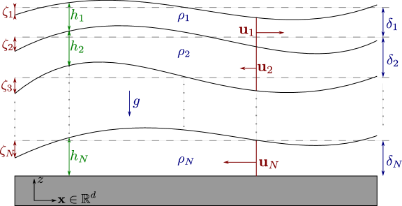
Here, the unknowns and represent respectively the deformation of the interface and the layer-averaged horizontal velocity in the layer, at time and horizontal position where ; see Figure 1. If , then we denote and . We denote by the mass density of the homogeneous fluid in the layer, whereas is the gravitational acceleration. Finally,
is the depth of the layer. By convention, we set (above the upper free surface is vacuum), and (the bottom is flat). We restrict ourselves to the setting of stable stratification, namely
We may rescale the variables so as to replace the factor
More precisely, we use the following nondimensionalization:
where is a characteristic horizontal length (say the wavelength of the flow), is a characteristic vertical length (say the typical depth of one layer at rest), and is a velocity. 111Because we assume that the layers are all of comparable depth and the vertical stratification is balanced, in the sense that we fix such that , then measures the typical velocity of propagation of the baroclinic modes; see Appendix B.
Although does not appear in our system, it plays a very important role as the Saint-Venant system may be seen as the first-order asymptotic model obtained from the full multilayer water-wave system in the limit ; see [25, 11] in the one-layer case and [15] in the bilayer (albeit irrotational) setting. It may also be formally obtained using the hydrostatic and columnar motion assumptions; see [38, 34, 5, 26, 39].
In this work, we ask
Qn: What is the behaviour of the solutions to (1.1) in the limit ?
The first observation is that the velocity evolution equations become singular, as since by convention, so that even the existence of solutions on a non-trivial time interval is far from straightforward.
At the linear level, it is known [40] (see also Appendix B) that the flow may be decomposed into modes, propagating as linear wave equations with distinct velocities. In our setting, the first mode, i.e. the barotropic mode, propagates much faster than the other, baroclinic modes, in the sense that the former is typically of size while the latter are uniformly bounded when ; hence the singularity. While such a decomposition is exact only in the linear setting, we show in this work that the flow behaves in a similar way in the weak density contrast limit even when strong nonlinearities are present, provided that the initial surface deformation is small, the depth of each layer remains positive and shear velocities are not too large. Roughly speaking, we show that one may then approximate the flow as the superposition of rapidly propagating acoustic waves and a non-singular “slow” mode with non-trivial dynamics.
Let us be more precise. Asymptotically, the fast mode describes the propagation of the free surface, , and total volume flux, namely where and is the orthogonal projection onto irrotational vector fields. One has at first order, in dimension and provided that and are initially balanced so that , the linear acoustic system
| (1.2) |
The slow component contains all the baroclinic modes which interact strongly one with each other in the nonlinear setting. We show that it is asymptotically described by the rigid-lid model, which is obtained from the free-surface system by setting in the mass conservation equations, and replacing with in the velocity evolution equations (see [27, 5]). In addition, we apply the so-called Boussinesq approximation (see e.g. [20]) to the limit system, that is we set in the velocity evolution equations while remains fixed and non-trivial. This yields
| (1.3) |
with the same notation as before, except and . In particular, the first equation is not an evolution equation but a constraint (conservation of total mass), namely
Physically speaking, is (up to a constant) the pressure at the flat, rigid lid. From a mathematical viewpoint, is the Lagrange multiplier associated with the above divergence-free constraint. It may be reconstructed from the knowledge of by solving the Poisson equation
We thus offer a rigorous justification (the formal justification is generally attributed to Armi [2]) of the widely used rigid-lid and Boussinesq approximations for free surface multilayer shallow-water flows with a small density contrast.
1.2 Main results
Before stating our main results, let us recall for convenience the system of equations at stake:
| (1.4) |
where with convention and . In the following, we fix parameters ; and denote
We can then reconstruct with () and where is the only parameter allowed to vary, and by assumption
It is also convenient to denote (notice the prefactor; see Remark 1.3 below)
so that the control of in Sobolev space (see Appendix A for notations) yields, when ,
Let us now state the main results of this work.
Theorem 1.1 (Large time well-posedness).
Let and be such that
| (1.5) |
where , and we recall the convention .
Theorem 1.2 (Strong convergence).
Let , , and as above. Then there exists with and, for sufficiently small,
-
•
a unique strong solution to (1.4) and ;
-
•
a unique strong solution to (1.3) with initial data
where is the total depth, with convention and the orthogonal projection onto irrotational vector fields.
-
•
a unique strong solution to (1.2) with
Moreover, one has for any ,
where .
Remark 1.3.
As mentioned in the introduction, our hypotheses contain a smallness assumption on the initial deformation of the surface, namely . This assumptions is natural so as to balance the contributions in the (preserved in time) energy:
Without this assumption, the flow possesses a strongly nonlinear barotropic component, and energy methods yield a well-posedness theory over a small time-domain, , ; see Proposition 2.1 and Remark 2.2, below. On this timescale, the baroclinic component do not evolve, so that all the dynamics is described by the barotropic component (asymptotically as ).
Remark 1.4.
Remark 1.5.
Our proof does not rely on, but rather provides, the existence and uniqueness of strong solutions of the limit (rigid-lid) system. In that respect, one may see the free-surface system (1.4) as a penalized model for (1.3) relaxing the rigid-lid constraint. Sharper well-posedness results for the rigid-lid system in the two-layer case and without the Boussinesq approximation are provided in [21, 8].
Remark 1.6.
Theorem 1.2 is restricted to because we use dispersive decay estimates on rapidly propagating acoustic waves in order to control nonlinear coupling effects between the fast and slow modes. In the case of dimension , and provided that the initial data is sufficiently localized in space, we justified in [16] a similar mode decomposition of the flow, by making use of the different spatial support of each mode after small time. Proposition 4.4 therein, together with Proposition 3.8 in the present work, offer a convergence between the exact and the approximate solution with rate . The same convergence rate holds in the case of dimension and well-prepared initial data, in the sense of Proposition 4.2.
In the following, for the sake of simplicity, we limit our study to the case of dimension , although we find it more telling to keep the notation . The proof of Theorem 1.1 is easily adapted to the case of dimension .
Remark 1.7.
One could add, without any additional difficulty, a uniformly bounded and order-zero term to the system, so as to take into account for instance the Coriolis force, atmospheric pressure variations, or bottom topography. Notice however that these terms should be of size in the evolution equation for ; in particular, only small topography may be dealt with using directly our strategy. Similarly, except in the one-layer case where the the component due to Coriolis effect is an anti-symmetric perturbation of a symmetric system, one cannot allow a rapid rotation such as in the quasi-geostrophic regime, which would correspond here to where is the Rossby number; see [17, 36].
Remark 1.8.
Our results are valid for arbitrary , but not uniformly. In particular, we cannot control the dependence of as grows. Thus our strategy cannot be adapted to study the system in the limit , corresponding to the physically relevant situation of continuous stratification. A similar shortcoming was already noticed and discussed by Ripa in [37].
1.3 Discussion and strategy
A well-posedness result on system (1.4) is stated and proved in [31]. It follows from a standard analysis on quasilinear systems since a symbolic symmetrizer may be exhibited (see Section 2 below). However, due to the presence of singular components in the system, the a priori maximal time of existence of the solutions may be bounded from below only as using this method. Such a result is unsuitable for our purpose as the time interval shrinks to zero in the considered limit, and is inconsistent with oceanographic observations of large amplitude internal waves propagating over long distances; see e.g. [33] and references therein.
In order to go beyond this analysis and provide a time of existence of solutions uniformly bounded from below with respect to small, we need to take advantage of some additional structural properties of the system. This structure is put to light by a suitable change of variable, which we describe below.
Let us introduce the shear velocities, , and the total horizontal momentum, , as follows:
| (1.7) |
so that, conversely, for any ,
| (1.8) |
One may rewrite system (1.4) using the new variables as follows:
| (1.9) |
where , and are meant as the expressions in terms of given in (1.8).
The above change of variables may be seen as an approximate normal form allowing to decouple the slow and fast components of the flow. Indeed, since
one sees immediately that the singular terms appear only as linear components on the evolution equations for and —or more precisely — and involve only and . In other words, the leading-order terms form a system of rapidly propagating acoustic waves in :
The remainder contains quasilinear components depending on both the fast () and slow () variables, so we need to consider the full system of equations (1.9) in order to obtain the desired uniform energy estimates.
Let us now, for the sake of simplicity, restrict our discussion to the case of dimension . From the above, we may rewrite the system (1.9) as
| (1.10) |
where , so that represents the above acoustic wave system for the fast variables, while ; and contains lower-order (in terms of ) and coupling terms.
We shall make use of the fact that one can construct a “good” symmetrizer of the system under the form (1.10), namely we exhibit real, positive-definite matrices such that and , and satisfying the decomposition
where is the orthogonal projection onto , the slow variables. Indeed, one obtains an energy estimate by taking the inner-product of the equation with , which only requires to estimate
Using that and are constant operators and that , we see that the above are estimated uniformly with respect to small; thus we have a uniform control of the norm. The corresponding estimate with does not bring additional difficulties, using that commutes with the Fourier multiplier .
There remains to understand why such symmetrizer exists for our system (1.10). One could check, after tedious calculations, that the explicit one provided by Monjarret in [31] (after applying the congruent transformation associated with the change of variables) satisfies the necessary hypotheses, but we offer in Appendix B an alternative and more robust construction. We show that, provided that satisfies (1.5),(1.6), then has real and distinct eigenvalues. Two of them are asymptotically equivalent to as while the other ones are uniformly bounded with respect to small. The spectral projection corresponding to the former converge towards the projections onto the eigenspaces corresponding the two non-trivial eigenvalues of . Using the scale separation between the eigenvalues, one shows that the spectral projections corresponding to the latter are uniformly bounded, and that they converge as towards independent, rank-one projections onto subspaces of . Our symmetrizer is then, classically,
where is the spectral projection onto the eigenspace of . That enjoys the desired properties follows, using standard perturbation theory [22], from the fact that is constant, and the strong scale separation between and uniformly bounded eigenvalues.
An additional difficulty arises in the situation of horizontal dimension , due to the fact that the symmetrizer of the system —which is constructed from the symmetrizer in dimension and a rotational invariance property— is only a symbolic symmetrizer, as opposed to symmetrizers in the sense of Friedrichs. Thus we rely on para-differential calculus, but extra care must be given to “lower order terms” in the sense of regularity, which may effectively hurt our energy estimates if they are not uniformly bounded with respect to . As a matter of fact, we use that one can construct an explicit operator (defined as a Fourier multiplier) which symmetrizes the linear, singular contributions of the system, and use para-differential calculus only on the next order components in terms of .
Given the uniform (with respect to small) energy estimates, the large time well-posedness (Theorem 1.1) follows from the standard theory for quasilinear hyperbolic systems. The convergence results (Theorem 1.2 as well as additional assertions in Section 5) proceed from rather standard techniques in the study of singular systems; see references below.
1.4 Related earlier results
In [16], the author studied the so-called inviscid bilayer Saint-Venant (or shallow water) system in the limit of small density contrast. The change of variables allowing for uniform energy estimates was exhibited therein, and convergence towards a solution of the rigid-lid limit, as well as a second-order approximation, was deduced in the case of well-prepared initial data. This work is therefore an extension of these results to the situation of (horizontal) dimension , ill-prepared initial data as well as arbitrary number of layers.
As already noticed in the aforementioned work, our problem has many similarities with the (two-dimensional) incompressible limit for Euler equations, as studied initially in [23, 24, 9]. As a matter of fact, if we consider only one layer of fluid, then our problem corresponds exactly to a special case of the isentropic incompressible limit, and we recover the results of Ukai [42] and Asano [3]. We will not detail the very rich history of results concerning this problem (we let the reader to [19, 28, 1] for comprehensive reviews) but rather aim at pointing out similarities and differences of our situation.
Let us first recall the two-dimensional isentropic Euler equations for inviscid, barotropic fluids:
| (1.11) |
where is a given pressure law, is the density, the velocity, and the dimensionless Mach number. As claimed above, one recognizes exactly (1.9) in the one layer setting (), by setting , and identifying
Of course, the difficulty in our case is that, as one considers additional layers of fluids, these equations are coupled with additional equations on additional unknowns, so as to produce a full quasilinear system. Since these additional equations are non-singular with respect to the small parameter, it is tempting to compare our situation with the incompressible limit for the non-isentropic Euler equations, where (1.11) is coupled with an additional evolution equation for the entropy, :
and .
Our situation, however, is quite different. This can be seen from the fact that, contrarily to the non-isentropic Euler equations, the linearized system is balanced, in the sense that a small perturbation of the “slow” component of the reference state induces only a small deviation for the solution. In other words, using the notation of the above discussion, the symmetrizer of the non-isentropic Euler equations does not satisfy but only ; see discussion in [30]. This additional property in our situation allows in particular to straightforwardly deduce energy estimates from the corresponding energy estimate; and to obtain the strong convergence result of Theorem 1.2 simply from dispersive estimates on the “acoustic” component of the flow, as originally carried out by Ukai [42] and Asano [3] in the isentropic case.
In order to deal with this situation, Métivier and Schochet [30] (see also [7]) rely on the fact that their system enjoys a diagonal block structure and that the symmetrizer commutes exactly with the singular operator, denoted in the above discussion. Roughly speaking, this means that we may control the compressible and isentropic component of the flow independently of the acoustic component by simply projecting onto . Since such assumptions are only approximately satisfied in our situation, our system is rather related to the “-balanced” (and not “-diagonal”) systems studied by Klainerman and Majda [23], although we do not restrict ourselves to well-prepared initial data.
In this spirit, our proofs rely as little as possible on explicit calculations, thus we expect that the general strategy may be successfully applied to other situations and other frameworks, such as the ones presented in [35]. This is why we use mostly in the following the terminology of “fast vs slow” mode/component instead of “barotropic vs baroclinic” which is more relevant to our initial oceanographic motivation (see [20]); or “acoustic vs incompressible” associated with Euler equations.
1.5 Outline of the paper
In Section 2, we recall that our quasilinear system admits an explicit (symbolic) symmetrizer, which yields immediately a well-posedness theory for (1.4), for any fixed .
In Section 3.1, we exhibit the structural properties enjoyed by our system, after the change of variables (1.7),(1.8), and which allow the uniform (with respect to small) energy estimates provided in Section 3.2 (Proposition 3.5) and Section 3.3 (Proposition 3.8).
We deduce in Section 4 the large-time well-posedness result of Theorem 1.1. Additionally, we show in Proposition 4.2 that an assumption of well-prepared initial data is propagated by the flow for positive times.
Section 5 is dedicated to convergence results. We first state in Proposition 5.1 a weak convergence result for the solutions of the free-surface system as . As in the incompressible limit for Euler equations, the convergence cannot be strong uniformly in time, due to the rapidly propagating fast mode. However, we show in Proposition 5.2 that this small initial layer in time vanishes in the case of well-prepared initial data, and then characterize the defect for general initial data in Section 5.3, yielding Theorem 1.2.
Appendix A contains a description of some notations used throughout the text, as well as a short review of standard results concerning product and commutator estimates in Sobolev spaces (Section A.2) and Bony’s paradifferential calculus (Section A.3).
Finally, Appendix B is dedicated to some results on the eigenstructure of our system, which are used in Section 3.1.
2 Standard well-posedness theory
In this section, we fix and construct an explicit (symbolic) symmetrizer of (1.4). This offers a well-posedness result similar to Theorem 1.1, although non-uniformly with respect to small. This analysis has been provided by Monjarret in [31]; we recall it here for the sake of completeness and because the objects defined therein will be of later use.
Let us first rewrite the free-surface system (1.4) with a matricial, compact formulation. Provided that with , one can rewrite (1.4) equivalently as
| (2.1) |
with
| (2.2) |
Here and thereafter, we heavily make use of the block structure of -by- matrices. We denote by the -by- matrix with only zero entries, and for , . Moreover, are upper-triangular and is lower-triangular and are defined by
Proposition 2.1 ([31], Theorem 2.8).
Let and be such that
| (2.3) |
where we recall that by convention. One can set such that if satisfies additionally
| (2.4) |
then there exists a unique and , maximal solution to (2.1) and .
Remark 2.2.
Naively following the above strategy and keeping track of the dependency of constants with respect to the parameter would yield a disappointing lower bound on the maximal time of existence, namely , even when the initial surface deformation is assumed small as in Theorem 1.1. It is the main result of this work that, in this case, the well-posedness theory and uniform energy estimates can be extended to a non-shrinking time domain as .
The conditions (2.3),(2.4) ensure that the symmetrizer, defined in (2.7) below, is coercive. It is therefore a sufficient condition for hyperbolicity. Except in very specific cases, one has very few information on the domain of hyperbolicity; see discussion in Appendix B.
The fact that (2.4) requires a control on the shear velocities, rather than on the velocities themselves is allowed by some freedom in the choice of the symmetrizer. Notice in particular that the Hessian of the conserved energy yields a natural symmetrizer for our system of conservation laws in the case of irrotational flows, but it does not enjoy the desired property.
The ability to construct symmetrizers depending strongly on the shear velocities but only weakly on a background velocity (or on the total volume flux) is also essential for us to obtain results outside of the scope of well-prepared initial data; see [16] for an analysis where this property is not used.
Proof.
Let us introduce the symbol of (2.1):
An important property of our system is that is satisfies rotational invariance [31, Section 1.2]. More precisely, one can easily check that
| (2.5) |
where
| (2.6) |
where is the -by- identity matrix and . Obviously, is homogeneous of degree in , with entries in and is orthogonal: .
This allows to construct a (symbolic) symmetrizer of the system from a (Friedrichs) symmetrizer of alone. More precisely, define
| (2.7) |
with and where ,
and the parameter may be chosen freely in .
That is symmetric is easily checked once we notice the following identities in (2.1): , and .
It follows that is a symbolic symmetrizer of (2.1), since
is obviously symmetric. Finally, one may choose for instance, so that as soon as satisfies (2.3),(2.4) with sufficiently small, then is strictly diagonally dominant with positive diagonal entries, and therefore definite positive, uniformly for any .
3 Uniform energy estimates
In this section, we establish uniform (with respect to small) energy estimates, which are the essential ingredients in the proof of our main results. We first exhibit in Section 3.1 some properties of the system obtained after the change of variables (1.7)-(1.8), and which allow the energy estimate of Proposition 3.5 (Section 3.2) and in turn the energy estimate of Proposition 3.8 (Section 3.3).
3.1 A new formulation
In what follows, we fix and always assume that
| (3.1) |
(recall the convention: ). More precisely, we work with defined by
Consequently, the change of variables (1.7)-(1.8) define self-homeomorphisms between
and we denote
Consider the Jacobian matrix associated to :
| (3.2) |
where
From the inverse function theorem, one has
| (3.3) |
and
where (as is easier seen directly from (1.8)),
Applying the change of variables in (2.1) yields, for sufficiently regular functions (see Lemma 4.1 below),
| (3.4) |
which we can identify with (1.9), and where are explicitly given in terms of (displayed in (2.2)) and through
| (3.5) |
Finally, we denote by the orthogonal projection onto the “fast” variables, namely
| (3.6) |
with and .
The following result is now straightforward.
Lemma 3.1.
Let , and recall the definition of in (2.6). Then
| (3.7) |
Moreover, are well-defined and smooth and satisfy
| (3.8a) | |||
| (3.8b) | |||
| (3.8c) | |||
Proof.
Only the last estimate requires an explanation. Remark that the first variable of contributes to only through . Thanks to the prefactor, one deduces that
where we denoted . Similarly, by (1.7), one has
and, by definition, , so that
where represents the velocity variables of , as given by (1.8). The result is now clear. ∎
Lemma 3.2.
The functions are well-defined and smooth and satisfy the rotational invariance
| (3.9) |
as well as the following estimates:
| (3.10a) | |||
| (3.10b) | |||
Proof.
Estimates (3.10) may be deduced from identity (3.5) and the explicit expressions of and given in (2.2),(3.3),(3.2). They are also apparent when identifying (3.4) with (1.9). In particular, one immediately sees that the evolution equations for are non-singular (for small), and the singular term on the evolution equation for involves only , so that
and
The only singular terms (for small) arise from the first and last equations, which read
where are smooth and enjoy the same estimates as above. We now only need to remark that (by definition) and, since ,
where, again, is smooth and uniformly estimated as above. Lemma 3.2 is now straightforward. ∎
Finally, let us provide some estimates on the symbolic symmetrizer of the system.
Lemma 3.3.
There exists a smooth function such that
Moreover, one can set such that if and satisfy
| (3.11) |
then one has the following estimates:
| (3.12a) | |||
| (3.12b) | |||
| (3.12c) | |||
Proof.
One could define the symmetrizer as where is the symmetrizer associated with and has been displayed in (2.7), and check the properties directly on this explicit symmetrizer. Some of the estimates, however, rely on delicate cancellations which have no obvious explanation using this method. This is why we find it more instructive to construct our symmetrizer using the spectral properties of our system, whose study we postpone to Appendix B for the sake of readability. It is proved in Lemmas B.1 and B.3 that has only real and semisimple eigenvalues:
where , and are rank-one spectral projections. We now define
| (3.13) |
Indeed, is obviously symmetric, and so is
and one has for any ,
The upper bound in (3.12a) follows from
which is given by (3.8b) in Lemma 3.1 with (B.1) in Lemma B.1, and (B.2c) in Lemma B.2 with (B.3c)-(B.3e) in Lemma B.3. This proves (3.12a).
We conclude this section by collecting the above information on the symbols of our operators:
3.2 energy estimate
The following proposition shows that, thanks to the structure of the system exhibited in the previous section, one is able to control the () energy of solutions, uniformly on a time interval independent of small. This is the key ingredient in the proof of our main results.
Proposition 3.5.
This section is dedicated to the proof of this result. The main ingredients are the properties of the symbol of system (3.15) as well as its symmetrizer, collected in Corollary 3.4. Energy estimates for such symmetrizable systems can be obtained thanks to Bony’s paradifferential calculus associated with these symbols; see [29]. We shall however be cautious as paradifferential calculus typically provides estimates “up to lower order operators”: while this is sufficient for regularity aspects, this could induce order-zero but large (namely non uniformly bounded with respect to small) remainder terms, preventing the desired uniform energy control stated in (3.16).
This is why we decompose the symbols into a first order contribution which admits a natural quantization as a Fourier multiplier, whereas only second-order contributions will be paradifferentialized. Let us be more specific. Define
where is a smooth non-negative cut-off function ( for and for ); and let be the associated paradifferential operator (see Definition A.2). Similarly, define
and the associated paradifferential operator; and
| (3.17) |
where and will be determined later on.
We claim in Lemma 3.6, below, that the properties on given in Corollary 3.4 are sufficient to show that is a uniformly bounded and coercive operator, and show a precise estimate on its time derivative, . In Lemma 3.7, we then rewrite (3.15) as a symmetric, paradifferential equation, from which the energy estimate (3.16) is easily deduced.
Lemma 3.6.
Proof.
That is self-adjoint is obvious (recall in particular that is orthogonal). Let us now decompose
where is obtained from by setting to zero all entries with , and (notice )
Using (3.14b) in Corollary 3.4, we can define such that
By (3.14e) in Corollary 3.4 and since satisfies (3.11), one has for any ,
Similarly, the Lipschitz estimate (3.14e) yields for any and ,
so that the contribution from is estimated thanks to Proposition A.3 (item i) as follows:
Similarly, using (3.14f) in Corollary 3.4 yields, uniformly in ,
and one obtains identically the corresponding estimates for derivatives with respect to . Thus Propositions A.3 and A.4 yield for any ,
One easily checks that the last contribution satisfies the same estimate:
Here, we used that for scalar functions and , one has
| (3.20) |
where is a universal constant (by duality, since for any , one has and ).
Thanks to the above estimates, one may choose sufficiently large so that one has
It is now clear (using that is orthogonal for ) that one can restrict as in the statement so that (3.18) holds.
As for the second part of the statement, by definition of the quantization (see Definition A.2) and since commutes with constant operators and Fourier multipliers, one has
Moreover, using (3.14e) in Corollary 3.4, one has
Again, one easily obtains the corresponding estimates for derivatives with respect to and Proposition A.3 (item i) yields
Estimate (3.19) is proved, and the proof of Lemma 3.6 is complete. ∎
Lemma 3.7.
Proof.
Notice first that, using the rotational invariance property (3.9), one has
Thus applying the operator to (3.15) yields (3.21) with
| (3.22) |
We first note that, using estimate (3.14a) in Corollary 3.4 yields immediately
We then deduce from estimate (3.14c) in Corollary 3.4 that
and in turn, by (3.20),
Thus there only remains to estimate
where
These terms are estimated exactly as in the proof of Lemma 3.6, i.e. using the paradifferential calculus of Propositions A.3 and A.4 together with the estimates of Corollary 3.4, thus we do not detail. Let us just indicate why these contributions are uniformly bounded with respect to small. The case of is quickly settled by (3.14c) in Corollary 3.4. As for , we decompose as above
The contribution from the second component is uniformly bounded with respect to small, again thanks to (3.14c) in Corollary 3.4. The contribution from the first component may also be uniformly bounded by remarking that
where we used (3.14a), (3.14e) and (3.14f) in Corollary 3.4.
Completion of the proof.
Assume is sufficiently regular, say , so that all the calculations below are well-defined. We compute the inner-product of identity (3.21) with : it follows
The second term on the right-hand-side is identically zero since is symmetric. The other terms are estimated thanks to Cauchy-Schwarz inequality and Lemmata 3.6 and 3.7. Altogether, this shows that provided we restrict and as in Lemma 3.6, one has
| (3.23) |
with . Estimate (3.16) follows from Gronwall’s Lemma and the coercivity of , i.e. (3.18) in Lemma 3.6, together with the control of provided in Lemma 3.7. The fact that the same estimate holds for general solution to (3.15) may be obtained by density and thanks to a standard regularization process; see [29, Theorem 7.1.11]. Proposition 3.5 is proved.
3.3 energy estimate
The energy estimate derived in Proposition 3.5 quickly induces a similar estimate, for any , by using once more the specific structure of our system of equations, namely that singular terms appear only as linear components of the system (3.4).
Proposition 3.8.
Proof.
Denote , with . Then one has
| (3.25) |
We shall apply Proposition 3.5 to the above system, thanks to the standard tools on Sobolev spaces recalled in Section A.2. Notice first that since since , Sobolev embedding yields
so that we only need to estimate the commutator on the right-hand-side of (3.25) to apply Proposition 3.5. Since commutes with , one has
Now, thanks to the product and commutator estimates recalled in Section A.2, and following the proof of Lemma 3.2, one easily checks that, for any ,
Obviously, since (by (3.9) ), one has
One could apply the estimate of Proposition 3.5 to satisfying (3.25), but one obtains a slightly stronger result by stepping back and using directly the differential inequality of the proof, namely (3.23):
with , and
where , and .
Estimate (3.24) follows from Gronwall’s Lemma and the coercivity of , i.e. (3.18) in Lemma 3.6. Again, this estimate is proved for sufficiently regular , but may be extended to general solution to (3.25) by density and thanks to a standard regularization process. This concludes the proof of Proposition 3.8. ∎
4 Well-posedness and stability estimates
In this section, we collect the information gathered in the previous sections, which quickly yield Theorem 1.1, as well as the propagation of well-prepared initial data (see Proposition 4.2).
Let us first recall that Proposition 2.1 offers the existence and uniqueness of a (maximal) solution to (1.4), for sufficiently regular initial data. Our results give additional information on the large time behaviour of these solutions, using in particular the energy estimates of Proposition 3.5 and 3.8. These estimates, however, are based on a different formulation of the equations, namely (1.9), which we claimed to be equivalent. Let us precisely state below in which sense.
Lemma 4.1.
Let with , satisfying (3.1). Then , defined by (1.7), satisfies and
Conversely, if satisfies (3.1), then the change of variables (1.8) defines and
Moreover, if as above is a strong solution to (2.1) (or, equivalently, (1.4)), then is a strong solution to (3.4) (or, equivalently, (1.9)); and conversely.
Proof.
Notice that implies immediately since is an algebra for any . The converse is also true since the multiplication by is continuous from to ; see Section A.2. It follows, by continuous Sobolev embedding, that all the terms in (1.4) and (1.9) as well as in the calculations below are well-defined in .
The evolution equations for in (1.9) are straightforwardly deduced from the ones for in (1.4). The evolution equation for follows from
Plugging the expression for in (1.4), and using , yields immediately the desired expression of the evolution equation for in (1.9).
The corresponding result concerning the compact matricial formulation of the systems, and in particular (3.5), is obvious by the chain rule.
This proves the first part of the statement. The second part is identical since all these calculations are reversible: the Jacobian associated to the change of variables is invertible; see (3.3). ∎
4.1 Large time well-posedness; proof of Theorem 1.1
By Proposition 2.1, one can set such that if (1.6) holds with , then there exists a unique strong solution to (2.1) and . By Lemma 4.1, the change of variable (1.7) defines and satisfies
and . Let us denote
We restrict our discussion below to , so that (by continuity) .
Using the system satisfied by , (3.14a) in Corollary 3.4 as well as Sobolev embeddings, one checks
for any ; recall is defined in (3.6).
In particular, one has for any ,
from which we deduce
and, similarly,
It follows that, for given , one can set such that if and (1.6) holds with , then satisfies the assumptions of Proposition 3.8 for any with
We thus deduce the energy estimate
with and . In particular this shows that one can choose such that
Going back to the original variables through (1.8) and by Lemma 4.1, this shows that one can restrict and the time interval , with bounded as above, so that is uniformly bounded and (2.3)-(2.4) remain satisfied. By continuity, uniqueness of the maximal solution and thanks to the blow-up criteria in Proposition 2.1, we deduce that one can set
This concludes the proof of Theorem 1.1.
4.2 Propagation of well-prepared initial data
Proposition 4.2.
Proof.
Let us denote by the solution to (1.4) and defined by Theorem 1.1; and by the associated solution to (3.4), namely
obtained through the change of variables (1.7) (see Lemma 4.1). Finally we denote . Using the above equation and the product estimates recalled in Section A.2, one has immediately .
Differentiating the above system of equations yields
By construction (see the proof of Theorem 1.1 above), one can restrict so that satisfies the assumptions of Proposition 3.5, namely (3.1)-(3.11) for ; and one has
| (4.1) |
By estimate (3.14a) in Corollary 3.4, one has
What is more, the additional smallness assumption on yields
uniformly for .
Altogether, after applying Proposition 3.5 with , one deduces
| (4.2) |
with . Applying Gronwall’s Lemma to yields
for sufficiently large.
5 Convergence results
In this section, we investigate the asymptotic behaviour of the previously obtained solutions in the limit . We first show that the solutions of the free-surface system (1.4) converge weakly towards solutions of the rigid-lid system (1.3). Strong convergence results are then obtained, first by assuming that the initial data is well-prepared, and then by approaching the oscillatory “defect” through rapidly propagating acoustic waves.
5.1 Weak convergence: the rigid-lid limit
Our first (weak) convergence result is the following.
Proposition 5.1.
As , let satisfying (1.5)-(1.6). Denote, for sufficiently small, the solution to (1.4) with . Then, as , converges weakly (in the sense of distributions and up to a subsequence) towards a solution of the rigid-lid system (1.3), with initial data
where , with convention and is the orthogonal projection onto irrotational vector fields.
Proof.
Restricting if necessary, satisfies the hypotheses of Theorem 1.1. Thus one can define from the solution to (1.4) with initial data ; and
with .
Thus, by Banach-Alaoglu theorem on , we can extract a weakly converging subsequence (in the sense of distributions), that we still denote :
with .
Let us first notice that since satisfies (1.4) one has, uniformly for ,
Thus, since the embedding of in is locally compact and by Aubin-Lions lemma and Cantor’s diagonal argument, one has (again up to the extraction of a subsequence) strongly in . It follows by the logarithmic convexity of Sobolev norms, that for any ,
Thereafter, we fix so that and is an algebra. For the same reasons as above, we have also
and, using ,
Let us now define
Notice now that all the (quadratic) nonlinear terms are strongly convergent, so that
and
with convention . Notice also that passing to the (weak) limit in the first equation of (1.4) yields
We now define
Notice the identity
so that
It follows, using the formula (1.8) with and , and since all the components converge strongly in , that converges strongly as well. By virtue of uniqueness of the weak limit, one has
We conclude by plugging the decomposition into the evolution equations for velocities in (1.4). Notice the identity, using that is irrotational,
Thus the only (quadratic) term which does not involve at least one strongly convergent factor turns out to be an exact gradient and independent of ; and so is the unbounded (linear) component of the equation, namely . This shows, passing to the weak limit all the other terms in the equation, that there exists , independent of , such that
It is straightforward to pass to the limit in the conservation of mass equations, so that
and we have already seen that .
5.2 Strong convergence for well-prepared initial data
Proposition 5.2.
Using the notations of Proposition 5.1, let as , with well-prepared as in Proposition 4.2. Then (up to extracting a subsequence) strongly in , for all , as .
Moreover, and , where is the pressure associated with solution to (1.3).
Proof.
We follow the proof of Proposition 5.1. However, we may use additionally that, thanks to Proposition 4.2 (and using the system of equations (1.4) to control time derivatives)
It follows (up to the extraction of a subsequence) and strongly in , and therefore in for ; and (in the sense of distributions).
By Banach-Alaoglu theorem, has a weak limit in when , and passing to the weak limit in the velocity evolution equations shows that this limit is . ∎
5.3 Strong convergence for ill-prepared initial data; proof of Theorem 1.2
The proof of Theorem 1.2 is divided in three parts. We first construct a “slow mode” approximate solution, thanks to the appropriate rigid-lid solution. We then construct a “fast mode” approximate solution, satisfying an acoustic wave equation with appropriate initial data. Finally, we show that, thanks to dispersive estimates on the fast mode, the coupling effects between the two modes are small, so that the superposition of the two components solves approximately the free-surface system (1.4) with appropriate initial data. The energy estimate of Proposition 3.5, applied to the difference between the exact and the approximate solution, allows to conclude.
Construction of the slow mode. Using Proposition 5.2 with well-prepared initial data
and artificially setting , one obtains in the limit
a solution to (1.3) with initial data
where we recall that is the total depth, with convention and the orthogonal projection onto irrotational vector fields. Moreover, the corresponding pressure satisfies , and one has
| (5.1) |
(since , the solutions of (1.4) with from which is constructed, satisfy the same estimate by Theorem 1.1).
Let us prove that one may (uniquely) choose . The regularity of strong solution to (1.3) is sufficient to claim that is uniquely defined by
where with convention . Notice now that
and
It follows, using that is an algebra, that there exists such that
Thus one may define a unique solution by Fourier analysis. 222Let us remark incenditally that such a choice of pressure with bounded energy is allowed thanks to the Boussinesq approximation applied to the rigid-lid system. Without the Boussinesq approximation, generic initial conditions will generate horizontal pressure imbalances, which in turn yield an apparently paradoxical evolution in time of the total horizontal momentum; see [10]. One can check that the total horizontal momentum is preserved for the free-surface system as well as for the rigid-lid system with Boussinesq approximation. From the product estimates in Sobolev spaces (see Section A.2) and estimate (5.1), one has
We denote . If is chosen sufficiently small, then satisfies (1.5) and therefore the change of variables (1.7) defines satisfying (see Lemma 4.1)
| (5.2) |
It is easy to check, using and since , that satisfies (1.9) up to a remainder term denoted ; and
| (5.3) |
Construction of the fast mode. We constructed above an approximate solution of (1.4) (in the sense of consistency), but which does not fulfil the required initial condition. We correct this defect through an explicit “fast mode”. Define where and solve
| (5.4) |
with initial condition and , so that
| (5.5) |
where is defined from after the change of variables (1.7).
The above is an acoustic wave equation and is well understood. The following results may be found in [4] for instance. There exists a unique solution . It satisfies for any , and
| (5.6) | ||||
What is more, since , one has the Strichartz estimates
where are admissible, namely and and . Set for instance and . By a scaling argument and differentiating once the system, one has
| (5.7) |
It follows that we control quadratic nonlinearities as
where we used Hölder inequality, then Sobolev embedding and (5.6)-(5.7), with the restriction on the time interval,
We deduce that satisfies the equations (1.9) up to a remainder such that
| (5.8) |
Control of the coupling terms. Let us denote . Let us first check that is an approximate solution to (1.9), in the sense of consistency. From the above, we have that
where and have been defined and estimated previously; and
By estimate (3.14c) in Corollary 3.4, one has
We deduce from (5.2), (5.6) and (5.7), proceeding as for (5.8),
| (5.9) |
Let us now denote the strong solution to (1.4) with initial data as defined by Theorem 1.1; and the corresponding solution to (1.9) defined by the change of variables (1.7). By Theorem 1.1 and Lemma 4.1, one has
| (5.10) |
Proceeding as above, we find that the difference between the exact and the approximate solution, , satisfies
with
Again, by estimate (3.14c) in Corollary 3.4, one has
| (5.11) |
Using the above control on the initial data (5.5) and remainder terms (5.3),(5.8),(5.9),(5.11) and Gronwall’s Lemma, we obtain
By the logarithmic convexity of Sobolev norms and estimates (5.2),(5.6),(5.10), it follows
for any .
This concludes the proof of Theorem 1.2, with the exception of the uniqueness of the strong solution of the rigid-lid system (1.3). However, given two solutions
with same initial data, we may construct as above (i.e. multiplying the pressure with a prefactor) , two families of approximate solutions of the free-surface system (3.4), for arbitrarily small . Applying Proposition 3.5 with the equation satisfied by the difference between the two solutions (after the change of variable (1.7)), using (5.2), (5.3) and taking the limit , yields .
Appendix A Notations, functional setting and technical tools
A.1 Notations
We denote by a non-negative constant depending on the parameters , ,…and whose dependence on is always assumed to be non-decreasing. It may also depend without acknowledgment on the horizontal dimension, ; number of layers, ; Sobolev index at stake, .
Given a topological vector space, denotes its continuous dual, endowed with the strong topology.
Given a Hilbert space and a continuous linear operator, we denote its adjoint.
For , we denote the standard Lebesgue spaces associated with the norm
The space consists of all essentially bounded, Lebesgue-measurable functions endowed with the norm
For , we denote by (endowed with its canonical norm) where we use the standard multi-index notation for -differentiation.
We denote by the space of continuous functions on with continuous derivatives up to the order , endowed with the same norm.
The real inner product of any functions and in the Hilbert space is denoted by
For any real constant , denotes the Sobolev space of all tempered distributions, , such that , where is the Fourier multiplier
For any function defined on with , and any of the previously defined functional spaces, , we denote the space of functions such that is controlled in , uniformly for , and use double bar symbol for the associated norm:
For , denotes the space of -valued continuous functions on with continuous derivatives up to the order . Finally, we denote, in order to avoid confusions,
We denote by and the Euclidean inner product and norm on vector space or and the corresponding induced norm on , the space of -by- matrices with real entries (the choice of the norms has little significance).
If the entries belong to a Banach algebra (e.g. or with ), then we denote , and the corresponding inner product, vector and matrix norms.
A.2 Product and commutator estimates
We quickly recall the standard product, Schauder and Kato-Ponce estimates in , . Proofs or references concerning the following results may be found for instance in [25].
Consider scalar functions . By Sobolev embedding, one has and
It follows that the product is well-defined and continuous. Moreover, one has and
Moreover, if with , and satisfies , then and
A consequence of the above is of particular importance in our setting. Let be such that . Then for any , and
(it suffices to remark , and apply the Schauder estimate with a smooth function such that if and if ). Finally, we have the celebrated Kato-Ponce estimate for commutators:
A.3 Paradifferential calculus
In this section, we recall some results concerning Bony’s paradifferential calculus. We follow the definition and most of the notations of [29], although the latter is restricted to scalar functions and operators. The generalizations to (finite dimensional) vector spaces brings no additional difficulty since each operation may be reduced to a linear combination of entrywise scalar operations.
Definition A.1 (Symbols).
Let and . We denote the space of locally bounded functions which are with respect to and such that for any , belongs to and there exists a constant such that
where we use the standard multi-index notation for -differentiation. For , we denote
Given a symbol , one can associate a suitable paradifferential operator.
Definition A.2 (Paradifferential operators).
Let . Then we define the paradifferential operator , with symbol , by
| (A.1) |
where is defined with where is the (component-by-component) Fourier transform of with respect to , and is an admissible cut-off in the sense of [29, Definition 5.1.4], and whose expression does not need to be precised.
We now give some results used in this work.
Proposition A.3 ([29], (5.25) and Theorems 6.1.4, 6.2.4).
Let and assume .
-
i.
If , then for any , is bounded, and
-
ii.
If and , then is bounded, and
-
iii.
If , then is bounded, and
We will also make use of the particular cases of Fourier multipliers and paraproducts:
Proposition A.4 ([29], Theorems 5.1.15,5.2.8).
Let with
-
i.
If depends only on : , then where is the Fourier multiplier associated with , i.e.
-
ii.
If depends only on : with , then
Appendix B Eigenstructure of our system
In this section, we give some information on the eigenstructure of the operators at stake in the multilayer shallow water model (1.9), namely defined in (3.4); the translation in terms of the initial formulation (1.1), or , is immediate through the similarity transform (3.5). More precisely, we show that the above matrices are semisimple provided that each layer’s depth is positive and the shear velocities are sufficiently small. This provides the complete eigenstructure of the full symbol thanks to the rotational invariance property (see Lemma 3.2). We use this result in order to construct a symmetrizer of the system with the desired properties described in Section 3.1 (Lemma 3.3), but we believe that such information is of independent interest.
Indeed, despite numerous works on the subject, the available information on the domain of hyperbolicity and eigenstructure of the multilayer shallow-water model is very sparse outside of the one or two-layer situation. The one-layer case is very classical and there is no need to discuss the subject here. Pioneer work on the two-layer case, in the limit and dimension setting, include [38] for the free-surface case and [27] for the rigid-lid situation. We let the reader refer to [6] and references therein for the case of . Additional, numerical information may be found in [12]. Sufficient criteria for the hyperbolicity of the bi-fluidic shallow water model in the general situation of dimension and free-surface situation are provided in [15, 32], while the rigid-lid setting is treated in [21, 8]. Starting from layers, explicit results become out of reach except for very specific situations; see [13, 18, 41].
In the general case of layers, the author provides in [14] a non-explicit sufficient condition for strict hyperbolicity in the case of dimension , and for , using that the eigenproblem, in absence of shear velocities, reduces to a finite-difference analogue of the Sturm-Liouville problem (a similar tridiagonal reduction already appeared much earlier in the literature; see [5] and references therein). In [31], Monjarret provides a sufficient criterion for hyperbolicity, for or , by exhibiting the symmetrizer recalled in Section 2. Very precise information concerning the eigenstructure are also provided in an asymptotic limit which does not fit in our situation when , since it requires a sharp scale separation for densities between each layer; see [31, (4.1)]. In this section, we build upon these works, by showing that the strategy of [14] extends to dimension and arbitrarily small density contrast ; under hypotheses on the flow which are fully consistent (although, again, non-explicit) with the criteria given in [31].
Roughly speaking, we show that provided that shear velocities are not too large, the nonlinear evolution of the flow maintains modes of propagation. One of them is the barotropic mode, and is responsible for the singular time oscillations of the system in the limit . In our scaling, the wave speed of the baroclinic modes are uniformly bounded from above and from below, and remain isolated if the shear velocities are sufficiently small.
Let us fix and denote
We first remark that in the case of dimension , there are trivial eigenvalues of .
Lemma B.1.
Let . There are linearly independent eigenvectors of , with corresponding eigenvalue , as given by (1.8), associated with rank-one eigenprojections
| (B.1) |
where is the orthogonal projection onto the variable.
Proof.
In the following Lemmata, we give sufficient conditions on allowing to complete the basis of eigenvectors with distinct and real associated eigenvalues.
Lemma B.2.
Let . Then for any , has distinct, real, non-zero eigenvalues, , , with
Moreover, one can set such that if , then
| (B.2a) | ||||
| (B.2b) | ||||
| The associated eigenprojections satisfy (recall the definition of in (3.6)) | ||||
| (B.2c) | ||||
| (B.2d) | ||||
| (B.2e) | ||||
| All these objects are smooth with respect to and . | ||||
Proof.
The eigenvalue problem concerning is related by (3.5) to the one for , which given the simple block-structure exhibited in (2.2) may be reduced, for , to the eigenvalue problem for the following tridiagonal matrix
(recall notations and identities in the proof of Proposition 2.1). Equivalently, we consider the eigenvalue problem for
Since is a real, symmetric tridiagonal matrix with non-zero (positive) off-diagonals entries [43], there exists and an orthonormal basis of such that
Since , one may check that where is the determinant of the -by- upper-left submatrix (i.e. leading principal minor) of , from which we deduce .
Now, let us consider
i.e. the matrix obtained from by setting to zero the first row’s and column’s entries. Using the above analysis on the leading principal minor of order 1, one obtains immediately that there exists and , such that (). The above eigenvalues and eigenvectors depend continuously on the parameters which are, by assumption, bounded in a compact set; in particular there exists , for a given , such that
Again by continuity, one can set such that if , then satisfy the above (replacing with ). Furthermore, we have (augmenting if necessary)
Going back to the original problem, one deduces from (3.5) and (2.2) that for any , is an eigenvalue of . This concludes the proof of the first part of the statement with (B.2a),(B.2b).
Notice now that the above analysis is not restricted to . Indeed, the formula for above defines a (complex) tridiagonal matrix for any and is single-valued, as least for sufficiently small. Since the off-diagonal entries do not vanish, , and therefore has distinct and non-zero eigenvalues for any . Moreover, we are in the situation of [22, Theorem II.1.10], namely is normal for a sequence (simply restricting to ), and therefore and the associated eigenprojection are holomorphic around .
The extra information concerning the corresponding eigenprojections in the limit of vanishing are obtained thanks to standard perturbation theory [22, Chapter II.1]. Indeed, from (1.9) (see also the proof of Lemma 3.2), one can write for any ,
with
and is smooth with respect to and holomorphic with respect to , and satisfies
It is obvious that has only two non-zero eigenvalues:
with .
Using that (resp. ) is a simple eigenvalue of (resp. ), we introduce the Dunford-Taylor integral for the eigenprojection
where is a positively oriented closed curve enclosing as well as , but excluding the other eigenvalues of and , namely and (). One can restrict , such that , and therefore the series in the Dunford-Taylor integral is uniformly convergent. In particular,
The first term on the right hand side is exactly the eigenprojection onto , and the series in the second term is immediately estimated. We deduce
One cannot directly use the same technique for the other eigenvalues, as they correspond to an exceptional point of , namely is an eigenvalue of with algebraic multiplicity , and splits for in distinct eigenvalues, (completed with the linearly independent eigenvectors given in Lemma B.1 which remain in the kernel). As a consequence, the Dunford-Taylor integral around this group of eigenvalues only yields a control of the total projection, namely the sum of the corresponding eigenprojections; or, if one integrates around a single eigenvalue, one cannot in general ensure that the series is convergent, even for small.
However, we have seen that is holomorphic in and converges towards as , so that is holomorphic near . This means [22, Theorem II.1.8] that the exceptional point is not a branch point, and therefore is single-valued, but still may have a pole at . Using now that is a semisimple eigenvalue of the unperturbed operator, , and that we have shown that , the eigenvalues of splitting from are simple (as they are one-dimensional), we may use the so-called reduction process, and deduce [22, Theorem II.2.3] that the associated spectral projections, , are actually holomorphic at .
We now deduce from Lemma B.2, thanks to standard perturbation theory, the corresponding information on the eigenvalue problem for any .
Lemma B.3.
Let . Then one can set such that if and satisfies additionally
then the matrix is diagonalizable. In addition to the “trivial” eigenvectors described in Lemma B.1, has eigenvectors corresponding to distinct and real eigenvalues, , such that
Moreover, there exists such that
| (B.3a) | ||||
| (B.3b) | ||||
| The associated spectral projections are smooth with respect to ; and, for any , | ||||
| (B.3c) | ||||
| (B.3d) | ||||
| (B.3e) | ||||
| where . | ||||
Proof.
We shall use perturbation arguments, starting from the knowledge that, thanks to Lemma B.2, the non-zero eigenvalues of , for any , are simple. In what follows, we denote the vector obtained from setting to zero all entries of with . Identifying (1.9) with (3.4), we may write (improving the description provided in Lemma 3.2)
| (B.4) |
where one can choose (for example ) such that contains (at first order in ) only contributions from shear velocities , while contains a leading-order contribution in , but only on “fast variable” entries. More precisely, one has
| (B.5) | ||||
| (B.6) | ||||
| (B.7) |
Since all the non-trivial eigenvalues of (and therefore the ones of ) are simple, we may use the Dunford-Taylor integral
| (B.8) |
where is a positively oriented closed curve enclosing the eigenvalue , but excluding the other eigenvalues of , and
| (B.9) |
Let us first consider the case . From Lemma B.2, there exists such that if , one can choose as the circle of center and of radius . Using (B.5) and (B.9), one can restrict with such that the series in (B.8) is immediately convergent and
since is the first term of the series. Since are rank-one, one has
and the upper and lower bound on in (B.3a) follows from the ones on given in (B.2a), and the above estimate with (3.10) in Lemma 3.2.
We now turn to the case . In this case, we set as the circle of center and of radius (with as in (B.2b)), thus we may only ensure
As a consequence, we need the precised estimates (B.6)-(B.7) as well as the decomposition into partial fraction (B.9) to ensure that the series converge. Indeed, thanks to (B.6), one may augment and lower in order to ensure
Now, we use that for any ,
Thus by (B.2e) and (B.7), one has
The contribution from is straightforwardly estimated, and the contribution from with contains no difficulty, since, is uniformly bounded. Altogether, one has
Restricting if necessary, the series in (B.8) converges and
In the same way, and using (B.2e), one easily sees that
and therefore
Remark B.4.
The proof of Lemma B.3 is somewhat cumbersome and rely on delicate properties of , namely (B.4) with (B.6) and (B.7), because we wanted to be as precise as possible as for the hyperbolicity conditions (see Remark 2.2). The proof is considerably shortened and appears more robust if one replaces the assumption of Lemma B.3 with the more stringent , as one may then simply use with in lieu of (B.4).
Acknowledgements.
The author is partially supported by the Agence Nationale de la Recherche, project ANR-13-BS01-0003-01 DYFICOLTI.
References
- [1] T. Alazard. A minicourse on the low Mach number limit. Discrete Contin. Dyn. Syst. Ser. S, 1(3):365–404, 2008.
- [2] L. Armi. The hydraulics of two flowing layers with different densities. J. Fluid Mech., 163:27–58, 1986.
- [3] K. Asano. On the incompressible limit of the compressible Euler equation. Japan J. Appl. Math., 4(3):455–488, 1987.
- [4] H. Bahouri, J.-Y. Chemin, and R. Danchin. Fourier analysis and nonlinear partial differential equations, volume 343. Springer, 2011.
- [5] P. G. Baines. A general method for determining upstream effects in stratified flow of finite depth over long two-dimensional obstacles. J. Fluid Mech., 188:1–22, 3 1988.
- [6] R. Barros and W. Choi. On the hyperbolicity of two-layer flows. In Frontiers of applied and computational mathematics, pages 95–103. World Sci. Publ., Hackensack, NJ, 2008.
- [7] D. Bresch and G. Métivier. Anelastic limits for Euler-type systems. Appl. Math. Res. Express. AMRX, (2):119–141, 2010.
- [8] D. Bresch and M. Renardy. Well-posedness of two-layer shallow water flow between two horizontal rigid plates. Nonlinearity, 24:1081–1088, 2011.
- [9] G. Browning and H.-O. Kreiss. Problems with different time scales for nonlinear partial differential equations. SIAM J. Appl. Math., 42(4):704–718, 1982.
- [10] R. Camassa, S. Chen, G. Falqui, G. Ortenzi, and M. Pedroni. Effects of inertia and stratification in incompressible ideal fluids: pressure imbalances by rigid confinement. J. Fluid Mech., 726:404–438, 2013.
- [11] A. Castro and D. Lannes. Fully nonlinear long-wave models in presence of vorticity. J. Fluid Mech., 759:642–675, 2014.
- [12] M. J. Castro-Díaz, E. D. Fernández-Nieto, J. M. González-Vida, and C. Parés-Madroñal. Numerical treatment of the loss of hyperbolicity of the two-layer shallow-water system. J. Sci. Comput., 48(1-3):16–40, 2011.
- [13] L. Chumakova, F. E. Menzaque, P. A. Milewski, R. R. Rosales, E. G. Tabak, and C. V. Turner. Stability properties and nonlinear mappings of two and three-layer stratified flows. Stud. Appl. Math., 122(2):123–137, 2009.
- [14] V. Duchêne. A note on the well-posedness of the one-dimensional multilayer shallow water model. <hal-00922045>, 2013.
- [15] V. Duchêne. Asymptotic shallow water models for internal waves in a two-fluid system with a free surface. SIAM J. Math. Anal., 42(5):2229–2260, 2010.
- [16] V. Duchêne. On the rigid-lid approximation for two shallow layers of immiscible fluids with small density contrast. J. Nonlinear Sci., 24(4):579–632, 2014.
- [17] P. F. Embid and A. J. Majda. Averaging over fast gravity waves for geophysical flows with arbitrary potential vorticity. Comm. Partial Differential Equations, 21(3-4):619–658, 1996.
- [18] J. T. Frings. An adaptive multilayer model for density-layered shallow water flows. PhD thesis, Aachen University, 2012.
- [19] I. Gallagher. Résultats récents sur la limite incompressible. Astérisque, (299):Exp. No. 926, vii, 29–57, 2005. Séminaire Bourbaki. Vol. 2003/2004.
- [20] A. E. Gill. Atmosphere-ocean dynamics, volume 30 of International geophysics series. Academic Press, 1982.
- [21] P. Guyenne, D. Lannes, and J.-C. Saut. Well-posedness of the Cauchy problem for models of large amplitude internal waves. Nonlinearity, 23(2):237–275, 2010.
- [22] T. Kato. Perturbation theory for linear operators. Classics in Mathematics. Springer-Verlag, Berlin, 1995. Reprint of the 1980 edition.
- [23] S. Klainerman and A. Majda. Singular limits of quasilinear hyperbolic systems with large parameters and the incompressible limit of compressible fluids. Comm. Pure Appl. Math., 34(4):481–524, 1981.
- [24] S. Klainerman and A. Majda. Compressible and incompressible fluids. Comm. Pure Appl. Math., 35(5):629–651, 1982.
- [25] D. Lannes. The water waves problem, volume 188 of Mathematical Surveys and Monographs. American Mathematical Society, Providence, RI, 2013. Mathematical analysis and asymptotics.
- [26] R. Liska and B. Wendroff. Analysis and computation with stratified fluid models. J. Comput. Phys., 137(1):212–244, 1997.
- [27] R. R. Long. Long waves in a two-fluid system. J. Meteorol., 13:70–74, 1956.
- [28] N. Masmoudi. Examples of singular limits in hydrodynamics. In Handbook of differential equations: evolutionary equations. Vol. III, Handb. Differ. Equ., pages 195–275. Elsevier/North-Holland, Amsterdam, 2007.
- [29] G. Métivier. Para-differential calculus and applications to the Cauchy problem for nonlinear systems, volume 5 of Centro di Ricerca Matematica Ennio De Giorgi (CRM) Series. Edizioni della Normale, Pisa, 2008.
- [30] G. Métivier and S. Schochet. The incompressible limit of the non-isentropic Euler equations. Arch. Ration. Mech. Anal., 158(1):61–90, 2001.
- [31] R. Monjarret. Local well-posedness of the multi-layer shallow-water model with free surface. arXiv preprint:1411.2342.
- [32] R. Monjarret. Local well-posedness of the two-layer shallow water model with free surface. SIAM J. Appl. Math., 75(5):2311-–2332, 2015.
- [33] L. A. Ostrovsky and Y. A. Stepanyants. Do internal solitons exist in the ocean? Rev. Geophys., 27(3):293–310, 1989.
- [34] L. V. Ovsjannikov. Models of two-layered “shallow water”. Zh. Prikl. Mekh. i Tekhn. Fiz., (2):3–14, 180, 1979.
- [35] M. Parisot and J.-P. Vila. Centered-potential regularization for advection upstream splitting method. <hal-01152395>, 2015.
- [36] G. M. Reznik, V. Zeitlin, and M. Ben Jelloul. Nonlinear theory of geostrophic adjustment. I. Rotating shallow-water model. J. Fluid Mech., 445:93–120, 2001.
- [37] P. Ripa, General stability conditions for a multi-layer model. J. Fluid Mech., 222:119–137, 1991.
- [38] J. Schijf and J. Schönfled. Theoretical considerations on the motion of salt and fresh water. In Minnesota International Hydraulics Convention, A Joint Meeting of International Association for Hydraulic Research and Hydraulics Division, American Society Civil Engineers, pages 321–333, 1953.
- [39] A. L. Stewart and P. J. Dellar. Multilayer shallow water equations with complete Coriolis force. Part 1. Derivation on a non-traditional beta-plane. J. Fluid Mech., 651:387–413, 2010.
- [40] A. L. Stewart and P. J. Dellar. Multilayer shallow water equations with complete Coriolis force. Part 2. Linear plane waves. J. Fluid Mech., 690:16–50, 2012.
- [41] A. L. Stewart and P. J. Dellar. Multilayer shallow water equations with complete Coriolis force. Part 3. Hyperbolicity and stability under shear. J. Fluid Mech., 723:289–317, 2013.
- [42] S. Ukai. The incompressible limit and the initial layer of the compressible Euler equation. J. Math. Kyoto Univ., 26(2):323–331, 1986.
- [43] J. H. Wilkinson. The algebraic eigenvalue problem. Clarendon Press, Oxford, 1965.