Low-Emittance Storage Rings

Abstract

The effects of synchrotron radiation on particle motion in storage rings are discussed. In the absence of radiation, particle motion is symplectic, and the beam emittances are conserved. The inclusion of radiation effects in a classical approximation leads to emittance damping: expressions for the damping times are derived. Then, it is shown that quantum radiation effects lead to excitation of the beam emittances. General expressions for the equilibrium longitudinal and horizontal (natural) emittances are derived. The impact of lattice design on the natural emittance is discussed, with particular attention to the special cases of FODO, achromat, and TME style lattices. Finally, the effects of betatron coupling and vertical dispersion (generated by magnet alignment and lattice tuning errors) on the vertical emittance are considered.

1 Introduction

Beam emittance in a storage ring is an important parameter for characterising machine performance. In the case of a light source, for example, the brightness of the synchrotron radiation produced by a beam of electrons is directly dependent on the horizontal and vertical emittances of the beam and is one of the main figures of merit for users. Second generation light sources had natural emittances of order 100 nm. Over the years, significant improvements in lattice designs have been achieved (see Fig. 1), motivated largely by user requirements; third generation light sources now typically aim for natural emittances of just a few nanometres. In the case of colliders for high energy physics, one of the main figures of merit is the luminosity, which is a measure of the rate of particle collisions. Lower emittances allow smaller beam sizes at the interaction point, leading to higher particle density in the colliding bunches, and higher luminosity for the same total number of particles in the beam.

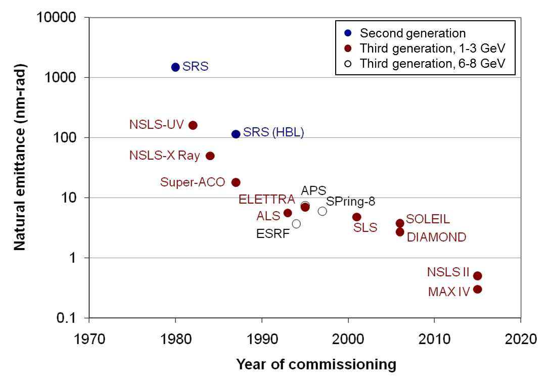
Figure 1: Natural emittance of a number of synchrotron light sources. Reductions in natural emittance have been driven by the need to produce higher radiation beam brightness for users.

There are of course ways of improving the brightness of a light source and the luminosity of a collider without reducing the emittances: in both cases, for example, the beam current could be increased. However, beam currents are generally limited by collective effects such as impedance-driven instabilities, Touschek scattering, or (for colliders) beam-beam effects. Designing and operating a storage ring for maximum performance involves a good understanding and control of effects that impact the beam emittances.

In this note, we shall consider the emittance of electron (and positron) storage rings: because of synchrotron radiation effects, lepton storage rings are able to achieve very small emittances (of order 1 nm horizontal emittance, and less than 10 pm vertical emittance). We shall begin in Section 2 by reviewing some of the key features of beam dynamics in the absence of synchrotron radiation. In particular, an important property of the dynamics in such cases is that the particle motion is symplectic: this has the consequence that the beam emittances (which characterise the phase space volume occupied by the particles in a beam) are conserved as the beam moves around the storage ring. We shall then show that, in a classical approximation, radiation effects lead to damping of the emittances. We shall derive expressions for the exponential damping times. Then, we shall discuss how quantum effects of synchrotron radiation lead to excitation of the beam emittances. As a result, the emittances of beams in electron (or positron) storage rings reach equilibrium values determined by the beam energy and lattice design.

In Section 3 we shall apply the expression for the natural emittance derived in Section 2 to particular styles of lattice design. In particular, we shall consider FODO, double bend achromat, theoretical minimum emittance, and multi-bend achromat lattices. Double bend achromats are of particular interest for light sources, because they achieve low natural emittance (leading to high brightness) while providing long, dispersion-free (or low dispersion) straight sections that are ideal locations for insertion devices such as undulators or wigglers [1]. Insertion devices are useful for providing intense beams of synchrotron radiation with specific properties.

In a planar storage ring, the vertical emittance is dominated by alignment and tuning errors, rather than by the design of the lattice. In Section 4 we shall discuss how the vertical emittance is related to a range of errors, including steering errors, tilt errors on quadrupoles and vertical alignment errors on sextupoles. Betatron coupling and vertical dispersion are important features of the dynamics in this context, and both will be discussed. Optimisation of a lattice design for a low-emittance storage ring will generally involve simulations to characterise the sensitivity of the vertical emittance to different types of machine error. For this, techniques are needed for accurate computation of the equilibrium emittances from models in which different errors can be included. We shall consider three techniques that are widely used for emittance computation, discussing the envelope method in particular in some detail. Finally, we shall mention briefly some of the issues associated with operational tuning of a storage ring for low-emittance operation.

2 Beam dynamics with synchrotron radiation

In this section, we shall review the relevant aspects of beam dynamics needed for understanding the effects of synchrotron radiation. Our focus will be on electron (or positron) synchrotron storage rings. Initially, we shall neglect radiation effects; then, we shall include the emission of synchrotron radiation as a perturbation to the motion of individual particles. This approach is valid if radiation effects are relatively weak, which means that the energy lost by a particle through radiation in one synchrotron period should be small compared to the total energy of a particle. This is almost invariably the case for practical storage rings. We shall consider only incoherent synchrotron radiation, in other words we shall assume that the motion of each particle and the radiation that it produces can be considered independently of all other particles in the beam. In some regimes (including, for example, in free electron lasers) particles generate radiation coherently, leading to a strong enhancement of the radiation produced by a beam. Generally, some special efforts are needed to achieve the generation of coherent synchrotron radiation with sufficient intensity that it has a measurable impact on the beam; we shall not discuss such situations here.

Briefly, we shall proceed as follows. The symplectic motion of particles in an accelerator (i.e. motion neglecting synchrotron radiation and collective effects) is conveniently described using action-angle variables. We shall define these variables, and use them to review the key features of particle motion in synchrotron storage rings. We shall then include the effects of synchrotron radiation, initially in a classical approximation, leading to expressions for the energy lost per turn in a storage ring, and the damping times for the horizontal, vertical and longitudinal emittances. Finally, we shall discuss the effects of quantum excitation, and derive results for the equilibrium beam emittances. These results will be used in Section 3, where we consider how the equilibrium emittances are affected by the lattice design in a storage ring.

2.1 Symplectic motion

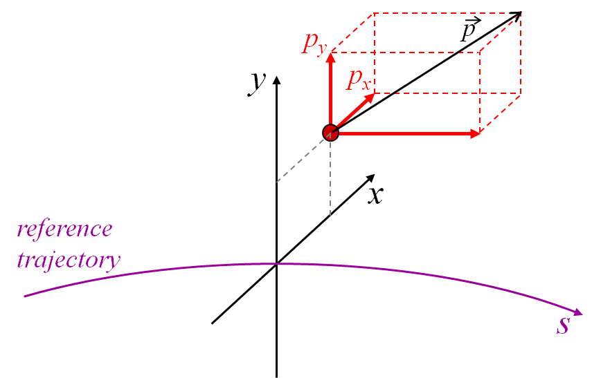
Figure 2: Co-ordinate system in an accelerator beam line. The reference trajectory can be defined arbitrarly, but is generally chosen so that it describes the trajectory of a particle with momentum equal to the reference momentum $P_{0}$. The distance along the reference trajectory is parameterised by the independent variable $s$. At any point along the reference trajectory, the transverse position of a particle is specified by Cartesian co-ordinates in a plane perpendicular to the reference trajectory.

We work in a co-ordinate system based on a reference trajectory that we define for our own convenience (see Fig. 2). The distance along the reference trajectory is specified by the independent variable $s$. For simplicity, in a planar storage ring, the reference trajectory is generally chosen to be a straight line (passing through the centres of all quadrupole and higher-order multipole magnets) everywhere except in the dipoles. In the dipoles, the reference trajectory follows the arc of a circle with radius $\rho$, such that:

$$B\rho=\frac{P_{0}}{q},$$ (1)

where $B$ is the dipole field, $P_{0}$ is the reference momentum (i.e. the momentum of particles for which the storage ring is designed) and $q$ is the particle charge. $B\rho$ is the beam rigidity.

At any point along the reference trajectory, the position of a particle is specified by the $x$ and $y$ co-ordinates in a plane perpendicular to the reference trajectory. We follow the convention in which $x$ is the horizontal (transverse) co-ordinate, and $y$ is the vertical co-ordinate.

To describe the motion of a particle, we need to give the components of the momentum of a particle, as well as its co-ordinates. In the transverse directions (i.e. in a plane perpendicular to the reference trajectory) we use the canonical momenta [2] scaled by the reference momentum $P_{0}$:

$$p_{x} = \frac{1}{P_{0}}\left(\gamma m\frac{dx}{dt}+qA_{x}\right),$$ (2)

$$p_{y} = \frac{1}{P_{0}}\left(\gamma m\frac{dy}{dt}+qA_{y}\right).$$ (3)

Here, $m$ and $q$ are the mass and charge of the particle, $\gamma$ is the relativistic factor for the particle, and $A_{x}$ and $A_{y}$ are the $x$ and $y$ components respectively of the electromagnetic vector potential. The transverse dynamics are described by giving the transverse co-ordinates and momenta as functions of $s$ (the distance along the reference trajectory).

To describe the longitudinal dynamics of a particle, we use a longitudinal co-ordinate $z$ defined by:

$$z=\beta_{0}c(t_{0}-t),$$ (4)

where $\beta_{0}$ is the normalised velocity of a particle with the reference momentum $P_{0}$, $t_{0}$ is the time at which the reference particle is at a location $s$, and $t$ is the time at which the particle of interest arrives at this location. Physically, the value of $z$ for a particle is approximately equal to the distance along the reference trajectory between the given particle and a reference particle travelling along the reference trajectory with momentum $P_{0}$ (see Fig. 3). A positive value for $z$ means that the given particle arrives at a particular location at an earlier time than the reference particle, i.e. the given particle is ahead of the reference particle.

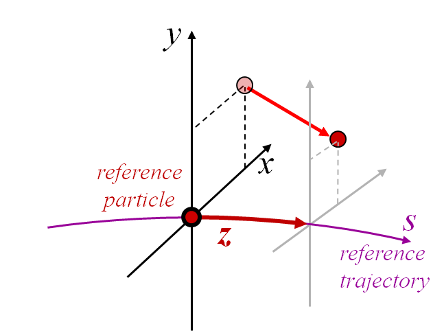
Figure 3: Longitudinal co-ordinates in an accelerator beam line. The longitudinal co-ordinate $z$ indicates the time that a particle crosses a plane perpendicular to the reference trajectory at a position $s$ along the reference trajectory.

The final dynamical variable needed to describe the motion of a particle is the energy of the particle. Rather than use the absolute energy or momentum, we use the energy deviation $\delta$, which provides a measure of the difference between the energy $E$ of a particle and the energy of a particle with the reference momentum $P_{0}$:

$$\delta=\frac{E}{P_{0}c}-\frac{1}{\beta_{0}}=\frac{1}{\beta_{0}}\left(\frac{\gamma}{\gamma_{0}}-1\right).$$ (5)

Here, $\gamma_{0}$ is the relativistic factor for a particle with momentum equal to the reference momentum. A particle with momentum equal to the reference momentum has $\delta=0$.

Using the above definitions the co-ordinates and momenta form canonical conjugate pairs:

$$(x,p_{x}),\qquad(y,p_{y}),\qquad(z,\delta).$$ (6)

This means that (continuing to neglect radiation and collective effects) the equations of motion for particles in an accelerator beam line are given by Hamilton’s equations [2], with an appropriate Hamiltonian that describes the electromagnetic fields along the beam line. In a linear approximation, the change in the values of the variables when a particle moves along a beam line can be represented by a transfer matrix, $R$:

$$\left(\begin{array}[]{c}x\\ p_{x}\\ y\\ p_{y}\\ z\\ \delta\end{array}\right)_{\!\!\!s=s_{1}}=R(s_{1};s_{0})\cdot\left(\begin{array}[]{c}x\\ p_{x}\\ y\\ p_{y}\\ z\\ \delta\end{array}\right)_{\!\!\!s=s_{0}}$$ (7)

It is a general property of Hamilton’s equations that the transfer matrix $R$ is symplectic. Mathematically, this means that $R$ satisfies the relation:

$$R^{\textrm{T}}SR=S,$$ (8)

where $S$ is the antisymmetric matrix:

$$S=\left(\begin{array}[]{cccccc}0&1&0&0&0&0\\ -1&0&0&0&0&0\\ 0&0&0&1&0&0\\ 0&0&-1&0&0&0\\ 0&0&0&0&0&1\\ 0&0&0&0&-1&0\end{array}\right).$$ (9)

The symplectic condition (8) imposes strong constraints on the dynamics. Physically, symplectic matrices preserve volumes in phase space (this result is sometimes expressed as Liouville’s theorem [2]). For example, for a linear transformation in one degree of freedom, a particular ellipse in $x$–$p_{x}$ phase space will be transformed to an ellipse with (in general) a different shape; but the area of the ellipse will remain the same. The number of invariants associated with a linear symplectic transformation is at least equal to the number of degrees of freedom in the system. Thus, for motion in three degrees of freedom, there are at least three invariants. For particles in a beam in an accelerator beam line, the invariants are associated with the emittances. If there is no coupling between the degrees of freedom (so that motion in any direction $x$, $y$ or $z$ is independent of the motion in the other two directions) then we can associate an emittance with each of the three co-ordinates, i.e. there is a horizontal emittance, a vertical emittance and a longitudinal emittance. We shall give a more formal definition of the emittances shortly.

Consider a particle moving through a periodic beam line, without coupling (i.e. a beam line with no skew quadrupoles or solenoids). After each periodic cell, we can plot the horizontal co-ordinate $x$ and momentum $p_{x}$ as a point in the horizontal phase space. After passing through many cells, observing the particle always at the corresponding locations in successive cells, and assuming that the motion of the particle is stable, we find that the points trace out an ellipse in phase space. The shape of the ellipse defines the Courant–Snyder parameters [3] in the beam line at the observation point: see Fig. 4. The area of the ellipse is a measure of the amplitude of the oscillations. We define the horizontal action $J_{x}$ of the particle such that the area of the ellipse is equal to $\pi J_{x}$.

Applying simple geometry to the phase space ellipse, we find that the action (for uncoupled motion) is related to the Cartesian variables for the particle by:

$$2J_{x}=\gamma_{x}x^{2}+2\alpha_{x}xp_{x}+\beta_{x}p_{x}^{2},$$ (10)

where the Courant–Snyder parameters satisfy the relation:

$$\beta_{x}\gamma_{x}-\alpha_{x}^{2}=1.$$ (11)

We define the horizontal angle variable $\phi_{x}$ as follows:

$$\tan\phi_{x}=-\beta_{x}\frac{p_{x}}{x}-\alpha_{x}.$$ (12)

For a particle with a particular action (i.e. on an ellipse with a given area) the angle variable specifies the position of the particle around the ellipse. The action-angle variables [2] provide an alternative to the Cartesian variables for describing the dynamics. Although we have not shown that this is the case, the action-angle variables form a canonical conjugate pair: that is, the equations of motion expressed in terms of the action-angle variables can be derived from Hamilton’s equations, using an appropriate Hamiltonian (determined as before by the electromagnetic fields along the beam line). The advantage of using action-angle variables to describe particle motion in an accelerator is that, under symplectic transport (i.e. neglecting radiation and collective effects), the action of a particle is constant. We can of course define vertical and (in a synchrotron storage ring) longitudinal action-angle variables in the same way as we defined the horizontal action-angle variables.

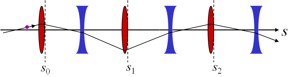
Figure 4: Ellipse in phase space defined by plotting the co-ordinate $x$ and conjugate momentum $p_{x}$ of a particle after each pass through a unit cell in a periodic beam line. The shape of the ellipse is described by the Courant–Snyder parameters $\alpha_{x}$, $\beta_{x}$ and $\gamma_{x}$; the area of the ellipse is $\pi J_{x}$, where $J_{x}$ is the action variable of the particle. The shape of the ellipse changes depending on the chosen starting position within a unit cell; the action remains the same for any given particle.

The expressions for the action (10) and the angle (12) can be inverted, to give expressions for the Cartesian co-ordinate and momentum in terms of $J_{x}$ and $\phi_{x}$:

$$x = \sqrt{2\beta_{x}J_{x}}\cos\phi_{x},$$ (13)

$$p_{x} = -\sqrt{\frac{2J_{x}}{\beta_{x}}}\left(\sin\phi_{x}+\alpha_{x}\cos\phi_{x}\right).$$ (14)

The emittance $\varepsilon_{x}$ of a bunch of particles can be defined as the average action of all particles in the bunch:

$$\varepsilon_{x}=\langle J_{x}\rangle.$$ (15)

For uncoupled motion, and assuming that the angle variables of different particles are uncorrelated, it follows from (13) and (14) that the second order moments of the particle distribution are related to the Courant–Snyder parameters and the emittance:

$$\langle x^{2}\rangle = \beta_{x}\varepsilon_{x},$$ (16)

$$\langle xp_{x}\rangle = -\alpha_{x}\varepsilon_{x},$$ (17)

$$\langle p_{x}^{2}\rangle = \gamma_{x}\varepsilon_{x}.$$ (18)

Using (11), we then find that the emittance can be expressed in terms of the second order moments as:

$$\varepsilon_{x}^{2}=\langle x^{2}\rangle\langle p_{x}^{2}\rangle-\langle xp_{x}\rangle^{2}.$$ (19)

However, we stress that this relation holds only for uncoupled motion. The expression for the emittance (15) can be generalised without too much difficulty to coupled motion (see, for example [4]), leading to normal mode emittances that are conserved under symplectic transport even where coupling is present. However, the expression for the emittance (19) is less easily generalised to include coupling, and an emittance that is defined by (19) will, in general, not be constant in a beam line where there is coupling.

2.2 Vertical damping by synchrotron radiation

So far, we have considered only symplectic transport, i.e. motion of a particle in drift spaces or in the electromagnetic fields of dipoles, quadrupoles, rf cavities etc. without any radiation. However, we know that a charged particle moving through an electromagnetic field will (in general) undergo acceleration, and a charged particle undergoing acceleration will radiate energy in the form of electromagnetic waves. We now address the question of the impact that this radiation will have on the motion of a particle in a synchrotron storage ring. We shall consider first the case of uncoupled vertical motion: for a particle in a storage ring, this turns out to be the simplest case. Since we are primarily interested in the dynamics of the particles generating the radiation, we quote a number of results regarding the properties of the radiation itself (rather than derive these results from first principles).

The first result that we quote for the properties of synchrotron radiation, is that radiation from a relativistic charged particle is emitted within a cone of opening angle of $1/\gamma$, where $\gamma$ is the relativistic factor for the particle [5]. The axis of the cone is tangent to the trajectory of the particle at the point where the radiation is emitted. For an ultra-relativistic particle, $\gamma\gg 1$, and we can assume that the radiation is emitted directly along the instantaneous direction of motion of the particle.

Consider a particle with initial momentum $P\approx P_{0}$, that emits radiation carrying momentum $dP$. The momentum of the particle after emitting radiation is:

$$P^{\prime}=P-dP\approx P\left(1-\frac{dP}{P_{0}}\right).$$ (20)

Since there is no change in direction of the particle, the vertical component of the momentum must scale in the same way as the total momentum of the particle:

$$p^{\prime}_{y}\approx p_{y}\left(1-\frac{dP}{P_{0}}\right).$$ (21)

Now we substitute this into the expression for the vertical betatron action (valid for uncoupled motion):

$$2J_{y}=\gamma_{y}y^{2}+2\alpha_{y}yp_{y}+\beta_{y}p_{y}^{2},$$ (22)

to find the change in the action resulting from the emission of radiation:

$$dJ_{y}=-\left(\alpha_{y}yp_{y}+\beta_{y}p_{y}^{2}\right)\frac{dP}{P_{0}}.$$ (23)

Note that in (23) we neglect a term that is second order in $dP/P_{0}$. This term vanishes in the classical approximation when we consider the emission of an infinitesimal amount of radiation in an infinitesimal time interval $dt$; however, we shall see later that including quantum effects, the second order term will lead to excitation of the action. Retaining for the present only the first order term in $dP/P_{0}$, averaging (23) over all particles in the beam gives:

$$\langle dJ_{y}\rangle=d\varepsilon_{y}=-\varepsilon_{y}\frac{dP}{P_{0}},$$ (24)

where we have used:

$$\langle yp_{y}\rangle = -\alpha_{y}\varepsilon_{y},$$ (25)

$$\langle p_{y}^{2}\rangle = \gamma_{y}\varepsilon_{y},$$ (26)

and:

$$\beta_{y}\gamma_{y}-\alpha_{y}^{2}=1.$$ (27)

The emittance is conserved under symplectic transport, so if the effects of radiation are ‘slow’ (i.e. the rate of change of energy from radiation is small compared to the total energy of a particle divided by the revolution period), then for a particle in a storage ring we can average the momentum loss around the ring. From (24):

$$\frac{d\varepsilon_{y}}{dt}=-\frac{\varepsilon_{y}}{T_{0}}\oint\frac{dP}{P_{0}}\approx-\frac{U_{0}}{E_{0}T_{0}}\varepsilon_{y}=-\frac{2}{\tau_{y}}\varepsilon_{y},$$ (28)

where $T_{0}$ is the revolution period, and $U_{0}$ is the energy lost through synchrotron radiation in one turn. The approximation is valid for an ultra-relativistic particle, which has $E_{0}\approx P_{0}c$. The damping time $\tau_{y}$ is defined by:

$$\tau_{y}=2\frac{E_{0}}{U_{0}}T_{0}.$$ (29)

The evolution of the emittance is given by:

$$\varepsilon_{y}(t)=\varepsilon_{y}(t=0)\exp\!\left(-2\frac{t}{\tau_{y}}\right).$$ (30)

Typically, in an electron storage ring, the damping time is of order several tens of milliseconds, while the revolution period is of the order of a microsecond. In such a case, radiation effects are indeed slow compared to the revolution frequency.

Note that we made the assumption that the momentum of the particle was close to the reference momentum, i.e. $P\approx P_{0}$. If the particle continues to radiate without any restoration of energy, we will reach a point where this assumption is no longer valid. However, electron storage rings contain rf cavities to restore the energy lost through synchrotron radiation. For a thorough analysis of synchrotron radiation effects on the vertical motion (at least, with a classical model for the radiation), we should consider the change in momentum of a particle as it moves through an rf cavity. However, in general, rf cavities are designed to provide a longitudinal electric field. This means that particles experience a change in longitudinal momentum as they pass through a cavity, without any change in transverse momentum. In other words, the vertical momentum $p_{y}$ of a particle will remain constant as the particle moves through an rf cavity, which will therefore have no effect on the emittance of the beam.

To complete our calculation of the vertical damping time, we need to find the energy lost by a particle through synchrotron radiation on each turn through the storage ring. At this point, we quote a second result from the theory of synchrotron radiation: the radiation power from a relativistic particle following a circular trajectory of radius $\rho$ is given by Liénard’s formula [5]:

$$P_{\gamma}=\frac{q^{2}c}{6\pi\epsilon_{0}}\frac{\beta^{4}\gamma^{4}}{\rho^{2}}=\frac{C_{\gamma}c}{2\pi}\frac{c^{4}P^{4}}{\rho^{2}}=\frac{C_{\gamma}}{2\pi}c^{5}q^{2}B^{2}P^{2}\approx\frac{C_{\gamma}}{2\pi}c^{3}q^{2}B^{2}E^{2},$$ (31)

where the particle has charge $q$, velocity $\beta c\approx c$, energy $E=\gamma mc^{2}$ and momentum $P=\beta\gamma mc$. The particle travels on a path with radius $\rho$ in a magnetic field of strength $B$. The approximation in the final expression of (31) is valid for ultra-relativistic particles, $\gamma\gg 1$. $\epsilon_{0}$ is the permittivity of free space, and $C_{\gamma}$ is a physical constant given by:

$$C_{\gamma}=\frac{q^{2}}{3\epsilon_{0}(mc^{2})^{4}}.$$ (32)

For electrons, $C_{\gamma}\approx 8.846\times 10^{-5}\,\textrm{m/GeV}^{3}$. Note that the radiation power has a very strong scaling with the particle mass: the larger the mass of the particle, the smaller the amount of radiation emitted. In proton storage rings, except at extremely high energy, synchrotron radiation effects are generally negligible. For a particle with the reference energy, travelling close to the speed of light along the reference trajectory, we can find the energy loss by integrating the radiation power around the ring:

$$U_{0}=\oint P_{\gamma}\,dt\approx\oint P_{\gamma}\,\frac{ds}{c}.$$ (33)

Using the expression (31) for $P_{\gamma}$, we find:

$$U_{0}\approx\frac{C_{\gamma}}{2\pi}E_{0}^{4}\oint\frac{1}{\rho^{2}}\,ds,$$ (34)

where $\rho$ is the radius of curvature of the particle trajectory, and we assume that the particle energy is equal to the reference energy $E_{0}$. For convenience, we assume that the closed orbit is the same as the reference trajectory for a particle with the reference momentum.

Following convention, we define the second synchrotron radiation integral, $I_{2}$ [6]:

$$I_{2}=\oint\frac{1}{\rho^{2}}\,ds.$$ (35)

In the ultra-relativistic limit, the energy loss per turn $U_{0}$ is written in terms of $I_{2}$ as:

$$U_{0}=\frac{C_{\gamma}}{2\pi}E_{0}^{4}I_{2}.$$ (36)

Note that $I_{2}$ is a property of the lattice (actually, a property of the reference trajectory), and does not depend on the properties of the beam. Conventionally, there are five synchrotron radiation integrals used to express the effects of synchrotron radiation on the dynamics of ultra-relativistic particles in an accelerator. The first synchrotron radiation integral is not, however, directly related to the radiation effects. It is defined as:

$$I_{1}=\oint\frac{\eta_{x}}{\rho}\,ds,$$ (37)

where $\eta_{x}$ is the horizontal dispersion. $I_{1}$ is related to the momentum compaction factor $\alpha_{p}$, which plays an important role in the longitudinal dynamics, and describes the change in the length of the closed orbit with respect to particle energy:

$$\frac{\Delta C}{C_{0}}=\alpha_{p}\delta+O(\delta^{2}).$$ (38)

The length of the closed orbit changes with energy because of dispersion in regions where the reference trajectory has some curvature (see Fig. 5):

$$dC=(\rho+x)\,d\theta=\left(1+\frac{x}{\rho}\right)\,ds.$$ (39)

If $x=\eta_{x}\delta$, then:

$$dC=\left(1+\frac{\eta_{x}\delta}{\rho}\right)\,ds.$$ (40)

The momentum compaction factor can be written:

$$\alpha_{p}=\left.\frac{1}{C_{0}}\frac{dC}{d\delta}\right|_{\delta=0}=\frac{1}{C_{0}}\oint\frac{\eta_{x}}{\rho}\,ds=\frac{I_{1}}{C_{0}}.$$ (41)

Figure 5: Change in path length of a particle following a trajectory offset from the reference trajectory. If a particle has co-ordinate $x$ and follows a path parallel to the reference trajectory, then the length of the path followed by the particle is $dC=(1+x/\rho)ds$, where $\rho$ is the radius of curvature of the reference trajectory, and $ds$ is the corresponding distance along the reference trajectory.

2.3 Horizontal damping

Analysis of the effect of synchrotron radiation on the vertical emittance was relatively straightforward. When we consider the horizontal emittance, there are three complications that we need to address. First, the horizontal motion of a particle is often strongly coupled to the longitudinal motion. We cannot treat the horizontal motion without also considering (to some extent) the longitudinal motion. Second, where the reference trajectory is curved (usually, in dipoles), the length of the path taken by a particle depends on the horizontal co-ordinate with respect to the reference trajectory. This can be a significant effect since dipoles inevitably generate dispersion (a variation of the orbit with respect to changes in particle energy), so the length of the path taken by a particle through a dipole will depend on its energy. Finally, dipole magnets are sometimes built with a gradient, in which case the vertical field seen by a particle in a dipole will depend on the horizontal co-ordinate of the particle.

Coupling between transverse and longitudinal planes in a beam line is usually represented by the dispersion, $\eta_{x}$ and $\eta_{px}$, defined by:

$$\eta_{x} = \left.\frac{dx_{\mathrm{co}}}{d\delta}\right|_{\delta=0},$$ (42)

$$\eta_{px} = \left.\frac{dp_{x,\mathrm{co}}}{d\delta}\right|_{\delta=0},$$ (43)

where $x_{\mathrm{co}}$ and $p_{x,\mathrm{co}}$ are the co-ordinate and momentum for a particle with energy deviation $\delta$ on a closed orbit. We use the horizontal action-angle variables $J_{x}$ and $\phi_{x}$ to describe the horizontal betatron oscillations of a particle with respect to the dispersive closed orbit, i.e. the closed orbit for a particle with energy deviation $\delta$. In terms of the horizontal dispersion and betatron action, the horizontal co-ordinate and momentum of a particle are given by:

$$x = \sqrt{2\beta_{x}J_{x}}\cos\phi_{x}+\eta_{x}\delta,$$ (44)

$$p_{x} = -\sqrt{\frac{2J_{x}}{\beta_{x}}}\left(\sin\phi_{x}+\alpha_{x}\cos\phi_{x}\right)+\eta_{px}\delta.$$ (45)

When a particle emits radiation, we have to take into account both the change in momentum of the particle, and the change in co-ordinate and momentum with respect to the new (dispersive) closed orbit. Note that when we analysed the vertical motion, we assumed that there was no vertical dispersion. This is the case in an ideal, planar storage ring, but as we shall discuss later, alignment errors on the magnets can lead to the generation of some vertical dispersion that depends on the errors, the effects of which cannot always be neglected.

Taking all the above effects into account for the horizontal motion, we can proceed along the same lines as for the analysis of the vertical emittance. That is, we first write down the changes in co-ordinate $x$ and momentum $p_{x}$ resulting from an emission of radiation with momentum $dP$ (taking into account the additional effects of dispersion). Then, we substitute expressions for the new co-ordinate and momentum into the expression for the horizontal betatron action, to find the change in action resulting from the radiation emission. Averaging over all particles in the beam gives the change in the emittance that results from radiation emission from each particle in the beam. Finally, we integrate around the ring (taking account of changes in path length and field strength with the horizontal position in the bends) to find the change in emittance over one turn.

Filling in the steps in this calculation, we proceed as follows. First, we note that, in the presence of dispersion, the action $J_{x}$ is written:

$$2J_{x}=\gamma_{x}\tilde{x}^{2}+2\alpha_{x}\tilde{x}\tilde{p}_{x}+\beta_{x}\tilde{p}_{x}^{2},$$ (46)

where $\tilde{x}$ and $\tilde{p}_{x}$ are the horizontal co-ordinate and momentum with respect to the dispersive closed orbit:

$$\tilde{x} = x-\eta_{x}\delta,$$ (47)

$$\tilde{p}_{x} = p_{x}-\eta_{px}\delta.$$ (48)

After emission of radiation carrying momentum $dP$, the variables change by:

$$\delta \mapsto \delta-\frac{dP}{P_{0}},$$ (49)

$$\tilde{x} \mapsto \tilde{x}+\eta_{x}\frac{dP}{P_{0}},$$ (50)

$$\tilde{p}_{x} \mapsto \tilde{p}_{x}\left(1-\frac{dP}{P_{0}}\right)+\eta_{px}\frac{dP}{P_{0}}.$$ (51)

We write the resulting change in the action as:

$$J_{x}\mapsto J_{x}+dJ_{x}.$$ (52)

The change in the horizontal action is:

$$dJ_{x}=-w_{1}\frac{dP}{P_{0}}+w_{2}\left(\frac{dP}{P_{0}}\right)^{\!2},$$ (53)

where, in the limit $\delta\to 0$:

$$w_{1}=\alpha_{x}xp_{x}+\beta_{x}p_{x}^{2}-\eta_{x}(\gamma_{x}x+\alpha_{x}p_{x})-\eta_{px}(\alpha_{x}x+\beta_{x}p_{x}),$$ (54)

and:

$$w_{2}=\frac{1}{2}\left(\gamma_{x}\eta_{x}^{2}+2\alpha_{x}\eta_{x}\eta_{px}+\beta_{x}\eta_{px}^{2}\right)-\left(\alpha_{x}\eta_{x}+\beta_{x}\eta_{px}\right)p_{x}+\frac{1}{2}\beta_{x}p_{x}^{2}.$$ (55)

Treating radiation as a classical phenomenon, we can take the limit $dP\to 0$ in the limit of small time interval, $dt\to 0$. In this approximation, the term that is second order in $dP$ vanishes, and we can write for the rate of change of the action:

$$\frac{dJ_{x}}{dt}=-w_{1}\frac{1}{P_{0}}\frac{dP}{dt}\approx-w_{1}\frac{P_{\gamma}}{P_{0}c},$$ (56)

where $P_{\gamma}$ is the rate of energy loss of the particle through synchrotron radiation (31). To find the average rate of change of horizontal action, we integrate over one revolution period:

$$\frac{dJ_{x}}{dt}=-\frac{1}{T_{0}}\oint w_{1}\frac{P_{\gamma}}{P_{0}c}\,dt.$$ (57)

It is more convenient, given a particular lattice design, to integrate over the circumference of the ring, rather than over one revolution period. However, we have to be careful changing the variable of integration (from time $t$ to distance $s$) where the reference trajectory is curved:

$$dt=\frac{dC}{c}=\left(1+\frac{x}{\rho}\right)\frac{ds}{c}.$$ (58)

So:

$$\frac{dJ_{x}}{dt}=-\frac{1}{T_{0}P_{0}c^{2}}\oint w_{1}P_{\gamma}\left(1+\frac{x}{\rho}\right)\,ds,$$ (59)

where the rate of energy loss $P_{\gamma}$ is given by (31).

We have to take into account the fact that in general, the field strength in a dipole can vary with position. To first order in $x$ we can write:

$$B=B_{0}+x\frac{\partial B}{\partial x}.$$ (60)

Substituting (60) into (31), and with the use of (54), we find (after some algebra) that, averaging over all particles in the beam:

$$\oint\left\langle w_{1}P_{\gamma}\left(1+\frac{x}{\rho}\right)\right\rangle\,ds=cU_{0}\left(1-\frac{I_{4}}{I_{2}}\right)\varepsilon_{x},$$ (61)

where the energy loss per turn $U_{0}$ is given by (36), the second synchrotron radiation integral $I_{2}$ is given by (35), and the fourth synchrotron radiation integral is $I_{4}$:

$$I_{4}=\oint\frac{\eta_{x}}{\rho}\left(\frac{1}{\rho^{2}}+2k_{1}\right)ds.$$ (62)

$k_{1}$ is the normalised quadrupole gradient in the dipole field:

$$k_{1}=\frac{q}{P_{0}}\frac{\partial B_{y}}{\partial x}.$$ (63)

Note that in (62), the dispersion and quadrupole gradient contribute to the integral only in the dipoles: in other parts of the ring, where the beam follows a straight path, the curvature $1/\rho$ is zero.

Averaging (59) over all particles in the beam and combining with (61) we have:

$$\frac{d\varepsilon_{x}}{dt}=-\frac{1}{T_{0}}\frac{U_{0}}{E_{0}}\left(1-\frac{I_{4}}{I_{2}}\right)\varepsilon_{x}.$$ (64)

Defining the horizontal damping time $\tau_{x}$:

$$\tau_{x}=\frac{2}{j_{x}}\frac{E_{0}}{U_{0}}T_{0},$$ (65)

where:

$$j_{x}=1-\frac{I_{4}}{I_{2}},$$ (66)

the evolution of the horizontal emittance can be written:

$$\frac{d\varepsilon_{x}}{dt}=-\frac{2}{\tau_{x}}\varepsilon_{x}.$$ (67)

The quantity $j_{x}$ is called the horizontal damping partition number. For most synchrotron storage ring lattices, if there is no gradient in the dipoles then $j_{x}$ is very close to 1. From (67) the horizontal emittance decays exponentially:

$$\varepsilon_{x}(t)=\varepsilon_{x}(t=0)\exp\!\left(-2\frac{t}{\tau_{x}}\right).$$ (68)

2.4 Longitudinal damping

So far we have considered only the effects of synchrotron radiation on the transverse motion, but there are also effects on the longitudinal motion. Generally, synchrotron oscillations are treated differently from betatron oscillations because in one revolution of a typical storage ring, particles complete many betatron oscillations but only a fraction of a synchrotron oscillation. In other words, the betatron tunes are $\nu_{\beta}\gg 1$, but the synchrotron tune is $\nu_{s}\ll 1$. To find the effects of radiation on synchrotron motion, we proceed as follows. We first write down the equations of motion (for the dynamical variables $z$ and $\delta$) for a particle performing synchrotron motion, including the radiation energy loss. Then, we express the energy loss per turn as a function of the energy deviation of the particle. This introduces a damping term into the equations of motion. Finally, solving the equations of motion gives synchrotron oscillations (as expected) with amplitude that decays exponentially.

The changes in energy deviation $\delta$ and longitudinal co-ordinate $z$ for a particle in one turn around a storage ring are given by:

$$\Delta\delta = \frac{qV_{\textrm{rf}}}{E_{0}}\sin\!\left(\phi_{s}-\frac{\omega_{\textrm{rf}}z}{c}\right)-\frac{U}{E_{0}},$$ (69)

$$\Delta z = -\alpha_{p}C_{0}\delta,$$ (70)

where $V_{\textrm{rf}}$ is the rf voltage, $\omega_{\textrm{rf}}$ the rf frequency, $E_{0}$ is the reference energy of the beam, $\phi_{s}$ is the nominal rf phase, and $U$ (which may be different from $U_{0}$) is the energy lost by the particle through synchrotron radiation. Strictly speaking, since the longitudinal co-ordinate $z$ is a measure of the time at which a particle arrives at a particular location in the ring, changes in $z$ with respect to energy should be written in terms of the phase slip factor $\eta_{p}$, which describes the change in revolution period with respect to changes in energy, rather than in terms of the momentum compaction factor $\alpha_{p}$. The phase slip factor and the momentum compaction factor are related by (see, for example [7]):

$$\eta_{p}=\alpha_{p}-\frac{1}{\gamma_{0}^{2}},$$ (71)

where $\gamma_{0}$ is the relativistic factor for a particle with the reference momentum. But for a storage ring operating a long way above transition (which is the situation we shall assume here) $\alpha_{p}\gg 1/\gamma_{0}^{2}$, so $\eta_{p}\approx\alpha_{p}$. It is slightly more convenient to work with the momentum compaction factor, since this depends (essentially) on just the geometry of the lattice and the optical functions (in particular, the dispersion); whereas the phase slip factor depends also on the beam energy.

If the revolution period in the storage ring is $T_{0}$, then we can write the longitudinal equations of motion for the particle:

$$\frac{d\delta}{dt} = \frac{qV_{\textrm{rf}}}{E_{0}T_{0}}\sin\!\left(\phi_{s}-\frac{\omega_{\textrm{rf}}z}{c}\right)-\frac{U}{E_{0}T_{0}},$$ (72)

$$\frac{dz}{dt} = -\alpha_{p}c\delta.$$ (73)

To solve these equations, we have to make some assumptions. First, we assume that $z$ is small compared to the rf wavelength:

$$\frac{\omega_{\textrm{rf}}|z|}{c}\ll 1.$$ (74)

The synchrotron radiation power produced by a particle depends on the energy of the particle. We assume that the energy deviation is small, $|\delta|\ll 1$, so we can work to first order in $\delta$:

$$U=U_{0}+\Delta E\left.\frac{dU}{dE}\right|_{E=E_{0}}=U_{0}+E_{0}\delta\left.\frac{dU}{dE}\right|_{E=E_{0}}.$$ (75)

Finally, we assume that the rf phase $\phi_{s}$ is set so that for $z=\delta=0$, the rf cavity restores exactly the amount of energy lost by synchrotron radiation. With these assumptions, the equations of motion become:

$$\frac{d\delta}{dt} = -\frac{qV_{\textrm{rf}}}{E_{0}T_{0}}\cos(\phi_{s})\frac{\omega_{\textrm{rf}}}{c}z-\frac{1}{T_{0}}\delta\left.\frac{dU}{dE}\right|_{E=E_{0}},$$ (76)

$$\frac{dz}{dt} = -\alpha_{p}c\delta.$$ (77)

Taking the derivative of (76) with respect to $t$, and substituting for $dz/dt$ from (77) gives:

$$\frac{d^{2}\delta}{dt^{2}}+2\alpha_{E}\frac{d\delta}{dt}+\omega^{2}_{s}\delta=0.$$ (78)

This is the equation for a damped harmonic oscillator, with frequency $\omega_{s}$ and damping constant $\alpha_{E}$ given by:

$$\omega_{s}^{2} = -\frac{qV_{\textrm{rf}}}{E_{0}}\cos(\phi_{s})\frac{\omega_{\textrm{rf}}}{T_{0}}\alpha_{p},$$ (79)

$$\alpha_{E} = \frac{1}{2T_{0}}\left.\frac{dU}{dE}\right|_{E=E_{0}}.$$ (80)

If $\alpha_{E}\ll\omega_{s}$, the energy deviation and longitudinal co-ordinate damp as:

$$\delta(t) = \delta_{0}\exp(-\alpha_{E}t)\sin(\omega_{s}t-\theta_{0}),$$ (81)

$$z(t) = \frac{\alpha_{p}c}{\omega_{s}}\delta_{0}\exp(-\alpha_{E}t)\cos(\omega_{s}t-\theta_{0}).$$ (82)

where $\delta_{0}$ is a constant (the amplitude of the oscillation in $\delta$ at $t=0$), and $\theta_{0}$ is a fixed phase (the phase of the oscillation at $t=0$).

To find an explicit expression for the damping constant $\alpha_{E}$, we need to know how the energy loss per turn $U$ depends on the energy deviation $\delta$. The total energy lost per turn by a particle is found by integrating the synchrotron radiation power over one revolution period:

$$U=\oint P_{\gamma}\,dt.$$ (83)

To convert this to an integral over the circumference, we should recall that the path length depends on the energy deviation; so a particle with a higher energy takes longer to travel around the lattice:

$$dt=\frac{dC}{c}=\frac{1}{c}\left(1+\frac{x}{\rho}\right)ds=\frac{1}{c}\left(1+\frac{\eta_{x}\delta}{\rho}\right)\,ds.$$ (84)

Therefore, the radiation energy loss per turn is:

$$U=\frac{1}{c}\oint P_{\gamma}\left(1+\frac{\eta_{x}\delta}{\rho}\right)\,ds.$$ (85)

Using (31), we find after some algebra:

$$\left.\frac{dU}{dE}\right|_{E=E_{0}}=j_{z}\frac{U_{0}}{E_{0}},$$ (86)

where $U_{0}$ is given by (36), and the longitudinal damping partition number $j_{z}$ is:

$$j_{z}=2+\frac{I_{4}}{I_{2}}.$$ (87)

$I_{2}$ and $I_{4}$ are the same synchrotron radiation integrals that we saw before, in (35) and (62). Finally, we can write the longitudinal damping time:

$$\tau_{z}=\frac{1}{\alpha_{E}}=\frac{2}{j_{z}}\frac{E_{0}}{U_{0}}T_{0}.$$ (88)

Neglecting coupling, the longitudinal emittance can be given by a similar expression to the horizontal and vertical emittance:

$$\varepsilon_{z}=\sqrt{\langle z^{2}\rangle\langle\delta^{2}\rangle-\langle z\delta\rangle^{2}}.$$ (89)

Even where dispersion is present, so that the horizontal and longitudinal motion are coupled, the expression (89) can provide a useful definition of the longitudinal emittance, since the longitudinal variables usually have a much weaker dependence on the transverse variables, than the transverse variables have on the longitudinal. Since the amplitudes of the synchrotron oscillations decay with time constant $\tau_{z}$, the damping of the longitudinal emittance can be written:

$$\varepsilon_{z}(t)=\varepsilon_{z}(t=0)\exp\!\left(-2\frac{t}{\tau_{z}}\right).$$ (90)

It is worth commenting on the fact that the horizontal, vertical and longitudinal emittances are all damped by synchrotron radiation with exponential damping times that depend on the beam energy and the rate at which particles lose energy through synchrotron radiation. In the case of the horizontal and longitudinal emittances, there is an additional factor in the expressions for the damping times that depends on details of the lattice, or, more precisely, on the properties of the dipoles. The additional factors are given by the damping partition numbers $j_{x}$ and $j_{z}$. From (66) and (87), we see that:

$$j_{x}+j_{z}=3.$$ (91)

In general, there can also be a vertical damping partition number $j_{y}$, although in the simple case we have considered here (of a perfectly planar storage ring) $j_{y}=1$. A more general analysis would lead to the result:

$$j_{x}+j_{y}+j_{z}=4,$$ (92)

which is known as the Robinson damping theorem [8]. The significance of this result is that while it is possible (for example, by changing the field gradient in the dipoles) to ‘shift’ the radiation damping between the different degrees of freedom, the overall amount of damping is fixed. In a planar storage ring, for example, one can reduce the horizontal damping time, but only at the expense of increasing the longitudinal damping time.

In a typical storage ring, the dispersion in the dipoles is small compared to the bending radius of the dipoles, that is:

$$\frac{\eta_{x}}{\rho}\ll 1.$$ (93)

Then, if there is no quadrupole component in the dipoles (so that $k_{1}=0$ in the dipoles), comparing (35) and (62) leads to:

$$\frac{I_{4}}{I_{2}}\ll 1,$$ (94)

in which case:

$$j_{x} \approx 1,$$ (95)

$$j_{z} \approx 2.$$ (96)

The horizontal damping time is approximately equal to the vertical damping time; the longitudinal damping time is about half the vertical damping time. Typical values for the damping times in medium energy synchrotron light sources are some tens of milliseconds, or a few thousand turns.

2.5 Quantum excitation

So far, we have assumed a purely classical model for the radiation, in which energy can be radiated in arbitrarily small amounts. From the expressions for the evolutions of the emittances (30), (68) and (90), we see that if radiation was a purely classical process, the emittances would damp towards zero. However, quantum effects mean that radiation is emitted in discrete units (photons). As we shall see, this induces some ‘noise’ on the beam, known as quantum excitation, the effect of which is to increase the emittance. The beam in an electron (or positron) storage ring will eventually reach an equilibrium distribution determined by a balance between the radiation damping and the quantum excitation. In the remainder of this section, we shall derive expressions for the rate of quantum excitation and for the equilibrium emittances in an electron storage ring.

In deriving the equation of motion (59) for the action of a particle emitting synchrotron radiation, we made the (classical) approximation that in a time interval $dt$, the momentum $dP$ of the radiation emitted goes to zero as $dt$ goes to zero. In reality, emission of radiation is quantized, so we are prevented from taking the limit $dP\to 0$. The equation of motion for the action (56) should then be written:

$$\frac{dJ_{x}}{dt}=-\frac{w_{1}}{P_{0}c}\int_{0}^{\infty}\dot{N}(u)\,u\,du+\frac{w_{2}}{P_{0}^{2}c^{2}}\int_{0}^{\infty}\dot{N}(u)\,u^{2}\,du,$$ (97)

where $\dot{N}(u)$ is the number of photons emitted per unit time in the energy range from $u$ to $u+du$. The first term on the right hand side of (97) just gives the same radiation damping as in the classical approximation; the second term is an excitation term that we previously neglected.

To find an explicit expression for the rate of change of the action in terms of the beam and lattice parameters, we need to find expressions for the integrals $\int\dot{N}(u)\,u\,du$ and $\int\dot{N}(u)\,u^{2}\,du$. The required expressions can be found from the spectral distribution of synchrotron radiation from a dipole magnet, which is another result that we quote from synchrotron radiation theory. The spectral distribution of radiation from a dipole magnet is given by [5]:

$$\frac{d\mathcal{P}}{d\vartheta}=\frac{9\sqrt{3}}{8\pi}P_{\gamma}\vartheta\int_{\vartheta}^{\infty}K_{5/3}(x)\,dx,$$ (98)

where $d\mathcal{P}/d\vartheta$ is the energy radiated per unit time per unit frequency range, and $\vartheta=\omega/\omega_{c}$ is the radiation frequency $\omega$ divided by the critical frequency $\omega_{c}$:

$$\omega_{c}=\frac{3}{2}\frac{\gamma^{3}c}{\rho}.$$ (99)

$P_{\gamma}$ is the total energy radiated per unit time (31), and $K_{5/3}(x)$ is a modified Bessel function. Since the energy of a photon of frequency $\omega$ is $u=\hbar\omega$, it follows that:

$$\dot{N}(u)\,du=\frac{1}{\hbar\omega}\frac{d\mathcal{P}}{d\vartheta}\,d\vartheta.$$ (100)

Using (98) and (100), we find:

$$\int_{0}^{\infty}\dot{N}(u)\,u\,du=P_{\gamma},$$ (101)

and:

$$\int_{0}^{\infty}\dot{N}(u)\,u^{2}\,du=2C_{q}\gamma^{2}\frac{E_{0}}{\rho}P_{\gamma}.$$ (102)

$C_{q}$ is a constant given by:

$$C_{q}=\frac{55}{32\sqrt{3}}\frac{\hbar}{mc}.$$ (103)

For electrons (or positrons) $C_{q}\approx 3.832\times 10^{-13}\,\mathrm{m}$.

The next step is to substitute for the integrals in (97) from (101) and (102), substitute for $w_{1}$ and $w_{2}$ from (54) and (55), and average over the circumference of the ring. This gives an expression for the evolution of the horizontal action (for $x\ll\eta_{x}$ and $p_{x}\ll\eta_{px}$):

$$\frac{d\varepsilon_{x}}{dt}=-\frac{2}{\tau_{x}}\varepsilon_{x}+\frac{2}{j_{x}\tau_{x}}C_{q}\gamma^{2}\frac{I_{5}}{I_{2}},$$ (104)

where the fifth synchrotron radiation integral $I_{5}$ is given by:

$$I_{5}=\oint\frac{\mathcal{H}_{x}}{|\rho^{3}|}\,ds.$$ (105)

The $\mathcal{H}$ function ($\mathcal{H}_{x}$) is given by:

$$\mathcal{H}_{x}=\gamma_{x}\eta_{x}^{2}+2\alpha_{x}\eta_{x}\eta_{px}+\beta_{x}\eta_{px}^{2}.$$ (106)

The damping time and horizontal damping partition number are given, as before, by (65) and (66). Note that the excitation term is independent of the emittance: the quantum excitation does not simply modify the damping time, but leads to a non-zero equilibrium emittance. The equilibrium emittance $\varepsilon_{0}$ is determined by the condition:

$$\left.\frac{d\varepsilon_{x}}{dt}\right|_{\varepsilon_{x}=\varepsilon_{0}}=0,$$ (107)

and is given by:

$$\varepsilon_{0}=C_{q}\gamma^{2}\frac{I_{5}}{j_{x}I_{2}}.$$ (108)

Note that $\varepsilon_{0}$ is determined by the beam energy, the lattice functions (Courant–Snyder parameters and dispersion) in the dipoles, and the bending radius in the dipoles. We shall discuss how the design of the lattice affects the value of $I_{5}$ (and hence, the equilibrium horizontal emittance) in Section 3. The equilibrium horizontal emittance (108) determined by radiation is sometimes called the natural emittance of the lattice, since it includes only the most fundamental effects that contribute to the emittance: radiation damping and quantum excitation. Other phenomena (such as impedance or scattering effects) can lead to some increase in the equilibrium emittance actually achieved in a storage ring, compared to the natural emittance. Typically, third generation synchrotron light sources have natural emittances of order of a few nanometres. With beta functions of a few metres, this implies horizontal beam sizes of tens of microns (in the absence of dispersion).

In many storage rings, the vertical dispersion in the absence of alignment, steering and coupling errors is zero, so that $\mathcal{H}_{y}=0$. However, the equilibrium vertical emittance is larger than zero, because the vertical opening angle of the radiation excites some vertical betatron oscillations. The fundamental lower limit on the vertical emittance, from the opening angle of the synchrotron radiation, is given by [9]:

$$\varepsilon_{y}=\frac{13}{55}\frac{C_{q}}{j_{y}I_{2}}\oint\frac{\beta_{y}}{|\rho^{3}|}\,ds.$$ (109)

In most storage rings, this is an extremely small value, typically four orders of magnitude smaller than the natural (horizontal) emittance. In practice, the vertical emittance is dominated by magnet alignment errors. Storage rings typically operate with a vertical emittance that is of order 1% of the horizontal emittance, but many can achieve emittance ratios somewhat smaller than this. We shall discuss the vertical emittance in more detail in Section 4.

Figure 6: Change in longitudinal phase space variables for a particle emitting a photon carrying energy $u$. As a result of the photon emission, there is a change in amplitude of the synchrotron oscillations (represented by the ellipses) performed by the particle as it moves around the storage ring.

Quantum effects excite longitudinal emittance as well as transverse emittance. Consider a particle with longitudinal co-ordinate $z$ and energy deviation $\delta$, which emits a photon of energy $u$ (see Fig. 6). The co-ordinate and energy deviation after emission of the photon are given by:

$$\delta^{\prime} = \delta_{0}^{\prime}\sin\theta^{\prime}=\delta_{0}\sin\theta-\frac{u}{E_{0}},$$ (110)

$$z^{\prime} = \frac{\alpha_{p}c}{\omega_{s}}\delta_{0}^{\prime}\cos\theta^{\prime}=\frac{\alpha_{p}c}{\omega_{s}}\delta_{0}\cos\theta.$$ (111)

Therefore:

$$\delta_{0}^{\prime 2}=\delta_{0}^{2}-2\delta_{0}\frac{u}{E_{0}}\sin\theta+\frac{u^{2}}{E_{0}^{2}}.$$ (112)

Averaging over the bunch gives:

$$\Delta\sigma_{\delta}^{2}=\frac{\langle u^{2}\rangle}{2E_{0}^{2}},$$ (113)

where:

$$\sigma_{\delta}^{2}=\langle\delta^{2}\rangle=\frac{1}{2}\langle\delta_{0}^{2}\rangle.$$ (114)

Including radiation damping, the energy spread evolves as:

$$\frac{d\sigma_{\delta}^{2}}{dt}=\frac{1}{2E_{0}^{2}}\frac{1}{C_{0}}\oint dC\,\int_{0}^{\infty}du\,\dot{N}(u)u^{2}-\frac{2}{\tau_{z}}\sigma_{\delta}^{2},$$ (115)

where we have averaged the radiation effects around the ring by integrating over the circumference. Using (102) for $\int\dot{N}(u)u^{2}\,du$, we find:

$$\frac{d\sigma_{\delta}^{2}}{dt}=C_{q}\gamma^{2}\frac{2}{j_{z}\tau_{z}}\frac{I_{3}}{I_{2}}-\frac{2}{\tau_{z}}\sigma_{\delta}^{2}.$$ (116)

The equilibrium energy spread is given by $d\sigma_{\delta}^{2}/dt=0$:

$$\sigma_{\delta 0}^{2}=C_{q}\gamma^{2}\frac{I_{3}}{j_{z}I_{2}},$$ (117)

where the third synchrotron radiation integral $I_{3}$ is defined:

$$I_{3}=\oint\frac{1}{|\rho^{3}|}\,ds.$$ (118)

The equilibrium energy spread $\sigma_{\delta 0}$ determined by radiation effects is often referred to as the natural energy spread, since collective effects can often lead to an increase in the energy spread with increasing bunch charge. Note that the natural energy spread is determined essentially by the beam energy and by the bending radii of the dipoles; rather counterintuitively, it does not depend on the rf parameters (either the voltage or the frequency). On the other hand, the bunch length does have a dependence on the rf. The ratio of the bunch length $\sigma_{z}$ to the energy spread $\sigma_{\delta}$ in a matched distribution (i.e. a distribution that is unchanged after one complete revolution around the ring) can be determined from the shape of the ellipse in longitudinal phase space followed by a particle obeying the longitudinal equations of motion (72) and (73). Neglecting radiation effects (which can be assumed to be small) the result is:

$$\sigma_{z}=\frac{\alpha_{p}c}{\omega_{s}}\sigma_{\delta}.$$ (119)

We can increase the synchrotron frequency $\omega_{s}$, and hence reduce the bunch length, by increasing the rf voltage, or by increasing the rf frequency.

2.6 Summary of radiation damping and quantum excitation

To summarise, including the effects of radiation damping and quantum excitation, the emittances (in each of the three degrees of freedom) evolve with time as:

$$\varepsilon(t)=\varepsilon(t=0)\exp\left(-2\frac{t}{\tau}\right)+\varepsilon(t=\infty)\left[1-\exp\left(-2\frac{t}{\tau}\right)\right],$$ (120)

where $\varepsilon(t=0)$ is the initial emittance (for example, of a beam as it is injected into the storage ring), and $\varepsilon(t=\infty)$ is the equilibrium emittance determined by the balance between radiation damping and quantum excitation. The damping times are given by:

$$j_{x}\tau_{x}=j_{y}\tau_{y}=j_{z}\tau_{z}=2\frac{E_{0}}{U_{0}}T_{0},$$ (121)

where the damping partition numbers are given by:

$$j_{x}=1-\frac{I_{4}}{I_{2}},\qquad j_{y}=1,\qquad j_{z}=2+\frac{I_{4}}{I_{2}}.$$ (122)

The energy loss per turn is given by:

$$U_{0}=\frac{C_{\gamma}}{2\pi}E_{0}^{4}I_{2},$$ (123)

where for electrons (or positrons) $C_{\gamma}\approx 8.846\times 10^{-5}\textrm{ m/GeV}^{3}.$ The natural emittance is:

$$\varepsilon_{0}=C_{q}\gamma^{2}\frac{I_{5}}{j_{x}I_{2}},$$ (124)

where for electrons (or positrons) $C_{q}\approx 3.832\times 10^{-13}\textrm{ m}.$ The natural rms energy spread and bunch length are given by:

$$\sigma_{\delta}^{2} = C_{q}\gamma^{2}\frac{I_{3}}{j_{z}I_{2}},$$ (125)

$$\sigma_{z} = \frac{\alpha_{p}c}{\omega_{s}}\sigma_{\delta}.$$ (126)

The momentum compaction factor is:

$$\alpha_{p}=\frac{I_{1}}{C_{0}}.$$ (127)

The synchrotron frequency and synchronous phase are given by:

$$\omega_{s}^{2} = -\frac{qV_{\textrm{rf}}}{E_{0}}\frac{\omega_{\textrm{rf}}}{T_{0}}\alpha_{p}\cos\phi_{s},$$ (128)

$$\sin\phi_{s} = \frac{U_{0}}{qV_{\textrm{rf}}}.$$ (129)

Finally, the synchrotron radiation integrals are:

$$I_{1} = \oint\frac{\eta_{x}}{\rho}\,ds,$$ (130)

$$I_{2} = \oint\frac{1}{\rho^{2}}\,ds,$$ (131)

$$I_{3} = \oint\frac{1}{|\rho|^{3}}\,ds,$$ (132)

$$I_{4} = \oint\frac{\eta_{x}}{\rho}\left(\frac{1}{\rho^{2}}+2k_{1}\right)\,ds,\qquad k_{1}=\frac{e}{P_{0}}\frac{\partial B_{y}}{\partial x},$$ (133)

$$I_{5} = \oint\frac{\mathcal{H}_{x}}{|\rho|^{3}}\,ds,\qquad\mathcal{H}_{x}=\gamma_{x}\eta_{x}^{2}+2\alpha_{x}\eta_{x}\eta_{px}+\beta_{x}\eta_{px}^{2}.$$ (134)

3 Equilibrium emittance and storage ring lattice design

In this section, we shall derive expressions for the natural emittance in four types of lattices: FODO, double bend achromat (DBA), multi-bend achromat (including the triple bend achromat) and theoretical minimum emittance (TME) lattices. We shall also consider how the emittance of an achromat may be reduced by ‘detuning’ the lattice from the strict achromat conditions.

Recall that the natural emittance in a storage ring is given by (108):

$$\varepsilon_{0}=C_{q}\gamma^{2}\frac{I_{5}}{j_{x}I_{2}},$$ (135)

where $C_{q}$ is a physical constant, $\gamma$ is the relativistic factor, $j_{x}$ is the horizontal damping partition number, and $I_{5}$ and $I_{2}$ are synchrotron radiation integrals. Note that $j_{x}$, $I_{5}$ and $I_{2}$ are all fixed by the layout of the lattice and the optics, and are independent of the beam energy. In most storage rings, if the bends have no quadrupole component, the damping partition number $j_{x}\approx 1$. In that case, to find the natural emittance we just need to evaluate the two synchrotron radiation integrals $I_{2}$ and $I_{5}$. If we know the strength and length of all the dipoles in the lattice, it is straightforward to calculate $I_{2}$. For example, if all the bends are identical, then in a complete ring (total bending angle = 2$\pi$):

$$I_{2}=\oint\frac{1}{\rho^{2}}ds=\oint\frac{B}{(B\rho)}\frac{ds}{\rho}=\frac{2\pi B}{(B\rho)}\approx 2\pi\frac{cB}{E/q},$$ (136)

where $E$ is the beam energy, and $q$ is the particle charge. Evaluating $I_{5}$ is more complicated: it depends on the lattice functions.

3.1 FODO lattice

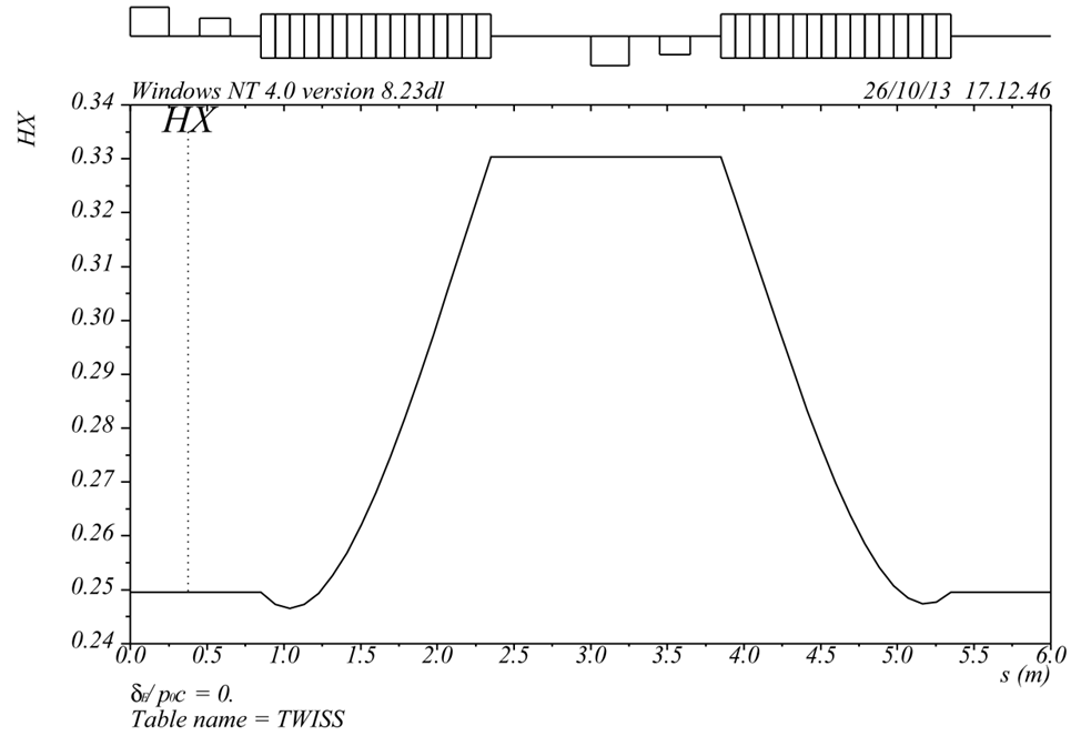
Figure 7: Lattice functions in a FODO cell. Top: Courant–Snyder parameters and dispersion. Bottom: $\mathcal{H}$ function. In this case, the phase advance is 90^∘, the dipoles are 1.5 m long and have bending angle 2$\pi$/32. Notice that the value of the $\mathcal{H}$ function is constant except in the dipoles: this is a general property of this function.

Let us consider the case of a FODO lattice. The lattice functions in a typical FODO cell are shown in Fig. 7. To simplify the system, we use the following approximations. First, we assume that the quadrupoles can be represented by thin lenses. Second, we assume that the space between the quadrupoles is completely filled by the dipoles. This is clearly not a realistic assumption, but it does allow us to derive some useful (and reasonably accurate) formulae. With these approximations, the lattice functions (Courant–Snyder parameters and dispersion) are completely determined by the focal length $f$ of the quadrupoles and the bending radius $\rho$ and length $L$ of the dipoles, and can be calculated using standard techniques.

Suppose that $R_{\textrm{cell}}$ is the transfer matrix for the horizontal motion in one complete periodic cell of a lattice. $R_{\textrm{cell}}$ may be constructed by multiplying the transfer matrices $R$ for individual components in the beam line. For example, for a thin quadrupole of focal length $f$:

$$R_{\textrm{quad}}=\left(\begin{array}[]{cc}1&0\\ -1/f&1\end{array}\right).$$ (137)

For a dipole of bending radius $\rho$ and length $L$, the transfer matrix is:

$$R_{\textrm{dip}}=\left(\begin{array}[]{cc}\cos\frac{L}{\rho}&\rho\sin\frac{L}{\rho}\\ -\frac{1}{\rho}\sin\frac{L}{\rho}&\cos\frac{L}{\rho}\end{array}\right).$$ (138)

The Courant–Snyder parameters at any point in the beam line can be found first by multiplying the transfer matrices $R$ for the individual components to give the transfer matrix $R_{\textrm{cell}}$ for the periodic cell starting from the chosen point, and then writing the complete transfer matrix in the form:

$$R_{\textrm{cell}}=\left(\begin{array}[]{cc}\cos\mu_{x}+\alpha_{x}\sin\mu_{x}&\beta_{x}\sin\mu_{x}\\ -\gamma_{x}\sin\mu_{x}&\cos\mu_{x}-\alpha_{x}\sin\mu_{x}\end{array}\right),$$ (139)

where $\mu_{x}$ is the phase advance. The dispersion describes the periodic trajectory of an (off-energy) particle through a periodic cell, and can be found at any point by solving the condition:

$$\left(\begin{array}[]{c}\eta_{x}\\ \eta_{px}\end{array}\right)=R_{\textrm{cell}}^{\eta}\left(\begin{array}[]{c}\eta_{x}\\ \eta_{px}\end{array}\right)+d_{\textrm{cell}}^{\eta},$$ (140)

where $R_{\textrm{cell}}^{\eta}$ is a matrix representing the first order terms in the map (for a complete cell) for the dispersion, and $d_{\textrm{cell}}^{\eta}$ is a vector representing the zeroth order terms. The map for a complete cell is found, as usual, by composing the maps for individual elements. For a quadrupole, the map for the dispersion is the same as the map for the dynamical variables; for a dipole, there are additional zeroth order terms:

$$\left(\begin{array}[]{c}\eta_{x}\\ \eta_{px}\end{array}\right)_{\!\!s_{0}+L}=R_{\textrm{dip}}\left(\begin{array}[]{c}\eta_{x}\\ \eta_{px}\end{array}\right)_{\!\!s_{0}}+\left(\begin{array}[]{c}\rho(1-\cos\frac{L}{\rho})\\ \sin\frac{L}{\rho}\end{array}\right).$$ (141)

Using the above results, we find that in terms of $f$, $\rho$ and $L$, the horizontal beta function at the horizontally focusing quadrupole in a FODO cell is given by:

$$\beta_{x}=\frac{4f\rho\sin\theta(2f\cos\theta+\rho\sin\theta)}{\sqrt{16f^{4}-[\rho^{2}-(4f^{2}+\rho^{2})\cos 2\theta]^{2}}},$$ (142)

where $\theta=L/\rho$ is the bending angle of a single dipole. The dispersion at a horizontally focusing quadrupole is given by:

$$\eta_{x}=\frac{2f\rho(2f+\rho\tan\frac{\theta}{2})}{4f^{2}+\rho^{2}}.$$ (143)

By symmetry, at the centre of a quadrupole, $\alpha_{x}=\eta_{px}=0$. Given the lattice functions at any point in the lattice, we can evolve the functions through the lattice, using the transfer matrices $R$. For the Courant–Snyder parameters:

$$A(s_{1})=RA(s_{0})R^{\textrm{T}},$$ (144)

where $R=R(s_{1};s_{0})$ is the transfer matrix from $s_{0}$ to $s_{1}$, $R^{\textrm{T}}$ is the transpose of $R$, and:

$$A=\left(\begin{array}[]{cc}\beta_{x}&-\alpha_{x}\\ -\alpha_{x}&\gamma_{x}\end{array}\right).$$ (145)

The dispersion can be evolved (over a distance $L$, with constant bending radius $\rho$) using (141).

We now have all the information we need to find an expression for $I_{5}$ in the FODO cell. However, the algebra is rather formidable. The result is most easily expressed as a power series in the dipole bending angle, $\theta$:

$$\frac{I_{5}}{I_{2}}=\left(4+\frac{\rho^{2}}{f^{2}}\right)^{\!\!-\frac{3}{2}}\left(8-\frac{\rho^{2}}{2f^{2}}\theta^{2}+O(\theta^{4})\right).$$ (146)

For small $\theta$, the expression for $I_{5}/I_{2}$ can be written:

$$\frac{I_{5}}{I_{2}}\approx\left(1-\frac{\rho^{2}}{16f^{2}}\theta^{2}\right)\left(1+\frac{\rho^{2}}{4f^{2}}\right)^{\!\!-\frac{3}{2}}=\left(1-\frac{L^{2}}{16f^{2}}\right)\left(1+\frac{\rho^{2}}{4f^{2}}\right)^{\!\!-\frac{3}{2}}.$$ (147)

This can be further simplified if $\rho\gg 2f$ (which is often the case):

$$\frac{I_{5}}{I_{2}}\approx\left(1-\frac{L^{2}}{16f^{2}}\right)\frac{8f^{3}}{\rho^{3}},$$ (148)

and still further simplified if $4f\gg L$ (which is less often the case):

$$\frac{I_{5}}{I_{2}}\approx\frac{8f^{3}}{\rho^{3}}.$$ (149)

The ratio $I_{5}/I_{2}$ is plotted for a FODO cell as a function of the phase advance in Fig. 8. Making the approximation $j_{x}\approx 1$ (since we assume that there is no quadrupole component in the dipole), and writing $\rho=L/\theta$, we have:

$$\varepsilon_{0}\approx C_{q}\gamma^{2}\left(\frac{2f}{L}\right)^{\!\!3}\theta^{3}.$$ (150)

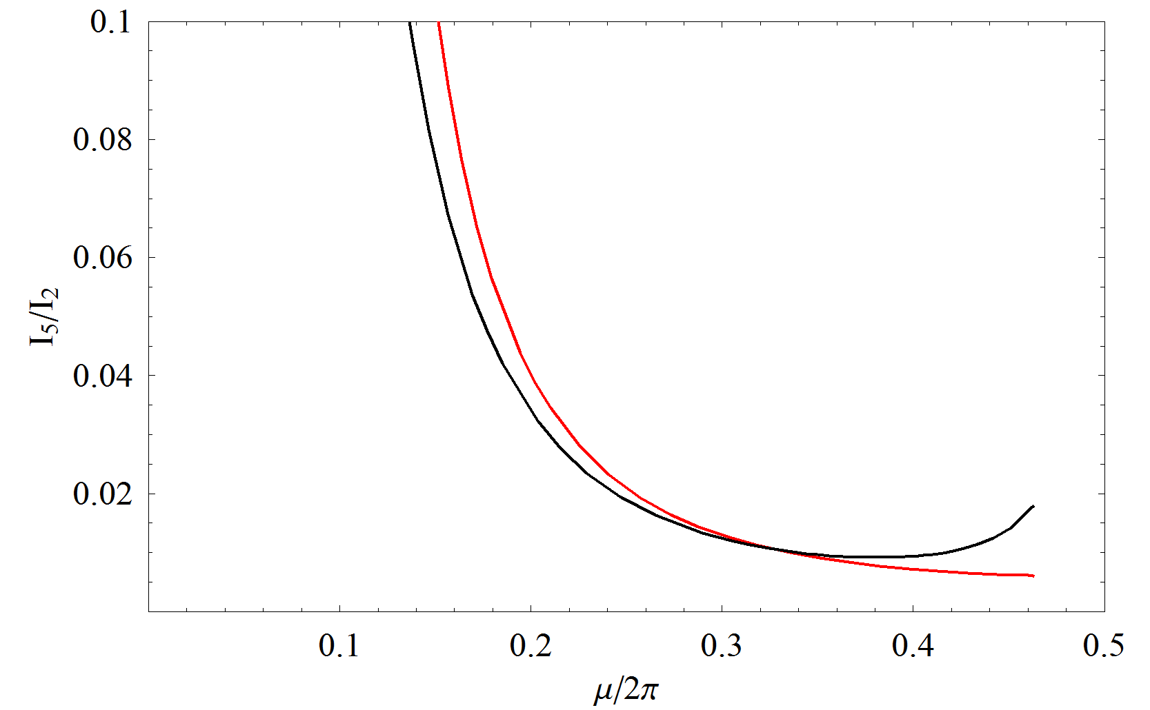
Figure 8: Ratio of synchrotron radiation integrals $I_{5}/I_{2}$ in a FODO cell, as a function of the phase advance. The black line shows the exact value, while the red line shows the value calculated using the approximation (148).

Notice how the emittance scales with the beam and lattice parameters. The emittance is proportional to the square of the energy and to the cube of the bending angle. Increasing the number of cells in a complete circular lattice reduces the bending angle of each dipole, and reduces the emittance. The emittance is proportional to the cube of the quadrupole focal length: stronger focusing results in lower emittance. Finally, the emittance is inversely proportional to the cube of the cell length.

The phase advance in a FODO cell is given by:

$$\cos\mu_{x}=1-\frac{L^{2}}{2f^{2}}.$$ (151)

This means that a stable lattice must have:

$$\frac{f}{L}\geq\frac{1}{2}.$$ (152)

In the limiting case, $\mu_{x}=180^{\circ}$, and $f$ has the minimum value $f=L/2$. Using the approximation (150) gives:

$$\varepsilon_{0}\approx C_{q}\gamma^{2}\left(\frac{2f}{L}\right)^{\!\!3}\theta^{3},$$

and so the minimum emittance in a FODO lattice is expected to be:

$$\varepsilon_{0,\textrm{FODO,min}}\approx C_{q}\gamma^{2}\theta^{3}.$$ (153)

However, as we increase the focusing strength, the approximations we used to obtain the simple expression for $\varepsilon_{0}$ start to break down. From the exact formula for $I_{5}/I_{2}$ as a function of the phase advance, we find (by numerical means) that there is a minimum in the natural emittance at $\mu_{x}\approx 137^{\circ}\approx 0.38\times 2\pi\,$rad (see Fig. 8). The minimum value of the natural emittance in a FODO lattice is given by:

$$\varepsilon_{0,\textrm{FODO,min}}\approx 1.2C_{q}\gamma^{2}\theta^{3}.$$ (154)

As an example, consider a storage ring with 16 FODO cells (32 dipoles), 90^∘ phase advance per cell ($f=L/\sqrt{2}$), and with a stored beam energy of 2 GeV. Using (150) we estimate that such a ring would have a natural emittance of around 125 nm. Many modern applications (including synchrotron light sources) demand emittances smaller than this by one or two orders of magnitude. This raises the question of how we might design a lattice with a smaller natural emittance. Looking at the lattice functions in a FODO lattice (Fig. 7) provides a clue. The dispersion function, which is directly related to the effect of quantum excitation on the horizontal emittance, is non-zero throughout the cell. If we can design a lattice where the dispersion vanishes at the entrance of a dipole, then we might hope to reduce the average value of the $\mathcal{H}$ function in the dipoles, thereby reducing $I_{5}$ and the value of the natural emittance. It is indeed possible to design a cell with two dipoles, in which the dispersion vanishes at the entrance of the first dipole and at the exit of the second dipole: such a cell is known as a Chasman–Green cell [10], or a double bend achromat (DBA).

3.2 Double bend achromat lattice

To calculate the natural emittance in a DBA lattice, let us begin by considering the conditions for zero dispersion at the start and the exit of a unit cell. Assume that the dispersion is zero at the start of the cell. We place a quadrupole midway between the dipoles, to reverse the gradient of the dispersion. By symmetry, the dispersion at the exit of the cell will then also be zero. In the thin lens approximation, the required strength of the quadrupole between the dipoles can be determined from:

$$\left(\begin{array}[]{cc}1&0\\ -1/f&1\end{array}\right)\left(\begin{array}[]{c}\eta_{x}\\ \eta_{px}\end{array}\right)=\left(\begin{array}[]{c}\eta_{x}\\ \eta_{px}-\frac{\eta_{x}}{f}\end{array}\right)=\left(\begin{array}[]{c}\eta_{x}\\ -\eta_{px}\end{array}\right).$$ (155)

Hence the central quadrupole must have focal length:

$$f=\frac{\eta_{x}}{2\eta_{px}}.$$ (156)

The actual value of the dispersion (and its gradient) is determined by the dipole bending angle $\theta$, the bending radius $\rho$, and the drift length $L_{\textrm{drift}}$:

$$\eta_{x} = \rho(1-\cos\theta)+L_{\textrm{drift}}\sin\theta,$$ (157)

$$\eta_{px} = \sin\theta.$$ (158)

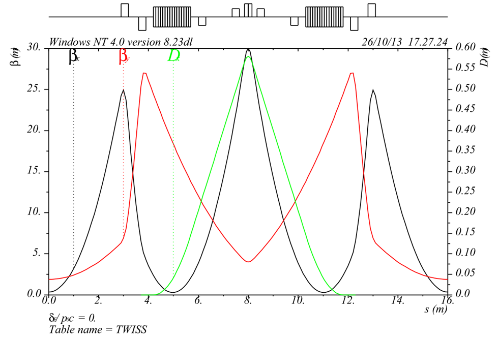
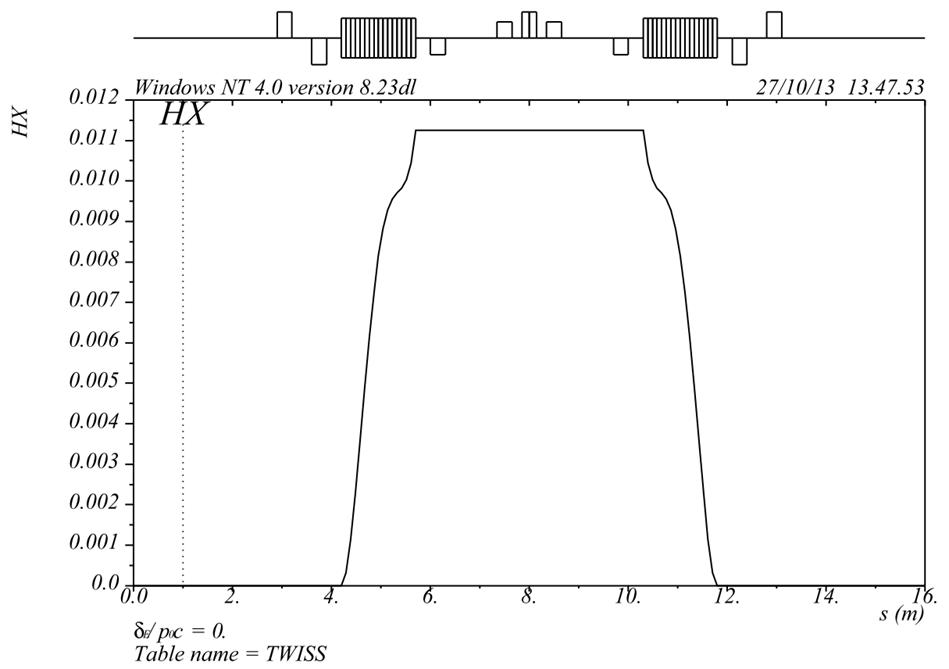
Figure 9: Lattice functions in a DBA cell. Top: Courant–Snyder parameters and dispersion. Bottom: $\mathcal{H}$ function. The horizontal beta and alpha functions at the entrance of the first dipole have values $\beta_{x}=2.08\,$m and $\alpha_{x}=2.47$. These are different from the ‘ideal’ values for low emittance in this case, of $\beta_{x}=2.33\,$m and $\alpha_{x}=3.87$. The lattice functions are detuned from their ideal values in order to satisfy a range of constraints (such as maximum values of the beta functions, magnet strengths and chromaticity). The detuning results in this case in an increase in the natural emittance by a factor of 1.8.

To complete the DBA cell, we need to include some additional quadrupoles in the zero-dispersion region to control the horizontal and vertical beta functions. To correct the chromaticity, sextupoles are included between the dipoles, where the dispersion is non-zero. The lattice functions in an example DBA cell are shown in Fig. 9. To get some idea whether this style of lattice likely to have a lower natural emittance than a FODO lattice, we can inspect the $\mathcal{H}$ function. Comparing Figs. 7 and 9, we see that the $\mathcal{H}$ function is much smaller in the DBA lattice than in the FODO lattice. Note that we use the same dipoles (bending angle and length) in both cases.

Let us calculate the minimum natural emittance of a DBA lattice, for given bending radius $\rho$ and bending angle $\theta$ in the dipoles. To do this, we need to calculate the minimum value of:

$$I_{5}=\int_{0}^{L}\frac{\mathcal{H}_{x}}{\rho^{3}}\,ds$$ (159)

in one dipole (of length $L$), subject to the constraints:

$$\eta_{x,0}=\eta_{px,0}=0,$$ (160)

where $\eta_{x,0}$ and $\eta_{px,0}$ are the dispersion and gradient of the dispersion at the entrance of the dipole. We know how the dispersion and the Courant–Snyder parameters evolve through the dipole, so we can calculate $I_{5}$ for one dipole, for given initial values of the Courant–Snyder parameters $\alpha_{x,0}$ and $\beta_{x,0}$. Then, we have to minimise the value of $I_{5}$ with respect to $\alpha_{x,0}$ and $\beta_{x,0}$. Again, the algebra is rather formidable, and the full expression for $I_{5}$ is not especially enlightening: therefore, we just quote the significant results. We find that, for given $\rho$ and $\theta$ and with the constraints (160) the minimum value of $I_{5}$ is given by:

$$I_{5,\textrm{min}}=\frac{1}{4\sqrt{15}}\frac{\theta^{4}}{\rho}+O(\theta^{6}).$$ (161)

This minimum occurs for values of the Courant–Snyder parameters at the entrance to the dipole given by:

$$\beta_{x,0} = \sqrt{\frac{12}{5}}L+O(\theta^{3}),$$ (162)

$$\alpha_{x,0} = \sqrt{15}+O(\theta^{2}),$$ (163)

where $L=\rho\theta$ is the length of a dipole. Since we know that $I_{2}$ in a single dipole is given by:

$$I_{2}=\int_{0}^{L}\frac{1}{\rho^{2}}\,ds=\frac{\theta}{\rho},$$ (164)

we can now write down an expression for the minimum emittance in a DBA lattice:

$$\varepsilon_{0,\textrm{DBA,min}}=C_{q}\gamma^{2}\frac{I_{5,\textrm{min}}}{j_{x}I_{2}}\approx\frac{1}{4\sqrt{15}}C_{q}\gamma^{2}\theta^{3}.$$ (165)

The approximation is valid for small $\theta$. Note that we have again assumed that, since there is no quadrupole component in the dipole, $j_{x}\approx 1$.

Compare the expression (165) for the minimum emittance in a DBA lattice, with the expression (154) for the minimum emittance in a FODO lattice. We see that in both cases (FODO and DBA), the emittance scales with the square of the beam energy, and with the cube of the bending angle. However, the emittance in a DBA lattice is smaller than that in a FODO lattice (for given energy and dipole bending angle) by a factor $4\sqrt{15}\approx 15.5$.

This is a significant improvement; however, there is still the possibility of reducing the natural emittance (for a given beam energy and number of cells) even further. For a DBA lattice, we imposed constraints (160) on the dispersion at the entrance of the first dipole in a lattice cell. To reach a lower emittance, we can consider relaxing these constraints.

3.3 Theoretical minimum emittance lattice

To derive the conditions for a theoretical minimum emittance (TME) lattice, we write down an expression for:

$$I_{5}=\int_{0}^{L}\frac{\mathcal{H}_{x}}{\rho}\,ds,$$ (166)

with arbitrary dispersion $\eta_{x,0}$, $\eta_{px,0}$ and Courant–Snyder parameters $\alpha_{x,0}$ and $\beta_{x,0}$ in a dipole with given bending radius $\rho$ and angle $\theta$ (and length $L=\rho\theta$). Then, we minimise $I_{5}$ with respect to $\eta_{x,0}$, $\eta_{px,0}$, $\alpha_{x,0}$ and $\beta_{x,0}$. The result is [11]:

$$\varepsilon_{0,\textrm{TME,min}}\approx\frac{1}{12\sqrt{15}}C_{q}\gamma^{2}\theta^{3}.$$ (167)

The minimum emittance is obtained with dispersion at the entrance to the dipole given by:

$$\eta_{x,0} = \frac{1}{6}L\theta+O(\theta^{3}),$$ (168)

$$\eta_{px,0} = -\frac{\theta}{2}+O(\theta^{3}),$$ (169)

and with Courant–Snyder functions at the entrance:

$$\beta_{x,0} = \frac{8}{\sqrt{15}}L+O(\theta^{2}),$$ (170)

$$\alpha_{x,0} = \sqrt{15}+O(\theta^{2}).$$ (171)

The dispersion and beta function reach minimum values in the centre of the dipole:

$$\eta_{x,\textrm{min}} = \rho\left(1-\frac{2}{\theta}\sin\!\left(\frac{\theta}{2}\right)\right)=\frac{L\theta}{24}+O(\theta^{4}),$$ (172)

$$\beta_{x,\textrm{min}} = \frac{L}{2\sqrt{15}}+O(\theta^{2}).$$ (173)

By symmetry, we can consider a single TME cell to contain a single dipole, rather than a pair of dipoles as was necessary for the DBA cell. Outside the dipole, the dispersion is relatively large. This is not ideal for a light source, since insertion devices at locations with large dispersion will blow up the emittance. If insertion devices are required, then it is possible to break the symmetry of the lattice to include zero-dispersion straights: for example, the ring could have a race-track footprint, with arcs constructed from TME cells.

Examples of the lattice functions (and $\mathcal{H}$ function) in a TME cell are shown in Fig. 10. Note that the $\mathcal{H}$ function in the dipole in the TME cell is significantly lower than for FODO or DBA cells using similar dipoles (Figs. 7 and 9).

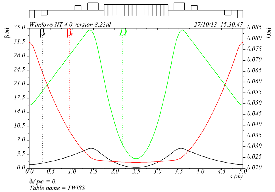
Figure 10: Lattice functions in a TME cell. Top: Courant–Snyder parameters and dispersion. Bottom: $\mathcal{H}$ function. The horizontal beta function and dispersion match the ‘ideal’ values for low emittance.

3.4 Practical constraints on lattice optics

The results we have derived for the natural emittance in FODO, DBA and TME lattices have been for ‘ideal’ lattices that perfectly achieve the stated conditions in each case. In practice, lattices rarely, if ever, achieve the ideal conditions. In particular, the beta function in an achromat is usually not optimal for low emittance; and it is difficult to tune the dispersion for the ideal TME conditions. The main reasons for this are: first, beam dynamics issues (relating, for example, to nonlinear dynamics and collective effects) often impose a variety of strong constraints on the design; and second, optimising the lattice functions while respecting all the various constraints can require complex configurations of quadrupoles. A particularly challenging constraint on design of a low-emittance lattice is the dynamic aperture. Storage rings require a large dynamic aperture in order to achieve good injection efficiency and good beam lifetime. However, low emittance lattices generally need low dispersion and beta functions, and hence require strong quadrupoles. As a result, the chromaticity can be large, and must be corrected using strong sextupoles. Strong sextupoles lead to highly nonlinear motion and a limited dynamic aperture: the trajectories of particles at even quite modest betatron amplitudes or energy deviations can become unstable, resulting in short beam lifetime.

Lattices composed of DBA cells have been a popular choice for third generation synchrotron light sources. The DBA structure provides a lower natural emittance than a FODO lattice with the same number of dipoles, while the long, dispersion-free straight sections provide ideal locations for insertion devices such as undulators and wigglers. If an insertion device, such as an undulator or wiggler, is incorporated in a storage ring at a location with large dispersion, then the dipole fields in the device can make a significant contribution to the quantum excitation ($I_{5}$). As a result, the insertion device can lead to an increase in the natural emittance of the storage ring. By using a DBA lattice, dispersion-free straights are naturally provided, in which undulators and wigglers can be located without blowing up the natural emittance. However, there is some tolerance. In many cases, it is possible to detune the lattice from the strict DBA conditions, thereby allowing some reduction in natural emittance at the cost of some dispersion in the straights. The insertion devices will then contribute to the quantum excitation; but depending on the lattice and the insertion devices, there may still be a net benefit. Some light sources that were originally designed with zero-dispersion straights take advantage of tuning flexibility to operate with non-zero dispersion in the straights (see, for example, [12]). This provides a lower natural emittance, and better output for users.

3.5 Multi-bend achromats

There are of course many options for the design of a storage ring lattice, beyond the FODO, DBA and TME cells we have discussed so far. For example, it is possible to combine the DBA and TME lattices, constructing an arc cell consisting of more than two dipoles. The dipoles at either end of the cell have zero dispersion (and gradient of the dispersion) at their outside faces, thus satisfying the achromat condition. Since the lattice functions are different in the central dipoles compared to the end dipoles, we have additional degrees of freedom we can use to minimise the quantum excitation. The result is a multi-bend achromat (MBA) that combines the benefits of a DBA lattice (with long straights providing good locations for insertion devices) and a TME lattice (providing the possibility of achieving lower emittance than in a DBA).

In a MBA, it is possible to have cases where the end dipoles and central dipoles differ in the bend angle (i.e. length of dipole), and/or the bend radius (i.e. strength of dipole). For simplicity, let us consider the case where the dipoles all have the same bending radius (i.e. they all have the same field strength), but they vary in length. Assume that each arc cell has a fixed number $M$ of dipoles, with average bending angle $\theta=2\pi/MN_{\textrm{cells}}$. If the two outer dipoles have bending angle $a\theta$ and the inner dipoles have bending angle $b\theta$, then the coefficients $a$ and $b$ satisfy:

$$2a+(M-2)b=M.$$ (174)

Let us assume that the lattice functions (Courant–Snyder parameters and dispersion) in the outer dipoles are the same as in a DBA lattice, and in the inner dipoles are the same as in a TME lattice. Since the synchrotron radiation integrals are additive, for an $M$-bend achromat, we can write:

$$I_{5,\textrm{cell}} \approx \frac{2}{4\sqrt{15}}\frac{(a\theta)^{4}}{\rho}+\frac{(M-2)}{12\sqrt{15}}\frac{(b\theta)^{4}}{\rho}=\frac{6a^{4}+(M-2)b^{4}}{12\sqrt{15}}\frac{\theta^{4}}{\rho},$$ (175)

$$I_{2,\textrm{cell}} \approx 2\frac{a\theta}{\rho}+(M-2)\frac{b\theta}{\rho}=\left(2a+(M-2)b\right)\frac{\theta}{\rho}.$$ (176)

Hence, in an $M$-bend achromat:

$$\frac{I_{5,\textrm{cell}}}{I_{2,\textrm{cell}}}\approx\frac{1}{12\sqrt{15}}\left(\frac{6a^{4}+(M-2)b^{4}}{2a+(M-2)b}\right)\theta^{3}.$$ (177)

Minimising the ratio $I_{5}/I_{2}$ with respect to $a$ gives:

$$\frac{a}{b}=\frac{1}{\sqrt[3]{3}},$$ (178)

from which it follows that:

$$\left(\frac{6a^{4}+(M-2)b^{4}}{2a+(M-2)b}\right)\approx\frac{M+1}{M-1}.$$ (179)

The central bending magnets should be longer than the outer bending magnets by a factor $\sqrt[3]{3}$. Then, the minimum natural emittance in an $M$-bend achromat is given by:

$$\varepsilon_{0,\textrm{MBA,min}}\approx\frac{1}{12\sqrt{15}}\left(\frac{M+1}{M-1}\right)C_{q}\gamma^{2}\theta^{3}.$$ (180)

Note that $\theta$ is the average bending angle per dipole. Although we derived (180) with the assumption of at least three dipoles ($M>2$), the formula gives the correct result for a DBA in the case $M=2$. Also, in the limit $M\to\infty$, we obtain the correct expression for the natural emittance in a TME lattice.

Triple bend achromats have been used in light sources, including the ALS [13] and the SLS [14]. Light sources based on cells with even larger numbers of bends per achromat are planned: see, for example, [15]. As with double bend achromats, it is possible to obtain some reduction in the natural emittance of a triple (or higher) bend achromat by detuning the lattice from the strict achromat condition, allowing some dispersion to ‘leak’ into the straight sections. As long as the dispersion in the straights is not too large, there is a net benefit, despite some contribution to the emittance from quantum excitation in the insertion devices.

As a final remark, we note that further flexibility to optimise the natural emittance can be provided by relaxing the constraint that the field strength in a dipole is constant along the length of the dipole. We expect an optimised design to have the strongest field at the centre of the dipole, where the dispersion can be minimised. For an example, see [16].

Table 1: Minimum natural emittance in different lattice styles for electron storage rings: for each lattice style, the minimum natural emittance is given by $\mathcal{F}C_{q}\gamma^{2}\theta^{3}$, where $C_{q}\approx 3.832\times 10^{-13}\,$m, and $\gamma$ is the relativistic factor for the beam. The dipoles have length $L$ and bending angle $\theta$, and no quadrupole component.

Lattice style	$\mathcal{F}$	Conditions
90∘ FODO	$2\sqrt{2}$	$f=L/\sqrt{2}$
137∘ FODO	$1.2$	minimum emittance FODO
DBA	$\frac{1}{4\sqrt{15}}$	$\eta_{x,0}=\eta_{px,0}=0,\quad\beta_{x,0}\approx\sqrt{12/5}L\quad\alpha_{x,0}\approx\sqrt{15}$
MBA	$\frac{1}{12\sqrt{15}}\left(\frac{M+1}{M-1}\right)$	$M$ dipoles (with same radius of curvature) per cell
TME	$\frac{1}{12\sqrt{15}}$	$\eta_{x,\textrm{min}}\approx\frac{L\theta}{24}\quad\beta_{x,\textrm{min}}\approx\frac{L}{2\sqrt{15}}$

4 Vertical emittance generation, calculation and tuning

In this section, we shall discuss how vertical emittance is generated by alignment and tuning errors, describe methods for calculating the vertical emittance in the presence of known errors, and discuss briefly how an operating storage ring can be tuned to minimise the vertical emittance (even when the alignment and tuning errors are not well known).

Recall that the natural (horizontal) emittance in a storage ring is given by (108):

$$\varepsilon_{0}=C_{q}\gamma^{2}\frac{I_{5}}{j_{x}I_{2}}.$$ (181)

If the horizontal and vertical motion are independent of each other (i.e. if there is no betatron coupling) then we can apply the same analysis to the vertical motion as we did to the horizontal. If we build a ring that is completely flat (i.e. no vertical bending), then there is no vertical dispersion, i.e. $\eta_{y}=\eta_{py}=0$ at all locations around the ring. It follows that the vertical $\mathcal{H}$ function $\mathcal{H}_{y}$:

$$\mathcal{H}_{y}=\gamma_{y}\eta_{y}^{2}+2\alpha_{y}\eta_{y}\eta_{py}+\beta_{y}\eta_{py}^{2},$$ (182)

also vanishes around the entire ring, and that therefore the synchrotron radiation integral $I_{5y}$ will be zero. This implies that the vertical emittance will damp to zero.

However, in deriving equation (181) for the natural emittance, we assumed that all photons were emitted directly along the instantaneous direction of motion of the electron. In fact, photons are emitted with a distribution having angular width $1/\gamma$ about the direction of motion of the electron. This leads to some vertical ‘recoil’ that excites vertical betatron motion, resulting in a non-zero vertical emittance. A detailed analysis leads to the following formula for the fundamental lower limit on the vertical emittance [9]:

$$\varepsilon_{y,\textrm{min}}=\frac{13}{55}\frac{C_{q}}{j_{y}I_{2}}\oint\frac{\beta_{y}}{|\rho|^{3}}\,ds.$$ (183)

To estimate a typical value for the lower limit on the vertical emittance, let us write equation (183) in the approximate form:

$$\varepsilon_{y,\textrm{min}}\approx\frac{C_{q}\langle\beta_{y}\rangle}{4j_{y}I_{2}}\oint\frac{1}{|\rho|^{3}}\,ds=\frac{\langle\beta_{y}\rangle}{4}\frac{j_{z}}{j_{y}}\frac{\sigma_{\delta}^{2}}{\gamma^{2}},$$ (184)

where $\langle\beta_{y}\rangle$ is the average vertical beta function around the ring. Using some typical values ($\langle\beta_{y}\rangle=20$ m, $j_{z}=2$, $j_{y}=1$, $\sigma_{\delta}=10^{-3}$, $\gamma=6000$), we find:

$$\varepsilon_{y,\textrm{min}}\approx 0.3\,\textrm{pm}.$$ (185)

The lowest vertical emittance achieved so far in a storage ring is around a picometer, several times larger than the fundamental lower limit (see, for example, [17, 18]). In practice, vertical emittance in a (nominally planar) storage ring is dominated by two effects: residual vertical dispersion, which couples longitudinal and vertical motion; and betatron coupling, which couples horizontal and vertical motion. The dominant causes of residual vertical dispersion and betatron coupling are magnet alignment errors, in particular: tilts of the dipoles around the beam axis; vertical alignment errors on the quadrupoles; tilts of the quadrupoles around the beam axis; and vertical alignment errors of the sextupoles. Let us consider these errors in a little more detail.

Steering errors lead to a distortion of the closed orbit, which generates vertical dispersion and (through vertical offsets of the beam in the sextupoles) betatron coupling. A vertical steering error may be generated by rotation of a dipole, so that the field is not exactly vertical, or by vertical misalignment of a quadrupole, so that there is a horizontal magnetic field at the location of the reference trajectory.

Coupling errors lead to a transfer of horizontal betatron motion and dispersion into the vertical plane: in both cases, the result is an increase in vertical emittance. Coupling may result from rotation of a quadrupole, so that the field contains a skew component. When particles pass through a skew quadrupole, they receive a vertical kick that depends on their horizontal offset. As a result, quantum excitation of the horizontal emittance feeds into the vertical plane.

A vertical beam offset in a sextupole has the same effect as a skew quadrupole. To understand this, recall that a sextupole field is given by:

$$B_{x} = (B\rho)k_{2}xy,$$ (186)

$$B_{y} = \frac{1}{2}(B\rho)k_{2}\left(x^{2}-y^{2}\right).$$ (187)

A vertical offset can be represented by the transformation $y\mapsto y+\Delta y$:

$$B_{x} \mapsto (B\rho)k_{2}xy+(B\rho)k_{2}\Delta y\,x,$$ (188)

$$B_{y} \mapsto \frac{1}{2}(B\rho)k_{2}\left(x^{2}-y^{2}\right)-(B\rho)k_{2}\Delta y\,y-\frac{1}{2}k_{2}\Delta y^{2}.$$ (189)

The terms in (188) and (189) that are first order in $\Delta y$ constitute a skew quadrupole of strength $(B\rho)k_{2}\Delta y$.

When designing and building a storage ring, we need to know how accurately the magnets must be aligned, to keep the vertical emittance below some specified limit. Although beam-based tuning methods also normally have to be applied, the ultimate emittance achieved after machine tuning does depend on the accuracy with which the initial alignment is performed. It is therefore useful to have expressions that relate the closed orbit distortion, vertical dispersion, betatron coupling and (ultimately) the vertical emittance, to the alignment errors on the magnets.

4.1 Closed orbit distortion

Let us begin by considering the closed orbit distortion. In terms of the action-angle variables, we can write the coordinate and momentum of a particle at any point:

$$y = \sqrt{2\beta_{y}J_{y}}\cos\phi_{y},$$ (190)

$$p_{y} = -\sqrt{\frac{2J_{y}}{\beta_{y}}}\left(\sin\phi_{y}+\alpha_{y}\cos\phi_{y}\right).$$ (191)

Suppose there is a steering error at some location $s=s_{0}$ which leads to an instantaneous change (i.e. a ‘kick’) $\Delta\theta$ in the vertical momentum. After one complete turn of the storage ring, starting from immediately after $s_{0}$, the trajectory of a particle will close on itself if:

$$\sqrt{2\beta_{y0}J_{y0}}\cos\phi_{y1} = \sqrt{2\beta_{y0}J_{y0}}\cos\phi_{y0},$$ (192)

$$-\sqrt{\frac{2J_{y0}}{\beta_{y0}}}\left(\sin\phi_{y1}+\alpha_{y0}\cos\phi_{y1}\right) = -\sqrt{\frac{2J_{y0}}{\beta_{y0}}}\left(\sin\phi_{y0}+\alpha_{y0}\cos\phi_{y0}\right)-\Delta\theta.$$

where $\phi_{y1}=\phi_{y0}+2\pi\nu_{y}$, and $\nu_{y}=\mu_{y}/2\pi$ is the vertical tune (see Fig. 11). Solving equations (192) and (LABEL:codpy) for the action and angle at $s_{0}$:

$$J_{y0} = \frac{\beta_{y0}\Delta\theta^{2}}{8\sin^{2}\pi\nu_{y}},$$ (194)

$$\phi_{y0} = \pi\nu_{y}.$$ (195)

Note that if the tune is an integer, there is no solution for the closed orbit: even the smallest steering error will kick the beam out of the ring. From (195), we can write the coordinate for the closed orbit at any point in the ring:

$$y_{\mathrm{co}}(s)=\frac{\sqrt{\beta_{y}(s_{0})\beta_{y}(s)}}{2\sin\pi\nu_{y}}\Delta\theta\cos\!\left(\pi\nu_{y}+\mu_{y}(s;s_{0})\right),$$ (196)

where $\mu_{y}(s;s_{0})$ is the phase advance from $s_{0}$ to $s$.

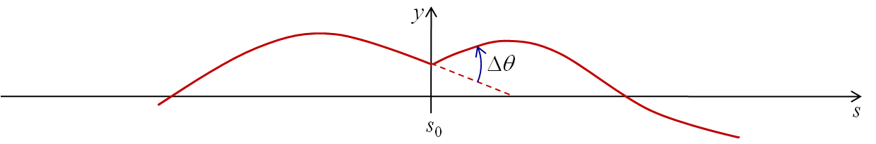
Figure 11: Closed orbit distortion from a thin dipole kick in a synchrotron storage ring. If the co-ordinate and momentum of a particle on the closed orbit immediately after the dipole kick are $(y_{0},p_{y0})$, then after nearly one complete turn, just before the dipole kick the co-ordinate and momentum of the particle are $(y_{0},p_{y0}-\Delta\theta)$. The dipole kick then puts the particle back onto the closed orbit.

In general, there will be many steering errors distributed around a storage ring. The closed orbit can be found by summing the effects of all the steering errors:

$$y_{\mathrm{co}}(s)=\frac{\sqrt{\beta_{y}(s)}}{2\sin\pi\nu_{y}}\oint\sqrt{\beta_{y}(s^{\prime}})\frac{d\theta}{ds^{\prime}}\cos\!\left(\pi\nu_{y}+\mu_{y}(s;s^{\prime})\right)\,ds^{\prime}.$$ (197)

It is often helpful to be able to estimate the size of the closed orbit distortion that may be expected from random quadrupole misalignments of a given magnitude. We can derive an expression for this from equation (197). For a quadrupole of integrated focusing strength $k_{1}L$, vertically misaligned from the reference trajectory by $\Delta Y$, the steering is:

$$\Delta\theta=(k_{1}L)\Delta Y.$$ (198)

Squaring equation (197), then averaging over many seeds of random alignment errors, we find:

$$\left\langle\frac{y_{\mathrm{co}}^{2}(s)}{\beta_{y}(s)}\right\rangle=\frac{\langle\Delta Y^{2}\rangle}{8\sin^{2}\pi\nu_{y}}\sum_{\textrm{quads}}\beta_{y}(k_{1}L)^{2}.$$ (199)

In performing the average, we assume that the alignments of different quadrupoles are not correlated in any way.

The ratio between the closed orbit rms and the magnet misalignment rms is sometimes known as the orbit amplification factor. Values for the orbit amplification factor are typically in the range from 10 to about 100. Of course, the amplification factor is a statistical quantity: the actual rms of the orbit distortion depends on the particular set of alignment errors present.

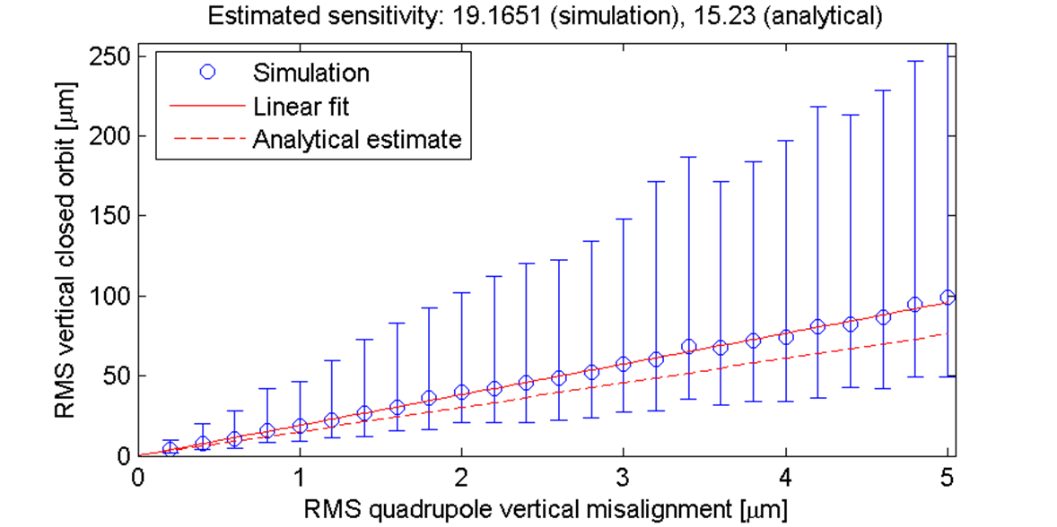
Figure 12: Simulation of closed orbit distortion resulting from quadrupole alignment errors in a storage ring [19]. Each circle shows the mean of the rms orbit distortion from 100 different sets (seeds) of random alignment errors on the quadrupoles; the error bars show the range covered by 90% of the seeds. The solid red line shows a linear fit to the circles; the broken red line shows an analytical estimate of the orbit distortion based on the known quadrupole strengths and lattice functions, using equation (199).

In the context of low-emittance storage rings, vertical closed orbit errors are of concern for two reasons. First, vertical steering generates vertical dispersion, which is a source of vertical emittance. Second, vertical orbit errors contribute to vertical beam offset in the sextupoles, which effectively generates skew quadrupole fields, which in turn lead to betatron coupling. We have seen how to analyse the beam dynamics to understand the closed orbit distortion that arises from quadrupole alignment errors of a given magnitude. Our goal is to relate quantities such as orbit distortion, vertical dispersion, coupling, and vertical emittance, to the alignment errors on the magnets. We continue with betatron coupling.

4.2 Betatron coupling

Betatron coupling describes the effects that can arise when the vertical motion of a particle depends on its horizontal motion, and vice-versa. Betatron coupling can arise (for example) from skew quadrupoles and solenoids.

In a storage ring, skew quadrupole fields ofen arise from quadrupole tilts, and from vertical alignment errors on sextupoles. A full treatment of betatron coupling can become quite complex, and there are many different formalisms that can be used. However, it is possible to use a simplified model to derive approximate expressions the equilibrium emittances in the presence of coupling. The procedure is as follows. First, we write down the equations of motion for a single particle in a beamline containing coupling. Then, we look for a ‘steady state’ solution to the equations of motion, in which the horizontal and vertical actions are each constants of the motion. Finally, we assume that the actions in the steady state solution correspond to the equilibrium emittances (since $\varepsilon=\langle J\rangle$), and that the sum of the horizontal and vertical emittances is equal to the natural emittance of the ‘ideal’ lattice (i.e. the natural emittance of the lattice in the absence of errors). This procedure can give some useful results, but because of the approximations involved, the formulae are not always very accurate.

We will use Hamiltonian mechanics. In this formalism, the equations of motion for the action-angle variables (with path length $s$ as the independent variable) are derived from the Hamiltonian:

$$H=H(\phi_{x},J_{x},\phi_{y},J_{y};s),$$ (200)

using Hamilton’s equations:

$$\frac{dJ_{x}}{ds} = -\frac{\partial H}{\partial\phi_{x}},$$ (201)

$$\frac{dJ_{y}}{ds} = -\frac{\partial H}{\partial\phi_{y}},$$ (202)

$$\frac{d\phi_{x}}{ds} = \frac{\partial H}{\partial J_{x}},$$ (203)

$$\frac{d\phi_{y}}{ds} = \frac{\partial H}{\partial J_{y}}.$$ (204)

For a particle moving along a linear, uncoupled beamline, the Hamiltonian is:

$$H=\frac{J_{x}}{\beta_{x}}+\frac{J_{y}}{\beta_{y}}.$$ (205)

The first step is to derive an appropriate form for the Hamiltonian in a storage ring with skew quadrupole perturbations. In Cartesian variables, the equations of motion in a skew quadrupole can be written:

$$\frac{dp_{x}}{ds} = k_{s}y,$$ (206)

$$\frac{dp_{y}}{ds} = k_{s}x,$$ (207)

$$\frac{dx}{ds} = p_{x},$$ (208)

$$\frac{dy}{ds} = p_{y},$$ (209)

where:

$$k_{s}=\frac{1}{B\rho}\frac{\partial B_{x}}{\partial x}.$$ (210)

These equations can be derived from the Hamiltonian:

$$H=\frac{1}{2}p_{x}^{2}+\frac{1}{2}p_{y}^{2}-k_{s}xy.$$ (211)

We are interested in the case where there are skew quadrupoles distributed around a storage ring. The ‘focusing’ effect of a skew quadrupole is represented by a term in the Hamiltonian:

$$k_{s}xy=2k_{s}\sqrt{\beta_{x}\beta_{y}}\sqrt{J_{x}J_{y}}\cos\phi_{x}\cos\phi_{y}.$$ (212)

This implies that the Hamiltonian for a beam line with distributed skew quadrupoles can be written:

$$H=\frac{J_{x}}{\beta_{x}}+\frac{J_{y}}{\beta_{y}}-2k_{s}(s)\sqrt{\beta_{x}\beta_{y}}\sqrt{J_{x}J_{y}}\cos\phi_{x}\cos\phi_{y}.$$ (213)

The beta functions and the skew quadrupole strength are functions of the position $s$. This makes it difficult to solve the equations of motion exactly. Therefore, we simplify the problem by ‘averaging’ the Hamiltonian:

$$H=\omega_{x}J_{x}+\omega_{y}J_{y}-2\bar{\kappa}\sqrt{J_{x}J_{y}}\cos\phi_{x}\cos\phi_{y}.$$ (214)

Here, $\omega_{x}$, $\omega_{y}$ are the phase advances per unit length of the beam line, given by:

$$\omega_{x,y}=\frac{1}{C_{0}}\int_{0}^{C_{0}}\frac{ds}{\beta_{x,y}},$$ (215)

where $C_{0}$ is the circumference of the ring. $\bar{\kappa}$ is a constant that characterises the coupling strength. For reasons that will become clear shortly, we re-write the coupling term, to put the Hamiltonian in the form:

$$H=\omega_{x}J_{x}+\omega_{y}J_{y}-\bar{\kappa}_{-}\sqrt{J_{x}J_{y}}\cos(\phi_{x}-\phi_{y})-\bar{\kappa}_{+}\sqrt{J_{x}J_{y}}\cos(\phi_{x}+\phi_{y}).$$ (216)

The constants $\bar{\kappa}_{\pm}$ represent the skew quadrupole strength averaged around the ring. However, we need to take into account that the kick from a skew quadrupole depends on the betatron phase. Thus, we write:

$$\bar{\kappa}_{\pm}e^{i\chi}=\frac{1}{C_{0}}\int_{0}^{C_{0}}e^{i(\mu_{x}\pm\mu_{y})}k_{s}\sqrt{\beta_{x}\beta_{y}}\,ds,$$ (217)

where $\mu_{x}$ and $\mu_{y}$ are the betatron phase advances from the start of the ring.

Now suppose that $\bar{\kappa}_{-}\gg\bar{\kappa}_{+}$. (This can occur, for example, if $\omega_{x}\approx\omega_{y}$, in which case all the contributions to $\bar{\kappa}_{-}$ from the skew quadrupole perturbations will add together in phase.) Then, we can simplify things further by dropping the term in $\bar{\kappa}_{+}$ from the Hamiltonian:

$$H=\omega_{x}J_{x}+\omega_{y}J_{y}-\bar{\kappa}_{-}\sqrt{J_{x}J_{y}}\cos(\phi_{x}-\phi_{y}).$$ (218)

We can now write down the equations of motion:

$$\frac{dJ_{x}}{ds} = -\frac{\partial H}{\partial\phi_{x}}=\bar{\kappa}_{-}\sqrt{J_{x}J_{y}}\sin(\phi_{x}-\phi_{y}),$$ (219)

$$\frac{dJ_{y}}{ds} = -\frac{\partial H}{\partial\phi_{y}}=-\bar{\kappa}_{-}\sqrt{J_{x}J_{y}}\sin(\phi_{x}-\phi_{y}),$$ (220)

$$\frac{d\phi_{x}}{ds} = \frac{\partial H}{\partial J_{x}}=\omega_{x}+\frac{\bar{\kappa}_{-}}{2}\sqrt{\frac{J_{x}}{J_{y}}}\cos(\phi_{x}-\phi_{y}),$$ (221)

$$\frac{d\phi_{y}}{ds} = \frac{\partial H}{\partial J_{y}}=\omega_{y}+\frac{\bar{\kappa}_{-}}{2}\sqrt{\frac{J_{y}}{J_{x}}}\cos(\phi_{x}-\phi_{y}).$$ (222)

Even after all the simplifications we have made, the equations of motion are still rather difficult to solve. Fortunately, however, we do not require the general solution. In fact, we are only interested in the properties of some special cases. First of all, we note that from (219) and (220):

$$\frac{dJ_{x}}{ds}+\frac{dJ_{y}}{ds}=0,$$ (223)

and therefore the sum of the actions $J_{x}+J_{y}$ is constant. Going further, we notice that if $\phi_{x}=\phi_{y}$, then the rate of change of each action falls to zero. This implies that if we can find a solution to the equations of motion with $\phi_{x}=\phi_{y}$ for all $s$, then the actions will remain constant. In fact, we find that if $\phi_{x}=\phi_{y}$, and:

$$\frac{d\phi_{x}}{ds}=\frac{d\phi_{y}}{ds},$$ (224)

then:

$$\frac{J_{y}}{J_{x}}=\frac{\sqrt{1+\bar{\kappa}_{-}^{2}/\Delta\omega^{2}}-1}{\sqrt{1+\bar{\kappa}_{-}^{2}/\Delta\omega^{2}}+1},$$ (225)

where $\Delta\omega=\omega_{x}-\omega_{y}$. If we further use $J_{x}+J_{y}=J_{0}$, where $J_{0}$ is a constant, then we have a solution to the equations of motion in which the actions are constant, and given by:

$$J_{x} = \frac{1}{2}\left(1+\frac{1}{\sqrt{1+\bar{\kappa}_{-}^{2}/\Delta\omega^{2}}}\right)J_{0},$$ (226)

$$J_{y} = \frac{1}{2}\left(1-\frac{1}{\sqrt{1+\bar{\kappa}_{-}^{2}/\Delta\omega^{2}}}\right)J_{0}.$$ (227)

Note the behaviour, shown in Fig. 13, of the fixed actions as we vary the ‘coupling strength’ $\bar{\kappa}_{-}$ and the betatron tunes (betatron frequencies). The fixed actions are well-separated for $\bar{\kappa}_{-}\ll\Delta\omega$, but both approach the value $J_{0}/2$ for $\bar{\kappa}_{-}\gg\Delta\omega$. The condition at which the tunes are equal (or differ by an exact integer) is known as the difference coupling resonance.

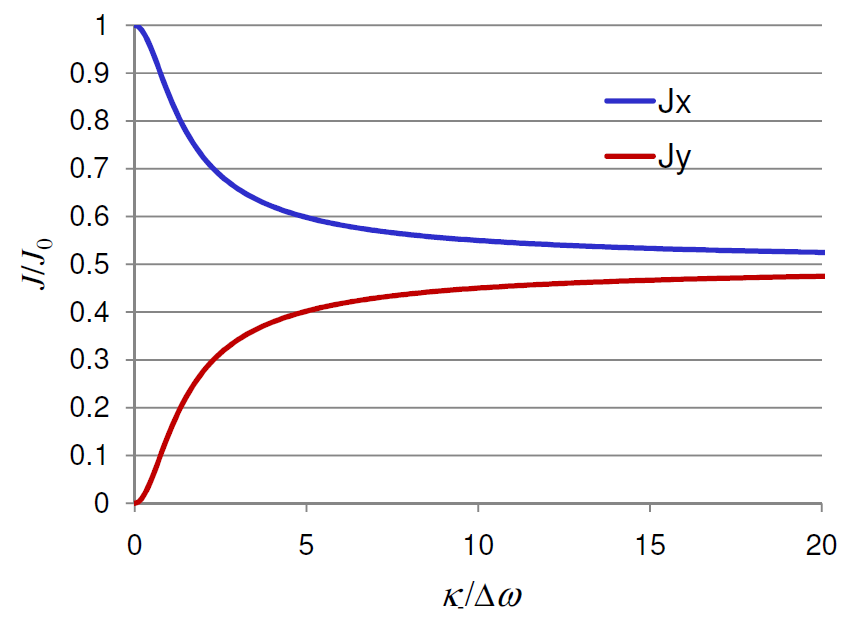
Figure 13: Variation of the ‘fixed point’ actions (226) and (227) as a function of the strength of the coupling resonance.

Recall that the emittance may be defined as the betatron action averaged over all particles in the beam:

$$\varepsilon_{x}=\langle J_{x}\rangle,\qquad\textrm{and}\qquad\varepsilon_{y}=\langle J_{y}\rangle.$$ (228)

Now, synchrotron radiation will damp the beam towards an equilibrium distribution. In this equilibrium, we expect the betatron actions of the particles to change only slowly, i.e. on the timescale of the radiation damping, which is much longer than the timescale of the betatron motion. In that case, the actions of most particles must be in the correct ratio for a fixed-point solution to the equations of motion. Then, if we assume that $\varepsilon_{x}+\varepsilon_{y}=\varepsilon_{0}$, where $\varepsilon_{0}$ is the natural emittance of the storage ring, we must have for the equilibrium emittances:

$$\varepsilon_{x} = \left(1+\frac{1}{\sqrt{1+\bar{\kappa}_{-}^{2}/\Delta\omega^{2}}}\right)\frac{\varepsilon_{0}}{2},$$ (229)

$$\varepsilon_{y} = \left(1-\frac{1}{\sqrt{1+\bar{\kappa}_{-}^{2}/\Delta\omega^{2}}}\right)\frac{\varepsilon_{0}}{2}.$$ (230)

As an illustration, we can plot the vertical emittance as a function of the ‘tune split’ $\Delta\nu$, in a model of the ILC damping rings, with a single skew quadrupole (located at a point of zero dispersion, so as not to couple horizontal dispersion into the vertical plane). The result is shown in Fig. 14. The tunes are controlled by adjusting the regular (normal) quadrupoles in the lattice. The simulation results are based on emittance calculation using Chao’s method, which we shall discuss later.

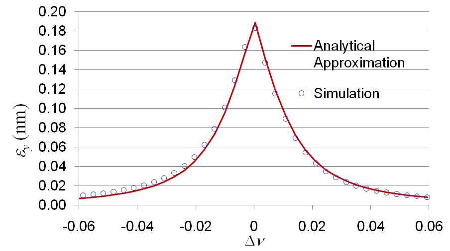
Figure 14: Effect of a single skew quadrupole (at a location with zero dispersion) on the vertical emittance in a synchrotron storage ring, as a function of the difference in the betatron tunes. The circles show the results of a computation using Chao’s method [21]; the red line shows an analytical estimate using equation (230).

The presence of skew quadrupole errors in a storage ring affects the betatron tunes. To estimate the size of the effect, we use the Hamiltonian (218). If we consider a particle close to the fixed point solution, we can assume that $\phi_{x}=\phi_{y}$, so that the Hamiltonian becomes:

$$H=\omega_{x}J_{x}+\omega_{y}J_{y}-\bar{\kappa}_{-}\sqrt{J_{x}J_{y}}.$$ (231)

The normal modes describe motion that is periodic with a single well-defined frequency. In the absence of coupling, the transverse normal modes correspond to motion in just the horizontal or vertical plane. When coupling is present, the normal modes involve a combination of horizontal and vertical motion.

Let us write the Hamiltonian (231) in the form:

$$H=\left(\begin{array}[]{cc}\sqrt{J_{x}}&\sqrt{J_{y}}\end{array}\right)A\left(\begin{array}[]{c}\sqrt{J_{x}}\\ \sqrt{J_{y}}\end{array}\right),$$ (232)

where:

$$A=\left(\begin{array}[]{cc}\omega_{x}&-\frac{1}{2}\bar{\kappa}_{-}\\ -\frac{1}{2}\bar{\kappa}_{-}&\omega_{y}\end{array}\right).$$ (233)

The normal modes can be constructed from the eigenvectors of the matrix $A$, and the frequency of each mode is given by the corresponding eigenvalue. From the eigenvalues of $A$, we find that the normal mode frequencies are:

$$\omega_{\pm}=\frac{1}{2}\left(\omega_{x}+\omega_{y}\pm\sqrt{\bar{\kappa}_{-}^{2}+\Delta\omega^{2}}\right).$$ (234)

Hence, the tunes $\nu_{\pm}$ are given (in terms of the tunes $\nu_{x}$ and $\nu_{y}$ in the absence of errors) by:

$$\nu_{\pm}=\frac{1}{2}\left(\nu_{x}+\nu_{y}\pm\sqrt{\kappa^{2}+\Delta\nu^{2}}\right),$$ (235)

where, from (217), $\kappa=(C_{0}/2\pi)\bar{\kappa}_{-}$ is given by:

$$\kappa e^{i\chi}=\frac{1}{2\pi}\int_{0}^{C_{0}}e^{i(\mu_{x}-\mu_{y})}k_{s}\sqrt{\beta_{x}\beta_{y}}\,ds.$$ (236)

The dependence of the tunes on the coupling strength provides a useful method for measuring the coupling strength $\kappa$ in a real lattice. The procedure is simple: a quadrupole (or combination of quadrupoles) is used to change the tunes, and then the tunes are recorded and plotted as a function of quadrupole strength. The minimum separation between the measured tunes gives the coupling strength. An example (from simulation) is shown in Fig. 15. Of course, this procedure does not identify the source of the coupling, or provide very much information as to an optimal correction (beyond the strength of a skew quadrupole that may be required to achieve the correction, assuming that the skew quadrupole is at the correct phase in the lattice). However, the technique can be useful to characterise the effect of a correction that may need to be applied in several iterations.

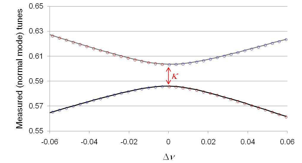
Figure 15: Effect of a single skew quadrupole (at a location with zero dispersion) on the measured betatron tunes in a synchrotron storage ring, as a function of the difference in the betatron tunes in the absence of the skew quadrupole. The circles show the results of a computation of the eigenvalues of the single-turn transfer matrix; the solid lines show an analytical estimate using equation (235). The minimum difference between the measured tunes gives the coupling strength in the ring.

Major sources of coupling in storage rings are quadrupole tilts and sextupole alignment. Using the theory just outlined, we can estimate the alignment tolerances on these magnets, for given optics and specified vertical emittance. Starting with equation (236), we first take the modulus squared, and then use (for a sextupole with vertical alignment error $\Delta Y_{S}$) $k_{s}=k_{2}\Delta Y_{S}$ and (for a quadrupole with tilt error $\Delta\Theta_{Q}$) $k_{s}=k_{1}\Delta\Theta_{Q}$. Assuming that there are no correlations between the errors, we find:

$$\langle\kappa^{2}\rangle\approx\frac{\langle\Delta Y_{S}^{2}\rangle}{4\pi^{2}}\sum_{\mathrm{sexts}}\beta_{x}\beta_{y}(k_{2}l)^{2}+\frac{\langle\Delta\Theta_{Q}^{2}\rangle}{4\pi^{2}}\sum_{\mathrm{quads}}\beta_{x}\beta_{y}(k_{1}l)^{2},$$ (237)

where $\langle\kappa^{2}\rangle$ represents the mean value of the square of the coupling strength over a large number of sets of random errors. Note that $\Delta Y_{S}$ is the beam offset from the centre of a sextupole: this includes the effects of closed orbit distortion.

4.3 Vertical dispersion

Vertical emittance is generated by vertical dispersion as well as by betatron coupling. Vertical dispersion is in turn generated by vertical closed orbit distortion (vertical steering), and coupling of horizontal dispersion into the vertical plane by skew quadrupole fields. Our goal now is to estimate the amount of vertical dispersion generated from magnet alignment errors; we can then estimate the contribution to the vertical emittance.

The equation of motion for the vertical co-ordinate for a particle with momentum $P$ is:

$$\frac{d^{2}y}{ds^{2}}=\frac{B_{x}}{(B\rho)}=\frac{q}{P}B_{x}.$$ (238)

For small energy deviation $\delta$, $P$ is related to the reference momentum $P_{0}$ by:

$$P\approx(1+\delta)P_{0}.$$ (239)

We can write for the horizontal field (to first order in the derivatives):

$$B_{x}\approx B_{0x}+y\frac{\partial B_{x}}{\partial y}+x\frac{\partial B_{x}}{\partial x}.$$ (240)

If we consider a particle following an off-momentum closed orbit, so that:

$$y = \eta_{y}\delta,$$ (241)

$$x = \eta_{x}\delta,$$ (242)

then, combining the above equations, we find to first order in $\delta$:

$$\frac{d^{2}\eta_{y}}{ds^{2}}-k_{1}\eta_{y}\approx-k_{0s}+k_{1s}\eta_{x}.$$ (243)

Equation (243) gives the ‘equation of motion’ for the dispersion. It is similar to the equation of motion for the closed orbit:

$$\frac{d^{2}y_{\mathrm{co}}}{ds^{2}}-k_{1}y_{\mathrm{co}}\approx-k_{0s}+k_{1s}x_{\mathrm{co}}.$$ (244)

We can therefore immediately generalise the relationship (199) between the closed orbit and the quadrupole misalignments, to find for the dispersion:

$$\left\langle\frac{\eta_{y}^{2}}{\beta_{y}}\right\rangle=\frac{\langle\Delta Y_{Q}^{2}\rangle}{8\sin^{2}\pi\nu_{y}}\sum_{\textrm{quads}}\beta_{y}(k_{1}L)^{2}+\frac{\langle\Delta\Theta_{Q}^{2}\rangle}{8\sin^{2}\pi\nu_{y}}\sum_{\textrm{quads}}\eta_{x}^{2}\beta_{y}(k_{1}L)^{2}+\frac{\langle\Delta Y_{S}^{2}\rangle}{8\sin^{2}\pi\nu_{y}}\sum_{\textrm{sexts}}\eta_{x}^{2}\beta_{y}(k_{2}L)^{2}.$$ (245)

Here, we assume that the skew dipole terms $k_{0s}$ come from vertical alignment errors on the quadrupoles with mean square $\langle\Delta Y_{Q}^{2}\rangle$, and that the skew quadrupoles $k_{1s}$ come from tilts on the quadrupoles with mean square $\langle\Delta\Theta_{Q}^{2}\rangle$ and from vertical alignment errors on the sextupoles, with mean square $\langle\Delta Y_{S}^{2}\rangle$. We assume that all alignment errors are uncorrelated.

The final step is to relate the vertical dispersion to the vertical emittance. This is not too difficult. First, we can apply the formula (108) for the natural (horizontal) emittance to the vertical emittance:

$$\varepsilon_{y}=C_{q}\gamma^{2}\frac{I_{5y}}{j_{y}I_{2}},$$ (246)

where $j_{y}$ is the vertical damping partition number (usually, $j_{y}=1$), and the synchrotron radiation integrals are given by:

$$I_{5y}=\oint\frac{\mathcal{H}_{y}}{|\rho|^{3}}\,ds,$$ (247)

and:

$$I_{2}=\oint\frac{1}{\rho^{2}}\,ds.$$ (248)

The vertical $\mathcal{H}$ function is:

$$\mathcal{H}_{y}=\gamma_{y}\eta_{y}^{2}+2\alpha_{y}\eta_{y}\eta_{py}+\beta_{y}\eta_{py}^{2}.$$ (249)

If the vertical dispersion is generated randomly, then we can assume that it will not be correlated with the curvature $1/\rho$ of the reference trajectory. (This is not the case for the horizontal dispersion!) Then, we can write:

$$I_{5y}\approx\langle\mathcal{H}_{y}\rangle\oint\frac{1}{|\rho|^{3}}\,ds=\langle\mathcal{H}_{y}\rangle I_{3}.$$ (250)

Hence, for the vertical emittance:

$$\varepsilon_{y}\approx C_{q}\gamma^{2}\langle\mathcal{H}_{y}\rangle\frac{I_{3}}{j_{y}I_{2}}.$$ (251)

It is convenient to use (117) for the mean square energy spread, to give:

$$\varepsilon_{y}\approx\frac{j_{z}}{j_{y}}\langle\mathcal{H}_{y}\rangle\sigma_{\delta}^{2}.$$ (252)

Now, note the similarity between the action:

$$2J_{y}=\gamma_{y}y^{2}+2\alpha_{y}yp_{y}+\beta_{y}p_{y}^{2},$$ (253)

and the $\mathcal{H}$ function:

$$\mathcal{H}_{y}=\gamma_{y}\eta_{y}^{2}+2\alpha_{y}\eta_{y}\eta_{py}+\beta_{y}\eta_{py}^{2}.$$ (254)

This implies that we can write:

$$\eta_{y}=\sqrt{\beta_{y}\mathcal{H}_{y}}\cos\phi_{\eta y},$$ (255)

and hence:

$$\left\langle\frac{\eta_{y}^{2}}{\beta_{y}}\right\rangle=\frac{1}{2}\langle\mathcal{H}_{y}\rangle.$$ (256)

Combining equations (252) and (256) gives a useful (approximate) relationship, between the vertical dispersion and the vertical emittance:

$$\varepsilon_{y}\approx 2\frac{j_{z}}{j_{y}}\left\langle\frac{\eta_{y}^{2}}{\beta_{y}}\right\rangle\sigma_{\delta}^{2}.$$ (257)

Equation (245) tells us how the vertical dispersion depends on the magnet alignment, and equation (257) tells us how the vertical emittance depends on the vertical dispersion. Simply combining these two equations gives us an equation for the contribution of the vertical dispersion to the emittance, in terms of the magnet alignment errors.

It should be remembered that the total vertical emittance is found by adding together the contributions from betatron coupling (equations (230) and (237)) and vertical dispersion (equations (245) and (257)). All these expressions involve significant approximations. However, they can give results that agree reasonably well with more reliable methods: an example is shown in Fig. 16.

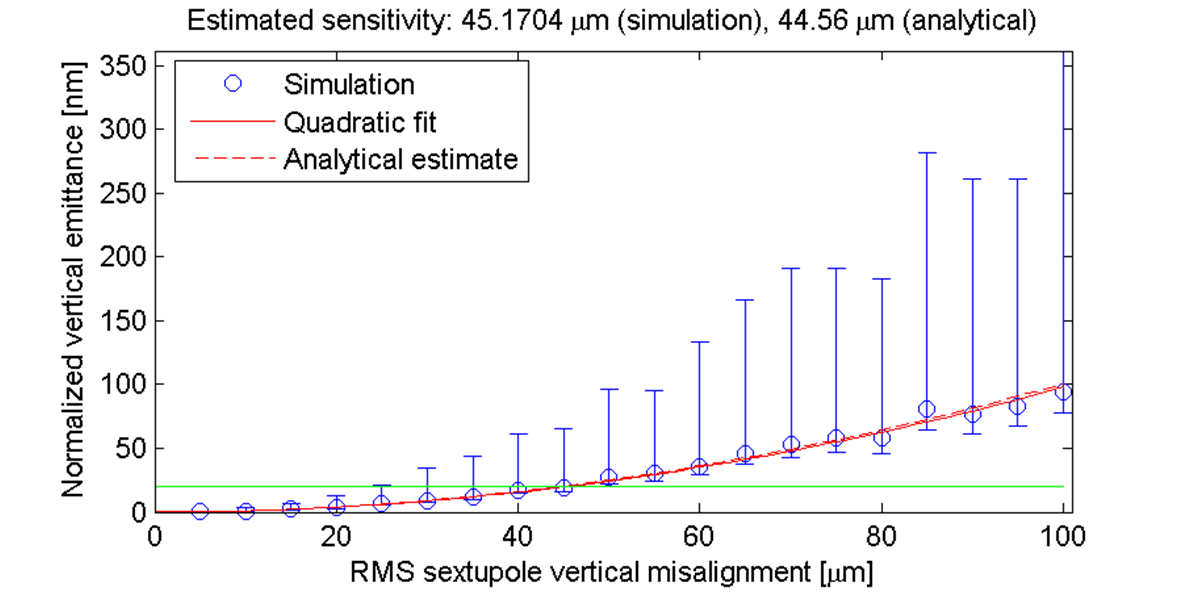
Figure 16: Simulation of vertical emittance resulting from sextupole alignment errors in a storage ring [19]. Each circle shows the mean of the normalised vertical emittance $(\gamma\varepsilon_{y})$ from 100 different sets (seeds) of random alignment errors on the sextupoles; the error bars show the range covered by 90% of the seeds. The solid red line shows a quadratic fit to the circles; the broken red line (very close to the solid red line) shows an analytical estimate of the emittance based on the known sextupole strengths and lattice functions, using equations (230), (237) to estimate the coupling contribution, and (245) and (257) to estimate the dispersion contribution.

4.4 Accurate computation of emittance

The formulae we have derived so far are useful for developing a ‘feel’ for how the vertical emittance depends on magnet alignment errors, and for making rough estimates of the sensitivity to particular types of error. For detailed studies, including modelling and simulations, we need more accurate formulae for computing the vertical emittance in a storage ring with a given set of alignment errors. The calculations involved then become quite complex, and need to be solved using a computer.

There are three methods commonly used for computing the equilibrium emittances in complex lattices with known errors. First, there is a technique based on the usual formulae for the emittances expressed in terms of the radiation integrals, but generalised to the normal modes (see, for example, [20]). Second, there is Chao’s method [21], which involves integrating the eigenvectors of the single-turn transfer matrix around the circumference of the ring. Finally, there is the ‘envelope’ method [22], in which the second order moments of the equilibrium beam distribution are first computed from the single-turn transfer map (including radiation damping and quantum excitation); then the emittances are obtained from the matrix describing the beam distribution. We shall discuss briefly each of these techniques in turn.

First, we consider the method for computing the equilibrium emittances based on normal mode analysis. Let us assume that we have a lattice code that will compute the symplectic single-turn transfer matrix at any point in a given lattice. In general, the transfer matrix will have non-zero terms off the block-diagonals: these terms represent coupling between the horizontal, vertical, and longitudinal motion. The expression (181) we derived for the natural emittance assumed no betatron coupling, and that the coupling between the horizontal and longitudinal motion was relatively weak. However, we can generalise the formula to the case that betatron coupling is present. We still need to assume that the longitudinal motion is weakly coupled to each of the transverse degrees of freedom (i.e. the horizontal and vertical motion). In that case, we can consider separately the $4\times 4$ single-turn transfer matrix $R_{\perp}$ describing the transverse motion:

$$R=\left(\begin{array}[]{cc}R_{\perp}&\bullet\\ \bullet&R_{\parallel}\end{array}\right).$$ (258)

$R_{\parallel}$ is a $2\times 2$ matrix describing the longitudinal motion, and we assume we can neglect the terms represented by the bullets ($\bullet$).

Now we look for a transformation, represented by a $4\times 4$ matrix $V$, that puts $R_{\perp}$ into block-diagonal form, i.e. that ‘decouples’ the transverse motion:

$$\tilde{R}_{\perp}=V\,R_{\perp}\,V^{-1}=\left(\begin{array}[]{cc}R_{\textrm{I}}&0\\ 0&R_{\textrm{II}}\end{array}\right).$$ (259)

$R_{\textrm{I}}$ and $R_{\textrm{II}}$ are $2\times 2$ matrices describing betatron motion in a coordinate system in which the motion appears uncoupled. There are various recipes for constructing the decoupling transformation $V$ (which is not unique): see, for example [23, 24]. Having obtained the matrices describing the uncoupled motion, we can derive the Courant–Snyder parameters for the normal mode motion in the usual way. For example, we can write:

$$R_{\textrm{II}}=\left(\begin{array}[]{cc}\cos\mu_{\textrm{II}}+\alpha_{\textrm{II}}\sin\mu_{\textrm{II}}&\beta_{\textrm{II}}\sin\mu_{\textrm{II}}\\ -\gamma_{\textrm{II}}\sin\mu_{\textrm{II}}&\cos\mu_{\textrm{II}}-\alpha_{\textrm{II}}\sin\mu_{\textrm{II}}\end{array}\right),$$ (260)

and similarly for mode I. We can also obtain the normal mode dispersion functions, by applying the transformation $V$ to a vector constructed from the dispersion functions in the original Cartesian co-ordinates. Then, we can construct the $\mathcal{H}$ function for each mode; for example:

$$\mathcal{H}_{\textrm{II}}=\gamma_{\textrm{II}}\eta_{\textrm{II}}^{2}+2\alpha_{\textrm{II}}\eta_{\textrm{II}}\eta_{p,\textrm{II}}+\beta_{\textrm{II}}\eta_{p,\textrm{II}}^{2}.$$ (261)

Finally, we can write for the mode II emittance:

$$\varepsilon_{\textrm{II}}=C_{q}\gamma^{2}\frac{I_{5,\textrm{II}}}{I_{2}-I_{4,\textrm{II}}},$$ (262)

and similarly for mode I.

For many storage rings, equation (262) works well, and gives an accurate result. However, if there is strong coupling between the transverse and the longitudinal motion (which can happen, for example, for large values of the synchrotron tune), then the approximations needed to derive equation (262) start to break down.

As an alternative to the normal mode analysis, we can consider Chao’s method [21] for computing the emittances, which provides a formula that can be expressed in a convenient form, though it is not always easy to apply. It is again based on the single-turn transfer matrix, but it is more accurate than the ‘decoupling’ method, since it uses the full $6\times 6$ transfer matrix, and does not assume weak coupling between the longitudinal and transverse motion. We do not explain here the physics behind the formula, but simply quote the result:

$$\varepsilon_{k}=C_{L}\frac{\gamma^{5}}{c\alpha_{k}}\oint\frac{|E_{k\,5}(s)|^{2}}{|\rho(s)|^{3}}\,ds,$$ (263)

where $k=$ I, II, III is an index that specifies a particular degree of freedom, the eigenvalues of the single-turn matrix including radiation damping are $e^{-\alpha_{k}\pm 2\pi i\nu_{k}}$, $E_{k\,5}$ is the fifth component of the $k^{\textrm{th}}$ eigenvector of the symplectic single-turn matrix, and:

$$C_{L}=\frac{55}{48\sqrt{3}}\frac{r_{c}\hbar}{m},$$ (264)

where $r_{c}$ is the classical radius and $m$ the mass of the particles in the beam.

Finally, we mention the envelope method [22]. Like Chao’s method, it gives accurate results for the emittances even if there is strong coupling between all three degrees of freedom. The envelope method is based on finding the equilibrium beam distribution described by the Sigma matrix:

$$\Sigma=\left(\begin{array}[]{cccccc}\langle x^{2}\rangle&\langle xp_{x}\rangle&\langle xy\rangle&\langle xp_{y}\rangle&\langle xz\rangle&\langle x\delta\rangle\\ \langle p_{x}x\rangle&\langle p_{x}^{2}\rangle&\langle p_{x}y\rangle&\langle p_{x}p_{y}\rangle&\langle p_{x}z\rangle&\langle p_{x}\delta\rangle\\ \langle yx\rangle&\langle yp_{x}\rangle&\langle y^{2}\rangle&\langle yp_{y}\rangle&\langle yz\rangle&\langle y\delta\rangle\\ \langle p_{y}x\rangle&\langle p_{y}p_{x}\rangle&\langle p_{y}y\rangle&\langle p_{y}^{2}\rangle&\langle p_{y}z\rangle&\langle p_{y}\delta\rangle\\ \langle zx\rangle&\langle zp_{x}\rangle&\langle zy\rangle&\langle zp_{y}\rangle&\langle z^{2}\rangle&\langle z\delta\rangle\\ \langle\delta x\rangle&\langle\delta p_{x}\rangle&\langle\delta y\rangle&\langle\delta p_{y}\rangle&\langle\delta z\rangle&\langle\delta^{2}\rangle\end{array}\right)$$ (265)

This is a symmetric matrix, constructed from the second order moments of all possible combinations of the dynamical variables. For simplicity, we assume in what follows that the first order moments are all zero, i.e. that the closed orbit lies along the reference trajectory. However, the method is easily generalised to include cases where there is closed orbit distortion. In the absence of coupling, the Sigma matrix will be block diagonal. We are interested in the more general case, where coupling is present.

Under a single turn around an accelerator, $\Sigma$ transforms as:

$$\Sigma\mapsto R\Sigma R^{\textrm{T}}+D,$$ (266)

where $R$ is the single-turn transfer matrix (including radiation damping) and $D$ is a constant matrix representing the effects of quantum excitation. From knowledge of the properties of synchrotron radiation, we can compute the matrices $R$ and $D$ for a given lattice design: this will be discussed further below, where we shall give explicit expressions for the transfer matrices in a dipole, including radiation effects.

The equilibrium distribution $\Sigma_{\textrm{eq}}$ has the property:

$$\Sigma_{\textrm{eq}}=R\Sigma_{\textrm{eq}}R^{\textrm{T}}+D.$$ (267)

For given $R$ and $D$, we can solve equation (267) to find $\Sigma_{\textrm{eq}}$, and then from $\Sigma_{\textrm{eq}}$ we can find the invariant emittances, i.e. the conserved quantities under symplectic transport. For any beam distribution $\Sigma$, the invariant emittances $\varepsilon_{k}$ are given by:

$$\textrm{eigenvalues}(\Sigma S)=\pm i\varepsilon_{k},$$ (268)

where $S$ is the antisymmetric block-diagonal matrix (9). To see that this is the case, consider the (simpler) case of motion in one degree of freedom. The Sigma matrix in this case is:

$$\Sigma=\left(\begin{array}[]{cc}\langle x^{2}\rangle&\langle xp_{x}\rangle\\ \langle p_{x}x\rangle&\langle p_{x}^{2}\rangle\end{array}\right)=\left(\begin{array}[]{cc}\beta_{x}&-\alpha_{x}\\ -\alpha_{x}&\gamma_{x}\end{array}\right)\varepsilon_{x}.$$ (269)

In one degree of freedom, the matrix corresponding to (9) is:

$$S=\left(\begin{array}[]{cc}0&1\\ -1&0\end{array}\right).$$ (270)

Then, the eigenvalues of $\Sigma S$ are $\pm i\varepsilon_{x}$. Now, we can show that (under certain assumptions) the emittance is conserved as a bunch is transported along a beam line. In any number of degrees of freedom, the linear transformation in phase space co-ordinates of a particle in the bunch between two points in the beam line can be represented by a matrix $R$:

$$\vec{x}\mapsto R\vec{x},$$ (271)

where $\vec{x}$ is a vector whose components are the phase space variables $x_{i}$.

Now consider how the Sigma matrix transforms. The Sigma matrix can be written as the product of the phase-space co-ordinates averaged over the bunch:

$$\Sigma_{ij}=\langle x_{i}x_{j}\rangle,$$ (272)

where $\Sigma_{ij}$ is the $(i,j)$ component of the Sigma matrix, and the $x_{i}$ are the dynamical variables. The brackets $\langle\cdot\rangle$ indicate an average over all particles in the bunch. Then, using (271), it follows that under a transformation $R$ of the dynamical variables, the Sigma matrix transforms as:

$$\Sigma\mapsto R\Sigma R^{\textrm{T}}.$$ (273)

Since $S$ is a constant matrix, it immediately follows that:

$$\Sigma S\mapsto R\Sigma R^{\textrm{T}}S.$$ (274)

Then, using the fact that $R$ is symplectic (8), we have:

$$\Sigma S\mapsto R\Sigma SR^{-1}.$$ (275)

This is a similarity transformation of $\Sigma S$: the eigenvalues of any matrix are conserved under a similarity transformation. Therefore, since the eigenvalues of $\Sigma S$ give the emittance of the bunch, it follows that the emittances are conserved under linear, symplectic transport.

This argument applies for any number of degrees of freedom. We define the matrix $S$ in three degrees of freedom by (9). The six eigenvalues of $\Sigma S$ are then $\pm i\varepsilon_{k}$, where $k$ is an index ranging over the different degrees of freedom. The quantities $\varepsilon_{k}$ are all conserved under linear, symplectic transport. Even if, as is generally the case, the Sigma matrix is not block-diagonal (i.e. if there is coupling present), then we can still find three invariant emittances using this method, without any modification.

Neglecting radiaton, if $R$ is a (symplectic) matrix that represents the linear single-turn transformation at some point in a storage ring, then an invariant or ‘matched’ distribution is one that satisfies:

$$\Sigma\mapsto R\Sigma R^{\textrm{T}}=\Sigma.$$ (276)

In general, all the particles in the bunch change position in phase space after one turn around the ring: but for a matched distribution, the second order moments remain the same. Although this condition determines the lattice functions (which can be found from the eigenvectors of $\Sigma S$), it is not sufficient to determine the emittances. In other words, the matched distribution condition determines the shape of the bunch, but not the size of the bunch. This makes sense: after all, in a proton storage ring, we can have a matched bunch of any emittance. However, in an electron storage ring, we know that radiation effects will damp the emittances to some equilibrium values. We shall now show how to apply the concept of a matched distribution, when radiation effects are included, to find the equilibrium emittances in an electron storage ring.

To account for radiation effects in an electron storage ring, we must make two modifications to the single-turn transformation. First, the matrix $R$ will no longer be symplectic: this accounts for radiation damping. Second, as well as first order terms in the transformation (represented by the matrix $R$), there will be zeroth order terms: these will correspond to the quantum excitation. The condition for a matched distribution should then be written:

$$\Sigma=R\Sigma R^{\textrm{T}}+D,$$ (277)

where $R$ and $D$ are constant, non-symplectic matrices that represent the first order and zeroth order terms in the single-turn transformation, respectively. Equation (277) is sufficient to determine the Sigma matrix uniquely – in other words, using just this equation (with known $R$ and $D$) we can find the bunch emittances and the matched lattice functions.

The envelope method for finding the equilibrium emittances in a storage ring then consists of three steps. First, we need to find the first order terms $R$ and zeroth order terms $D$ in the single-turn transformation:

$$\Sigma\mapsto R\Sigma R^{\textrm{T}}+D.$$ (278)

In the second step, we use the matching condition (277) to determine the Sigma matrix. Then, in the third and final step, we find the equilibrium emittances from the eigenvalues of $\Sigma S$.

Strictly speaking, since $R$ is not symplectic, the emittances are not invariant as the bunch moves around the ring. Therefore, we may expect to find a different emittance at each point around the ring. However, if radiation effects are fairly small, then the variations in the emittances will also be small.

The transfer matrices $R$ and $D$ for an entire ring can be constructed from the transfer matrices for individual components in the ring. As an example, we shall consider a thin ‘slice’ of a dipole. This is an important case, since in most storage rings, radiation effects are significant only in dipoles. Furthermore, complete dipoles can be constructed by composing the maps for a number of slices. Hence, once we have a map for a thin slice of dipole, and knowing the usual (symplectic) transfer maps for drift spaces, quadrupoles and rf cavities, we will be able to construct the map for one complete turn of a storage ring, starting at any point.

Recall that the transformations for the phase space variables in the emission of radiation carrying momentum $dP$ are:

$$x \mapsto x,$$ (279)

$$p_{x} \mapsto \left(1-\frac{dP}{P_{0}}\right)p_{x},$$ (280)

$$y \mapsto y,$$ (281)

$$p_{y} \mapsto \left(1-\frac{dP}{P_{0}}\right)p_{y},$$ (282)

$$z \mapsto z,$$ (283)

$$\delta \mapsto \delta-\frac{dP}{P_{0}},$$ (284)

where $P_{0}$ is the reference momentum. In general, $dP$ is a function of the co-ordinates. To find the transformation matrices $R$ and $D$, we find an explicit expression for $dP/P_{0}$, and then write down the above transformations to first order. For an ultra-relativistic particle, the momentum lost through radiation can be expressed in terms of the synchrotron radiation power $P_{\gamma}$ (energy loss per unit time):

$$\frac{dP}{P_{0}}\approx\frac{P_{\gamma}}{E_{0}}dt\approx\frac{P_{\gamma}}{E_{0}}\left(1+\frac{x}{\rho}\right)\frac{ds}{c},$$ (285)

where $\rho$ is the radius of curvature of the reference trajectory. The radiation power $P_{\gamma}$ is given by (31). In general, the dipole may have a quadrupole gradient, so the field is:

$$B=B_{0}+B_{1}x.$$ (286)

Also, the particle may have some energy deviation, so the total energy is:

$$E=E_{0}(1+\delta).$$ (287)

Substituting these expressions, we find (after some manipulation):

$$P_{\gamma}=c\frac{C_{\gamma}}{2\pi}\left(\frac{1}{\rho^{2}}+2k_{1}\frac{x}{\rho}\right)(1+\delta)^{2}E_{0}^{4},$$ (288)

where $k_{1}$ is the normalised quadrupole gradient in the dipole:

$$k_{1}=\frac{q}{P_{0}}B_{1}.$$ (289)

Hence, the normalised momentum loss may be written:

$$\frac{dP}{P_{0}}\approx\frac{C_{\gamma}}{2\pi}\left(\frac{1}{\rho^{2}}+2k_{1}\frac{x}{\rho}\right)\left(1+\frac{x}{\rho}\right)(1+\delta)^{2}E_{0}^{3}\,ds.$$ (290)

Expanding to first order in the phase space variables, we can write:

$$\frac{dP}{P_{0}}\approx\frac{C_{\gamma}}{2\pi}\frac{E_{0}^{3}}{\rho^{2}}\,ds+\frac{C_{\gamma}}{2\pi}\left(\frac{1}{\rho^{2}}+2k_{1}\frac{x}{\rho}\right)\frac{E_{0}^{3}}{\rho}x\,ds+2\frac{C_{\gamma}}{2\pi}\frac{E_{0}^{3}}{\rho^{2}}\delta\,ds+O(x^{2})+O(\delta^{2}).$$ (291)

Given the expression (291) for $dP/P_{0}$, the transformations (279)–(284) become (to first order in the dynamical variables):

$$x \mapsto x,$$ (292)

$$p_{x} \mapsto \left(1-\frac{C_{\gamma}}{2\pi}\frac{E_{0}^{3}}{\rho^{2}}\,ds\right)p_{x},$$ (293)

$$y \mapsto y,$$ (294)

$$p_{y} \mapsto \left(1-\frac{C_{\gamma}}{2\pi}\frac{E_{0}^{3}}{\rho^{2}}\,ds\right)p_{y},$$ (295)

$$z \mapsto z,$$ (296)

$$\delta \mapsto \left(1-2\frac{C_{\gamma}}{2\pi}\frac{E_{0}^{3}}{\rho^{2}}\,ds\right)\delta-\frac{C_{\gamma}}{2\pi}\left(\frac{1}{\rho^{2}}+2k_{1}\frac{x}{\rho}\right)\frac{E_{0}^{3}}{\rho}x\,ds-\frac{C_{\gamma}}{2\pi}\frac{E_{0}^{3}}{\rho^{2}}\,ds.$$ (297)

The first order terms give the components of $R_{\textrm{dip}}(ds)$, the transfer matrix for a thin slice (length $ds$) of a dipole. There is a zeroth order term in the map for the dynamical variables that will contribute to (the (6,6) component of) $D_{\textrm{dip}}(ds)$, which contains the zeroth order terms in the transformation of the Sigma matrix through a thin slice of a dipole. Since the (6,6) component of $D_{\textrm{dip}}(ds)$ represents the quantity $\langle\Delta\delta^{2}\rangle$, the contribution to this component from the zeroth order term in (297) will be second order in $ds$. We still have to take proper account of the quantum nature of the radiation. This will make an additional contribution to $D_{\textrm{dip}}(ds)$.

The zeroth order term in the map for the Sigma matrix is given by:

$$\left[D_{\textrm{dip}}(ds)\right]_{66}=\left\langle\left(\frac{dP}{P_{0}}\right)^{\!\!2}\right\rangle\approx\frac{\langle u^{2}\rangle}{E_{0}^{2}},$$ (298)

where $\langle u^{2}\rangle$ is the mean square of the photon energy. Using (102), we find that, to zeroth order in the phase space variables:

$$\left\langle\left(\frac{dP}{P_{0}}\right)^{\!\!2}\right\rangle\approx 2C_{q}\gamma^{2}\frac{C_{\gamma}}{2\pi}\frac{E_{0}^{3}}{\rho^{3}}\,ds.$$ (299)

Note that this term is first order in $ds$, whereas the contribution to $D_{\textrm{dip}}(ds)$ that we found previously was second order in $ds$. Hence, in the limit $ds\to 0$, the latter contribution dominates over the previous contribution.

Collecting the above results, and taking only dominant contributions in the limit $ds\to 0$, we find that the radiation in a thin slice of dipole has an effect on the Sigma matrix that can be represented by:

$$\Sigma\mapsto R_{\textrm{dip}}(ds)\Sigma R_{\textrm{dip}}^{\textrm{T}}(ds)+D_{\textrm{dip}}(ds),$$ (300)

where:

$$R_{\textrm{dip}}(ds)=\left(\begin{array}[]{cccccc}1&0&0&0&0&0\\ 0&1-\frac{C_{\gamma}}{2\pi}\frac{E_{0}^{3}}{\rho^{2}}ds&0&0&0&0\\ 0&0&1&0&0&0\\ 0&0&0&1-\frac{C_{\gamma}}{2\pi}\frac{E_{0}^{3}}{\rho^{2}}ds&0&0\\ 0&0&0&0&1&0\\ -\frac{C_{\gamma}}{2\pi}\left(\frac{1}{\rho^{2}}+2k_{1}\right)\frac{E_{0}^{3}}{\rho}ds&0&0&0&0&1-2\frac{C_{\gamma}}{2\pi}\frac{E_{0}^{3}}{\rho^{2}}ds\end{array}\right),$$ (301)

and:

$$D_{\textrm{dip}}(ds)=\left(\begin{array}[]{cccccc}0&0&0&0&0&0\\ 0&0&0&0&0&0\\ 0&0&0&0&0&0\\ 0&0&0&0&0&0\\ 0&0&0&0&0&0\\ 0&0&0&0&0&2C_{q}\gamma^{2}\frac{C_{\gamma}}{2\pi}\frac{E_{0}^{3}}{\rho^{3}}ds.\end{array}\right).$$ (302)

To construct the full single-turn transformation, we need to compose the maps for all the elements in the ring, including the radiation effects in the dipoles. It is straightforward to do this numerically using a computer. However, some care is needed in handling the $D$ matrices. For example, given the Sigma matrix at a location $s_{0}$, we find the Sigma matrix at a location $s_{1}=s_{0}+ds$ from:

$$\Sigma(s_{1})=R(s_{1};s_{0})\Sigma(s_{0})R^{\textrm{T}}(s_{1};s_{0})+D(s_{1};s_{0}).$$ (303)

Then the Sigma matrix at $s_{2}$ is given by:

$$\Sigma(s_{2}) = R(s_{2};s_{1})\Sigma(s_{1})R^{\textrm{T}}(s_{2};s_{1})+D(s_{2};s_{1})$$ (304)

$$= R(s_{2};s_{0})\Sigma(s_{0})R^{\textrm{T}}(s_{2};s_{0})+R(s_{2};s_{1})D(s_{1};s_{0})R^{\textrm{T}}(s_{2};s_{1})+D(s_{2};s_{1}).$$

Hence:

$$R(s_{2};s_{0}) = R(s_{2};s_{1})R(s_{1};s_{0})$$ (305)

$$D(s_{2};s_{0}) = R(s_{2};s_{1})D(s_{1};s_{0})R^{\textrm{T}}(s_{2};s_{1})+D(s_{2};s_{1}).$$ (306)

Continuing the process, we find:

$$R(s_{n};s_{0}) = R(s_{n};s_{n-1})R(s_{n-1};s_{n-2})\cdots R(s_{1};s_{0})$$ (307)

$$D(s_{n};s_{0}) = \sum_{r=1}^{n}R(s_{n};s_{r})D(s_{r};s_{r-1})R^{\textrm{T}}(s_{n};s_{r})$$ (308)

When composing the transfer maps for thin slices of a dipole, we have to remember to ‘interleave’ the radiation maps with the usual symplectic transport map for a thin slice of dipole.

The next step in finding the equilibrium emittances is to solve the matching condition (277) to find the Sigma matrix for the equilibrium distribution. To do this (for given matrices $R$ and $D$), we make use of the eigenvectors $U$ of $R$, and the diagonal matrix $\Lambda$ constructed from the eigenvalues of $R$:

$$RU=\Lambda U.$$ (309)

Defining $\tilde{\Sigma}$ and $\tilde{D}$ by:

$$\Sigma = U\tilde{\Sigma}U^{\textrm{T}},$$ (310)

$$D = U\tilde{D}U^{\textrm{T}},$$ (311)

the solution for the Sigma matrix can be written:

$$\tilde{\Sigma}_{ij}=\frac{\tilde{D}_{ij}}{1-\Lambda_{i}\Lambda_{j}}.$$ (312)

The above formulae enable us to find the matched (equilibrium) distribution $\Sigma$; the eigenvalues of $\Sigma S$ are then $\pm i\varepsilon_{k}$, where $\varepsilon_{k}$ are the emittances.

The envelope method makes explicit the fact that vertical emittance is generated by coupling between the vertical and longitudinal planes in regions where radiation is emitted (i.e. by vertical dispersion in dipoles), and by coupling between the vertical and horizontal planes in regions where radiation is emitted (i.e. by betatron coupling in dipoles). Here, we need to be careful in the use of the term ‘coupling’. In this context, coupling means the presence of non-zero components off the block-diagonals in the single-turn matrix, $R$. Full characterisation of the coupling requires complete specification of all the components off the block-diagonals in $R$. Depending on these components, it is possible to have coupling in a storage ring, and not generate any vertical emittance. For example, one could construct a closed ‘coupling bump’ using sets of skew quadrupoles in a straight section in a storage ring. With proper care in the design, outside the region between the skew quadrupoles, the vertical motion can be completely decoupled from the horizontal and the longitudinal. Then, despite the presence of strong coupling in some parts of the storage ring, the equilibrium vertical emittance will come only from the opening angle of the cone describing the spatial distribution of the synchrotron radiation.

Numerical computational procedures (such as the envelope method) for finding the equilibrium beam distribution in a storage ring are important because they provide ways to calculate the equilibrium emittances in complex, coupled lattices. It is possible to include other non-symplectic effects in the calculation (such as, for example, intrabeam scattering).

4.5 Ultra-low emittance tuning

Often, coupling comes from magnet alignment errors, which will not be known completely in an operating machine. At the design stage, it is important to characterise the sensitivity of a lattice to magnet alignment errors, particularly regarding the vertical emittance. Being able to compute the beam emittances in a storage ring with coupling errors present makes it possible to simulate the effects of various types and sizes of alignment error – and then to optimise the lattice design to minimise the sensitivity to the likely errors. However, in practice, tuning a storage ring to achieve a vertical emittance of no more than a few picometres (which may be required for some applications) is a considerable challenge, even in a lattice designed so as to minimise the sensitivity to coupling errors. Accurate alignment (by survey) of the magnets is always the first step in achieving ultra-low emittances; but beam-based tuning methods will then also be needed.

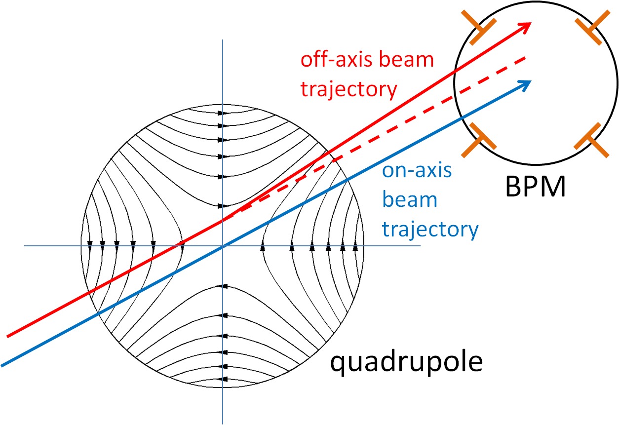
Figure 17: Beam-based alignment in a quadrupole. If the beam passes off-axis through a quadrupole magnet, then varying the strength of the magnet changes the trajectory downstream of the magnet. A change in trajectory can be observed in a beam position monitor (BPM). One method of beam-based alignment consists of steering the beam (using upstream orbit corrector magnets) until changing the quadrupole strength has no effect on the beam position observed in the BPM.

A variety of beam-based methods for tuning storage rings have been developed over the years. A typical procedure might look as follows:

1. Align the magnets by a survey of the ring. Typically, quadrupoles need to be aligned to better than a few tens of microns, and sextupoles to better than a couple of hundred microns.

2. Determine the positions of the BPMs relative to the quadrupoles. This is known as ‘beam-based alignment’ (BBA, see Fig. 17), and can be achieved by steering the beam to a position in each quadrupole where changing the quadrupole strength has no effect on the orbit [25].

3. Correct the orbit (using steering magnets) so that it is as close as possible to the centres of the quadrupoles.

4. Correct the vertical dispersion (using steering magnets and/or skew quadrupoles, and measuring the dispersion at the BPMs) as close to zero as possible.

5. Correct the coupling, by adjusting skew quadrupoles so that an orbit ‘kick’ in one plane (from any orbit corrector) has no effect on the orbit in the other plane.

Usually, the last three steps need to be iterated several (or even many) times.

Results from the tuning procedure described above can be limited by systematic errors on the BPMs, which can affect dispersion and coupling measurements. A useful technique for overcoming such limitations is to apply Orbit Response Matrix (ORM) analysis [26]. This can be used to determine a wide range of magnet and diagnostics parameters, including coupling errors and BPM tilts. Although vertical emittances of order 1 pm have now been achieved (representing an emittance ratio of less than 0.1%), tuning an electron storage ring to operate in this regime still remains a challenging goal, requiring extensive work and application of a range of techniques to reduce errors. Even making measurements of emittances less than a few picometres is not straightfoward, and requires specialist instrumentation (see, for example, [27]).

References

- [1] J.A. Clarke, The science and technology of undulators and wigglers, Oxford University Press, Oxford, UK (2004).
- [2] H. Goldstein, C.P. Poole Jr. and J.L. Safko, Classical mechanics, 3rd edition, Addison–Wesley, Boston, MA, USA (2001).
- [3] E.D. Courant and H.S. Snyder, Theory of the alternating gradient synchrotron, Annals of Physics 3, pp. 1–48 (1958).
- [4] A. Wolski, Alternative approach to general coupled linear optics, Phys. Rev. ST Accel. Beams 9, 024001 (2006).
- [5] J.D. Jackson, Classical electrodynamics, 3rd edition, John Wiley and Sons, New York, NY, USA (1998).
- [6] M. Sands, The physics of electron storage rings – an introduction, Technical Report SLAC–121, Stanford Linear Accelerator Centre, Stanford, CA, USA (1970).
- [7] H. Wiedemann, Particle accelerator physics, 3rd edition, Springer, Berlin, Germany (2007).
- [8] K.W. Robinson, Radiation effects in circular electron accelerators, Physical Review 111, 2, pp. 373–380 (1958).
- [9] T.O. Raubenheimer, The generation and acceleration of low emittance flat beams for future linear colliders, Technical Report SLAC–R–387, Stanford Linear Accelerator Centre, Stanford, CA, USA (1991).
- [10] R. Chasman, G.K. Green and E.M. Rowe, Preliminary design of a dedicated synchrotron radiation facility, IEEE Transactions on Nuclear Science NS–22, 3, pp. 1765–1767 (1975)
- [11] S.Y. Lee and L. Teng, Theoretical minimum emittance lattice for an electron storage ring, Proceedings of the 1991 Particle Accelerator Conference, San Francisco, CA, USA (1991).
- [12] A. Ropert, L. Farvacque, J. Jacob, J.L. Laclare, E. Plouviez, J.L. Revol, K. Scheidt, Accelerator physics trends at the ESRF, Proceedings of the 1995 Particle Accelerator Conference, Dallas, TX, USA (1995).
- [13] A. Jackson, Commissioning and performance of the Advanced Light Source, Proceedings of the 1993 Particle Accelerator Conference, Washington, DC, USA (1993).
- [14] A. Streun et al., Commissioning of the Swiss Light Source, Proceedings of the 2001 Particle Accelerator Conference, Chicago, IL, USA (2001).
- [15] S.C. Leemann, Å. Andersson, M. Eriksson, L.-J. Lindgren and E. Wallén, Beam dynamics and expected performance of Sweden’s new storage-ring light source: MAX IV, Phys. Rev. ST Accel. Beams 12, 120701 (2009).
- [16] J. Guo and T. Raubenheimer, Low emittance e-/e+ storage ring design using bending magnets with longitudinal gradient, Proceedings of the European Particle Accelerator Conference 2002, Paris, France (2002).
- [17] R. Dowd, M. Boland, G. LeBlanc and Y.-R.E. Tan, Achievement of ultralow emittance coupling in the Australian Synchrotron storage ring, Phys. Rev. ST Accel. Beams 14, 012804 (2011).
- [18] M. Aiba, M. Böge, N. Milas, A. Streun, Ultra low vertical emittance at SLS through systematic and random optimization, Nucl. Instr. Meth. Phys. Res. A, 694, pp. 133–139 (2012).
- [19] A. Wolski, J. Gao, S. Guiducci (editors), Configuration studies and recommendations for the ILC Damping Rings, Technical Report LBNL–59449 (2006).
- [20] D. Sagan, The Bmad reference manual, \urlhttp://www.lepp.cornell.edu/ dcs/bmad/ (2013).
- [21] A. Chao, Evaluation of beam distribution parameters in an electron storage ring, J. Appl. Phys. 50, pp. 595–598 (1979).
- [22] K. Ohmi, K. Hirata, K. Oide, From the beam-envelope matrix to the synchrotron radiation integrals, Phys. Rev. E 49, pp.751–765 (1994).
- [23] D.A. Edwards and L.C. Teng, Parameterization of linear coupled motion in periodic systems, IEEE Transactions on Nuclear Science NS–20, 3, pp. 885–888 (1973)
- [24] D. Sagan and D. Rubin, Linear analysis of coupled lattices, Phys. Rev. ST Accel. Beams 2, 074001 (1999).
- [25] F. Zimmermann and M.G. Minty, Measurement and control of charged particle beams, Springer, Berlin, Germany (2003).
- [26] J. Safranek, Experimental determination of storage ring optics using orbit response measurements, Nucl. Instr. Meth. Phys. Res. A, 388, 1, pp. 27–36 (1997).
- [27] Å. Andersson, M. Böge, A. Lüdeke, V. Schlott, A. Streun, Determination of a small vertical electron beam profile and emittance at the Swiss Light Source, Nucl. Instr. Meth. Phys. Res. A, 591, 3, pp. 437–446 (2008).