.

TIME-RESOLVED PHOTOELECTRON SPECTROSCOPY OF NON-ADIABATIC DYNAMICS IN POLYATOMIC MOLECULES
Published in Advances in Chemical Physics, Volume 139 (ed S. A. Rice), John Wiley & Sons, Inc., Hoboken, NJ, USA. doi: 10.1002/9780470259498.ch6

*

Chapter Introduction

The photodynamics of polyatomic molecules generally involves complex intramolecular processes which rapidly redistribute both charge and vibrational energy within the molecule. The coupling of vibrational and electronic degrees of freedom leads to the processes known as radiationless transitions, internal conversion, isomerization, proton and electron transfer etc. [Bixon1968, Jortner1969, Henry1973, Freed1976, Stock1997, Worth2004, Klessinger1994, Koppel1984]. These non-adiabatic dynamics underlie the photochemistry of almost all polyatomic molecules [Michl1990] and are important in photobiological processes such as vision and photosynthesis [Schoenlein1991], and underlie many concepts in active molecular electronics [Jortner1997]. The coupling of charge with energy flow is often understood in terms of the breakdown of the Born-Oppenheimer approximation (BOA), an adiabatic separation of electronic from nuclear motions. The BOA allows the definition of the nuclear potential energy surfaces that describe both molecular structures and nuclear trajectories, thereby permitting a mechanistic picture of molecular dynamics. The breakdown of the BOA is uniquely due to nuclear dynamics and occurs at the intersections or near intersections of potential energy surfaces belonging to different electronic states. Non-adiabatic coupling often leads to complex, broadened absorption spectra due to the high density of nuclear states and strong variations of transition dipole with nuclear coordinate. In this situation, the very notion of distinct and observable vibrational and electronic states is obscured. The general treatment of these problems remains one of the most challenging problems in molecular physics, particularly when the state density becomes high and multi-mode vibronic couplings are involved. Our interest is in developing time-resolved methods for the experimental study of non-adiabatic molecular dynamics. The development of femtosecond methods for the study of gas-phase chemical dynamics is founded upon the seminal studies of A.H. Zewail and co-workers, as recognized in 1999 by the Nobel Prize in Chemistry [Zewail2000]. This methodology has been applied to chemical reactions ranging in complexity from bond-breaking in diatomic molecules to dynamics in larger organic and biological molecules.

Femtosecond time-resolved methods involve a pump-probe configuration in which an ultrafast pump pulse initiates a reaction or, more generally, creates a nonstationary state or wavepacket, the evolution of which is monitored as a function of time by means of a suitable probe pulse. Time-resolved or wavepacket methods offer a view complementary to the usual spectroscopic approach and often yield a physically intuitive picture. Wave packets can behave as zeroth-order or even classical-like states and are therefore very helpful in discerning underlying dynamics. The information obtained from these experiments is very much dependent on the nature of the final state chosen in a given probe scheme. Transient absorption and nonlinear wave mixing are often the methods of choice in condensed-phase experiments because of their generality. In studies of molecules and clusters in the gas phase, the most popular methods, laser-induced fluorescence and resonant multiphoton ionization, usually require the probe laser to be resonant with an electronic transition in the species being monitored. However, as a chemical reaction initiated by the pump pulse evolves toward products, one expects that both the electronic and vibrational structures of the species under observation will change significantly and some of these probe methods may be restricted to observation of the dynamics within a small region of the reaction coordinate.

We focus here upon gas-phase time-resolved photoelectron spectroscopy (TRPES) of neutral polyatomic molecules. TRPES is particularly well suited to the study of ultrafast non-adiabatic processes because photoelectron spectroscopy is sensitive to both electronic configurations and vibrational dynamics [Eland1984]. Due to the universal nature of ionization detection, TRPES has been demonstrated to be able to follow dynamics along the entire reaction coordinate. In TRPES experiments, a time-delayed probe laser generates free electrons via photoionization of the evolving excited state, and the electron kinetic energy and/or angular distribution is measured as a function of time. As a probe, TRPES has several practical and conceptual advantages [Fischer1995]: (a) Ionization is always an allowed process, with relaxed selection rules due to the range of symmetries of the outgoing electron. Any molecular state can be ionized. There are no ’dark’ states in photoionization; (b) Highly detailed, multiplexed information can be obtained by differentially analyzing the outgoing photoelectron as to its kinetic energy and angular distribution; (c) Charged particle detection is extremely sensitive; (d) Detection of the ion provides mass information on the carrier of the spectrum; (e) Higher order (multiphoton) processes, which can be difficult to discern in femtosecond experiments, are readily revealed; (f) Photoelectron-photoion coincidence measurements can allow for studies of cluster solvation effects as a function of cluster size and for time-resolved studies of scalar and vector correlations in photodissociation dynamics. Beginning in 1996, TRPES has been the subject of a number of reviews [Stolow1996, Stolow1998, Hayden2000, Radloff2000, Takatsuka2000, Neumark2001, Suzuki2001, Seideman2002, Reid2003, Stolow2003, Stolow2003a, Suzuki2004, Wollenhaupt2005, Suzuki2006, Hertel2006] and these cover various aspects of the field. An exhaustive review of the TRPES literature, including dynamics in both neutrals and anions, was published recently [Stolow2004]. Therefore, rather than a survey, our emphasis here will be on the conceptual foundations of TRPES and the advantages of this approach in solving problems of non-adiabatic molecular dynamics, amplified by examples of applications of TRPES chosen mainly from our own work.

In the following sections we begin with a review of wavepacket dynamics. We emphasize the aspects of creating and detecting wavepackets and the special role of the final state which acts as a “template” onto which the dynamics is projected. We then discuss aspects of the dynamical problem of interest here, namely the non-adiabatic excited state dynamics of isolated polyatomic molecules. We believe that the molecular ionization continuum is a particularly interesting final state for studying time-resolved non-adiabatic dynamics. Therefore, in some detail, we consider the general process of photoionization and discuss features of single photon photoionization dynamics of excited molecular state and its energy and angle-resolved detection. We briefly review the experimental techniques that are required for laboratory studies of TRPES. As TRPES is more involved than ion detection, we felt it important to motivate the use of photoelectron spectroscopy as a probe by comparing mass-resolved ion yield measurements with TRPES, using the example of internal conversion dynamics in a linear hydrocarbon molecule. Finally, we consider various applications of TRPES, with examples selected to illustrate the general issues that have been addressed.

Chapter Wavepacket dynamics

A Frequency and Time domain perspectives

Time-resolved experiments on isolated systems involve the creation and detection of wavepackets which we define to be coherent superpositions of exact molecular eigenstates $|N\rangle$. By definition, the exact (non Born-Oppenheimer) eigenstates are the solutions to the time-independent Schrödinger equation and are stationary. Time dependence, therefore, can only come from superposition and originates in the differing quantum mechanical energy phase factors $\mathrm{e}^{-iE_{N}t/\hbar}$ associated with each eigenstate. Conceptually, there are three steps to a pump-probe wavepacket experiment: (i) the preparation or pump step; (ii) the dynamical evolution; and (iii) the probing of the non-stationary superposition state.

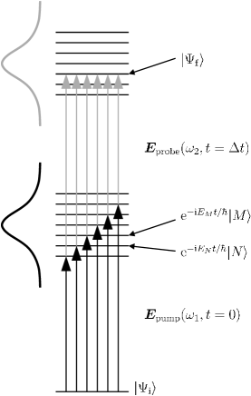
Figure 1: The creation, evolution and detection of wavepackets. The pump laser pulse $\bm{E}_{\mathrm{pump}}$ (black) creates a coherent superposition of molecular eigenstates at $t=0$ from the ground state $|\Psi_{\mathrm{i}}\rangle$. The set of excited state eigenstates $|N\rangle$ in the superposition (wavepacket) have different energy phase factors, leading to non-stationary behaviour (wavepacket evolution). At time $t=\Delta t$ the wavepacket is projected by a probe pulse $\bm{{E}_{\mathrm{probe}}}$ (grey) onto a set of final states $|\Psi_{\mathrm{f}}\rangle$ which act as a “template” for the dynamics. The time-dependent probability of being in a given final state $|\Psi_{\mathrm{f}}\rangle$ is modulated by the interferences between all degenerate coherent two-photon transition amplitudes leading to that final state.

From a frequency domain point of view, a femtosecond pump-probe experiment, shown schematically in Fig. 1, is a sum of coherent two-photon transition amplitudes constrained by the pump and probe laser bandwidths. The measured signal is proportional to the population in the final state $|\Psi_{\mathrm{f}}\rangle$ at the end of the two pulse sequence. As these two-photon transitions are coherent, we must therefore add the transition amplitudes and then square in order to obtain the probability. As discussed below, the signal contains interferences between all degenerate two-photon transitions. When the time delay between the two laser fields is varied, the phase relationships between the two-photon transition amplitudes changes, modifying the interference in the final state. The amplitudes and initial phases of the set of the initially prepared excited eigenstates are determined by the amplitudes and phases of the pump laser field frequencies, and the transition dipole amplitudes between the initial state and the excited state of interest. Once the pump laser pulse is over, the wavepacket $\Psi(t)$ evolves freely according to relative energy phase factors in the superposition as given by

$$|\Psi(t)\rangle=\sum_{N}A_{N}\mathrm{e}^{-iE_{N}t/\hbar}|N\rangle.$$ (1)

The complex coefficients $A_{N}$ contain both the amplitudes and initial phases of the exact molecular eigenstates $|N\rangle$ which are prepared by the pump laser, and the $E_{N}$ are the excited state eigenenergies. The probe laser field interacts with the wavepacket after the pump pulse is over, projecting it onto a specific final state $|\Psi_{f}\rangle$ at some time delay $\Delta t$. This final state is the “template” onto which the wavepacket dynamics are projected. The time dependence of the differential signal, S${}_{f}(\Delta t)$, for projection onto a single final state can be written as

$$S_{f}(t)=\left|\langle\Psi_{f}|\bm{E}_{\mathrm{probe}}(\omega)\cdot\bm{d}|\Psi(t)\rangle\right|^{2}=\left|\sum_{N}B_{N}\mathrm{e}^{-iE_{N}t/\hbar}\right|^{2},$$ (2)

where the complex coefficients $B_{N}$ contain both the wavepacket amplitudes $A_{N}$ and the (complex) probe transition dipole matrix elements connecting each eigenstate in the superposition $|N\rangle$ to the final state,

$$B_{N}=A_{N}\langle\Psi_{f}|\bm{E}_{\mathrm{probe}}(\omega)\cdot\bm{d}|N\rangle.$$ (3)

Eq. (2) may be re-written as

$$S_{f}(t)=2\sum_{N}\sum_{M\leq N}|B_{N}||B_{M}|\cos[(E_{N}-E_{M})t/\hbar+\Phi_{NM}],$$ (4)

where the phase factor $\Phi_{NM}$ contains the initial phase differences of the molecular eigenstates, and the phase difference of the probe transition dipole matrix elements connecting the states $|N\rangle$ and $|M\rangle$ to the final state. The most detailed information is in this final state resolved differential signal S${}_{f}(t)$. It arises from the coherent sum over all two-photon transition amplitudes consistent with the pump and probe laser bandwidths and contains interferences between all degenerate two-photon transitions. It can be seen that the signal as a function of $\Delta t$ contains modulations at frequencies $(E_{N}-E_{M})/\hbar$, corresponding to the set of all level spacings in the superposition. This is the relationship between the wavepacket dynamics and observed pump-probe signal. It is the interference between individual two-photon transitions arising from the initial state, through different excited eigenstates and terminating in the same single final state, which leads to these modulations. The Fourier transform power spectrum of this time domain signal therefore contains frequencies which give information about the set of level spacings in the excited state. The transform, however, also yields the Fourier amplitudes at these frequencies, each corresponding to a modulation depth seen in the time domain data at that frequency. These Fourier amplitudes relate to the overlaps of each excited state eigenfunction within the wavepacket with a specific, chosen final state. Different final states will generally have differing transition dipole moment matrix elements with the eigenstates $|N\rangle$ comprising the wavepacket, and so in general each final state will produce a signal S_f which has different Fourier amplitudes in its power spectrum. For example, if two interfering transitions have very similar overlaps with the final state, they will interfere constructively or destructively with nearly 100% modulation and, hence, have a very large Fourier amplitude at that frequency. Conversely, if one transition has much smaller overlap with the final state (due to e.g. a “forbidden” transition or negligible Franck-Condon overlap) than the other, then the interference term will be small and the modulation amplitude at that frequency will be negligible. Clearly, the form of the pump probe signal will depend on how the final state “views” the various eigenstates comprising the wavepacket. An important point is that by carefully choosing different final states, it is possible for the experimentalist to emphasize and probe particular aspects of the wavepacket dynamics. In general there will be a set of final states which fall within the probe laser bandwidth. We must differentiate, therefore, between integral and differential detection techniques. With integral detection techniques (e.g. total fluorescence, ion yield etc.), the experimentally measured total signal, $S(\Delta t)$, is proportional to the total population in the set of all energetically allowed final states, $\sum_{f}S_{f}(\Delta t)$, created at the end of the two-pulse sequence. Information is clearly lost in carrying out this sum since the individual final states may each have different overlaps with the wavepacket. Therefore, differential techniques such as dispersed fluorescence, translational energy spectroscopy or photoelectron spectroscopy, which can disperse the observed signal with respect to final state, will be important. The choice of the final state is of great importance as it determines the experimental technique and significantly determines the information content of an experiment.

We now consider a pump-probe experiment from a time-domain perspective. The coherent superposition of exact molecular eigenstates constructs, for a short time, a zeroth order state. Zeroth order states are often physically intuitive solutions to a simpler Hamiltonian $H_{0}$, and can give a picture of the basic dynamics of the problem. The full Hamiltonian is then given by $H=H_{0}+V$. Suppose we choose to expand the molecular eigenstates in a complete zeroth-order basis of $H_{0}$ which we denote by $|n\rangle$

$$|N\rangle=\sum_{n}a^{N}_{n}|n\rangle,$$ (5)

then the wavepacket described in Eq. (1) may be written in terms of these basis states as

$$|\Psi(t)\rangle=\sum_{n}C_{n}\mathrm{e}^{-\mathrm{i}(E_{n}+E_{n}^{\mathrm{int}})t/\hbar}|n\rangle,$$ (6)

where the coefficients in the expansion are given by $C_{n}=\sum_{N}a^{N}_{n}A_{N}$ (with $A_{N}$ the eigenstate coefficients in the wavepacket in Eq. (1)). To zeroth-order, the eigenstate $|N\rangle$ is approximated by $|n\rangle$. The time dependence of the wavepacket expressed in the zeroth-order basis reflects the couplings between the basis states $|n\rangle$ which are caused by terms in the full molecular Hamiltonian which are not included in the model Hamiltonian, $H_{0}$. In writing Eq. (6), the eigenenergies of the true molecular eigenstates have been expressed in terms of the eigenenergies of the zeroth-order basis as $E_{N}=E_{n}+E_{n}^{\mathrm{int}}$, where $E_{n}^{\mathrm{int}}$ is the interaction energy of zeroth order state $|n\rangle$ with all other zeroth order states. The wavepacket evolution, when considered in terms of the zeroth-order basis contains frequency components corresponding to the couplings between states, as well as frequency components corresponding to the energies of the zeroth-order states. To second order in perturbation theory, the interaction energy (coupling strength) $E^{\mathrm{int}}_{n}$ between zeroth-order states is given in terms of the matrix elements of $V$ by

$$E_{n}^{\mathrm{int}}=\langle n|V|n\rangle+\sum_{m\not=n}\frac{\langle m|V|n\rangle^{2}}{E_{m}-E_{n}}.$$ (7)

Just as the expansion in the zeroth-order states can describe the exact molecular eigenstates, likewise an expansion in the exact states can be used to prepare, for a short time, a zeroth-order state. If the perturbation $V$ is small, and the model Hamiltonian $H_{0}$ is a good approximation to $H$, then the initially prepared superposition of eigenstates will resemble a zeroth-order state. The dephasing of the exact molecular eigenstates in the wavepacket superposition subsequently leads to an evolution of the initial zeroth order electronic character, transforming into a different zeroth order electronic state as a function of time.

A well known example is found in the problem of intramolecular vibrational energy redistribution (IVR). The exact vibrational states are eigenstates of the full rovibrational Hamiltonian which includes all orders of couplings and are, of course, stationary. An example of a zeroth order state would be a normal mode, the solution to a parabolic potential. A short pulse could create a superposition of exact vibrational eigenstates which, for a short time, would behave as a normal mode (e.g. stretching). However, due to the dephasing of the exact vibrational eigenstates in the wavepacket, this zeroth order stretching state would evolve into a superposition of other zeroth order states (e.g. other normal modes such as bending). Examples of using TRPES to study such vibrational dynamics will be given in Section I.

B Non-adiabatic molecular dynamics

As discussed in the previous section, wavepackets allow for the development of a picture of the time evolution of the zeroth order states, and with a suitably chosen basis this provides a view of both charge and energy flow in the molecule. For the case of interest here, excited state non-adiabatic dynamics, the appropriate zeroth order states are the Born-Oppenheimer (BO) states [Bixon1968, Jortner1969, Henry1973, Freed1976, Stock1997, Worth2004, Klessinger1994, Koppel1984]. These are obtained by invoking an adiabatic approximation that the electrons, being much lighter than the nuclei, can rapidly adjust to the slower time-dependent fields due to the vibrational motion of the atoms. The molecular Hamiltonian can be separated into kinetic energy operators of the nuclei $T_{\mathrm{n}}(\bm{R})$ and electrons $T_{\mathrm{e}}(\bm{r})$, and the potential energy of the electrons and nuclei, $V(\bm{R},\bm{r})$,

$$H(\bm{r},\bm{R})=T_{\mathrm{n}}(\bm{R})+T_{\mathrm{e}}(\bm{r})+V(\bm{R},\bm{r}),$$ (8)

where $\bm{R}$ denotes the nuclear coordinates, and $\bm{r}$ denotes the electronic coordinates. The Born-Oppenheimer basis is obtained by setting $T_{\mathrm{n}}(\bm{R})=0$, such that $H$ describes the electronic motion in a molecule with fixed nuclei, and solving the time-independent Schrödinger equation treating the nuclear coordinates $\bm{R}$ as a parameter [Worth2004]. In this approximation, the adiabatic BO electronic states $\Phi_{\alpha}(\bm{r};\bm{R})$ and potential energy surfaces $V_{\alpha}(\bm{R})$ are defined by

$$[H_{\mathrm{e}}(\bm{r};\bm{R})-V_{\alpha}(\bm{R})]\Phi_{\alpha}(\bm{r};\bm{R})=0,$$ (9)

where the “clamped nuclei” electronic Hamiltonian is defined by $H_{\mathrm{e}}(\bm{r};\bm{R})=T_{\mathrm{e}}(\bm{r})+V(\bm{r},\bm{R})$. The eigenstates of the full molecular Hamiltonian (Eq. (8)) may be expanded in the complete eigenbasis of BO electronic states defined by Eq. (9),

$$\langle\bm{r};\bm{R}|N\rangle=\sum_{\alpha}\chi_{\alpha}(\bm{R})\Phi_{\alpha}(\bm{r};\bm{R}),$$ (10)

where the expansion coefficients $\chi_{\alpha}(\bm{R})$ are functions of the nuclear coordinates.. The zeroth-order BO electronic states $\Phi_{\alpha}(\bm{r};\bm{R})$ have been obtained by neglecting the nuclear kinetic energy operator $T_{\mathrm{n}}(\bm{R})$, and so will be coupled by this term in the Hamiltonian. Substitution of the expansion Eq. (10) into the Schrödinger equation $[H(\bm{r},\bm{R})-E_{N}]|N\rangle=0$ gives a system of coupled differential equations for the nuclear wavefunctions [Koppel1984, Worth2004, Stock1997, Born1954]

$$[T_{\mathrm{n}}(\bm{R})+V_{\alpha}(\bm{R})-E_{N}]\chi_{\alpha}(\bm{R})=\sum_{\beta}\Lambda_{\alpha\beta}(\bm{R})\chi_{\beta}(\bm{R})$$ (11)

where $E_{N}$ is the eigenenergy of the exact moleculer eigenstate $|N\rangle$. The non-adiabatic coupling parameters $\Lambda_{\alpha\beta}(\bm{R})$ are defined as

$$\Lambda_{\alpha\beta}(\bm{R})=T_{\mathrm{n}}(\bm{R})\delta_{\alpha\beta}-\int\mathrm{d}\bm{r}\,\Phi_{\alpha}^{\ast}(\bm{r})T_{\mathrm{n}}(\bm{r})\Phi_{\beta}(\bm{r})$$ (12)

The diagonal terms $\alpha=\beta$ are corrections to the frozen nuclei potentials $V_{\alpha}(\bm{R})$ and together form the nuclear zeroth-order states of interest here. The off-diagonal terms $\alpha\not=\beta$ are the operators which lead to transitions (evolution) between zeroth order states. The kinetic energy is a derivative operator of the nuclear coordinates and, hence, it is the motion of the nuclei which leads to electronic transitions. One could picture that it is the time-dependent electric field of the oscillating (vibrating) charged nuclei which can lead to electronic transitions. When the Fourier components of this time-dependent field match electronic level spacings, transitions can occur. As nuclei move slowly, usually these frequencies are too small to induce any electronic transitions. When the adiabatic electronic states become close in energy, the coupling between them can be extremely large, the adiabatic approximation breaks down, and the nuclear and electronic motions become strongly coupled [Bixon1968, Jortner1969, Henry1973, Freed1976, Stock1997, Worth2004, Klessinger1994, Koppel1984]. A striking example of the result of the non-adiabatic coupling of nuclear and electronic motions is a conical intersection between electronic states, which provide pathways for interstate crossing on the femtosecond timescale and have been termed “photochemical funnels” [Stock1997]. Conical intersections occur when adiabatic electronic states become degenerate in one or more nuclear coordinates, and the non-adiabatic coupling becomes infinite. This divergence of the coupling and the pronounced anharmonicity of the adiabatic potential energy surfaces in the region of a conical intersection causes very strong electronic couplings as well as strong coupling between vibrational modes. Such non-adiabatic couplings can have pronounced effects. For example, analysis of the the absorption band corresponding to the S₂ electronic state of pyrazine demonstrated that the vibronic bands in this region of the spectrum have a very short lifetime due to coupling of the S₂ electronic state with the S₁ electronic state [Raab1999, Woywod1994], and an early demonstration of the effect of a conical intersection was made in the study of an unexpected band in the photoelectron spectrum of butatriene [Cederbaum1981, Cederbaum1977]. Detailed examples are given in Section TIME-RESOLVED PHOTOELECTRON SPECTROSCOPY OF NON-ADIABATIC DYNAMICS IN POLYATOMIC MOLECULES Published in Advances in Chemical Physics, Volume 139 (ed S. A. Rice), John Wiley & Sons, Inc., Hoboken, NJ, USA. doi: 10.1002/9780470259498.ch6.

The nuclear function $\chi_{\alpha}(\bm{R})$ is usually expanded in terms of a wavefunction describing the vibrational motion of the nuclei, and a rotational wavefunction [Wilson1955, Bransden2003]. Analysis of the vibrational part of the wavefunction usually assumes that the vibrational motion is harmonic, such that a normal mode analysis can be applied [Wilson1955, Bunker1998]. The breakdown of this approximation leads to vibrational coupling, commonly termed intramolecular vibrational energy redistribution, IVR. The rotational basis is usually taken as the rigid rotor basis [Wilson1955, Kroto1975, Zare1988, Bunker1998]. This separation between vibrational and rotational motions neglects centrifugal and Coriolis coupling of rotation and vibration [Wilson1955, Kroto1975, Zare1988, Bunker1998]. In the following, we will write the wavepacket prepared by the pump laser in terms of the zeroth-order BO basis as

$$|\Psi(t)\rangle=\sum_{J_{\alpha}M_{\alpha}\tau_{\alpha}v_{\alpha}\alpha}C_{J_{\alpha}M_{\alpha}\tau_{\alpha}v_{\alpha}\alpha}(t)|J_{\alpha}M_{\alpha}\tau_{\alpha}\rangle|v_{\alpha}\rangle|\alpha\rangle.$$ (13)

The three kets in this expansion describe the rotational, vibrational and electronic states of the molecule respectively,

$$\langle\phi,\theta,\chi|J_{\alpha}M_{\alpha}\tau_{\alpha}\rangle =\psi_{J_{\alpha}M_{\alpha}\tau_{\alpha}}(\phi,\theta,\chi),$$ (14)

$$\langle\bm{R}|v_{\alpha}\rangle =\psi_{v_{\alpha}}(\bm{R}),$$ (15)

$$\langle\bm{r};\bm{R}|\alpha\rangle =\Phi_{\alpha}(\bm{r};\bm{R}),$$ (16)

where $(\phi,\theta,\chi)$ are the Euler angles [Zare1988] connecting the lab fixed frame (LF) to the molecular frame (MF). The quantum numbers $J_{\alpha}$ and $M_{\alpha}$ denote the total angular momentum and its projection on the lab-frame $z$-axis, and $\tau_{\alpha}$ labels the $(2J_{\alpha}+1)$ eigenstates corresponding to each $(J_{\alpha},M_{\alpha})$ [Zare1988, Kroto1975, Bunker1998]. The vibrational state label $v_{\alpha}$ is a shorthand label that denotes the vibrational quanta in each of the vibrational modes of the molecule. The time-dependent coefficients $C_{J_{\alpha}M_{\alpha}\tau_{\alpha}v\alpha}(t)$ will in general include exponential phase factors which reflect all of the couplings described above, as well as the details of the pump step.

For a vibrational mode of the molecule to induce coupling between adiabatic electronic states $\Phi_{\alpha}(\bm{r};\bm{R})$ and $\Phi_{\beta}(\bm{r};\bm{R})$, the direct product of the irreducible representations of $\Phi_{\alpha}(\bm{r};\bm{R})$, $\Phi_{\beta}(\bm{r};\bm{R})$ and the vibrational mode must contain the totally symmetric representation of the molecular point group,

$$\Gamma_{\alpha}\otimes\Gamma_{v}\otimes\Gamma_{\beta}\supset A_{1},$$ (17)

where $\Gamma_{v}$ is the irreducible representation of the vibrational mode causing the non-adiabatic coupling. As discussed in the previous section, an initially prepared superposition of the molecular eigenstates will tend to resemble a zeroth-order BO state. This BO state will then evolve due to the coupling provided by the nuclear kinetic energy operator which leads to this evolution – a process which is often called a radiationless transition. For example, a short pulse may prepare the S₂ (zeroth-order) BO state which, via non-adiabatic coupling, evolves into the S₁ (zeroth-order) BO state, a process which is referred to as “internal conversion”. For the remainder of this article we will adopt the language of zeroth order states and their evolution due to intramolecular couplings.

Chapter Probing non-adiabatic dynamics with photoelectron spectroscopy

As discussed in the previous section, the excited state dynamics of polyatomic molecules is dictated by the coupled flow of both charge and energy within the molecule. As such, a probe technique which is sensitive to both nuclear (vibrational) and electronic configuration is required in order to elucidate the mechanisms of such processes. Photoelectron spectroscopy provides such a technique, allowing for the disentangling of electronic and nuclear motions, and in principle leaving no configuration of the molecule unobserved, since ionization may occur for all molecular configurations. This is in contrast to other techniques, such as absorption or fluorescence spectroscopy, which sample only certain areas of the potential energy surfaces involved, as dictated by oscillator strengths, selection rules and Franck-Condon factors.

The molecular ionization continuum provides a template for observing both excited state vibrational dynamics, via Franck-Condon distributions, and evolving excited state electronic configurations. The latter are understood to be projected out via electronic structures in the continuum, of which there are two kinds – that of the cation and that of the free electron. The electronic states of the cation can provide a map of evolving electronic structures in the neutral state prior to ionization – in the independent electron approximation emission of an independent outer electron occurs without simultaneous electronic reorganization of the “core” (be it cation or neutral) – this is called the “molecular orbital” or Koopmans’ picture [Eland1984, Koopmans1933, Ellis2005]. These simple correlation rules indicate the cation electronic state expected to be formed upon single photon single active electron ionization of a given neutral state. The probabilities of partial ionization into specific cation electronic states can differ drastically with respect to the molecular orbital nature of the probed electronic state. If a given probed electronic configuration correlates, upon removal of a single active outer electron, to the ground electronic configuration of the continuum, then the photoionization probability is generally higher than if it does not. The electronic states of the free electron, commonly described as scattering states, form the other electronic structure in the continuum. The free electron states populated upon photoionization reflect angular momentum correlations and are therefore sensitive to neutral electronic configurations and symmetries. This sensitivity is expressed in the form of the photoelectron angular distribution (PAD). Furthermore, since the active molecular frame ionization dipole moment components are geometrically determined by the orientation of the molecular frame within the laboratory frame, and since the free electron scattering states are dependent upon the direction of the molecular frame ionization dipole, the form of the laboratory frame PAD is sensitive to the molecular orientation, and so will reflect the rotational dynamics of the neutral molecules.

Figure 2: A TRPES scheme for disentangling electronic from vibrational dynamics in excited polyatomic molecules. A zeroth-order electronic state $\alpha$ is prepared by a femtosecond pump pulse. Via a non-adiabatic process it converts to a vibrationally hot lower-lying electronic state, $\beta$. The Koopmans type ionization correlations suggest that these two states will ionize into different electronic continua: $\alpha\rightarrow\alpha^{+}+e^{-}(\varepsilon_{1})$ and $\beta\rightarrow\beta^{+}+e^{-}(\varepsilon_{2})$. When the wave packet has zeroth-order $\alpha$ character, any vibrational dynamics in the $\alpha$ state will be reflected in the structure of the $\varepsilon_{1}$ photoelectron band. After the non-adiabatic process, the wave packet has zeroth-order $\beta$ electronic character; any vibrational dynamics in the state will be reflected in the $\varepsilon_{2}$ band. This allows for the simultaneous monitoring of both electronic and vibrational excited-state dynamics.

We first consider a schematic example to illustrate how the cation electronic structures can be used in (angle integrated) TRPES to disentangle electronic from vibrational dynamics in ultrafast non-adiabatic processes, depicted in Fig. 2. A zeroth- order bright state, $\alpha$, is coherently prepared with a femtosecond pump pulse. According to the Koopmans’ picture [Eland1984, Koopmans1933, Ellis2005], it should ionize into the $\alpha^{+}$ continuum, the electronic state of the cation obtained upon removal of the outermost valence electron (here chosen to be the ground electronic state of the ion). This process produces a photoelectron band $\varepsilon_{1}$. We now consider any non-adiabatic coupling process which transforms the zeroth-order bright state $\alpha$ into a lower lying zeroth-order dark state $\beta$, as induced by promoting vibrational modes of appropriate symmetry. Again, according to the Koopmans picture, the state should ionize into the $\beta^{+}$ ionization continuum (here assumed to be an electronically excited state of the ion), producing a photoelectron band $\varepsilon_{2}$. Therefore, for a sufficiently energetic probe photon (i.e., with both ionization channels open), we expect a switching of the electronic photoionization channel from $\varepsilon_{1}$ to $\varepsilon_{2}$ during the non-adiabatic process. This simple picture suggests that one can directly monitor the evolving excited-state electronic configurations (i.e., the electronic population dynamics) during non-adiabatic processes while simultaneously following the coupled nuclear dynamics via the vibrational structure within each photoelectron band. The cation electronic structures can act as a “template” for the disentangling of electronic from vibrational dynamics in the excited state [Blanchet1998, Blanchet1999, Blanchet2000, Resch2001, Blanchet2001].

More specifically, the BO electronic state $\Phi_{\alpha}(\bm{r};\bm{R})$ (which is an eigenfunction of the electronic Hamiltonian $H_{e}$) is a complex multi-electron wave function. It can be expressed in terms of self consistent field (SCF) wave functions $|\Phi_{n}\rangle$ which are comprised of a Slater determinant of single electron molecular spin-orbitals [Ellis2005],

$$|\alpha\rangle=\sum_{n}A_{n}^{\alpha}|\Phi_{n}\rangle.$$ (18)

Each $|\Phi_{n}\rangle$ corresponds to a single configuration, and the fractional parentage coefficients $A_{n}^{\alpha}$ reflect the configuration interaction (caused by electron correlation) for each BO electronic state. The configuration interaction “mixes in” SCF wavefunctions of the same overall symmetry, but different configurations. The correlations between the neutral electronic state and the ion electronic state formed upon ionization are readily understood in this independent electron picture [Seel1991, Seel1991a, Blanchet1999, Ellis2005]. In the Koopman’s picture of photoionization, a single active electron approximation is adopted, ionization occurs out of a single molecular orbital, and the remaining core electron configuration is assumed to remain unchanged upon ionization. As such, a multi-electron matrix element reduces to a single electron matrix element for each configuration that contributes to the electronic state, weighted by the fractional parentage coefficients.

The two limiting cases for Koopmans-type correlations in TRPES experiments, as initially proposed by Domcke [Seel1991, Seel1991a], have been demonstrated experimentally [Blanchet2001, Schmitt2001] and will be further discussed in Section G. The first case, Type (I), is when the neutral excited states $\alpha$ and $\beta$ clearly correlate to different cation electronic states, as in Fig. 2. Even if there are large geometry changes upon internal conversion and/or ionization, producing vibrational progressions, the electronic correlations should favor a disentangling of the vibrational dynamics from the electronic population dynamics. An example of this situation is discussed in Section G. The other limiting case, Type (II), is when the neutral excited states $\alpha$ and $\beta$ correlate equally strongly to the same cation electronic states, and so produce overlapping photoelectron bands. An example of a Type (II) situation in which vastly different Franck-Condon factors allow the states $\alpha$ and $\beta$ to be distinguished in the PES is given in Section G, but more generally Type (II) ionization correlations are expected to hinder the disentangling of electronic from vibrational dynamics purely from the PES. It is under these Type (II) situations when measuring the time resolved PAD is expected to be of most utility – as discussed below, the PAD will reflect the evolution of the molecular electronic symmetry under situations where electronic states are not readily resolved in the PES. The continuum state accessed by the probe transition may be written as a direct product of the cation and free electron states. As with any optical transition, there are symmetry based “selection rules” for the photoionization step. In the case of photoionization, there is the requirement that the direct product of the irreducible representations of the state of the ion, the free electron wavefunction, the molecular frame transition dipole moment and the neutral state contains the totally symmetric irreducible representation of the molecular point group [Chandra1987, Burke1972]. Since the symmetry of the free electron wavefunction determines the form of the PAD, the shape of the PAD will reflect (i) the electronic symmetry of the neutral molecule and (ii) the symmetries of the contributing molecular frame transition dipole moment components. Since the relative contributions of the molecular frame transition dipole moments are geometrically determined by the orientation of the molecule relative to the ionizing laser field polarization, the form of the laboratory frame PAD will reflect the distribution of molecular axis in the laboratory frame, and so will reflect the rotational dynamics of the molecule [Reid2000, Reid1999, Underwood2000, Althorpe2000, Seideman2000a, Althorpe1999, Tsubouchi2001].

We turn now to a more detailed description of the photoionization probe step in order to clarify the ideas presented above. Time resolved photoelectron spectroscopy probes the excited state dynamics using a time delayed probe laser pulse which brings about ionization of the excited state wavepacket, usually with a single photon

$$\mathrm{AB}(|\Psi(t)\rangle)+h\nu\rightarrow\mathrm{AB}^{+}(|\Psi_{+}\rangle)+e^{-}(\epsilon\bm{\hat{k}}_{\mathrm{L}}).$$ (19)

Here and in what follows we use a subscript $+$ to denote the quantum numbers of the ion core, $\epsilon$ to denote the kinetic energy of the electron, and $\bm{\hat{k}}_{\mathrm{L}}$ to denote the laboratory frame (LF) direction of the emitted photoelectron, with magnitude $k=\sqrt{2m_{e}\epsilon}$. In the following treatment we shall assume that the probe laser intensity remains low enough that a perturbative description of the probe process is valid, and that the pump and probe laser pulses are separated temporally. Full non-perturbative treatments have been given in the literature for situations in which these approximations are not appropriate [Seideman2002, Suzuki2002, Seideman2001, Althorpe1999, Seideman1997].

The single particle wave function for the free photoelectron may be expressed as an expansion in angular momentum partial waves characterised by an orbital angular momentum quantum number $l$ and and associated quantum number $\lambda$ for the projection of $l$ on the molecular frame (MF) $z$-axis [Cooper1968, Buckingham1970, Smith1988, Reid2003, Seideman2002, Park1996],

$$\langle\bm{r}^{\prime};\bm{R}|\bm{\hat{k}}_{\mathrm{M}}\epsilon\rangle=\sum_{l\lambda}\mathrm{i}^{l}\mathrm{e}^{-\mathrm{i}\sigma_{l}(\epsilon)}Y_{l\lambda}(\bm{\hat{k}}_{\mathrm{M}})\psi_{l\lambda}(\bm{r}^{\prime};\epsilon,\bm{R}),$$ (20)

where the asymptotic recoil momentum vector of the photoelectron in the MF is denoted by $\bm{\hat{k}}_{\mathrm{M}}$, and $Y_{l\lambda}(\bm{\hat{k}}_{\mathrm{M}})$ is a spherical harmonic [Zare1988]. The radial wavefunction in this expansion, $\psi_{l\lambda}(\bm{r}^{\prime};\epsilon,\bm{R})$ depends upon the MF position vector of the free photoelectron $\bm{r}^{\prime}$, and parametrically upon the nuclear coordinates $\bm{R}$, and also the photoelectron energy $\epsilon$. The energy dependent scattering phase shift $\sigma_{l}(\epsilon)$ depends upon the potential of the ion core, and contains the Coulomb phase shift. This radial wavefunction contains all details of the scattering of the photoelectron from the non-spherical potential of the molecule [Park1996]. In this discussion, we shall neglect the spin of the free electron, assuming it to be uncoupled from the other (orbital and rotational) angular momenta – the results derived here are unaffected by other angular momenta coupling schemes.

When considering molecular photoionization, it is useful to keep in mind the conceptually simpler case of atomic ionization [Cooper1968, Smith1988]. For atomic ionization, the ionic potential experienced by the photoelectron is a central field within the independent electron approximation – close to the ion core, the electron experiences a potential which is partially shielded due to the presence of the other electrons [Fano1986]. Far from the ion core, in the asymptotic region, the Coulombic potential dominates. The spherically symmetric nature of this situation means that the angular momentum partial waves of orbital angular momentum $l$ form a complete set of independent ionization channels (i.e. $l$ remains a good quantum number throughout the scattering process). Single photon ionization from a single electronic state of an atom produces a free electron wave function comprising only two partial waves with angular momenta $l_{0}\pm 1$, where $l_{0}$ is the angular momentum quantum number of the electron prior to ionization. In the molecular case, however, the potential experienced by the photoelectron in the region of the ion core is non-central. As a result, $l$ is no longer a good quantum number and scattering from the ion core potential can cause changes in $l$. For linear and symmetric top molecules, $\lambda$ remains a good quantum number, but for asymmetric top molecules $\lambda$ also ceases to be conserved during scattering. The multipolar potential felt by the electron in the ion core region falls off rapidly such that in the asymptotic region, the Coulombic potential dominates. As such, a partial wave description of the free electron remains useful in the molecular case [Dixit1985, Buckingham1970], but the partial waves are no longer eigenstates of the scattering potential resulting in multi-channel scattering amongst the partial wave states and a much richer partial wave composition when compared to the atomic case [Park1996]. To add to this richness of partial waves, the molecular electronic state is no longer described by a single value of $l_{0}$. Nonetheless, a partial wave description of the free electron wave function remains a useful description, since, despite the complex scattering processes, the expansion is truncated at relatively low values of $l$.

For polyatomic molecules Chandra showed that it is useful to re-express the photoelectron wavefunction in terms of symmetry adapted spherical harmonics [Chandra1987, Underwood2000, VonDerLage1947, Chandra1988, Chandra1991, Chandra1998, Burke1972],

$$\langle\bm{r}^{\prime};\bm{R}|\bm{\hat{k}}_{\mathrm{M}}\epsilon\rangle=\sum_{\Gamma\mu hl}\mathrm{i}^{l}\mathrm{e}^{-\mathrm{i}\sigma_{l}(\epsilon)}X^{\Gamma\mu\ast}_{hl}(\bm{\hat{k}}_{\mathrm{M}})\psi_{\Gamma\mu hl}(\bm{r}^{\prime};\epsilon,\bm{R}).$$ (21)

The symmetry adapted spherical harmonics (also referred to as generalized harmonics), $X^{\Gamma\mu}_{hl}(\bm{\hat{k}}_{\mathrm{M}})$, satisfy the symmetries of the molecular point group [Chandra1987] and are defined as

$$X^{\Gamma\mu}_{hl}(\bm{\hat{k}})=\sum_{\lambda}b^{\Gamma\mu}_{hl\lambda}Y_{l\lambda}(\bm{\hat{k}}),$$ (22)

where $\Gamma$ defines an irreducible representation (IR) of the molecular point group of the molecule plus electron system, $\mu$ is a degeneracy index and $h$ distinguishes harmonics with the same values of $\Gamma\mu l$ indices. The $b^{\Gamma\mu}_{hl\lambda}$ symmetry coefficients are found by constructing generalized harmonics using the projection theorem [Conte1984, Tsukerblat1994, McWeeny1963, Chrishol1976] employing the spherical harmonics $Y_{lm}(\theta,\phi)$ as the generating function. In using the molecular point group, rather than the symmetry group of the full molecular Hamiltonian, we are assuming rigid behaviour. To go beyond this assumption, it is necessary to consider the full molecular symmetry group [Bunker1998]. Such a treatment has been given by Signorell and Merkt [Signorell1997].

Combining Eq. (21) and Eq. (22), the free electron wavefunction Eq. (21) may be re-expressed in the lab frame (LF) using the properties of the spherical harmonics under rotation as

$$\langle\bm{r}^{\prime};\bm{R}|\bm{\hat{k}}_{\mathrm{L}}\epsilon\rangle=\sum_{l\lambda m}\sum_{\Gamma\mu h}\mathrm{i}^{l}\mathrm{e}^{-\mathrm{i}\sigma_{l}(\epsilon)}b^{\Gamma\mu}_{hl\lambda}D_{m\lambda}^{l\ast}(\phi,\theta,\chi)Y_{lm}^{\ast}(\bm{\hat{k}}_{L})\psi_{\Gamma\mu hl}(\bm{r}^{\prime};\epsilon,\bm{R}),$$ (23)

where $D_{m\lambda}^{l}(\phi,\theta,\chi)$ is a Wigner rotation matrix element [Zare1988].

The partial differential photoionization cross section for producing photoelectrons with a kinetic energy $\epsilon$ at time $t$ ejected in the LF direction $\bm{\hat{k}}_{\mathrm{L}}$ is then

$$\sigma(\epsilon,\bm{\hat{k}}_{\mathrm{L}};t)\propto\sum_{n_{\alpha_{+}}M_{\alpha_{+}}}\bigg{|}\sum_{n_{\alpha}M_{\alpha}}C_{n_{\alpha}M_{\alpha}}(t)\langle\bm{\hat{k}}_{\mathrm{L}}\epsilon n_{\alpha_{+}}M_{\alpha_{+}}|\bm{d}\cdot\bm{\hat{e}}|n_{\alpha}M_{\alpha}\rangle\mathcal{E}(n_{\alpha_{+}},n_{\alpha},\epsilon)\bigg{|}^{2},$$ (24)

where we have introduced the shorthand notation for quantum numbers $n_{\alpha}=J_{\alpha}\tau_{\alpha}v_{\alpha}\alpha$. We have implicitly assumed that the coefficients $C_{n_{\alpha}M_{\alpha}}(t)$ do not vary over the duration of the probe pulse. We have taken the laser field of the probe pulse to be of the form

$$E(t)=\bm{\hat{e}}f(t)\cos(\omega_{0}t+\phi(t)),$$ (25)

where $f(t)$ is the pulse envelope, $\bm{\hat{e}}$ is the probe pulse polarization vector, $\omega_{0}$ is the carrier frequency and $\phi(t)$ is a time-dependent phase. In Eq. (24) $\mathcal{E}(n_{\alpha_{+}},n_{\alpha},\epsilon)$ is the Fourier transform of the probe pulse at the frequency $2\pi(E_{n_{\alpha_{+}}}-E_{n_{\alpha}}+\epsilon)/h$, as defined by

$$E(\omega)=\int\mathrm{e}^{\mathrm{i}\omega t}E(t)\,\mathrm{d}t.$$ (26)

In order to evaluate the matrix elements of the dipole moment operator in Eq. (24), it is convenient to separate out the geometrical aspects of the problem from the dynamical parameters. To that end, it is convenient to decompose the LF scalar product of the transition dipole moment $\bm{d}$ with the polarization vector of the probe laser field $\bm{\hat{e}}$ in terms of the spherical tensor components as [Zare1988]

$$\bm{d}\cdot\bm{\hat{e}}=\sum_{p=-1}^{1}(-1)^{p}d_{p}e_{-p}.$$ (27)

The LF spherical tensor components of the electric field polarization are defined as

$$e_{0}=e_{z}\qquad e_{\pm 1}=\frac{\mp 1}{\sqrt{2}}(e_{x}\pm\mathrm{i}e_{y}).$$ (28)

For linearly polarized light, it is convenient to define the lab frame $z$-axis along the polarization vector, such that the only non-zero component is $e_{0}$. For circularly polarized light, the propagation direction of the light is usually chosen to define the LF $z$-axis such that the non-zero components are $e_{1}$ for right circularly polarized light and $e_{-1}$ for left circularly polarized light. Other polarizations states of the probe pulse are described by more than a single non-zero component $e_{p}$, and for generality, in what follows, we shall not make any assumptions about the polarization state of the ionising pulse. The LF components of the dipole moment $d_{p}$ are related to the MF components through a rotation,

$$d_{p}=\sum_{q=-1}^{1}D_{pq}^{1\ast}(\phi,\theta,\chi)d_{q}.$$ (29)

The rotational wavefunctions appearing in Eq. (24) may be expressed in terms of the symmetric top basis as [Zare1988]

$$|JM\tau\rangle=\sum_{K}a_{K}^{J\tau}|JKM\rangle,$$ (30)

where the symmetric top rotational basis functions are defined in terms of the Wigner rotation matrices as

$$\langle\bm{\Omega}|JKM\rangle=\left(\frac{2J+1}{8\pi^{2}}\right)^{1/2}D_{MK}^{J\ast}(\phi,\theta,\chi).$$ (31)

Using Eq. (27)-Eq. (31), the matrix elements of the dipole moment operator in Eq. (24) may be written as

$$\begin{split}&\langle\bm{\hat{k}}_{\mathrm{L}}\epsilon n_{\alpha_{+}}M_{\alpha_{+}}|\bm{d}\cdot\bm{\hat{e}}|n_{\alpha}M_{\alpha}\rangle\\ &=\frac{1}{8\pi^{2}}[J_{\alpha},J_{\alpha_{+}}]^{1/2}\sum_{l\lambda m}(\mathrm{-i})^{l}\mathrm{e}^{\mathrm{i}\sigma_{l}(\epsilon)}Y_{lm}(\bm{\hat{k}}_{L})\sum_{K_{\alpha}K_{\alpha_{+}}}a^{J_{\alpha}\tau_{\alpha}}_{K_{\alpha}}a^{J_{\alpha_{+}}\tau_{\alpha_{+}}}_{K_{\alpha_{+}}}\sum_{pq}(-1)^{p}e_{-p}\\ &\times\int D_{m\lambda}^{l}(\phi,\theta,\chi)D_{M_{\alpha_{+}}K_{\alpha_{+}}}^{J_{\alpha_{+}}}(\phi,\theta,\chi)D_{pq}^{1\ast}(\phi,\theta,\chi)D_{M_{\alpha}K_{\alpha}}^{J_{\alpha}\ast}(\phi,\theta,\chi)\,\mathrm{d}\bm{\Omega}\\ &\times\sum_{\Gamma\mu h}b^{\Gamma\mu}_{hl\lambda}D_{\Gamma\mu hl}^{\alpha v_{\alpha}\alpha_{+}v_{\alpha_{+}}}(q),\end{split}$$ (32)

where we have introduced the shorthand $[X,Y,\dots]=(2X+1)(2Y+1)\dots$. The dynamical functions in Eq. (32) are defined as

$$D_{\Gamma\mu hl}^{\alpha v_{\alpha}\alpha_{+}v_{\alpha_{+}}}(q)=\int\psi^{\ast}_{v_{\alpha_{+}}}(\bm{R})\psi_{v_{\alpha}}(\bm{R})d^{\alpha\alpha_{+}}_{\Gamma\mu hl}(q;\bm{R})\,\mathrm{d}\bm{R}.$$ (33)

These dynamical parameters are integrals over the internuclear separations $\bm{R}$, as well as the electronic coordinates $\bm{r}$ through the electronic transition dipole matrix elements, $d^{\alpha\alpha_{+}}_{\Gamma\mu hl}(q;\bm{R})$. These electronic transition dipole matrix elements are evaluated at fixed internuclear configurations [Dixit1985] and are defined as

$$d^{\alpha\alpha_{+}}_{\Gamma\mu hl}(q;\bm{R})=\int\Phi^{\ast}_{\alpha_{+}\Gamma\mu hl}(\bm{r};\epsilon,\bm{R})d_{q}\Phi_{\alpha}(\bm{r};\bm{R})\,\mathrm{d}\bm{r}.$$ (34)

Here $\Phi_{\alpha_{+}\Gamma\mu hl}(\bm{r};\epsilon,\bm{R})$ is the antisymmetrized electronic wavefunction which includes the free electron radial wavefunction $\psi_{\Gamma\mu hl}(\bm{r}^{\prime};\epsilon,\bm{R})$ and the electronic wave function of the ion $\Phi_{\alpha_{+}}(\bm{r}^{\prime\prime};\bm{R})$ [Chandra1987, Chandra1987a, Dixit1985, Park1996] (where $\bm{r}^{\prime\prime}$ are the position vectors of the ion electrons). For the integral in Eq. (34) to be non-zero, the following condition must be met:

$$\Gamma\otimes\Gamma_{{\alpha_{+}}}\otimes\Gamma_{q}\otimes\Gamma_{\alpha}\subset A_{1}.$$ (35)

That is, the direct product of the IRs of the free electron, the ion, the transition dipole moment and the neutral electronic state respectively must contain the totally symmetric IR of the molecular point group, $A_{1}$. Clearly, the symmetries of the contributing photoelectron partial waves will be determined by the electronic symmetry of the BO electronic state undergoing ionization, as well as the molecular frame direction of the ionization transition dipole moment (which determines the possible $\Gamma_{q}$), and the electronic symmetry of the cation. As such, the evolution of the photoelectron angular distribution, which directly reflects the allowed symmetries of the partial waves, will reflect the evolution of the molecular electronic symmetry.

It is frequently the case that the electronic transition dipole matrix element $d^{\alpha\alpha_{+}}_{\Gamma\mu hl}(q;\bm{R})$ is only weakly dependent upon the nuclear coordinates $\bm{R}$ such that the Franck-Condon approximation [Bransden2003] may be employed. Within this approximation,

$$D_{\Gamma\mu hl}^{\alpha v_{\alpha}\alpha_{+}v_{\alpha_{+}}}(q)=\bar{d}^{\alpha\alpha_{+}}_{\Gamma\mu hl}(q)\int\psi^{\ast}_{v_{\alpha_{+}}}(\bm{R})\psi_{v_{\alpha}}(\bm{R})\,\mathrm{d}\bm{R},$$ (36)

where $\bar{d}^{\alpha\alpha_{+}}_{\Gamma\mu hl}(q)$ is the value of $d^{\alpha\alpha_{+}}_{\Gamma\mu hl}(q;\bm{R})$ averaged over $\bm{R}$. Within this approximation, the overlap integral between the molecular vibrational state and the cation vibrational state determines the ionization efficiency to each cation vibrational state [AlJoboury1963, Frost1965, Frost1967, Turner1967, Branton1970, Blake1970, Turner1970, Eland1984, Ellis2005]. The Franck-Condon factors are determined by the relative equilibrium geometries of the electronic states of the neutral ($\Phi_{\alpha}(\bm{r};\bm{R})$) and cation ($\Phi_{\alpha_{+}}(\bm{r}^{\prime\prime};\epsilon,\bm{R})$) [Eland1984, Ellis2005]. If the neutral and cation electronic states have similar equilibrium geometries, each neutral vibronic state will produce a single photoelectron peak for each vibrational mode corresponding to $\Delta v=0$ transitions upon ionization. However, if there is a substantial difference in the equilibrium geometries, a vibrational progression in the PES results from ionization of each neutral vibronic state, corresponding to $\Delta v=0,1,2\dots$ transitions upon ionization for each populated vibrational mode. In either case, the photoelectron spectrum will reflect the vibronic composition of the molecular wavepacket, and the time dependence of the vibrational structure in the photoelectron spectrum directly reflects the nuclear motion of the molecule. Of course, this Franck-Condon mapping of the vibrational dynamics onto the PES will break down if the variation of the electronic ionization dipole matrix elements varies significantly with $\bm{R}$, for example in a region in which vibrational auto-ionization is active [Berry1966, Blake1970, Eland1984, Ellis2005].

In the Koopman’s picture of photoionization [Eland1984, Koopmans1933, Ellis2005], a single active electron approximation is adopted, ionization occurs out of a single molecular orbital, and the remaining core electron configuration is assumed to remain unchanged upon ionization. As such, the multi-electron matrix element in Eq. (34) reduces to a single electron matrix element for each configuration that contributes to the electronic state, weighted by the fractional parentage coefficients. In the limit of the electronic state $|\alpha\rangle$ being composed of a single configuration, ionization will access the continuum corresponding to the ion state $\alpha^{+}$ which has the same core electronic configuration. In the single active electron approximation, for a single configuration, the electronic transition dipole matrix element in Eq. (34) may be rewritten as [Chandra1987, Chandra1987a]

$$d^{\alpha\alpha_{+}}_{\Gamma\mu hl}(q;\bm{R})=\int\psi^{\ast}_{\Gamma\mu hl}(\bm{r}^{\prime};\epsilon,\bm{R})d_{q}\phi_{i}(\bm{r}^{\prime};\bm{R})\,\mathrm{d}\bm{r}^{\prime},$$ (37)

where $\phi_{i}(\bm{r}^{\prime};\bm{R})$ is the initial bound molecular orbital from which photoionization takes place. In order for Eq. (37) to be non-zero, the following condition must be met [Chandra1987]:

$$\Gamma\otimes\Gamma_{q}\otimes\Gamma_{i}\subset A_{1}.$$ (38)

Figure 3: Calculated LF PADs for ionization of a model $C_{3v}$ molecule. PADs are shown for ionization of $a_{1}$ and $a_{2}$ symmetry orbitals for the same set of dynamical parameters. The molecular axis distribution in these calculations was described as a $\cos^{2}\theta$ distribution, where $\theta$ is the angle between the direction of linear polarization of the pump laser and the principle molecular axis. The linear probe polarization is along the $z$-axis. Panel (a) shows PADs for parallel pump and probe polarizations, while panel (b) shows PADs for perpendicular pump and probe polarizations. See ref. [Underwood2000] for dynamical parameters used in these calculations.

Within the independent electron and single active electron approximations, the symmetries of the contributing photoelectron partial waves will be determined by the symmetry of the orbital(s) from which ionization occurs, and so the PAD will directly reflect the evolution of the molecular orbital configuration. Example calculations demonstrating this are shown in Fig. 3 for a model $C_{3v}$ molecule, where a clear difference in the PAD is observed according to whether ionization occurs from an $a_{1}$ or an $a_{2}$ symmetry orbital [Underwood2000] (this is discussed in more detail below).

We return now to considering the detailed form of the photoelectron angular distribution (PAD) in time-resolved pump-probe PES experiments. It is convenient to describe the excited state population dynamics in terms of the density matrix, defined by [Blum1996, Zare1988]

$$\rho(n_{\alpha},n^{\prime}_{\alpha^{\prime}};t)_{M_{\alpha}M^{\prime}_{\alpha^{\prime}}}=C_{n_{\alpha}M_{\alpha}}(t)C^{\ast}_{n^{\prime}_{\alpha^{\prime}}M^{\prime}_{\alpha^{\prime}}}(t).$$ (39)

The diagonal elements of the density matrix contain the populations of each of the BO states, whereas off-diagonal elements contain the relative phases of the BO states. The components of the density matrix with $\alpha=\alpha^{\prime}$ describe the vibrational and rotational dynamics in the electronic state $\alpha$, while the rotational dynamics within a vibronic state are described by the density matrix elements with $\alpha=\alpha^{\prime}$ and $v_{\alpha}=v^{\prime}_{\alpha^{\prime}}$. The density matrix components with $n_{\alpha}=n^{\prime}_{\alpha^{\prime}}$ describe the angular momentum polarization of the state $J_{\alpha}$, often referred to as angular momentum orientation and alignment [Zare1988, Blum1996, Greene1982, OrrEwing1994]. The density matrix may be expanded in terms of multipole moments as

$$\rho(n_{\alpha},n^{\prime}_{\alpha^{\prime}};t)_{M_{\alpha}M^{\prime}_{\alpha^{\prime}}}=\sum_{KQ}(-1)^{J_{\alpha}-M_{\alpha}}[K]^{1/2}\begin{pmatrix}J_{\alpha}&J^{\prime}_{\alpha^{\prime}}&K\\ M_{\alpha}&-M^{\prime}_{\alpha^{\prime}}&-Q\end{pmatrix}\\ {\langle}T(n_{\alpha},n^{\prime}_{\alpha^{\prime}};t)^{\dagger}_{KQ}{\rangle},$$ (40)

where $\begin{pmatrix}\cdot&\cdot&\cdot\\ \cdot&\cdot&\cdot\end{pmatrix}$ is a Wigner $3j$ symbol.

The multipole moments ${\langle}T(n_{\alpha},n^{\prime}_{\alpha^{\prime}};t)^{\dagger}_{KQ}{\rangle}$ are the expectation values of the irreducible spherical tensor operators $T(n_{\alpha},n^{\prime}_{\alpha^{\prime}};t)^{\dagger}_{KQ}$ which transform under rotation as the spherical harmonics [Zare1988, Blum1996] and are termed state multipoles. From the properties of the Wigner $3j$ symbol, the possible range of $K$ is given by $K=0\dots({J_{\alpha}}+{J^{\prime}_{\alpha^{\prime}}})$, and $Q=-K\dots K$. The multipole moments with $K=Q=0$ contain the vibronic state populations (terms with $\alpha=\alpha^{\prime}$ and $v_{\alpha}=v^{\prime}_{\alpha^{\prime}}$) and coherences (terms with $\alpha\not=\alpha^{\prime}$ and/or $v_{\alpha}\not=v^{\prime}_{\alpha^{\prime}}$). The multipole moments with $K=Q=0$ also contain the populations of the rotational states, as well as the coherences between rotational states with the same values of $J$ and $M$ in different electronic states. Multipole moments with $K>0$ describe the angular momentum polarization and the coherence amongst rotational states. In the perturbative limit, the maximum value of $K$ is given by $2n$, where $n$ is the number of photons involved in the pump step – e.g. a single photon pump step will prepared multipole moments with $K=0,2$.

The integral over the Euler angles in equation Eq. (32) is found analytically using the Clebsch-Gordan series [Zare1988, Buckingham1970, Dixit1985]

$$\int D_{m\lambda}^{l}(\phi,\theta,\chi)D_{M_{\alpha_{+}}K_{\alpha_{+}}}^{J_{\alpha_{+}}}(\phi,\theta,\chi)D_{pq}^{1\ast}(\phi,\theta,\chi)D_{M_{\alpha}K_{\alpha}}^{J_{\alpha}\ast}(\phi,\theta,\chi)\,\mathrm{d}\bm{\Omega}=\\ (-1)^{M_{\alpha_{+}}-K_{\alpha_{+}}+p+q}\sum_{j_{t}}[j_{t}]\begin{pmatrix}J_{\alpha_{+}}&J_{\alpha}&j_{t}\\ -M_{\alpha_{+}}&M_{\alpha}&m_{t}\end{pmatrix}\begin{pmatrix}J_{\alpha_{+}}&J_{\alpha}&j_{t}\\ -K_{\alpha_{+}}&K_{\alpha}&k_{t}\end{pmatrix}\\ \times\begin{pmatrix}l&1&j_{t}\\ m&-p&m_{t}\end{pmatrix}\begin{pmatrix}l&1&j_{t}\\ \lambda&-q&k_{t}\end{pmatrix},$$ (41)

where $j_{t}$ corresponds to the angular momentum transferred to the ion during the ionization process, with $m_{t}$ and $k_{t}$ denoting the projections of $j_{t}$ on the LF and MF $z$-axes respectively.

Expanding Eq. (24) and substituting in Eqs (32), (39), (40) and (41), and carrying out the summations over all LF projection quantum numbers (see Appendix LABEL:app:betalm1) gives an expression for the LF PAD as an expansion in spherical harmonics,

$$\sigma(\epsilon,\bm{\hat{k}}_{\mathrm{L}};t)=\frac{\sigma_{\mathrm{total}}(\epsilon;t)}{4\pi}\sum_{LM}\beta_{LM}(\epsilon;t)Y_{LM}(\bm{\hat{k}}_{\mathrm{L}}),$$ (42)

where $\sigma_{\mathrm{total}}(\epsilon;t)$ is the total cross section for producing electrons with an energy $\epsilon$. The expansion coefficients $\beta_{LM}(\epsilon;t)$ are given by

$$\begin{split}\beta_{LM}(\epsilon;t)&=-[L]^{1/2}\sum_{PR}(-1)^{P}[P]^{1/2}E_{PR}(\bm{\hat{e}})\sum_{KQ}(-1)^{K+Q}\\ &\times\begin{pmatrix}P&K&L\\ R&-Q&M\end{pmatrix}\sum_{n_{\alpha}n_{\alpha^{\prime}}}(-1)^{J_{\alpha}}[J_{\alpha},J^{\prime}_{\alpha^{\prime}}]^{1/2}{\langle}T(n_{\alpha},n^{\prime}_{\alpha^{\prime}};t)^{\dagger}_{KQ}{\rangle}\\ &\times\sum_{ll^{\prime}}(-1)^{l}[l,l^{\prime}]^{1/2}\begin{pmatrix}l&l^{\prime}&L\\ 0&0&0\end{pmatrix}\sum_{j_{t}j_{t}^{\prime}}(-1)^{j_{t}}[j_{t},j_{t}^{\prime}]\begin{Bmatrix}1&1&P\\ j_{t}&j_{t}^{\prime}&K\\ l&l^{\prime}&L\end{Bmatrix}\\ &\times\sum_{qq^{\prime}}\sum_{\lambda\lambda^{\prime}}\sum_{k_{t}k_{t}^{\prime}}(-1)^{q+q^{\prime}}\begin{pmatrix}l&1&j_{t}\\ \lambda&-q&k_{t}\end{pmatrix}\begin{pmatrix}l^{\prime}&1&j_{t}^{\prime}\\ \lambda^{\prime}&-q^{\prime}&k_{t}^{\prime}\end{pmatrix}\\ &\times\sum_{J_{\alpha_{+}}\tau_{\alpha_{+}}}(-1)^{J_{\alpha_{+}}}[J_{\alpha_{+}}]\begin{Bmatrix}J_{\alpha}&j_{t}&J_{\alpha_{+}}\\ j_{t}^{\prime}&J^{\prime}_{\alpha^{\prime}}&K\end{Bmatrix}\\ &\times\sum_{K_{\alpha_{+}}}\left|a_{K_{\alpha_{+}}}^{J_{\alpha_{+}}\tau_{\alpha_{+}}}\right|^{2}\sum_{K_{\alpha}K^{\prime}_{\alpha^{\prime}}}a_{K_{\alpha}}^{J_{\alpha}\tau_{\alpha}}a_{K^{\prime}_{\alpha^{\prime}}}^{J^{\prime}_{\alpha^{\prime}}\tau^{\prime}_{\alpha^{\prime}}}\\ &\times\begin{pmatrix}J_{\alpha_{+}}&J_{\alpha}&j_{t}\\ -K_{\alpha_{+}}&K_{\alpha}&k_{t}\end{pmatrix}\begin{pmatrix}J_{\alpha_{+}}&J^{\prime}_{\alpha^{\prime}}&j_{t}^{\prime}\\ -K_{\alpha_{+}}&K^{\prime}_{\alpha^{\prime}}&k_{t}^{\prime}\end{pmatrix}\sum_{v_{\alpha_{+}}{\alpha_{+}}}\mathcal{E}(n_{\alpha_{+}},n_{\alpha},\epsilon)\\ &\times\mathcal{E}^{\ast}(n_{\alpha_{+}},n^{\prime}_{\alpha^{\prime}},\epsilon)\sum_{\Gamma\mu h}\sum_{\Gamma^{\prime}\mu^{\prime}h^{\prime}}b^{\Gamma\mu}_{hl\lambda}b^{\Gamma^{\prime}\mu^{\prime}\ast}_{h^{\prime}l^{\prime}\lambda^{\prime}}\mathrm{(-i)}^{l-l^{\prime}}\mathrm{e}^{\mathrm{i}(\sigma_{l}(\epsilon)-\sigma_{l^{\prime}}(\epsilon))}\\ &\times D_{\Gamma\mu hl}^{{\alpha}v_{\alpha}{{\alpha_{+}}}v_{\alpha_{+}}}(q)D_{\Gamma^{\prime}\mu^{\prime}h^{\prime}l^{\prime}}^{{\alpha^{\prime}}v^{\prime}_{\alpha^{\prime}}{{\alpha_{+}}}v_{{\alpha_{+}}}\ast}(q^{\prime}).\end{split}$$ (43)

where $\begin{Bmatrix}\cdot&\cdot&\cdot\\ \cdot&\cdot&\cdot\end{Bmatrix}$ and $\begin{Bmatrix}\cdot&\cdot&\cdot\\ \cdot&\cdot&\cdot\\ \cdot&\cdot&\cdot\end{Bmatrix}$ are Wigner $6j$ and $9j$ coefficients respectively [Zare1988].

The functions $E_{PR}(\bm{\hat{e}})$ describe the polarization of the probe laser pulse, and are given by

$$E_{PR}(\bm{\hat{e}})=[e\otimes e]^{P}_{R}=[P]^{1/2}\sum_{p}(-1)^{p}\begin{pmatrix}1&1&P\\ p&-(R+p)&R\end{pmatrix}e_{-p}e^{\ast}_{-(R+p)}.$$ (44)

From the properties of the Wigner $3j$ symbol, $P$ can take the values $0,1,2$, and for linear polarization along the lab $z$-axis, $P=0,2$ only. The Wigner $3j$ symbol also restricts the values of $R$ to $-P\dots P$.

If we make the assumption that the rotational states of the ion are not resolved and the Fourier transform of the probe laser pulse remains constant over the spectrum of transitions to ion rotational states, we can replace $\mathcal{E}(n_{\alpha_{+}},n_{\alpha},\epsilon)$ in Eq. (43) with an averaged Fourier transform at a frequency $2\pi(\bar{E}_{{\alpha_{+}}v_{\alpha_{+}}}-\bar{E}_{\alpha v_{\alpha}}+\epsilon)/\hbar$, which we denote by ${\mathcal{E}}(\alpha,v_{\alpha},{\alpha_{+}},v_{\alpha_{+}},\epsilon)$. This allows the summations over the ion rotational states and also $j_{t}$, $k_{t}$ in Eq. (43) to be carried out analytically (see Appendix LABEL:app:betalm2), yielding a simplified expression for the coefficients $\beta_{LM}(\epsilon;t)$,

$$\begin{split}\beta_{LM}(\epsilon;t)&=[L]^{1/2}\sum_{\alpha v_{\alpha}}\sum_{\alpha^{\prime}v^{\prime}_{\alpha^{\prime}}}\sum_{KQS}(-1)^{K+Q}A(\alpha,v_{\alpha},\alpha^{\prime},v^{\prime}_{\alpha^{\prime}};t)^{K}_{QS}\\ &\times\sum_{P}(-1)^{P}[P]^{1/2}E_{PQ-M}(\bm{\hat{e}})\begin{pmatrix}P&K&L\\ Q-M&-Q&M\end{pmatrix}\\ &\times\sum_{qq^{\prime}}(-1)^{q}\begin{pmatrix}1&1&P\\ q&-q^{\prime}&q^{\prime}-q\end{pmatrix}\begin{pmatrix}P&K&L\\ q^{\prime}-q&-S&S+q-q^{\prime}\end{pmatrix}\\ &\times F_{LS}^{\alpha v_{\alpha}\alpha^{\prime}v^{\prime}_{\alpha^{\prime}}}(q,q^{\prime}),\end{split}$$ (45)

where the dynamical parameters $F_{LS}^{\alpha v_{\alpha}\alpha^{\prime}v^{\prime}_{\alpha^{\prime}}}(q,q^{\prime})$ describe the ionization dynamics and are given by

$$\begin{split}F_{LS}^{\alpha v_{\alpha}\alpha^{\prime}v^{\prime}_{\alpha^{\prime}}}(q,q^{\prime})&=\sum_{ll^{\prime}}[l,l^{\prime}]^{1/2}\begin{pmatrix}l&l^{\prime}&L\\ 0&0&0\end{pmatrix}\sum_{\lambda\lambda^{\prime}}(-1)^{\lambda^{\prime}}\begin{pmatrix}l&l^{\prime}&L\\ -\lambda&\lambda^{\prime}&S+q-q^{\prime}\end{pmatrix}\\ &\times\sum_{v_{\alpha_{+}}{\alpha_{+}}}{\mathcal{E}}(\alpha,v_{\alpha},{\alpha_{+}},v_{\alpha_{+}},\epsilon){\mathcal{E}}^{\ast}(\alpha^{\prime},v^{\prime}_{\alpha^{\prime}},{\alpha_{+}},v_{\alpha_{+}},\epsilon)\\ &\times\sum_{\Gamma\mu h}\sum_{\Gamma^{\prime}\mu^{\prime}h^{\prime}}b^{\Gamma\mu}_{hl\lambda}b^{\Gamma^{\prime}\mu^{\prime}\ast}_{h^{\prime}l^{\prime}\lambda^{\prime}}\mathrm{(-i)}^{l-l^{\prime}}\mathrm{e}^{\mathrm{i}(\sigma_{l}(\epsilon)-\sigma_{l^{\prime}}(\epsilon))}\\ &\times D_{\Gamma\mu hl}^{{\alpha}v_{\alpha}{{\alpha_{+}}}v_{\alpha_{+}}}(q)D_{\Gamma^{\prime}\mu^{\prime}h^{\prime}l^{\prime}}^{{\alpha^{\prime}}v^{\prime}_{\alpha^{\prime}}{{\alpha_{+}}}v_{{\alpha_{+}}}\ast}(q^{\prime}).\end{split}$$ (46)

The parameters $A(\alpha,v_{\alpha},\alpha^{\prime},v^{\prime}_{\alpha^{\prime}};t)^{K}_{QS}$ in Eq. (45) are defined as

$$\begin{split}A(\alpha,v_{\alpha},\alpha^{\prime},v^{\prime}_{\alpha^{\prime}};t)^{K}_{QS}&=\frac{[K]^{1/2}}{8\pi^{2}}\sum_{J_{\alpha},\tau_{\alpha}}\sum_{J^{\prime}_{\alpha^{\prime}},\tau^{\prime}_{\alpha^{\prime}}}(-1)^{2J_{\alpha}+J^{\prime}_{\alpha^{\prime}}}[J_{\alpha},J^{\prime}_{\alpha^{\prime}}]^{1/2}\\ &\times\sum_{K_{\alpha}K^{\prime}_{\alpha^{\prime}}}(-1)^{-K_{\alpha}}a_{K_{\alpha}}^{J_{\alpha}\tau_{\alpha}}a_{K^{\prime}_{\alpha^{\prime}}}^{J^{\prime}_{\alpha^{\prime}}\tau^{\prime}_{\alpha^{\prime}}}\begin{pmatrix}J_{\alpha}&J^{\prime}_{\alpha^{\prime}}&K\\ -K_{\alpha}&K^{\prime}_{\alpha^{\prime}}&S\end{pmatrix}\\ &\times{\langle}T(n_{\alpha},n^{\prime}_{\alpha^{\prime}};t)^{\dagger}_{KQ}{\rangle}.\end{split}$$ (47)

The parameters in Eq. (47) have an immediate geometrical interpretation – they describe the LF distribution of molecular axes of the excited state neutral molecules prior to ionization [Blum1996]. For this reason, we refer to them as the axis distribution moments (ADMs). The molecular axis distribution in a vibronic level may be expressed as an expansion of Wigner rotation matrices with the coefficients $A(\alpha,v_{\alpha},\alpha,v_{\alpha};t)^{K}_{QS}$,

$$P_{{\alpha}v_{\alpha}}(\phi,\theta,\chi;t)=\sum_{KQS}A(\alpha,v_{\alpha},\alpha,v_{\alpha};t)^{K}_{QS}D_{QS}^{K^{\ast}}(\phi,\theta,\chi),$$ (48)

and the molecular axis distribution of the whole excited state ensemble of molecules is given by

$$P(\phi,\theta,\chi;t)=\sum_{\alpha v_{\alpha}}\sum_{\alpha^{\prime}v^{\prime}_{\alpha^{\prime}}}\sum_{KQS}A(\alpha,v_{\alpha},\alpha^{\prime},v^{\prime}_{\alpha^{\prime}};t)^{K}_{QS}D_{QS}^{K^{\ast}}(\phi,\theta,\chi).$$ (49)

The ADMs connect the multipole moments ${\langle}T(n_{\alpha},n^{\prime}_{\alpha^{\prime}};t)^{\dagger}_{KQ}{\rangle}$, which characterize the angular momentum polarization and coherence, with the molecular axis distribution. Non-zero ADMs with even $K$ characterize molecular axis alignment, whereas non-zero ADMs with odd $K$ characterize molecular axis orientation. A cylindrically symmetric molecular axis distribution along the lab frame $z$-axis will have non-zero ADMs with $Q=S=0$ only. Linear and symmetric top molecules, for which only the two angles $(\theta,\phi)$ are required to characterise the molecular orientation [Zare1988, Blum1996], require only ADMs with $S=0$ moments to fully characterize the molecular axis distribution. Asymmetric top molecules may have non-zero ADMs with both $Q\not=0$ and $S\not=0$ only when there is localization of all three Euler angles. An isotropic distribution of molecular axes has the only non-zero ADMs with $K=0$.

Eq. (45) explicitly expresses the sensitivity of the LF PAD to the molecular axis distribution. In fact, an equivalent expression is obtained by convolution of the molecular axis distribution with the vibronic transition dipole matrix elements without explicit consideration of molecular rotation [Underwood2000]. The general form of Eq. (45) is obtained for other angular momentum coupling cases (e.g. in the presence of strong spin-orbit coupling) – the lack of resolution of the ion rotational states essentially removes the details of the angular momentum coupling from the problem [Buckingham1970] (although the expression for the ADMs Eq. (47) may be different for other angular momentum coupling schemes).

From the properties of the Wigner $3j$ symbols, we see from Eq. (45) that the maximum value of $L$ in the expansion in Eq. (42) is the smaller of $2l_{\mathrm{max}}$, where $l_{\mathrm{max}}$ is the largest value of $l$ in the partial wave expansion Eq. (23), and $(K_{\mathrm{max}}+2)$, where $K_{\mathrm{max}}$ is the maximum value of $K$ in the axis distribution in Eq. (49). Each $\beta_{LM}(\epsilon;t)$ is sensitive to ADMs with values of $K$ from $(L-2)$ (or zero if $(L-2)$ is negative) to $(L+2)$ (since the maximum value of $P$ is 2 and $L$, $K$ and $P$ must satisfy the triangle condition for non-zero Wigner $3j$ coefficients). In other words, the more anisotropic the molecular axis distribution is, the higher the anisotropy of the LF PAD. The distribution of molecular axes geometrically determines the relative contributions of the molecular frame ionization transition dipole components that contribute to the LF PAD. The sensitivity of the LF PAD to the molecular orientation is determined by the relative magnitudes of the dynamical parameters $F_{LS}^{\alpha v_{\alpha}\alpha^{\prime}v^{\prime}_{\alpha^{\prime}}}(q,q^{\prime})$ which reflect the anisotropy of the ionization transition dipole and PAD in the MF. While the total cross section for ionization (i.e. $\beta_{00}(\epsilon;t)$) is sensitive to ADMs with $K=0\dots 2$, as is the total cross section of all one-photon absorption processes, we see that measuring the PAD reveals information regarding ADMs with higher $K$ values than single-photon absorption would normally. We note also that the PAD from aligned/oriented molecules yields far more information regarding the photoionization dynamics, and as such provides a route to performing “complete” photoionization experiments [Reid1992].

TRPES experiments frequently employ linearly polarized pump and probe pulses, with the excited state ro-vibronic wavepacket prepared via a single photon resonant transition and for this reason we shall briefly discuss this situation. The linearly polarised pump pulse excites molecules with their transition dipole moment aligned towards the direction of the laser polarization, due to the scalar product interaction $\bm{d}\cdot\bm{\hat{e}}_{\mathrm{pump}}$ of the transition dipole moment with the polarization vector of the pump pulse. Since the transition dipole typically has a well defined direction in the MF, this will create an ensemble of axis-aligned excited state molecules. Since the pump pulse is linearly polarized, the excited stated molecular axis distribution possesses cylindrical symmetry, and so is described by ADMs with $Q=S=0$ in a LF whose $z$-axis is defined by the pump polarization. The single photon nature of this pump step limits the values of $K$ to 0 and 2. The fact that only even $K$ moments are prepared, and the molecular axis distribution is aligned and not oriented, reflects the up-down symmetry of the pump interaction [Blum1996]. Since the maximum value of $K$ is 2, the maximum value of $L\leq 4$ in Eq. (42). This means that the PAD contains information concerning the interference of partial waves with $l$ differing be at most 4 – the LF PAD will contain terms with at most $|l-l^{\prime}|=0,2,4$, and does not contain any information regarding the interference of odd and even partial waves. The rotational wavepacket created by the pump pulse will subsequently evolve under the field-free Hamiltonian of the molecule, initially causing a reduction of the molecular axis alignment, and subsequently causing a re-alignment of the molecules when the rotational wavepacket re-phases [Baskin1986, Felker1987, Baskin1987, Felker1992, Felker1994, Riehn2002]. If the probe pulse is timed to arrive when the molecules are strongly aligned there will be a strong dependence of the LF PAD upon the direction of the probe pulse polarization relative to the pump pulse polarization. If the pump and probe polarizations are parallel, then the LF PAD will maintain cylindrical symmetry, and ionization transition dipole moments along the molecular symmetry axis will be favoured. Rotating the probe polarization away from that of the pump will remove the cylindrical symmetry of the PAD and increase the contributions of the ionization transition dipole moments perpendicular to the symmetry axis. An example of this effect can be seen in the model calculations shown in Fig. 3, where the shape of the PADs clearly depend upon the molecular axis distribution in the frame defined by the ionizing laser polarization. An experimental example of this effect will also be discussed in Section G below. Clearly, the LF PAD will be extremely sensitive to the rotational motion of the molecule, and is able to yield detailed information pertaining to molecular rotation and molecular axis alignment. [Reid2000, Underwood2000, Seideman2000a]. Furthermore, since the coupling of vibrational and rotational motion will cause changes in the evolution of the molecular axis alignment, the LF PAD can provide important information regarding such couplings [Reid1999, Althorpe2000].

We note also that, in an experiment in which the species ionized by the probe laser is a product of photodissociation initiated by the pump, the PAD will be sensitive to the LF photofragment axis distribution, and as such will provide a probe of the photofragment angular momentum coherence and polarization. Furthermore, with a suitably designed experiment, PADs will allow measurement of product vector correlations, such as that between the photofragment velocity and angular momentum polarization. Such vector correlations in molecular photodissociation have long been studied in a non time-resolved fashion [OrrEwing1994, Dixon1986, Houston1987, Hall1989], and have provided detailed information concerning the photodissociation dynamics. Whereas these studies have focused upon the rotational state resolved angular momentum polarization, time-resolved measurements may yield information regarding the rotational coherence of the photofragments as well as the angular momentum polarization.

In the preceding discussion we have discussed the form of the PAD as measured in the LF, i.e. relative to the polarization direction of the ionizing laser. However, by employing experimental techniques to measure the photoelectron in coincidence with a fragment ion following dissociative ionization, it is possible to measure the PAD referenced to the MF rather than the LF, removing all averaging over molecular orientation. These experimental techniques are described in Section D, and examples of such measurements are subsequently given in Section L. The form of the MF PAD can be expressed in a form similar to the LF PAD,

$$\sigma(\epsilon,\bm{\hat{k}}_{\mathrm{M}};t)\propto\sum_{{\alpha_{+}}v_{\alpha_{+}}}\bigg{|}\sum_{{\alpha}v_{\alpha}}C_{{\alpha}v_{\alpha}}(t)\langle\bm{\hat{k}}_{\mathrm{M}}\epsilon{\alpha_{+}}v_{\alpha_{+}}|\bm{d}\cdot\bm{\hat{e}}|\alpha v_{\alpha}\rangle\mathcal{E}(\alpha,v_{\alpha},{\alpha_{+}},v_{\alpha_{+}},\epsilon)\bigg{|}^{2},$$ (50)

where $C_{{\alpha}v_{\alpha}}(t)$ are the time dependent complex coefficients for each excited state vibronic level. The scalar product of the transition dipole moment $\bm{d}$ with the polarization vector of the probe laser field $\bm{\hat{e}}$ in terms of the spherical tensor components in the MF as [Zare1988]

$$\bm{d}\cdot\bm{\hat{e}}=\sum_{q=-1}^{1}(-1)^{q}d_{q}e_{-q}.$$ (51)

The electric field polarization is conveniently described in the LF. The MF spherical tensor components of the electric field polarization tensor are related to the components in the LF through a rotation

$$e_{-q}=\sum_{p=-1}^{1}D_{-p-q}^{1}(\phi,\theta,\chi)e_{p}.$$ (52)

Substitution of Eq. (21), Eq. (52) and Eq. (51) into Eq. (50) yields an expression similar to Eq. (42) for the MF PAD (see Appendix LABEL:app:mfpad) [Dill1976, Chandra1987, Underwood2000],

$$\sigma(\epsilon,\bm{\hat{k}}_{\mathrm{M}};t)=\frac{\sigma_{\mathrm{total}}(\epsilon;t)}{4\pi}\sum_{LM}\beta_{LM}^{\mathrm{M}}(\epsilon;t)Y_{LM}(\bm{\hat{k}}_{\mathrm{M}}),$$ (53)

where the $\beta_{LM}^{\mathrm{M}}(\epsilon;t)$ coefficients are given by [Dill1976, Chandra1987]

$$\begin{split}\beta_{LM}^{\mathrm{M}}(\epsilon;t)&=[L]^{1/2}\sum_{PR}\sum_{qq^{\prime}}[P]^{1/2}(-1)^{q^{\prime}}\begin{pmatrix}1&1&P\\ q&-q^{\prime}&q^{\prime}-q\end{pmatrix}D_{Rq^{\prime}-q}^{P}(\phi,\theta,\chi)\\ &\times E_{PR}(\bm{\hat{e}})\sum_{ll^{\prime}}[l,l^{\prime}]^{1/2}\begin{pmatrix}l&l^{\prime}&L\\ 0&0&0\end{pmatrix}\sum_{\lambda\lambda^{\prime}}(-1)^{\lambda}\begin{pmatrix}l&l^{\prime}&L\\ \lambda&-\lambda^{\prime}&M\end{pmatrix}\\ &\times\mathrm{(-i)}^{l-l^{\prime}}\mathrm{e}^{\mathrm{i}(\sigma_{l}(\epsilon)-\sigma_{l^{\prime}}(\epsilon))}\sum_{{\alpha}v_{\alpha}}\sum_{{\alpha^{\prime}}v^{\prime}_{\alpha^{\prime}}}C_{{\alpha}v_{\alpha}}(t)C_{{\alpha^{\prime}}v^{\prime}_{\alpha^{\prime}}}^{\ast}(t)\sum_{\Gamma\mu h}\sum_{\Gamma^{\prime}\mu^{\prime}h^{\prime}}\\ &\times b^{\Gamma\mu}_{hl\lambda}b^{\Gamma^{\prime}\mu^{\prime}\ast}_{h^{\prime}l^{\prime}\lambda^{\prime}}\sum_{{\alpha_{+}}v_{\alpha_{+}}}D_{\Gamma\mu hl}^{{\alpha}v_{\alpha}{{\alpha_{+}}}v_{\alpha_{+}}}(q)D_{\Gamma^{\prime}\mu^{\prime}h^{\prime}l^{\prime}}^{{\alpha^{\prime}}v^{\prime}_{\alpha^{\prime}}{{\alpha_{+}}}v_{{\alpha_{+}}}\ast}(q^{\prime})\\ &\times\mathcal{E}(\alpha,v_{\alpha},{\alpha_{+}},v_{\alpha_{+}},\epsilon)\mathcal{E}^{\ast}(\alpha^{\prime},v^{\prime}_{\alpha^{\prime}},{\alpha_{+}},v_{\alpha_{+}},\epsilon).\end{split}$$ (54)

Naturally, since this expression is for a property measured in the reference frame connected to the molecule, molecular rotations do not appear in this expression. The range of $L$ in the summation Eq. (53) is $0\dots 2l_{\mathrm{max}}$, and includes both odd and even values. In general the MF PAD is far more anisotropic than the LF PAD, for which $L=0,2,4$ in a two-photon linearly polarized pump-probe experiment in the perturbative limit. Clearly, the MF PAD contains far more detailed information than the LF PAD concerning the ionization dynamics of the molecule as well as the structure and symmetry of the electronic state from which ionization occurs, since the partial waves that may interfere are no longer geometrically limited as they are for the LF PAD. The contributing MF ionization transition dipole components are determined by the laser polarization and the Euler angles between the LF and MF. Example calculations for a model $C_{3v}$ molecule are shown in Fig. 4 employing the same dynamical parameters as for the calculations of the LF PADs shown in Fig. 3 which demonstrate the much higher anisotropy of the MF PAD. These calculations demonstrate the dependence of the MF PAD upon the probe pulse MF polarization direction (or equivalently the MF ionization transition dipole direction). The LF PAD corresponds to a coherent summation over such MF PADs, weighted by the molecular axis distribution in the LF.

Figure 4: MF PADs for single photon ionization of $a_{1}$ and $a_{2}$ symmetry orbitals of a model $C_{3v}$ molecule for light linearly polarized along different axes of the molecule (indicated in parentheses). Note that no photoionization can occur from the $a_{2}$ orbital for light polarized along the $z$-axis (molecular symmetry axis). The same dynamical parameters as for the calculations of the LF PADs shown in Fig. 3 were used. For further details see ref. [Underwood2000].

Finally, in closing we note that significant advances have recently been made towards defining the direction of the molecular orientation in the LF using strong non-resonant laser fields [Lee2006, Friedrich1995, Seideman1995, Peronne2003, Lee2004, Bisgaard2004, Berakdar2003, Dooley2003, Larsen2000, Machholm2001, Stapelfeldt2003, Sugny2004, Underwood2003, Underwood2005, Jauslin2005, Tanji2005, Sakai2003]. This will provide the opportunity to make PAD measurements which approximate well the MF PAD without coincident detection of dissociative ionization. The alignment and orientation achievable in with such techniques produces extremely high $K$ valued ADMs due to the highly non-linear (multi-photon) nature of the matter-laser interaction which produces the alignment and orientation. The prospects offered by these techniques are exciting and will herald a new generation of PAD measurements.

Chapter Experimental techniques

C Photoelectron spectrometers

In a photoelectron spectroscopy measurement the observables are the electron kinetic energy distribution, the photoelectron angular distribution (PAD), the electron spin and the set of scalar and vector correlations between these electron distributions and those of the ion. Spectrometers for femtosecond TRPES have modest energy resolution requirements as compared to modern standards for photoelectron spectrometers. For Gaussian optical pulses, the time-bandwidth product is $\Delta\nu\Delta t=0.441$ and, therefore, the bandwidth (FWHM) of a Gaussian 100 fs pulse is $\sim 150$ cm^-1. A pump-probe measurement typically involves the convolution of two such pulses, leading to an effective bandwidth of $\sim 25$ meV. This limits the energy resolution required in measuring the energy of the photoelectrons. We emphasize that in femtosecond pump-probe experiments, the laser intensity must be kept below multiphoton ionization thresholds. This simply requires a reduction of the laser intensity until one-photon processes dominate. At this level the ionization probabilities are small and, usually, single particle counting techniques are requred. Therefore, TRPES experiments are very data-intensive and require the collection of many photoelectron spectra. As a result, most neutral TRPES experiments performed to date make use of high efficiency electron energy analyzers in which a large fraction of the photoelectrons are collected.

A commonly used analyzer in TRPES experiments is been the “magnetic bottle” time-of-flight (TOF) spectrometer [Kruit1983, Lange1995, Lochbrunner2000]. This technique uses a strong inhomogeneous magnetic field (1 T) to rapidly parallelize electron trajectories into a flight tube, followed by a constant magnetic field (10 G) to guide the electrons to the detector. The collection efficiency of magnetic bottle spectrometers can exceed 50%, while maintaining an energy resolution essentially equivalent to the fs laser bandwidth. Highest resolution is obtained for electrons created within a small volume ($<100$ $\mu$m) at the very center of the interaction region. Magnetic bottle analyzers have been used in many neutral TRPES experiments. They are relatively simple, have high collection efficiency and rapid data readout. Magnetic bottles have the general disadvantage that they can only be used to determine electron kinetic energy distributions; the complex electron trajectories in magnetic bottle analyzers make it impractical to extract angular information.

Time-resolved two dimensional (2D) photoelectron imaging techniques, in which position-sensitive detection is used to measure the photoelectron kinetic energy and angular distributions simultaneously, is becoming increasingly popular due to its sensitivity and ease of implementation [Suzuki2006]. When used, as is common, with CCD camera systems for image collection, particle hits are usually averaged on the CCD chip because rapid CCD readout at kHz rates remains very challenging. The most straightforward 2D imaging technique is photoelectron velocity-map imaging (VMI) [Eppink1997, Parker1997], a variant of the photofragment imaging method [Heck1995]. Typically, a strong electric field images nascent charged particles onto a microchannel plate (MCP) detector. The ensuing electron avalanche falls onto a phosphor screen, which is imaged by the CCD camera. Analysis of the resultant image allows for the extraction of both energy and angle-resolved information. In this case a two dimensional projection of the three dimensional distribution of recoil velocity vectors is measured; various image re-construction techniques [Whitaker2000, Dribinski2002] are then used to recover the full three dimensional distribution. Photoelectron VMI thus yields close to the theoretical limit for collection efficiency, along with simultaneous determination of the photoelectron energy and angular distributions. The 2D particle imaging approach may be used when the image is a projection of a cylindrically symmetric distribution whose symmetry axis lies parallel to the two-dimensional detector surface. This requirement precludes the use of pump and probe laser polarization geometries other than parallel polarizations. It may therefore be preferable to adopt fully three dimensional (3D) imaging techniques based upon “time-slicing” [Gebhardt2001, Townsend2003] or full time-and-position sensitive detection [Continetti2003], where the full 3D distribution is obtained directly without mathematical reconstruction (see below). In femtosecond pump-probe experiments where the intensities must be kept below a certain limit (requiring single particle counting methods), “time-slicing” may not be practical, leaving only full time-and-position sensitive detection as the option.

Modern MCP detectors permit the direct 3D measurement of lab frame (LF) recoil momentum vectors by measuring both spatial position $(x,y)$ on – and time of arrival $(z)$ at – the detector face [Continetti2003]. Importantly, this development does not require inverse transformation to reconstruct 3D distributions and so is not restricted to experimental geometries with cylindrical symmetry, allowing any desired polarization geometry to be implemented. In 3D particle imaging, a weak electric field is used to extract nascent charged particles from the interaction region. Readout of the $(x,y)$ position (i.e., the polar angle) yields information about the velocity distributions parallel to the detector face, equivalent to the information obtained from 2D detectors. However, the additional timing information allows measurement of the third $(z)$ component (i.e., the azimuthal angle) of the LF velocity, via the “turn-around” time of the particle in the weak extraction field. Thus, these detectors allow for full 3D velocity vector measurements, with no restrictions on the symmetry of the distribution or any requirement for image re-construction techniques. Very successful methods for full time-and-position sensitive detection are based upon interpolation (rather than pixellation) using either charge-division (such as “wedge-and- strip”) [Davies1999] or crossed delay-line anode timing MCP detectors [Hanold1996]. In the former case, the avalanche charge cloud is divided amongst three conductors – a wedge, a strip and a zigzag. The $(x,y)$ positions are obtained from the ratios of the wedge and strip charges to the zigzag (total) charge. Timing information can be obtained from a capacitive pick-off at the back of the last MCP plate. In the latter case, the anode is formed by a pair of crossed, impedance-matched delay-lines (i.e. $x$ and $y$ delay lines). The avalanche cloud that falls on a delay line propagates in both directions towards two outputs. Measurement of the timing difference of the output pulses on a given delay line yields the $x$ (or $y$) positions on the anode. Measurement of the sum of the two output pulses (relative to, say, a pickoff signal from the ionization laser or the MCP plate itself) yields the particle arrival time at the detector face. Thus, direct anode timing yields a full 3D velocity vector measurement. An advantage of delay line anodes over charge division anodes is that the latter can tolerate only a single hit per laser shot, precluding the possibility of multiple coincidences, and additionally make the experiment sensitive to background scattered UV light.

D Coincidence techniques

Photoionization always produces two species available for analysis - the ion and the electron. By measuring both photoelectrons and photoions in coincidence, the kinetic electron may be assigned to its correlated parent ion partner (which may be identified by mass spectrometry). The extension of the photoelectron-photoion-coincidence (PEPICO) technique to the femtosecond time-resolved domain was shown to be very important for studies of dynamics in clusters [Stert1997, Stert1999]. In these experiments, a simple yet efficient permanent magnet design “magnetic bottle” electron spectrometer was used for photoelectron TOF measurements. A collinear TOF mass spectrometer was used to determine the mass of the parent ion. Using coincidence electronics, the electron TOF (yielding electron kinetic energy) is correlated with an ion TOF (yielding the ion mass). In this manner, TRPES experiments may be performed on neutral clusters, yielding time-resolved spectra for each parent cluster ion (assuming cluster fragmentation plays no significant role). Signal levels must be kept low (much less than one ionization event per laser shot) in order to minimize false coincidences. The reader is referred to a recent review for a detailed discussion on TRPEPICO methods [Hertel2006].

Coincident detection of photoions and photoelectrons has long been recognized as a route to recoil or molecular frame photoelectron angular distributions in non-time-resolved studies [Eland1979, Low1985, Powis1992]. For the case of nanosecond laser photodetachment, correlated photofragment and photoelectron velocities can provide a complete probe of the dissociation process [Hanold1996, Garner1997]. The photofragment recoil measurement defines the energetics of the dissociation process and the alignment of the recoil axis in the LF, the photoelectron energy provides spectroscopic identification of the products and the photoelectron angular distribution can be transformed to the recoil frame in order to make measurements approaching the MF PAD. Measuring the recoil frame PAD can also provide vector correlations such as that between the photofragment angular momentum polarization and the recoil vector. Time and angle-resolved PEPICO measurements showing the evolution of photoion and photoelectron kinetic energy and angular correlations will undoubtedly shed new light on the photodissociation dynamics of polyatomic molecules. The integration of photoion-photoelectron timing-imaging (energy and angular correlation) measurements with femtosecond time-resolved spectroscopy was first demonstrated, using wedge-and-strip anode detectors, in 1999 [Davies1999, Davies2000]. This Time-Resolved Coincidence-Imaging Spectroscopy (TRCIS) method allows the time evolution of complex dissociation processes to be studied with unprecedented detail [Gessner2006] and was first demonstrated for the case of the photodissociation dynamics of NO₂ [Davies1999] (discussed in more detail in Section L).

TRCIS allows for kinematically complete energy- and angle-resolved detection of both electrons and ions in coincidence and as a function of time, representing the most differential TRPES measurements made to date. This time-resolved 6D information can be projected, filtered and/or averaged in many different ways, allowing for the determination of various time-resolved scalar and vector correlations in molecular photodissociation. For example, an interesting scalar correlation is the photoelectron kinetic energy plotted as a function of the coincident photofragment kinetic energy. This 2D correlation allows for the fragment kinetic energy distributions of specific channels to be extracted. For experimentalists, an important practical consequence of this is the ability to separate dissociative ionization (i.e. ionization followed by dissociation) of the parent molecule from photoionization of neutral fragments (i.e. dissociation followed by ionization). In both cases the same ionic fragment may be produced and the separation of these very different processes may be challenging. TRCIS, via the 2D energy-energy correlation map, does this naturally. The coincident detection of the photoelectron separates these channels: in one case (dissociative ionization) the photoelectron comes from the parent molecule, whereas in the other case (neutral photodissociation) the photoelectron comes from the fragment. In most cases, these photoelectron spectra will be very different, allowing complete separation of the two processes.

A very interesting vector correlation is the recoil direction of the photoelectron as a function of the recoil direction of the coincident photofragment. Although for each dissociation event the fragment may recoil in a different laboratory direction, TRCIS determines this direction and, simultaneously, the direction of the coincident electron. Therefore, event-by-event detection via TRCIS allows the PAD to be measured in the fragment recoil frame rather than the usual LF. In other words, it is time-resolved dynamics from the molecule’s point of view. This is important because the usual LF PADs are generally averaged over all molecular orientations, leading to a loss of information. Specifically, for a one-photon pump, one-photon probe TRPES experiment on a randomly aligned sample, conservation of angular momentum in the LF limits the PAD anisotropy, as discussed in Section TIME-RESOLVED PHOTOELECTRON SPECTROSCOPY OF NON-ADIABATIC DYNAMICS IN POLYATOMIC MOLECULES Published in Advances in Chemical Physics, Volume 139 (ed S. A. Rice), John Wiley & Sons, Inc., Hoboken, NJ, USA. doi: 10.1002/9780470259498.ch6. In the recoil frame, these limitations are relaxed, and an unprecedentedly detailed view of the excited state electronic dynamics obtains. Other types of correlations, such as the time evolution of photofragment angular momentum polarization, may also be constructed from the 6D data of TRCIS.

E Femtosecond Laser Technology

Progress in femtosecond TRPES benefits from developments in femtosecond laser technology, since techniques for photoelectron spectroscopy have been highly developed for some time. There are several general requirements for such a femtosecond laser system. Most of the processes of interest are initiated by absorption of a photon in the wavelength range $\sim$200–350 nm, produced via non-linear optical processes such as harmonic generation, frequency mixing and parametric generation. Thus the output pulse energy of the laser system must be high enough for efficient use of nonlinear optical techniques and ideally should be tunable over a wide wavelength range. Another important consideration in a femtosecond laser system for time-resolved photoelectron spectroscopy is the repetition rate. To avoid domination of the signal by multiphoton processes, the laser pulse intensity must be limited, thus also limiting the available signal per laser pulse. As a result, for many experiments a high pulse repetition rate can be more beneficial than high energy per pulse. Finally, the signal level in photoelectron spectroscopy is often low in any case and, for time-resolved experiments, spectra must be obtained at many time delays. This requires that any practical laser system must run very reliably for many hours at a time.

Modern Ti:Sapphire based femtosecond laser oscillators have been the most important technical advance for performing almost all types of femtosecond time-resolved measurements [Krausz1992]. Ti:Sapphire oscillators are tunable over a 725–1000 nm wavelength range, have an average output power of several hundred mW or greater and can produce pulses as short as 8 fs, but more commonly 50–130 fs, at repetition rates of 80–100 MHz. Broadly tunable femtosecond pulses can be derived directly from amplification and frequency conversion of the fundamental laser frequency.

The development of chirped-pulse amplification and Ti:Sapphire regenerative amplifier technology now provides mJ pulse energies at repetition rates of greater than 1 kHz with $<100$ fs pulse widths [Squier1991]. Chirped pulse amplification typically uses a grating stretcher to dispersively stretch fs pulses from a Ti:Sapphire oscillator to several hundred picoseconds. This longer pulse can now be efficiently amplified in a Ti:Sapphire amplifier to energies of several mJ while avoiding nonlinear propagation effects in the solid-state gain medium. The amplified pulse is typically recompressed in a grating compressor.

The most successful approach for generating tunable output is optical parametric amplification (OPA) of spontaneous parametric fluorescence or a white light continuum, using the Ti:Sapphire fundamental or second harmonic as a pump source. Typically, an 800 nm pumped femtosecond OPA can provide a continuous tuning range of 1200–2600 nm [Nisoli1994]. Non-collinear OPAs (NOPAs) [Wilhelm1997] pumped at 400 nm provide $\mu$J-level $\sim$10–20 fs pulses which are continuously tunable within a range of 480-750 nm, allowing for measurements with extremely high temporal resolution. A computer controlled stepper motor is normally used to control the time delay between the pump and probe laser systems. The development of femtosecond laser sources with photon energies in the vacuum ultraviolet (VUV, 100–200 nm), extreme ultraviolet (XUV, $<100$ nm) and beyond (soft x-ray) opens new possibilities for TRPES, including the preparation of high lying molecular states, the projection of excited states onto a broad set of cation electronic states and, in the soft x-ray regime, time-resolved inner shell photoelectron spectroscopy. High harmonic generation in rare gases is a well-established and important method for generating femtosecond VUV, XUV [L'Huillier1995] and soft x-ray radiation [Spielmann1997, Rundquist1998, Bartels2000]. Harmonics as high as the $\sim$300th order have been reported, corresponding to photon energies in excess of 500 eV. Both pulsed rare gas jets and hollow-core optical waveguides [Rundquist1998, Durfee1999] have been used for high harmonic generation. Lower harmonics of the Ti:sapphire laser have been used in TRPES experiments [Sorensen2000, Nugent-Glandorf2002, Nugent-Glandorf2001, Nugent-Glandorf2002a]. As these techniques become more commonplace, the range of applicability of TRPES will be increased significantly.

Chapter Comparison of Time-Resolved Ion with TRPES Measurements

F Mass-resolved Ion Yield Measurements

A powerful version of femtosecond pump-probe spectroscopy combines photoionization with mass-resolved ion detection (i.e., mass spectrometry). The mass of the parent ion directly identifies the species under interrogation and measurement of fragment ions can provide information on dissociation pathways in the excited molecule [Zewail2000]. However, fragmentation may also be a consequence of the photoionization dynamics (i.e., dynamics in the ionic continuum upon photoionization). As photoionization dynamics are revealed by photoelectron spectroscopy, it is worth comparing time-resolved mass spectrometry with TRPES in more detail. As a vehicle for this comparison, we first discuss the illustrative example of excited state dynamics in linear polyenes. Non-adiabatic dynamics in linear polyenes generally leads to the fundamental process of cis-trans photoisomerization. All-trans-(2,4,6,8)-decatetraene (DT, C₁₀H₁₄) provides a classic example of internal conversion in a linear polyene [Blanchet1999, Blanchet2001]. In DT, the lowest excited state is the one-photon forbidden S₁ $2^{1}A_{g}$ state whereas the second excited state is the one-photon allowed S₂ $1^{1}B_{u}$ state (a classic $\pi\rightarrow\pi^{*}$ transition). When the energy gap between S₂ and S₁ is large, the density of S₁ vibronic levels can be very large compared to the reciprocal electronic energy spacing and the “dark” state forms an apparently smooth quasicontinuum (the statistical limit for the radiationless transition problem). The S₂–S₁ energy gap in DT is 5764 cm^-1 (0.71 eV) placing this large molecule (with 66 vibrational modes) in this statistical limit.

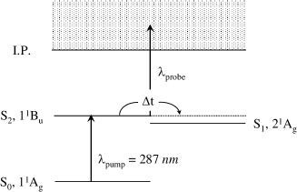
Figure 5: A femtosecond pump-probe photoionization scheme for studying excited state dynamics in all-trans decatetraene (DT). The molecule is excited to its S₂ electronic origin with a pump pulse at 287 nm (4.32 eV). Due to non-adiabatic coupling, DT undergoes rapid internal conversion to the lower lying S₁ state (3.6 eV). The excited state evolution is monitored via single photon ionization. As the ionization potential is 7.29 eV, all probe wavelengths below 417 nm permit single photon ionization of the excited state.

We consider in the following a time-resolved photoionization experiment using mass-resolved ion detection, as illustrated in Fig. 5. DT was excited to its S₂ origin and the ensuing dynamics followed by probing via single photon ionization. In DT the S₂ electronic origin is at 4.32 eV (287 nm) and the ionization potential is 7.29 eV. Hence, all probe laser wavelengths below 417 nm permit single photon ionization of the excited state. Using $\lambda_{\mathrm{pump}}=287$ nm and $\lambda_{\mathrm{probe}}=352$ nm one could therefore perform a time-resolved experiment using mass-resolved ion detection, as shown in Fig. 6. The time-resolution (pump-probe cross correlation) in these experiments was 80 fs. It can be seen in Fig. 6(a) that the parent ion C₁₀H${}_{14}^{+}$ signal rises with the laser cross-correlation and then decays with a 0.4 ps time constant. This suggests that the S₂ state lifetime is 0.4 ps. The fate of the molecule following this ultrafast internal conversion, however, cannot be discerned from these data. As mass-resolved ion signals are the observable in this experiment, one could therefore look for the appearance of any potential reaction products (e.g. fragments) following the internal conversion.

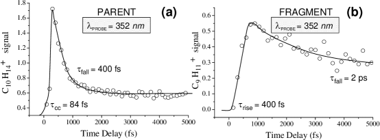
Figure 6: Time-resolved Mass Spectrometry. All-trans decatetraene (DT) was excited to its S₂ electronic origin with a fs pulse at $\lambda_{\mathrm{pump}}=287$ nm. The excited state evolution was probed via single photon ionization using a femtosecond pulse at $\lambda_{\mathrm{probe}}=352$ nm. The time-resolution in these experiments was 80 fs (0.08 ps). (a) Time-evolution of the parent ion C₁₀H${}_{14}^{+}$ signal. The parent ion signal rises with the pump laser and then decays with a single exponential time constant of 0.4 ps, suggesting that this is the lifetime of the S₂ state. The fate of the molecule subsequent to this decay is unknown from these data. (b) Time-evolution of the fragment ion C₉H${}_{11}^{+}$ signal, corresponding to methyl loss. The rise time of this fragment signal is 0.4 ps, matching the decay time of the S₂ state. This might suggest that the methyl loss channel follows directly from internal conversion to S₁. The C₉H${}_{11}^{+}$ signal subsequently decays with a time constant of about 2 ps, suggesting some further step in the excited state dynamics.

In Fig. 6(b) we present the time evolution of a fragment ion C₉H${}_{11}^{+}$ which corresponds to the loss of a methyl group from the parent molecule. The rise time of this signal is 0.4 ps, matching the decay of the parent molecule. It might be concluded from these data that the 0.4 ps decay of the S₂ state leads directly to methyl loss on the S₁ manifold. The subsequent $\sim 2$ ps decay of this signal would then be the signature of some competing process in the S₁ state, perhaps internal conversion to the S₀ ground state. In the following we will go on to show that this conclusion is, in fact, incorrect.

One might think that the specific wavelength of the photoionization laser is of little import as long as it sufficiently exceeds the ionization potential. In Fig. 7 the results of the same experiment but repeated this time using a probe laser wavelength of 235 nm are presented. As the pump laser remained invariant, the same excited state wavepacket was prepared in these two experiments. Contrasting with the 352 nm probe experiment, we see that the parent ion signal does not decay in 0.4 ps but rather remains almost constant, perhaps decaying slightly with a $\sim 1$ ps time constant. Furthermore, no daughter ion fragments were observed. These very different results seem hard to reconcile. Which probe laser wavelength gives the right answer and why? As discussed below, the time evolution of mass-resolved ion signals can be misleading.

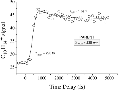
Figure 7: Time-resolved Mass Spectrometry. All-trans decatetraene (DT) was excited to its S₂ electronic origin with a fs pulse at $\lambda_{\mathrm{pump}}=287$ nm. The excited state evolution was probed via single photon ionization using a fs pulse at $\lambda_{\mathrm{probe}}=235$ nm. The time-resolution in these experiments was 290 fs (0.3 ps). The parent ion C₁₀H${}_{14}^{+}$ signal rises with the pump laser but then seems to stay almost constant with time. The modest decay observed can be fit with a single exponential time constant of $\sim 1$ ps. Note that this result is in apparent disagreement with the same experiment performed at $\lambda_{\mathrm{probe}}=352$ nm which yielding a lifetime of 0.4 ps for the S₂ state. The disagreement between these two results can be only reconciled by analyzing the time-resolved photoelectron spectrum.

The solution to this apparent paradox lies in the photoionization dynamics. Clearly the form of the parent ion signal depends strongly upon the specific photoionization dynamics and, in order to avoid misleading conclusions, must be analyzed for each specific case. The (Koopmans’) photoionization correlations of excited state electronic configurations with those of the cation play a critical role.

G TRPES: The role of electronic continua

The above pump-probe experiments on DT were repeated using TRPES rather than mass-resolved ion detection. More detailed discussions of these experimental studies of Koopmans’-type correlations with TRPES can be found in the literature [Blanchet1999, Blanchet2001, Schmitt2001]. The ultrafast internal conversion of DT provides an example of Type (I) Koopmans’ correlations, and below we’ll also discuss two experimental TRPES studies of Type (II) correlations, namely the internal conversion in the polyaromatic hydrocarbon phenanthrene, and in 1,4-diazabicyclo[2.2.2]octane (DABCO). As discussed in Section TIME-RESOLVED PHOTOELECTRON SPECTROSCOPY OF NON-ADIABATIC DYNAMICS IN POLYATOMIC MOLECULES Published in Advances in Chemical Physics, Volume 139 (ed S. A. Rice), John Wiley & Sons, Inc., Hoboken, NJ, USA. doi: 10.1002/9780470259498.ch6, Type (I) ionization correlations are defined as being the case when the neutral excited states $\alpha$ and $\beta$ in Fig. 2 correlate to different ion electronic continua, and are referred to as complementary ionization correlations. By contrast, Type (II) correlations are defined as being the case when the neutral excited states $\alpha$ and $\beta$ correlate to the same ion electronic continua, a situation labeled corresponding ionization correlations. As detailed elsewhere [Blanchet1999, Blanchet2001], the S₂ $1^{1}B_{u}$ state of DT is a singly excited configuration and has Koopmans’ correlations with the D₀ ${}^{2}B_{g}$ electronic ground state of the cation. The dipole forbidden S₁ $2^{1}A_{g}$ arises from configuration interaction between singly and doubly excited $A_{g}$ configurations and has preferential Koopmans’ correlations with the D₁ ${}^{2}A_{u}$ first excited state of the cation. These Koopmans’ correlations are illustrated in Fig. 8(a). In Fig. 8(b), we present femtosecond TRPES results on DT for 287 nm pump excitation followed by 235 nm probe laser ionization. The experimental photoelectron kinetic energy spectra reveal a rapid shift of electrons from an energetic peak ($\varepsilon_{1}$ = 2.5 eV) to a broad, structured low energy component ($\varepsilon_{2}$). The 2.5 eV band is due to ionization of S₂ into the $D_{0}$ ion state. The broad, low energy band arises from photoionization of S₁ that correlates with the $D_{1}$ ion state. Its appearance is due to population of the S₁ state by internal conversion. Integration of each photoelectron band directly reveals the S₂ to S₁ internal conversion time scale of 386$\pm$65 fs. It is important to note that these results contain more information than the overall (integrated) internal conversion time. The vibrational structure in each photoelectron band yields information about the vibrational dynamics, which promote and tune the electronic population transfer. In addition, it gives a direct view of the evolution of the ensuing intramolecular vibrational energy redistribution (IVR) in the “hot molecule” which occurs on the “dark” S₁ potential surface [Blanchet2001].

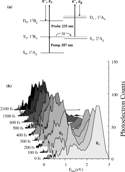
Figure 8: Time-resolved photoelectron spectra revealing vibrational and electronic dynamics during internal conversion in all trans decatetraene (DT). (a) Level scheme in DT for one-photon probe ionization. The pump laser prepares the optically bright state S₂. Due to ultrafast internal conversion, this state converts to the lower lying state S₁ with 0.7 eV of vibrational energy. The expected ionization propensity rules are shown: S${}_{2}\rightarrow D_{0}+e^{-}(\varepsilon_{1})$ and S${}_{1}\rightarrow D_{1}+e^{-}(\varepsilon_{2})$. (b) Femtosecond time-resolved photoelectron kinetic energy spectra of DT pumped at $\lambda_{\mathrm{pump}}=287$ nm and probed at $\lambda_{\mathrm{probe}}=235$ nm. There is a rapid ($\sim 400$ fs) shift in the distribution: from an energetic peak $\varepsilon_{1}$ at 2.5 eV due to photoionization of S₂ into the D₀ cation ground electronic state; to a broad, structured band $\varepsilon_{2}$ at lower energies due to photoionization of vibrationally hot S₁ into the D₁ cation first excited electronic state. These results show a disentangling of electronic population dynamics from vibrational dynamics. The structure in the low energy band reflects the vibrational dynamics in S₁.

It is instructive to compare these TRPES results with the mass-resolved ion yield experiment at the same pump and probe laser wavelengths, discussed above (see Fig. 7). The parent ion signal would be the same as integrating the photoelectron spectra in Fig. 8(b) over all electron kinetic energies. In doing so, we would sum together a decaying photoelectron band $\varepsilon_{1}$ with a growing photoelectron band $\varepsilon_{2}$, leading to a signal which is more or less constant in time and provides little information about the decay dynamics. This is the reason why the parent ion signal in Fig. 7 does not show the 0.4 ps decay that corresponds to the lifetime of the S₂ state. It provides a clear example of how the parent ion signal as a function of time can be misleading.

Why then does the time-resolved parent ion signal at 352 nm probe give the correct 0.4 ps S₂ lifetime (Fig. 6(a))? It turns out that 352 nm is just below the energy threshold for reaching the D₁ state of the cation. Therefore, upon internal conversion the formed S₁ state cannot be easily ionized via a single photon since, as discussed above, it does not have Koopmans’ correlations with the D₀ ground state of the cation. Therefore, single photon ionization probes only the decaying S₂ state which does have Koopmans’-allowed ionization into the D₀ ion ground state. Hence, the correct 0.4 ps decay is observed in the parent ion signal. The fragment ion signal has a 0.4 ps growth curve, indicating that it arises from photoionization of the S₁ state formed by internal conversion. Importantly, the observation of the fragment ion has nothing to do with a possible neutral channel dissociation in the S₁ excited state – there is none. Why then is a fragment ion observed? As both the D₀ and D₁ states of the ion are stable with respect to dissociation, it must be the case that a second probe photon is absorbed and higher lying (predissociative) states of the cation are accessed. A probe laser power study supported this point, yielding a quadratic dependence for the fragment ion and a linear dependence for the parent ion signal. But why, under invariant laser intensity, is a second probe photon absorbed only by the S₁ state and not the S₂ state? Again a consideration of the photoionization dynamics is required.

In Fig. 9, we show the time-resolved photoelectron spectrum for 352 nm probe laser ionization. Initially, the spectrum is characterized by a low energy band, $\varepsilon_{1}$ at 0.56 eV which decays with time. As indicated in Fig. 9, the $\varepsilon_{1}$ band is due to one-photon ionization of S₂ into D₀ and corresponds exactly with the 235 nm $\varepsilon_{1}$ band of Fig. 8, simply shifted to lower energy by the reduction in probe photon energy. This peak is also narrower due to the improved kinetic resolution at low energy. A broad energetic band, $\varepsilon_{2}$, ranging from 0.6 eV to 4 eV grows with time as the $\varepsilon_{1}$ band decays and therefore arises from photoionization of the formed S₁ state. The $\varepsilon_{2}$ band must, via energy conservation, arise from two-photon probe ionization. As can be seen from Fig. 9(a), due to the symmetry of the two-photon dipole operator, the ion continua accessed via two-photon ionization may also include D₀, D₃ and D₄. This explains the broad range and high kinetic energy of the photoelectrons in the $\varepsilon_{2}$ band. Integration of the $\varepsilon_{1}$ and $\varepsilon_{2}$ bands provides yet another independent confirmation of the internal conversion time scale, 377$\pm$47 fs, fully in agreement with the 235 nm probe results. It is interesting to consider why, at invariant probe laser intensity, the photoionization process switches from single photon ionization of S₂ to two-photon ionization of S₁. We note that in the both cases, the first probe photon is sufficient to ionize the excited state, and therefore the S₁ ionization is due to absorption of a second photon in the ionization continuum. This can be rationalized by a consideration of the relative rates of two competing processes: second photon absorption vs. autoionization. For the case of S₂, the photoionization correlation is with D₀ and therefore the ionization is direct. In other words, the “autoionization” is extremely rapid and second photon absorption cannot compete. For the case of S₁, the photoionization correlation is with D₁. The D₁ state, however, is energetically inaccessible and therefore the transition is most likely into Rydberg series converging on the D₁ threshold. For these to emit an electron into the open D₀ continuum channel, there must be an electronic rearrangement, for which there is a finite autoionization rate. In this case, the absorption of a second photon competes effectively with autoionization. These two-photon experiments not only confirm the one photon results, but also demonstrate the symmetry selectivity of the photoionization process itself.

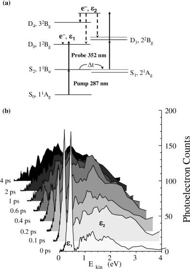
Figure 9: Time-resolved vibrational and electronic dynamics during internal conversion for all trans decatetraene (DT) pumped at $\lambda_{\mathrm{pump}}=287$ nm and probed at $\lambda_{\mathrm{probe}}=352$ nm. (a) Level scheme in DT for one- and two-photon probe ionization. The pump laser is identical to that in Fig. 8 and prepares the identical S₂ state wavepacket. The expected ionization propensity rules are: S${}_{2}\rightarrow D_{0}+e^{-}(\varepsilon_{1})$ for 1-photon ($u\leftrightarrow g$) ionization and S${}_{1}\rightarrow D_{0},D_{3},D_{4}+e^{-}(\varepsilon_{2})$ for 2-photon ($g\leftrightarrow g$) ionization. (b) Femtosecond time-resolved photoelectron kinetic energy spectra of DT pumped at 287 nm and probed at 352 nm, using both 1 and 2-photon probes. At 352 nm, the D₁ ion state is not energetically accessible from the S₁ state via a single photon transition. Confirming the results of Fig. 8, there is a rapid shift ($\sim 400$ fs) in the distribution: from $\varepsilon_{1}$ a peak at 0.4 eV due to 1-photon ionization of S₂ into the D₀ cation ground electronic state; to $\varepsilon_{2}$ a broad, structured band at higher energies (1 - 3.5 eV) due to 2-photon ionization of the vibrationally hot S₁ into the D₀ cation ground and excited electronic states. The photoionization channel switches from a 1-photon to a 2-photon process during the internal conversion indicating again that the electronic structure of the ionization continuum is selective of the evolving electronic symmetry in the neutral state.

The other limiting Koopmans’ case, Type (II), is where the one-electron correlations upon ionization correspond to the same cationic states. An example of Type (II) correlations is seen in the S₂–S₁ internal conversion in the polyaromatic hydrocarbon phenanthrene (PH), discussed in more detail elsewhere [Schmitt2001]. In the case of PH, both the S₂ and the S₁ states correlate similarly with the electronic ground state as well as the first excited state of the cation. In this experiment, PH was excited from the S₀ ${}^{1}A_{1}$ ground state to the origin of the S₂ ${}^{1}B_{2}$ state with a 282 nm (4.37 eV) femtosecond pump pulse and then ionized after a time delay $\Delta t$ using a 250 nm (4.96 eV) probe photon. The S₂ ${}^{1}B_{2}$ state rapidly internally converted to the lower lying S₁ ${}^{1}A_{1}$ state at 3.63 eV, transforming electronic into vibrational energy. In PH, both the S₂ ${}^{1}B_{2}$ and S₁ ${}^{1}A_{1}$ states can correlate with the D₀ ${}^{2}B_{1}$ ion ground state. The time-resolved photoelectron spectra for PH, shown in Fig. 10, revealed a rapidly decaying but energetically narrow peak at $\varepsilon_{1}\sim 1.5$ eV due to photoionization of the vibrationless S₂ ${}^{1}B_{2}$ state into the ionic ground state D₀ ${}^{2}B_{1}$, resulting in a decay time constant of 520$\pm$8 fs. A broad photoelectron band, centered at about $\sim 0.7$ eV, in these photoelectron spectra was due to ionization of vibrationally hot molecules in the S₁ state, formed by the S₂–S₁ internal conversion. At times t $>1500$ fs or so (i.e. after internal conversion), the photoelectron spectrum is comprised exclusively of signals due to S₁ ionization. The S₁ state itself is long lived on the time scale of the experiment. Despite the fact that Type (II) molecules present an unfavorable case for disentangling electronic from vibrational dynamics, in PH a dramatic shift in the photoelectron spectrum was seen as a function of time. This is due to the fact that PH is a rigid molecule and the S₂, S₁ and D₀ states all have similar geometries. The photoionization probabilities are therefore dominated by small $\Delta v$ transitions. Hence, the 0.74 eV vibrational energy in the populated S₁ state should be roughly conserved upon ionization into the D₀ ionic state. Small geometry changes favor conservation of vibrational energy upon ionization and thereby permit the observation of the excited state electronic population dynamics via a photoelectron kinetic energy analysis alone. In general, however, significant geometry changes will lead to overlapping photoelectron bands, hindering the disentangling of vibrational from electronic dynamics.

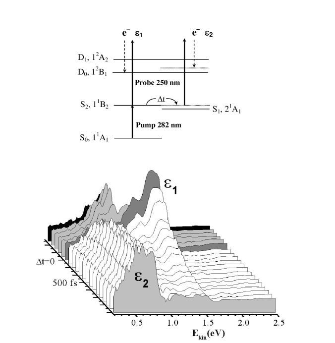
Figure 10: Energy level scheme for TRPES of phenanthrene (PH), an example of a Type (II) ionization correlation. (a) The pump laser prepares the optically bright state S₂. Due to ultrafast internal conversion, this state converts to the lower lying state S₁ with $\sim 0.74$ eV of vibrational energy. The expected corresponding Type (II) Koopmans’ correlations are shown: S${}_{2}\rightarrow D_{0}+e^{-}(\varepsilon_{1})$ and S${}_{1}\rightarrow D_{0}+e^{-}(\varepsilon_{2})$. (b) TRPES spectra of phenanthrene for a pump wavelength of $\lambda_{\mathrm{pump}}=282$ nm and a probe wavelength of $\lambda_{\mathrm{probe}}=250$ nm. The disappearance of band $\varepsilon_{1}$ at $\sim 1.5$ eV and growth of band at $\varepsilon_{2}$ at $\sim 0.5$ eV represents a direct measure of the S${}_{2}-S_{1}$ internal conversion time (520 fs). Despite the unfavourable Type(II) ionization correlations, the rigidity of this molecule allows for direct observation of the internal conversion via vibrational propensities alone.

As mentioned in Section TIME-RESOLVED PHOTOELECTRON SPECTROSCOPY OF NON-ADIABATIC DYNAMICS IN POLYATOMIC MOLECULES Published in Advances in Chemical Physics, Volume 139 (ed S. A. Rice), John Wiley & Sons, Inc., Hoboken, NJ, USA. doi: 10.1002/9780470259498.ch6, where a molecule has Type (II) ionization correlations, it might be expected that the coupled electronic states of the neutral molecule would not be resolved in the photoelectron spectrum – the rigidity of PH and the large energy gap between the S₂ and S₁ origins allowed for the resolution of the excited state dynamics in the PES, but this is by no means a general situation. In such circumstances, the measurement of time-resolved PADs (TRPADS) offers an complementary approach to unravelling the dynamics. As discussed in Section TIME-RESOLVED PHOTOELECTRON SPECTROSCOPY OF NON-ADIABATIC DYNAMICS IN POLYATOMIC MOLECULES Published in Advances in Chemical Physics, Volume 139 (ed S. A. Rice), John Wiley & Sons, Inc., Hoboken, NJ, USA. doi: 10.1002/9780470259498.ch6, the requirement that the direct product of the irreducible representations of the neutral electronic state, the transition dipole component, the ion electronic state and the free electron contains the totally symmetric representation (see Eq. (35)) means that, if the coupled electronic states are of different symmetry, the PAD will differ for the two electronic states. The evolution of the PAD can therefore be expected to provide a mechanism for unravelling the electronic dynamics. A first demonstration of a TRPADs measurement of non-adiabatically coupled electronic states was provided by Hayden and co-workers who studied the molecule 1,4-diazabicyclo[2.2.2]octane (DABCO). In this experiment, 251 nm pump pulse excited the origin of the optically bright S₂ ${}^{1}E’$ electronic state, a 3p Rydberg state centred on the nitrogen atoms [Parker1979], via a single photon excitation. The S₂ state is coupled to the lower lying optically dark S₁ ${}^{1}A^{\prime}_{1}$ state, a 3s Rydberg state centered on the nitrogen atoms, and internal conversion takes place on a $\sim 1$ ps timescale. In the experiment, it was possible to resolve the S₁ and S₂ states directly in the PES. In Fig. 11 we show PADs measured for each electronic state at different time delays, measured with a photoelectron imaging apparatus.

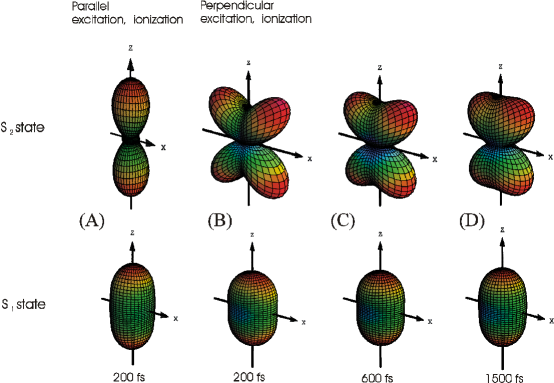
Figure 11: Time-resolved photoelectron angular distributions (PADs) from ionization of DABCO for linearly polarized pump and probe pulses.. Here the optically bright S₂ ${}^{1}E’$ state internally converts to the dark S₁ ${}^{1}A^{\prime}_{1}$ state on picosecond timescales. (A) PADs at 200 fs time delay for pump and probe polarization vector both parallel to the spectrometer axis. The difference in electronic symmetry between S₂ and S₁ leads to significant changes in the form of the PAD. (B) PADs at 200 fs time delay for pump polarization parallel and probe polarization perpendicular to the spectrometer axis, showing the effects of lab frame molecular alignment. (C) and (D) The PADs evolve as a function of time due to molecular axis rotational wavepacket dynamics. Printed with permission from C .C. Hayden, unpublished.

Although the S₂ and S₁ states of DABCO are easily resolved in the PES, due again to the rigidity of the molecule, these measurements clearly demonstrate the sensitivity of the PAD to the electronic symmetry of the excited state. Furthermore, the data displayed in Fig. 11 demonstrates the sensitivity of the PAD to the molecular axis alignment. The single-photon pump step in this experiment produces a coherent superposition of rotational states of the molecules and an anisotropic distribution of molecular axes exhibiting alignment. Comparing panels (A) and (B) in Fig. 11 we see that the PAD changes dramatically when the probe polarization is changed from being parallel to being perpendicular to the pump polarization. When the pump and probe polarizations are parallel, the LF PAD possesses cylindrical symmetry. When the pump and probe polarizations are perpendicular, cylindrical symmetry is lost, although the LF PAD exhibits reflection symmetry in the plane containing the laser polarizations. As the pump-probe time delay increases, the rotational wavepacket in the excited state dephases and the molecular axis alignment decreases accordingly. As the anisotropy of the distribution of molecular axes decreases, the PAD is also seen to become less anisotropic, and also less sensitive to the probe laser polarization direction, as discussed in Section TIME-RESOLVED PHOTOELECTRON SPECTROSCOPY OF NON-ADIABATIC DYNAMICS IN POLYATOMIC MOLECULES Published in Advances in Chemical Physics, Volume 139 (ed S. A. Rice), John Wiley & Sons, Inc., Hoboken, NJ, USA. doi: 10.1002/9780470259498.ch6.

In closing this section we note that, although the Koopmans’ picture is a simplification of the ionization dynamics, it provides a very useful zeroth order picture from which to consider the TRPES results. Any potential failure of this independent electron picture can always be experimentally tested directly through variation of the photoionization laser frequency: resonance structures should lead to variations in the form of the spectra with electron kinetic energy, although the effect of resonances is more likely to be prominent in PAD measurements, and indeed an observation of a shape resonance in para-difluorobenzene has been reported [Bellm2003, Bellm2005].

Chapter Applications

As discussed in the Introduction, a natural application of TRPES is to problems of excited state non-adiabatic dynamics. Non-adiabatic dynamics involve a breakdown of the adiabatic (Born-Oppenheimer) approximation, which assumes that electrons instantaneously follow the nuclear dynamics. This approximation is exact provided that the nuclear kinetic energy is negligible and its breakdown is therefore uniquely due to the nuclear kinetic energy operator. Spin-orbit coupling, leading to intersystem crossing, is not a non-adiabatic process in this sense: the Born-Oppenheimer states could be chosen to be the fully relativistic eigenstates and hence would be perfectly valid adiabatic states. Nevertheless, the description of intersystem crossing as a non-adiabatic process is seen in the literature and we therefore include spin-orbit coupling problems in this section. Furthermore, in this section we have chosen to include examples from work which highlight some of the most recent advances in the use of TRPES for studying molecular dynamics. These include the application of TRCIS to the study of photodissociation dynamics, as well as the use of PADs to measure molecular axis distributions, as suggested by Eq. (45). Examples are also given of the utility of TRPES for the study of excited state vibrational dynamics.

H Internal Conversion: Electronic relaxation in substituted Benzenes

Internal conversion, also referred to as spin-conserving electronic relaxation or a radiationless transition, is one of the most important non-adiabatic processes in polyatomic molecules, and is often the trigger for any ensuing photochemistry [Bixon1968, Jortner1969, Henry1973, Freed1976, Stock1997, Worth2004, Klessinger1994, Koppel1984]. As will be discussed in more detail in Section K, in order to establish rules relating molecular structure to function — a concept central to the development of molecular scale electronics — it is first necessary to develop an understanding of the relationship between molecular structure and excited state dynamics. The underlying “rules” governing these processes have yet to be fully established. A phenomenological approach to such rules involves the study of substituent effects in electronic relaxation (internal conversion) dynamics. For this reason a series of monosubstituted benzenes was studied as model compounds [Lee2002]. The focus of this work was on the first and second $\pi\pi^{\ast}$ states of these aromatic systems and on substituents which were expected to affect the electronic structure and relaxation rates of the $\pi\pi^{\ast}$ states. The photophysics of benzenes is well understood, and therefore the major purpose of this study was to establish the quantitative accuracy of the internal conversion rates determined via TRPES.

Figure 12: Molecular structures of some monosubstituted benzenes studied via TRPES in order to determine the quantitative accuracy of the extracted internal conversion rates. Three different electronic substituents were used, C=O, C=C and C$\equiv$C, leading to different state interactions. The effects of vibrational dynamics were investigated via the use of methyl group (floppier), as in $\alpha$-MeSTY and ACP, or a ring structure (more rigid), as in IND, side group additions. BZA and ACP have favourable Type (1) ionization correlations whereas STY, IND, $\alpha$-MeSTY and ACT have unfavourable Type (2) ionization correlations.

As shown in Fig. 12, six benzene derivatives were studied: benzaldehyde (BZA), styrene (STY), indene (IND), acetophenone (ACP), $\alpha$-methylstyrene ($\alpha$-MeSTY) and phenylacetylene ($\phi$ACT). This choice of substituents addressed several points: (i) the effect of the substituent on the electronic states and couplings; (ii) the effect of the substituent on the rigidity or floppiness of the MF; (iii) a comparison of Type (I) with Type (II) Koopmans’ systems; (iv) to investigate the potential effects of autoionization resonances (i.e. non-Koopmans’ behavior) on the observed dynamics. Three electronically distinct substituents were chosen: C=O, C=C and C$\equiv$C. For the C=C, potential off-axis conjugation effects with the ring in STY was contrasted with the lack of these in the C$\equiv$C of $\phi$ACT. For the heteroatomic substituent C=O, the influence of the additional n$\pi^{\ast}$ state on the $\pi\pi^{\ast}$ dynamics was investigated by comparing BZA with STY and ACP with $\alpha$-MeSTY. The effects of vibrational dynamics and densities-of-states on the electronic relaxation rates were studied via both methyl (“floppier”) and alkyl ring (“more rigid”) substitution: STY was compared with both the floppier $\alpha$-MeSTY and the much more rigid IND; BZA was compared with the floppier ACP. Both BZA and ACP have Type (I) Koopmans’ ionization correlations, the rest have Type (II) correlations, allowing for another comparison of these two cases. In order to investigate the potential effects of autoionization resonances, the ionization probe photon energy was varied ($\sim 0.4$ eV). In these systems, the form of the photoelectron spectra and the fits to the lifetime data were invariant with respect to probe laser frequency [Lee2002].

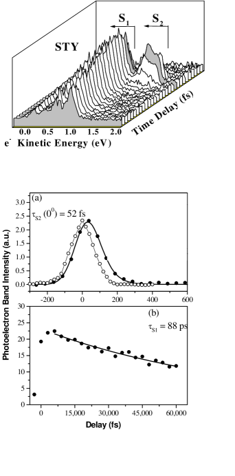
Figure 13: (top) TRPES spectra of substituted benzenes, shown here for styrene (STY) with $\lambda_{\mathrm{pump}}$ = 254.3 nm and photoionization $\lambda_{\mathrm{probe}}$ = 218.5 nm. The energetics and Koopmans’ correlations allow for assignment of the photoelectron bands to ionization of S${}_{2}(\pi\pi^{\ast})$ and S${}_{1}(\pi\pi^{\ast})$, as indicated. The S₂ state decays on ultrafast time scales. The S₁ state decays on a much longer (ps) time scale. (Bottom) (a) Time-dependent S${}_{2}(\pi\pi^{\ast})$ 0⁰ photoelectron band integral yields for STY, yielding a decay time constant of 52 fs. Open circles represent the laser cross-correlation at these wavelengths. (b) Time-dependent S${}_{1}(\pi\pi^{\ast})$ photoelectron band integral yields for STY obtained from a fit to the long time delay part of the data (not shown).

A sample TRPES spectrum, STY at $\lambda_{\mathrm{pump}}=254.3$ nm and $\lambda_{\mathrm{probe}}=218.5$ nm, is shown in Fig. 13. The S${}_{1}(\pi\pi^{\ast})$ component grows in rapidly, corresponding to the ultrafast internal conversion of the S${}_{2}(\pi\pi^{\ast})$ state. The S${}_{1}(\pi\pi^{\ast})$ component subsequently decays on a much longer picosecond time scale (not shown). It can be seen that despite STY being an unfavorable Type (II) case, the two bands are well enough resolved to allow for unambiguous separation of the two channels and determination of the sequential electronic relaxation time scales. Energy integration over each band allows for extraction of the electronic relaxation dynamics. The time-dependent S${}_{2}(\pi\pi^{\ast})$ photoelectron band integral yields for STY are also shown in Fig. 13. The open circles represent the pump-probe cross-correlation (i.e. the experimental time resolution) at these wavelengths. Integration over the S${}_{2}(\pi\pi^{\ast})$ photoelectron band is shown as the solid circles. The solid line is the best fit to the S${}_{2}(\pi\pi^{\ast})$ channel, yielding a lifetime of 52$\pm$5 fs. In Fig. 13, the time-dependent S${}_{1}(\pi\pi^{\ast})$ photoelectron band integral yields for STY are shown, obtained from a fit to the long delay part of the data, yielding a lifetime of 88$\pm$8 ps for the state S${}_{1}(\pi\pi^{\ast})$.

Figure 14: Excess vibrational energy dependence of the internal conversion rates of the first $\pi\pi^{\ast}$ state of benzene and its derivatives.

The excess vibrational energy dependence of the internal conversion rates of the first $\pi\pi^{\ast}$ state of benzene and its derivatives is shown in Fig. 14. These data suggest that the first $\pi\pi^{\ast}$ states of STY, $\alpha$-MeSTY, IND and ACT internally convert essentially via benzene ring dynamics. By contrast, the first $\pi\pi^{\ast}$ states of BZA and ACP internally convert orders of magnitude faster, indicating a completely different mechanism due to the presence of low lying n$\pi^{\ast}$ states in BZA and ACP, absent in the other systems, which lead to ultrafast intersystem crossing and the formation of triplet states. Overall, these results demonstrate that the TRPES method is well-suited to the quantitative study of electronic relaxation processes, producing direct and accurate measurements of electronic relaxation rates which are in quantitative agreement with the currently accepted understanding of aromatic photophysics [Lee2002].

I Excited state nuclear dynamics

As discussed in Section TIME-RESOLVED PHOTOELECTRON SPECTROSCOPY OF NON-ADIABATIC DYNAMICS IN POLYATOMIC MOLECULES Published in Advances in Chemical Physics, Volume 139 (ed S. A. Rice), John Wiley & Sons, Inc., Hoboken, NJ, USA. doi: 10.1002/9780470259498.ch6, TRPES is sensitive to vibrational and rotational dynamics, as well as electronic dynamics. In this section, we will give examples of the use of TRPES to the study of intramolecular vibrational energy redistribution (IVR), and the use of time-resolved PAD measurements as a probe of rotational dynamics.

A problem central to chemical reaction dynamics is that of IVR [Felker1995, Keske2000], the flow of energy between zeroth-order vibrational modes. Indeed, IVR generally accompanies (and mediates) non-adiabatic dynamics such as internal conversion and isomerization. The description of separated rigid rotational and normal-mode vibrational motions employed in Section B and Section TIME-RESOLVED PHOTOELECTRON SPECTROSCOPY OF NON-ADIABATIC DYNAMICS IN POLYATOMIC MOLECULES Published in Advances in Chemical Physics, Volume 139 (ed S. A. Rice), John Wiley & Sons, Inc., Hoboken, NJ, USA. doi: 10.1002/9780470259498.ch6 provides an adequate description only in regions of low state density. As the state density increases, the vibrational dynamics become “dissipative” as normal-mode vibrations become mixed and energy flows between these zeroth-order states. Much work has been undertaken studying IVR using e.g. fluroscence techniques [Moss1993, Felker1995, Keske2000]. However, such techniques generally monitor flow of energy out of the initially excited vibrational states, but do not directly observe the optically dark “bath” vibrational modes into which vibrational energy flows. TRPES provides a window to these dark states, allowing for direct monitoring of IVR in molecules due to the Franck-Condon correlations described in Section TIME-RESOLVED PHOTOELECTRON SPECTROSCOPY OF NON-ADIABATIC DYNAMICS IN POLYATOMIC MOLECULES Published in Advances in Chemical Physics, Volume 139 (ed S. A. Rice), John Wiley & Sons, Inc., Hoboken, NJ, USA. doi: 10.1002/9780470259498.ch6.

Reid and co-workers reported a picosecond TRPES study of IVR in the electronically excited S₁ state of para-fluorotoluene [King2005]. By selective excitation of specific vibrational modes in S₁ and measuring the evolution of the PES as a function of time delay, information regarding vibrational population dynamics was obtained. Analysis of this TRPES data also employed high resolution PES data and required a detailed understanding of the Franck-Condon factors for ionization. Reid and co-workers were able to measure the rates of IVR for the the initially prepared $7^{1}$, $8^{1}$ and $11^{1}$ vibrational states (using Mulliken notation) of the first electronically excited state S₁ of para-fluorotoluene [King2005]. By selective population of vibrational states in S₁ it is possible to use TRPES to test for vibrational mode-specificity in IVR, as well as varying the excess vibrational energy. In Fig. 15 example TRPES data is shown for excitation of the $7^{1}$ mode of para-fluorotoluene, corresponding to one quanta of excitation in the C–F stretching mode, and representing 1230 cm^-1 vibrational energy in S₁. The evolution of the PES shown in Fig. 15, and the disappearance of resolved structure at long time delays is a direct measure of the IVR of energy out of the C–F stretching mode and into other modes of the molecule. By analysing spectra such as those in Fig. 15 in terms of the population in the initially prepared state compared to the populations in all other “dark” modes, the rate of IVR may be extracted. An example of such an analysis is shown in Fig. 16.

Figure 15: TRPES of the S₁ state of para-fluortoluene prepared in the $7^{1}$ state, i.e. with one quanta of excitation in the C–F stretching mode. At early times, the PES contains a well resolved Franck-Condon progression corresponding to ionization of the localized C–F stretching mode. At later times, the onset of IVR obscures the PES as many more vibrational modes become populated. Reproduced with permission from ref. [King2005].

Figure 16: Ratio of the population of the initially prepared vibrational state to the population of the “dark” vibrational states populated through IVR for the data shown in Fig. 15. Reproduced with permission from ref. [King2005].

In a second example of the utility of TRPES for the study of vibrational dynamics, Reid and co-workers studied the dynamics associated with a Fermi resonance between two near-degenerate vibrational modes in the S₁ state of toluene [Hammond2006]. In this study, the pump pulse prepared a coherent superposition of the $6a^{1}$ state, corresponding to one quanta of vibrational excitation in the totally symmetric ring breathing mode, and the $10b^{1}6b^{1}$ state, corresponding to one quanta in the CH₃ wagging mode ($10b$) and one quanta in the C–H out-of-plane bending mode ($16b$). The anharmonic coupling between these two states gives rise to an oscillation in the form of the PES, as shown in Fig. 17, the timescale of which corresponds to the energy separation of the two vibrational modes.

Figure 17: (Top) Photoelectron spectra following preparation of the $6a^{1}+10b^{1}6b^{1}$ Fermi resonance at 457 cm^-1 in the S₁ state of toluene with a 1 ps pump pulse. PES are shown as a function of time delay between the pump pulse and a 1 ps probe pulse. (Bottom) Fits to the oscillation of the PES according to two different models of the data shown in the top panel showing clearly a period of oscillation of $\sim 6$ ps, corresponding to the energy separation of the two vibrational states comprising the wavepacket. For more detail see ref. [Hammond2006]. Reproduced with permission from ref. [Hammond2006].

As discussed in Section TIME-RESOLVED PHOTOELECTRON SPECTROSCOPY OF NON-ADIABATIC DYNAMICS IN POLYATOMIC MOLECULES Published in Advances in Chemical Physics, Volume 139 (ed S. A. Rice), John Wiley & Sons, Inc., Hoboken, NJ, USA. doi: 10.1002/9780470259498.ch6 time-resolved PAD (TRPAD) measurements are sensitive to molecular rotational motion by virtue of their geometric dependence upon the molecular axis distribution in the LF. An elegant experimental demonstration of this has been performed by Suzuki and co-workers who measured the PAD temporal evolution from excited state pyrazine [Tsubouchi2001]. In these experiments, the origin of the S₁ electronic state of pyrazine was excited by a pump pulse at 323 nm, and subsequently probed by a time delayed probe pulse via a two photon ionization. In this energy region, the excited state dynamics of pyrazine involve a well studied intersystem crossing caused by strong spin-orbit coupling of the S₁ $B_{3u}(n\pi^{\ast})$ state with a manifold of triplet states, denoted T₁, resulting in a complex energy spectrum [McDonald1981, Knee1985, Lorincz1985, Felker1986]. While earlier studies focussed on the monitoring of fluorescence from the S₁ state, this work directly measured the S₁ decay and the T₁ formation via TRPES and TRPAD measurements. Two photon ionization in these experiments proceeded via 3s and 3p_z Rydberg states of the neutral, producing well resolved bands attributable to the S₁ and T₁ states (see Fig. 18).

Figure 18: (a) Inverse Abel transformed photoelectron image showing the lab frame PAD for ionization of pyrazine with a pump pulse at 323 nm and a probe pulse at 401 nm. The laser pulses had parallel linear polarizations and a temporal separation of 30 ps. The outer two rings correspond to two photon ionization of the S₁ electronic state via3s and 3p Rydberg states, and the inner ring corresponds to two-photon ionization of the triplet state manifold T₁ in the neutral formed by inter-system crossing from the S₁ state. (b) Time-dependence of the angle-integrated signals in (a). (c) Time-dependence of the PAD anisotropy for the 3 signals in (b) as monitored by the ratio of the PAD parameters $\beta_{20}/\beta_{00}$ from a fit to an expansion in spherical harmonics, Eq. (42).

In these experiments, the pump and probe pulse were linearly polarized with their electric fields vectors mutually parallel. The pump pulse created an initially aligned $\cos^{2}\theta$ distribution of principle molecular axes, with $\theta$ the polar angle between the principle molecular axis and the laser field polarization. This initially prepared rotational wavepacket subsequently evolved with time, and the ionization yield (shown in panel (b) of Fig. 18) from the singlet state directly reflected this wavepacket evolution, exhibiting the expected rotational recurrence behaviour of a near oblate symmetric top [Felker1995, Felker1994, Felker1992, Felker1992a, Baskin1987, Baskin1986]. The sensitivity of the photoelectron yield to the molecular axis alignment arises due to the well defined molecular frame direction of the transition dipole momement for excitation of the intermediate Rydberg states in the probe step – the 3p${}_{z}\leftarrow$S₁ and the 3p${}_{z}\leftarrow$S₁ transitions being perpendicular and parallel to the principle molecular axis respectively, resulting in the opposite (“out of phase”) behaviours in the black and red lines showin in panel (b) of Fig. 18. Interestingly, the rotational coherence is also directly observed in the signal representing the formation of the T₁ manifold (blue line in Fig. 18), demonstrating that rotational coherence is (perhaps partially) preserved upon internal conversion [Tsubouchi2004, Suzuki2006]. Additionally, the PAD also reflected the wavepacket evolution with the time dependence of the value of $\beta_{20}/\beta_{00}$ mapping the rotational recurrence behaviour, as shown in panel (c) of Fig. 18. In this case the different dependence upon molecular axis alignment of the LF PAD for ionization via the 3s vs. the 3p_z Rydberg states reflects the different MF PADs for ionization of these two Rydberg states. These measurements demonstrate the utility of TRPAD measurements as a probe of rotational dynamics. Such measurements are sensitive to vibration-rotation coupling [Reid1999, Althorpe2000, Seideman2000a, Althorpe1999].

J Excited State Intramolecular Proton Transfer

Excited state intramolecular proton transfer (ESIPT) processes are important for both practical and fundamental reasons. o-Hydroxybenzaldehyde (OHBA) is the simplest aromatic molecule displaying ESIPT and serves as a model system for comparison with theory. TRPES was used to study ESIPT in OHBA, monodeuterated ODBA and an analogous two-ring system hydroxyacetonaphtone (HAN) as a function of pump laser wavelength, tuning over the entire enol S${}_{1}(\pi\pi^{\ast})$ absorption band of these molecules [Lochbrunner2000a, Lochbrunner2001]. The experimental scheme is depicted in Fig. 19, showing energetics for the case of OHBA. Excitation with a tuneable pump laser h$\nu_{\mathrm{pump}}$ forms the enol tautomer in the S${}_{1}(\pi\pi^{\ast})$ state. ESIPT leads to ultrafast population transfer from the S₁ enol to the S₁ keto tautomer. On a longer time scale, the S₁ keto population decays via internal conversion to the ground state. Both the enol and keto excited state populations are probed by photoionization with a probe laser h$\nu_{\mathrm{probe}}$, producing the two photoelectron bands $\varepsilon_{1}$ and $\varepsilon_{2}$.

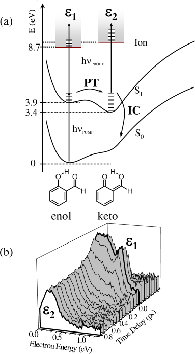
Figure 19: (Top) Energetics for excited state intramolecular proton transfer (ESIPT) in OHBA, showing the enol and keto forms. Excitation with a pump laser forms the enol tautomer in the S${}_{1}(\pi\pi^{\ast})$ state. ESIPT leads to ultrafast population transfer from the S₁ enol to the S₁ keto tautomer. On a longer time scale, the keto S₁ population decays via internal conversion to the keto ground state. Both the enol and keto excited state populations are probed via TRPES, producing the two photoelectron bands $\varepsilon_{1}$ and $\varepsilon_{2}$. (Bottom) TRPES spectra of OHBA at an excitation wavelength of 326 nm and a probe wavelength of 207 nm. Two photoelectron bands were observed: $\varepsilon_{1}$ due to ionization of the S₁ enol, and $\varepsilon_{2}$ due to ionization of the S₁ keto. Band $\varepsilon_{1}$ was observed only when the pump and probe laser beams overlapped in time, indicating a sub-50 fs timescale for the proton transfer. Band $\varepsilon_{2}$ displayed a pump wavelength dependent lifetime in the picosecond range corresponding to the energy dependent internal conversion rate of the dark S₁ keto state formed by the proton transfer.

In Fig. 19 are TRPES spectra of OHBA at an excitation wavelength of 326 nm. Two photoelectron bands $\varepsilon_{1}$ and $\varepsilon_{2}$ with distinct dynamics were observed. Band $\varepsilon_{1}$ is due to photoionization of the initially populated S₁ enol tautomer, and band $\varepsilon_{2}$ is due to the photoionization of the S₁ keto tautomer. The decay of band $\varepsilon_{1}$ yields an estimated upper limit of 50 fs for the lifetime of the S₁ enol tautomer. Proton transfer reactions often proceed via tunneling of the proton through a barrier. Deuteration of the transferred proton should then significantly prolong the lifetime of the S₁ enol tautomer. In experiments with ODBA, an isotope effect was not observed – i.e. the ESIPT reaction was again complete within the laser cross-correlation.

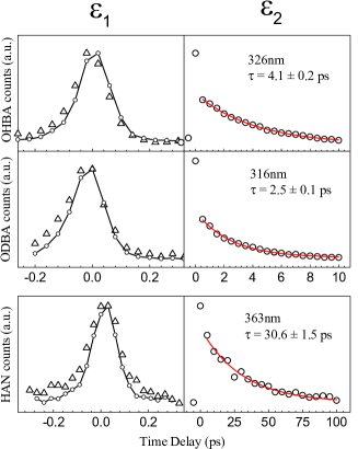
Figure 20: Integrated signals $\varepsilon_{1}$ and $\varepsilon_{2}$ for OHBA (top), ODBA (middle), and HAN (bottom) plotted as a function of the time delay at the indicated excitation wavelength. Note the change in ordinate time scales. Signal $\varepsilon_{1}$ always followed the laser cross-correlation, indicating a rapid proton transfer reaction. The decay of signal $\varepsilon_{2}$ was fitted via single exponential decay, yielding the time constant for internal conversion of the S₁ keto state in each molecule.

In Fig. 20 are examples of fits to OHBA at 326 nm, ODBA at 316 nm, and HAN at 363 nm. The proton transfer rates for all three molecules were sub-50 fs over their entire S₁ enol absorption bands. It was concluded that the barrier in the OH stretch coordinate must be very small or non-existent. This interpretation is consistent with ab initio calculations which predict no barrier for the proton transfer [Sobolewski1994, Sobolewski1999]. An estimate of the corresponding reaction rate using an instanton calculation, which takes into account the multi-mode character of proton transfer, resulted in S₁ enol lifetimes of $\sim 20$ fs for the transfer of a proton and $<$50 fs for the transfer of a deuteron when the barrier was lowered to 2.4 kcal/mol [Lochbrunner2000a, Lochbrunner2001]. This value was considered to be an upper limit for the proton transfer barrier.

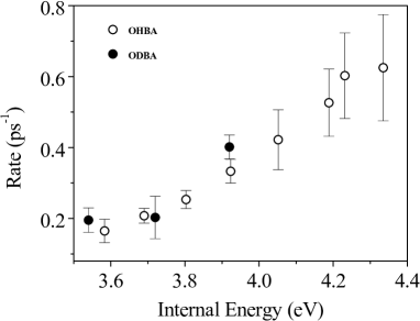
Figure 21: Internal conversion rates of the S₁ keto state of OHBA (open circles) and ODBA (filled circles), determined by single exponential fits to the $\varepsilon_{2}$ band decay. Both show a monotonic increase in rate as a function of the excitation energy, but without a significant isotope effect.

As is common in TRPES, these spectra also give insights into the dynamics on the “dark” S₁ keto state. The picosecond decay of band $\varepsilon_{2}$ corresponds to S₁ keto internal conversion to the ground state. The wavelength-dependent S₁ keto internal conversion rates for OHBA and ODBA shown in Fig. 21 revealed no significant isotope effect. Interestingly, the measured internal conversion rates for OHBA/ODBA are very fast (1.6–6 ps over the range 286–346 nm) considering the large energy gap of 3.2 eV between the ground and excited state. One possibility is that fast internal conversion in such systems is due to an efficient conical intersection involving a $\pi\pi^{\ast}$ state with a $\pi\sigma^{\ast}$ via large amplitude hydroxy H-atom motion [Sobolewski1994, Sobolewski1999]. However, the observed absence of an isotope effect on S₁ keto internal conversion rates in ODBA does not support this mechanism. A clue is found in the comparison with internal conversion rates of OHBA/ODBA with the larger HAN, shown in Fig. 20. HAN has both a smaller S₁–S₀ energy gap and a higher density of states, leading to the expectation that its internal conversion rate should be faster than that of OHBA. Surprisingly, it is about ten times slower, indicating that some other effect must be operative. A major difference between the two molecules is the position of a n$\pi^{\ast}$ state, which is almost isoenergetic with the $\pi\pi^{\ast}$ state in OHBA, but more than 0.5 eV higher in HAN. The coupling of the $\pi\pi^{\ast}$ and n$\pi^{\ast}$ states, mediated by out-of-plane vibrations, greatly increases the internal conversion rate in OHBA. The local mode character of the OH out-of-plane bending vibration makes this mode inefficient for the coupling of the n$\pi^{\ast}$ and $\pi\pi^{\ast}$ states. As a result, the bending modes of the aromatic ring dominate this interaction, which explains the absence of an isotope effect [Lochbrunner2000a, Lochbrunner2001]. This example serves to illustrate how TRPES can be used to study the dynamics of biologically relevant processes such as ESIPT and that it reveals details of both the proton transfer step and the subsequent dynamics in the “dark” state formed after the proton transfer.

K Dynamics of Molecular Electronic Switches

The burgeoning area of active molecular electronics involves the use of molecules or molecular assemblies acting as switches, transistors or modulators. A central theme is that structural rearrangement processes such as isomerization should lead to changes in either optical or electrical properties, generating the desired effect. It is often proposed that these structural rearrangements be induced via electronic excitation. The rational design of active molecular electronic devices must include a detailed consideration of the dynamics of the “switching” process for several reasons. Foremost is that activation of the device (e.g. by a photon) must indeed lead to the desired change in optical or electrical properties and therefore this basic mechanism must be present. Two other issues, however, are of great practical significance. The efficiency of the molecular electronic process is an critical element because excited organic molecules often have a variety of complex decay paths that compete with the desired process. The efficiency of a device can be defined simply as the rate of the desired process divided by the sum of the rates of all competing processes. As certain of these competing processes can occur on ultrafast time scales (e.g. dissipation, dissociation), the rate of the desired process must be very fast indeed, even if the required overall response is slow. A directly related issue is that of stability. A molecular modulator that operates at 1 GHz and lasts for three years must “switch” $\sim 10^{17}$ times without malfunction. The quantum yields of any “harmful” processes must therefore be exceedingly small. Unfortunately, excited organic molecules have a number of destructive decay pathways such as photodissociation and triplet formation (often leading to reaction). The relative rates and quantum yields of these processes as well as their dependence on substituent and environmental effects, will be critical elements in the design of efficient, stable active molecular devices. Trans-azobenzene is often considered the canonical molecular switch and its photoisomerization is the basis for numerous functional materials [Rau1990]. Azobenzene provides an important example for the study of the dynamics of Molecular Electronic switches via TRPES [Schultz2003].

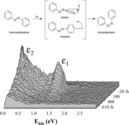
Figure 22: (Top) Photoisomerization dynamics of trans- to cis-azobenzene, indicating torsional and inversion pathways. (Bottom). TRPES spectra of trans-azobenzene excited at 330 nm and probed at 207 nm. Two photoelectron bands $\varepsilon_{1}$ and $\varepsilon_{2}$ were observed, having identical laser-limited risetimes but differing decay rates ($\tau_{1}=130$ fs, $\tau_{2}=410$ fs) and, importantly differing Koopmans’ ionization correlations. These results indicate that there is a previously unrecognized $\pi\pi^{\ast}$ state, S₃ (centered on the aromatic rings), involved in the dynamics.

Despite great interest in azobenzene photophysics, the basic photoisomerization mechanism remains disputed [Tamai2000]: in contrast to the expectations of Kasha’s rule, the isomerization quantum yield decreases rather than increases with increasing photon energy. In Fig. 22, the two possible isomerization channels, proceeding via either a planar pathway (inversion) or a non-planar, twisted pathway (torsion) are shown. Previous studies determined that isomerization in the first excited state S₁ state proceeds along the inversion coordinate [Rau1990]. The second excited state S${}_{2}(\pi\pi^{\ast}_{\mathrm{N=N}})$ is generally thought to be the N=N analogue of the C=C $\pi\pi^{\ast}$-state in stilbene and that, somehow, motion along the torsional coordinate in S${}_{2}(\pi\pi^{\ast}_{\mathrm{N=N}})$ is responsible for the observed reduction in isomerization yield. Time-resolved studies suggested that photoisomerization proceeds via the inversion coordinate in S₁ [Rau1990]. The role of the torsional isomerization pathway remains controversial. Theoretical studies have supported both torsion and inversion pathways but disagreed on the states involved in the excited state relaxation. Any successful model considering $\pi\pi^{\ast}$ state relaxation in AZ must address three puzzling features [Schultz2003]: (A) The violation of Kasha’s rule, i.e. $\Phi_{\mathrm{isom}}\sim 25\%$ for S${}_{1}(\mathrm{n}\pi^{\ast})$ but drops to $\Phi_{\mathrm{isom}}\sim 12\%$ for the higher lying $\pi\pi^{\ast}$ state(s); (B) Inhibition of the torsional coordinate in sterically restrained AZ increases $\Phi_{\mathrm{isom}}$ of the $\pi\pi^{\ast}$ states to a level identical to that observed for S₁ photoexcitation; (C) The observation of efficient relaxation of S${}_{2}(\pi\pi^{\ast})$ to the S₁ state via planar geometries.

In Fig. 22 a time-resolved photoelectron spectrum for excitation of AZ to the origin of its S${}_{2}(\pi\pi^{\ast}_{\mathrm{N=N}})$ state is shown. Two photoelectron bands $\varepsilon_{1}$ and $\varepsilon_{2}$ with differing lifetimes and differing Koopmans’ correlations were observed. Due to these two differences, the $\varepsilon_{1}$ and $\varepsilon_{2}$ bands must be understood as arising from the ionization of two different electronic states. Furthermore, as both bands rise within the laser cross-correlation, they are due to direct photoexcitation from S₀ and not to secondary processes. Therefore, in order to account for different lifetimes, different Koopmans’ correlations and simultaneous excitation from S₀, the existence of an additional state, labeled S${}_{3}(\pi\pi^{\ast}_{\phi})$, which overlaps spectroscopically with S${}_{2}(\pi\pi^{\ast}_{\mathrm{N=N}})$ must be invoked. According to the Koopmans’ analysis (based upon assignment of the photoelectron bands) and to high level, large active space CASSCF calculations, this new state S${}_{3}(\pi\pi^{\ast}_{\phi})$ corresponds to $\pi\pi^{\ast}$ excitation of the phenyl rings [Schultz2003], as opposed to the S${}_{2}(\pi\pi^{\ast}_{\mathrm{N=N}})$ state where excitation is localized on the N=N bond. Therefore, $\pi\pi^{\ast}$-excitation in the phenyl rings does not directly “break” the N=N bond and leads to reduced isomerization quantum yields.

A new model for AZ photophysics was proposed as a result of these TRPES studies. The S${}_{2}(\pi\pi^{\ast}_{\mathrm{N=N}})$ state internally converts to S₁ in a planar geometry, explaining puzzle (C) above. The subsequent relaxation of S₁ does indeed follow Kasha’s rule and yields $\Phi_{\mathrm{isom}}\sim 25\%$ for the population originating from S${}_{2}(\pi\pi^{\ast}_{\mathrm{N=N}})$. Different dynamics are observed in the TRPES experiments for the S${}_{3}(\pi\pi^{\ast}_{\phi})$ state, indicating a different relaxation pathway. To explain puzzle (A), relaxation of S${}_{3}(\pi\pi^{\ast}_{\phi})$ with reduced isomerization must be assumed: the ring-localized character of S${}_{3}(\pi\pi^{\ast}_{\phi})$ suggests a relaxation pathway involving phenyl-ring dynamics. This could involve torsion and lead directly to the trans-AZ ground state – explaining both puzzles (A) and (B). Ab initio Molecular Dynamics (AIMD) simulations [Schultz2003] starting from the Franck-Condon geometry in S${}_{2}(\pi\pi^{\ast}_{\mathrm{N=N}})$ agree with result (C) and predict that the molecule quickly ($<50$ fs) samples geometries near conical intersections while still in a planar geometry, with no evidence for torsion or inversion. For S₁, the AIMD simulations predict that a conical intersection involving inversion is approached within 50 fs [Schultz2003]. This mechanism differs greatly from that of all earlier models in that those always assumed that only a single bright state, S${}_{2}(\pi\pi^{\ast}_{\mathrm{N=N}})$, exists in this wavelength region. This example shows how TRPES can be used to study competing electronic relaxation pathways in a model molecular switch, revealing hidden yet important electronic states that can be very hard to discern via conventional means.

L Photodissociation Dynamics

From the point of view of chemical reaction dynamics, the most interesting case is that of unbound excited states or excited states coupled to a dissociative continuum – i.e. photodissociation dynamics. The dissociative electronically excited states of polyatomic molecules can exhibit very complex dynamics, usually involving non-adiabatic processes. TRPES and TRCIS may be used to study the complex dissociation dynamics of neutral polyatomic molecules, and below we’ll give two examples of dissociative molecular systems that have been studied by these approaches, NO₂ and (NO)₂.

TRCIS was first applied to dissociative multiphoton ionization of NO₂ at 375.3 nm [Davies1999]. This was identified as a three-photon transition to a repulsive surface correlating with NO(C ${}^{2}\Pi$)+O(${}^{3}P$) fragments. The NO(C) was subsequently ionizing by a single photon, yielding NO⁺(X${}^{1}\Sigma^{+}$)+e^-.

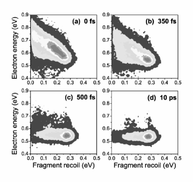
Figure 23: Time-Resolved Coincidence-Imaging Spectroscopy (TRCIS) of dissociative multiphoton ionization processes in NO₂ using  100 fs laser pulses at 375.3 nm, using energy-energy correlations. The two dimensional maps show, at time delays of 0 fs, 350 fs, 500 fs and 10 ps, the correlation between the photoelectron kinetic energy (abscissa) and NO photofragment recoil energy (ordinate). The intensity distributions change from a negative correlation at early times to uncorrelated at later times, yielding information about the molecule as it dissociates. Reproduced with permission from ref. [Davies1999]

As an illustration of the multiply differential information obtained via TRCIS, energy-energy correlations plotting photoelectron kinetic energy vs. NO(C) photofragment kinetic energy, as a function of time, are shown in Fig. 23. At early times, 0 fs and 350 fs, there is a negative correlation between electron and fragment recoil energy. This is the form expected for a molecule in the process of dissociating where there is a trade-off between ionization energy and fragment recoil energy. At longer time delays, 500 fs and 10 ps, the NO(C) fragment is no longer recoiling from the O atom – it is a free particle – and the photoelectron spectrum obtained is simply that of free NO(C) and, hence, the negative correlation vanishes [Davies1999]. By measuring the angle of recoil of both photoelectron and photofragment in coincidence, the PAD may be transformed into the RF at each time delay [Davies2000]. In Fig. 24, the time-resolved RF PADs are shown for the case of photofragments ejected parallel to the laser polarization axis. It can be seen that at early times, 0 and 350 fs, the PAD is highly asymmetric. The breaking of forward-backward symmetry in the RF originates from NO(C) polarization due to the presence of the O atom from which it is recoiling. At longer times, 1 ps and 10 ps, this forward-backward asymmetry vanishes, as the NO(C) becomes a free particle. This once again shows the power of TRCIS in obtaining highly detailed information about molecules in the process of dissociating.

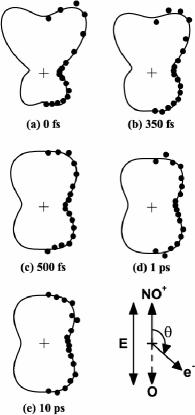
Figure 24: Coincidence-Imaging Spectroscopy of dissociative multiphoton ionization processes in NO₂ with $\sim 100$ fs laser pulses at 375.3 nm, using angle-angle correlations. The polar plots show, at time delays of 0 fs, 350 fs, 500 fs, 1 ps and 10 ps, the angular correlation between the ejected electron and NO photofragment when the latter is ejected parallel to the laser field polarization vector. The intensity distributions change from a forward-backward asymmetric distribution at early times to a symmetric angular distribution at later times, yielding detailed information about the molecule as it dissociates. Reproduced with permission from ref. [Davies2000]

A second illustrative example of the utility of TRPES and TRCIS for studying complex molecular photodissociation dynamics which involve multiple electronic state is the case of the weakly bound cis-planar $C_{2v}$ nitric oxide dimer [Blanchet1998a]. The weak (D₀ = 710 cm${}^{-1})$ ${}^{1}A_{1}$ ground state covalent bond is formed by the pairing of two singly occupied $\pi^{\ast}$ orbitals, one from each NO(X${}^{2}\Pi)$ monomer. The very intense UV absorption spectrum of the NO dimer appears broad and featureless and spans a 190–240 nm range, with a maximum at $\sim 205$ nm. This transition was assigned as ${}^{1}B_{2}\leftarrow{}^{1}A_{1}$ and therefore has a transition dipole along the N–N bond direction (with $B_{2}$ symmetry). Recent ab initio studies of the excited electronic states of the dimer revealed a complex set of interactions between two very strongly absorbing states of mixed valence/Rydberg character that play a central role in the photodissociation dynamics [Levchenko2006]. As we shall see from the following measurements, these “diabatic” states are roughly comprised of a diffuse 3p_y Rydberg function (the $y$-axis is along the N–N bond) and a localized valence function which has charge transfer character and therefore carries most of the oscillator strength in the Franck-Condon region, as the oscillator strengths are much too high for a pure Rydberg state [Levchenko2006]. At 210 nm excitation one product channel is dominant:

$$(\mathrm{NO})_{2}^{\ast}\rightarrow\mathrm{NO}(\mathrm{A}^{2}\Sigma^{+},v,J)+\mathrm{NO}(\mathrm{X}^{2}\Pi,v^{\prime},J^{\prime}).$$ (55)

The fragment excited state $\mathrm{NO}(\mathrm{A}^{2}\Sigma^{+})$ is a molecular 3s Rydberg state, and we shall refer to this as NO(A, 3s). The observed NO(A, 3s) product state distributions supported the notion of a planar dissociation involving restricted intramolecular vibrational energy redistribution (IVR) [Demyanenko2002]. A scheme for studying NO dimer photodissociation dynamics via TRPES is depicted in Fig. 25. The NO(A, 3s)+NO(X) product elimination channel, its scalar and vector properties and its evolution on the femtosecond time scale have been discussed in a number of recent publications (see ref. [Levchenko2006] and references therein).

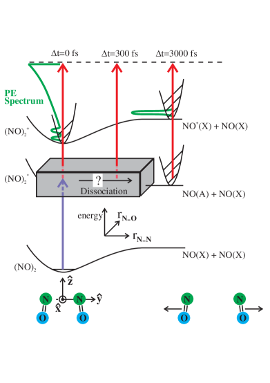
Figure 25: A femtosecond TRPES scheme for studying NO dimer photodissociation. A UV pump pulse creates the excited state (NO)${}_{2}^{\ast}$. Its subsequent evolution is monitored all the way from initial excitation to final product emission via a UV probe pulse, projecting the wavepacket onto the ionization continuum. The resulting photoelectron spectrum, reflecting vibrational and electronic changes during dissociation, is depicted in green.

The first TRPES study of NO dimer photodissociation at 210 nm excitation (and 287 nm probe) showed that the decaying (NO)${}_{2}^{+}$ parent ion signal disappeared more rapidly (when fit to a single exponential decay of 0.3 ps) than the NO(A, 3s) state product signal appeared to rise (when fit to a single exponential growth of 0.7 ps) [Blanchet1998a]. This result shows once again that the time dependence of the parent ion signal alone can be misleading. Due to its Rydberg character, the NO(A 3s, $v$, $J$) products produced a single sharp peak in the photoelectron spectrum, due to the well known NO(A${}^{2}\Sigma^{+}$, $v$, $J$) $\rightarrow$ NO⁺(X, ${}^{1}\Sigma^{+}$, $v$) ionizing transition which has predominantly $\Delta v=0$. The dissociation dynamics was interpreted in terms of a two step sequential process involving an unknown intermediate configuration. Subsequent femtosecond time-resolved ion and photoelectron imaging studies further considered the dissociation dynamics of the NO dimer [Tsubouchi2003, Tsubouchi2003a, Tsubouchi2005]. These reported the observation that both the decaying NO dimer cation signal and the rising NO(A) photoelectron signal could be fit using single exponential functions. Furthermore, the emerging NO(A, 3s) photoelectron peak changed shape and shifted in energy (by 15-20 meV) at early times. This was taken as evidence for formation of a dimer 3s Rydberg state which was expected to correlate directly to NO(A, 3s) + NO(X) products. It was argued that when the shifting of this peak is taken into consideration, the decay of the parent signal and the rise of the product signal could be fit with the same single exponential time constant, suggesting no need for an intermediate configuration.

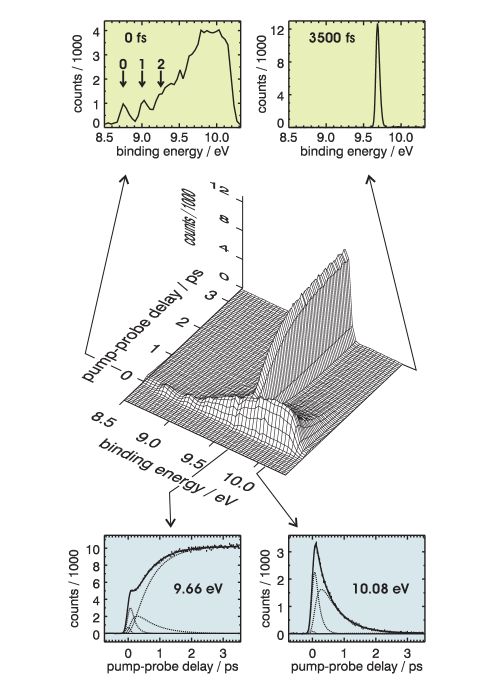
Figure 26: TRPES of NO dimer photodissociation at 210nm excitation [Gessner2006]. The broad, decaying spectrum apparent at early times is due to photoionization of the dissociating excited parent molecule. The sharp peak emerging with time is due to growth of the free NO(A, 3s) products. These 2D data are globally fit at all energies and time delays simultaneously. The green inserts (top) are 1D cuts along the energy axis, showing photoelectron spectra at two selected time delays. The blue inserts (bottom) are 1D cuts along the time axis, showing the evolution of the photoelectron intensity at two selected binding energies. The solid lines in the blue graphs are from the 2D fits to the sequential two-step dissociation model discussed in the text. The dashed lines are the respective initial, intermediate and final state signal components.

Recently, the photodissociation dynamics of the NO dimer was reinvestigated using a high sensitivity magnetic bottle technique combined with Time-Resolved Coincidence Imaging Spectroscopy (TRCIS, discussed below) [Gessner2006]. In Fig. 26 we show a magnetic bottle TRPES spectrum of (NO)₂ photodissociation. At $\Delta t=0$, a broad spectrum due to photoionization of (NO)${}_{2}^{\ast}$ shows two resolved vibrational peaks assigned to 0 and 1 quanta of the cation N=O stretch mode ($\nu_{1}$). The $\nu_{1}=2$ peaks merges with a broad, intense Franck-Condon dissociative continuum. At long times ($\Delta t=3500$ fs), a sharp photoelectron spectrum of the free NO(A, 3s) product is seen. The 10.08 eV band shows the decay of the (NO)${}_{2}^{\ast}$ excited state. The 9.66 eV band shows both the decay of (NO)${}_{2}^{\ast}$ and the growth of free NO(A, 3s) product. It is not possible to fit these via single exponential kinetics. However, these 2D data are fit very accurately at all photoelectron energies and all time delays simultaneously by a two-step sequential model, implying that an initial bright state (NO)${}_{2}^{\ast}$ evolves to an intermediate configuration $\mathrm{(NO)}_{2}^{\ast{\dagger}}$ which itself subsequently decays to yield free NO(A, 3s) products [Gessner2006]

$$(\mathrm{NO})_{2}^{\ast}\rightarrow(\mathrm{NO})_{2}^{\ast{\dagger}}\rightarrow~{}\mathrm{NO}(\mathrm{A},\mathrm{3s})+\mathrm{NO}(\mathrm{X})$$ (56)

The requirement for a sequential model is seen in the 9.66 eV photoelectron band, showing NO(A, 3s) product growth. The delayed rise of the free NO(A, 3s) signal simply cannot be fit by a single exponential decay followed by single exponential growth with the same time constant. The 10.08 eV dissociative ionization band, dominant at early times, is revealing of (NO)${}_{2}^{\ast}$ configurations preceding dissociation. Its time evolution, which also cannot be fit by single exponential decay, provides another clear view of the intermediate step. The decay time constant of the initial (NO)${}_{2}^{\ast}$ state is 140$\pm$30 fs, which matches the rise time of the intermediate (NO)${}_{2}^{\ast{\dagger}}$ configuration. This intermediate configuration has a subsequent decay time of 590$\pm$20 fs. These two time constants result in a maximum for (NO)${}_{2}^{\ast{\dagger}}$ at $\Delta t\sim 330$ fs delay. The two components can be seen as the dashed lines in the fits to the 10.08 eV data (along with a small instrumental response signal). In the 9.66 eV band, the dashed lines from the fits show that the rise of the NO(A, 3s) product channel is first delayed by 140$\pm$30 fs but then grows with a 590$\pm$20 fs time constant. Although only two cuts are shown, the data are fit at all time delays and photoelectron energies simultaneously. These results show that the decay of the parent molecule does not match the rise of the free products and, therefore, an intermediate configuration which has differing ionization dynamics is required to model the data. The nature of this (NO)${}_{2}^{\ast{\dagger}}$ configuration cannot be discerned from TRPES data alone. In order to uncover its character, this system was also studied using the TRCIS technique [Gessner2006].

The 6-dimensional fully correlated TRCIS data set may be cut, projected or filtered to reveal both scalar and vector correlations as a function of time. We restrict our discussion here to angular correlations. The molecular frame axis convention for the NO dimer is shown in Fig. 27. Note that the pump and probe laser polarizations were parallel to each other in these experiments.

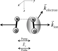
Figure 27: Molecular frame axis convention for the $C_{2v}$ NO dimer. The y-axis is along the N–N bond. Both pump and probe laser polarizations are parallel to the y-axis.

The pump transition dipole is directed along the MF $y$-axis – the N–N bond axis. The pump transition therefore forms an anisotropic distribution of excited (NO)${}_{2}^{\ast}$ states in the LF with the N–N bond aligned along the pump laser polarization axis. As we are concerned with intermediate configurations in (NO)${}_{2}^{\ast}$ evolution, we consider therefore the photoionization probing of (NO)${}_{2}^{\ast}$ , which leads predominately to dissociative ionization as shown in Fig. 26. The dissociative ionization of (NO)${}_{2}^{\ast}$ produces NO⁺ fragments strongly directed along the laser polarization axis. The NO⁺ fragment recoil direction therefore indicates the lab frame direction of the N–N bond (MF $y$-axis) prior to ionization. Rotating the electron momentum vector into the fragment recoil frame (RF) on an event-by-event basis allows for reconstruction of the (NO)${}_{2}^{\ast}$ photoelectron angular distribution in the RF, rather than the LF. Here the RF coincides with the MF, differing only by azimuthal averaging about the N–N bond direction. Out of all fragment recoil events, only those directed (“up” or “down”) along the parallel pump and probe laser polarization axis were selected. Importantly, by choosing events from this selected set, the data is restricted to excited state ionization events arising from interactions with the MF $y$-component of the ionization transition dipole only. As discussed below, this restriction greatly limits the allowed partial waves for the emitted electron, especially in the present case where only a single cation electronic continuum is accessed [Gessner2006].

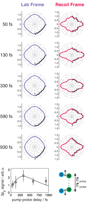
Figure 28: Coincidence-Imaging Spectroscopy of (NO)₂ photodissociation at 210nm showing LF (left) and RF (right) photoelectron angular distributions (PADs) from the 9.9-10.3 eV dissociative ionization region of Fig. 26. The laser polarizations and RF axes are along the y-direction, as shown (bottom right). The LF PADs show featureless and almost invariant behaviour. The RF PADs show strong anisotropies which vary with time. The fit curves (solid lines) include even order Legendre polynomials $P_{L}(\cos\theta)$ up to $L=4$ for the LF and up to $L=8$ for the RF. The average partial wave contribution expected from Rydberg 3p_y ionization is plotted as a function of time (bottom left). The time dependence of the intermediate configuration extracted from the TRPES data of Fig. 26 and is plotted here as the solid line, agreeing well with the time dependence of the 3p_y ionization contribution. This substantiates the intermediate configuration as being of Rydberg 3p_y character. For details see the text.

In Fig. 28 time-resolved lab and RF PADs arising from photoionization of (NO)${}_{2}^{\ast}$ in the 9.9–10.3 eV band of Fig. 26 are presented. This dissociative ionization region contains significant contributions from the intermediate (NO)${}_{2}^{\ast{\dagger}}$ configuration. In general, the time dependence of PADs relates to the evolution of excited state electronic structure, as discussed in Section TIME-RESOLVED PHOTOELECTRON SPECTROSCOPY OF NON-ADIABATIC DYNAMICS IN POLYATOMIC MOLECULES Published in Advances in Chemical Physics, Volume 139 (ed S. A. Rice), John Wiley & Sons, Inc., Hoboken, NJ, USA. doi: 10.1002/9780470259498.ch6. Here, the LF PADs have a largely isotropic character that show no discernible change with time, obscuring information about excited state dynamics. By contrast, the RF PADs show a highly anisotropic character and a variation with time delay. The solid lines in the polar plots of Fig. 28 are fits to an expansion in Legendre polynomials $P_{L}(\cos\theta)$,

$$I(\theta)=\sum_{L}\mathcal{B}_{L}P_{L}(\cos\theta).$$ (57)

For the RF PADs only even $L$ terms were non-zero with $L\leq 8$ in this fit. Increasing the maximum value of $L$ did not improve the fit to the data, and odd $L$ coefficients were found to converge to zero in the fits, in agreement with the up-down symmetry of the RF PADs.

Interestingly, the RF PADs have dominant intensity perpendicular to the laser polarization axis. An A₁ Rydberg 3s intermediate state would most likely yield maximum intensity parallel to the laser polarization axis, contrary to what is observed, since a 3s Rydberg state would ionize to primarily form p-wave ($l=1$ electrons). As can be seen from visual inspection of the data, the ratio of perpendicular to parallel photoelectron intensity varies with time, going through a maximum at around 0.3 ps before decaying again to smaller values. This “model-free” result rules out the A₁ Rydberg 3s state as the intermediate configuration. Corroborated by ab initio calculations [Levchenko2006], the RF PADs were modeled using states of B₂ symmetry. It was also assumed that the molecule largely retains $C_{2v}$ symmetry, supported by the retention of planarity during dissociation [Gessner2006, Levchenko2006] as deduced from vector correlation measurements.

To proceed further, detailed analysis of the RF PADs is required. The outgoing free electron partial waves are decomposed into symmetry-adapted spherical harmonics [Chandra1987, Underwood2000], as given by Eq. (21). For $C_{2v}$ , these harmonics are described by their $C_{2v}$ symmetry and by $l_{|\lambda|}$ , where $l$, $|\lambda|$, are the orbital angular momentum and projection quantum numbers, respectively. Values of $l=0,1,2\dots$ are labeled s, p, d$\dots$ whereas values of $|\lambda|=0,1,2\dots$ are labeled $\sigma,\pi,\delta\dots$. For the case of the NO dimer, ionization of a $B_{2}$ electronic state to an $A_{1}$ cation state via a y-polarized transition (also of $B_{2}$ symmetry) means that the free electron must have $A_{1}$ symmetry in order to satisfy the requirement in Eq. (35). This significantly restricts the allowed free electron states. Since the fit to Legendre polynomials required $L\leq 8$, partial waves with $l=0\dots 4$ are required to model the data. The $A_{1}$ symmetry partial waves with $l\leq 4$ are: s_σ, p_σ, d_σ, d_δ, f_σ, f_δ, g_σ, g_δ, and g_γ. In general the s, p, and d waves were dominant. Modelling of the data would therefore require 9 partial wave amplitudes and 8 relative phases, and so clearly a unique fit to the data was not possible. However it was possible to determine the range of partial wave amplitudes that could reproduce the shape of the RF PADs using the following method to systematically vary the model parameters. From a starting set of initial partial wave parameters (amplitudes and phases), the downhill simplex method [Nelder1965] was employed to adjust the sum of differences between the model and experimental $\mathcal{B}_{L}$ coefficients. This optimization process adjusted the parameters such that the agreement between model and experimental $B_{L}$ coefficients was better than the experimental uncertainty. This optimization process was carried out in 3 stages: (i) only s_σ, p_σ, d_σ and d_δ amplitudes and phases were optimized with all other parameters held constant (ii) s_σ, p_σ, d_σ and d_δ amplitudes and phases were held constant at the optimized values found in the previous step (iii) all parameters were optimized, starting with the values found in the two previous steps. This process was carried out for 32 different sets of starting parameters using the same set of initial parameters for the five time delays.

In order to calculate the RF PAD for a set of partial wave amplitudes and phases we use Eq. (54) to first calculate the MF PAD. The MF is defined with the $z$-axis along the $C_{2v}$ symmetry axis, the $y$-axis along the N–N bond, and the $x$-axis perpendicular to the molecular plane. The RF plane is defined with the $z$-axis along the N–N bond direction. In order to calculate the RF PAD from the MF PAD, a rotation is applied to bring the MF $z$-axis to the RF $z$-axis. The resulting PAD is then azimuthally averaged about the $z$-axis (the N–N direction),

$$I(\theta)=\int\mathrm{d}\phi\sum_{LMM^{\prime}}\beta^{\mathrm{M}}_{LM}D_{MM^{\prime}}^{L}(\pi/2,\pi/2,0)Y_{LM^{\prime}}(\theta,\phi).$$ (58)

Performing the integration over $\phi$ analytically yields

$$\mathcal{B}_{L}=2\pi\sum_{M}\beta^{\mathrm{M}}_{LM}Y^{\ast}_{LM}(\pi/2,0)$$ (59)

In order to obviate the dependence of our conclusions upon any specific partial wave amplitude, the amplitudes were contracted into two sets: those expected from 3p_y ionization and those not. Ionization of a dimer 3p_y Rydberg state via a $y$-polarized transition would, in an “atomic” $\Delta l=\pm 1$ picture of Rydberg orbital ionization, produce only electrons with $s_{\sigma}$, $d_{\sigma}$, $d_{\delta}$ character. Therefore, the ratio of [$s_{\sigma}+d_{\sigma}+d_{\delta}$] to the sum of all other contributions $\Sigma_{pfg}$ is a measure of 3p_y Rydberg character in the (NO)${}_{2}^{\ast}$ excited electronic states. In Fig. 28 (bottom) we plot the time dependence of this ratio, labelled ”3p_y signal”, showing that dimer 3p_y Rydberg character rises from early times, peaks at  330 fs and then subsequently falls. The solid curve is the time dependence of the intermediate configuration extracted from Fig. 26, showing that the 3p_y character follows the time behaviour of the intermediate (NO)${}_{2}^{\ast{\dagger}}$ configuration. The agreement substantiates (NO)${}_{2}^{\ast{\dagger}}$ as being of 3p_y character.

Ab initio studies fully support this picture [Levchenko2006]. Briefly, a very bright diabatic charge transfer (valence) state carries the transition oscillator strength. At 210nm, a vibrationally excited (roughly estimated, $\nu_{1}\sim 4$) adiabatic (NO)${}_{2}^{\ast}$ state of mixed charge-transfer/Rydberg character is populated. This quickly evolves, via N=O stretch dynamics, towards increasing 3p_y Rydberg character, forming the (NO)${}_{2}^{\ast{\dagger}}$ state. The 140 fs initial decay constant is the time scale for the initial valence state to develop intermediate 3p_y character and explains the emergence of 3p_y ionization dynamics seen in Fig. 28 at intermediate time scales ((NO)${}_{2}^{\ast{\dagger}})$. The 590 fs sequential time constant is the time scale for evolution of the dimer 3p_y configuration to free products via intramolecular vibrational energy redistribution (IVR), coupling the N=O stretch to the low frequency N–N stretch and other modes. Due to photofragment indistinguishability, the dimer 3p_y state correlates adiabatically to free NO(A, 3s) + NO(X) products without any curve crossings. With respect to the 3s Rydberg state, a dimer A₁ Rydberg 3s state was indeed found but at lower energy than the bright valence state and does not cross the latter in the FC region [Levchenko2006]. It is therefore likely that the dimer 3s state does not participate in the dissociation dynamics except perhaps far out in the exit valley where the dimer 3s and 3p states become degenerate and strongly mix.

M Photostability of the DNA Bases

The UV photostability of biomolecules is determined by the competition between ultrafast excited state electronic relaxation processes. Some of these, such as excited state reaction, photodissociation or triplet formation, can be destructive to the molecule. In order to protect against these, nature designed mechanisms which convert dangerous electronic energy to less dangerous vibrational energy. However, in order to have non-zero efficiency, any such protective mechanisms must operate on ultrafast time scales in order to dominate over competing photochemical mechanisms that potentially lead to destruction of the biomolecule. In DNA, the nucleic bases are not only the building blocks of genetic material but are also the UV chromophores of the double helix. It has been suggested that DNA must have photoprotective mechanisms which rapidly convert dangerous electronic energy into heat [Kohler2004].

The purine bases adenine and guanine and the pyrimidine bases cytosine, thymine, and uracil are all heterocycles. They typically have strong $\pi\pi^{\ast}$ UV absorption bands and, due to the lone electron pairs on the heteroatoms, have additional low-lying n$\pi^{\ast}$ transitions. Furthermore, for some bases $\pi\sigma^{\ast}$ states are also in a similarly low-energy range. This can lead to rather complex photophysical properties. Of all the bases, adenine has been most extensively studied [Kohler2004]. In the gas phase, the 9H tautomer of isolated adenine is the lowest energy and most abundant form. Two competing models were proposed to explain the photophysics of isolated adenine involving these low-lying states. One predicted internal conversion from the initially excited $\pi\pi^{\ast}$ state to the lower n$\pi^{\ast}$ state along a coordinate involving six-membered ring puckering [Broo1998]. This would be followed by further out-of plane distortion, initiating relaxation back to the S₀ ground state. An alternate model suggested that along the 9-N H-stretch coordinate a two-step relaxation pathway evolves via conical intersections of the $\pi\pi^{\ast}$ state with a repulsive $\pi\sigma^{\ast}$ state, followed by decay back to the S₀ ground state [Sobelewski2002]. Due to the repulsive character of the $\pi\sigma^{\ast}$ state, this mechanism was suggested to be highly efficient. More recently, various other possible relaxation pathways have been suggested [Perun2005, Marian2005, Blancafort2006]. The relative importance of the electronic relaxation channels in adenine has been a matter of some debate.

A time-resolved ion yield study of adenine excited state dynamics yielded an excited state lifetime of $\sim 1$ ps and seemed to support the model of internal conversion via the n$\pi^{\ast}$ state along a coordinate involving six-membered ring puckering [Kang2002]. In order to determine the global importance of the $\pi\sigma^{\ast}$ channel, a comparison of the primary photophysics of adenine with 9-methyl adenine will be useful, as the latter lacks a $\pi\sigma^{\ast}$ channel at the excitation energies of concern here. The first study of this type revealed no apparent changes in excited state lifetime upon methylation at the N9 position [Kang2003]: a lifetime of $\sim 1$ ps was observed for both adenine and 9-methyl adenine. This was interpreted as evidence that the $\pi\sigma^{\ast}$ is not involved in adenine electronic relaxation.

By contrast, the first TRPES studies compared adenine electronic relaxation dynamics at two different wavelengths, 266 nm vs. 250 nm, and concluded that the $\pi\sigma^{\ast}$ state may indeed be important [Ullrich2004, Ullrich2004a]. Additional evidence of $\pi\sigma^{\ast}$ state participation obtained from H-atom loss experiments [Hunig2004, Zierhut2004]. Hydrogen atom detection is highly sensitive and can reveal even minor H-atom loss channels. The observation of fast hydrogen atoms following UV excitation of adenine is a compelling argument for the $\pi\sigma^{\ast}$ state: fast H atoms result from an excited state potential which is repulsive in the N9H coordinate. Although this shows that a $\pi\sigma^{\ast}$ channel exists, it might play only a minor role since the H-atom quantum yield remains unknown. A more detailed time-resolved ion yield study comparing adenine with 9-methyl adenine photophysics revealed further insights [Canuel2005]. The excited state decay dynamics of adenine at 266 nm excitation required a bi-exponential fit using two time constants: a fast component decaying in 0.1 ps followed by a slower component with a 1.1 ps lifetime. Interestingly, 9-methyl adenine also exhibited that same two time constants of 0.1 ps and 1.1 ps. This again led to the suggestion that the $\pi\sigma^{\ast}$ state was not strongly involved in the dynamics, supporting the earlier ion yield experiments but contradicting the TRPES results.

Figure 29: TRPES spectra for adenine (left) and 9-methyl adenine (right), pumped at $\lambda_{\mathrm{pump}}=267$ nm and and probed at $\lambda_{\mathrm{probe}}=200$ nm. The time dependence is plotted using a linear/logarithmic scale with a linear scale in the region $-0.4$–$1.0$ ps and a logarithmic scale for delay times $1.0$–$10.0$ ps.

More recently, a new TRPES study compared adenine with 9- methyl adenine [Satzger2006], as shown in Fig. 29. The behaviour of the two molecules appears quite similar but there are important differences, as discussed below. Both molecules exhibit a broad spectral feature that covers the 7.5–10.8 eV electron binding energy (E${}_{b})$ range. This feature, peaking towards 10.8 eV, decays quickly and, beyond 500 fs, transforms into a second spectral feature spanning the 8.5–10.8 eV (E${}_{b})$ range. This second spectrum grows smoothly between 8.5–9.6 eV and is flat between 9.6–10.8 eV. This feature decays more slowly, in about 3 ps. Beyond $\sim 6$ ps, no remaining photoelectron signal was observed. Global 2D non-linear fitting algorithms determined that two exponential time constants were needed to fit these data. For 9-methyl adenine these were $\tau_{1}=70\pm 25$ fs and $\tau_{2}=1.1\pm 0.1$ ps. For adenine, these were $\tau_{1}=40\pm 20$ fs and $\tau_{2}=1.2\pm 0.2$ ps. Note that the two time constants for these molecules are the same within errors and agree quantitatively with the two time constants previously reported in the ion yield experiments [Canuel2005].

Figure 30: Decay associated spectra for adenine (dashed lines) and 9-methyl adenine (solid lines), extracted from the 2D TRPES spectra using global fitting procedures. Both molecules were fit by the same two time constants: $\tau_{1}\leq 0.1$ ps and $\tau_{2}\sim 1.1$ ps, agreeing quantitatively with previous results. The spectra, however, are very different for adenine as compared to 9-methyl adenine. For details, see the text.

Although the time constants for adenine and 9-methyl adenine are very similar, the associated photoelectron spectra reveal important differences that are obscured in ion-yield measurements. The decay associated spectra obtained from the fitting algorithm are shown in Fig. 30. The spectra of the fast ($<0.1$ ps) components are shown for adenine (dashed green) and 9-methyl adenine (solid blue). Likewise, the spectra of the 1.1 ps components for adenine (dashed red) and 9-methyl adenine (solid black) are given. The electronic states of the cations are D${}_{0}(\pi^{-1})$, D₁(n${}^{-1})$ and D₂ ($\pi^{-1})$. The expected Koopmans’ correlations would therefore be: $\pi\pi^{\ast}\rightarrow$D${}_{0}(\pi^{-1})$, D${}_{2}(\pi^{-1})$ and n$\pi^{\ast}\rightarrow$D${}_{1}($n${}^{-1})$. As detailed elsewhere [Satzger2006], the spectra of the 1.1 ps component correspond to the n$\pi^{*}\rightarrow$D₁(n${}^{-1})$+e^- ionizing transitions. Although the form of the n$\pi^{\ast}$ spectra are similar, the yield (amplitude) of n$\pi^{\ast}$ state is considerably reduced in adenine as compare to 9-methyl adenine. The most significant difference lies in the form of the spectra of the short-lived 0.1 ps component: the spectrum of 9-methyl adenine (blue solid) appears as two lobes with a gap in between whereas the spectrum of adenine (dashed green) appears as a broad spectrum without a gap.

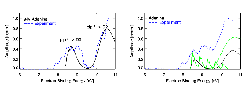
Figure 31: Decay associated spectra of the short-lived state compared with calculated FC spectra for 9-methyl adenine (right) and adenine (left). In 9-methyl adenine, the $\pi\pi^{\ast}\rightarrow$D${}_{0}(\pi^{-1})$, D${}_{2}(\pi^{-1})$ transitions leave a FC gap. In adenine, this gap is filled by the $\pi\sigma^{*}$ ionizing transitions.

In Fig. 31, we compare the associated spectrum of the fast component in 9-methyl adenine with calculated [Satzger2006] Franck-Condon (FC) structures for the $\pi\pi^{*}\rightarrow$D${}_{0}(\pi^{-1})$+e^- (solid line) and $\pi\pi^{*}\rightarrow$D${}_{2}(\pi^{-1})$+e^- (dash-dotted line) ionizing transitions. The two separated peaks agree well with the FC calculations, strongly suggesting that the short-lived state in 9-methyl adenine is the $\pi\pi^{\ast}$ state. By contrast, adenine contains an additional contribution which fills in the gap between the $\pi\pi^{*}\rightarrow$D${}_{0}(\pi^{-1})$+e^- (black solid) and $\pi\pi^{*}\rightarrow$D${}_{2}(\pi^{-1})$+e^- (black dotted) transitions. This gap is filled from the left by transitions due to $\pi\sigma^{*}\rightarrow$D${}_{0}(\pi^{-1})$+e^- (green solid) and from the right by $\pi\sigma^{*}\rightarrow$D${}_{2}(\pi^{-1})$+e^- (green dashed) ionizing transitions. These calculated FC structures provide strong evidence that the $\pi\sigma^{*}$ is present in adenine but absent in 9-methyl adenine [Satzger2006]. Adenine has two fast relaxation channels from the $\pi\pi^{*}$ state, whereas 9-methyl adenine has only one. This also explains why the yield (amplitude) of n$\pi^{\ast}$ state is reduced in adenine as compare to 9-methyl adenine. The fact that the two fast relaxation channels in adenine have very similar time constants is the reason why the ion yield experiments showed no apparent difference in lifetimes between adenine and 9-methyl adenine. Once again, the importance of measuring (dispersed) photoelectron spectra as opposed to (integrated) ion yield spectra is apparent.

Chapter Conclusion

Our goals were to elucidate important physical concepts in energy-angle resolved TRPES and to illustrate the range of its applicability to problems in molecular dynamics. We discussed general aspects of femtosecond pump-probe experiments from both the wavepacket and the frequency domain point of view. Experimentalists are, in principle, free to choose a final state through which to observe the wavepacket dynamics of interest. We emphasized the critical role of the choice of final state in determining both the experimental technique (e.g., collection of photons or particles) and the information content of an experiment (averaged or state-resolved). The molecular ionization continuum has rich structure which can act as a template onto which multi-dimensional wavepacket dynamics may be projected. The set of electronic states of the cation are sensitive to both the electronic population dynamics and the vibrational dynamics in the excited state, whereas the free electron continua are sensitive to the electronic population dynamics and the molecular frame alignment dynamics. In sum, TRPES and its variants are well suited to the study of excited state polyatomic dynamics because of their sensitivity to both electronic configurations and vibrational dynamics, the universal nature of photoionization as a probe, and the dispersed (energy- and angle-resolved) nature of the measurement.

A powerful variant, TRCIS, measures energy-resolved and 3D angle-resolved photoions and photoelectrons in coincidence, yielding unprecedented details about complex molecular photodissociations. However, TRCIS has potential beyond the ability to observe time-resolved molecular frame excited state dynamics. For example, in even more complex dissociation problems, it may be very difficult to “follow” the excited state dynamics all the way from initial excitation to final product emission. In such cases, one is tempted to resort to statistical models of the dynamics such as phase space theory. TRCIS provides a new opportunity to follow the time evolution of the product states distributions. For example, product attributes such as photofragment kinetic energy and angular distributions, photofragment angular momentum polarization and $\mu-v-J$ correlations may all now be measured as a function of time. We expect that the time evolution of these will be related to the divergence of phase space flux during dissociation and may well provide new insights into the timescales for the onset of and the extent of statisticality in energized molecules.

Future applications of TRPES and its variants will undoubtedly benefit from ongoing developments in detector technologies, femtosecond and attosecond laser sources, nonlinear optical frequency conversion schemes, and developments in free electron lasers and forth generation synchrotron light sources. TRPES research will include molecular-frame measurements, photofragment-photoelectron scalar and vector correlations, extreme time scales, and innershell dynamics. The use of shaped, intense nonresonant laser fields to create field-free alignment in polyatomic systems [Lee2006, Friedrich1995, Seideman1995, Peronne2003, Lee2004, Bisgaard2004, Berakdar2003, Dooley2003, Larsen2000, Machholm2001, Stapelfeldt2003, Sugny2004, Underwood2003, Underwood2005, Jauslin2005, Tanji2005, Sakai2003] will combine with TRPES and TRCIS to help probe molecular-frame dynamics. Further development of the multiply differential photoelectron-photofragment coincidence and coincidence-imaging methods will permit highly detailed investigation of statistical and nonstatistical photoinduced charge and energy flow, an area of fundamental dynamical interest and of interest in applications to the gas-phase photophysics of biomolecules. The development of high average power femtosecond VUV/XUV sources and the dawn of attosecond science present the possibility of probing highly excited states, core dynamics, and electron correlation in real time. Equally important are ongoing theoretical developments in ab initio molecular dynamics methods for studying non-adiabatic processes in polyatomic molecules (see, for example ref. [Martinez2006] and references therein). New methods for calculating photoionization differential cross sections (see, for example ref. [Suzuki2004] and references therein) will play an increasingly important role in the future of TRPES. These experimental and theoretical challenges will, we expect, be met by many researchers, surely leading to exciting new developments in the dynamics of polyatomic molecules.