Quantum-enhanced interferometry and the structure of twisted states

Abstract

Preparation of a non-classically correlated state is the first step of any quantum-enhanced interferometric protocol. An efficient method is the one-axis twisting, which entangles a collection of initially uncorrelated particles by means of two-body interactions. Here we investigate the limits of the quantum improvement which can be reached with this method in realistic experimental conditions. We demonstrate that the usefulness of this entangling mechanism is a result of fine structures introduced into the quantum state. The scale at which these structures vary allows us to identify the minimal requirements for the precision of the complete interferometric sequence. Our results—especially the explanation of the underlying principle of the entangling method—may help to develop ultra-precise interferometers.

Introduction—Generation of many-body entangled states for future applications in precise interferometry is a challenging task. With photons, it can be accomplished by creating a squeezed state of light which is fed into one of the interferometer’s arms knight_qo . Here squeezing refers to the reduction of the fluctuations of one of the quadratures of the electromagnetic field. The concept of squeezing can be—to some extent—transferred to the atomic domain. However, since coherences between different atom number states are forbidden ssr_wick , a single-mode squeezed state of massive particles does not exist. Nevertheless, squeezing—in this context called spin-squeezing—can be generated by reducing the fluctuations of the atom number difference between the two arms of the interferometer kitagawa1993squeezed ; wineland1994squeezed . This reduction is usually achieved using the repulsive two-body interactions between the atoms sorensen2001many .

In the pioneering work esteve2008squeezing , spin-squeezing was observed in a collection of ultra-cold rubidium atoms trapped in a double-well potential. The following experiments employed a technique called one-axis twisting (OAT) to squeeze the fluctuations between two hyper-fine states of ultra-cold atoms appel2009mesoscopic ; gross2010nonlinear ; riedel2010atom ; oat1 ; nori ; polzik . In this approach, first discussed in kitagawa1993squeezed , particles in a coherent two-mode state radcliffe1971some are dynamically entangled due to collisions. Spin-squeezing emerges immediately as the interactions start to operate. At some moment, however, spin-squeezing is lost, yet this does not mean the state is useless for precise interferometry. To contrary, the amount of useful entanglement continues to grow pezze2009entanglement , reaching the maximal attainable value greenberger1989going . This effect—loss of squeezing accompanied by the increase of the entanglement useful for interferometry witnessed by the Fisher information—has been recently observed in the experiment smerzi_ob .

Interferometry with matter-waves seems particularly promising for future realistic metrological applications schmied_rmp . This is because massive particles can strongly interact with the external field imprinting the phase, giving high interferometric signal. Moreover, two-body collisions of atoms allow for creation of many-body entangled states without the mediating element, such as a crystal used for the parametric down conversion of light pdc1 ; pdc2 .

In this work, we identify the underlying mechanism responsible for high interferometric efficiency of the OAT states. We consider two emblematic transformations—the Mach-Zehnder interferometer (MZI) and a generalized beam-splitter (BS)—both accessible with current experimental techniques appel2009mesoscopic ; gross2010nonlinear ; riedel2010atom ; smerzi_ob ; berrada2013integrated ; smerzi_twin . We show that these interferometers, combined with the measurement of the number of particles in each output port, provide an ultra-high phase sensitivity. We also discuss the influence of the detection imperfections. Those come from the limited control over the interaction strength or the duration of the OAT procedure as well as the imprecise measurement of the number of particles. Our results contribute to the understanding of the general features of the quantum nonlinear rotator rotator . They may also find application to the developing field of quantum-enhanced interferometry operating on cold-atom ensembles polzik ; non_condensed and Bose-Einstein condensates. The experimental achievement of smerzi_ob underlines the practical relevance of the entangled—but not spin-squeezed—states. The content of our work emphasizes the practical significance of even further-correlated OAT states for ultra-precise interferometry. Other authors studied the role of decoherence in the OAT procedure (see for example kolo ; ferrini ). We focus on the implementation of the OAT states and emphasize the role of the precise detection in maintaining high sensitivity.

Twisted states and quantum interferometry—Usually, an interferometer consists of two arms through which either a pulse of light- or a matter-wave moves. During this propagation, a relative phase $\theta$ is imprinted between the arms which later intersect to give an interference signal. From this output, the value of $\theta$ is deduced.

The OAT is a method of preparation of an entangled state, which is injected into an interferometer and it works as follows. Take a pure Bose-Einstein condensate in an equal superposition of modes $a$ and $b$, i.e.,

$$|\psi\rangle=\frac{1}{\sqrt{N!}}\left(\frac{\hat{a}^{\dagger}+\hat{b}^{\dagger}}{\sqrt{2}}\right)^{N}|0\rangle,$$ (1)

where $\hat{a}^{\dagger}$ and $\hat{b}^{\dagger}$ are the corresponding creation operators. The goal is to transform this separable state of $N$ particles into an entangled one. This is achieved in the absence of tunneling between the modes, when the evolution is triggered by the two-body interactions. We denote by $\chi^{-1}$ the associated timescale and have the two-mode Hamiltonian

$$\hat{H}=\hbar\chi\hat{J}_{z}^{2}.$$ (2)

Here $\hat{J}_{z}$ is one member of a triad of angular momentum operators $\hat{J}_{x}=\frac{1}{2}(\hat{a}^{\dagger}\hat{b}+\hat{b}^{\dagger}\hat{a})$, $\hat{J}_{y}=\frac{1}{2i}(\hat{a}^{\dagger}\hat{b}-\hat{b}^{\dagger}\hat{a})$, and $\hat{J}_{z}=\frac{1}{2}(\hat{a}^{\dagger}\hat{a}-\hat{b}^{\dagger}\hat{b})$. The evolution of the initial coherent state (1) with the Hamiltonian (2) gives

$$|\psi_{\alpha}\rangle=e^{-i\alpha\hat{J}_{z}^{2}}|\psi\rangle,$$ (3)

where $\alpha=\chi t$. The effect of interactions can be pictured using the mode occupation states $|m\rangle$, which denote $\frac{N}{2}+m$ particles in mode $a$ and $\frac{N}{2}-m$ in $b$ with $m\in[-\frac{N}{2},\frac{N}{2}]$. It this basis, the state (3) reads

$$|\psi_{\alpha}\rangle=\sum_{m=-\frac{N}{2}}^{\frac{N}{2}}e^{-i\alpha m^{2}}C_{m}|m\rangle,$$ (4)

with $C_{m}=\sqrt{\frac{1}{2^{N}}\binom{N}{\frac{N}{2}+m}}$. The action of the Hamiltonian (2) imprints the $\alpha$-dependent phase which is quadratic in $m$. For most values of $\alpha$, this phase jumps rapidly between the states $|m\rangle$ and $|m+1\rangle$. This is an important property of the OAT, and it is useful for the analytical calculations.

The OAT procedure transforms the coherent state (1) into the entangled one (3) and is usually considered in the relation to the spin-squeezing parameter wineland1994squeezed ; sorensen2001many

$$\xi^{2}=N\frac{\big{\langle}(\Delta\hat{J}_{n_{1}})^{2}\big{\rangle}}{\langle\hat{J}_{n_{2}}\rangle^{2}+\langle\hat{J}_{n_{3}}\rangle^{2}}.$$ (5)

Each $\hat{J}_{n_{i}}=\hat{\vec{J}}\cdot\vec{n}_{i}$ is a scalar product of the vector of angular momentum operators $\hat{\vec{J}}=[\hat{J}_{x},\hat{J}_{y},\hat{J}_{z}]$ and a unit vector $\vec{n}_{i}$ ($\vec{n}_{1}$, $\vec{n}_{2}$, and $\vec{n}_{3}$ are orthogonal), while $\Delta\hat{J}_{n_{1}}=\hat{J}_{n_{1}}-\big{\langle}\hat{J}_{n_{1}}\big{\rangle}$. When $\xi^{2}<1$, the state is called spin-squeezed, and it follows that it is particle-entangled and useful for sub shot-noise (SSN) metrology pezze2009entanglement ; giovannetti2006quantum . This is because the phase sensitivity can be linked to the spin-squeezing by the formula $\Delta\theta\propto\xi/{\sqrt{N}}$. Note that $\xi^{2}<1$ can happen only when the denominator of Eq. (5) is large. Since the angular momentum operators couple the neighbouring states $|m\rangle$ and $|m+1\rangle$, then, according to Eq. (4), their average value contains phase factors $e^{\pm 2im\alpha}$. Apart from $\alpha\simeq k\,\pi$ with $k\in\mathbb{Z}$, these phase factors quickly oscillate. As a result, the denominator of Eq. (5) is strongly suppressed. This means that within one period of evolution the state can be significantly spin-squeezed only for small $\alpha$ (i.e., short times), as observed in the experiment smerzi_ob and in agreement with the numerically calculated $\xi^{2}$, which optimized over the direction of $\vec{n}_{1}$ at each $\alpha$ is drawn in Fig. 1 with dotted green line. Analytical estimates show that indeed the OAT generates spin-squeezed states only for $\alpha\lesssim N^{-\frac{1}{2}}$ pezze2009entanglement , when the phase variations are smooth on the $m\rightarrow m+1$ increment . This means that for large $N$ the presence of spin-squeezing does not last long.

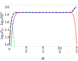
Figure 1: (color online) The QFI from Eq. (8) optimized over the direction of $\vec{n}$ (dashed black line) compared to the QFI for the BS (solid blue line) and for the MZI (solid red line). The inverse of $\xi^{2}$ calculated using Eq. (5) optimized over the direction of $\vec{n}_{1}$ is shown with a green dotted line. All quantities are drawn for $N=100$ particles.

Although $\xi^{2}>1$ at later times, the state (3) is still useful for SSN interferometry pezze2009entanglement ; smerzi_twin . To demonstrate this, note that an interferometer imprints $\theta$ through a unitary transformation

$$\hat{U}_{n}(\theta)=e^{-i\theta\hat{J}_{n}}.$$ (6)

Similarly to Eq. (5), $\hat{J}_{n}=\hat{\vec{J}}\cdot\vec{n}$ while different directions of $\vec{n}$ refer do distinct interferometric transformations. When $\vec{n}$ is oriented along the $x$ axis, thus $\hat{J}_{n}=\hat{J}_{x}$, the mode mixing transformation represents a generalized BS, while for $\hat{J}_{n}=\hat{J}_{y}$, it stands for the MZI. Finally, for $\hat{J}_{n}=\hat{J}_{z}$, the interferometer only imprints the phase $\theta$ between the modes without mixing them. Any other direction of $\vec{n}$ can be expressed as a sequence of these transformations.

If $\theta$ is estimated through a series of $\mu\gg 1$ experiments, the precision of estimation, according to the Cramer-Rao Lower Bound holevo2011probabilistic , cannot be better than

$$\Delta\theta=\frac{1}{\sqrt{\mu}}\frac{1}{\sqrt{F_{Q}}}.$$ (7)

Here, the $F_{Q}$ is the quantum Fisher information (QFI) braunstein1994statistical , which tells how much information about $\theta$ can be encoded in a state $\hat{\varrho}$ through a transformation (6). For a pure state, such as in Eq. (3), it is given by four times the variance of the generator $\hat{J}_{n}$ calculated in this state,

$$F_{Q}=4\big{\langle}(\Delta\hat{J}_{n})^{2}\big{\rangle}.$$ (8)

When $F_{Q}=N$, the lower bound for the sensitivity is the shot-noise limit (SNL) $\Delta\theta=\frac{1}{\sqrt{\mu}}\frac{1}{\sqrt{N}}$. According to Eq. (7), when the QFI is large, higher sensitivity can be reached, but $F_{Q}>N$ is only possible—allowing for SSN sensitivity—when the initial state is particle-entangled pezze2009entanglement . The QFI calculated for the state (3) is drawn with a dashed black line in Fig. 1 for each $\alpha$ maximized over the direction $\vec{n}$. It has a characteristic shape—it grows from the value of $F_{Q}=N$ for the initially uncorrelated state (1) to reach a wide plateau approximately at a moment when the spin-squeezing vanishes. Finally, through a narrow peak it strictly reaches the Heisenberg limit $F_{Q}=N^{2}$ at $\alpha=\frac{\pi}{2}$ and then symmetrically drops to $F_{Q}=N$ at $\alpha=\pi$ pezze2009entanglement . This plot shows that for the state (3), $F_{Q}\geqslant N$ for all $\alpha$.

To better understand why the QFI stays at a constant and very high level for most of the time, we focus on two types of interferometric transformations such that can be implemented in the experiment, i.e., the BS and the MZI (rotations around the $x$ and $y$ axis, respectively). When $\alpha\gtrsim N^{\frac{1}{2}}$—so that the phase in Eq. (4) quickly jumps between the neighboring states—we have

$$F_{Q} = 4\big{\langle}(\Delta\hat{J}_{x/y})^{2}\big{\rangle}\simeq 2\Big{[}\sum_{m=-\frac{N}{2}}^{\frac{N}{2}}C_{m}^{2}\beta_{m}^{2}+$$ (9a)

$$\pm \sum_{m=-\frac{N}{2}}^{\frac{N}{2}}C_{m}C_{m+2}\beta_{m}\beta_{m+1}e^{4i\alpha m}\Big{]},$$ (9b)

where $\beta_{m}=\sqrt{(N/2+m+1)(N/2-m)}$, which for large $N$ changes slowly as compared to $C_{m}$’s and can be approximated by $\frac{N}{2}$. Moreover, when $\alpha$ is not too close to $\frac{\pi}{2}$, the quickly oscillating phase “kills” the line (9b), giving $F_{Q}=\frac{1}{2}N^{2}$ both for the BS and the MZI. This happens for most values of $\alpha$, which explains the presence of the wide plateau in Fig. 1. Only when $\alpha\simeq\frac{\pi}{2}$, line (9b) starts to contribute since the phase factor is then $\sim e^{i2\pi m}=1$. For the BS, the contribution of the line (9b) is positive, so it will increase the value of the QFI up to the Heisenberg limit at $\alpha=\frac{\pi}{2}$. However, the MZI due to the opposite sign in line (9b) will experience a major drop of the QFI. These analytical estimates fully agree with the numerical results shown in Fig. 1.

Equipped with this knowledge, we show that the estimation of $\theta$ from the measurement of the population imbalance between the two output ports of either the MZI or the BS interferometer exploits the entanglement of the state (3). To this end, we calculate the related Fisher information (FI) holevo2011probabilistic given by the formula

$$F(\theta)=\sum_{m=-\frac{N}{2}}^{\frac{N}{2}}\frac{1}{p(m|\theta)}\left(\frac{\partial p(m|\theta)}{\partial\theta}\right)^{2},$$ (10)

where the probability $p(m|\theta)$ is the projection of the output state of the interferometer onto the state $|m\rangle$, i.e.,

$$p(m|\theta)=|\!\left\langle m\right|\hat{U}_{n}(\theta)|\psi_{\alpha}\rangle|^{2}.$$ (11)

The FI measures the amount of information about $\theta$ contained in the probability $p(m|\theta)$, and the corresponding CRLB, in analogy to Eq. (7), reads

$$\Delta\theta=\frac{1}{\sqrt{\mu}}\frac{1}{\sqrt{F(\theta)}}.$$ (12)

Since the QFI sets the maximal attainable sensitivity for any measurement, $F(\theta)\leqslant F_{Q}$ holds braunstein1994statistical . For both BS and MZI transformations—chosen by aligning the direction of the interferometric rotation $\vec{n}$ by either the $x$ or $y$ axis in Eq. (11) and plugging the resulting probability into the Eq. (10)—we calculate the FI as a function of $\theta$ for each $\alpha$. For instance, for the BS, the FI is

$$F(\theta) = \sum_{m=-\frac{N}{2}}^{\frac{N}{2}}\Big{(}\beta_{m}\sin(\tilde{\varphi}_{m+1}-\tilde{\varphi}_{m})\big{|}\tilde{C}_{m+1}\big{|}+$$ (13a)

$$- \beta_{m-1}\sin(\tilde{\varphi}_{m}-\tilde{\varphi}_{m-1})\big{|}\tilde{C}_{m-1}\big{|}\Big{)}^{2}.$$ (13b)

In this expression, $\tilde{C}_{m}=\left\langle m\right|\hat{U}_{x}(\theta)|\psi_{\alpha}\rangle$ and $\tilde{\varphi}_{m}$ is its phase. On the plateau, when this phase quickly jumps between the neighbouring states, the contribution to the FI resulting from the multiplication of the line (13a) by (13b) will be negligible. Moreover, the squared sine functions can be approximated by its average value $1/2$, which leads to

$$F(\theta)\simeq\sum_{m=-\frac{N}{2}}^{\frac{N}{2}}\beta_{m}^{2}\big{|}\tilde{C}_{m}\big{|}^{2}.$$ (14)

This expression closely resembles Eq. (9a) and differs only by a constant factor of two. When $\theta\simeq 0$, so that $\tilde{C}_{m}$ remains peaked around $m=0$, we can approximate $\beta_{m}^{2}\simeq N^{2}/4$ which gives

$$F\simeq\frac{N^{2}}{4}\sum_{m=-\frac{N}{2}}^{\frac{N}{2}}\big{|}\tilde{C}_{m}\big{|}^{2}=\frac{N^{2}}{4}.$$ (15)

Note that for the MZI, in Eq. (13), the sine functions are replaced with the cosine and the minus sign between lines (13a) and (13b) is replaced by a plus. This however has no impact on the above discussion giving the same value of the FI as in Eq. (15). Therefore, for both interferometers, the estimation from the population imbalance is very efficient and gives the Heisenberg scaling for a wide range of $\alpha$’s. The outcome of our analytical considerations fully agrees with the numerical calculations of the FI directly from Eq. (10).

The result (15) is obtained for the ideal case, in absence of detection imperfections. We now make a final step and analyze the influence of such limitations.

Influence of detection imperfections—We consider two sources of imperfections which might have a dominating impact on the performance of the OAT-based interferometer. The first one results from an inadequate control over the value of $\alpha$. This might be a consequence of the limited knowledge about the strength of the two-body interactions (for instance resulting from the fluctuating magnetic field fesch_jul ; dalfovo ; zwerger ; szan ) or the lack of precise control over the duration of the OAT procedure. We account for this effect by assuming that $\alpha$, rather than fixed, fluctuates with a Gaussian probability with uncertainty $\delta\alpha$. In consequence, we replace the pure state from Eq. (3) with a mixture

$$\hat{\varrho}_{\alpha}=\int\!d\tilde{\alpha}\,P(\tilde{\alpha}-\alpha)|\psi_{\tilde{\alpha}}\rangle\left\langle\psi_{\tilde{\alpha}}\right|,$$ (16)

with $P(\tilde{\alpha})\propto\exp\left[-\tilde{\alpha}^{2}/2(\delta\alpha)^{2}\right]$. The FI from Eq. (10) is now based on the probability distribution $p(m|\theta)={\rm Tr}\left[|m\rangle\left\langle m\right|\hat{U}_{n}(\theta)\hat{\varrho}_{\alpha}\hat{U}^{\dagger}_{n}(\theta)\right]$. It is reasonable to assume that $\delta\alpha\lesssim 1$, otherwise it would be not possible to resolve even the wide plateau of Fig. 1. In this limit, the result of Eq. (15) is replaced by

$$F\simeq\frac{N^{2}}{4}\times\frac{1}{\sqrt{1+2N(\delta\alpha)^{2}}}.$$ (17)

If the control over $\alpha$ is high so that $\delta\alpha\lesssim N^{-\frac{1}{2}}$, the scaling proportional to $N^{2}$ is retained. On the other hand, when $\delta\alpha\gtrsim N^{-\frac{1}{2}}$ (or even is of the order of unity), the scaling is $F\propto N^{\frac{3}{2}}$, which still is still much better than the SNL.

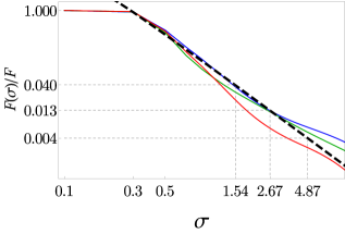
Figure 2: (color online) The FI with finite atom detection resolution $\sigma$, normalized to the FI with perfect accuracy. Three different solid lines correspond to different values of $\theta\simeq 0$ (i.e., $\theta=0.02\pi$, 0.07$\pi$ and $0.14\pi$). The dashed black line is the best fit giving a function $0.095\sigma^{-2}$. The horizontal dashed grey lines indicate the SNL for $N=100$, 300 and 1000.

Another factor which might reduce the sensitivity is the finite resolution of the atom detection $\sigma$ obert_detect ; sheet ; bloch ; paris_han . To account for this, we replace the probability (11) with

$$\tilde{p}(m|\theta)=\sum_{m^{\prime}=-\frac{N}{2}}^{\frac{N}{2}}\!\!\!R(m-m^{\prime})\,p(m^{\prime}|\theta),$$ (18)

where we take $R(m)\propto\exp[-m^{2}/2\sigma^{2}]$ as the resolution function. The finite resolution may have a much more profound effect on the FI than the uncertainty in determination of $\alpha$. This is because on the plateau, its characteristic rapid phase variations summed even over a small increment of $m^{\prime}$ oscillate down to zero. This intuitive picture is confirmed by the numerically obtained $F(\sigma)$ calculated at the plateau for different values of $\theta$, see Fig. 2. We observe that the value of FI has a universal behavior

$$F(\sigma)\propto\frac{N^{2}}{4}\times\frac{1}{\sigma^{2}}.$$ (19)

This $\sigma$-dependent scaling function does not depend on $N$ because it is rather related to the fast variation of the phase on the $m^{\prime}\rightarrow m^{\prime}+1$ increment in Eq. (18). For given $N$, this expression allows for a simple estimate of a minimal required resolution to beat the SNL. In general, $\sigma\lesssim\sqrt{N}$ is necessary to retain the SSN sensitivity, see the horizontal dashed lines in Fig. 2.

The above result is an example of a more general feature of entangled states. From the metrological point of view, such states are highly susceptible to the parameter-imprinting transformations wasak2015interferometry . This property is witnessed by the fidelity between two neighboring probabilities $p(m|\theta)$ and $p(m|\theta+\delta\theta)$ smerzi_ob . Generally speaking, probabilities which have fine structures are more prone to changes when $\theta$ is varied. In our case, those fine structures can be found in the rapid variations of the phase, which are governed by the value of $\alpha$. It is now clear that on the plateau, when $\alpha$ is high, so that the phase changes abruptly, a sophisticated detection technique is required to grasp the quantumness of the state $|\psi_{\alpha}\rangle$.

Conclusions—We have shown that the rapid phase variations of the one-axis-twisted state is the underlying mechanism responsible for its high interferometric efficiency. We have focused on two experimentally accessible transformations. The measurement of the population imbalance between the output ports provides a high sensitivity, which might be altered by the experimental imperfections. The lack of knowledge about the precise value of $\alpha$ is not as severe, as compared to the inaccurate atom number detection. The presented discussion, in particular the explanation of the essential principle of the one-axis-twisting method, might find application in other areas of ultra-precise metrology.

- (1) C. Gerry and P. Knight, Introductory Quantum Optics (Cambridge University Press, 2004)
- (2) G. C. Wick, A. S. Wightman, and E. P. Wigner, Phys. Rev. 88, 101 (1952)
- (3) M. Kitagawa and M. Ueda, Phys. Rev. A 47, 5138 (1993)
- (4) D. Wineland, J. Bollinger, W. Itano, and D. Heinzen, Phys. Rev. A 50, 67 (1994)
- (5) A. Sørensen, L.-M. Duan, J. Cirac, and P. Zoller, Nature 409, 63 (2001)
- (6) J. Esteve, C. Gross, A. Weller, S. Giovanazzi, and M. Oberthaler, Nature 455, 1216 (2008)
- (7) J. Appel, P. J. Windpassinger, D. Oblak, U. B. Hoff, N. Kjærgaard, and E. S. Polzik, Proc. Natl. Acad. Sci. USA 106, 10960 (2009)
- (8) C. Gross, T. Zibold, E. Nicklas, J. Esteve, and M. K. Oberthaler, Nature 464, 1165 (2010)
- (9) M. F. Riedel, P. Böhi, Y. Li, T. W. Hänsch, A. Sinatra, and P. Treutlein, Nature 464, 1170 (2010)
- (10) M. Takeuchi, S. Ichihara, T. Takano, M. Kumakura, T. Yabuzaki, and Y. Takahashi, Phys. Rev. Lett. 94, 023003 (2005)
- (11) J. Ma, X. Wang, C. Sun, and F. Nori, Physics Reports 509, 89 (2011), ISSN 0370-1573
- (12) T. Fernholz, H. Krauter, K. Jensen, J. F. Sherson, A. S. Sørensen, and E. S. Polzik, Phys. Rev. Lett. 101, 073601 (2008)
- (13) J. Radcliffe, Journal of Physics A: General Physics 4, 313 (1971)
- (14) L. Pezzé and A. Smerzi, Phys. Rev. Lett. 102, 100401 (2009)
- (15) D. M. Greenberger, M. A. Horne, and A. Zeilinger, Going beyond Bell’s theorem (Springer, 1989) pp. 69–72
- (16) H. Strobel, W. Muessel, D. Linnemann, T. Zibold, D. B. Hume, L. Pezzé, A. Smerzi, and M. K. Oberthaler, Science 345, 424 (2014)
- (17) A. D. Cronin, J. Schmiedmayer, and D. E. Pritchard, Rev. Mod. Phys. 81, 1051 (2009)
- (18) D. C. Burnham and D. L. Weinberg, Phys. Rev. Lett. 25, 84 (1970)
- (19) P. G. Kwiat, K. Mattle, H. Weinfurter, A. Zeilinger, A. V. Sergienko, and Y. Shih, Phys. Rev. Lett. 75, 4337 (1995)
- (20) T. Berrada, S. van Frank, R. Bücker, T. Schumm, J.-F. Schaff, and J. Schmiedmayer, Nat. Commun. 4 (2013)
- (21) B. Lücke, M. Scherer, J. Kruse, L. Pezzé, F. Deuretzbacher, P. Hyllus, O. Topic, J. Peise, W. Ertmer, J. Arlt, L. Santos, A. Smerzi, and C. Klempt, Science 334, 773 (2011)
- (22) B. C. Sanders, Phys. Rev. A 40, 2417 (1989)
- (23) T. Takano, M. Fuyama, R. Namiki, and Y. Takahashi, Phys. Rev. Lett. 102, 033601 (2009)
- (24) J. B. Brask, R. Chaves, and J. Kołodyński, arXiv:1411.0716
- (25) K. Pawłowski, D. Spehner, A. Minguzzi, and G. Ferrini, Phys. Rev. A 88, 013606 (2013)
- (26) V. Giovannetti, S. Lloyd, and L. Maccone, Phys. Rev. Lett. 96, 010401 (2006)
- (27) Indeed, the variation of the phase can be estimated by its derivative . For the initial coherent state, the maximal , giving
- (28) A. Holevo, Probabilistic and Statistical Aspects of Quantum Theory (Publications of Scuola Normale Superiore, 2011)
- (29) S. L. Braunstein and C. M. Caves, Phys. Rev. Lett. 72, 3439 (1994)
- (30) We have used the fact that the ’s and the imprinted phase are symmetric with respect to .
- (31) C. Chin, R. Grimm, P. Julienne, and E. Tiesinga, Rev. Mod. Phys. 82, 1225 (2010)
- (32) F. Dalfovo, S. Giorgini, L. P. Pitaevskii, and S. Stringari, Rev. Mod. Phys. 71, 463 (1999)
- (33) I. Bloch, J. Dalibard, and W. Zwerger, Rev. Mod. Phys. 80, 885 (2008)
- (34) P. Szańkowski, M. Trippenbach, and J. Chwedeńczuk, Phys. Rev. A 90, 063619 (2014)
- (35) D. B. Hume, I. Stroescu, M. Joos, W. Muessel, H. Strobel, and M. K. Oberthaler, Phys. Rev. Lett. 111, 253001 (2013)
- (36) R. Bücker, A. Perrin, S. Manz, T. Betz, C. Koller, T. Plisson, J. Rottmann, T. Schumm, and J. Schmiedmayer, New J. Phys. 11, 103039 (2009)
- (37) J. F. Sherson, C. Weitenberg, M. Endres, M. Cheneau, I. Bloch, and S. Kuhr, Nature 467, 68 (2010)
- (38) M. Schellekens, R. Hoppeler, A. Perrin, J. V. Gomes, D. Boiron, A. Aspect, and C. I. Westbrook, Science 310, 648 (2005)
- (39) T. Wasak, P. Szańkowski, and J. Chwedeńczuk, Phys. Rev. A 91, 043619 (2015)
- (40) The fidelity between two probability distributions and is defined as .