Semiclassical analysis of intraband collective excitations in a two-dimensional electron gas with Dirac spectrum

Abstract

Solving the initial value problem for semiclassical equations that describe two-dimensional electrons with the Dirac spectrum we found that collective excitations of the electrons are composed by a few distinct components of the oscillations. There always exist sustained plasma oscillations with well known plasmon frequency $\omega_{pl}(k)$. Additionally there are oscillations with the ’carrier frequency’ $\omega=v_{F}k$ slowly decaying in time according to a power law ($v_{F}$ and $k$ are the Fermi velocity and wavevector). The reason for onset of these oscillations has a fundamental character related to branching of the polarization function of the Dirac electrons. A strongly anisotropic initial disturbance of the electron distribution generates additional component of undamped oscillations in the form of an electron unidirectional beam which are van Kampen’s modes in the Dirac plasma.

Polarization properties of electrons determine their response to an external electrical signal, define collective plasmon and plasmon-phonon modes, as well as many other phenomena involving interaction of the charges. A fundamental and applied aspects of collective excitations in graphene-like systems were discussed in detail in several reviews Castro-rev ; SarmaReview ; NovoselovReview ; PlasmonReview ; BasovReview ; PlasmonReview1 ; PlasmonReview2 ; PlasmonReviewTHz . The polarizability of two-dimensional (2D) electrons with the linear Dirac spectrum, $\textstyle{\epsilon({p})=v_{F}p}$, differs considerably from that of the electrons with a parabolic spectrum ($\textstyle{\epsilon(p)\propto p^{2}}$) characteristic for conventional low-dimensional heterostructures. Particularly, the absence of the spectrum curvature leads to less effective screening of the Coulomb potential Castro-rev , gives rise to the divergence of the irreducible polarizability Wunsch ; Sarma ; Ryzhii_gate $\Pi(\omega,k)\propto 1/\sqrt{\omega^{2}-v_{F}^{2}k^{2}}$ at $\textstyle{\omega\rightarrow\pm v_{F}k}$ with $\omega$ and ${\bf k}$ are frequency and the 2D wavevector, respectively, $v_{F}$ is the Fermi velocity. Then, the square-root behavior of the polarizability means that $\Pi(\omega,k)$ is a double-valued function on the complex $\omega$-plane. For calculation of real characteristics of the physical system, properties of the polarizability as an analytical function on the complex $\omega$-plane is critically important. The semiclassical approach based on the analysis of the Boltzmann-Vlasov system of equations allows one to construct the principal branch of the polarizability function $\Pi(\omega,k)$ and obtain transparent and easy interpreted results. These results complement those calculated with the use of different quantum mechanical approaches in the long-wavelength limit Wunsch ; Sarma .

Recently, new nanoscope techniques were proposed to launch the excitations by a sharp tip of atom force microscope and to monitor them by the scattering type near-field optical microscope NS-1 ; NS-2 . The techniques have enabled the experimental exploration of spatio-temporal Fei-1 ; Chen-1 ; Fei-2 ; Fei-3 and time-resolved Fei-4 dynamics of the collective excitations in the graphene and graphene-like systems. Importantly, both the excitation amplitude and phase can be measured PRL-phase . Similar studies have been performed by the use of the resonant antenna plasmon launcher and near-field optical microscope Alonso . Another promising method for plasmon investigation is time-resolved electrical measurements Japan-1 ; Japan-2 . Observed in these works macroscopic effects - long-wavelength charge modes and local electric fields - can be described by using the semiclassical approach.

In this Communication, we present the semiclassical analysis of longitudinal intraband excitations of 2D electron gas with the Dirac spectrum. It is appropriate to note, that the transverse electric mode in graphene-like systems was analyzed in paper Mikhailov . We assume the $n$-doped system and restrict ourselves to excitations with $\omega$ and ${\bf k}$ for which interband processes can be neglected at a given electron concentration, $n$, and ambient temperature, $T$. Such approach is valid for $\textstyle{\hbar\omega<\epsilon(p_{F}),\,\hbar k<p_{F}}$ at $\textstyle{k_{B}T\ll\epsilon(p_{F})}$, with $p_{F}$ being the Fermi momentum and $k_{B}$ is the Boltzmann constant (detail discussion see, for example, in Ref. Castro-rev, ).

The Boltzmann-Vlasov system of equations consists of the collisionless transport equation

$$\frac{\partial F}{\partial t}+v_{F}\frac{\bf p}{p}\left.\frac{\partial F}{\partial{\bf r}}+e\frac{\partial\Phi}{\partial\mathbf{r}}\right|_{z=0}\frac{\partial F}{\partial{\bf p}}=0,$$ (1)

and the Poisson equation

$$\Delta\Phi=\frac{4\pi e\delta[z]}{\kappa}\int\frac{g\,d^{2}p}{(2\pi\hbar)^{2}}[F({\bf r,p},t)-F_{0}({\bf p})]\,.$$ (2)

Here the Dirac spectrum is assumed for the electrons confined to the sheet at $\textstyle{z=0}$. The electron coordinate and momentum $\bf r,\,p$ are the 2D vectors in the $x-y$ plane. $F({\bf r,p},t)$ is the electron distribution function, $F_{0}({\bf p})$ is that under equilibrium. $\Phi({\bf r},z,t)$ is the self-consistent electrostatic potential. In Eq. (2), $e$ is the elementary charge, $\delta[z]$ is the Dirac delta-function, $g$ is the degeneracy factor of the electron band (for graphene $g=4$). The parameter $\kappa$ depends on dielectric environment. If the electron sheet is between two materials with the dielectric constants $\kappa_{l},\,\kappa_{h}$, in final formulae one shall use $\textstyle{\kappa=(\kappa_{l}+\kappa_{h})/2}$.

For the collisionless limit it is necessary $\textstyle{\omega\tau\gg 1}$, $\textstyle{v_{F}k\tau\gg 1}$, with $\tau$ being a characteristic scattering time. For our purposes the equation (1) shall be linearized. We denote variation of the distribution function as ${\cal F}({\bf r},{\bf p},t)\equiv F({\bf r},{\bf p},t)-F_{0}({\bf p})$ and set ${\cal F}({\bf r},{\bf p},t)={\cal F}_{\bf k}({\bf p},t)\,exp(i{\bf kr})$, and ${\Phi}({\bf r},z,t)={\Phi}_{\bf k}(z,t)\,exp(i{\bf kr})$. Now Eqs. (1), and (2) take the form:

$$\frac{\partial{\cal F}_{\bf k}}{\partial t}+iv_{F}\frac{\bf kp}{p}{\cal F}_{\bf k}=-ie{\bf k}{\Phi}_{\bf k}(0,t)\frac{\partial F_{0}}{\partial{\bf p}}\,,$$ (3)

$$\frac{d^{2}{\Phi}_{\bf k}}{dz^{2}}-k^{2}\Phi_{\bf k}=\frac{4\pi e\delta[z]}{\kappa}\int\frac{g\,d^{2}p}{(2\pi\hbar)^{2}}{\cal F}_{\bf k}({\bf p},t)\,.$$ (4)

Following the Landau approach Landau-1 , we consider the initial value problem by using the Laplace transform:

$$f_{\omega,\bf k}({\bf p})\!=\!\!\!\int\limits^{\infty}_{0}\!\!{\cal F}_{\bf k}({\bf p},t)\,e^{i\omega t}dt,\,\,{\cal F}_{\bf k}({\bf p},t)\!\!\!=\!\!\!\int\limits^{\infty+i\sigma}_{-\infty+i\sigma}\!\!\!\!\!\!\!f_{\omega,\bf k}({\bf p})\,e^{-i\omega t}\,\frac{d\omega}{2\pi}\,,$$ (5)

where $\sigma>0$. Similarly, we define the transformation of the potential, $\phi_{\omega,\bf k}(z)$. Now one can easily find the solution for $f_{\omega,\bf k}({\bf p})$:

$$f_{\omega,\bf k}({\bf p})=i\frac{{\delta\cal F}_{\bf k}({\bf p})-ie\phi_{\omega,\bf k}(0){\bf k}\,dF_{0}({\bf p})/d{\bf p}}{\omega-v_{F}({\bf kp})/p}\,,$$ (6)

with $\delta{\cal F}_{\bf k}({\bf p})$ being a given initial perturbation of the electron distribution. The solution to Eq. (4), which decaying at $z\rightarrow\pm\infty$, also can be easily found. The potential at $z=0$ is:

$$\phi_{\omega,\bf k}(0)\!=\!\frac{-2\pi ie}{\kappa\,k\,\Delta(\omega,k)}\!\!\int\!\!\frac{g\,d^{2}p}{(2\pi\hbar)^{2}}\!\frac{\delta{\cal F}_{\bf k}({\bf p})}{\left[\omega-v_{F}({\bf kp})/p\right]}\!\!\equiv\!\!\frac{N(\omega,{\bf k})}{\Delta(\omega,k)}\,,$$ (7)

with $\Delta(\omega,k)=1-2\pi e^{2}\,\Pi(\omega,k)/{\kappa\,k}$ and

$$\Pi(\omega,k)\ \equiv-\int\!\!\!\frac{g\,d^{2}p}{(2\pi\hbar)^{2}}\frac{({\bf kp})/p}{\left[\omega-v_{F}({\bf kp})/p\right]}\frac{dF_{0}(p)}{dp}\,.$$ (8)

It is clear that $\Pi(\omega,k)$ has the meaning of the polarizability obtained in the semiclassical limit. $F_{0}({\mathbf{p}})$ is the Fermi distribution, then

$$\Pi(\omega,k)=\frac{\kappa\,K}{2\pi e^{2}}\left[\frac{1}{2\pi}\int^{2\pi}_{0}d\alpha\frac{\omega}{\omega-v_{F}k\cos{\alpha}}-1\right]\,,$$ (9)

$$K=\frac{e^{2}gk_{B}T}{\kappa\hbar^{2}v_{F}^{2}}\ln{\!\left[\exp{\!\left[\frac{E_{F}}{k_{B}T}+1\right]}\right]}\,,$$ (10)

where $E_{F}$ is the chemical potential.

According to the definition of the Laplace transform (5), in foregoing Eqs. (6)-(9) $\omega=\omega^{\prime}+i\omega^{\prime\prime}$ is the complex variable belonging to the upper half-plane, $\omega^{\prime\prime}>0$. Under the latter condition, the integral in Eq. (9) can be calculated as

$$\Pi(\omega,k)=\frac{\kappa\,K}{2\pi e^{2}}\left(\frac{\omega}{\sqrt{\omega^{2}-v^{2}_{F}k^{2}}}-1\right)\,.$$ (11)

The function (11) is double-valued with two branch points, $\omega=\pm v_{F}k$, as discussed in introduction.

Consider an analytical continuation of $\Pi(\omega,k)$ given by (9) to the lower half of the $\omega$-plane. We start with the use of (11) valid for all complex $\omega$-plane except the segment at the real axis $-v_{F}k\leq\omega^{\prime}\leq v_{F}k$. By choosing the cut along this segment, we select the principle branch of the function (11). Defined by such a way, $\Pi(\omega,k)$ is continuous when crossing the real axis at $|\omega|>v_{F}k$, while it undergoes a jump in its value at the cut.

As a result of this procedure, we obtain also the function $\Delta(\omega,k)$ as well-defined function in the complex $\omega$-plane. It is easy to see that this function has simple zeros on the real axis

$$\omega^{\prime}=\pm\omega_{pl}\,,\,\,\,\omega_{pl}(k)=\frac{v_{F}k\left(1+{k/K}\right)}{\sqrt{\left(1+{k/K}\right)^{2}-1}}\,,$$ (12)

which are the exact solutions of the equation $\textstyle{\Delta(\omega,k)=0}$. For what follows, it is important that $\omega_{pl}(k)>v_{F}k$.

Before to proceed with the farther analysis, let us estimate the value $K$ for the graphene. Assuming the graphene sheet over a $SiC$-substrate ($\kappa_{l}\approx 9.7,\,\kappa_{h}=1$), setting the electron concentration $n=2\times 10^{12}cm^{-2}$ and temperature $\textstyle{T=300}$ K, we obtain $E_{F}\approx 0.16\,eV$, $\textstyle{E_{F}/k_{B}T\approx 6.12}$, $p_{F}/\hbar\equiv k_{F}\approx 2.5\times 10^{6}\,cm^{-1}$, and $\textstyle{K\approx 3.9\times 10^{6}\,cm^{-1}}$. That is $k_{F}<K$ and for the semiclassical analysis we should use $\textstyle{k<k_{F}<K}$. For example, at $\textstyle{k=0.05\,K}$ we obtain $\textstyle{\omega_{pl}\approx 6.4\times 10^{13}\,s^{-1}}$ and $\textstyle{v_{F}k\approx 2\times 10^{13}\,s^{-1}}$. We refer to this set of parameters as $\kappa$-environment-I. To estimate the criteria of validity of the collisionless approximation, one needs to know the characteristic scattering time, $\tau$. The ’intrinsic’ electron-electron scattering time is of the order of $10^{-11}\,s$ Principi . Optical phonon scattering can be neglected for the above accepted parameters. Acoustical phonon scattering time at $T\leq 300\,K$ is estimated to be less than $2\times 10^{-11}\,s$ SarmaReview . Elastic scattering by imperfections is dominant. It can be determined via the phenomenological relationship for the transport time: $\tau\approx\mu E_{F}/ev_{F}^{2}$ with $\mu$ being the mobility. Assuming $\mu=2.5\times 10^{4}\,cm^{2}/V\,s$, we obtain $\tau\approx 4\times 10^{-13}\,s$ and find that the semiclassical approximation criteria are met: $\omega_{pl}\tau\approx 26\gg 1$, $v_{F}k\tau\approx 8\gg 1$.

For the graphene sheet in a high-$\kappa$ environment (for example, graphene in a solvent Ferro ), the value $K$ can be sufficiently less than $k_{F}$. Then the case $\textstyle{k\geq K}$ may be actual. For example, at $\textstyle{\kappa_{l}\approx 9.7}$, $\textstyle{\kappa_{h}=50}$, and $k=K$ ($\kappa$-environment-II) for the same electron concentration, we obtain $K\approx 7\times 10^{5}\,cm^{-1}$ and $\omega_{pl}\approx 8\times 10^{13}\,s^{-1},\,v_{F}k\approx 7\times 10^{13}\,s^{-1}$ (note, the accepted $k$ is greater than for the $\kappa$-environment-I). These estimates show that the excitations considered are rather of the THz diapason.

Now, one can perform the inverse Laplace transform to find desirable functions in the time-domain. Below, we will concentrate on the potential at $z=0$:

$$\Phi_{\bf k}(t)\equiv\Phi_{\bf k}(0,t)=\int\limits^{\infty+i\sigma}_{-\infty+i\sigma}\!\!\!\!\!\!\phi_{\omega,\bf k}(0)\,e^{-i\omega t}\,\frac{d\omega}{2\pi}.$$ (13)

According to Eq. (7), one can present $\phi_{\omega,{\bf k}}(0)$ as a fraction, where the nominator, $N(\omega,{\bf k})$, is determined by the initial perturbation, $\delta{\cal F}_{\bf k}({\bf p})$. First, we will use the typical assumption Landau-1 that the initial perturbation is such that $N(\omega,{\bf k})$ has no poles in the $\omega$-plane. Then, the analytical properties of both $\Delta(\omega,k)$ and whole integrand in (13) allow one to deform the integration contour and calculate explicitly contributions of the residues related to the zeros of $\Delta(\omega,{\bf k})$ and branch points:

$$\Phi_{\bf k}(t)=\Phi^{R}_{\bf k}(t)+\Phi^{\cal C}_{\bf k}(t)\,,$$ (14)

$$\Phi^{R}_{\bf k}(t)=-i\frac{\left[\omega_{pl}^{2}-v_{F}^{2}k^{2}\right]^{3/2}}{v_{F}^{2}kK}\times$$

$$\!\!\!\!\!\left[\phantom{\frac{A}{B}}\right.\!\!\!\!\!\!\!N(\omega_{pl},{\bf k})\exp{[-i\omega_{pl}\,t]}-N(-\omega_{pl},{\bf k})\exp{[i\omega_{pl}\,t]}\left.\phantom{\frac{A}{B}}\!\!\!\!\!\!\!\right],$$ (15)

$$\Phi^{\cal C}_{\bf k}(t)=\oint_{\cal C}\phi_{\omega,\bf k}(0)\,e^{-i\omega t}\,\frac{d\omega}{2\pi}\,.$$ (16)

In the integral (16), contour $\cal C$ encloses the cut, as shown in the inset of Fig. 1(a).

In Eq. (14), the first term oscillating with time describes the undamped plasmons excited by the initial perturbation of the distribution function. The latter specifies only the magnitude of the plasmon excitations, while their frequencies do not depend on the initial perturbation. They are determined by the zeros of $\Delta(\omega,k)$ given by Eq. (12). For $k\ll K$, one obtains ’the square root law’ Wunsch ; Sarma , $\omega_{pl}\approx v_{F}\sqrt{kK/2}$; in the opposite limit, $\omega_{pl}\rightarrow v_{F}k$.

The last term in Eq. (14) arises due to the existence of branch points in $\Delta(\omega,k)$. For electron systems with regular quadratic energy dispersion, there is no branching and such contribution does not exist. The time dependence of this term is defined by the initial perturbation. Let us consider a few examples of different initial perturbations.

First, assume that the initial perturbation is isotropic, $\delta{\cal F}_{\bf k}({\bf p})=\delta{\cal F}_{k}(p)$, i.e., for perturbed electron gas the average momentum and velocity are zero. Then,

$$N(\omega,{k})=\frac{i\Phi_{k}^{0}}{\sqrt{\omega^{2}-v_{F}^{2}k^{2}}}\,,\,\,\Phi_{k}^{0}=\!-\frac{eg}{\kappa\hbar^{2}k}\!\int\limits^{\infty}_{0}\!\!pdp\,\delta{\cal F}_{k}(p)\,,$$ (17)

where the square root should be defined as principal branch on the $\omega$-plane with the above discussed cut. Now, the contribution of the residues to the potential equals

$$\frac{\Phi^{R}_{k}(t)}{\Phi_{k}^{0}}=\frac{2\left[\omega_{pl}^{2}(k)-v_{F}^{2}k^{2}\right]}{v_{F}^{2}kK}\,cos[\omega_{pl}(k)\,t]\,.$$ (18)

The contour integral of Eq. (16) can be easily estimated for two limiting cases:

$${\frac{\Phi^{\cal C}_{k}(t)}{\Phi_{k}^{0}}\approx}\begin{cases}\displaystyle{\frac{k}{K}J_{1}(v_{F}kt)/v_{F}kt,k\ll K,}\\ \displaystyle{J_{0}(v_{F}kt),\phantom{empty!!!!}k\gg k\,,}\end{cases}$$ (19)

where $J_{0}(x),\,J_{1}(x)$ are the Bessel functions. At $t\gg 1/(v_{F}k)$, both expressions can be further simplified

$${\!\!\!\!\frac{\Phi^{\cal C}_{k}(t)}{\Phi_{k}^{0}}\approx\!\sqrt{\frac{2}{\pi}}\!}\begin{cases}\displaystyle{\frac{k}{K}\frac{\cos[v_{F}kt-3\pi/4]}{(v_{F}kt)^{3/2}},\,\,\,\,}&k\ll K\,,\\ \displaystyle{\,\,\frac{\cos[v_{F}kt\!-\!\pi/4]}{(v_{F}kt)^{1/2}},}&k\gg K\,.\end{cases}$$ (20)

Thus, the initial isotropic perturbation of the electron distribution generates two different components of electrostatic potential oscillating in time and space. The first component is, obviously, sustained regular plasmon oscillations, excited by the initial perturbation. The second component corresponds to oscillations with the ’carrier’ frequency $\omega=v_{F}k$. The oscillations decay in time according to a power law. Mathematically, they arise due to the existence of the branch points of polarization function (9). Recovering the space-dependent factor $exp[i{\bf kr}]$, one can see that $\Phi_{\bf k}^{R}$ and $\Phi_{\bf k}^{\cal C}$ components correspond to standing waves. The main panels of Figs. 1(a) and (b) show the normalized potential $\varphi_{k}^{\cal C}(t)=\Phi_{k}^{\cal C}/\Phi_{k}^{0}$ of these oscillations for two $\textstyle{\kappa}$-environments discussed above.

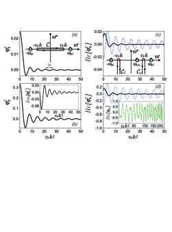
Figure 1: (color online). Normalized potential $\varphi_{\bf k}^{\cal C}(t)$ for: (a), (c) – $\kappa$-environment-I and (b), (d) – $\kappa$-environment-II; (a), (b) – isotropic initial perturbation; (c), (d) – strongly anisotropic initial perturbation, solid line - $\alpha_{0}=\pi/3$, dotted line - $\alpha_{0}=0$. Insets on (a), (c): cuts and integral paths on the $\omega$-plane; inset of (b): $\varphi_{\bf k}^{\cal C}(t)$ for weak anisotropic perturbation; inset of (d): example of temporal pattern for $\omega_{pl}\approx 2\omega_{vK}$.

Interestingly, the ratio of the magnitudes of the two components depends essentially on the wavevector. Indeed, for $k\ll K$, and $\textstyle{t\rightarrow 0}$ we obtain the estimate $\varphi_{k}^{\cal C}\approx k/2K\ll 1$. From Fig. 1(b) we see that at $k=K$ $\varphi_{k}^{\cal C}\approx 0.33$. In the opposite case, $k\gg K$, we obtain $\varphi_{k}^{C}\approx 1$. That is, the regular plasmon component is preferable excited by long-wavelength perturbations.

Then, consider an initial perturbation of the anisotropic form $\textstyle{\delta{\cal F}_{\bf k}({\bf p})=\delta{\cal F}_{k}(p){\bf pn}/p}$, with $\bf n$ being a unit vector of a preferential direction. We denote the angle between $\bf n$ and $\bf k$ as $\alpha_{0}$. For this case, at $t=0$ the perturbed electron gas receives additional momentum and nonzero velocity, while the electron density is unperturbed. The calculation gives

$$N(\omega,{\bf k})=i\frac{\Phi_{k}^{0}\cos\alpha_{0}}{v_{F}k}\left[\frac{\omega}{\sqrt{\omega^{2}-v_{F}^{2}k^{2}}}-1\right]\,,$$ (21)

where $\Phi_{k}^{0}$ formally is given by the second relationship of Eq. (17). Calculating the time-dependent potential $\Phi_{\bf k}(t)$ with this $N(\omega,{\bf k})$ function, one can use the analytical continuation discussed above, as well as Eqs. (14) - (16), and the integration contour shown in the inset of Fig. 1(a). The residue contribution to the potential is

$$\!\!\frac{\Phi_{\bf k}^{R}(t)}{\Phi_{k}^{0}}=\!-2i\cos\alpha_{0}\frac{[\omega_{pl}^{2}(k)-v_{F}^{2}k^{2}]^{3/2}}{v_{F}^{3}kK^{2}}\sin[\omega_{pl}(k)\,t]\,.$$ (22)

For the contour integral of Eq. (16), we present the results obtained for two limiting cases:

$$\frac{\Phi^{\cal C}_{\bf k}(t)}{\Phi_{k}^{0}}\!\approx\!i\cos\alpha_{0}\!\!\begin{cases}\displaystyle{\left(\frac{k}{K}\right)^{\!2}\left[\!\frac{J_{0}[v_{F}kt]}{v_{F}kt}\!-\!2\frac{J_{1}[v_{F}kt]}{[v_{F}kt]^{2}}\right]\!,k\ll K,}\\ \displaystyle{J_{1}(v_{F}kt),\phantom{emptyemptyempty!!!!}k\gg K.}\end{cases}$$ (23)

At $t=0$, both contributions $\Phi_{\bf k}^{R}$ and $\Phi^{\cal C}_{\bf k}$ equal zero. At $t\gg 1/v_{F}k$, we obtain:

$$\frac{\!\Phi^{\cal C}_{\bf k}(t)}{\Phi_{k}^{0}}\!\approx\!i\sqrt{\frac{2}{\pi}}\cos\alpha_{0}\!\begin{cases}\displaystyle{\left(\frac{k}{K}\right)^{\!2}\!\frac{\cos{[v_{F}kt-\pi/4]}}{(v_{F}kt)^{3/2}}\,,}\!\!&k\ll K,\\ \displaystyle{\,\,\,\,\frac{\cos{[v_{F}kt-3\pi/4]}}{(v_{F}kt)^{1/2}}\,,}&k\gg K\,.\end{cases}$$ (24)

Thus, weak anisotropic initial perturbation also produces two component oscillations with purely imaginary magnitude, $\Phi_{\bf k}^{R}$ and $\Phi_{\bf k}^{\cal C}$, with frequencies $\omega=\omega_{pl}(k)$ and $\omega=v_{F}k$, respectively. The latter are decaying in time. At small $t\approx 1/v_{F}k$, these oscillations are quite different from those discussed above, since such perturbation does not generate directly a space charge and an electrostatic potential. Both are developing with time. The normalized potential $\textstyle{\varphi_{\bf k}^{\cal C}(t)=\Phi_{\bf k}^{\cal C}/\Phi_{k}^{0}}$ of these oscillations is illustrated in the inset of Fig. 1(b). The oscillations magnitude depends on the angle $\alpha_{0}$. The magnitude reach maxima for $\alpha_{0}=0,\,\pi$. If $\alpha=\pi/2$, the perturbation does not excite the oscillations.

Finally, consider the extremely anisotropic initial perturbation: $\delta{\cal F}_{\bf k}({\bf p})=2\pi\delta{\cal F}_{k}({p})\,\delta[\alpha-\alpha_{0}]$, where $\alpha$ is the angle between ${\bf p}$ and $\bf k$, $\alpha_{0}$ determines the anisotropy direction. For the function $N(\omega,{\bf k})$ we obtain

$${N(\omega,{\bf k})=\frac{i\Phi_{k}^{0}}{\omega-v_{F}k\cos\alpha_{0}}},$$ (25)

with $\Phi_{k}^{0}$ still defined by Eq. (17). The function (25) has a pole at the $\omega^{\prime}$-axis: $\omega=\omega_{vK}({\bf k})\equiv v_{F}k\cos\alpha_{0}\,$. That implies that the accepted above way of the analytical continuation of the function $\Pi(\omega,k)$ is no longer applicable. Instead, one can use two cuts along semi-infinite lines in the lower part of the $\omega$-plane: $\omega=\pm v_{F}k+i\omega^{{}^{\prime\prime}},\,\omega^{{}^{\prime\prime}}\leq 0$, as shown in the inset of Fig. 1(c). Now $\Pi(\omega,k)$ is continuous across the real axis everywhere excluding points $\omega=\pm v_{F}k$ and undergoes jumps at the semi-infinite cuts. The time-dependent total potential (13) consists of four contributions:

$$\Phi_{\bf k}(t)=\Phi^{R}_{\bf k}(t)+\Phi^{{\cal C}_{l}}_{\bf k}(t)+\Phi^{{\cal C}_{r}}_{\bf k}(t)+\Phi^{vK}_{\bf k}(t)\,.$$ (26)

In contrast to the previous cases, every contribution has nonzero real and imaginary parts. The term $\Phi^{R}_{\bf k}(t)$ is the plasmon contribution determined by Eq. (15) with $N(\omega,{\bf k})$ given by (25),

$$\displaystyle{\frac{\Phi^{R}_{\bf k}(t)}{\Phi_{k}^{0}}=\frac{2\left[\omega_{pl}^{2}-v_{F}^{2}k^{2}\right]^{3/2}}{v_{F}^{2}kK(\omega_{pl}^{2}-v_{F}^{2}k^{2}\cos^{2}{\alpha_{0}})}\times}$$ (27)

$$\displaystyle{\times\{\omega_{pl}\cos[\omega_{pl}t]-iv_{F}k\cos{\alpha_{0}}\sin{[\omega_{pl}t]}\}.}$$

The terms $\Phi^{{\cal C}_{l}}_{\bf k}(t)$ and $\Phi^{{\cal C}_{r}}_{\bf k}(t)$, are the contour integrals around the left and right cuts, respectively (see Fig. 1(c)). Main panels of Figs. 1(c) and (d) display real parts of the total contribution $\textstyle{\Phi_{\bf k}^{\cal C}=\Phi_{\bf k}^{{\cal C}_{l}}+\Phi_{\bf k}^{{\cal C}_{r}}}$ from the contour integrals. Latter can be found explicitly in the limiting case $t\gg 1/(v_{F}\,k\,\sin^{2}{\alpha_{0}})$:

$$\!\!\frac{\Phi^{\cal C}_{\bf k}(t)}{\Phi^{0}_{k}}\!\approx\!\frac{\sqrt{2/\pi}}{\sin^{2}{\!\alpha_{0}}}\!\begin{cases}\displaystyle{\!\!\left.\frac{k}{K}\right\{\cos{[v_{F}kt-3\pi/4]}-i\cos{\alpha_{0}}\times}\\ \displaystyle{\left.\left.\phantom{\frac{k}{K}}\!\!\!\!\!\!\!\!\!\!\!\!\times\!\sin{\![v_{F}kt\!-\!3\pi/4]}\right\}\!\!\right/\!\!(v_{F}kt)^{3/2}\!,k\!\ll\!K,}\cr\displaystyle{\!\!\left.\frac{K}{k}\!\right\{\!\cos{[v_{F}kt\!-\!\pi/4]}-i\cos{\alpha_{0}}\times}\\ \displaystyle{\left.\left.\phantom{\frac{k}{K}}\!\!\!\!\!\!\!\!\!\!\!\times\!\sin{[v_{F}kt\!-\!\pi/4]}\right\}\!\!\right/\!\!(v_{F}kt)^{1/2},k\!\gg\!K.}\end{cases}$$ (28)

The last term in (26) is generated by the additional pole at $\omega=\omega_{vK}(\bf k)$:

$${\Phi_{\bf k}^{vK}(t)=\frac{\Phi_{k}^{0}\,\exp{[-i\omega_{vK}({\bf k})t]}}{1+K(i\cos{\alpha_{0}}/|\sin{\alpha_{0}}|+1)/k},}$$ (29)

Thus, the strongly anisotropic initial perturbation produces four components of the oscillations. As in previous cases, one of these components, $\Phi_{\bf k}^{R}(t)$, is the sustained plasmon oscillations. Two other components, $\Phi_{\bf k}^{{\cal C}_{l}}(t)$ and $\Phi_{\bf k}^{{\cal C}_{r}}(t)$, are oscillations with ’carrier frequency’ $\omega=v_{F}k$, they have different amplitudes and time dependences at finite $t$ and both are similarly decaying in time. Restoring the space-dependent factor $exp[i{\bf kr}]$, one can see that $\Phi_{\bf k}^{R}$ and $\Phi_{\bf k}^{\cal C}$ components correspond to traveling waves.

Additional fourth component, $\Phi_{\bf k}^{vK}(t)$, corresponds to undamped oscillations with the frequency $\omega_{vK}({\bf k})$. This wave traveling along the wavevector $\bf k$ (or in opposite direction) can be interpreted as a particle beam modulated in time and space and moving with the velocity $v_{F}\cos{\alpha_{0}}$. In physics of three-dimensional plasma with the regular dispersion of the electrons, such type of waves, with real $\omega$ and $k$, are known as the van Kampen modes VKampen ; Kadomtsev . Particularly, van Kampen has shown VKampen that sharply anisotropic initial disturbance of the plasma generates waves among which there is such a mono-energetic modulated wave. To distinguish the solution (29) from other components of oscillations, we will designate it as a van Kampen mode.

At a given $k$, the van Kampen mode depends on two parameters, $\Phi_{k}^{0}$ and $\alpha_{0}$, which characterize the initial perturbation. When the angle of the anisotropy direction, $\alpha_{0}$, changes from $\pi/2$ to $0$, the frequency of this mode increases from 0 to $v_{F}k$. At that the magnitude of the wave varies from infinity ($\alpha_{0}=\pi/2$) to zero ($\textstyle{\alpha_{0}\rightarrow 0}$). In the latter case, when the pole $\textstyle{\omega_{vK}\rightarrow v_{F}k}$, the $\Phi^{\cal C}$-contribution sharply increases as illustrated by numerical calculations presented in Figs. 1(c), (d). Interestingly, in the Dirac plasma, the modulated electron beam corresponding to the van Kampen mode is composed by unidirectional but not necessary mono-energetic electrons, as it is seen from the accepted above form of the initial perturbation of the electron distribution.

Note, the region on the $\omega$-$k$ plane, where the van Kampen modes can be excited, coincides formally with the region, for which the quantum theory predicts the existence of the electron-hole pairs at low temperature Castro-rev ; PlasmonReview ; BasovReview ; PlasmonReview1 ; PlasmonReview2 ; PlasmonReviewTHz ; Wunsch ; Sarma . As contrasted with such one-particle excitations, the van Kampen modes are collective charge excitations.

At a given $\bf k$, all obtained oscillating components are spatially coherent. Their superposition (26) may demonstrate a complex temporal behavior, for example, a beating effect between the plasmon waves and the van Kampen modes, as shown in the inset of Fig. 1(d). To characterize a complex temporal signal, it is useful to apply the Fourier analysis. We performed such an analysis for obtained oscillations (26) and found the amplitude and phase of this signal as functions of the frequency. The amplitude shows very narrow peaks at frequencies of the regular plasmons and the van Kampen modes, while respective phases behave with sharp jumps, as it is typical near resonance. At the frequency $\omega=v_{F}k$, corresponding to the $\Phi_{\bf k}^{\cal C}(t)$ component of oscillations, the amplitude has a smeared spike, however the phase appears clear characteristic kink. These features of the amplitude and phase of the collective excitations can be verified by contemporary measurement techniques.

In conclusion, we have used the semiclassical approach to obtain transparent results on the dynamics of collective excitations in Dirac 2D electron gas. By solving the initial value problem for the system of Boltzmann-Vlasov and Poisson equations with different forms of initial disturbances of the distribution function and charge, we found that collective excitations of the electrons with the Dirac spectrum are composed by a few distinct components of the oscillations. Among these, there are always well known sustained plasmon oscillations with the frequency given by Eq. (12). Also, there exist new type of oscillations with the carrier frequency $\omega=v_{F}k$; they are of a transient character, decaying in time according to a power law. Mathematically, the latter component of the oscillations arises due to the branching feature of the polarizability function. Finally, a strongly anisotropic initial disturbance generates another component of undamped oscillations of frequency $\textstyle{\omega=v_{F}k\cos{\alpha_{0}}}$, with $\alpha_{0}$ being the angle between the wavevector $\bf k$ and the anisotropy direction. We interpreted these undamped oscillations in the form of an electron unidirectional beam and attendant electrostatic potential both modulated in time and space, as van Kampen’s mode VKampen in the plasma of the Dirac electrons.

The results obtained demonstrate that the semiclassical approach is adequate to describe the dynamics of collective excitations of THz spectral diapason in the Dirac electron gas.

References

- (1) A. H. Castro Neto, F. Guinea, N. M. R. Peres, K. S. Novoselov, and A. K. Geim, Rev. Mod. Phys. 81, 109 (2009).
- (2) S. Das Sarma, S. Adam, E. H. Hwang, and E. Rossi, Rev. Mod. Phys. 83, 407 (2011).
- (3) A. N. Grigorenko, M. Polini and K. S. Novoselov, Nature Photonics 6, 749 (2012).
- (4) X. Luo, T. Qiu, W. Lu and Z. Ni, Mater. Sci. Eng. R 74, 351 (2013).
- (5) D. N. Basov, M. M. Fogler, A. Lanzara, Feng Wang, and Yuanbo Zhang, Rev. Mod. Phys. 86, 959 (2014).
- (6) F. J. Garcia de Abajo, ACS Photonics, 1, 135 (2014).
- (7) A. Politano, G. Chiarello, Nanoscale 6, 10927 (2014).
- (8) T. Low and P. Avouris, ACS Nano 8, 1086 (2014).
- (9) B. Wunsch, T. Stauber, F. Sols, and F. Guinea, New J. Phys. 8, 318 (2006).
- (10) E. H. Hwang and S. Das Sarma, Phys. Rev. B 75, 205418 (2007).
- (11) V. Ryzhii, Jpn. J. Appl. Phys., 45, 923 (2006).
- (12) R. Hillenbrand, T. Taubner, F. Keilmann, Nature 418, 159 (2002).
- (13) A. Huber, N. Ocelic, D. Kazantsev, R. Hillenbrand, Appl. Phys. Lett. 87, 081103 (2005).
- (14) Z. Fei, G. O. Andreev, W. Bao, L. M. Zhang, A. S. McLeod, C. Wang, M. K. Stewart, Z. Zhao, G. Dominguez, M. Thiemens, M. M. Fogler, M. J. Tauber, A. H. Castro-Neto, C. N. Lau, F. Keilmann, and D. N. Basov, Nano Lett. 11, 4701 (2011).
- (15) J. Chen, M. Badioli, P. Alonso-Gonzalez, S. Thongrattanasiri, F. Huth, J. Osmond, M. Spasenovic, A. Centeno, A. Pesquera, P. Godignon, A. Zurutuza Elorza, N. Camara, F. J. Garcia de Abajo, R. Hillenbrand, F. H. L. Koppens, Nature 487, 77 (2012).
- (16) Z. Fei, A. S. Rodin, G. O. Andreev, W. Bao, A. S. McLeod, M. Wagner, L. M. Zhang, Z. Zhao, G. Dominguez, M. Thiemens, M. M. Fogler, A. H. Castro-Neto, C. N. Lau, F. Keilmann, D. N. Basov, Nature 487, 82 (2012).
- (17) Z. Fei, A. S. Rodin, W. Gannett, S. Dai, W. Regan, M. Wagner, M. K. Kiu, A. S. McLeod, G. Dominguez, M. Thiemens, M. M. Fogler, A. H. Castro-Neto, F. Keilmann, A. Zettl, R. Hillenbrand, M. M. Fogler, D. N. Basov, Nature Nanotechnology 8, 821 (2013).
- (18) M. Wagner, Z. Fei, A. S. McLeod, A. S. Rodin, W. Bao, E. G. Iwinski, Z. Zhao, M. D. Goldflam, M. K. Liu, G. Dominguez, M. Thiemens, M. M. Fogler, A. H. Castro-Neto, C. N. Lau, S. Amarie, F. Keilmann, D. N. Basov, Nano Lett. 2, 894 (2014).
- (19) J. A. Gerber, S. Berweger, B. T. O’Callahan, and M. B. Raschke, Phys. Rev. Lett. 113, 055502 (2014).
- (20) P. Alonso-Gonzalez, A. Y. Nikitin, F. Golmar, A. Centeno, A. Pesquera, S. Velez, J. Chen, G. Navickaite, F. Koppens, A. Zurutuza, F. Casanova, L. E. Hueso, R. Hillenbrand, Science, 344, 1369 (2014).
- (21) N. Kumada, S. Tanabe, H. Hibino, H. Kamata, M. Hashisaka, K. Muraki, T. Fujisawa, Nature Comm. 4, 1363 (2013).
- (22) N. Kumada, R. Dubourget, K. Sasaki, S. Tanabe, H. Hibino, H. Kamata, M. Hashisaka, K. Muraki and T. Fujisawa, New J. Phys. 16, 063055, (2014).
- (23) S. A. Mikhailov and K. Ziegler, Phys. Rev. Lett. 99, 016803 (2007).
- (24) L. D. Landau, J. Phys. (USSR) 10, 25 (1946).
- (25) A. Principi, G. Vignale, M. Carrega and M. Polini, Phys. Rev. B 88, 195405 (2013).
- (26) F. Chen, J. Xia, D. K. Ferry, and N. Tao, Nano Lett. 9, 2571 (2009).
- (27) N. G. van Kampen, Physica 21, 949 (1955).
- (28) B. B. Kadomtsev, Sov. Phys. Uspekhi 11, 328 (1968).