Model of human collective decision-making in complex environments

Abstract

A continuous-time Markov process is proposed to analyze how a group of humans solves a complex task, consisting in the search of the optimal set of decisions on a fitness landscape. Individuals change their opinions driven by two different forces: (i) the self-interest, which pushes them to increase their own fitness values, and (ii) the social interactions, which push individuals to reduce the diversity of their opinions in order to reach consensus. Results show that the performance of the group is strongly affected by the strength of social interactions and by the level of knowledge of the individuals. Increasing the strength of social interactions improves the performance of the team. However, too strong social interactions slow down the search of the optimal solution and worsen the performance of the group. In particular, we find that the threshold value of the social interaction strength, which leads to the emergence of a superior intelligence of the group, is just the critical threshold at which the consensus among the members sets in. We also prove that a moderate level of knowledge is already enough to guarantee high performance of the group in making decisions.

I Introduction

The ability of groups to solve complex problems that exceed individual skills is widely recognized in natural, human, and artificial contexts. Animals in groups, e.g. flocks of birds, ant colonies, and schools of fish, exhibit collective intelligence when performing different tasks as which direction to travel in, foraging, and defence from predators Nature1 ; Nature2 . Artificial systems such as groups of robots behaving in a self organized manner show superior performance in solving their tasks, when they adopt algorithms inspired by the animal behaviors in groups Nature3 ; Science1 ; Science2 ; Review-Swarm-Robotics . Human groups such as organizational teams outperform the single individuals in a variety of tasks, including problem solving, innovative projects, and production issues CollDM ; JIGSAW ; KnowledgeTransf7 ; Galam1 ; Galam2 .

The superior ability of groups in solving tasks originates from collective decision making: agents (animals, robots, humans) make choices, pursuing their individual goals (forage, survive, etc.) on the basis of their own knowledge and amount of information (position, sight, etc.), and adapting their behavior to the actions of the other agents. The group-living enables social interactions to take place as a mechanism for knowledge and information sharing KnowledgeTransf7 ; KnowledgeTransf1 ; KnowledgeTransf2 ; KnowledgeTransf3 ; KnowledgeTransf4 ; KnowledgeTransf5 ; KnowledgeTransf6 ; KnowledgeTransf8 ; West ; knowF1 ; knowF2 . Even though the single agents posses a limited knowledge, and the actions they perform usually are very simple, the collective behavior, enabled by the social interactions, leads to the emergence of a superior intelligence of the group. This property is known as swarm intelligence Nature4 ; SI ; Grigolini and wisdom of crowds wisdom .

In this paper we focus on human groups solving complex combinatorial problems. Many managerial problems including new product development, organizational design, and business strategy planning may be conceived as problems where the effective combinations of multiple and interdependent decision variables should be identified levinthal ; katila ; loch ; billinger . We develop a model of collective decision making, which attempts to capture the main drivers of the individual behaviors in groups, i.e., self-interest and consensus seeking. We consider that individuals make choices based on rational calculation and self-interested motivations. Agent’s choices are made by optimizing the perceived fitness value, which is an estimation of the real fitness value based on the level of agent’s knowledge PRE1 ; Larissa ; Nature1 . However, any decision made by an individual is influenced by the relationships he/she has with the other group members. This social influence pushes the individual to modify the choice he/she made, for the natural tendency of humans to seek consensus and avoid conflict with people they interact with consenso .

We use the Ising-Glauber dynamics castellano ; Glauber  to model the social interactions among group members. The $N-K$ model NK-model ; NK-model1 is employed to build the fitness landscape associated with the problem to solve. A continuous-time Markov chain governs the decision-making process, whose complexity is controlled by the parameter $K$. We define the transition rate of individual’s opinion change as the product of the Ising-Glauber rate (Glauber ), which implements the consensus seeking IsingOriginal ; IsingOr2 ; IS1 ; wedlich1 , and an exponential rate weidlich2 ; Sweitzer ,which speeds up or slows down the change of opinion, to model the rational behavior of the individual.

Herein, we explore how both the strength of social interactions and the level of knowledge of the members influence the group performance. We identify in which circumstances human groups are particularly effective in solving complex problems. We extend previous studies highlighting the efficacy of collecting decision making in presence of a noisy environment Math-Imp , and in conditions of cognitive limitationsNature2 ; KnowledgeTransf7 ; psi1 ; psi2 ; psi3 . This decision-making model might be proposed as optimization technique belonging to the class of swarm intelligence techniques Nature4 ; DorigoOr1 ; DorigoOr2 ; PSO ; ABC ; FSA .

II The Model

We consider a human group made of $M$ socially interacting members, which is assigned to solve a complex task. The task consists in solving a combinatorial decision making problem by identifying the set of decisions (choice configuration) with the highest fitness. The fitness function is built employing the $N-K$ model NK-model ; NK-model1 ; NK-model2 . A $N$-dimensional vector space of decisions is considered, where each choice configuration is represented by a vector $\mathbf{d=}$ $\left(d_{1},d_{2},...,d_{N}\right)$. Each decision is a binary variable that may take only two values $+1$ or $-1$, i.e. $d_{i}=\pm 1$, $i=1,2,...,N$. The total number of decision vectors is therefore $2^{N}$. Each vector $\mathbf{d}$ is associated with a certain fitness value $V\left(\mathbf{d}\right)$ computed as the weighted sum of $N$ stochastic contributions $W_{j}\left(d_{j},d_{1}^{j},d_{2}^{j},..,d_{K}^{j}\right)$, each decision leads to total fitness depending on the value of the decision $d_{j}$ itself and the values of other $K$ decisions $d_{i}^{j}$, $i=1,2,...,K$. Following the classical $N-K$ NK-model ; NK-model1 ; NK-model2 procedure (more details are provided in Appendix A), the quantities $W_{j}\in\left[0,1\right]$ are determined as randomly generated $2^{K+1}$-element “interaction tables”. The fitness function of the group is defined as

$$V\left(\mathbf{d}\right)=\frac{1}{N}\sum_{j=1}^{N}W_{j}\left(d_{j},d_{1}^{j},d_{2}^{j},..,d_{K}^{j}\right)$$ (1)

The integer index $K=0,1,2,...,N-1$ is the number of interacting decision variables, and tunes the complexity of the problem. The complexity of the problem increases with $K$. Note that, for $K>2$, in computational complexity theory, finding the optimum of the fitness function $V\left(\mathbf{d}\right)$ is classified as a NP-complete decision problem NK-model2 . This makes this approach particularly suited in our case.

We model the level of knowledge of the $k$-th member of the group (with $k=1,2,...M$) by defining the $M\times N$ competence matrix $\mathbf{D}$, whose elements $D_{kj}$ take the value $D_{kj}=1$ if the member $k$ knows the contribution of the decision $j$ to the total fitness $V$, otherwise $D_{kj}=0$. Based on the level of knowledge each member $k$ computes his/her own perceived fitness (self-interest) as

$$V_{k}\left(\mathbf{d}\right)=\frac{\sum_{j=1}^{N}D_{kj}W_{j}\left(d_{j},d_{1}^{j},d_{2}^{j},..,d_{K}^{j}\right)}{\sum_{j=1}^{N}D_{kj}}.$$ (2)

Each member of the group makes his/her choices driven by the rational behavior, which pushes him/her to increase the self-interest, and by social interactions, which push the member to seek consensus within the group. When $D_{kj}=0$, for $j=1,2,...N$ the $k$-th member possesses no knowledge about the fitness function, and his choices are driven only by consensus seeking. Note that the choice configuration that optimizes the perceived fitness Eq. (2), does not necessarily optimize the group fitness Eq. (1). This makes the mechanism of social interactions, by means of which knowledge is transferred, crucial for achieving high-performing decision-making process. We build the matrix $\mathbf{D}$, by randomly choosing $D_{kj}=1$ with probability $p\in\left[0,1\right]$, and $D_{kj}=0$ with probability $1-p$. By increasing $p$ from $0$ to $1$ we control the level of knowledge of the members, which affects the ability of the group in maximizing the fitness function Eq. (1).

All members of the group make choices on each of the $N$ decision variables $d_{j}$. Therefore, the state of the $k$-th member ($k=1,2,..,M$) is identified by the $N$-dimensional vector $\mathbf{\sigma}_{k}=\left(\sigma_{k}^{1},\sigma_{k}^{2},...\sigma_{k}^{N}\right)$, where $\sigma_{k}^{j}=\pm 1$ is a binary variable representing the opinion of the $k$-th member on the $j$-th decision. For any given decision variable $d_{j}$, individuals $k$ and $h$ agree if $\sigma_{k}^{j}=\sigma_{h}^{j}$, otherwise they disagree. Within the framework of Ising’s approach IsingOriginal ; IsingOr2 ; IS1 , disagreement is characterized by a certain level of conflict $E_{kh}^{j}$ (energy level) between the two socially interacting members $k$ and $h$, i.e. $E_{kh}^{j}=-J\sigma_{k}^{j}\sigma_{h}^{j}$, where $J$ is the strength of the social interaction. Therefore, the total level of conflict on the decision $d_{j}$ is given by:

$$E^{j}=-\sum_{\left(k,h\right)}J\sigma_{k}^{j}\sigma_{h}^{j}$$ (3)

where the symbol $\left({}\right)$ indicates that the sum is limited to the nearest neighbors, i.e. to those individuals which are directly connected by a social link.

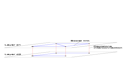
Figure 1: A two-layer multiplex network. Each layer is associated with one single decision variable. Blue lines represent social links between members, whereas dashed red lines represent the interconnections between the decisions of each member.

A multiplex network Multeplx1 ; Intro-MutiPlNet ; multi3 ; multi4 ; multi5 with $N$ different layers is defined. On each layer, individuals share their opinions on a certain decision variable $d_{j}$ leading to a certain level of conflict $E^{j}$. The graph of social network on the layer $d_{j}$ is described in terms of the symmetric adjacency matrix $\mathbf{A}^{j}$ with elements $A_{kh}^{j}$. The interconnections between different layers represent the interactions among the opinions of the same individual $k$ on the decision variables. Figure 1 shows an example of a multiplex network with only two layers, where the dashed lines connecting the different decision layers represent the interaction between the opinions that each member has on the decision variables. This interaction occurs via the $N-K$ perceived fitness, i.e. changing the opinion on the decision variable $j$ causes a modification of the perceived pay-off, which also depends on the opinions the member has on the remaining decision variables. In order to model the dynamics of decision-making in terms of a continuous-time Markov process, we define the state vector $\mathbf{s}$ of the entire group as $\mathbf{s=}\left(s_{1},s_{2},...,s_{n}\right)=\left(\sigma_{1}^{1},\sigma_{1}^{2},...\sigma_{1}^{N},\sigma_{2}^{1},\sigma_{2}^{2},...\sigma_{2}^{N},...,\sigma_{M}^{1},\sigma_{M}^{2},...\sigma_{M}^{N}\right)$ of size $n$ $=M\times N$, and the block diagonal adjacency matrix $\mathbf{A}=\mathrm{diag}\left(\mathbf{A}^{1},\mathbf{A}^{2},...,\mathbf{A}^{N}\right)$. For any given $l$-th component $s_{l}=\sigma_{k}^{j}$ of the vector $\mathbf{s}$ it is possible to uniquely identify the member $k$ and the decision variable $j$ by means of the relations $k=\mathrm{quotient}\left(l-1,M\right)+1$, and $j=\operatorname{mod}\left(l-1,M\right)+1$. The total level of conflict can be then rephrased as

$$E\left(\mathbf{s}\right)=-\frac{1}{2}J\mathbf{As\cdot s=}-\frac{1}{2}J\sum_{ij}A_{ij}s_{i}s_{j}$$ (4)

Observe that $A_{ii}=0$ (with $i=1,...,n$). In Eq. (4) the term $1/2$ avoids that each couple of members $k$ and $h$ be double counted. Now let be $P\left(\mathbf{s},t\right)$ the probability that, at time $t$, the state vector takes the value $\mathbf{s}$ out of $2^{n}$ possible states. The time evolution of the probability $P\left(\mathbf{s},t\right)$ obeys the master equation

$$\frac{dP\left(\mathbf{s},t\right)}{dt} =-\sum_{l}w\left(\mathbf{s}_{l}\rightarrow\mathbf{s}_{l}^{\prime}\right)P\left(\mathbf{s}_{l},t\right)$$ (5)

$$+\sum_{l}w\left(\mathbf{s}_{l}^{\prime}\rightarrow\mathbf{s}_{l}\right)P\left(\mathbf{s}_{l}^{\prime},t\right)$$

where $\mathbf{s}_{l}=\left(s_{1},s_{2},...,s_{l},...,s_{n}\right)$, $\mathbf{s}_{l}^{\prime}=\left(s_{1},s_{2},...,-s_{l},...,s_{n}\right)$. The transition rate $w\left(\mathbf{s}_{l}\rightarrow\mathbf{s}_{l}^{\prime}\right)$ is the probability per unit time that the opinion $s_{l}$ flips to $-s_{l}$ while the others remain temporarily fixed. Recalling that flipping of opinions is governed by social interactions and self-interest a possible ansatz for the transition rates is

$$w\left(\mathbf{s}_{l}\rightarrow\mathbf{s}_{l}^{\prime}\right) =\frac{1}{2}\left[1-s_{l}\tanh\left(\beta J\sum_{h}A_{lh}s_{h}\right)\right]$$ (6)

$$\times\exp\left\{\beta^{\prime}\left[\Delta V\left(\mathbf{s}_{l}^{\prime},\mathbf{s}_{l}\right)\right]\right\}$$

In Eq. (6) the pay-off function $\Delta V\left(\mathbf{s}_{l}^{\prime},\mathbf{s}_{l}\right)=\bar{V}\left(\mathbf{s}_{l}^{\prime}\right)-\bar{V}\left(\mathbf{s}_{l}\right)$, where $\bar{V}\left(\mathbf{s}_{l}\right)=V_{k}\left(\mathbf{\sigma}_{k}\right)$, is simply the change of the fitness perceived by the agent $k=\mathrm{quotient}\left(l-1,M\right)+1$, when its opinion $s_{l}=\sigma_{k}^{j}$ on the decision $j=\mathrm{\operatorname{mod}}\left(l-1,M\right)+1$ changes from $s_{l}=\sigma_{k}^{j}$ to $s_{l}^{\prime}=-\sigma_{k}^{j}$. The transition rates $w\left(\mathbf{s}_{l}\rightarrow\mathbf{s}_{l}^{\prime}\right)$ have been chosen to be the product of the transition rate of the Ising-Glauber dynamics Glauber (see also Appendix B), and the Weidlich exponential rate $\exp\left\{\beta^{\prime}\left[\Delta V\left(\mathbf{s}_{k}^{\prime},\mathbf{s}_{k}\right)\right]\right\}$weidlich2 ; Sweitzer . Note that Eq. (6) satisfies the detailed balance condition (see Appendix C). In Eq. (6) the quantity $\beta$ is the inverse of the so-called social temperature and is a measure of the chaotic circumstances, which lead to a random opinion change. The term $\beta^{\prime}$ is related to the degree of uncertainty associated with the information about the perceived fitness (the higher $\beta^{\prime}$ the less the uncertainty).

To solve the Markov process Eqs. (5, 6), we employ a simplified version of the exact stochastic simulation algorithm proposed by Gillespie Gillespie1 ; Gillespie2 . A brief summary of the algorithm is provided in Appendix D. The algorithm allows to generate a statistically correct trajectory of the stochastic process Eqs. (5, 6).

III Measuring the performance of the collective decision-making process

The group fitness value Eq. (1) and the level of agreement between the members (i.e. social consensus) are used to measure the performance of the collective-decision making process. To calculate the group fitness value, the vector $\mathbf{d=}\left(d_{1},d_{2},...,d_{N}\right)$ needs to be determined. To this end, consider the set of opinions $\left(\sigma_{1}^{j},\sigma_{2}^{j},...,\sigma_{M}^{j}\right)$ that the members of the group have about the decision $j$, at time $t$. The decision $d_{j}$ is obtained by employing the majority rule, i.e. we set

$$d_{j}=\mathrm{sgn}\left(M^{-1}\sum_{k}\sigma_{k}^{j}\right),\qquad j=1,2,...,N$$ (7)

If $M$ is even and in the case of a parity condition, $d_{j}$ is, instead, uniformly chosen at random between the two possible values $\pm 1$. The group fitness is then calculated as $V\left[\mathbf{d}\left(t\right)\right]$ and the ensemble average $\left\langle V\left(t\right)\right\rangle$ is then evaluated. The efficacy of the group in optimizing $\left\langle V\left(t\right)\right\rangle$ is then calculated in terms of normalized average fitness $\left\langle V\left(t\right)\right\rangle/V_{\max}$ where $V_{\max}=\max\left[V\left(\mathbf{d}\right)\right]$.

The consensus of the members on the decision variable $j$ is measured as follows. We define the average opinion $\bar{\sigma}^{j}$ of the group on the decision $j$

$$\bar{\sigma}^{j}=\frac{1}{M}\sum_{k}\sigma_{k}^{j}$$ (8)

Note that the quantity $\bar{\sigma}^{j}$ ranges in the interval $-1\leq\bar{\sigma}^{j}\leq 1$, and that $\bar{\sigma}^{j}=\pm 1$ only when full consensus is reached. Therefore, a possible measure of the consensus among the members on the decision variable $j$ is given by the ensemble average of the time-dependent quantity $C^{j}=\left(\bar{\sigma}^{j}\right)^{2}\in\left[0,1\right]$, i.e.,

$$\left\langle C^{j}\left(t\right)\right\rangle=\frac{1}{M^{2}}\sum_{kh}\left\langle\sigma_{k}^{j}\left(t\right)\sigma_{h}^{j}\left(t\right)\right\rangle=\frac{1}{M^{2}}\sum_{kh}R_{hk}^{j}\left(t\right)$$ (9)

Note that $\left\langle\sigma_{k}^{j}\left(t\right)\sigma_{h}^{j}\left(t\right)\right\rangle=R_{hk}^{j}\left(t\right)$ is the correlation function of the opinions of the members $k$ and $h$ on the same decision variable $j$. Given this, a possible ansatz to measure the entire consensus of the group on the whole set of decisions is

$$\left\langle C\left(t\right)\right\rangle=\frac{1}{N}\sum_{j}\left\langle C^{j}\left(t\right)\right\rangle=\frac{1}{M^{2}N}\sum_{j=1}^{N}\sum_{kh=1}^{M}R_{hk}^{j}\left(t\right)$$ (10)

Note that $0\leq\left\langle C\left(t\right)\right\rangle\leq 1$.

IV Simulation and results

We consider, unless differently specified, a group of $M=6$ members which have to make $N=12$ decisions. For the sake of simplicity, the network of social interactions on each decision layer $j$ is described by a complete graph, where each member is connected to all the others. We also set $\beta^{\prime}=10,$ since we assume that the information about the perceived fitness function is characterized by a low level of uncertainty. We simulate many diverse scenarios to investigate the influence of the parameter $p$, i.e. of the level of knowledge of the members, and the effect of the parameter $\beta J$ on the final outcome of the decision-making process. The simulation is stopped at steady-state. This condition is identified by simply taking the time-average of consensus and pay-off over consecutive time intervals of fixed length $T\$and by checking that the difference between two consecutive averages is sufficiently small.

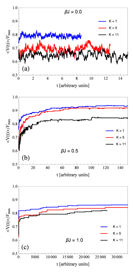
Figure 2: The time-evolution of the normalized average group fitness $\left\langle V\left(t\right)\right\rangle/V_{\max}$, for $p=0.5$, $K=1,5,11$. $\beta J=0.0$, (a); $\beta J=0.5$, (b); $\beta J=1.0$, (c).

For any given $p$ and $\beta J$, each stochastic process Eqs. (5, 6) is simulated by generating 100 different realizations (trajectories). For each single realization, the competence matrix $\mathbf{D}$ is set, and the initial state of the system is obtained by drawing from a uniform probability distribution, afterwards the time evolution of the state vector is calculated with the stochastic simulation algorithm (see Appendix D).

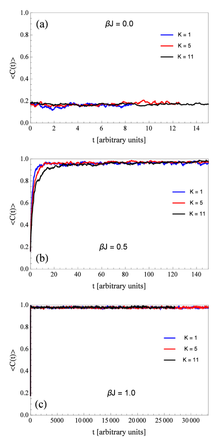
Figure 3: The time-evolution of the statistically averaged consensus $\left\langle C\left(t\right)\right\rangle$ for $p=0.5$, $K=1,5,11$. $\beta J=0.0$, (a); $\beta J=0.5$, (b); $\beta J=1.0$, (c).

Fig. 2 shows the time-evolution of normalized average fitness $\left\langle V\left(t\right)\right\rangle/V_{\max}$, for $p=0.5$ (i.e. for a moderate level of knowledge of the members), different values of the complexity parameter $K=1,5,11$, and different values of $\beta J=0.0,0.5,1.0$. We observe that for $\beta J=0$, i.e. in absence of social interactions [see Fig. 2(a)] the decision-making process is strongly inefficient, as witnessed by the very low value of the average fitness of the group. Each individual of the group makes his/her choices in order to optimize the perceived fitness, but, because of the absence of social interactions, he/she behaves independently from the others and does not receive any feedback about the actions of the other group members. Hence, individuals remain close to their local optima, group fitness cannot be optimized [see Fig. 2(a)], and the consensus is low [see Fig. 3(a)].

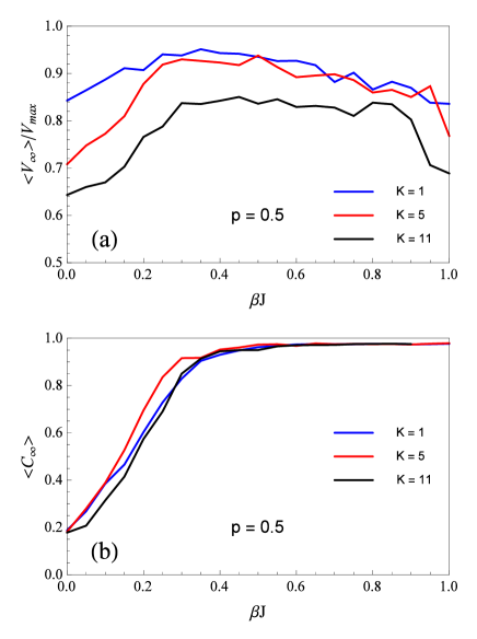
Figure 4: The stationary values of the normalized averaged fitness $\left\langle V_{\infty}\right\rangle/V_{\max}$ as a function of $\beta J$, (a); and of the statistically averaged consensus $\left\langle C_{\infty}\right\rangle$ as a function of $\beta J$, (b). Results are presented for $p=0.5$, $K=1,5,11$

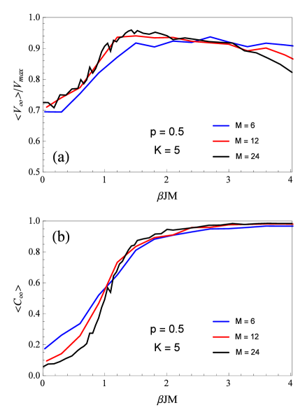
Figure 5: The stationary values of the normalized averaged fitness $\left\langle V_{\infty}\right\rangle/V_{\max}$ as a function of $M\beta J$, (a); and of the statistically averaged consensus $\left\langle C_{\infty}\right\rangle$ as a function of $M\beta J$, (b). Results are presented for $p=0.5$, $K=5$ and for three different team sizes: $M=6,12,24$.

As the strength of social interactions increases, i.e., $\beta J=0.5$ [Fig. 2(b)], members can exchange information about their choices. Social interactions push the individuals to seek consensus with the member who is experiencing higher payoff. In fact, on the average, those members, which find a higher increase of their perceived fitness, change opinion much faster than the others. Thus, the other members, in process of seeking consensus, skip the local optima of their perceived fitness and keep exploring the landscape, leading to a substantial increase of the group performance both in terms of group fitness values [Fig. 2(b)] as well as in terms of final consensus [Fig. 3(b)].

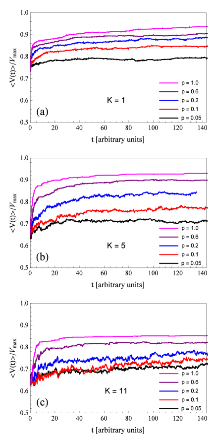
Figure 6: The time-evolution of the normalized average group fitness $\left\langle V\left(t\right)\right\rangle/V_{\max}$ for $\beta J=0.5$, $p=0.05,0.1,0.2,0.6,1$. $K=1$, (a); $\ K=5$, (b); $K=11$, (c).

Thus, the system collectively shows a higher level of knowledge and higher ability in making good choices than the single members (i.e., a higher degree of intelligence). It is noteworthy that when the strength of social interactions is too large, $\beta J=1$, [Fig. 2(c)] the performance of the group in terms of fitness value worsens. In fact, very high values of $\beta J$, accelerating the achievement of consensus among the members [Fig. 3(c)], significantly impede the exploration of the fitness landscape and hamper that change of opinions can be guided by payoff improvements.

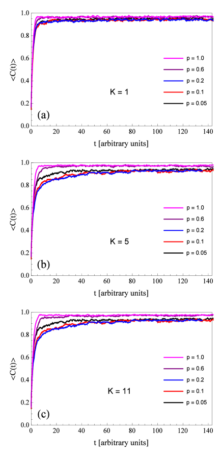
Figure 7: The time-evolution of the statistically averaged consensus $\left\langle C\left(t\right)\right\rangle$ for $\beta J=0.5$, $p=0.05,0.1,0.2,0.6,1$. $K=1$, (a); $\ K=5$, (b); $K=11$, (c).

The search of the optimum on the fitness landscape is slowed down, and the performance of the collective decision-making decreases both in terms of the time required to reach the steady-state as well as in terms of group fitness.

Figure 2 shows that rising the complexity of the landscape, i.e. increasing $K$, negatively affects the performance of the collective decision-making process, but does not qualitatively change the behavior of the system. However, Figure 2(b) also shows that, in order to cause a significant worsening of the group fitness, $K$ must take very large values, i.e., $K=11$. Instead, at moderate, but still significant, values of complexity (see results for $K=5$) the decision-making process is still very effective, leading to final group fitness values comparable to those obtained at the lowest level of complexity, i.e., at $K=1$.

In Figure 3 the ensemble average $\left\langle C\left(t\right)\right\rangle$ of the consensus among the members is shown as a function of time $t$, for $p=0.5$, $K=1,5,11$, and for different values of $\beta J=0.0,0.5,1.0$. At $\beta J=0$, the consensus is low.

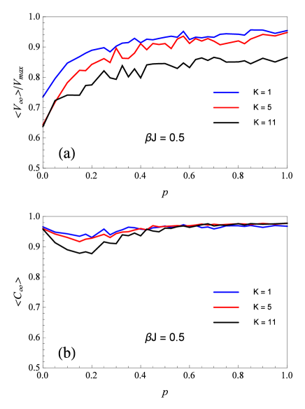
Figure 8: The stationary values of the normalized average group fitness $\left\langle V_{\infty}\right\rangle/V_{\max}$ as a function of $p$, (a); and of the statistically averaged consensus $\left\langle C_{\infty}\right\rangle$ as a function of $p$, (b). Results are presented for $\beta J=0.5$, $K=1,5,11$

In this case, at each time $t$, members’ opinions are random variables almost uniformly distributed between the two states $\pm 1$. Hence, the quantity $\left\langle C\left(t\right)\right\rangle$ can be analytically calculated as $\left\langle C\left(t\right)\right\rangle\approx 1/M$. For $M=6$ this gives $\left\langle C\left(t\right)\right\rangle\approx 0.16$, which is just the average value observed in Fig. 3(a). As the strength of social interactions rises, members more easily converge toward a common opinion. However, the random nature of the opinion dynamics still prevents full agreement from being achieved, see Fig. 3(b). This, as observed in Figure 2(b), has a very beneficial effect as individuals continue exploring the fitness landscape looking for maxima, thus leading to higher performance of the collective decision-making process. However, when the strength of social interactions is significantly increased, a very high value of consensus among members is rapidly achieved [see Fig. 3(c)], the exploration of the landscape is slowed down, and the performance of the decision making-process significantly worsen, see Figure 2(c). We, then, expect that, given $\beta^{\prime}$and $K$, a optimum of $\beta J$ exists, which maximizes the steady-state fitness of the group. This is, indeed, confirmed by the analysis shown in Figure 4, where the steady-state values of the normalized group fitness $\left\langle V_{\infty}\right\rangle/V_{\max}=\left\langle V\left(t\rightarrow\infty\right)\right\rangle/V_{\max}$ [Fig. 4(a)], and social consensus $\left\langle C_{\infty}\right\rangle=\left\langle C\left(t\rightarrow\infty\right)\right\rangle$ [Fig. 4(b)] are plotted as a function of $\beta J$, for $p=0.5$ and the three considered values of $K=1,5,11$. results in Figure 4(a) stresses that the fitness landscape complexity (i.e., the parameter $K$) marginally affects the performance of the decision-making process in terms of group fitness, provided that $K$ does not take too high values. In fact curves calculated for $K=1,5$ run close to each-other. More interesting, Figure 4 shows that increasing $\beta J$ from zero, makes both $\left\langle V_{\infty}\right\rangle/V_{\max}$ and $\left\langle C_{\infty}\right\rangle$ rapidly increase. This increment is, then, followed by a region of a slow change of $\left\langle V_{\infty}\right\rangle/V_{\max}$ and $\left\langle C_{\infty}\right\rangle$. It is worth noticing, that the highest group fitness value is obtained at the boundary between the increasing and almost stationary regions of $\left\langle C_{\infty}\right\rangle$. Moreover, results show that high consensus is necessary to guarantee high efficacy of the decision-making process, i.e. high values of $\left\langle V_{\infty}\right\rangle/V_{\max}$. This suggests that the decision making becomes optimal, i.e. the group as a whole is characterized by a higher degree of intelligence, at the point where the system dynamics changes qualitatively. This aspect of the problem is investigated in Figure 5 where the stationary values of normalized group-fitness and consensus are shown as a function of the quantity $\beta JM$ for different sizes $M=6,12,24$, for $N=12$ and $K=5$. Notably, the transition from low to high fitness values is always accompanied by an analogous transition from low to high consensus of the group. The transition becomes sharper and sharper as the group size $M$ is incremented. In all cases the transition occurs for $\beta JM\approx 1$. This value is particularly interesting as it can be easily shown, by using a mean-field approach (see Appendix E), that for large Ising systems $M\gg 1$ and in the case of complete graphs, the critical values $\left(\beta J\right)_{c}$, at which consensus sets in, satisfies the relation $\left(\beta J\right)_{c}=1/M$, in perfect agreement with our small-size numerical calculations. This is a very important result, which has analogies in many different self-organizing systems, as flocking systems and information flow processing Flocking 1 ; Flocking2 ; Info1 ; Info2 ; Info3 .

In Figure 6 we investigate the influence of the level of knowledge $p$ of members on the time-evolution of the normalized average fitness $\left\langle V\left(t\right)\right\rangle/V_{\max}$. Results are presented for $\beta J=0.5$, $K=1,5,11$, and for different values of $p=0.05,0.1,0.2,0.6,1.0$. Results show that improving the knowledge of the members, i.e. increasing $p$, enhances the performance of the decision-making process. In particular, a higher steady-state normalized fitness $\left\langle V_{\infty}\right\rangle/V_{\max}$, and a faster convergence toward the steady-state are observed. Note also, that, especially in the case of high complexity [Figure 6(b,c)], increasing $p$ above $0.2$ reduces the fluctuations of $\left\langle V\left(t\right)\right\rangle$, as a consequence of the higher agreement achieved among the members at higher level of knowledge. This is clear in Figure 7, where the time-evolution of the consensus $\left\langle C\left(t\right)\right\rangle$ is shown for $\beta J=0.5$, $K=1,5,11$, and $p=0.05,0.1,0.2,0.6,1.0$. In Figure 8 the steady-state values of the normalized group fitness $\left\langle V_{\infty}\right\rangle/V_{\max}$ [Fig. 8(a)], and social consensus $\left\langle C_{\infty}\right\rangle$ [Fig. 8(b)] are shown as a function of $p$, for $\beta J=0.5$ and the three considered values of $K=1,5,11$. Note that as $p$ is increased from zero, the steady state value $\left\langle V_{\infty}\right\rangle/V_{\max}$ initially grows fast [Fig. 8(a)]. In fact, because of social interactions, increasing the knowledge of each member also increases the knowledge of the group as a whole. But, above a certain threshold of $p$ the increase of $\left\langle V_{\infty}\right\rangle/V_{\max}$ is much less significant. This indicates that the knowledge of the group is subjected to a saturation effect. Therefore, a moderate level of knowledge is already enough to guarantee very good performance of decision-making process, higher knowledge levels being only needed to accelerate the convergence of the decision-making process. Figure 8(b) shows that for vanishing values of $p$ the consensus $\left\langle C_{\infty}\right\rangle$ takes high values, as each member’s choice is driven only by consensus seeking. Increasing $p$ initially causes a decrease of consensus, as the self-interest of each member leads to a certain level of disagreement. However, a further increment of $p$ makes the members’ knowledge overlap so that the self-interest of each member almost points in the same direction, resulting in a consensus increase.

V Conclusions

In this paper we developed a model of collective decision-making in human groups in presence of complex environment. The model described the time evolution of group choices in terms of a time-continuous Markov process, where the transition rates have been defined so as to capture the effect of the two main forces, which drive the change of opinion of the members of the group. These forces are the rational behavior which pushes each member to increase his/her self-interest, and the social interactions, which push the members to reach a common opinion. Our study provides contribution to the literature identifying under which circumstances collective decision making is more performing. We found that a moderate strength of social interactions allows for knowledge transfer among the members, leading to higher knowledge level of the group as a whole. This mechanism, coupled with the ability to explore the fitness landscape, strongly improves the performance of the decision-making process. In particular we found that the threshold value of the social interaction strength, at which the entire group behaves as unique entity characterized by a higher degree of intelligence, is just the critical threshold at which the consensus among the members sets in. This value can be also calculated for large systems trough mean-field techniques and results to be in perfect agreement with our small system calculations. One can therefore estimate for any given social temperature $\beta^{-1}$ and social interaction strength $J$ the optimal number $M_{\mathrm{opt}}\approx\left(\beta J\right)^{-1}$ of team members leading to the emergence of a superior intelligence of the group.

We also found that increasing the level of knowledge of the members improves performance. However, above a certain threshold the knowledge of the group saturates, i.e. the performance of the collective decision-making process becomes much less sensitive to the level of knowledge of each single member. Therefore, we can state that the collective decision-making is very high-performing already at moderate level of knowledge of the members, and that very high knowledge of all members only serves to accelerate the convergence of the decision-making process. Our results also showed that human groups with optimal levels of members’ knowledge and strength of social interactions very well manage complex problems.

Appendix A The $N-K$ fitness landscape generation

In the $N-K$ model a real valued fitness is assigned to each bit string $\mathbf{d=}\left(d_{1},d_{2},...,d_{N}\right)$, where $d_{i}=\pm 1$. This is done by first assigning a real valued contribution $W_{i}$ to the $i$-th bit $d_{i}$, and then by defining the fitness function as $V\left(\mathbf{d}\right)=N^{-1}\sum_{j=1}^{N}W_{j}\left(d_{j},d_{1}^{j},d_{2}^{j},..,d_{K}^{j}\right)$. Each contribution $W_{i}$ depends not just on $i$ and $d_{i}$ but also on $K$ ($0\leq K<N$) other bits. Now let us define the substring $\mathbf{s}_{i}=\left(d_{i},d_{1}^{i},d_{2}^{i},..,d_{K}^{i}\right)$, by chosing at random, for each bit $i$, $K$ other bits. Each single contribution $W_{i}\left(\mathbf{s}_{i}\right)$ is then a random function of $2^{K+1}$ possible values of $\mathbf{s}_{i}$, and its value is drawn from a uniform distribution. Thus, a random table of contributions is generated independently for each $i$-th bit, thus allowing the calculate of the fitness function $V\left(\mathbf{d}\right)$. The reader is referred to Refs. NK-model ; NK-model1 ; NK-model2 for more details on the $N-K$ complex landscapes.

Appendix B The Glauber dynamics on general graphs

Consider the Ising model on a general graph with adjacency matrix $A_{ij}$. The total energy of the system is given in Eq. (4). In steady state conditions the stationary distribution of the probability of the states $P_{0}\left(\mathbf{s}\right)$ is given by the Boltzmann distribution

$$P_{0}\left(\mathbf{s}\right)=\frac{\exp\left[-\beta E\left(\mathbf{s}\right)\right]}{Z}$$ (11)

where $Z=\sum_{l}\exp\left[-\beta E\left(\mathbf{s}_{l}\right)\right]$ is the partition function of the system. The detailed balance condition then requires that

$$\frac{w\left(\mathbf{s}_{l}\rightarrow\mathbf{s}_{l}^{\prime}\right)}{w\left(\mathbf{s}_{l}^{\prime}\rightarrow\mathbf{s}_{l}\right)}=\frac{P_{0}\left(\mathbf{s}_{l}^{\prime}\right)}{P_{0}\left(\mathbf{s}_{l}\right)}=\frac{\exp\left[-\beta E\left(\mathbf{s}_{l}^{\prime}\right)\right]}{\exp\left[-\beta E\left(\mathbf{s}_{l}\right)\right]}$$ (12)

Now observe that

$$E\left(\mathbf{s}_{l}\right)=-Js_{l}\sum_{j}A_{lj}s_{j}-\frac{1}{2}J\sum_{ij\neq l}A_{ij}s_{i}s_{j}$$ (13)

Substituting Eqs. (13) in Eq. (12) and recalling that $\exp\left(x\right)=\cosh\left(x\right)+\sinh\left(x\right)$ we get

$$\frac{w\left(\mathbf{s}_{l}\rightarrow\mathbf{s}_{l}^{\prime}\right)}{w\left(\mathbf{s}_{l}^{\prime}\rightarrow\mathbf{s}_{l}\right)}=\frac{1-\tanh\left(\beta Js_{l}\sum_{j}A_{lj}s_{j}\right)}{1+\tanh\left(\beta Js_{l}\sum_{j}A_{lj}s_{j}\right)}$$ (14)

Noting that $s_{l}=\pm 1$, so that $\tanh\left(\beta Js_{l}\sum_{j}A_{lj}s_{j}\right)=s_{l}\tanh\left(\beta J\sum_{j}A_{lj}s_{j}\right)$ we finally obtain

$$\frac{w\left(\mathbf{s}_{l}\rightarrow\mathbf{s}_{l}^{\prime}\right)}{w\left(\mathbf{s}_{l}^{\prime}\rightarrow\mathbf{s}_{l}\right)}=\frac{1-s_{l}\tanh\left(\beta J\sum_{j}A_{lj}s_{j}\right)}{1+s_{l}\tanh\left(\beta J\sum_{j}A_{lj}s_{j}\right)}$$ (15)

Therefore, a possible choice for the transition rates for the Ising-Glauber dynamics on general graph is

$$w\left(\mathbf{s}_{l}\rightarrow\mathbf{s}_{l}^{\prime}\right)=\alpha\left[1-s_{l}\tanh\left(\beta J\sum_{j}A_{lj}s_{j}\right)\right]$$ (16)

where $\alpha$ is an arbitrary constant. We have chosen $\alpha=1/2$.

Appendix C Detailed balance condition

Here we show that the transition rate given in Eq. (6) fulfils the detailed balance condition of Markov chains, which requires the existence of a stationary probability distribution $P_{0}\left(\mathbf{s}_{l}\right)$ such that

$$\frac{P_{0}\left(\mathbf{s}_{l}^{\prime}\right)}{P_{0}\left(\mathbf{s}_{l}\right)}=\frac{w\left(\mathbf{s}_{l}\rightarrow\mathbf{s}_{l}^{\prime}\right)}{w\left(\mathbf{s}_{l}^{\prime}\rightarrow\mathbf{s}_{l}\right)}$$ (17)

Using Eq. (6) the above condition Eq. (17) writes

$$\frac{P_{0}\left(\mathbf{s}_{l}^{\prime}\right)}{P_{0}\left(\mathbf{s}_{l}\right)} =\frac{1-s_{l}\tanh\left(\beta J\sum_{h}A_{lh}s_{h}\right)}{1+s_{l}\tanh\left(\beta J\sum_{h}A_{lh}s_{h}\right)}$$ (18)

$$\times\frac{\exp\left\{\beta^{\prime}\left[\bar{V}\left(\mathbf{s}_{l}^{\prime}\right)-\bar{V}\left(\mathbf{s}_{l}\right)\right]\right\}}{\exp\left\{\beta^{\prime}\left[\bar{V}\left(\mathbf{s}_{l}\right)-\bar{V}\left(\mathbf{s}_{l}^{\prime}\right)\right]\right\}}$$

and recalling Eqs. (12, 15) yields

$$\frac{P_{0}\left(\mathbf{s}_{l}^{\prime}\right)}{P_{0}\left(\mathbf{s}_{l}\right)}=\frac{\exp\left[-\beta E\left(\mathbf{s}_{l}^{\prime}\right)+2\beta^{\prime}\bar{V}\left(\mathbf{s}_{l}^{\prime}\right)\right]}{\exp\left[-\beta E\left(\mathbf{s}_{l}\right)+2\beta^{\prime}\bar{V}\left(\mathbf{s}_{l}\right)\right]}$$ (19)

this allows to define the stationary probability distribution

$$P_{0}\left(\mathbf{s}_{l}\right)=\frac{\exp\left[-\beta E\left(\mathbf{s}_{l}\right)+2\beta^{\prime}\bar{V}\left(\mathbf{s}_{l}\right)\right]}{\sum_{k}\exp\left[-\beta E\left(\mathbf{s}_{k}\right)+2\beta^{\prime}\bar{V}\left(\mathbf{s}_{k}\right)\right]}$$ (20)

which satisfies the detailed balance condition Eq. (17).

Appendix D The stochastic simulation algorithm

The stochastic simulation algorithm we use to solve the Markov process (5) is derived from the one proposed by Gillespie Gillespie1 ; Gillespie2 . We just summarize the main steps of the algorithm:

1. Choose a random initial state $\mathbf{s}$ of the system

2. Calculate the transition rates $w\left(\mathbf{s}_{l}\rightarrow\mathbf{s}_{l}^{\prime}\right)$

3. Calculate the total rate $w_{T}=\sum_{l}w\left(\mathbf{s}_{l}\rightarrow\mathbf{s}_{l}^{\prime}\right)$

4. Normalize the transition rates as $\nu_{l}=w\left(\mathbf{s}_{l}\rightarrow\mathbf{s}_{l}^{\prime}\right)/w_{T}$

5. Construct the cumulative distribution $F\left(\nu_{l}\right)$ from the probability mass function $\nu_{l}$

6. Calculate the time $\Delta t$ to the next opinion flip drawing from an exponential distribution with mean $1/w_{T}$, i.e. choose a real random number $0\leq r<1$ from a uniform distribution and set $\Delta t=-w_{T}^{-1}\log\left(r\right)$.

7. Identify the $k$-th opinion $s_{k}$ which flips from $s_{k}$ to $-s_{k}$ by drawing from a discrete distribution with probability mass function $\nu_{l}$, i.e. draw a real random number $0\leq s<1$ from a uniform distribution and choose $k$ so that $F\left(\nu_{k-1}\right)\leq s<F\left(\nu_{k}\right)$.

8. Update the state vector and return to step 2 or quit.

Appendix E The mean-field calculations of the Ising model on a complete graph.

On a complete graph the total energy of a system of $M$ spins is

$$E=-\sum_{k<h}J\sigma_{k}\sigma_{h}$$ (21)

and the average magnetization is $\left\langle\sigma\right\rangle=M^{-1}\sum_{k}\left\langle\sigma_{k}\right\rangle$. Using Eq. (16) the Ising-Glauber rate becomes

$$w_{k}=w\left(\sigma_{k}\rightarrow-\sigma_{k}\right)=\frac{1}{2}\left[1-\sigma_{k}\tanh\left(\beta J\sum_{j\neq k}\sigma_{j}\right)\right]$$ (22)

Using Eq. (5) one can easily derive the following equation of motion for the average magnetization $\left\langle\sigma_{k}\right\rangle$ of the $k$-th site

$$\frac{d\left\langle\sigma_{k}\right\rangle}{dt}=-2\left\langle w_{k}\sigma_{k}\right\rangle=-\left\langle\sigma_{k}\right\rangle+\left\langle\tanh\left(\beta J\sum_{j}\sigma_{j}\right)\right\rangle$$ (23)

Assuming that $M$ is large, using $\left\langle\sigma\right\rangle=M^{-1}\sum_{k}\left\langle\sigma_{k}\right\rangle$, and exploiting the mean field approach we write $\left\langle\tanh\left[\beta J\sum_{j}\sigma_{j}\right]\right\rangle=\tanh\left[\beta J\sum_{j}\left\langle\sigma_{j}\right\rangle\right]=\tanh\left[\left\langle\sigma\right\rangle\beta JM\right]$, and

$$\frac{d\left\langle\sigma\right\rangle}{dt}=-\left\langle\sigma\right\rangle+\tanh\left[\left\langle\sigma\right\rangle\beta JM\right]$$ (24)

The average magnetization $\left\langle\sigma\right\rangle$ at the fixed point of Eq. (24) satisfies the relation

$$\left\langle\sigma\right\rangle=\tanh\left[\left\langle\sigma\right\rangle M\beta J\right]$$ (25)

For $M\beta J\leq 1$ only the trivial solution $\left\langle\sigma\right\rangle_{1}=0$ can be found. However, for $M\beta J>1$ other two solutions $\left\langle\sigma\right\rangle_{2}=-\left\langle\sigma\right\rangle_{3}>0$ appear which depends on the specific value of $M\beta J$. In this case $\left\langle\sigma\right\rangle_{1}=0$ becomes unstable. Thus, the critical point for the phase transition is

$$\left(\beta J\right)_{c}=\frac{1}{M}$$ (26)

The above equation is in perfect agreement with the results shown in Fig. 5, thus confirming that the decision making process of the group becomes optimal just when the system changes qualitatively its dynamics.

References

- (1) Conradt L., Roper T. J., Group decision-making in animals, Nature 421, 155-158, doi:10.1038/nature01294, 2003.
- (2) Couzin I.D., Krause J., Franks N.R., Levin S.A., Effective leadership and decision-making in animal groups on the move, Nature 433, 513-516, doi:10.1038/nature03236, 2005.
- (3) Krieger M.J.B., Billeter J-B., Keller L., Ant-like task allocation and recruitment in cooperative robots, Nature 406, 992-995, doi:10.1038/35023164, 2000.
- (4) Rubenstein M., Cornejo A., Nagpal R., Programmable self-assembly in a thousand-robot swarm, Science 345 (6198), 795-799, doi: 10.1126/science.1254295, 2014.
- (5) Werfel J., Petersen K., Nagpal R., Designing Collective Behavior in a Termite-Inspired Robot Construction Team, Science, 343 (6172), 754-758, doi: 10.1126/science.1245842, 2014.
- (6) Brambilla M., Ferrante E., Birattari M., Dorigo M., Swarm robotics: a review from the swarm engineering perspective, Swarm Intell 7,1–41, doi:10.1007/s11721-012-0075-2, 2013.
- (7) Ching Hua Lee and Andrew Lucas, Simple model for multiple-choice collective decision making, Phys. Rev. E 90, 052804 (2014)
- (8) Brummitt C.D., Chatterjee S., Dey P.S., Sivakoff D., Jigsaw percolation: What social networks can collaboratively solve a puzzle?, The Annals of Applied Probability 25(4), 2013-2038, doi: 10.1214/14-AAP1041, 2015.
- (9) Clément RJG, Krause S, von Engelhardt N, Faria JJ, Krause J, Kurvers RHJM, Collective Cognition in Humans: Groups Outperform Their Best Members in a Sentence Reconstruction Task. PLoS ONE 8(10), e77943, doi:10.1371/journal.pone.0077943, 2013
- (10) Galam S., Rational group decision making: A random field Ising model at T=0, PhysicaA 238, 66-80, (1997)
- (11) Galam S. Martins. A.C.R., Two-dimensional Ising transition through a technique from two-state opinion-dynamics models, Physical Review E 91, 012108 (2015)
- (12) Couzin I.D., Collective cognition in animal groups, Trends Cogn Sci., 13(1), 36-43, doi: 10.1016/j.tics.2008.10.002, 2009.
- (13) Sumpter D.J.T., Pratt S.C., Quorum responses and consensus decision making, Phil. Trans. R. Soc. B 364, 743–753, doi:10.1098/rstb.2008.0204 (2009)
- (14) Ward A.J.W., Sumpter D.J.T., Couzin I.D., Hart P.J.B., Krause J., Quorum decision-making facilitates information transfer in fish shoals, PNAS, 105 (19), 6948–6953, doi: 10.1073pnas.0710344105, 2008
- (15) Arganda S., Pérez-Escudero A., de Polavieja G.G., A common rule for decision making in animal collectives across species, PNAS, 109 (50), 20508–20513, 2012.
- (16) Ward A.J.W., Herbert-Read J.E., Sumpter D.J.T, Krause J., Fast and accurate decisions through collective vigilance in fish shoals, PNAS, 108 (6), 2312–2315, doi: 10.1073/pnas.1007102108, 2011.
- (17) Pérez-Escudero A, de Polavieja GG, Collective Animal Behavior from Bayesian Estimation and Probability Matching. PLoS Comput Biol 7(11), e1002282, doi:10.1371/journal.pcbi.1002282, 2011.
- (18) Watts D.J., A Simple Model of Global Cascades on Random Networks, PNAS, 99(9), 5766-5771, doi: 10.1 073/pnas.082090499, 2002.
- (19) Turalska M., Lukovic M., West B. J., Grigolini P., Complexity and synchronization, Phys. Rev. E 80, 021110, doi: 10.1103/PhysRevE.80.021110, 2009.
- (20) Wang, Z., Szolnoki, A., Perc, M., Optimal interdependence between networks for the evolution of cooperation, Scientific Reports, 3, 2470, DOI: 10.1038/srep02470, 2013.
- (21) Wang, Z., Szolnoki, A., Perc, M., Interdependent network reciprocity in evolutionary games, Scientific Reports, 3, 1183, DOI: 10.1038/srep01183, 2013.
- (22) Bonabeau E, Dorigo M., Theraulaz G., Inspiration for optimization from social insect behaviour, Nature 406, 39-42, doi:10.1038/35017500, 2000.
- (23) Garnier S., Gautrais J., Theraulaz G., The biological principles of swarm intelligence, Swarm Intell, 1, 3–31, doi: 10.1007/s11721-007-0004-y, 2007
- (24) Vanni F., Luković M., Grigolini P., Phys. Rev. Lett. 107, 078103, doi: 10.1103/PhysRevLett.107.078103, 2011.
- (25) Easley D, Kleinberg J, Networks, Crowds, and Markets: Reasoning About a Highly Connected World. Cambridge University Press, (2010)
- (26) Levinthal D.A., Adaptation on Rugged Landscapes, Management Science, 43 (7), 934-950, 1997
- (27) Katila R. Ahuja G., Something old, something new: A longitudinal study of search behavior and new product introduction, Academy of Management Journal, 45(6), 1183-1194, 2002.
- (28) Loch C., Mihm J., Huchzermeier A., Concurrent Engineering and Design Oscillations in Complex Engineering Projects, Concurrent Engineering September 11 (3), 187-199, doi: 10.1177/106329303038030, 2003.
- (29) Billinger S., Stieglitz N., Schumacher T.R., Search on Rugged Landscapes: An Experimental Study, Organization Science, 25 (1), 93-108, doi: 10.1287/orsc.2013.0829, 2014.
- (30) Turalska M., and West B. J., Imitation versus payoff: Duality of the decision-making process demonstrates criticality and consensus formation, Phys. Rev. E 90, 052815, doi: http://dx.doi.org/10.1103/PhysRevE.90.052815, 2014
- (31) Conradt L., Models in animal collective decisionmaking: information uncertainty and conflicting preferences, Interface Focus 2, 226–240 doi:10.1098/rsfs.2011.0090, 2012.
- (32) DiMaggio, P. J. and Powell, W. W., The iron cage revisited: Institutional isomorphism and collective rationality in organizational fields. American sociological review, 48(2) 147-160, 1983
- (33) Castellano C., Fortunato S., Loreto V., Statistical physics of social dynamics, Rev. Mod. Phys. 81 (2), 591, doi:10.1103/RevModPhys.81.591, 2009
- (34) Glauber R.J., Time-Dependent Statistics of the Ising Model, J. Math. Phys. 4, 294-307, doi: 10.1063/1.1703954, 1963.
- (35) Kauffman S., Levin S., Towards a general theory of adaptive walks on rugged landscapes, Journal of Theoretical Biology, 128 (1), 11–45, doi: 10.1016/S0022-5193(87)80029-2,1987
- (36) Kauffman, S.; Weinberger, E., The NK Model of rugged fitness landscapes and its application to the maturation of the immune response, Journal of Theoretical Biology, 141 (2), 211–245, doi:10.1016/s0022-5193(89)80019-0, 1989.
- (37) E. D. Weinberger, NP Completeness of Kauffman’s N-k Model, a Tuneably Rugged Fitness Landscape, Santa Fe Institute working paper: 1996-02-003, http://www.santafe.edu/media/workingpapers/96-02-003.pdf, 1996.
- (38) Sornette D., Physics and financial economics (1776–2014): puzzles, Ising and agent-based models, Rep. Prog. Phys. 77, 062001, doi:10.1088/0034-4885/77/6/062001, 2014.
- (39) Weidlich, W., The statistical description of polarization phenomena in society, British Journal of Mathematical and Statistical Psychology, 24 (2), 251-266, doi: 10.1111/j.2044-8317.1971.tb00470,1971.
- (40) Ising E., Beitrag zur Theorie des Ferromagnetismus, Zeitschrift für Physik, 31 (1), pp 253-258, doi: 10.1007/BF02980577, 1925
- (41) Brush S.G., History of the Lenz-Ising Model, Rev. Mod. Phys. 39, 883, doi: 10.1103/RevModPhys.39.883, 1967
- (42) Weidlich W., Physics and Social Science - the Approach of Synergetics, Physics Reports 204 (1), 1-163, 1991
- (43) Schweitzer F., Brownian Agents and Active Particles, Collective Dynamics in the Natural and Social Sciences, Springer Series in Synergetics - Springer Complexity, Springer, Berlin-Heidelberg-New York, isbn: 978-3540738442, 2007.
- (44) Gruènbaum D., Schooling as a strategy for taxis in a noisy environment, Evolutionary Ecology 12, 503-522, 1998.
- (45) Laughlin PR, Hatch EC, Silver JS, Boh L, Groups perform better than the best individuals on letters-to-numbers problems: effects of group size. J Pers Soc Psychol, 90, 644-651, doi: 10.1037/0022-3514.90.4.644, 2006
- (46) Laughlin PR, Zander ML, Knievel EM, Tan TK, Groups perform, better than the best individuals on letters-to-numbers problems: Informative equations and effective strategies. J Pers Soc Psychol, 85, 684-694, doi:10.1037/0022-3514.85.4.684, 2003.
- (47) Faria JJ, Codling EA, Dyer JRG, Trillmich F, Krause J, Navigation in human crowds; testing the many-wrongs principle. Anim Behav 78, 587-591, doi:10.1016/j.anbehav.2009.05.019, 2009
- (48) Dorigo M, Maniezzo V., Colorni A., The Ant System: Optimization by a colony of cooperating agents, IEEE Transactions on Systems, Man, and Cybernetics–Part B, 26 (1), 1-13, 1996.
- (49) Dorigo,M. & Gambardella, L. M. Ant colonies for the traveling salesman problem. BioSystems 43, 73-81 (1997).
- (50) Kennedy, J.; Eberhart, R., Particle Swarm Optimization, Proceedings of IEEE International Conference on Neural Networks. IV. pp. 1942–1948, 1995
- (51) Karaboga D. , Basturk B., A powerful and efficient algorithm for numerical function optimization: artificial bee colony (ABC) algorithm, Journal of Global Optimization 39, 459–471, 2007.
- (52) Li X., Shao Z., Qian J.,Anoptimizing method base on autonomous animates: fish- swarm algorithm, Systems, Engineering Theory and Practice 22, 32–38, 2002.
- (53) De Domenico M., Solé-Ribalta A., Cozzo E., Kivelä M., Moreno Y., Porter M.A., Gómez S., Arenas A., Mathematical Formulation of Multilayer Networks, Phys. Rev. X 3, 041022, doi:http://dx.doi.org/10.1103/PhysRevX.3.041022, 2013
- (54) Lee KM, Min B., Goh K., Towards real-world complexity: an introduction to multiplex networks, Eur. Phys. J. B, 88, 48, doi: 10.1140/epjb/e2015-50742-1, 2015.
- (55) Boccaletti, S., Bianconi, G., Criado, R., del Genio, C.I., Gómez-Gardeñes, J., Romance, M., Sendiña-Nadal, I., Wang, Z., Zanin, M., The structure and dynamics of multilayer networks, Physics Reports, 544 (1), 1-122, DOI: 10.1016/j.physrep.2014.07.001, 2014.
- (56) Wang, Z., Wang, L., Szolnoki, A., Perc, M. Evolutionary games on multilayer networks: a colloquium, European Physical Journal B, 88 (5), 1-15, DOI: 10.1140/epjb/e2015-60270-7, 2015.
- (57) Kivelä M., Arenas A., Barthelemy M., Gleeson J. P., Moreno Y., Porter M.A., Multilayer networks, Journal of Complex Networks 2, 203–271, doi:10.1093/comnet/cnu016, 2014.
- (58) Gillespie, D.T., A General Method for Numerically Simulating the Stochastic Time Evolution of Coupled Chemical Reactions, Journal of Computational Physics 22 (4), 403–434, doi:10.1016/0021-9991(76)90041-3, 1976.
- (59) Gillespie D.T., Exact Stochastic Simulation of Coupled Chemical Reactions, The Journal of Physical Chemistry, 81 (25), 2340–2361, doi:10.1021/j100540a008, 1977.
- (60) Vicsek T., Czirók A., Ben-Jacob E., Cohen I., Shochet O., Novel Type of Phase Transition in a System of Self-Driven Particles, Phys. Rev. Lett. 75, 1226, doi: http://dx.doi.org/10.1103/PhysRevLett.75.1226, 1995.
- (61) Vicseka T., Zafeirisa A., Collective motion, Physics Reports, 517 (3–4), 71–140, doi: 10.1016/j.physrep.2012.03.004, 2012.
- (62) Barnett L., Lizier J.T., Harré M., Seth A.K., Bossomaier T., Physical Review Letters, 111, 177203, doi:10.1103/PhysRevLett.111.177203, 2013
- (63) Kinouchi O.,Copelli M., Optimal dynamical range of excitable networks at criticality, Nature Physics 2, 348 - 351, doi:10.1038/nphys289, 2006
- (64) Mora T., Bialek W., Are Biological Systems Poised at Criticality?, J Stat Phys 144, 268–302, doi: 10.1007/s10955-011-0229-4, 2011