Tomograms for open quantum systems: in(finite) dimensional optical and spin systems

Abstract

Tomograms are obtained as probability distributions and are used to reconstruct a quantum state from experimentally measured values. We study the evolution of tomograms for different quantum systems, both finite and infinite dimensional. In realistic experimental conditions, quantum states are exposed to the ambient environment and hence subject to effects like decoherence and dissipation, which are dealt with here, consistently, using the formalism of open quantum systems. This is extremely relevant from the perspective of experimental implementation and issues related to state reconstruction in quantum computation and communication. These considerations are also expected to affect the quasiprobability distribution obtained from experimentally generated tomograms and nonclassicality observed from them.

I Introduction

A quantum state can be characterized by a number of probability and quasiprobability distribution functions st-est . The quasiprobability distributions are not true probability distributions as most of them can have nonpositive values. Interestingly, this nonpositivity can be viewed as a signature of nonclassicality or quantumness. Specifically, the negative values of the Wigner wig and $P$ glaub ; sudar functions serve as witnesses of nonclassicality. Further, zeros of $Q$ function comment1 also serve as witness of nonclassicality. As there does not exist any straight forward prescription for direct measurement of these quasiprobability distributions, several efforts have been made to construct measurable probability distributions that can be used to uniquely construct either all or some of these quasiprobability distributions. Such measurable probability distributions are referred to as tomograms tom-review ; with-adam ; manko-fss ; manko-spin-tom . In other words, the tomogram is a scheme for measuring a quantum state by using a representation in one to one correspondence with the true probability distribution rather than with a quasidistribution comment13-ref1 . A relationship between a tomogram and a quasidistribution function, such as the Wigner function, can be established for both continuous and discrete systems op-tom ; fss-tom . Specifically, in Ref. op-tom it was shown that quasiprobability distributions ($P$, $Q$, and Wigner functions) can be uniquely determined in terms of probability distributions for the rotated quadrature phase which can be viewed as an optical tomogram of the state. Similarly, in Ref. fss-tom it was shown that for finite dimensional phase states, discrete Wigner functions and tomograms are connected by a discretization of the continuous variable Radon transformation and was referred to as the Plato transformation.

In the recent past, a few successful attempts have been made to measure Wigner function directly in experiments wig-exp ; wig-exp2 , but the methods adopted are state specific. The same limitation is also valid for the theoretical proposals wig-diff for the measurement of Wigner function. Further, optical homodyne tomography has been employed for the experimental measurement of the Wigner functions of vacuum and squeezed states in comment5exp-ref1 ; comment5exp-ref2 , while distributions corresponding to Pegg-Barnett and Susskind-Glogower phase operators were also obtained in comment5exp-ref2 . An experimental measurement of the $P$, $Q$ and Wigner quantum phase distributions for the squeezed vacuum state has been reported in comment5exp-ref3 . Precision of homodyne tomography technique was compared with conventional detection techniques in comment5theory-ref1 . A number of alternative methods of tomography have also been proposed comment5theory-ref2 ; comment5theory-ref4 ; comment5theory-ref5 , and exploited to obtain phase distributions like Wigner and $Q$ functions comment5theory-ref3 . In CV-rev continuous variable quantum state tomography was reviewed from the perspective of quantum information. In brief, there does not exist any general prescription for direct experimental measurement of the Wigner function and other quasidistribution functions. In practice, to detect the nonclassicality in a system the Wigner function is obtained either by photon counting or from experimentally measured tomograms wig-diff . Thus, tomograms are very important for the identification of nonclassical character of a physical system. In another line of studies, simulation of quantum systems have been performed using tomography. For example, tomograms were used for simulation of tunneling comment9-ref1 ; comment9-ref2 ; comment9-ref4 and multimode quantum states comment9-ref3 . Attempts have also been made to understand the tomogram via path integrals comment9-ref5 ; comment9-ref6 .

Furthermore, how to reconstruct a quantum state from experimentally measured values is of prime interest for both quantum computation wig-exp and communication tel-143 . Specifically, in Ref. wig-exp it is strongly established that tomography and spectroscopy can be interpreted as dual forms of quantum computation, and in Ref. tel-143 , quantum teleportation was experimentally performed over a distance of 143 km and the quality of teleportation was verified with the help of quantum process tomography (QPT) of quantum teleportation without feed-forward. Here it would be apt to note that QPT is an aspect of quantum state tomography in which a quantum process is obtained as a trace preserving positive linear map QPT . In the recent past, quantum process tomography has been discussed from the perspective of open quantum system effects QPT-open ; marzolino1 ; marzolino2 . A novel method of complete experimental characterization of quantum optical processes was introduced in comment8-ref1 . It was further developed in comment8-ref2 ; comment8-ref3 and extended to characterization of $N$-modes in comment8-ref7 . In comment8-ref4 , QPT was applied to the characterization of optical memory based on electromagnetically induced transparency while comment8-ref5 and comment8-ref6 were devoted to QPT of the electromagnetic field and conditional state engineering, respectively. Quantum state tomography has its applications in quantum cryptography as well tom-cryp . Specifically, in Ref. tom-cryp an interesting protocol of quantum cryptography was proposed in which eavesdropping in the quantum channel was checked by requiring consistency of outcome of the tomography with the unbiased noise situation. Keeping these facts in mind, we aim to construct tomograms for a number of physical systems of practical relevance (mostly having applications in quantum computation and communication) and investigate the effects of various types of noise on them.

From the experimental perspective, a quantum state always interacts with its surroundings. Hence, the evolution of the corresponding tomogram after taking into account the interaction of the quantum state with its environment should be considered. This can be achieved with the open quantum system formalism louis ; bp ; pi ; sbqbm . Specifically, both purely dephasing (QND) QND and dissipative SGAD open quantum system effects have been studied here. Interestingly, both these effects have also been experimentally realized in the recent past haroche ; turchette . In Ref. our-qd-paper , a systematic study of quasidistribution functions was made for a host of interesting states under general open system evolutions.

Here, we set ourselves the task of obtaining the tomograms for various finite and infinite dimensional quantum systems in different open quantum system scenarios. For finite dimensional spin states, the tomogram is the distribution function of the projections of the spin on an arbitrary axis, characterized by Euler angles, and can be obtained from the diagonal elements of the rotated density matrix, while for continuous variable systems, such as the radiation field, the analog would be the homodyne probability. It follows from general group theoretical arguments that, making use of unitary irreducible square integrable representation of the tomographic group under consideration, a unified tomographic prescription can be developed for both finite dimensional and continuous variable systems spin-ariano . Tomograms for spin states have been developed both as projections on an arbitrary axis comment6-ref1 as well as by using a discrete variable analog of symplectic tomography comment6-ref2 . Tomograms of optical systems have been well studied in the past op-tom ; dodonov-manko ; tom-review ; CV-rev ; paris-rev . In Ref. mar-non-mar quantum state tomography was used to determine the degree of non-Markovianity in an open system. Further, thermal noise is used in tomography (for reconstruction of photon number distributions) as a probe tom-by-noise .

The paper is organized as follows. In Section II, tomograms of single spin-$\frac{1}{2}$ (qubit) atomic coherent state under purely dephasing (QND) and dissipative evolution are obtained. Further, the tomogram of two spin-$\frac{1}{2}$ (qubit) quantum state is studied in Section III under the influence of a vacuum bath. This is followed by a tomogram for a general spin-1 pure state in Section IV. The tomograms of finite dimensional number-phase states under open quantum system evolution are discussed in Section V. This is illustrated by a specific example of a three-level quantum (qutrit) system evolving under a spontaneous emission channel. In Section VI, we discuss the tomogram of an infinite dimensional system, the ubiquitous dissipative harmonic oscillator. We conclude in Section VII.

II Tomograms of single spin-$\frac{1}{2}$ states

In this section, we study the tomograms for single spin-$\frac{1}{2}$ (qubit) atomic coherent state evolving under two general noise models, i.e., pure dephasing (QND) and dissipative squeezed generalized amplitude damping (SGAD) evolution, incorporating the effects of dissipation, decoherence and bath squeezing.

II.1 QND Evolution

The master equation of a quantum state under QND evolution QND is

$$\begin{array}[]{lcl}\dot{\rho}{}_{nm}^{s}\left(t\right)&=&\left[-\frac{i}{\hbar}\left(E_{n}-E_{m}\right)+i\dot{\eta}\left(t\right)\left(E_{n}^{2}-E_{m}^{2}\right)-\left(E_{n}-E_{m}\right)^{2}\dot{\gamma}\left(t\right)\right]\rho_{nm}^{s}\left(t\right),\end{array}$$ (1)

where $E_{n}$’s are the eigenvalues of the system Hamiltonian in the system eigenbasis $|n\rangle$,

$$\eta\left(t\right)=-\sum_{k}\frac{g_{k}^{2}}{\hbar^{2}\omega_{k}^{2}}\sin\left(\omega_{k}t\right),$$

and

$$\begin{array}[]{lcl}\gamma\left(t\right)&=&\frac{1}{2}\underset{k}{\sum}\frac{g_{k}^{2}}{\hbar^{2}\omega_{k}^{2}}\coth\left(\frac{\beta\hbar\omega_{k}}{2}\right)\left|\left(e^{i\omega_{k}t}-1\right)\cosh\left(r_{k}\right)+\left(e^{-i\omega_{k}t}-1\right)\sinh\left(r_{k}\right)e^{2i\Phi_{k}}\right|^{2},\end{array}$$

with $\beta=\frac{1}{k_{B}T}$. Here, $k_{B}$ is the Boltzmann constant, $r_{k}$ and $\Phi_{k}$ are the bath squeezing parameters and $g_{k}$ is the system-bath coupling coefficient. The initial density matrix for the atomic coherent state is given by

$$\rho^{s}\left(0\right)=|\alpha,\beta\rangle\langle\alpha,\beta|,$$ (2)

where the atomic coherent state is given by

$$\begin{array}[]{lcl}|\alpha,\beta\rangle&=&\stackrel{{\scriptstyle[}}{{m}}=-j]{j}{\sum}\left(\begin{array}[]{c}2j\\ j+m\end{array}\right)^{1/2}\sin\left(\frac{\alpha}{2}\right)^{j+m}\cos\left(\frac{\alpha}{2}\right)^{j-m}|j,m\rangle e^{-i\left(j+m\right)\beta}.\end{array}$$ (3)

The different elements of the density matrix in Eq. (2) at time $t$ under QND evolution becomes

$$\begin{array}[]{lcl}\rho_{jm,jn}^{s}\left(t\right)&=&e^{-i\omega\left(m-n\right)t}e^{i\left(\hbar\omega\right)^{2}\left(m^{2}-n^{2}\right)\eta\left(t\right)}e^{-\left(\hbar\omega\right)^{2}\left(m-n\right)^{2}\gamma\left(t\right)}\rho_{jm,jn}^{s}\left(0\right),\end{array}$$ (4)

with $\rho_{jm,jn}^{s}\left(0\right)=\langle j,m|\rho^{s}\left(0\right)|j,n\rangle$. Considering the initial state of the system as atomic coherent state, i.e., using Eq. (3), different elements of the density matrix in Eq. (4) at time $t=0$ are

$$\begin{array}[]{lcl}\rho_{jm,jn}^{s}\left(0\right)&=&\left(\begin{array}[]{c}2j\\ j+m\end{array}\right)^{1/2}\left(\begin{array}[]{c}2j\\ j+n\end{array}\right)^{1/2}e^{i\left(n-m\right)\beta}\sin\left(\frac{\alpha}{2}\right)^{2j+m+n}\cos\left(\frac{\alpha}{2}\right)^{2j-m-n}.\end{array}$$ (5)

Using Eq. (5) as the initial density matrix elements in Eq. (4), we can write all the elements of the density matrix at time $t$ as

$$\begin{array}[]{lcl}\rho_{jm,jn}^{s}\left(t\right)&=&\left(\begin{array}[]{c}2j\\ j+m\end{array}\right)^{1/2}\left(\begin{array}[]{c}2j\\ j+n\end{array}\right)^{1/2}e^{-i\omega\left(m-n\right)t}e^{i\left(\hbar\omega\right)^{2}\left(m^{2}-n^{2}\right)\eta\left(t\right)}\\ &\times&e^{-\left(\hbar\omega\right)^{2}\left(m-n\right)^{2}\gamma\left(t\right)}\sin\left(\frac{\alpha}{2}\right)^{2j+m+n}\cos\left(\frac{\alpha}{2}\right)^{2j-m-n}e^{i\left(n-m\right)\beta}.\end{array}$$ (6)

To obtain a tomogram of a spin-$\frac{1}{2}$ atomic coherent state under QND evolution, we can express the density matrix in terms of Wigner-Dicke states as

$$\rho^{\left(j\right)}\equiv\rho^{\left(j\right)}\left(t\right)=\sum_{m,m^{\prime}=-j}^{j}\rho_{m,m^{\prime}}^{\left(j\right)}|j,m\rangle\langle j,m^{\prime}|.$$ (7)

The different elements of this density matrix $\rho_{m,m^{\prime}}^{\left(j\right)}=\langle m|\rho^{\left(j\right)}|m^{\prime}\rangle$ can be obtained using Eq. (6), with $m,\,n\rightarrow m,\,m^{\prime},$ for $j=\frac{1}{2}$, $m,\,m^{\prime}=\pm\frac{1}{2}$. Subsequently, the density matrix is obtained as

$$\rho^{\left(1/2\right)}=\left[\begin{array}[]{cc}\sin^{2}\left(\frac{\alpha}{2}\right)&\frac{1}{2}e^{-i\omega t}e^{-\left(\hbar\omega\right)^{2}\gamma\left(t\right)}\sin\alpha e^{-i\beta}\\ \frac{1}{2}e^{i\omega t}e^{-\left(\hbar\omega\right)^{2}\gamma\left(t\right)}\sin\alpha e^{i\beta}&\cos^{2}\left(\frac{\alpha}{2}\right)\end{array}\right].$$ (8)

We can easily check that the trace of the density matrix $\left(\rho^{\left(1/2\right)}\right)$ is one, i.e., $\stackrel{{\scriptstyle[}}{{m}}=-1/2]{1/2}{\sum}\rho_{m,m}^{\left(1/2\right)}=1.$ Further, the tomogram of this state can be expressed as manko-spin-tom

$$\begin{array}[]{lcl}\omega\left(m_{1},\widetilde{\alpha},\widetilde{\beta},\widetilde{\gamma}\right)&=&\stackrel{{\scriptstyle[}}{{m}}=-j]{j}{\sum}\stackrel{{\scriptstyle[}}{{m}}^{\prime}=-j]{j}{\sum}D_{m_{1},m}^{\left(j\right)}\left(\widetilde{\alpha},\widetilde{\beta},\widetilde{\gamma}\right)\rho_{m,m^{\prime}}^{\left(j\right)}D_{m_{1},m^{\prime}}^{\left(j\right)*}\left(\widetilde{\alpha},\widetilde{\beta},\widetilde{\gamma}\right),\end{array}$$ (9)

where $D_{m,m^{\prime}}^{\left(j\right)}\left(\widetilde{\alpha},\widetilde{\beta},\widetilde{\gamma}\right)$ is the Wigner $D$-function

$$\begin{array}[]{lcl}D_{m,m^{\prime}}^{\left(j\right)}\left(\widetilde{\alpha},\widetilde{\beta},\widetilde{\gamma}\right)&=&e^{-im\widetilde{\alpha}}d_{m,m^{\prime}}^{\left(j\right)}\left(\widetilde{\beta}\right)e^{-im^{\prime}\widetilde{\gamma}}\end{array},$$ (10)

and the notation used here is consistent with that in Ref. varshalo . Here, $\widetilde{\alpha}$, $\widetilde{\beta}$, and $\widetilde{\gamma}$ are Euler angles $\equiv\phi$ , $\theta$, and $\psi$, with $\phi,\psi\in\left[0,2\pi\right]$, and $\theta\in\left[0,\pi\right]$, and

$$\begin{array}[]{lcl}d_{m,m^{\prime}}^{\left(j\right)}\left(\widetilde{\beta}\right)&=&\left[\frac{\left(j+m\right)!\left(j-m\right)!}{\left(j+m^{\prime}\right)!\left(j-m^{\prime}\right)!}\right]^{1/2}\left(\cos\frac{\widetilde{\beta}}{2}\right)^{m+m^{\prime}}\left(\sin\frac{\widetilde{\beta}}{2}\right)^{m-m^{\prime}}P_{j-m}^{\left(m-m^{\prime},m+m^{\prime}\right)}\left(\cos\widetilde{\beta}\right),\end{array}$$ (11)

where $P_{n}^{\left(a,b\right)}\left(x\right)$ are Jacobi polynomials. A tomogram is the spin projection onto an arbitrary, rotated, axis. The physical significance of the $D$-function is its connection to the process of rotation and can be illustrated by

$$\begin{array}[]{lcl}\langle j,m_{1}|R\left(\widetilde{\alpha},\widetilde{\beta},\widetilde{\gamma}\right)|j,m_{1}^{\prime}\rangle&=&D_{m_{1},m_{1}^{\prime}}^{\left(j\right)}\left(\widetilde{\alpha},\widetilde{\beta},\widetilde{\gamma}\right),\\ \langle j,m_{2}^{\prime}|R^{\dagger}\left(\widetilde{\alpha},\widetilde{\beta},\widetilde{\gamma}\right)|j,m_{1}\rangle&=&D_{m_{1},m_{2}^{\prime}}^{*\left(j\right)}\left(\widetilde{\alpha},\widetilde{\beta},\widetilde{\gamma}\right).\end{array}$$ (12)

Here, $R\left(\widetilde{\alpha},\widetilde{\beta},\widetilde{\gamma}\right)$ stands for the operation of rotation about an axis whose orientation is specified by $\widetilde{\alpha},\,\widetilde{\beta},$ and $\widetilde{\gamma}.$ Using the different values of $m$ and $m^{\prime}$, we can obtain various Wigner $D$-functions as

$$\begin{array}[]{lcl}D_{\frac{1}{2},-\frac{1}{2}}^{\left(1/2\right)}\left(\widetilde{\alpha},\widetilde{\beta},\widetilde{\gamma}\right)&=&-\sin\left(\frac{\widetilde{\beta}}{2}\right)e^{-\frac{i}{2}\left(\widetilde{\alpha}-\widetilde{\gamma}\right)},\\ D_{\frac{1}{2},\frac{1}{2}}^{\left(1/2\right)}\left(\widetilde{\alpha},\widetilde{\beta},\widetilde{\gamma}\right)&=&\cos\left(\frac{\widetilde{\beta}}{2}\right)e^{-\frac{i}{2}\left(\widetilde{\alpha}+\widetilde{\gamma}\right)},\\ D_{-\frac{1}{2},-\frac{1}{2}}^{\left(1/2\right)}\left(\widetilde{\alpha},\widetilde{\beta},\widetilde{\gamma}\right)&=&\cos\left(\frac{\widetilde{\beta}}{2}\right)e^{\frac{i}{2}\left(\widetilde{\alpha}+\widetilde{\gamma}\right)},\\ D_{-\frac{1}{2},\frac{1}{2}}^{\left(1/2\right)}\left(\widetilde{\alpha},\widetilde{\beta},\widetilde{\gamma}\right)&=&\sin\left(\frac{\widetilde{\beta}}{2}\right)e^{\frac{i}{2}\left(\widetilde{\alpha}-\widetilde{\gamma}\right)}.\end{array}$$ (13)

Using the first two relations of Eq. (13) and Eq. (8), the first component of the tomogram can be obtained from Eq. (9) as

$$\begin{array}[]{lcl}\omega\left(\frac{1}{2},\widetilde{\alpha},\widetilde{\beta},\widetilde{\gamma}\right)\equiv\omega_{1}&=&\cos^{2}\left(\frac{\widetilde{\beta}}{2}\right)-\cos\widetilde{\beta}\cos^{2}\left(\frac{\alpha}{2}\right)-\frac{1}{2}\sin\widetilde{\beta}\sin\alpha\cos\left(\omega t+\beta+\widetilde{\gamma}\right)e^{-\left(\hbar\omega\right)^{2}\gamma\left(t\right)}.\end{array}$$ (14)

From Eq. (14), it can be inferred that the tomogram is free from Euler angle $\widetilde{\alpha}$, and consequently is a function of $\widetilde{\beta}$ and $\widetilde{\gamma}$ only, or $f(\widetilde{\beta},\widetilde{\gamma})$. It is worth mentioning here that $\widetilde{\gamma}$ and $\gamma\left(t\right)$ are two different parameters, the former being an Euler angle while the latter is responsible for decoherence. The variation of the tomogram is given in Fig. 1 with time, for the different temperatures. For the second component of the tomogram with $m_{1}=-\frac{1}{2}$, using last two relations of Eq. (13) and substituting Eq. (8) in Eq. (9), we obtain

$$\begin{array}[]{lcl}\omega\left(-\frac{1}{2},\widetilde{\alpha},\widetilde{\beta},\widetilde{\gamma}\right)\equiv\omega_{2}&=&\cos^{2}\left(\frac{\widetilde{\beta}}{2}\right)-\cos\widetilde{\beta}\cos^{2}\left(\frac{\alpha}{2}\right)+\frac{1}{2}\sin\widetilde{\beta}\sin\alpha\cos\left(\omega t+\beta+\widetilde{\gamma}\right)e^{-\left(\hbar\omega\right)^{2}\gamma\left(t\right)}.\end{array}$$ (15)

We can check the validity of the tomogram obtained by verifying that $\sum\omega_{i}=\begin{array}[]{lcl}\omega_{1}+\omega_{2}&=&1.\end{array}$ Interestingly, we can see that the knowledge of one of the components of the tomogram is enough to reconstruct the whole state. Keeping this in mind, we have only shown the variation of $\omega_{1}$ in Fig. 1 as $\omega_{2}=1-\omega_{1}$.

In Fig. 1, we can easily see the expected behavior of tomogram with increase in temperature for zero bath squeezing. Specifically, with increase in temperature, the tomogram tends to randomize more quickly towards probability $1/2$. Fig. 2 further establishes the effect of the environment on the tomogram. Particularly, Fig. 2 b brings out the oscillatory nature of tomogram with time while temperature tends to randomize it. Similarly, Figs. 2 a and c show the dependence of the tomogram on Euler angles and the atomic coherent state parameters, respectively.

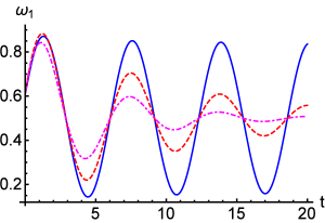
Figure 1: (Color online) The variation of the tomogram with time ($t$) for single spin-$\frac{1}{2}$ atomic coherent state in the presence of QND noise with bath parameters $\gamma_{0}=0.1,\,\omega_{c}=100,$ squeezing parameters $r=0,\,a=0,$ and $\omega=1.0$ and $\alpha=\frac{\pi}{2},\,\beta=\frac{\pi}{3},\,\widetilde{\beta}=\frac{\pi}{3},\,\widetilde{\gamma}=\frac{\pi}{4},$ in the units of $\hbar=k_{B}=1$. The smooth (blue) line, dashed (red) line and dot-dashed (magenta) line correspond to the tomogram with time for different temperatures $T=0,\,1$ and $2$, respectively.

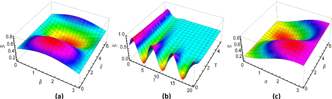
Figure 2: (Color online) The dependence of the tomogram on various parameters is depicted for single spin-$\frac{1}{2}$ atomic coherent state in the presence of QND noise with bath parameters $\gamma_{0}=0.1,\,\omega_{c}=100,$ squeezing parameter $a=0,$ and $\omega=1.0$ in the units of $\hbar=k_{B}=1$. In (a) the tomogram is shown as a function of $\widetilde{\beta}$ and $\widetilde{\gamma}$ with $\alpha=\frac{\pi}{2},\,\beta=\frac{\pi}{3},$ and $r=t=T=1$; while (b) exhibits the variation of the tomogram with time and temperature for $r=0$ and $\alpha=\frac{\pi}{2},\,\beta=\frac{\pi}{3},\,\widetilde{\beta}=\frac{\pi}{3},\,\widetilde{\gamma}=\frac{\pi}{4}$. Finally, the last plot (c) shows the dependence of the tomogram on the atomic coherent state parameters $\alpha$ and $\beta$ with $\widetilde{\beta}=\frac{\pi}{3},\,\widetilde{\gamma}=\frac{\pi}{4}$ at time $t=1$ for bath squeezing parameter $r=1$ at $T=1$.

II.2 Dissipative SGAD channel

Master equation for the dissipative evolution of a given state in the squeezed generalized amplitude damping (SGAD) channel is given by SGAD

$$\begin{array}[]{lcl}\frac{d}{dt}\rho^{s}\left(t\right)&=&-\frac{i\omega}{2}\left[\sigma_{z},\rho^{s}\left(t\right)\right]+\gamma_{0}\left(N+1\right)\left\{\sigma_{-}\rho^{s}\left(t\right)\sigma_{+}-\frac{1}{2}\sigma_{+}\sigma_{-}\rho^{s}\left(t\right)-\frac{1}{2}\rho^{s}\left(t\right)\sigma_{+}\sigma_{-}\right\}\\ &+&\left\{\sigma_{+}\rho^{s}\left(t\right)\sigma_{-}-\frac{1}{2}\sigma_{-}\sigma_{+}\rho^{s}\left(t\right)-\frac{1}{2}\rho^{s}\left(t\right)\sigma_{-}\sigma_{+}\right\}\gamma_{0}N-\gamma_{0}M\sigma_{+}\rho^{s}\left(t\right)\sigma_{+}-\gamma_{0}M^{*}\sigma_{-}\rho^{s}\left(0\right)\sigma_{-}.\end{array}$$ (16)

The density matrix for a quantum state under a dissipative SGAD channel at time $t$ can be obtained, from the above equation, as

$$\begin{array}[]{lcl}\rho^{s}\left(t\right)&=&\frac{1}{4}\rho^{s}\left(0\right)f_{+}+\frac{1}{4}\sigma_{z}\rho^{s}\left(0\right)\sigma_{z}f_{-}-\frac{1}{4}\rho^{s}\left(0\right)\sigma_{z}g_{-}-\frac{1}{4}\sigma_{z}\rho^{s}\left(0\right)g_{+}-\gamma_{0}\frac{\sinh\left(\alpha^{\prime}t\right)}{\alpha^{\prime}}e^{-\frac{\gamma^{\beta}t}{2}}\\ &\times&\left\{M\sigma_{+}\rho^{s}\left(0\right)\sigma_{+}+M^{*}\sigma_{-}\rho^{s}\left(0\right)\sigma_{-}\right\}+\left(1-e^{-\gamma^{\beta}t}\right)\left\{\frac{\gamma_{+}}{\gamma^{\beta}}\sigma_{-}\rho^{s}\left(0\right)\sigma_{+}+\frac{\gamma_{-}}{\gamma^{\beta}}\sigma_{+}\rho^{s}\left(0\right)\sigma_{-}\right\},\end{array}$$ (17)

where $f_{\pm}=\left\{1+e^{-\gamma^{\beta}t}\pm 2\cosh\left(\alpha^{\prime}t\right)e^{-\frac{\gamma^{\beta}t}{2}}\right\},$ $g_{\pm}=\left\{\frac{\gamma}{\gamma^{\beta}}\left(1-e^{-\gamma^{\beta}t}\right)\pm\frac{2i\omega}{\alpha^{\prime}}\sinh\left(\alpha^{\prime}t\right)e^{-\frac{\gamma^{\beta}t}{2}}\right\},$ $\gamma_{+}=\gamma_{0}\left(N+1\right)$, $\gamma_{-}=\gamma_{0}N$, $\gamma^{\beta}=\gamma_{+}+\gamma_{-}$, $\gamma=\gamma_{+}-\gamma_{-}=\gamma_{0}$, $\alpha^{\prime}=\sqrt{\gamma_{0}^{2}\left|M\right|^{2}-\omega^{2}}$; and

$$\begin{array}[]{lcl}\sigma_{+}&=&|1\rangle\langle 0|,\,\,\sigma_{-}=|0\rangle\langle 1|,\\ \sigma_{z}&=&\sigma_{+}\sigma_{-}-\sigma_{-}\sigma_{+}\\ &=&|1\rangle\langle 1|-|0\rangle\langle 0|\\ &=&|e\rangle\langle e|-|g\rangle\langle g|.\end{array}$$

Also,

$$\begin{array}[]{lclccc}\sigma_{z}|g\rangle&=&-|g\rangle,&\sigma_{z}|e\rangle&=&|e\rangle;\\ \sigma_{+}|g\rangle&=&|e\rangle,&\sigma_{+}|e\rangle&=&0;\\ \sigma_{-}|g\rangle&=&0,&\sigma_{-}|e\rangle&=&|g\rangle.\end{array}$$

Here, $\gamma_{0}$ is the spontaneous emission rate, $M=-\frac{1}{2}\left\{2N_{th}+1\right\}\exp\left(i\phi\right)\sinh\left(2r\right)$, and $N=N_{th}\left\{\cosh^{2}\left(r\right)+\sinh^{2}\left(r\right)\right\}+\sinh^{2}\left(r\right),$ where $N_{th}=1/\left\{\exp\left(\hbar\omega/k_{B}T\right)-1\right\}$ being the Planck distribution, and $r$ and the bath squeezing angle ($\phi$) are the bath squeezing parameters. The initial state, as for the tomogram of a quantum state under QND evolution, is the atomic coherent state given in Eq. (2). Using Eq. (17), the density matrix can be written as

$$\rho^{s}\left(t\right)=\left[\begin{array}[]{cc}\langle\frac{1}{2}|\rho^{s}\left(t\right)|\frac{1}{2}\rangle&\langle\frac{1}{2}|\rho^{s}\left(t\right)|-\frac{1}{2}\rangle\\ \langle-\frac{1}{2}|\rho^{s}\left(t\right)|\frac{1}{2}\rangle&\langle-\frac{1}{2}|\rho^{s}\left(t\right)|-\frac{1}{2}\rangle\end{array}\right],$$ (18)

where the various terms are

$$\begin{array}[]{lcl}\langle\frac{1}{2}|\rho^{s}\left(t\right)|\frac{1}{2}\rangle&=&\sin^{2}\left(\frac{\alpha}{2}\right)e^{-\gamma^{\beta}t}+\frac{\gamma_{-}}{\gamma^{\beta}}\left(1-e^{-\gamma^{\beta}t}\right),\\ \langle\frac{1}{2}|\rho^{s}\left(t\right)|-\frac{1}{2}\rangle&=&\frac{1}{2}\sin\alpha\left[\left\{\cosh\left(\alpha^{\prime}t\right)-\frac{i\omega}{\alpha^{\prime}}\sinh\left(\alpha^{\prime}t\right)\right\}e^{-i\beta}-\frac{\gamma_{0}M}{\alpha^{\prime}}\sinh\left(\alpha^{\prime}t\right)e^{i\beta}\right]e^{-\frac{\gamma^{\beta}t}{2}},\\ \langle-\frac{1}{2}|\rho^{s}\left(t\right)|\frac{1}{2}\rangle&=&\frac{1}{2}\sin\alpha\left[\left\{\cosh\left(\alpha^{\prime}t\right)+\frac{i\omega}{\alpha^{\prime}}\sinh\left(\alpha^{\prime}t\right)\right\}e^{i\beta}-\frac{\gamma_{0}M^{*}}{\alpha^{\prime}}\sinh\left(\alpha^{\prime}t\right)e^{-i\beta}\right]e^{-\frac{\gamma^{\beta}t}{2}},\\ \langle-\frac{1}{2}|\rho^{s}\left(t\right)|-\frac{1}{2}\rangle&=&\cos^{2}\left(\frac{\alpha}{2}\right)e^{-\gamma^{\beta}t}+\frac{\gamma_{+}}{\gamma^{\beta}}\left(1-e^{-\gamma^{\beta}t}\right),\end{array}$$

and the density matrix can be seen to be normalized as $\stackrel{{\scriptstyle[}}{{m}}=-1/2]{1/2}{\sum}\langle m|\rho^{s}\left(t\right)|m\rangle=1.$

The tomogram of a state evolving in a dissipative SGAD channel, in analogy to the QND case, can be obtained by expanding the density matrix in the basis of the Wigner-Dicke states, as in Eq. (7). Using Eq. (9), the first two relations of Eq. (13) and Eq. (18), the first component of the tomogram is

$$\begin{array}[]{lcl}\omega\left(\frac{1}{2},\widetilde{\alpha},\widetilde{\beta},\widetilde{\gamma}\right)\equiv\omega_{1}&=&\sin^{2}\left(\frac{\widetilde{\beta}}{2}\right)\left\{\cos^{2}\left(\frac{\alpha}{2}\right)e^{-\gamma^{\beta}t}+\frac{\gamma_{+}}{\gamma^{\beta}}\left(1-e^{-\gamma^{\beta}t}\right)\right\}+\cos^{2}\left(\frac{\widetilde{\beta}}{2}\right)\left\{\sin^{2}\left(\frac{\alpha}{2}\right)e^{-\gamma^{\beta}t}+\frac{\gamma_{-}}{\gamma^{\beta}}\left(1-e^{-\gamma^{\beta}t}\right)\right\}\\ &-&\frac{1}{2}\sin\widetilde{\beta}\left\{e^{-i\widetilde{\gamma}}\left[\frac{1}{2}\sin\alpha e^{-i\beta}e^{-\frac{\gamma^{\beta}t}{2}}\left\{\cosh\left(\alpha^{\prime}t\right)-\frac{i\omega}{\alpha^{\prime}}\sinh\left(\alpha^{\prime}t\right)\right\}-\frac{\gamma_{0}M}{2\alpha^{\prime}}\sin\alpha\sinh\left(\alpha^{\prime}t\right)e^{i\beta}e^{-\frac{\gamma^{\beta}t}{2}}\right]\right.\\ &+&\left.{\rm c.c.}\right\}.\end{array}$$ (19)

Again, we can check the validity of the analytic expression of the tomogram in the absence of open system effects, i.e., by considering $\gamma_{0}=\gamma=0$, $\gamma_{+}=\gamma_{-}=0=\gamma^{\beta}$, which leads to $\alpha^{\prime}=i\omega$, we have

$$\begin{array}[]{lcl}\omega\left(\frac{1}{2},\widetilde{\alpha},\widetilde{\beta},\widetilde{\gamma}\right)&=&\cos^{2}\left(\frac{\widetilde{\beta}}{2}\right)-\cos\widetilde{\beta}\cos^{2}\left(\frac{\alpha}{2}\right)-\frac{1}{2}\sin\widetilde{\beta}\sin\alpha\cos\left(\omega t+\beta+\widetilde{\gamma}\right),\end{array}$$ (20)

which is identical to the QND case, i.e., Eq. (14), with $\gamma\left(t\right)=0$. Similarly, using Eq. (9), the last two relations of Eq. (13), and Eq. (18), we obtain the second component as

$$\begin{array}[]{lcl}\omega\left(-\frac{1}{2},\widetilde{\alpha},\widetilde{\beta},\widetilde{\gamma}\right)\equiv\omega_{2}&=&\cos^{2}\left(\frac{\widetilde{\beta}}{2}\right)\left\{\cos^{2}\left(\frac{\alpha}{2}\right)e^{-\gamma^{\beta}t}+\frac{\gamma_{+}}{\gamma^{\beta}}\left(1-e^{-\gamma^{\beta}t}\right)\right\}+\sin^{2}\left(\frac{\widetilde{\beta}}{2}\right)\left\{\sin^{2}\left(\frac{\alpha}{2}\right)e^{-\gamma^{\beta}t}+\frac{\gamma_{-}}{\gamma^{\beta}}\left(1-e^{-\gamma^{\beta}t}\right)\right\}\\ &+&\frac{1}{2}\sin\widetilde{\beta}\left\{e^{-i\widetilde{\gamma}}\left[\frac{1}{2}\sin\alpha e^{-i\beta}e^{-\frac{\gamma^{\beta}t}{2}}\left\{\cosh\left(\alpha^{\prime}t\right)-\frac{i\omega}{\alpha^{\prime}}\sinh\left(\alpha^{\prime}t\right)\right\}-\frac{\gamma_{0}M}{2\alpha^{\prime}}\sin\alpha\sinh\left(\alpha^{\prime}t\right)e^{i\beta}e^{-\frac{\gamma^{\beta}t}{2}}\right]\right.\\ &+&\left.{\rm c.c.}\right\}.\end{array}$$ (21)

Similar to the first tomogram of the dissipative SGAD channel, we can check the solution in the absence of the open system effects which leads to $\alpha^{\prime}=i\omega$. This can be seen to be the same as the corresponding QND case, i.e., Eq. (15), with $\gamma\left(t\right)=0$

$$\begin{array}[]{lcl}\omega\left(-\frac{1}{2},\widetilde{\alpha},\widetilde{\beta},\widetilde{\gamma}\right)&=&\cos^{2}\left(\frac{\widetilde{\beta}}{2}\right)-\cos\widetilde{\beta}\sin^{2}\left(\frac{\alpha}{2}\right)+\frac{1}{2}\sin\widetilde{\beta}\sin\alpha\cos\left(\omega t+\beta+\widetilde{\gamma}\right).\end{array}$$ (22)

We can also check the validity of the tomogram as in the QND case by $\sum\omega_{i}=\omega_{1}+\omega_{2}=1.$ Hence, as before, one component of the tomogram would be enough to recover all the information. This is why, in the plots, we only show the first component of the tomogram. The other component can be easily obtained from it.

The variation of tomogram with different parameters is shown in Figs. 3 and 4. Fig. 3 exhibits the randomization of the tomogram with increase in temperature. This fact can be observed in the smooth (blue) and dashed (red) lines. However, an interesting behavior is observed here with respect to bath squeezing. It can be seen that it takes relatively longer to randomize the tomogram in presence of squeezing than in its absence, temperature remaining same, as illustrated by a comparison between the dot-dashed (magenta) and dashed (red) line. This fact, in turn, establishes that squeezing is a useful quantum resource. This behavior is further elaborated in Fig. 4, where the effect of bath squeezing can be observed and is consistent with the quadrature behavior of squeezing. This beneficial effect of squeezing is not observed for evolution under QND channel. From the present analysis, it could be envisaged that a tomographic connection could be established between the state, under consideration and the generic open system interaction evolving it.

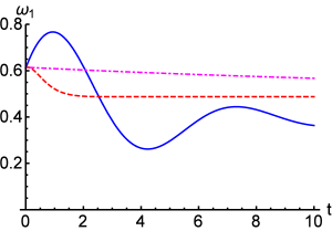
Figure 3: (Color online) The tomogram varying with time ($t$) is shown for a single spin-$\frac{1}{2}$ atomic coherent state in the presence of the SGAD noise for bath squeezing angle $\phi=\pi$ in the units of $\hbar=k_{B}=1$, with $\omega=1.0,\,\gamma_{0}=0.25,$ and $\alpha=\frac{\pi}{2},\,\beta=\frac{\pi}{3},\,\widetilde{\beta}=\frac{\pi}{3},\,\widetilde{\gamma}=\frac{\pi}{4}$. The smooth (blue) line, dashed (red) line and dot-dashed (magenta) line correspond to the tomogram with time for different temperatures and squeezing parameters $T=1,\,10$ and $10$, and $r=0,\,0$ and $1$, respectively.

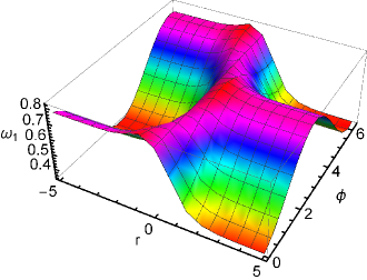
Figure 4: (Color online) The tomogram for single spin-$\frac{1}{2}$ atomic coherent state in the presence of SGAD noise is shown as a function of squeezing parameters $r$ and $\phi$ with $\alpha=\frac{\pi}{2},\,\beta=\frac{\pi}{3},\,\widetilde{\beta}=\frac{\pi}{3},\,\widetilde{\gamma}=\frac{\pi}{4},$ and $\omega=1.0,\,\gamma_{0}=0.25,$ in the units of $\hbar=k_{B}=1$ for $T=1$ at time $t=1$.

III Tomogram of two spin-$\frac{1}{2}$ (qubit) states

Various two-qubit tomography schemes have been proposed in the recent past Manko-1/2 ; Manko-2spin ; adam-2qubit-tom ; comment12-ref1 ; comment12-ref2 . Specifically, the tomogram for two spin-$\frac{1}{2}$ (qubit) states can be obtained using the star product scheme Manko-1/2 ; Manko-2spin . In comment12-ref1 , two-qubit states were analyzed from the perspective of tomographic causal analysis, while in comment12-ref2 , an interesting connection between tomographic construction of two-qubit states to aspects of quantum correlations such as discord and measurement induced disturbance was developed.

For a two qubit state $\rho$ one can obtain the tomogram as

$$\omega\left(m_{1},m_{2}\right)={\rm Tr}\left[\rho\left\{Q_{1}\left(m_{1}\right)\otimes Q_{2}\left(m_{2}\right)\right\}\right],$$ (23)

where $Q_{i}\left(m_{i}\right)=U_{i}^{\dagger}\left|m_{i}\right\rangle\left\langle m_{i}\right|U_{i},$ and $m_{i}=\pm\frac{1}{2},$ while the unitary matrices $U_{i}$ are

$$U_{i}=\left[\begin{array}[]{cc}\cos\frac{\widetilde{\beta}_{i}}{2}\exp\left\{\frac{i\left(\widetilde{\alpha}_{i}+\widetilde{\gamma}_{i}\right)}{2}\right\}&\sin\frac{\widetilde{\beta}_{i}}{2}\exp\left\{\frac{i\left(\widetilde{\alpha}_{i}-\widetilde{\gamma}_{i}\right)}{2}\right\}\\ -\sin\frac{\widetilde{\beta}_{i}}{2}\exp\left\{-\frac{i\left(\widetilde{\alpha}_{i}-\widetilde{\gamma}_{i}\right)}{2}\right\}&\cos\frac{\widetilde{\beta}_{i}}{2}\exp\left\{-\frac{i\left(\widetilde{\alpha}_{i}+\widetilde{\gamma}_{i}\right)}{2}\right\}\end{array}\right]$$

for $i\in\left\{1,2\right\}.$ Hence, the tomogram of the two qubit state can be written as the diagonal elements of $\widetilde{\rho},$ where $\widetilde{\rho}=\left(U_{1}\otimes U_{2}\right)\rho\left(U_{1}\otimes U_{2}\right)^{\dagger}.$

III.1 Tomogram of two qubits under dissipative evolution in a vacuum bath

Now, we construct the tomogram of a two qubit state in a vacuum bath under dissipative evolution, as discussed in Ref. squ-ther-bath . The initial state of the system is considered with one qubit in the excited state $\left|e_{1}\right\rangle$ and the other in the ground state $\left|g_{2}\right\rangle$, i.e., $\left|e_{1}\right\rangle\left|g_{2}\right\rangle$. The reduced density matrix of the system of interest, here the two qubits, is

$$\begin{array}[]{lcl}\rho\left(t\right)&=&\left[\begin{array}[]{cccc}\rho_{ee}\left(t\right)&\rho_{es}\left(t\right)&\rho_{ea}\left(t\right)&\rho_{eg}\left(t\right)\\ \rho_{es}^{*}\left(t\right)&\rho_{ss}\left(t\right)&\rho_{sa}\left(t\right)&\rho_{sg}\left(t\right)\\ \rho_{ea}^{*}\left(t\right)&\rho_{sa}^{*}\left(t\right)&\rho_{aa}\left(t\right)&\rho_{ag}\left(t\right)\\ \rho_{eg}^{*}\left(t\right)&\rho_{sg}^{*}\left(t\right)&\rho_{ag}^{*}\left(t\right)&\rho_{gg}\left(t\right)\end{array}\right],\end{array}$$ (24)

where the analytic form of all the elements of the density matrix is given in Appendix 1.

The tomogram can be thought of as a tomographic-probability vector $\omega=\left[\omega_{1},\omega_{2},\omega_{3},\omega_{4}\right]^{T}$ (here $T$ corresponds to transpose of the vector), where each component can be expressed analytically as

$$\begin{array}[]{lcl}\omega_{1}\left(t\right)&=&\frac{1}{4}\left[4\rho_{ee}\cos^{2}\frac{\widetilde{\beta}_{1}}{2}\cos^{2}\frac{\widetilde{\beta}_{2}}{2}+4\rho_{gg}\sin^{2}\frac{\widetilde{\beta}_{1}}{2}\sin^{2}\frac{\widetilde{\beta}_{2}}{2}\right.+\left(\rho_{aa}+\rho_{ss}\right)\left(1-\cos\widetilde{\beta}_{1}\cos\widetilde{\beta}_{2}\right)\\ &-&\left(\rho_{aa}-\rho_{ss}\right)\sin\widetilde{\beta}_{1}\sin\widetilde{\beta}_{2}\cos\left(\widetilde{\gamma}_{1}-\widetilde{\gamma}_{2}\right)+\left\{\rho_{sa}\left(\cos\widetilde{\beta}_{1}-\cos\widetilde{\beta}_{2}-i\sin\widetilde{\beta}_{1}\sin\widetilde{\beta}_{2}\right.\sin\left(\widetilde{\gamma}_{1}-\widetilde{\gamma}_{2}\right)\right)\\ &+&\sqrt{2}\left[\left(\left(-\rho_{ea}+\rho_{es}\right)\cos^{2}\frac{\widetilde{\beta}_{2}}{2}+\left(\rho_{ag}+\rho_{sg}\right)\sin^{2}\frac{\widetilde{\beta}_{2}}{2}\right)\right.\sin\widetilde{\beta}_{1}\exp\left(i\widetilde{\gamma}_{1}\right)+\sin\widetilde{\beta}_{2}\exp\left(i\widetilde{\gamma}_{2}\right)\\ &\times&\left.\left(\left(\rho_{ea}+\rho_{es}\right)\cos^{2}\frac{\widetilde{\beta}_{1}}{2}-\left(\rho_{ag}-\rho_{sg}\right)\sin^{2}\frac{\widetilde{\beta}_{1}}{2}\right)\right]+\left.\left.\exp\left(i\widetilde{\gamma}_{1}+i\widetilde{\gamma}_{2}\right)\rho_{eg}\sin\widetilde{\beta}_{1}\sin\widetilde{\beta}_{2}+{\rm c.c.}\right\}\right],\end{array}$$ (25)

$$\begin{array}[]{lcl}\omega_{2}\left(t\right)&=&\frac{1}{4}\left[4\rho_{ee}\cos^{2}\frac{\widetilde{\beta}_{1}}{2}\sin^{2}\frac{\widetilde{\beta}_{2}}{2}+4\rho_{gg}\sin^{2}\frac{\widetilde{\beta}_{1}}{2}\cos^{2}\frac{\widetilde{\beta}_{2}}{2}\right.+\left(\rho_{aa}+\rho_{ss}\right)\left(1+\cos\widetilde{\beta}_{1}\cos\widetilde{\beta}_{2}\right)\\ &+&\left(\rho_{aa}-\rho_{ss}\right)\sin\widetilde{\beta}_{1}\sin\widetilde{\beta}_{2}\cos\left(\widetilde{\gamma}_{1}-\widetilde{\gamma}_{2}\right)+\left\{\rho_{sa}\left(\cos\widetilde{\beta}_{1}+\cos\widetilde{\beta}_{2}+i\sin\widetilde{\beta}_{1}\sin\widetilde{\beta}_{2}\right.\sin\left(\widetilde{\gamma}_{1}-\widetilde{\gamma}_{2}\right)\right)\\ &+&\sqrt{2}\left[\left(\left(\rho_{ag}+\rho_{sg}\right)\cos^{2}\frac{\widetilde{\beta}_{2}}{2}-\left(\rho_{ea}-\rho_{es}\right)\sin^{2}\frac{\widetilde{\beta}_{2}}{2}\right)\sin\widetilde{\beta}_{1}\exp\left(i\widetilde{\gamma}_{1}\right)\right.\\ &+&\sin\widetilde{\beta}_{2}\exp\left(i\widetilde{\gamma}_{2}\right)\left.\left(-\left(\rho_{ea}+\rho_{es}\right)\cos^{2}\frac{\widetilde{\beta}_{1}}{2}+\left(\rho_{ag}-\rho_{sg}\right)\sin^{2}\frac{\widetilde{\beta}_{1}}{2}\right)\right]-\left.\left.\exp\left(i\widetilde{\gamma}_{1}+i\widetilde{\gamma}_{2}\right)\rho_{eg}\sin\widetilde{\beta}_{1}\sin\widetilde{\beta}_{2}+{\rm c.c.}\right\}\right],\end{array}$$ (26)

$$\begin{array}[]{lcl}\omega_{3}\left(t\right)&=&\frac{1}{4}\left[4\rho_{ee}\sin^{2}\frac{\widetilde{\beta}_{1}}{2}\cos^{2}\frac{\widetilde{\beta}_{2}}{2}+4\rho_{gg}\cos^{2}\frac{\widetilde{\beta}_{1}}{2}\sin^{2}\frac{\widetilde{\beta}_{2}}{2}\right.+\left(\rho_{aa}+\rho_{ss}\right)\left(1+\cos\widetilde{\beta}_{1}\cos\widetilde{\beta}_{2}\right)\\ &+&\left(\rho_{aa}-\rho_{ss}\right)\sin\widetilde{\beta}_{1}\sin\widetilde{\beta}_{2}\cos\left(\widetilde{\gamma}_{1}-\widetilde{\gamma}_{2}\right)+\left\{-\rho_{sa}\left(\cos\widetilde{\beta}_{1}+\cos\widetilde{\beta}_{2}-i\sin\widetilde{\beta}_{1}\sin\widetilde{\beta}_{2}\right.\sin\left(\widetilde{\gamma}_{1}-\widetilde{\gamma}_{2}\right)\right)\\ &+&\sqrt{2}\left[\left(-\left(\rho_{ag}+\rho_{sg}\right)\sin^{2}\frac{\widetilde{\beta}_{2}}{2}+\left(\rho_{ea}-\rho_{es}\right)\cos^{2}\frac{\widetilde{\beta}_{2}}{2}\right)\sin\widetilde{\beta}_{1}\exp\left(i\widetilde{\gamma}_{1}\right)\right.\\ &+&\sin\widetilde{\beta}_{2}\exp\left(i\widetilde{\gamma}_{2}\right)\left.\left(\left(\rho_{ea}+\rho_{es}\right)\sin^{2}\frac{\widetilde{\beta}_{1}}{2}-\left(\rho_{ag}-\rho_{sg}\right)\cos^{2}\frac{\widetilde{\beta}_{1}}{2}\right)\right]-\left.\left.\exp\left(i\widetilde{\gamma}_{1}+i\widetilde{\gamma}_{2}\right)\rho_{eg}\sin\widetilde{\beta}_{1}\sin\widetilde{\beta}_{2}+{\rm c.c.}\right\}\right],\end{array}$$ (27)

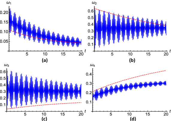
Figure 5: (Color online) Various components of the tomogram changing with time are shown in (a)-(d) for the two-qubit state, in the presence of vacuum bath, with $\widetilde{\beta}_{1}=\frac{\pi}{3},\,\widetilde{\beta}_{2}=\frac{\pi}{4},\,\widetilde{\gamma}_{1}=\frac{\pi}{3},\,\widetilde{\gamma}_{2}=\frac{\pi}{4}$ and the inter-qubit spacing $r_{12}=0.05$ (2.0) corresponding to smooth blue (red dashed) line.

and

$$\begin{array}[]{lcl}\omega_{4}\left(t\right)&=&\frac{1}{4}\left[4\rho_{ee}\sin^{2}\frac{\widetilde{\beta}_{1}}{2}\sin^{2}\frac{\widetilde{\beta}_{2}}{2}+4\rho_{gg}\cos^{2}\frac{\widetilde{\beta}_{1}}{2}\cos^{2}\frac{\widetilde{\beta}_{2}}{2}\right.+\left(\rho_{aa}+\rho_{ss}\right)\left(1-\cos\widetilde{\beta}_{1}\cos\widetilde{\beta}_{2}\right)\\ &-&\left(\rho_{aa}-\rho_{ss}\right)\sin\widetilde{\beta}_{1}\sin\widetilde{\beta}_{2}\cos\left(\widetilde{\gamma}_{1}-\widetilde{\gamma}_{2}\right)+\left\{-\rho_{sa}\left(\cos\widetilde{\beta}_{1}-\cos\widetilde{\beta}_{2}+i\sin\widetilde{\beta}_{1}\sin\widetilde{\beta}_{2}\right.\sin\left(\widetilde{\gamma}_{1}-\widetilde{\gamma}_{2}\right)\right)\\ &+&\sqrt{2}\left[\left(-\left(\rho_{ag}+\rho_{sg}\right)\cos^{2}\frac{\widetilde{\beta}_{2}}{2}+\left(\rho_{ea}-\rho_{es}\right)\sin^{2}\frac{\widetilde{\beta}_{2}}{2}\right)\sin\widetilde{\beta}_{1}\exp\left(i\widetilde{\gamma}_{1}\right)\right.\\ &+&\sin\widetilde{\beta}_{2}\exp\left(i\widetilde{\gamma}_{2}\right)\left.\left(-\left(\rho_{ea}+\rho_{es}\right)\sin^{2}\frac{\widetilde{\beta}_{1}}{2}+\left(\rho_{ag}-\rho_{sg}\right)\cos^{2}\frac{\widetilde{\beta}_{1}}{2}\right)\right]-\left.\left.\exp\left(i\widetilde{\gamma}_{1}+i\widetilde{\gamma}_{2}\right)\rho_{eg}\sin\widetilde{\beta}_{1}\sin\widetilde{\beta}_{2}+{\rm c.c.}\right\}\right].\end{array}$$ (28)

Here, $\rho_{ij}$ are the elements of the matrix in Eq. (24) and are given in Appendix 1. For simplicity of notations the time dependence in the arguments of matrix elements is omitted. Similar to the tomograms for single spin-$\frac{1}{2}$ states the tomogram obtained here is also free from $\widetilde{\alpha}.$

As in the cases of single qubit tomograms, we can again verify that the tomogram obtained here satisfies the condition $\sum\omega_{i}=\rho_{ee}+\rho_{gg}+\rho_{aa}+\rho_{ss},$ which is the trace of the density matrix given in Eq. (24), and hence equal to one.

For the case of identical qubits considered here, we take the wave-vector and mean frequency to be $k_{0}=\omega_{0}=1$, the spontaneous emission rate $\Gamma_{j}=0.05$ and $\hat{\mu}\cdot\hat{r}_{ij}=0$. Here, $\hat{\mu}$ is the unit vector along the atomic transition dipole moment and $\hat{r}_{ij}$ is the inter-atomic distance. Further, the initial state of the system is taken to be $\rho_{ee}\left(0\right)=\rho_{gg}\left(0\right)=\rho_{es}\left(0\right)=\rho_{ea}\left(0\right)=\rho_{eg}\left(0\right)=\rho_{sg}\left(0\right)=\rho_{ag}\left(0\right)=0$, and $\rho_{ss}\left(0\right)=\rho_{aa}\left(0\right)=\rho_{sa}\left(0\right)=0.5$.

The variation of all four components of the tomogram is shown with different parameters in Figs. 5 and 6. In Fig. 5, large oscillations can be observed for small interqubit spacing, which is consistent with the earlier observations in a plethora of scenario our-qd-paper ; squ-ther-bath ; GP . Fig. 6 further demonstrates similar behavior for small interqubit spacing. For small interqubit spacing the ambient environment opens up a channel between the qubits resulting in enhancement of oscillations.

IV Tomogram of single spin-1 state

The tomograms for finite spin states have been considered, among others, in Refs. manko-spin-tom ; spin-j-tom ; manko-spin ; comment6-ref1 . In continuation with the theme of this work, we take up an arbitrary spin-1 state

$$\begin{array}[]{lcl}\psi^{\left(1\right)}&=&N\left[\begin{array}[]{c}a\\ b\\ c\end{array}\right]\end{array},$$ (29)

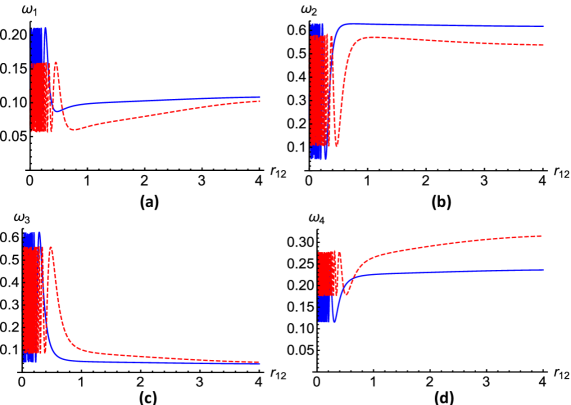
Figure 6: (Color online) (a)-(d) depict the tomogram for the two qubit state, interacting with a vacuum bath, as a function of the inter-qubit spacing at $t=1$ (smooth blue line), and $t=5$ (red dashed line). For all the plots $\widetilde{\beta}_{1}=\frac{\pi}{3},\,\widetilde{\beta}_{2}=\frac{\pi}{4},\,\widetilde{\gamma}_{1}=\frac{\pi}{3},\,\widetilde{\gamma}_{2}=\frac{\pi}{4}$.

where $N=\frac{1}{\sqrt{\left|a\right|^{2}+\left|b\right|^{2}+\left|c\right|^{2}}}$ is the normalization factor. The corresponding density matrix is

$$\begin{array}[]{lcl}\rho^{\left(1\right)}&=&\left|N\right|^{2}\left[\begin{array}[]{ccc}\left|a\right|^{2}&ab^{*}&ac^{*}\\ a^{*}b&\left|b\right|^{2}&bc^{*}\\ a^{*}c&b^{*}c&\left|c\right|^{2}\end{array}\right]\end{array}.$$ (30)

Here, we restrict ourselves to obtaining the tomogram for the state (30), without considering open system effects. Using Eqs. (9)-(11), all the Wigner $D$-functions for the tomogram can be calculated as before. Using Eqs. (9) and (30), $\omega\left(1,\widetilde{\alpha},\widetilde{\beta},\widetilde{\gamma}\right)$ can be written as

$$\begin{array}[]{lcl}\omega\left(1,\widetilde{\alpha},\widetilde{\beta},\widetilde{\gamma}\right)\equiv\omega_{1}&=&\left|N\right|^{2}\left[\left\{\frac{\left|a\right|^{2}}{4}\left(1+\cos\widetilde{\beta}\right)^{2}+\frac{\left|b\right|^{2}}{2}\sin^{2}\widetilde{\beta}+\frac{\left|c\right|^{2}}{4}\left(1-\cos\widetilde{\beta}\right)^{2}\right\}\right.\\ &+&\left.\left\{\left(-\frac{ab^{*}e^{i\widetilde{\gamma}}}{2\sqrt{2}}\right)\sin\widetilde{\beta}\left(1+\cos\widetilde{\beta}\right)+\frac{ac^{*}e^{2i\widetilde{\gamma}}}{4}\sin^{2}\widetilde{\beta}-\frac{bc^{*}e^{i\widetilde{\gamma}}}{2\sqrt{2}}\sin\widetilde{\beta}\left(1-\cos\widetilde{\beta}\right)+{\rm c.c.}\right\}\right].\end{array}$$ (31)

Similarly, $\omega\left(0,\widetilde{\alpha},\widetilde{\beta},\widetilde{\gamma}\right)$ can be obtained as

$$\begin{array}[]{lcl}\omega\left(0,\widetilde{\alpha},\widetilde{\beta},\widetilde{\gamma}\right)&\equiv\omega_{0}=&\left|N\right|^{2}\left[\left\{\frac{\left|a\right|^{2}}{2}\sin^{2}\widetilde{\beta}+\left|b\right|^{2}\cos^{2}\widetilde{\beta}+\frac{\left|c\right|^{2}}{2}\sin^{2}\widetilde{\beta}\right\}\right.\\ &+&\left.\left\{\frac{ab^{*}e^{i\widetilde{\gamma}}}{2\sqrt{2}}\sin 2\widetilde{\beta}-\frac{ac^{*}e^{2i\widetilde{\gamma}}}{2}\sin^{2}\widetilde{\beta}-\frac{bc^{*}e^{i\widetilde{\gamma}}}{2\sqrt{2}}\sin 2\widetilde{\beta}+{\rm c.c.}\right\}\right].\end{array}$$ (32)

Also, $\omega\left(-1,\widetilde{\alpha},\widetilde{\beta},\widetilde{\gamma}\right)$ is

$$\begin{array}[]{lcl}\omega\left(-1,\widetilde{\alpha},\widetilde{\beta},\widetilde{\gamma}\right)\equiv\omega_{-1}&=&\left|N\right|^{2}\left[\left\{\frac{\left|a\right|^{2}}{4}\left(1-\cos\widetilde{\beta}\right)^{2}+\frac{\left|b\right|^{2}}{2}\sin^{2}\widetilde{\beta}+\frac{\left|c\right|^{2}}{4}\left(1+\cos\widetilde{\beta}\right)^{2}\right\}\right.\\ &+&\left.\left\{\frac{ab^{*}e^{i\widetilde{\gamma}}}{2\sqrt{2}}\sin\widetilde{\beta}\left(1-\cos\widetilde{\beta}\right)+\frac{ac^{*}e^{2i\widetilde{\gamma}}}{4}\sin^{2}\widetilde{\beta}+\frac{bc^{*}e^{i\widetilde{\gamma}}}{2\sqrt{2}}\sin\widetilde{\beta}\left(1+\cos\widetilde{\beta}\right)+{\rm c.c.}\right\}\right].\end{array}$$ (33)

Interestingly, the tomogram obtained for a general spin-1 quantum state is also free from $\widetilde{\alpha}$ as for spin-$\frac{1}{2}$ cases discussed above. Further, it can be checked here that the tomogram satisfies the condition $\omega_{1}+\omega_{0}+\begin{array}[]{lcl}\omega_{-1}&=&1.\end{array}$ For $a=1,b=0=c$, the tomogram, obtained here, is seen to be consistent with the results reported earlier manko-spin ,

$$\begin{array}[]{lcl}\omega\left(1,\widetilde{\alpha},\widetilde{\beta},\widetilde{\gamma}\right)&=&\frac{\left(1+\cos\widetilde{\beta}\right)^{2}}{4},\\ \omega\left(0,\widetilde{\alpha},\widetilde{\beta},\widetilde{\gamma}\right)&=&\frac{\left(1-\cos^{2}\widetilde{\beta}\right)}{2},\\ \omega\left(-1,\widetilde{\alpha},\widetilde{\beta},\widetilde{\gamma}\right)&=&\frac{\left(1-\cos\widetilde{\beta}\right)^{2}}{4}.\end{array}$$ (34)

The variation of all three components of the tomogram with Euler angles is given in Fig. 7. The peaks in one component have corresponding valleys in other components of the tomogram, which are manifestations of normalization of the tomogram to one.

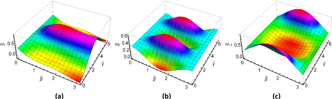
Figure 7: (Color online) The dependence of all three components of tomogram for single spin-1 state with Euler angles for $a=b=c=\frac{1}{\sqrt{3}}$.

V Tomogram of a finite dimensional state

In this section, we discuss tomography of finite dimensional states. The tomogram of a finite dimensional state can be defined as fss-tom

$$\omega\left(m,t,q\right)=\stackrel{{\scriptstyle[}}{{\chi}}=0]{d-1}{\sum}W\left(tm-q\chi,qm+t\chi\right),$$ (35)

where $W\left(\chi,m\right)$ is the discrete Wigner function with integers $t$ and $q$, depicting complementarity between number $m$ (denoting angular momentum) and phase $\chi$ of finite dimensional states. Here, the discrete Wigner function is expressed as

$$W\left(\chi,m\right)=\frac{1}{d}\stackrel{{\scriptstyle[}}{{\Theta}}=0]{d-1}{\sum}\exp\left(\frac{4\pi i}{d}m\Theta\right)\left\langle\chi-\Theta\right|\rho\left|\chi+\Theta\right\rangle.$$ (36)

It would be apt here to mention that the phase states $\left|\chi\right\rangle$ are periodic, such that $\left|\chi+d\right\rangle=\left|\chi\right\rangle$. A general $d$ dimensional density matrix can be written in Weyl operator basis as gen-bloch-vector

$$\rho=\frac{1}{d}\mathbb{I}+\stackrel{{\scriptstyle[}}{{n}},m=0]{d-1}{\sum}b_{nm}U_{nm}$$ (37)

with $b_{00}=0$ and $U_{nm}=\stackrel{{\scriptstyle[}}{{\alpha}}=0]{d-1}{\sum}\exp\left(\frac{2\pi i}{d}{\alpha}n\right)\left|\alpha\right\rangle\left\langle\alpha+m\right|$. We make use of the periodicity of phase states in computations involving $U_{nm}$.

Up to now the treatment is applicable to any generic finite dimensional system. Here, for concreteness, we concentrate on an important finite dimensional system, viz. a qutrit with $d=3$. We study the effect of spontaneous emission (SE) channel noisy-qutrit on the qutrit. SE is a dissipative process which can be modeled by the following Kraus operators

$$\begin{array}[]{lcl}K_{0}&=&\left[\begin{array}[]{ccc}1&0&0\\ 0&e^{-\frac{\eta_{1}t}{2}}&0\\ 0&0&e^{-\frac{\eta_{2}t}{2}}\end{array}\right],\end{array}$$

$$\begin{array}[]{lcl}K_{1}&=&\left[\begin{array}[]{ccc}0&\sqrt{1-e^{-\eta_{1}t}}&0\\ 0&0&0\\ 0&0&0\end{array}\right],\end{array}$$

$$\begin{array}[]{lcl}K_{2}&=&\left[\begin{array}[]{ccc}0&0&\sqrt{1-e^{-\eta_{2}t}}\\ 0&0&0\\ 0&0&0\end{array}\right],\end{array}$$ (38)

where $\eta_{1}$ and $\eta_{2}$ are two Einstein coefficients which control the population of the excited states. Thus, we can write the density matrix of an arbitrary three dimensional state at time $t$ evolving under the spontaneous emission channel as

$$\rho\left(t\right)=\stackrel{{\scriptstyle[}}{{j}},k=0]{2}{\sum}A_{jk}\left(t\right)\left|j\right\rangle\left\langle k\right|=\stackrel{{\scriptstyle[}}{{i}}=0]{2}{\sum}K_{i}\rho\left(0\right)K_{i}^{\dagger}.$$ (39)

Using this we can obtain

$$W\left(\chi,m,t\right)=\frac{1}{3}\stackrel{{\scriptstyle[}}{{\Theta}}=0]{2}{\sum}A_{\chi-\Theta,\chi+\Theta}\left(t\right)\exp\left(\frac{4\pi i}{3}m\Theta\right).$$ (40)

As mentioned above $\chi-\Theta$ and $\chi+\Theta$ are mod $d$ operations. Here, we have considered an initial density matrix given by Eq. (37) with $b_{01}=b_{10}=\frac{1}{4}$ and $b_{12}=b_{21}=\frac{1}{5}$, while the remaining coefficients can be obtained from these values. Hence, the obtained tomogram with $t=0$ and $q=1$ has three components as

$$\begin{array}[]{lcl}\omega\left(0,0,1\right)\equiv\omega_{0}&=&\frac{1}{30}\left[10+7\left(e^{-\frac{\eta_{1}t}{2}}+e^{-\frac{\eta_{2}t}{2}}\right)+e^{-\frac{1}{2}\left(\eta_{1}+\eta_{2}\right)t}\right],\\ \omega\left(1,0,1\right)\equiv\omega_{1}&=&\frac{1}{60}\left[20-\left(e^{-\frac{\eta_{1}t}{2}}+e^{-\frac{\eta_{2}t}{2}}\right)-13e^{-\frac{1}{2}\left(\eta_{1}+\eta_{2}\right)t}\right],\\ \omega\left(2,0,1\right)\equiv\omega_{2}&=&\frac{1}{60}\left[20-13\left(e^{-\frac{\eta_{1}t}{2}}+e^{-\frac{\eta_{2}t}{2}}\right)+11e^{-\frac{1}{2}\left(\eta_{1}+\eta_{2}\right)t}\right].\end{array}$$ (41)

It can be easily seen here that the tomogram obtained is normalized as $\stackrel{{\scriptstyle[}}{{m}}=0]{2}{\sum}\omega_{m}=1$ in Eq. (41).

For specific values of parameters of the spontaneous emission channel, i.e., Einstein coefficients, the evolution of tomogram for the qutrit state is shown in Fig. 8. The tomogram shows that the noisy channel tends to randomize all the components of the tomogram to one-third. We have already noted that once a tomogram is obtained for a finite dimensional system, it is possible to transform it to obtain the Wigner function for the system, and vice verse, but in an experiment we obtain tomograms. A lot of work has been devoted to the study of Wigner functions for finite dimensional systems adam-wig1 ; adam-wig2 ; with-adam ; with-jay . Some efforts have also been made to study tomograms for finite dimensional coherent states with-adam ; with-jay ; manko-fss . However, to the best of our knowledge, no such efforts had yet been made to study evolution of tomograms in noisy environment.

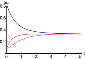
Figure 8: (Color online) The variation of different components of tomogram for a qutrit state with time in the presence of a spontaneous emission channel with Einstein coefficients $\eta_{1}=2$ and $\eta_{2}=4$. The smooth (blue), dashed (red) and dot-dashed (magenta) lines correspond to $\omega_{m}$ with $m=0,\,1,$ and 2, respectively.

VI Optical tomogram for a dissipative harmonic oscillator

In the end, we come to the tomogram of an infinite dimensional system, the harmonic oscillator. This is typical of a plethora of oscillatory and optical systems louis ; perina-book . In Ref. comment13-ref1 , the quantum mechanics of the damped harmonic oscillator was examined, from the perspective of a classical description of quantum mechanics tombesi96 . Use was made of the generating function method, resulting in the avoidance of the need to evaluate the Wigner function as an intermediary step for obtaining the tomogram. Further, in comment13-ref2 the density matrix, state tomogram and Wigner function of a parametric oscillator were studied.

Here, we construct the tomogram of the dissipative harmonic oscillator evolving under a Lindbladian evolution, in a phase sensitive reservoir op-tom-rho . It would be pertinent to mention that tomographic reconstruction of Gaussian states evolving under a Markovian evolution has also been considered in marzolino1 . The dissipative harmonic oscillator can be described by the Hamiltonian

$$H=H_{S}+H_{R}+H_{SR},$$ (42)

where the system Hamiltonian $H_{s}$ of a harmonic oscillator is described as

$$H_{S}=\frac{p^{2}}{2m}+\frac{1}{2}m\omega^{2}x^{2},$$

while the reservoir Hamiltonian $H_{R}$ is given by

$$H_{R}=\sum_{j}\frac{p_{j}^{2}}{2m_{j}}+\frac{1}{2}m_{j}\omega_{j}^{2}x_{j}^{2},$$

with the system-reservoir interaction Hamiltonian $H_{SR}$ as

$$H_{SR}=\sum_{j}c_{j}xx_{j}.$$

Here, the reservoir is modeled as a bath of harmonic oscillators with $c_{j}$ as the coupling constant. The dynamics of the system harmonic oscillator is obtained by tracing over the reservoir degrees of freedom. The optical tomogram from the Wigner function can be obtained using op-tom

$$\begin{array}[]{l}\omega\left(X,\theta\right)=\int W\left(X\cos\theta-p\sin\theta,X\sin\theta+p\cos\theta\right)dp,\end{array}$$ (43)

where $W\left(x,y,t\right)$ is the Wigner function. Similarly, the corresponding Wigner function can also be reconstructed from the tomogram by inverse Radon transformation. The analytic expression of the tomogram for the system, initially in the coherent state $\left|\beta\right\rangle,$ is

$$\begin{array}[]{lcl}\omega(X,\theta,t)&=&\sqrt{\frac{2}{\pi}}\frac{1}{\sqrt{\left(2NM+1\right)-\left(rMe^{-2i\theta}+{\rm c.c.}\right)}}\exp\left(-\frac{2\left(Re[\beta e^{i\theta}]e^{-kt}-X\right)^{2}}{\left(2NM+1\right)-\left(rMe^{-2i\theta}+{\rm c.c.}\right)}\right).\end{array}$$ (44)

Here, $k_{B}$ is the Boltzmann constant and $N=\frac{1}{\exp(\hbar\omega_{k}/k_{B}T)-1}$ is the average thermal photon number of the environment at temperature $T$. Also, $r$ is the bath squeezing parameter, $Re[u]$ denotes the real part of $u$ and $M=1-\exp\left(-2kt\right),$ where $k$ is the dissipation coefficient, analogous to the spontaneous emission term.

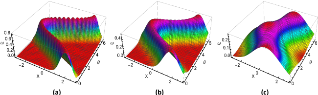
Figure 9: (Color online) The effect of interaction of the optical tomogram with its environment is shown as a function of $X$ and $\theta$ for $N=5,\,r=1$ for the initial coherent state parameter $\beta=2$ at time $t=0,\,1,\,10$, respectively.

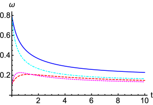
Figure 10: (Color online) The tomogram of a dissipative harmonic oscillator varying with time is shown for the initial coherent state parameter $\beta=2$ and $\theta=\frac{\pi}{3}$. The smooth (blue) and dashed (red) lines correspond to the tomogram for $N=5,\,r=1$ for $X=1$ and 2, respectively. Similarly, the dot-dashed (cyan) and dotted (magenta) lines correspond to the tomogram for $N=10,\,r=4$ for $X=1$ and 2, respectively.

In the corresponding figures for the tomogram with specific values of different parameters, we can observe the decay of the tomogram. Specifically, Fig. 9-a shows the tomogram of an initial coherent state, where we can see a beautiful valley like shape surrounded by a mountain. Interestingly, a similar tomogram has been observed for a binomial state of large dimension (cf. Fig. 2 in bin-tom ). However, in Fig. 9-b and c, we can see this sharp structure gradually fade away due to interaction with its surrounding. Thus, with increase in temperature, the effect of decoherence and dissipation, due to the ambient environment, deteriorates the obtained tomogram. Further, Fig. 10 illustrates the effect of change of average thermal photon number and squeezing parameter, where in smooth (blue) and dot-dashed (cyan) lines we can observe the enhancement of decay. Similarly, dashed (red) and dotted (magenta) lines also show the effects due to changes in bath parameters for another set of parameters.

VII Conclusion

Tomography is a powerful quantum state reconstruction tool. Its wide applicability in obtaining quasidistribution functions, quantum process tomography and density matrix reconstruction in quantum computation and communication is already established. However, these properties can get effected by the influence of the ambient environment. Here, an effort has been made to study the evolution of tomograms for different quantum systems, both finite and infinite dimensional, under general system-reservoir interactions, using the formalism of open quantum systems. The effect of the environment on the finite dimensional quantum systems, both spin and number-phase states, is to randomize the tomogram. For spin quantum states, single and two spin-$\frac{1}{2}$ states are considered with open quantum system effects. For the number-phase states, a general expression is obtained and is illustrated through the example of a three level quantum (qutrit) system in a spontaneous emission channel. The increase in temperature tends to decohere the tomograms while squeezing is shown to be a useful quantum resource. Besides this, a tomogram for a spin-1 pure quantum state is also obtained. Further, the tomogram for an infinite dimensional system, the ubiquitous dissipative harmonic oscillator, is also studied. The results obtained here are expected to have an impact on issues related to quantum state reconstruction in quantum computation, communication and information processing.

Appendix 1

The elements of the density matrix (24) are

$$\begin{array}[]{lcl}\rho_{ee}\left(t\right)&=&e^{-2\Gamma t}\rho_{ee}\left(0\right),\\ \rho_{ss}\left(t\right)&=&e^{-\left(\Gamma+\Gamma_{12}\right)t}\rho_{ss}\left(0\right)+\frac{\left(\Gamma+\Gamma_{12}\right)}{\left(\Gamma-\Gamma_{12}\right)}\left(1-e^{-\left(\Gamma-\Gamma_{12}\right)t}\right)e^{-\left(\Gamma+\Gamma_{12}\right)t}\rho_{ee}\left(0\right),\\ \rho_{aa}\left(t\right)&=&e^{-\left(\Gamma-\Gamma_{12}\right)t}\rho_{aa}\left(0\right)+\frac{\left(\Gamma-\Gamma_{12}\right)}{\left(\Gamma+\Gamma_{12}\right)}\left(1-e^{-\left(\Gamma+\Gamma_{12}\right)t}\right)e^{-\left(\Gamma-\Gamma_{12}\right)t}\rho_{ee}\left(0\right),\\ \rho_{gg}\left(t\right)&=&\rho_{gg}\left(0\right)+\left(1-e^{-\left(\Gamma+\Gamma_{12}\right)t}\right)\rho_{ss}\left(0\right)+\left(1-e^{-\left(\Gamma-\Gamma_{12}\right)t}\right)\rho_{aa}\left(0\right)\\ &+&\left[\frac{\left(\Gamma+\Gamma_{12}\right)}{2\Gamma}\left\{1-\frac{2}{\left(\Gamma-\Gamma_{12}\right)}e^{-\left(\Gamma+\Gamma_{12}\right)t}\right.\left[\frac{\left(\Gamma+\Gamma_{12}\right)}{2}\left(1-e^{-\left(\Gamma-\Gamma_{12}\right)t}\right)+\frac{\left(\Gamma-\Gamma_{12}\right)}{2}\right]\right\}\\ &+&\frac{\left(\Gamma-\Gamma_{12}\right)}{\left(\Gamma+\Gamma_{12}\right)}\left\{\left(1-e^{-\left(\Gamma-\Gamma_{12}\right)t}\right)-\left.\frac{\left(\Gamma-\Gamma_{12}\right)}{2\Gamma}\left(1-e^{-2\Gamma t}\right)\right\}\right]\rho_{ee}\left(0\right),\\ \rho_{es}\left(t\right)&=&e^{-i\left(\omega_{0}-\Omega_{12}\right)t}e^{-\frac{1}{2}\left(3\Gamma+\Gamma_{12}\right)t}\rho_{es}\left(0\right),\\ \rho_{ea}\left(t\right)&=&e^{-i\left(\omega_{0}+\Omega_{12}\right)t}e^{-\frac{1}{2}\left(3\Gamma-\Gamma_{12}\right)t}\rho_{ea}\left(0\right),\\ \rho_{eg}\left(t\right)&=&e^{-2i\omega_{0}t}e^{-\Gamma t}\rho_{eg}\left(0\right),\\ \rho_{sa}\left(t\right)&=&e^{-2i\Omega_{12}t}e^{-\Gamma t}\rho_{sa}\left(0\right),\\ \rho_{sg}\left(t\right)&=&e^{-i\left(\omega_{0}+\Omega_{12}\right)t}e^{-\frac{1}{2}\left(\Gamma+\Gamma_{12}\right)t}\left[\rho_{sg}\left(0\right)+\frac{\left(\Gamma+\Gamma_{12}\right)}{\left(\Gamma^{2}+4\Omega_{12}^{2}\right)}\left(\left\{2\Omega_{12}e^{-\Gamma t}\sin\left(2\Omega_{12}t\right)\right.\right.\right.\\ &+&\Gamma\left.\left(1-e^{-\Gamma t}\cos\left(2\Omega_{12}t\right)\right)\right\}+i\left\{2\Omega_{12}\left(1-e^{-\Gamma t}\cos\left(2\Omega_{12}t\right)\right)-\left.\Gamma e^{-\Gamma t}\sin\left(2\Omega_{12}t\right)\right\}\rho_{es}\left(0\right)\right],\\ \rho_{ag}\left(t\right)&=&e^{-i\left(\omega_{0}-\Omega_{12}\right)t}e^{-\frac{1}{2}\left(\Gamma-\Gamma_{12}\right)t}\left[\rho_{ag}\left(0\right)-\frac{\left(\Gamma-\Gamma_{12}\right)}{\left(\Gamma^{2}+4\Omega_{12}^{2}\right)}\right.\left(\left\{2\Omega_{12}e^{-\Gamma t}\sin\left(2\Omega_{12}t\right)\right.\right.\\ &+&\left.\Gamma\left(1-e^{-\Gamma t}\cos\left(2\Omega_{12}t\right)\right)\right\}-i\left\{2\Omega_{12}\left(1-e^{-\Gamma t}\cos\left(2\Omega_{12}t\right)\right)-\left.\left.\Gamma e^{-\Gamma t}\sin\left(2\Omega_{12}t\right)\right\}\right)\rho_{ea}\left(0\right)\right].\end{array}$$ (45)

Here, all the matrix elements are written in the dressed state basis, which is connected with the bare state basis by

$$\begin{array}[]{lcl}\left|g\right\rangle&=&\left|g_{1}\right\rangle\left|g_{2}\right\rangle,\\ \left|s\right\rangle&=&\frac{1}{\sqrt{2}}\left(\left|e_{1}\right\rangle\left|g_{2}\right\rangle+\left|g_{1}\right\rangle\left|e_{2}\right\rangle\right),\\ \left|a\right\rangle&=&\frac{1}{\sqrt{2}}\left(\left|e_{1}\right\rangle\left|g_{2}\right\rangle-\left|g_{1}\right\rangle\left|e_{2}\right\rangle\right),\\ \left|e\right\rangle&=&\left|e_{1}\right\rangle\left|e_{2}\right\rangle.\end{array}$$

Further,

$$\begin{array}[]{lcl}\Omega_{ij}&=&\frac{3}{4}\sqrt{\Gamma_{i}\Gamma_{j}}\left[-\left[1-\left(\hat{\mu}\cdot\hat{r}_{ij}\right)^{2}\right]\frac{\cos\left(k_{0}r_{ij}\right)}{k_{0}r_{ij}}+\left[1-3\left(\hat{\mu}\cdot\hat{r}_{ij}\right)^{2}\right]\left(\frac{\sin\left(k_{0}r_{ij}\right)}{\left(k_{0}r_{ij}\right)^{2}}+\frac{\cos\left(k_{0}r_{ij}\right)}{\left(k_{0}r_{ij}\right)^{3}}\right)\right],\end{array}$$

where $\hat{\mu}=\hat{\mu}_{1}=\hat{\mu}_{2}$ are the unit vectors along the atomic transition dipole moments, $\hat{r}_{ij}=\hat{r}_{i}-\hat{r}_{j}$, and $k_{0}=\frac{\omega_{0}}{c}$ with $\omega_{0}=\frac{\omega_{1}+\omega_{2}}{2}$; the spontaneous emission rate is

$$\begin{array}[]{lcl}\Gamma_{i}&=&\frac{\omega_{i}^{3}\mu_{i}^{2}}{3\pi\epsilon\hbar c^{3}},\end{array}$$

and the collective incoherent effect due to the dissipative multi-qubit interaction with the bath is

$$\begin{array}[]{lcl}\Gamma_{ij}&=&\Gamma_{ji}=\sqrt{\Gamma_{i}\Gamma_{j}}F\left(k_{0}r_{ij}\right),\end{array}$$

for $i\neq j$ with

$$\begin{array}[]{lcl}F\left(k_{0}r_{ij}\right)&=&\frac{3}{2}\left[\left[1-\left(\hat{\mu}\cdot\hat{r}_{ij}\right)^{2}\right]\frac{\sin\left(k_{0}r_{ij}\right)}{k_{0}r_{ij}}+\left[1-3\left(\hat{\mu}\cdot\hat{r}_{ij}\right)^{2}\right]\left(\frac{\cos\left(k_{0}r_{ij}\right)}{\left(k_{0}r_{ij}\right)^{2}}-\frac{\sin\left(k_{0}r_{ij}\right)}{\left(k_{0}r_{ij}\right)^{3}}\right)\right].\end{array}$$

Further, for the case of identical qubits, as considered here, $\Omega_{12}=\Omega_{21}$, $\Gamma_{12}=\Gamma_{21}$, and $\Gamma_{1}=\Gamma_{2}=\Gamma$.

References

- (1) M. G. A. Paris and J. Rehacek, Quantum State Estimation, Lecture Notes in Physics 649, (Springer Science and Business Media, 2004).
- (2) E. P. Wigner, Phys. Rev. 47, 749 (1932).
- (3) R. J. Glauber, Phys. Rev. 131, 2766 (1963).
- (4) E. C. G. Sudarshan, Phys. Rev. Lett. 10, 277 (1963).
- (5) W. P. Schleich, Quantum Optics in Phase Space, Wiley-VCH, Berlin, 2001.
- (6) A. Ibort, V. I. Man’ko, G. Marmo, A. Simoni, and F. Ventriglia, Physica Scripta 79, 065013 (2009).
- (7) A. Miranowicz, M. Paprzycka, A. Pathak, and F. Nori, Phys. Rev. A 89, 033812 (2014).
- (8) S. N. Filippov and V. I. Man’ko, Physica Scripta 83, 058101 (2011).
- (9) V. I. Man’ko and O. V. Man’ko, Jour. of Exp. and Theor. Phys. 85, 430 (1997).
- (10) V. I. Man’ko and S. S. Safonov, Theor. Math. Phys. 112, 1172 (1997).
- (11) K. Vogel and H. Risken, Phys. Rev. A 40, 2847 (1989).
- (12) U. Leonhardt, Phys. Rev. A 53, 2998 (1996); U. Leonhardt, Phys. Rev. Lett. 74, 4101 (1995).
- (13) C. Miquel, J. P. Paz, M. Saraceno, E. Knill, R. Laflamme, and C. Negrevergne, Nature 418, 59 (2002).
- (14) D. T. Smithey, M. Beck, M. G. Raymer, and A. Faridani, Phys. Rev. Lett. 70, 1244 (1993).
- (15) K. Banaszek, C. Radzewicz, K. Wodkiewicz, and J. S. Krasiński, Phys. Rev. A 60, 674 (1999).
- (16) D. T. Smithey, M. Beck, M. G. Raymer, and A. Faridani, Phys. Rev. Lett. 70, 1244 (1993).
- (17) M. Beck, D. T. Smithey, and M. G. Raymer, Phys. Rev. A 48, R890 (1993).
- (18) D. T. Smithey, M. Beck, J. Cooper, M. G. Raymer, and A. Faridani, Physica Scripta T48, 35 (1993).
- (19) G. M. d’Ariano, C. Macchiavello, and M. G. A. Paris, Phys. Lett. A 195, 31 (1994).
- (20) G. M. d’Ariano, C. Macchiavello, and M. G. A. Paris, Phys. Rev. A 50, 4298 (1994).
- (21) G. M. d’Ariano, S. Mancini, V. I. Man’ko, and P. Tombesi, Quant. Semiclassical. Opt. 8, 1017 (1996).
- (22) S. Mancini, V. I. Man’ko, and P. Tombesi, Phys. Lett. A 213, 1 (1996).
- (23) S. Mancini, V. I. Man’ko, and P. Tombesi, Quantum Semiclass. Opt. 7, 615 (1995).
- (24) A. I. Lvovsky and M. G. Raymer, Rev. Mod. Phys. 81, 299 (2009).
- (25) A. S. Arkhipov and Y. E. Lozovik, Phys. Lett. A 319, 217 (2003).
- (26) A. S. Arkhipov, Y. E. Lozovik, V. I. Man’Ko, and V. A. Sharapov, Theor. Math. Phys. 142, 311 (2005).
- (27) Y. E. Lozovik, V. A. Sharapov, and A. S. Arkhipov, Phys. Rev. A 69, 022116 (2004).
- (28) A. S. Arkhipov, Y. E. Lozovik, and V. I. Man’ko, Journal of Russian Laser Research 24, 237 (2003).
- (29) O. Man’ko and V. I. Man’ko, Journal of Russian Laser Research 20, 67 (1999).
- (30) A. Fedorov, Phys. Lett. A 377, 2320 (2013).
- (31) X. S. Ma, T. Herbst, T. Scheidl, D. Wang, S. Kropatschek, W. Naylor, B. Wittmann, A. Mech, J. Kofler, E. Anisimova, V. Makarov, T. Jennewein, R. Ursin, and A. Zeilinger, Nature 489, 269 (2012).
- (32) J. F. Poyatos, J. I. Cirac, and P. Zoller, Phys. Rev. Lett., 78, 390 (1997); I. L. Chuang and M. A. Nielsen, Journal of Modern Optics, 44, 2455 (1997); M. A. Nielsen, E. Knill, and R. Laflamme, Nature 396, 52 (1998).
- (33) A.-m. Kuah, K. Modi, C. A. Rodriguez-Rosario, and E. C. G. Sudarshan, Phys. Rev. A 76, 042113 (2007).
- (34) B. Bellomo, A. De Pasquale, G. Gualdi, and U. Marzolino, Phys. Rev. A 80, 052108 (2009).
- (35) B. Bellomo, A. De Pasquale, G. Gualdi, and U. Marzolino, J. Phys. A 43, 395303 (2010); Phys. Rev. A 82, 062104 (2010).
- (36) M. Lobino, D. Korystov, C. Kupchak, E. Figueroa, B. C. Sanders, and A. I. Lvovsky, Science 322, 563 (2008).
- (37) S. Rahimi-Keshari, A. Scherer, A. Mann, A. T. Rezakhani, A. I. Lvovsky, and B. C. Sanders, New Journal of Physics 13, 013006 (2011).
- (38) A. Anis and A. I. Lvovsky, New Journal of Physics 14, 105021 (2012).
- (39) I. A. Fedorov, A. K. Fedorov, Y. V. Kurochkin, and A. I. Lvovsky, New Journal of Physics 17, 043063 (2015).
- (40) M. Lobino, C. Kupchak, E. Figueroa, and A. I. Lvovsky, Phys. Rev. Lett. 102, 203601 (2009).
- (41) R. Kumar, E. Barrios, C. Kupchak, and A. I. Lvovsky, Phys. Rev. Lett. 110, 130403 (2013).
- (42) M. Cooper, E. Slade, M. Karpiński, and B. J. Smith, New Journal of Physics 17, 033041 (2015).
- (43) Y. C. Liang, D. Kaszlikowski, B.-G. Englert, L. C. Kwek, and C. H. Oh, Phys. Rev. A 68, 022324 (2003).
- (44) W. H. Louisell, Quantum Statistical Properties of Radiation (John Wiley and Sons, 1973).
- (45) H.-P. Breuer and F. Petruccione, The Theory of Open Quantum Systems (Oxford University Press, 2002).
- (46) U. Weiss, Quantum Dissipative Systems (World Scientific, 2008).
- (47) S. Banerjee and R. Ghosh, Phys. Rev. E. 67, 056120 (2003).
- (48) S. Banerjee and R. Ghosh, J. Phys. A: Math. Theo. 40, 13735 (2007).
- (49) R. Srikanth and S. Banerjee, Phys. Rev. A 77, 012318 (2008).
- (50) M. Brune, E. Hagley, J. Dreyer, X. Maitre, et al., Phys. Rev. Lett. 77, 4887 (1996).
- (51) Q. A. Turchette, C. J. Myatt, B. E. King, C. A. Sackett, et al., Phys. Rev. A 62, 053807 (2000); C. J. Myatt, B. E. King, Q. A. Turchette, C. A. Sackett, et al., Nature 403, 269 (2000).
- (52) K. Thapliyal, S. Banerjee, A. Pathak, S. Omkar, and V. Ravishankar, Ann. of Phys. 362, 261 (2015).
- (53) G. M. D’Ariano, L. Maccone, and M Paini, J. Opt. B: Quantum Semiclass. Opt. 5, 77 (2003).
- (54) V. I. Man’ko, O. V. Man’ko, and S. S. Safonov, Theor. Math. Phys. 115, 520 (1998).
- (55) A. K. Fedorov and E. O. Kiktenko, Journal of Russian Laser Research 34, 477 (2013).
- (56) V. V. Dodonov and V. I. Man’ko, Phys. Lett. A, 229, 335 (1997).
- (57) G. M. D’Ariano, M. G. A. Paris, and M. F. Sacchi, Quantum State Estimation, Lecture Notes in Physics 649, 9 (2004).
- (58) B.-H. Liu, L. Li, Y.-F. Huang, C.-F. Li, G.-C. Guo, E.-M. Laine, H.-P. Breuer, and J. Piilo, Nature Physics 7, 931 (2011).
- (59) G. Harder, D. Mogilevtsev, N. Korolkova, and Ch. Silberhorn, Phys. Rev. Lett. 113, 070403 (2014).
- (60) D. A. Varshalovich, A. N. Moskalev, and V. K. Khersonskii, Quantum Theory of Angular Momentum (World Scientific, Singapore, 1988).
- (61) P. Adam, V. A. Andreev, I. Ghiu, A. Isar, M. A. Man’ko, and V. I. Man’ko, Journal of Russian Laser Research, 35, 3 (2014).
- (62) P. Adam, V. A. Andreev, I. Ghiu, A. Isar, M. A. Man’ko, and V. I. Man’ko, Journal of Russian Laser Research, 35, 427 (2014).
- (63) A. Miranowicz, K. Bartkiewicz, J. Jr., M. Koashi, N. Imoto, and F. Nori, Phys. Rev. A 90, 062123 (2014).
- (64) E. Kiktenko and A. Fedorov, Phys. Lett. A 378, 1704 (2014).
- (65) A. K. Fedorov, E. O. Kiktenko, O. V. Man’ko, and V. I. Man’ko, Physica Scripta 90, 055101 (2015).
- (66) S. Banerjee, V. Ravishankar, and R. Srikanth, Ann. of Phys. 325, 816 (2010).
- (67) S. Banerjee and R. Srikanth, Eur. Phys. J. D 46, 335 (2008); N. Srinatha, S. Omkar, R. Srikanth, S. Banerjee, and A. Pathak, Quantum Inf. Process. 13, 59 (2014).
- (68) V. A. Andreev, O. V. Man’ko, V. I. Man’ko, and S. S. Safonov, Journal of Russian Laser Research 19, 340 (1998).
- (69) H. F. Hofmann and S. Takeuchi, Phys. Rev. A 69, 042108 (2004).
- (70) R. A. Bertlmann and P. Krammer, Journal of Physics A: Math. Theo. 41, 235303 (2008).
- (71) A. Chęcińska and K. Wódkiewicz, Phys. Rev. A 76, 052306 (2007).
- (72) A. Miranowicz, W. Leoński, and N. Imoto, in Modern Nonlinear Optics, ed. M. W. Evans, Adv. Chem. Phys. 119, 155 (2001).
- (73) T. Opatrnỳ, A. Miranowicz, and J. Bajer, J. Mod. Opt. 43, 417 (1996).
- (74) A. Pathak and J. Banerji, Phys. Lett. A 378, 117 (2014).
- (75) J. , Quantum statistics of Linear and Nonlinear Optical Phenomena (Kluwer, Dordrecht-Boston, 1991).
- (76) S. Mancini, V. I. Man’ko and P. Tombesi, Phys. Lett. A 213, 1 (1996).
- (77) V. N. Chernega and V. I. Man’ko, Journal of Russian Laser Research 29, 347 (2008).
- (78) L. Y. Hu, Q. Wang, Z. S. Wang, and X. X. Xu, Int. Jour. of Theor. Phys. 51, 331 (2012).
- (79) M. R. Bazrafkan and V. I. Man’ko, Journal of Russian Laser Research 25, 453 (2004).