Abstract

In this article, we assume that the nonet scalar mesons below $1\,\rm{GeV}$ are the two-quark-tetraquark mixed states and study their masses and pole residues using the QCD sum rules. In calculation, we take into account the vacuum condensates up to dimension 10 and the $\mathcal{O}(\alpha_{s})$ corrections to the perturbative terms in the operator product expansion. We determine the mixing angles, which indicate the two-quark components are much larger than $50\%$, then obtain the masses and pole residues of the nonet scalar mesons.

PACS number: 12.38.Lg

Key words: Scalar mesons, QCD sum rules

1 Introduction

There are many scalar mesons below $2\,\rm{GeV}$, which cannot be accommodated in one $\bar{q}q$ nonet, some are supposed to be glueballs, molecular states and tetraquark states [1, 2, 3, 4, 5]. In the scenario of molecular states, the scalar states below $1\,\rm{GeV}$ are taken as loosely bound mesonic molecular states [6], or dynamical generated resonances [7]. On the other hand, in the scenario of tetraquark states, if we suppose the dynamics dominates the scalar mesons below and above $1\,\rm{GeV}$ are different, there maybe exist two scalar nonets below $1.7\,\rm{GeV}$ [2, 3, 4]. The strong attractions between the scalar diquarks and anti-diquarks in relative $S$-wave maybe result in a nonet tetraquark states manifest below $1\,\rm{GeV}$, while the conventional ${}^{3}P_{0}$ quark-antiquark nonet mesons have masses about $(1.2-1.6)\,\rm{GeV}$. The well established ${}^{3}P_{1}$ and ${}^{3}P_{2}$ quark-antiquark nonets lie in the same region. In 2013, Weinberg explored the tetraquark states in the large-$N_{c}$ limit and observed that the existence of light tetraquark states is consistent with large-$N_{c}$ QCD [8]. We usually take the lowest scalar nonet mesons $\{f_{0}/\sigma(500),a_{0}(980),\kappa_{0}(800),f_{0}(980)\}$ to be the tetraquark states, and assign the higher scalar nonet mesons $\{f_{0}(1370),a_{0}(1450),K^{*}_{0}(1430),f_{0}(1500)\}$ to be the conventional ${}^{3}P_{0}$ quark-antiquark states [2, 3, 4, 9].

There maybe exist some mixing between the two scalar nonet mesons, for example, in the chiral theory [10]. In the naive quark model, for $f_{0}(980)=\bar{s}s$, the strong decay $f_{0}(980)\to\pi\pi$ is Okubo-Zweig-Iizuka forbidden; for $a_{0}^{0}(980)={u\bar{u}-d\bar{d}\over\sqrt{2}}$, the radiative decay $\phi(1020)\to a_{0}^{0}(980)\gamma$ is both Okubo-Zweig-Iizuka forbidden and isospin violated. From the Review of Particle Physics, we can see that the process $f_{0}(980)\to\pi\pi$ dominates the decays of the $f_{0}(980)$ and the branching fractions ${\rm Br}\left(\,\phi(1020)\to a_{0}^{0}(980)\gamma\,\right)=(7.6\pm 0.6)\times 10^{-5}$, ${\rm Br}\left(\,\phi(1020)\to f_{0}(980)\gamma\,\right)=(3.22\pm 0.19)\times 10^{-4}$ [1]. The naive quark model cannot account for the experimental data even qualitatively, we have to introduce some tetraquark constituents, such as ${us\bar{u}\bar{s}+ds\bar{d}\bar{s}\over\sqrt{2}}$ and ${us\bar{u}\bar{s}-ds\bar{d}\bar{s}\over\sqrt{2}}$, if we do not want to turn on the instanton effects [11].

We can use QCD sum rules to study the two-quark and tetraquark states. QCD sum rules provides a powerful theoretical tool in studying the hadronic properties, and has been applied extensively to study the masses, decay constants, hadronic form-factors, coupling constants, etc [12, 13]. There have been several works on the light tetraquark states using the QCD sum rules [14, 15, 16, 17, 18, 19, 20, 21, 22]. In Refs.[14, 15], the scalar nonet mesons below $1\,\rm{GeV}$ are taken to be the tetraquark states consist of scalar diquark pairs and studied with the QCD sum rules by carrying out the operator product expansion up to the vacuum condensates of dimension 6. In Ref.[18], Lee carries out the operator product expansion by including the vacuum condensates up to dimension 8, and observes no evidence of the couplings of the tetraquark currents to the light scalar nonet mesons. In Ref.[19], Chen, Hosaka and Zhu study the light scalar tetraquark states with the QCD sum rules in a systematic way. In Ref.[20], Sugiyama et al study the non-singlet scalar mesons $a_{0}(980)$ and $\kappa_{0}(800)$ as the two-quark-tetraquark mixed states with the QCD sum rules, and observe that the tetraquark currents predict lower masses than the two-quark currents, and the tetraquark states occupy about $(70-90)\%$ of the lowest mass states.

In this article, we assume that the scalar nonet mesons below $1\,\rm{GeV}$ are the two-quark-tetraquark mixed states and study their properties with the QCD sum rules in a systematic way by taking into account the vacuum condensates up to dimension 10 and the $\mathcal{O}(\alpha_{s})$ corrections to the dimension zero terms in the QCD spectral densities in the operator product expansion.

The article is arranged as follows: we derive the QCD sum rules for the scalar nonet mesons in Sect.2; in Sect.3, we present the numerical results and discussions; and Sect.4 is reserved for our conclusions.

2 The scalar nonet mesons with the QCD Sum Rules

In the scenario of conventional two-quark states, the structures of the scalar nonet mesons in the ideal mixing limit can be symbolically written as

$$f_{0}(500)=\frac{\bar{u}u+\bar{d}d}{\sqrt{2}}\,,\; f_{0}(980)=\bar{s}s\,,$$

$$a_{0}^{-}(980)=d\bar{u},\; a_{0}^{0}(980)={u\bar{u}-d\bar{d}\over\sqrt{2}}\,,\;\;\;\;\;\;a_{0}^{+}(980)=u\bar{d}\,,$$

$$\kappa_{0}^{+}(800)=u\bar{s}\,,\; \kappa_{0}^{0}(800)=d\bar{s}\,,\;\;\;\;\;\;\bar{\kappa}_{0}^{0}(800)=s\bar{d}\,,\;\;\;\;\;\;\kappa_{0}^{-}(800)=s\bar{u}\,.$$ (1)

In the scenario of tetraquark states, the structures of the scalar nonet mesons in the ideal mixing limit can be symbolically written as [2, 3, 4]

$$f_{0}(500)=ud\bar{u}\bar{d}\,,\; f_{0}(980)={us\bar{u}\bar{s}+ds\bar{d}\bar{s}\over\sqrt{2}}\,,$$

$$a_{0}^{-}(980)=ds\bar{u}\bar{s},\; a_{0}^{0}(980)={us\bar{u}\bar{s}-ds\bar{d}\bar{s}\over\sqrt{2}}\,,\;\;\;\;\;\;a_{0}^{+}(980)=us\bar{d}\bar{s}\,,$$

$$\kappa_{0}^{+}(800)=ud\bar{d}\bar{s}\,,\; \kappa_{0}^{0}(800)=ud\bar{u}\bar{s}\,,\;\;\;\;\;\;\bar{\kappa}_{0}^{0}(800)=us\bar{u}\bar{d}\,,\;\;\;\;\;\;\kappa_{0}^{-}(800)=ds\bar{u}\bar{d}\,.$$ (2)

If we take the diquarks and antidiquarks as the basic constituents, the two isoscalar states $\bar{u}\bar{d}ud$ and $\bar{s}s\frac{\bar{u}u+\bar{d}d}{\sqrt{2}}$ mix ideally, the $\bar{s}s\frac{\bar{u}u+\bar{d}d}{\sqrt{2}}$ degenerates with the isovector states $\bar{s}s\bar{d}u$, $\bar{s}s\frac{\bar{u}u-\bar{d}d}{\sqrt{2}}$ and $\bar{s}s\bar{u}d$ naturally. The mass spectrum is inverted compare to the traditional ${\bar{q}}q$ mesons. The lightest state is the non-strange isosinglet, the heaviest states are the degenerate isosinglet and isovector states with hidden $\bar{s}s$ pairs, the four strange states lie in between.

In this article, we take the scalar nonet mesons to be the two-quark-tetraquark mixed states, and write down the two-point correlation functions $\Pi_{S}(p)$,

$$\Pi_{S}(p^{2}) = i\int d^{4}x~{}e^{ip\cdot x}\langle 0|T\left\{J_{S}(x){J_{S}}^{\dagger}(0)\right\}|0\rangle\,,$$ (3)

$$J_{S}(x) = \cos\theta_{S}J_{S}^{4}(x)+\sin\theta_{S}J_{S}^{2}(x)\,,$$ (4)

where $S=f_{0}(980),\,a_{0}^{0}(980),\,\kappa_{0}^{+}(800),\,f_{0}(500)$, and

$$J^{4}_{f_{0}(980)}(x) = \frac{\epsilon^{ijk}\epsilon^{imn}}{\sqrt{2}}\left\{u_{j}^{T}(x)C\gamma_{5}s_{k}(x)\,\bar{u}_{m}(x)\gamma_{5}C\bar{s}_{n}^{T}(x)+d_{j}^{T}(x)C\gamma_{5}s_{k}(x)\,\bar{d}_{m}(x)\gamma_{5}C\bar{s}_{n}^{T}(x)\right\}\,,$$

$$J^{2}_{f_{0}(980)}(x) = -\frac{\langle\bar{q}q\rangle}{3\sqrt{2}}\bar{s}(x)s(x)\,,$$ (5)

$$J^{4}_{a_{0}^{0}(980)}(x) = \frac{\epsilon^{ijk}\epsilon^{imn}}{\sqrt{2}}\left\{u_{j}^{T}(x)C\gamma_{5}s_{k}(x)\,\bar{u}_{m}(x)\gamma_{5}C\bar{s}_{n}^{T}(x)-d_{j}^{T}(x)C\gamma_{5}s_{k}(x)\,\bar{d}_{m}(x)\gamma_{5}C\bar{s}_{n}^{T}(x)\right\}\,,$$

$$J^{2}_{a_{0}^{0}(980)}(x) = -\frac{\langle\bar{s}s\rangle}{6}\frac{\bar{u}(x)u(x)-\bar{d}(x)d(x)}{\sqrt{2}}\,,$$ (6)

$$J^{4}_{\kappa_{0}^{+}(800)}(x) = \epsilon^{ijk}\epsilon^{imn}\,u_{j}^{T}(x)C\gamma_{5}d_{k}(x)\,\bar{s}_{m}(x)\gamma_{5}C\bar{d}_{n}^{T}(x)\,,$$

$$J^{2}_{\kappa_{0}^{+}(800)}(x) = -\frac{\langle\bar{q}q\rangle}{6}\bar{s}(x)u(x)\,,$$ (7)

$$J^{4}_{f_{0}(500)}(x) = \epsilon^{ijk}\epsilon^{imn}\,u_{j}^{T}(x)C\gamma_{5}d_{k}(x)\,\bar{u}_{m}(x)\gamma_{5}C\bar{d}_{n}^{T}(x)\,,$$

$$J^{2}_{f_{0}(500)}(x) = -\frac{\langle\bar{q}q\rangle}{3\sqrt{2}}\frac{\bar{u}(x)u(x)+\bar{d}(x)d(x)}{\sqrt{2}}\,,$$ (8)

the currents $J^{4}_{S}(x)$ and $J^{2}_{S}(x)$ are tetraquark and two-quark operators, respectively, and couple potentially to the tetraquark and two-quark components of the scalar nonet mesons, respectively, the $\theta_{S}$ are the mixing angles. In the currents $J^{4}_{S}(x)$, the $i,~{}j,~{}k,~{}...$ are color indices and $C$ is the charge conjugation matrix, the $\epsilon^{ijk}u_{j}^{T}(x)C\gamma_{5}d_{k}(x)$, $\epsilon^{ijk}u_{j}^{T}(x)C\gamma_{5}s_{k}(x)$, $\epsilon^{ijk}d_{j}^{T}(x)C\gamma_{5}s_{k}(x)$ represent the scalar diquarks in color anti-triplet, the corresponding antidiquarks can be obtained by charge conjugation. The one-gluon exchange force and the instanton induced force can result in significant attractions between the quarks in the scalar diquark channels [3, 23].

In the following, we perform Fierz re-arrangement to the currents $J^{4}_{f_{0}(980)}$ and $J^{4}_{a^{0}_{0}(980)}$ both in the color and Dirac-spinor spaces to obtain the result,

$$J^{4}_{f_{0}(980)} = \frac{1}{4}\left\{\,-\bar{s}s\frac{\bar{u}u+\bar{d}d}{\sqrt{2}}+\bar{s}i\gamma_{5}s\frac{\bar{u}i\gamma_{5}u+\bar{d}i\gamma_{5}d}{\sqrt{2}}-\bar{s}\gamma^{\mu}s\frac{\bar{u}\gamma_{\mu}u+\bar{d}\gamma_{\mu}d}{\sqrt{2}}-\bar{s}\gamma^{\mu}\gamma_{5}s\frac{\bar{u}\gamma_{\mu}\gamma_{5}u+\bar{d}\gamma_{\mu}\gamma_{5}d}{\sqrt{2}}\right.$$ (9)

$$+\frac{1}{2}\bar{s}\sigma_{\mu\nu}s\frac{\bar{u}\sigma^{\mu\nu}u+\bar{d}\sigma^{\mu\nu}d}{\sqrt{2}}+\frac{\bar{s}u\,\bar{u}s+\bar{s}d\,\bar{d}s}{\sqrt{2}}-\frac{\bar{s}i\gamma_{5}u\,\bar{u}i\gamma_{5}s+\bar{s}i\gamma_{5}d\,\bar{d}i\gamma_{5}s}{\sqrt{2}}$$

$$+\frac{\bar{s}\gamma^{\mu}u\,\bar{u}\gamma_{\mu}s+\bar{s}\gamma^{\mu}d\,\bar{d}\gamma_{\mu}s}{\sqrt{2}}+\frac{\bar{s}\gamma^{\mu}\gamma_{5}u\,\bar{u}\gamma_{\mu}\gamma_{5}s+\bar{s}\gamma^{\mu}\gamma_{5}d\,\bar{d}\gamma_{\mu}\gamma_{5}s}{\sqrt{2}}$$

$$\left.-\frac{1}{2}\frac{\bar{s}\sigma_{\mu\nu}u\,\bar{u}\sigma^{\mu\nu}s+\bar{s}\sigma_{\mu\nu}d\,\bar{d}\sigma^{\mu\nu}s}{\sqrt{2}}\,\right\}\,,$$

$$J^{4}_{a_{0}^{0}(980)} = \frac{1}{4}\left\{\,-\bar{s}s\frac{\bar{u}u-\bar{d}d}{\sqrt{2}}+\bar{s}i\gamma_{5}s\frac{\bar{u}i\gamma_{5}u-\bar{d}i\gamma_{5}d}{\sqrt{2}}-\bar{s}\gamma^{\mu}s\frac{\bar{u}\gamma_{\mu}u-\bar{d}\gamma_{\mu}d}{\sqrt{2}}-\bar{s}\gamma^{\mu}\gamma_{5}s\frac{\bar{u}\gamma_{\mu}\gamma_{5}u-\bar{d}\gamma_{\mu}\gamma_{5}d}{\sqrt{2}}\right.$$ (10)

$$+\frac{1}{2}\bar{s}\sigma_{\mu\nu}s\frac{\bar{u}\sigma^{\mu\nu}u-\bar{d}\sigma^{\mu\nu}d}{\sqrt{2}}+\frac{\bar{s}u\,\bar{u}s-\bar{s}d\,\bar{d}s}{\sqrt{2}}-\frac{\bar{s}i\gamma_{5}u\,\bar{u}i\gamma_{5}s-\bar{s}i\gamma_{5}d\,\bar{d}i\gamma_{5}s}{\sqrt{2}}$$

$$+\frac{\bar{s}\gamma^{\mu}u\,\bar{u}\gamma_{\mu}s-\bar{s}\gamma^{\mu}d\,\bar{d}\gamma_{\mu}s}{\sqrt{2}}+\frac{\bar{s}\gamma^{\mu}\gamma_{5}u\,\bar{u}\gamma_{\mu}\gamma_{5}s-\bar{s}\gamma^{\mu}\gamma_{5}d\,\bar{d}\gamma_{\mu}\gamma_{5}s}{\sqrt{2}}$$

$$\left.-\frac{1}{2}\frac{\bar{s}\sigma_{\mu\nu}u\,\bar{u}\sigma^{\mu\nu}s-\bar{s}\sigma_{\mu\nu}d\,\bar{d}\sigma^{\mu\nu}s}{\sqrt{2}}\,\right\}\,,$$

some components couple potentially to the meson pairs $\pi\pi$, $K\bar{K}$, $\eta\pi$, the strong decays $f_{0}(980)\to\pi\pi$, $K\bar{K}$ and $a^{0}_{0}(980)\to\eta\pi$, $K\bar{K}$ are Okubo-Zweig-Iizuka super-allowed, which can also be used to study the radiative decays $\phi(1020)\to f_{0}(980)\gamma$ and $\phi(1020)\to a_{0}^{0}(980)\gamma$ through the virtual $K\bar{K}$ loops. So it is reasonable to assume that the nonet scalar mesons below $1\,\rm{GeV}$ have some tetraquark constituents.

The tetraquark operator $J^{4}_{S}(x)$ contains a hidden $\bar{q}q$ component with $q=u$, $d$ or $s$. If we contract the corresponding quark pair in the currents $J^{4}_{S}(x)$ and substitute it by the quark condensate , then

$$J^{4}_{f_{0}(980)}(x) \to J^{2}_{f_{0}(980)}(x)\,,$$

$$J^{4}_{a_{0}^{0}(980)}(x) \to J^{2}_{a_{0}^{0}(980)}(x)\,,$$

$$J^{4}_{\kappa_{0}^{+}(800)}(x) \to J^{2}_{\kappa_{0}^{+}(800)}(x)\,,$$

$$J^{4}_{f_{0}(500)}(x) \to J^{2}_{f_{0}(500)}(x)\,.$$ (11)

The contracted parts appear as the normalization factors $-\frac{\langle\bar{q}q\rangle}{3\sqrt{2}}$, $-\frac{\langle\bar{s}s\rangle}{6}$, $-\frac{\langle\bar{q}q\rangle}{6}$ and $-\frac{\langle\bar{q}q\rangle}{3\sqrt{2}}$ in the currents $J^{2}_{f_{0}(980)}(x)$, $J^{2}_{a_{0}(980)}(x)$, $J^{2}_{\kappa_{0}(800)}(x)$ and $J^{2}_{f_{0}(500)}(x)$, respectively.

We insert a complete set of intermediate states with the same quantum numbers as the current operators $J_{S}(x)$ satisfying the unitarity principle into the correlation functions $\Pi_{S}(p^{2})$ to obtain the hadronic representation [12, 13]. After isolating the ground state contributions from the pole terms of the scalar nonet mesons, we get the result,

$$\Pi_{S}(p^{2})=\frac{\lambda_{S}^{2}}{m_{S}^{2}-p^{2}}+\cdots\,,$$ (12)

where we have used the definitions $\langle 0|J_{S}(0)|S\rangle=\lambda_{S}$ for the pole residues.

The correlation functions can be re-written as

$$\Pi_{S}(p^{2}) = \cos^{2}\theta\,\Pi_{S}^{44}(p^{2})+\sin\theta\cos\theta\,\Pi_{S}^{42}(p^{2})+\sin\theta\cos\theta\,\Pi_{S}^{24}(p^{2})+\sin^{2}\theta\,\Pi_{S}^{22}(p^{2})\,,$$

$$\Pi^{mn}_{S}(p^{2}) = i\int d^{4}x~{}e^{ip\cdot x}\langle 0|T\left\{J_{S}^{m}(x){J_{S}^{n}}^{\dagger}(0)\right\}|0\rangle\,,$$ (13)

where $m,n=2,4$. We can prove that $\Pi^{mn}_{S}(p^{2})=\Pi^{nm}_{S}(p^{2})$ with the replacements $x\to-x$ and $p\to-p$ for $m\neq n$.

In the following, we briefly outline the operator product expansion for the correlation functions $\Pi^{mn}_{S}(p^{2})$ in perturbative QCD. Firstly, we contract the $u$, $d$ and $s$ quark fields in the correlation functions $\Pi^{mn}_{S}(p^{2})$ with Wick theorem, and obtain the results:

$$\Pi^{44}_{f_{0}/a_{0}(980)}(p^{2}) = \frac{i}{2}\,\varepsilon^{ijk}\varepsilon^{i^{\prime}j^{\prime}k^{\prime}}\varepsilon^{imn}\varepsilon^{i^{\prime}m^{\prime}n^{\prime}}\int d^{4}x~{}e^{ip\cdot x}$$

$$\left\{{\rm Tr}\left[\gamma_{5}S_{kk^{\prime}}(x)\gamma_{5}CU^{T}_{jj^{\prime}}(x)C\right]{\rm Tr}\left[\gamma_{5}S_{n^{\prime}n}(-x)\gamma_{5}CU^{T}_{m^{\prime}m}(-x)C\right]\right.$$

$$\left.+{\rm Tr}\left[\gamma_{5}S_{kk^{\prime}}(x)\gamma_{5}CD^{T}_{jj^{\prime}}(x)C\right]{\rm Tr}\left[\gamma_{5}S_{n^{\prime}n}(-x)\gamma_{5}CD^{T}_{m^{\prime}m}(-x)C\right]\right\}\,,$$

$$\Pi^{44}_{\kappa_{0}(800)}(p^{2}) = i\,\varepsilon^{ijk}\varepsilon^{i^{\prime}j^{\prime}k^{\prime}}\varepsilon^{imn}\varepsilon^{i^{\prime}m^{\prime}n^{\prime}}\int d^{4}x~{}e^{ip\cdot x}$$

$${\rm Tr}\left[\gamma_{5}D_{kk^{\prime}}(x)\gamma_{5}CU^{T}_{jj^{\prime}}(x)C\right]{\rm Tr}\left[\gamma_{5}D_{n^{\prime}n}(-x)\gamma_{5}CS^{T}_{m^{\prime}m}(-x)C\right]\,,$$

$$\Pi^{44}_{f_{0}(500)}(p^{2}) = i\,\varepsilon^{ijk}\varepsilon^{i^{\prime}j^{\prime}k^{\prime}}\varepsilon^{imn}\varepsilon^{i^{\prime}m^{\prime}n^{\prime}}\int d^{4}x~{}e^{ip\cdot x}$$ (14)

$${\rm Tr}\left[\gamma_{5}D_{kk^{\prime}}(x)\gamma_{5}CU^{T}_{jj^{\prime}}(x)C\right]{\rm Tr}\left[\gamma_{5}D_{n^{\prime}n}(-x)\gamma_{5}CU^{T}_{m^{\prime}m}(-x)C\right]\,,$$

$$\Pi_{f_{0}(980)}^{42}(p^{2}) = -\frac{\langle\bar{q}q\rangle^{2}}{18}\,i\,\int d^{4}x~{}e^{ip\cdot x}{\rm Tr}\left[S_{jk}(x)S_{kj}(-x)\right]$$

$$+\frac{\langle\bar{q}q\rangle}{24}\varepsilon^{ijk}\varepsilon^{imn}\langle\bar{q}_{m}\sigma_{\mu\nu}q_{j}\rangle\,i\,\int d^{4}x~{}e^{ip\cdot x}{\rm Tr}\left[S_{ka}(x)S_{an}(-x)\sigma^{\mu\nu}\right]\,,$$

$$\Pi_{a_{0}(980)}^{42}(p^{2}) = -\frac{\langle\bar{s}s\rangle^{2}}{72}\,i\,\int d^{4}x~{}e^{ip\cdot x}\left\{{\rm Tr}\left[U_{jk}(x)U_{kj}(-x)\right]+{\rm Tr}\left[D_{jk}(x)D_{kj}(-x)\right]\right\}$$

$$+\frac{\langle\bar{s}s\rangle}{96}\varepsilon^{ijk}\varepsilon^{imn}\langle\bar{s}_{n}\sigma_{\mu\nu}s_{k}\rangle\,i\,\int d^{4}x~{}e^{ip\cdot x}$$

$$\left\{{\rm Tr}\left[U_{ja}(x)U_{am}(-x)\sigma^{\mu\nu}\right]+{\rm Tr}\left[D_{ja}(x)D_{am}(-x)\sigma^{\mu\nu}\right]\right\}\,,$$

$$\Pi_{\kappa_{0}(800)}^{42}(p^{2}) = -\frac{\langle\bar{q}q\rangle^{2}}{36}\,i\,\int d^{4}x~{}e^{ip\cdot x}{\rm Tr}\left[U_{jk}(x)S_{kj}(-x)\right]$$

$$+\frac{\langle\bar{q}q\rangle}{48}\varepsilon^{ijk}\varepsilon^{imn}\langle\bar{q}_{n}\sigma_{\mu\nu}q_{k}\rangle\,i\,\int d^{4}x~{}e^{ip\cdot x}{\rm Tr}\left[U_{ja}(x)S_{am}(-x)\sigma^{\mu\nu}\right]\,,$$

$$\Pi_{f_{0}(500)}^{42}(p^{2}) = -\frac{\langle\bar{q}q\rangle^{2}}{36}\,i\,\int d^{4}x~{}e^{ip\cdot x}\left\{{\rm Tr}\left[U_{jk}(x)U_{kj}(-x)\right]+{\rm Tr}\left[D_{jk}(x)D_{kj}(-x)\right]\right\}$$ (15)

$$+\frac{\langle\bar{q}q\rangle}{48}\varepsilon^{ijk}\varepsilon^{imn}\langle\bar{q}_{n}\sigma_{\mu\nu}q_{k}\rangle\,i\,\int d^{4}x~{}e^{ip\cdot x}$$

$$\left\{{\rm Tr}\left[U_{ja}(x)U_{am}(-x)\sigma^{\mu\nu}\right]+{\rm Tr}\left[D_{ja}(x)D_{am}(-x)\sigma^{\mu\nu}\right]\right\}\,,$$

$$\Pi_{f_{0}(980)}^{24}(p^{2}) = \Pi_{f_{0}(980)}^{42}(p^{2})\,,$$

$$\Pi_{a_{0}(980)}^{24}(p^{2}) = \Pi_{a_{0}(980)}^{42}(p^{2})\,,$$

$$\Pi_{\kappa_{0}(800)}^{24}(p^{2}) = \Pi_{\kappa_{0}(800)}^{42}(p^{2})\,,$$

$$\Pi_{f_{0}(500)}^{24}(p^{2}) = \Pi_{f_{0}(500)}^{42}(p^{2})\,,$$ (16)

$$\Pi_{f_{0}(980)}^{22}(p^{2}) = -\frac{\langle\bar{q}q\rangle^{2}}{18}\,i\,\int d^{4}x~{}e^{ip\cdot x}{\rm Tr}\left[S_{jk}(x)S_{kj}(-x)\right]\,,$$

$$\Pi_{a_{0}(980)}^{22}(p^{2}) = -\frac{\langle\bar{s}s\rangle^{2}}{72}\,i\,\int d^{4}x~{}e^{ip\cdot x}\left\{{\rm Tr}\left[U_{jk}(x)U_{kj}(-x)\right]+{\rm Tr}\left[D_{jk}(x)D_{kj}(-x)\right]\right\}\,,$$

$$\Pi_{\kappa_{0}(800)}^{22}(p^{2}) = -\frac{\langle\bar{q}q\rangle^{2}}{36}\,i\,\int d^{4}x~{}e^{ip\cdot x}{\rm Tr}\left[U_{jk}(x)S_{kj}(-x)\right]\,,$$

$$\Pi_{f_{0}(500)}^{22}(p^{2}) = -\frac{\langle\bar{q}q\rangle^{2}}{36}\,i\,\int d^{4}x~{}e^{ip\cdot x}\left\{{\rm Tr}\left[U_{jk}(x)U_{kj}(-x)\right]+{\rm Tr}\left[D_{jk}(x)D_{kj}(-x)\right]\right\}\,,$$ (17)

where

$$U_{ij}(x) = \frac{i\delta_{ij}\!\not\!{x}}{2\pi^{2}x^{4}}-\frac{\delta_{ij}m_{q}}{4\pi^{2}x^{2}}-\frac{\delta_{ij}\langle\bar{q}q\rangle}{12}+\frac{i\delta_{ij}\!\not\!{x}m_{q}\langle\bar{q}q\rangle}{48}-\frac{\delta_{ij}x^{2}\langle\bar{q}g_{s}\sigma Gq\rangle}{192}+\frac{i\delta_{ij}x^{2}\!\not\!{x}m_{q}\langle\bar{q}g_{s}\sigma Gq\rangle}{1152}$$

$$-\frac{ig_{s}G^{a}_{\alpha\beta}t^{a}_{ij}(\!\not\!{x}\sigma^{\alpha\beta}+\sigma^{\alpha\beta}\!\not\!{x})}{32\pi^{2}x^{2}}-\frac{1}{8}\langle\bar{q}_{j}\sigma^{\mu\nu}q_{i}\rangle\sigma_{\mu\nu}+\cdots\,,$$

$$D_{ij}(x) = U_{ij}(x)\,,$$

$$S_{ij}(x) = \frac{i\delta_{ij}\!\not\!{x}}{2\pi^{2}x^{4}}-\frac{\delta_{ij}m_{s}}{4\pi^{2}x^{2}}-\frac{\delta_{ij}\langle\bar{s}s\rangle}{12}+\frac{i\delta_{ij}\!\not\!{x}m_{s}\langle\bar{s}s\rangle}{48}-\frac{\delta_{ij}x^{2}\langle\bar{s}g_{s}\sigma Gs\rangle}{192}+\frac{i\delta_{ij}x^{2}\!\not\!{x}m_{s}\langle\bar{s}g_{s}\sigma Gs\rangle}{1152}$$ (18)

$$-\frac{ig_{s}G^{a}_{\alpha\beta}t^{a}_{ij}(\!\not\!{x}\sigma^{\alpha\beta}+\sigma^{\alpha\beta}\!\not\!{x})}{32\pi^{2}x^{2}}-\frac{1}{8}\langle\bar{s}_{j}\sigma^{\mu\nu}s_{i}\rangle\sigma_{\mu\nu}+\cdots\,,$$

where $q=u,d$ [13]. We take the assumption of vacuum saturation for the higher dimension vacuum condensates and factorize the higher dimension vacuum condensates into lower dimension vacuum condensates [12], for example, $\langle\bar{q}q\bar{q}q\rangle\sim\langle\bar{q}q\rangle\langle\bar{q}q\rangle$, $\langle\bar{q}q\bar{q}g_{s}\sigma Gq\rangle\sim\langle\bar{q}q\rangle\langle\bar{q}g_{s}\sigma Gq\rangle$, where $q=u,d,s$. Factorization works well in large $N_{c}$ limit, in reality, $N_{c}=3$, some (not much) ambiguities maybe originate from the vacuum saturation assumption.

In Fig.1, we show the Feynman diagrams containing the $\bar{q}q$ annihilations accounting for the mixing of different Fock states. The quark-pair annihilations are substituted by the condensates $\langle\bar{q}q\rangle\langle\bar{q}^{\prime}q^{\prime}\rangle$ and $\langle\bar{q}q\rangle\langle\bar{q}^{\prime}g_{s}\sigma Gq^{\prime}\rangle$ as there are normalization factors $\langle\bar{q}q\rangle$ in the interpolating currents $J^{2}_{S}(x)$. The perturbative part of the quark-pair annihilations must disappear as only the terms $\langle\bar{q}q\rangle$ and $\langle\bar{q}_{j}\sigma^{\mu\nu}q_{i}\rangle$ in the full quark propagators $U_{ij}(x)$, $D_{ij}(x)$ and $S_{ij}(x)$ survive in the limit $x\to 0$, where $q=u,d,s$.

In Eq.(18), we retain the terms $\langle\bar{q}_{j}\sigma_{\mu\nu}q_{i}\rangle$ and $\langle\bar{s}_{j}\sigma_{\mu\nu}s_{i}\rangle$ come from the Fierz re-arrangement of the $\langle q_{i}\bar{q}_{j}\rangle$ and $\langle s_{i}\bar{s}_{j}\rangle$ to absorb the gluons emitted from other quark lines to form $\langle\bar{q}_{j}g_{s}G^{a}_{\alpha\beta}t^{a}_{mn}\sigma_{\mu\nu}q_{i}\rangle$ and $\langle\bar{s}_{j}g_{s}G^{a}_{\alpha\beta}t^{a}_{mn}\sigma_{\mu\nu}s_{i}\rangle$ to extract the mixed condensates $\langle\bar{q}g_{s}\sigma Gq\rangle$ and $\langle\bar{s}g_{s}\sigma Gs\rangle$. Some terms involving the mixed condensates $\langle\bar{q}g_{s}\sigma Gq\rangle$ and $\langle\bar{s}g_{s}\sigma Gs\rangle$ appear and play an important role in the QCD sum rules, see the second Feynman diagram shown in Fig.1 and the first two Feynman diagrams shown in Fig.2.

Figure 1: The Feynman diagrams contribute to the condensates $\langle\bar{q}q\rangle\langle\bar{q}^{\prime}q^{\prime}\rangle$ and $\langle\bar{q}q\rangle\langle\bar{q}^{\prime}g_{s}\sigma Gq^{\prime}\rangle$ in the correlation functions $\Pi_{S}^{42}(p^{2})$, where $q,q^{\prime}=u,d,s$ and $S=f_{0}(980)$, $a_{0}(980)$, $\kappa_{0}(800)$, $f_{0}(500)$, the large $\bullet$ denotes the normalization factors $\langle\bar{q}q\rangle$ in the currents $J^{2}_{S}(0)$. Other diagrams obtained by interchanging of the quark lines are implied.

Figure 2: The Feynman diagrams contribute to the condensates $\langle\bar{q}g_{s}\sigma Gq\rangle$ and $\langle\bar{q}q\rangle\langle\bar{q}^{\prime}g_{s}\sigma Gq^{\prime}\rangle$ in the correlation functions $\Pi_{S}^{44}(p^{2})$, where $q,q^{\prime}=u,d,s$ and $S=f_{0}(980)$, $a_{0}(980)$, $\kappa_{0}(800)$, $f_{0}(500)$. Other diagrams obtained by interchanging of the quark lines are implied.

Then we compute the integrals in the coordinate space to obtain the correlation functions $\Pi_{S}(p^{2})$, therefore the QCD spectral densities $\rho_{S}(s)$ at the quark level through the dispersion relation,

$$\rho_{S}(s) = \frac{{\rm Im}\Pi(s)}{\pi}\,.$$ (19)

In this article, we approximate the continuum contributions by

$$\int_{s^{0}_{S}}^{\infty}ds\,\rho_{S}(s)\,\exp\left({-\frac{s}{M^{2}}}\right)\,,$$ (20)

which contain both perturbative and non-perturbative contributions, we use the $s_{S}^{0}$ to denote the continuum threshold parameters. For the conventional two-quark scalar mesons, only perturbative contributions survive in such integrals, see Eqs.(26-27), Eq.(30) and Eq.(33).

In this article, we carry out the operator product expansion by including the vacuum condensates up to dimension 10. The condensates $\langle g_{s}^{3}GGG\rangle$, $\langle\frac{\alpha_{s}GG}{\pi}\rangle^{2}$, $\langle\frac{\alpha_{s}GG}{\pi}\rangle\langle\bar{q}g_{s}\sigma Gq\rangle$ have the dimensions 6, 8, 9 respectively, but they are the vacuum expectations of the operators of the order $\mathcal{O}(\alpha_{s}^{3/2})$, $\mathcal{O}(\alpha_{s}^{2})$, $\mathcal{O}(\alpha_{s}^{3/2})$ respectively, their values are very small and discarded. We take the truncations $n\leq 10$ and $k\leq 1$, the operators of the orders $\mathcal{O}(\alpha_{s}^{k})$ with $k>1$ are discarded. Furthermore, we take into account the $\mathcal{O}(\alpha_{s})$ corrections to the perturbative terms, which were calculated recently [22]. As there are normalization factors $\langle\bar{q}q\rangle^{2}$ in the correlation functions $\Pi_{S}^{22}(p)$ , we count those perturbative terms as of the order $\langle\bar{q}q\rangle^{2}$, and truncate the operator product expansion to the order $\langle\bar{q}q\rangle^{2}\langle\bar{q}^{\prime}q^{\prime}\rangle$, where $q,q^{\prime}=u,d,s$.

Once the analytical QCD spectral densities are obtained, then we can take the quark-hadron duality below the continuum thresholds $s_{S}^{0}$ and perform the Borel transformation with respect to the variable $P^{2}=-p^{2}$, finally we obtain the QCD sum rules,

$$\lambda^{2}_{S}\exp\left({-\frac{m_{S}^{2}}{M^{2}}}\right) = \int_{0}^{s_{S}^{0}}ds\,\rho_{S}(s)\,\exp\left({-\frac{s}{M^{2}}}\right)\,,$$ (21)

$$\rho_{S}(s) = \cos^{2}\theta_{S}\,\rho^{44}_{S}(s)+2\sin\theta_{S}\cos\theta_{S}\,\rho^{42}_{S}(s)+\sin^{2}\theta_{S}\,\rho^{22}_{S}(s)\,,$$ (22)

$$\rho^{44}_{f_{0}/a_{0}(980)} = \frac{s^{4}}{61440\pi^{6}}\left\{1+\frac{\alpha_{s}}{\pi}\left(\frac{57}{5}+2\log\frac{\mu^{2}}{s}\right)\right\}+\frac{(m_{q}-2m_{s})\langle\bar{q}q\rangle+(m_{s}-2m_{q})\langle\bar{s}s\rangle}{192\pi^{4}}s^{2}$$ (23)

$$+\frac{(3m_{s}-m_{q})\langle\bar{q}g_{s}\sigma Gq\rangle+(3m_{q}-m_{s})\langle\bar{s}g_{s}\sigma Gs\rangle}{192\pi^{4}}s+\frac{\langle\bar{q}q\rangle\langle\bar{s}s\rangle}{12\pi^{2}}s$$

$$-\frac{\langle\bar{q}q\rangle\langle\bar{s}g_{s}\sigma Gs\rangle+\langle\bar{s}s\rangle\langle\bar{q}g_{s}\sigma Gq\rangle}{24\pi^{2}}+\frac{\langle\bar{q}g_{s}\sigma Gq\rangle\langle\bar{s}g_{s}\sigma Gs\rangle}{96\pi^{2}}\delta(s)$$

$$-\frac{(2m_{q}-m_{s})\langle\bar{q}q\rangle\langle\bar{s}s\rangle^{2}+(2m_{s}-m_{q})\langle\bar{s}s\rangle\langle\bar{q}q\rangle^{2}}{9}\delta(s)+\frac{s^{2}}{1536\pi^{4}}\langle\frac{\alpha_{s}GG}{\pi}\rangle$$

$$-\frac{m_{s}\langle\bar{q}q\rangle+m_{q}\langle\bar{s}s\rangle}{72\pi^{2}}\langle\frac{\alpha_{s}GG}{\pi}\rangle+\frac{m_{q}\langle\bar{q}q\rangle+m_{s}\langle\bar{s}s\rangle}{192\pi^{2}}\langle\frac{\alpha_{s}GG}{\pi}\rangle$$

$$+\frac{5}{216}\langle\bar{q}q\rangle\langle\bar{s}s\rangle\langle\frac{\alpha_{s}GG}{\pi}\rangle\delta(s)\,,$$

$$\rho^{42}_{f_{0}(980)} = \frac{\langle\bar{q}q\rangle^{2}}{144}\left\{\frac{3}{\pi^{2}}s+\langle\frac{\alpha_{s}GG}{\pi}\rangle\delta(s)+24m_{s}\langle\bar{s}s\rangle\delta(s)\right\}+\frac{\langle\bar{q}q\rangle\langle\bar{q}g_{s}\sigma Gq\rangle}{96\pi^{2}}\,,$$ (24)

$$\rho^{42}_{a_{0}(980)} = \frac{\langle\bar{s}s\rangle^{2}}{288}\left\{\frac{3}{\pi^{2}}s+\langle\frac{\alpha_{s}GG}{\pi}\rangle\delta(s)+24m_{q}\langle\bar{q}q\rangle\delta(s)\right\}+\frac{\langle\bar{s}s\rangle\langle\bar{s}g_{s}\sigma Gs\rangle}{192\pi^{2}}\,,$$ (25)

$$\rho^{22}_{f_{0}(980)} = \frac{\langle\bar{q}q\rangle^{2}}{144}\left\{\frac{3}{\pi^{2}}s+\langle\frac{\alpha_{s}GG}{\pi}\rangle\delta(s)+24m_{s}\langle\bar{s}s\rangle\delta(s)\right\}\,,$$ (26)

$$\rho^{22}_{a_{0}(980)} = \frac{\langle\bar{s}s\rangle^{2}}{288}\left\{\frac{3}{\pi^{2}}s+\langle\frac{\alpha_{s}GG}{\pi}\rangle\delta(s)+24m_{q}\langle\bar{q}q\rangle\delta(s)\right\}\,,$$ (27)

$$\rho^{44}_{\kappa_{0}(800)} = \frac{s^{4}}{61440\pi^{6}}\left\{1+\frac{\alpha_{s}}{\pi}\left(\frac{57}{5}+2\log\frac{\mu^{2}}{s}\right)\right\}+\frac{(m_{s}-2m_{q})\langle\bar{s}s\rangle-(m_{q}+2m_{s})\langle\bar{q}q\rangle}{384\pi^{4}}s^{2}$$ (28)

$$+\frac{3(m_{s}+m_{q})\langle\bar{q}g_{s}\sigma Gq\rangle+(3m_{q}-m_{s})\langle\bar{s}g_{s}\sigma Gs\rangle}{384\pi^{4}}s+\frac{\langle\bar{q}q\rangle^{2}+\langle\bar{q}q\rangle\langle\bar{s}s\rangle}{24\pi^{2}}s$$

$$-\frac{2\langle\bar{q}q\rangle\langle\bar{q}g_{s}\sigma Gq\rangle+\langle\bar{q}q\rangle\langle\bar{s}g_{s}\sigma Gs\rangle+\langle\bar{s}s\rangle\langle\bar{q}g_{s}\sigma Gq\rangle}{48\pi^{2}}$$

$$+\frac{\langle\bar{q}g_{s}\sigma Gq\rangle^{2}+\langle\bar{q}g_{s}\sigma Gq\rangle\langle\bar{s}g_{s}\sigma Gs\rangle}{192\pi^{2}}\delta(s)$$

$$-\frac{(2m_{s}-m_{q})\langle\bar{q}q\rangle^{3}+(4m_{q}-m_{s})\langle\bar{s}s\rangle\langle\bar{q}q\rangle^{2}}{18}\delta(s)$$

$$+\frac{s^{2}}{1536\pi^{4}}\langle\frac{\alpha_{s}GG}{\pi}\rangle+\frac{(m_{s}-2m_{q})\langle\bar{s}s\rangle-(m_{q}+2m_{s})\langle\bar{q}q\rangle}{384\pi^{2}}\langle\frac{\alpha_{s}GG}{\pi}\rangle$$

$$-\frac{(2m_{q}+m_{s})\langle\bar{q}q\rangle+m_{q}\langle\bar{s}s\rangle}{576\pi^{2}}\langle\frac{\alpha_{s}GG}{\pi}\rangle$$

$$+\frac{5}{432}\left[\langle\bar{q}q\rangle^{2}+\langle\bar{q}q\rangle\langle\bar{s}s\rangle\right]\langle\frac{\alpha_{s}GG}{\pi}\rangle\delta(s)\,,$$

$$\rho^{42}_{\kappa_{0}(800)} = \frac{\langle\bar{q}q\rangle^{2}}{288}\left\{\frac{3}{\pi^{2}}s+\langle\frac{\alpha_{s}GG}{\pi}\rangle\delta(s)+4(m_{q}+2m_{s})\langle\bar{q}q\rangle\delta(s)+4(m_{s}+2m_{q})\langle\bar{s}s\rangle\delta(s)\right\}$$ (29)

$$+\frac{\langle\bar{q}q\rangle\langle\bar{q}g_{s}\sigma Gq\rangle}{192\pi^{2}}\,,$$

$$\rho^{22}_{\kappa_{0}(800)} = \frac{\langle\bar{q}q\rangle^{2}}{288}\left\{\frac{3}{\pi^{2}}s+\langle\frac{\alpha_{s}GG}{\pi}\rangle\delta(s)+4(m_{q}+2m_{s})\langle\bar{q}q\rangle\delta(s)+4(m_{s}+2m_{q})\langle\bar{s}s\rangle\delta(s)\right\}\,,$$ (30)

$$\rho^{44}_{f_{0}(500)} = \frac{s^{4}}{61440\pi^{6}}\left\{1+\frac{\alpha_{s}}{\pi}\left(\frac{57}{5}+2\log\frac{\mu^{2}}{s}\right)\right\}-\frac{m_{q}\langle\bar{q}q\rangle}{96\pi^{4}}s^{2}+\frac{\langle\bar{q}q\rangle^{2}}{12\pi^{2}}s+\frac{m_{q}\langle\bar{q}g_{s}\sigma Gq\rangle}{48\pi^{4}}s$$ (31)

$$-\frac{\langle\bar{q}q\rangle\langle\bar{q}g_{s}\sigma Gq\rangle}{12\pi^{2}}+\frac{\langle\bar{q}g_{s}\sigma Gq\rangle^{2}}{96\pi^{2}}\delta(s)-\frac{2m_{q}\langle\bar{q}q\rangle^{3}}{9}\delta(s)$$

$$+\frac{s^{2}}{1536\pi^{4}}\langle\frac{\alpha_{s}GG}{\pi}\rangle-\frac{5m_{q}\langle\bar{q}q\rangle}{288\pi^{2}}\langle\frac{\alpha_{s}GG}{\pi}\rangle+\frac{5}{216}\langle\bar{q}q\rangle^{2}\langle\frac{\alpha_{s}GG}{\pi}\rangle\delta(s)\,,$$

$$\rho^{42}_{f_{0}(500)} = \frac{\langle\bar{q}q\rangle^{2}}{144}\left\{\frac{3}{\pi^{2}}s+\langle\frac{\alpha_{s}GG}{\pi}\rangle\delta(s)+24m_{q}\langle\bar{q}q\rangle\delta(s)\right\}+\frac{\langle\bar{q}q\rangle\langle\bar{q}g_{s}\sigma Gq\rangle}{96\pi^{2}}\,,$$ (32)

$$\rho^{22}_{f_{0}(500)} = \frac{\langle\bar{q}q\rangle^{2}}{144}\left\{\frac{3}{\pi^{2}}s+\langle\frac{\alpha_{s}GG}{\pi}\rangle\delta(s)+24m_{q}\langle\bar{q}q\rangle\delta(s)\right\}\,.$$ (33)

We differentiate Eq.(21) with respect to $-\frac{1}{M^{2}}$, then eliminate the pole residues $\lambda_{S}$, and obtain the QCD sum rules for the masses,

$$m_{S}^{2}=\frac{\int_{0}^{s_{S}^{0}}ds\,\frac{d}{d(-1/M^{2})}\,\rho_{S}(s)\,\exp\left(-\frac{s}{M^{2}}\right)}{\int_{0}^{s_{S}^{0}}ds\,\rho_{S}(s)\,\exp\left(-\frac{s}{M^{2}}\right)}\,.$$ (34)

3 Numerical results and discussions

In calculation, the input parameters are taken to be the standard values $\langle\bar{s}s\rangle=(0.8\pm 0.2)\langle\bar{q}q\rangle$, $\langle\bar{s}g_{s}\sigma Gs\rangle=m_{0}^{2}\langle\bar{s}s\rangle$, $\langle\bar{q}g_{s}\sigma Gq\rangle=m_{0}^{2}\langle\bar{q}q\rangle$, $m_{0}^{2}=(0.8\pm 0.2)\,\rm{GeV}^{2}$, $\langle\bar{u}u\rangle=\langle\bar{d}d\rangle=\langle\bar{q}q\rangle=-(0.24\pm 0.01\rm{GeV})^{3}$, $\langle\frac{\alpha_{s}GG}{\pi}\rangle=(0.33\,\rm{GeV})^{4}$, $m_{u}=m_{d}=6\,\rm{MeV}$ and $m_{s}=140\,\rm{MeV}$ at the energy scale $\mu=1\,\rm{GeV}$ [12, 13, 24]. The values $m_{u}=m_{d}=6\,\rm{MeV}$ can also be obtained from the Gell-Mann-Oakes-Renner relation at the energy scale $\mu=1\,\rm{GeV}$ in the isospin limit.

	$m_{S}\,(\rm{MeV})$	$\Gamma_{S}\,(\rm{MeV})$	$m_{S}+\Gamma_{S}/2\,(\rm{MeV})$	$m_{S}-\Gamma_{S}/2\,(\rm{MeV})$
$f_{0}(980)$	$990\pm 20$	$40-100$	$1025^{c}$
$f_{0}(1500)$	$1504\pm 6$	$109\pm 7$		$1450^{c}$
$a_{0}(980)$	$980\pm 20$	$50-100$	$1018^{c}$
$a_{0}(1450)$	$1474\pm 19$	$265\pm 13$		$1342^{c}$
$\kappa_{0}(800)$	$682\pm 29$	$547\pm 24$	$956^{c}$
$K^{*}_{0}(1430)$	$1425\pm 50$	$270\pm 80$		$1290^{c}$
$f_{0}(500)$	$400-550$	$400-700$	$750^{c}$
$f_{0}(1370)$	$1200-1500$	$200-500$		$1250^{*}$

Table 1: The Breit-Wigner masses and widths of the scalar mesons from the Particle Data Group, where the superscript $c$ denotes the central values, and the superscript $*$ denotes that we have taken the low bound of the width of the $f_{0}(1370)$.

Firstly, let us set the mixing angles $\theta_{S}$ in the QCD spectral densities $\rho_{S}(s)$ in Eq.(22) to be zero, then the scalar nonet mesons are pure tetraquark states. The perturbative QCD spectral densities are proportional to $s^{4}$, it is difficult to satisfy the pole dominance condition ${\rm PC}\geq 50\%$ if the continuum threshold parameters $s_{S}^{0}$ are not large enough and the Borel parameters $M^{2}$ are not small enough, where the pole contribution (PC) is defined by

$${\rm PC} = \frac{\int_{0}^{s^{0}_{S}}ds\,\rho_{S}(s)\,\exp\left(-\frac{s}{M^{2}}\right)}{\int_{0}^{\infty}ds\,\rho_{S}(s)\,\exp\left(-\frac{s}{M^{2}}\right)}\,.$$ (35)

For $s_{S}^{0}$, it is reasonable to take any values satisfying the relation, $m_{\rm gr}+\frac{\Gamma_{\rm gr}}{2}\leq\sqrt{s^{0}_{S}}\leq m_{\rm 1st}-\frac{\Gamma_{\rm 1st}}{2}$, where the gr and 1st denote the ground state and the first excited state (or the higher resonant state) respectively. The $\sqrt{s^{0}_{S}}$   lies between the two Breit-Wigner resonances, if we parameterize the scalar mesons with the Breit-Wigner masses and widths. More explicitly,

$$m_{f_{0}(980)}+\frac{\Gamma_{f_{0}(980)}}{2}\leq \sqrt{s^{0}_{f_{0}(980)}} \leq m_{f_{0}(1500)}-\frac{\Gamma_{f_{0}(1500)}}{2}\,,$$

$$m_{a_{0}(980)}+\frac{\Gamma_{a_{0}(980)}}{2}\leq \sqrt{s^{0}_{a_{0}(980)}} \leq m_{a_{0}(1450)}-\frac{\Gamma_{a_{0}(1450)}}{2}\,,$$

$$m_{\kappa_{0}(800)}+\frac{\Gamma_{\kappa_{0}(800)}}{2}\leq \sqrt{s^{0}_{\kappa_{0}(800)}} \leq m_{K^{*}_{0}(1430)}-\frac{\Gamma_{K^{*}_{0}(1430)}}{2}\,,$$

$$m_{f_{0}(500)}+\frac{\Gamma_{f_{0}(500)}}{2}\leq \sqrt{s^{0}_{f_{0}(500)}} \leq m_{f_{0}(1370)}-\frac{\Gamma_{f_{0}(1370)}}{2}\,.$$ (36)

In Table 1, we show the Breit-Wigner masses and widths of the scalar mesons from the Particle Data Group explicitly [1]. Based on the values in Table 1, we can choose the largest continuum threshold parameters $s^{0}_{f_{0}(980)}=1.9\,\rm{GeV}^{2}$, $s^{0}_{a_{0}(980)}=1.8\,\rm{GeV}^{2}$, $s^{0}_{\kappa_{0}(800)}=1.7\,\rm{GeV}^{2}$ and $s^{0}_{f_{0}(500)}=1.6\,\rm{GeV}^{2}$ tentatively to take into account all the ground state contributions and avoid the possible contaminations from the higher resonances $f_{0}(1370)$, $a_{0}(1450)$, $K^{*}_{0}(1430)$ and $f_{0}(1500)$.

In Fig.3, we plot the masses of the scalar mesons as pure tetraquark states with variations of the Borel parameter $M^{2}$, where the central values of other parameters are taken. From the figure, we can see that if we exclude the contributions of the condensates $\langle\bar{q}q\rangle\langle\bar{q}^{\prime}g_{s}\sigma Gq^{\prime}\rangle$ with $q,q^{\prime}=u,d,s$, the predicted masses $m_{S}$ increase monotonously and quickly with increase of the Borel parameters $M^{2}$ at the value $M^{2}<0.9\,\rm{GeV}^{2}$, then increase slowly and reach the values $m_{f_{0}(980)}=1.06\,\rm{GeV}$, $m_{a_{0}(980)}=1.03\,\rm{GeV}$, $m_{\kappa_{0}(800)}=0.99\,\rm{GeV}$, $m_{f_{0}(500)}=0.96\,\rm{GeV}$ at the value $M^{2}=3.3\,\rm{GeV}^{2}$. It is possible to reproduce the experimental data with fine tuning the continuum threshold parameters. However, if we include the contributions of the condensates $\langle\bar{q}q\rangle\langle\bar{q}^{\prime}g_{s}\sigma Gq^{\prime}\rangle$, the predicted masses $m_{S}$ are amplified greatly. The $m_{S}$ decrease monotonously and quickly with increase of the Borel parameters $M^{2}$ below some special values, for example, $M^{2}<1.2\,\rm{GeV}^{2}$ for the $f_{0}(980)$ and $a_{0}(980)$, then decrease slowly and reach the values $m_{S}\geq 1.4\,\rm{GeV}$ at the value $M^{2}=3.3\,\rm{GeV}^{2}$. It is impossible to reproduce the experimental data by fine tuning the continuum threshold parameters. In Fig.4, we plot the contributions of different terms in the operator product expansion with variations of the Borel parameters $M^{2}$ for the scalar nonet mesons as the pure tetraquark states. From the figure, we can see that the convergent behavior of the operator product expansion is very bad, for example, the condensates $\langle\bar{q}q\rangle\langle\bar{q}^{\prime}g_{s}\sigma Gq^{\prime}\rangle$ of dimension 8 with $q,q^{\prime}=u,d,s$ have too large negative values at the region $M^{2}\geq 1.2\,\rm{GeV}^{2}$. From Figs.3-4, we can draw the conclusion tentatively that the condensates$\langle\bar{q}q\rangle\langle\bar{q}^{\prime}g_{s}\sigma Gq^{\prime}\rangle$ of dimension 8 play an important role. The conclusion is compatible with the observation of Ref.[18], that there exists no evidence of the couplings of the tetraquark states to the pure light scalar nonet mesons [18].

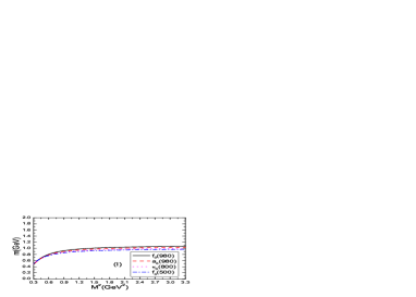
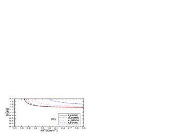
Figure 3: The masses of the scalar mesons as pure tetraquark states with variations of the Borel parameter $M^{2}$, where the (I) and (II) denote the contributions of the condensates $\langle\bar{q}q\rangle\langle\bar{q}^{\prime}g_{s}\sigma Gq^{\prime}\rangle$ of dimension 8 are excluded and included, respectively, $q,q^{\prime}=u,d,s$.

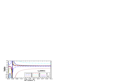
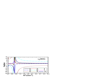
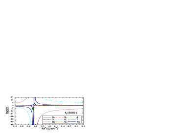
Figure 4: The contributions of different terms in the operator product expansion with variations of the Borel parameter $M^{2}$ for the scalar nonet mesons as pure tetraquark states, where the $0$, $3$, $4$, $5$, $6$, $7$, $8$, $9$ and $10$ denotes the dimensions of the vacuum condensates.

Now we set the mixing angles $\theta_{S}$ to be $90^{\circ}$ in the QCD spectral densities $\rho_{S}(s)$ in Eq.(22), and take the scalar nonet mesons to be pure two-quark states. In Fig.5, we plot the masses of the scalar mesons as pure two-quark states with variations of the Borel parameters $M^{2}$, the same parameters as that in Fig.3 are taken. From the figure, we can see that the predicted masses $m_{S}\approx(0.85-1.14)\,\rm{GeV}$ at the value $M^{2}=(0.5-3.3)\,\rm{GeV}^{2}$, there also exist some difficulty to reproduce the experimental data approximately by fine tuning the continuum threshold parameters. In Fig.6, we plot the contributions of different terms in the operator product expansion with variations of the Borel parameters $M^{2}$ for the scalar nonet mesons as the pure two-quark states. From the figure, we can see that the convergent behavior of the operator product expansion is very good, the main contributions come from the perturbative terms, which are of dimension 6 according to the normalization factors $\langle\bar{q}q\rangle^{2}$ and $\langle\bar{s}s\rangle^{2}$.

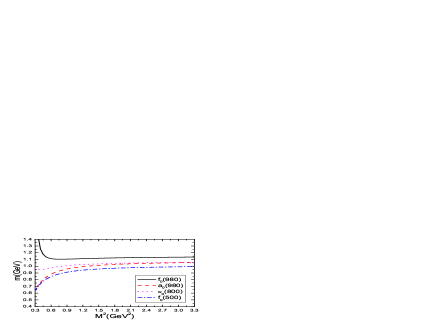
Figure 5: The masses of the scalar mesons as pure two-quark states with variations of the Borel parameter $M^{2}$.

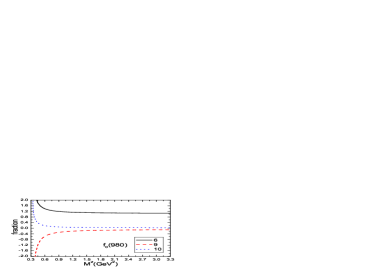
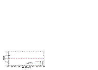
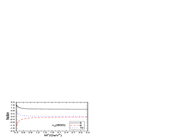
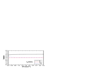
Figure 6: The contributions of different terms in the operator product expansion with variations of the Borel parameter $M^{2}$ for the scalar nonet mesons as pure two-quark states, where the $6$, $9$ and $10$ denotes the dimensions of the vacuum condensates. We have taken into account the normalization factors $\langle\bar{q}q\rangle^{2}$ and $\langle\bar{s}s\rangle^{2}$.

We turn on the mixing angles $\theta_{S}\neq 0^{\circ},\,90^{\circ}$ and take into account all the Feynman diagrams which contribute to the condensate $\langle\bar{q}q\rangle\langle\bar{q}^{\prime}g_{s}\sigma Gq^{\prime}\rangle$ with $q,q^{\prime}=u,d,s$, see the Feynman diagrams in Figs.1-2. The contributions of the vacuum condensates $\langle\bar{q}q\rangle\langle\bar{q}^{\prime}g_{s}\sigma Gq^{\prime}\rangle$ of dimension 8 can be canceled out completely with the ideal mixing angles $\theta^{0}_{S}$,

$$\theta^{0}_{f_{0}(980)} = \tan^{-1}\left(2\frac{\langle\bar{q}q\rangle\langle\bar{s}g_{s}\sigma Gs\rangle+\langle\bar{s}s\rangle\langle\bar{q}g_{s}\sigma Gq\rangle}{\langle\bar{q}q\rangle\langle\bar{q}g_{s}\sigma Gq\rangle}\right)\approx 72.6^{\circ}\,,$$

$$\theta^{0}_{a_{0}(980)} = \tan^{-1}\left(4\frac{\langle\bar{q}q\rangle\langle\bar{s}g_{s}\sigma Gs\rangle+\langle\bar{s}s\rangle\langle\bar{q}g_{s}\sigma Gq\rangle}{\langle\bar{s}s\rangle\langle\bar{s}g_{s}\sigma Gs\rangle}\right)\approx 84.3^{\circ}\,,$$

$$\theta^{0}_{\kappa_{0}(800)} = \tan^{-1}\left(2\frac{2\langle\bar{q}q\rangle\langle\bar{q}g_{s}\sigma Gq\rangle+\langle\bar{q}q\rangle\langle\bar{s}g_{s}\sigma Gs\rangle+\langle\bar{s}s\rangle\langle\bar{q}g_{s}\sigma Gq\rangle}{\langle\bar{q}q\rangle\langle\bar{q}g_{s}\sigma Gq\rangle}\right)\approx 82.1^{\circ}\,,$$

$$\theta^{0}_{f_{0}(500)} = \tan^{-1}\left(4\right)\approx 76.0^{\circ}\,,$$ (37)

which results in much better convergent behavior in the operator product expansion.

In this article, we choose the mixing angles $\theta_{S}=\theta_{S}^{0}$, then impose the two criteria (i.e. pole dominance and convergence of the operator product expansion) of the QCD sum rules on the two-quark-tetraquark mixed states, and search for the optimal values of the Borel parameters $M^{2}$ and continuum threshold parameters $s^{0}_{S}$. The resulting Borel parameters (or Borel windows), continuum threshold parameters and pole contributions of the scalar nonet mesons are shown in Table 2 explicitly.

From Table 2, we can see that the upper bound of the pole contributions can reach $(51-69)\%$, the pole dominance condition is satisfied marginally. If we intend to obtain QCD sum rules for the light tetraquark states with the pole contributions larger than $50\%$, we should resort to multi-pole plus continuum states to approximate the phenomenological spectral densities, include at least the ground state plus the first excited state, and postpone the continuum threshold parameters $s_{S}^{0}$ to much larger values [17]. In this article, we exclude the contaminations of the continuum states by the truncation $s_{S}^{0}$, see Eq.(34), although the truncation $s_{S}^{0}$ cannot lead to the pole contribution larger than (or about) $50\%$ in all the Borel windows. Such a situation is in contrary to the hidden-charm and hidden-bottom tetraquark states and hidden-charm pentaquark states, where the two heavy quarks $Q$ and $\bar{Q}$ stabilize the four-quark systems $q\bar{q}^{\prime}Q\bar{Q}$ and five-quark systems $qq^{\prime}q^{\prime\prime}Q\bar{Q}$, and result in QCD sum rules satisfying the pole dominance condition [25, 26, 27].

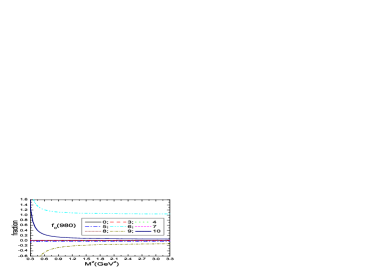
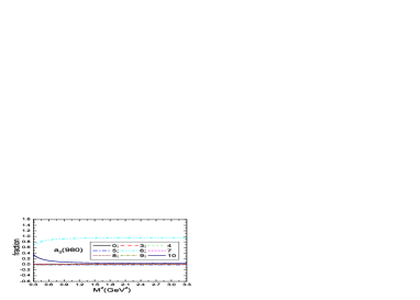
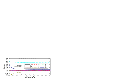
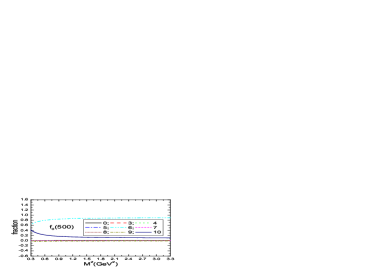
Figure 7: The contributions of different terms in the operator product expansion with variations of the Borel parameter $M^{2}$ for the scalar nonet mesons as two-quark-tetraquark mixed states, where the $0$, $3$, $4$, $5$, $6$, $7$, $8$, $9$ and $10$ denotes the dimensions of the vacuum condensates.

In Fig.7, we plot the contributions of different terms in the operator product expansion with variations of the Borel parameter $M^{2}$ for the scalar nonet mesons as the two-quark-tetraquark mixed states, where the central values of other parameters are taken. From the figure, we can see that the dominant contributions come from the vacuum condensates of dimension 6. The perturbative contributions of the two-quark components $\Pi^{22}_{S}(p)$ of the correlation functions $\Pi_{S}(p)$ are proportional to the vacuum condensate $\langle\bar{q}q\rangle^{2}$ (or $\langle\bar{s}s\rangle^{2}$) of dimension 6 according to the normalization factors $\langle\bar{q}q\rangle$ (or $\langle\bar{s}s\rangle$) in the interpolating currents $J^{2}_{S}(x)$. In the Borel windows, the contributions of the vacuum condensates of dimension 6 are about $(109-114)\%$, $(90-93)\%$, $(107-111)\%$ and $(80-85)\%$ for the $f_{0}(980)$, $a_{0}(980)$, $\kappa_{0}(800)$ and $f_{0}(500)$, respectively; the contributions of the vacuum condensates of dimension 10 are about $(11-16)\%$, $(7-10)\%$, $(19-29)\%$ and $(16-22)\%$ for the $f_{0}(980)$, $a_{0}(980)$, $\kappa_{0}(800)$ and $f_{0}(500)$, respectively, where the total contributions are normalized to be $1$. The operator product expansion is well convergent in the Borel windows shown in Table 2.

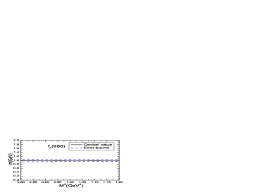
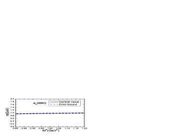
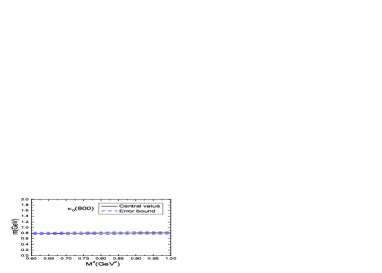
Figure 8: The masses of the scalar nonet mesons as the two-quark-tetraquark mixed states with variations of the Borel parameters.

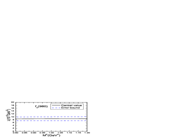
Figure 9: The pole residues of the scalar nonet mesons as the two-quark-tetraquark mixed states with variations of the Borel parameters.

Now we can see that it is reasonable to extract the masses from the QCD sum rules by choosing the Borel parameters and continuum threshold parameters shown in Table 2. In Figs.8-9, we plot the masses and pole residues of the scalar nonet mesons as the two-quark-tetraquark mixed states with variations of the Borel parameters in the Borel windows by taking into account the uncertainties of the input parameters. From the figures, we can see that the platforms are very flat, the predictions are reliable. In Table 3, we present the masses and pole residues of the scalar nonet mesons as the two-quark-tetraquark mixed states, where all uncertainties of the input parameters are taken into account.

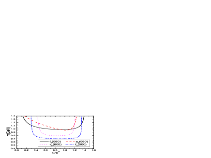
Figure 10: The masses of the scalar mesons as two-quark-tetraquark mixed states with variations of the mixing angle $\theta_{S}$.

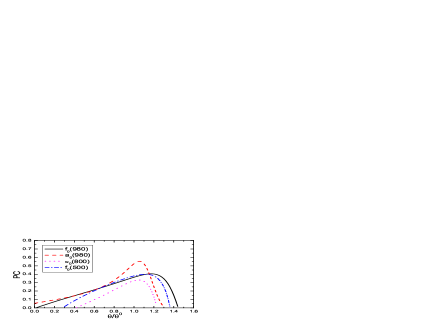
Figure 11: The pole contributions (PC) of the scalar mesons as two-quark-tetraquark mixed states with variations of the mixing angle $\theta_{S}$.

There exists a compromise between the minimal masses and the maximal pole contributions, and in the following two paragraphs we will show that the mixing angles $\theta_{S}^{0}$ are optimal values.

In Fig.10, we plot the masses of the scalar mesons as the two-quark-tetraquark mixed states with variations of the mixing angles $\theta_{S}$, where the input parameters are chosen as $s^{0}_{f_{0}(980)}=1.5\,\rm{GeV}^{2}$, $M^{2}_{f_{0}(980)}=1\,\rm{GeV}^{2}$, $s^{0}_{a_{0}(980)}=1.8\,\rm{GeV}^{2}$, $M^{2}_{a_{0}(980)}=1\,\rm{GeV}^{2}$, $s^{0}_{\kappa_{0}(800)}=1.0\,\rm{GeV}^{2}$, $M^{2}_{\kappa_{0}(800)}=0.8\,\rm{GeV}^{2}$, $s^{0}_{f_{0}(500)}=1.0\,\rm{GeV}^{2}$, $M^{2}_{f_{0}(500)}=0.8\,\rm{GeV}^{2}$, we introduce the subscripts $f_{0}(980)$, $a_{0}(980)$, $\kappa_{0}(800)$ and $f_{0}(500)$ to denote the different Borel parameters. From the figure, we can see that there appear minima in the predicted masses at the values $\theta_{f_{0}(980)}/\theta_{f_{0}(980)}^{0}=0.6-1.2$, $\theta_{a_{0}(980)}/\theta_{a_{0}(980)}^{0}=0.9-1.1$, $\theta_{\kappa_{0}(800)}/\theta_{\kappa_{0}(800)}^{0}=0.6-1.1$, $\theta_{f_{0}(500)}/\theta_{f_{0}(500)}^{0}=0.5-1.2$. The lowest masses of the $f_{0}(980)$ and $a_{0}(980)$ can reproduce the experimental values approximately; while the lowest masses of the $\kappa_{0}(800)$ and $f_{0}(500)$ are larger than the experimental values. In calculations, we observe that the minima of the predicted masses vary with the Borel parameters $M^{2}$ and threshold parameters $s_{S}^{0}$, the mixing angles $\theta_{S}^{0}$ are the best values.

In Fig.11, we plot the pole contributions of the scalar mesons as the two-quark-tetraquark mixed states with variations of the mixing angles $\theta_{S}$, where the same parameters as that in Fig.10 are taken. From the figure, we can see that the pole contributions increase with the $\theta_{S}/\theta_{S}^{0}$ slowly, and reach the maxima at the values $\theta_{S}/\theta_{S}^{0}=1.0-1.3$, then decrease quickly and reach zero approximately. The best values appear at the vicinity of the $\theta_{S}^{0}$, not far way from the $\theta_{S}^{0}$.

We can draw the conclusion tentatively that the QCD sum rules favor the ideal two-quark-tetraquark mixing angles $\theta^{0}_{S}$.

	$M^{2}(\rm{GeV}^{2})$	$s_{0}(\rm{GeV}^{2})$	pole
$f_{0}(980)$	$0.8-1.2$	$1.5\pm 0.1$	$(25-52)\%$
$a_{0}(980)$	$0.8-1.2$	$1.8\pm 0.1$	$(39-69)\%$
$\kappa_{0}(800)$	$0.6-1.0$	$1.0\pm 0.1$	$(20-51)\%$
$f_{0}(500)$	$0.6-1.0$	$1.0\pm 0.1$	$(24-59)\%$

Table 2: The Borel parameters (or Borel windows), continuum threshold parameters and pole contributions of the QCD sum rules for the scalar nonet mesons as the two-quark-tetraquark mixed states.

		$m_{S}(\rm{GeV})$	$\lambda_{S}(10^{-4}\rm{GeV}^{5})$
$f_{0}(980)$		$0.98\pm 0.06$	$8.7\pm 1.3$
$a_{0}(980)$		$0.97\pm 0.05$	$5.0\pm 1.7$
$\kappa_{0}(800)$		$0.80\pm 0.05$	$3.6\pm 0.6$
$f_{0}(500)$		$0.70\pm 0.06$	$5.8\pm 1.0$

Table 3: The masses and pole residues of the scalar nonet mesons as the two-quark-tetraquark mixed states.

Now we study the finite width effects on the predicted masses. For example, the currents $J_{f_{0}/a_{0}(980)}(x)$ couple potentially with the scattering states $K\bar{K}$, we take into account the contributions of the intermediate $K\bar{K}$-loops to the correlation functions $\Pi_{f_{0}/a_{0}(980)}(p^{2})$,

$$\Pi_{f_{0}/a_{0}(980)}(p^{2}) = -\frac{\widehat{\lambda}_{f_{0}/a_{0}(980)}^{2}}{p^{2}-\widehat{m}_{f_{0}/a_{0}(980)}^{2}-\Sigma_{K\bar{K}}(p)}+\cdots\,,$$ (38)

where the $\widehat{\lambda}_{f_{0}/a_{0}(980)}$ and $\widehat{m}_{f_{0}/a_{0}(980)}$ are bare quantities to absorb the divergences in the self-energies $\Sigma_{K\bar{K}}(p)$. All the renormalized self-energies contribute a finite imaginary part to modify the dispersion relation,

$$\Pi_{f_{0}/a_{0}(980)}(p^{2}) = -\frac{\lambda_{f_{0}/a_{0}(980)}^{2}}{p^{2}-m_{f_{0}/a_{0}(980)}^{2}+i\sqrt{p^{2}}\Gamma(p^{2})}+\cdots\,.$$ (39)

The contributions of the other intermediate meson-loops to the correlation functions $\Pi_{S}(p^{2})$ can be studied in the same way.

We can take into account the finite width effects by the following simple replacements of the hadronic spectral densities,

$$\delta\left(s-m^{2}_{S}\right) \to \frac{1}{\pi}\frac{\sqrt{s}\,\Gamma_{S}(s)}{\left(s-m_{S}^{2}\right)^{2}+s\,\Gamma_{S}^{2}(s)}\,.$$ (40)

It is easy to obtain the masses,

$$m_{S}^{2} = \frac{\int_{0}^{s^{0}_{S}}ds\,s\,\frac{1}{\pi}\frac{\sqrt{s}\,\Gamma_{S}(s)}{\left(s-m_{S}^{2}\right)^{2}+s\,\Gamma_{S}^{2}(s)}\,\exp\left(-\frac{s}{M^{2}}\right)}{\int_{0}^{s^{0}_{S}}ds\,\frac{1}{\pi}\frac{\sqrt{s}\,\Gamma_{S}(s)}{\left(s-m_{S}^{2}\right)^{2}+s\,\Gamma_{S}^{2}(s)}\,\exp\left(-\frac{s}{M^{2}}\right)}\,,$$ (41)

where

$$\Gamma_{f_{0}(980)}(s) = \Gamma_{f_{0}(980)}\,,$$

$$\Gamma_{a_{0}(980)}(s) = \Gamma_{a_{0}(980)}\,,$$

$$\Gamma_{\kappa_{0}(800)}(s) = \Gamma_{\kappa_{0}(800)}\frac{m^{2}_{\kappa_{0}(800)}}{s}\,,$$

$$\Gamma_{f_{0}(500)}(s) = \Gamma_{f_{0}(500)}\frac{m^{2}_{f_{0}(500)}}{s}\,,$$ (42)

and the masses $m_{S}$ at the right side of Eq.(41) come from the QCD sum rules in Eq.(34), here we have added the factors $\frac{m^{2}_{\kappa_{0}(800)}}{s}$ and $\frac{m^{2}_{f_{0}(500)}}{s}$ considering the large widths of the $\kappa_{0}(800)$ and $f_{0}(500)$. The numerical results are shown explicitly in Fig.12. From Fig.12, we can see that the predicted masses $m_{f_{0}(980)}$ and $m_{a_{0}(980)}$ are modified slightly after taking into account the small widths $\Gamma_{f_{0}(980)}$ and $\Gamma_{a_{0}(980)}$, the finite widths can be neglected safely; while the predicted masses $m_{\kappa_{0}(800)}$ and $m_{f_{0}(500)}$ are modified considerably with the largest mass-shifts $\delta m_{\kappa_{0}(800)}=-0.09\,\rm{GeV}$ and $\delta m_{f_{0}(500)}=-0.04\,\rm{GeV}$. Now the predicted masses from the QCD sum rules are

$$m_{\kappa_{0}(800)} = (0.71\pm 0.05)\,\rm{GeV}\,,$$

$$m_{f_{0}(500)} = (0.66\pm 0.06)\,\rm{GeV}\,,$$ (43)

which are much better than the values presented in Table 3 compared to the experimental data,

$$m_{\kappa_{0}(800)} = (682\pm 29)\,\rm{MeV}\,,$$

$$m_{f_{0}(500)} = (400-550)\,\rm{MeV}\,,$$ (44)

from the Particle Data Group [1].

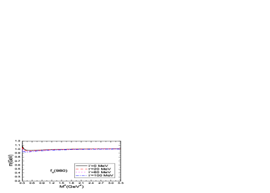
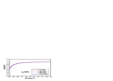
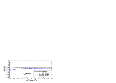
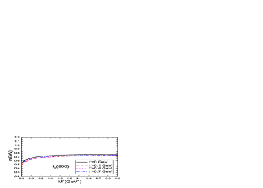
Figure 12: The masses of the scalar nonet mesons with variations of the Borel parameters after taking into account the finite widths.

4 Conclusion

In this article, we assume that the nonet scalar mesons below $1\,\rm{GeV}$ are the two-quark-tetraquark mixed states and study their masses and pole residues using the QCD sum rules. In calculation, we take into account the vacuum condensates up to dimension 10 and the $\mathcal{O}(\alpha_{s})$ corrections to the perturbative terms, and neglect the condensates which are vacuum expectations of the operators of the order $\mathcal{O}(\alpha_{s}^{>1})$, in the operator product expansion. We choose the ideal mixing angles, which can lead to good convergent behavior in the operator product expansion, the resulting two-quark components are much larger than $50\%$. Then we impose the two criteria (i.e. pole dominance and convergence of the operator product expansion) of the QCD sum rules, search for the optimal values of the Borel parameters and continuum threshold parameters, and obtain the masses and pole residues of the nonet scalar mesons. The predicted masses are compatible with the experimental data, while the pole residues can be used to study the hadronic coupling constants and form-factors.

References

[1] K. A. Olive et al, Chin. Phys. C38 (2014) 090001.
[2] F. E. Close and N. A. Tornqvist, J. Phys. G28 (2002) R249.
[3] R. L. Jaffe, Phys. Rept. 409 (2005) 1.
[4] C. Amsler and N. A. Tornqvist, Phys. Rept. 389 (2004) 61.
[5] E. Klempt and A. Zaitsev, Phys. Rept. 454 (2007) 1.
[6] K. Maltman and N. Isgur, Phys. Rev. Lett. 50 (1983) 1827;
K. Maltman and N. Isgur, Phys. Rev. D29 (1984) 952;
N. A. Tornqvist, Phys. Rev. Lett. 67 (1991) 556;
T. E. O. Ericson and G. Karl, Phys. Lett. B309 (1993) 426;
N. A. Tornqvist, Z. Phys. C61 (1994) 525.
[7] J. A. Oller, E. Oset and J. R. Pelaez, Phys. Rev. D59 (1999) 074001.
[8] S. Weinberg, Phys. Rev. Lett. 110 (2013) 261601.
[9] R. L. Jaffe, Phys. Rev. D15 (1977) 267;
R. L. Jaffe, Phys. Rev. D15 (1977) 281;
L. Maiani, F. Piccinini, A. D. Polosa and V. Riquer, Phys. Rev. Lett. 93 (2004) 212002.
[10] F. Giacosa, Phys. Rev. D75 (2007) 054007.
[11] G. ’t Hooft, G. Isidori, L. Maiani, A. D. Polosa and V. Riquer, Phys. Lett. B662 (2008) 424;
A. H. Fariborz, R. Jora and J. Schechter, Phys. Rev. D77 (2008) 094004.
[12] M. A. Shifman, A. I. Vainshtein and V. I. Zakharov, Nucl. Phys. B147 (1979) 385; Nucl. Phys. B147 (1979) 448.
[13] L. J. Reinders, H. Rubinstein and S. Yazaki, Phys. Rept. 127 (1985) 1.
[14] T. V. Brito, F. S. Navarra, M. Nielsen and M. E. Bracco, Phys. Lett. B608 (2005) 69.
[15] Z. G. Wang and W. M. Yang, Eur. Phys. J. C42 (2005) 89;
Z. G. Wang, W. M. Yang and S. L. Wan, J. Phys. G31 (2005) 971.
[16] Z. G. Wang and S. L. Wan, Chin. Phys. Lett. 23 (2006) 3208;
Z. G. Wang, Int. J. Theor. Phys. 51 (2012) 507;
Z. B. Wang and Z. G. Wang, Acta Phys. Polon. B46 (2015) 2467.
[17] Z. G. Wang, Nucl. Phys. A791 (2007) 106.
[18] H. J. Lee, Eur. Phys. J. A30 (2006) 423.
[19] H. X. Chen, A. Hosaka and S. L. Zhu, Phys. Rev. D74 (2006) 054001;
H. X. Chen, A. Hosaka and S. L. Zhu, Phys. Lett. B650 (2007) 369;
H. X. Chen, A. Hosaka and S. L. Zhu, Phys. Rev. D76 (2007) 094025.
[20] J. Sugiyama, T. Nakamura, N. Ishii, T. Nishikawa and M. Oka, Phys. Rev. D76 (2007) 114010.
[21] H. J. Lee and N. I. Kochelev, Phys. Lett. B642 (2006) 358;
H. J. Lee and N. I. Kochelev, Phys. Rev. D78 (2008) 076005;
Y. Pang and M. L. Yan, Eur. Phys. J. A42 (2009) 195;
J. R. Zhang, L. F. Gan and M. Q. Huang, Phys. Rev. D85 (2012) 116007;
J. R. Zhang and G. F. Chen, Phys. Rev. D86 (2012) 116006;
H. J. Lee, N. I. Kochelev and Y. Oh, Phys. Rev. D87 (2013) 117901.
[22] S. Groote, J. G. Körner and D. Niinepuu, Phys. Rev. D90 (2014) 054028.
[23] T. Schafer and E. V. Shuryak, Rev. Mod. Phys. 70 (1998) 323.
[24] P. Colangelo and A. Khodjamirian, hep-ph/0010175.
[25] Z. G. Wang, Int. J. Mod. Phys. A30 (2015) 1550168.
[26] Z. G. Wang and T. Huang, Phys. Rev. D89 (2014) 054019;
Z. G. Wang, Eur. Phys. J. C74 (2014) 2874;
Z. G. Wang and T. Huang, Nucl. Phys. A930 (2014)63.