Exchange splitting of the interaction energy and the multipole expansion of the wave function

Abstract

The exchange splitting $J$ of the interaction energy of the hydrogen atom with a proton is calculated using the conventional surface-integral formula $J_{\textrm{surf}}[\varphi]$, the volume-integral formula of the symmetry-adapted perturbation theory $J_{\textrm{SAPT}}[\varphi]$, and a variational volume-integral formula $J_{\textrm{var}}[\varphi]$. The calculations are based on the multipole expansion of the wave function $\varphi$, which is divergent for any internuclear distance $R$. Nevertheless, the resulting approximations to the leading coefficient $j_{0}$ in the large-$R$ asymptotic series $J(R)=2e^{-R-1}R(j_{0}+j_{1}R^{-1}+j_{2}R^{-2}+\cdots)$ converge, with the rate corresponding to the convergence radii equal to 4, 2, and 1 when the $J_{\textrm{var}}[\varphi]$, $J_{\textrm{surf}}[\varphi]$, and $J_{\textrm{SAPT}}[\varphi]$ formulas are used, respectively. Additionally, we observe that also the higher $j_{k}$ coefficients are predicted correctly when the multipole expansion is used in the $J_{\textrm{var}}[\varphi]$ and $J_{\textrm{surf}}[\varphi]$ formulas. The SAPT formula $J_{\textrm{SAPT}}[\varphi]$ predicts correctly only the first two coefficients, $j_{0}$ and $j_{1}$, gives a wrong value of $j_{2}$, and diverges for higher $j_{n}$. Since the variational volume-integral formula can be easily generalized to many-electron systems and evaluated with standard basis-set techniques of quantum chemistry, it provides an alternative for the determination of the exchange splitting and the exchange contribution of the interaction potential in general.

I Introduction

Multipole expansion of the interaction energy is one of the cornerstones of the theory of atomic interactions Stone:13 ; Jeziorski:94 . It is indispensable for the description of potential energy curves in the domain of large interatomic separations $R$, where it approximates the interaction energy $E_{\textrm{int}}(R)$ asymptotically Ahlrichs:76 ; Morgan:80 as a series in the inverse integer powers of $R$,

$$E_{\textrm{int}}(R)\sim\sum_{n}C_{n}R^{-n},$$ (1)

the coefficients $C_{n}$ being usually referred to as the van der Waals constants. The series on the r.h.s. of Eq. (1) cannot converge to $E_{\textrm{int}}(R)$, since the latter contains also exponentially decaying terms due to charge penetration and resonance tunneling (exchange) of electrons between interacting systems Damburg:84 ; Cizek:86 . Moreover, the multipole expansion (1) is believed to be divergent, although this has been rigorously proved only for H${}_{2}^{+}$ i.e. for the interaction of a hydrogen atom with a proton Damburg:84 ; Graffi:85 ; Cizek:86 and for the second order interaction energy of two hydrogen atoms Young:75 . One may note, however, that the multipole expansion has been proved to converge for interactions of confined atoms Zhang:12 and in calculations with finite basis sets Jansen:00 , although the limits obtained in both these cases differ from the true interaction energy.

The multipole expansion (1) is closely related to and can be obtained from the multipole expansion of the wave function Ahlrichs:76

$$\varphi\sim\varphi_{0}+\sum_{n}R^{-n}\varphi_{n},$$ (2)

where $\varphi_{0}$ is the product of the wave functions of the non-interacting monomers, and $\varphi_{n}$’s are the multipole corrections to the wave function Ahlrichs:76 . The r.h.s. of Eq. (2) does not represent the asymptotic approximation of the exact wave function $\psi$ since it lacks the full permutational and/or spacial symmetry of $\psi$. It has been shown, however, that except for pathological cases Klein:87 , the correct asymptotic expansion of the wave function can be obtained by symmetry projection Ahlrichs:76 , i.e.,

$$\psi={\cal A}\varphi_{0}+\sum_{n=1}^{N}R^{-n}{\cal A}\varphi_{n}+O(R^{-N-1}),$$ (3)

where ${\cal A}$ is the projection operator imposing the appropriate symmetry of the state $\psi$. Equation (3) shows that Eq. (2) provides in fact the asymptotic expansion of a genuine primitive function $\varphi$, as defined, e.g., in Ref. Kutzelnigg:80, . Similarly as the expansion of Eq. (1), the multipole expansions for the wave function, Eq. (3), and for the primitive wave function, Eq. (2), are expected to be divergent in the $L^{2}$ norm (the convergence of the expansion for the wave function would imply the convergence for the interaction energy).

The interaction energies of two or more states have the same asymptotic expansion when they differ only by exponentially small exchange terms. For instance, for the H${}_{2}^{+}$ ion, for the H₂ molecule and alkali dimers, or for homonuclear ions with one electron outside the closed shell, the interaction energies for the lowest gerade and ungerade states can be written as

$${\cal E}_{g,u}(R)=Q(R)\pm J(R),$$ (4)

where $Q(R)$ is the so-called Coulomb energy, assumed to be well represented at large $R$ by the series (1), and $J(R)$ is the so called exchange energy falling off exponentially with $R$ (the + and $-$ signs are used for the $g$ and $u$ states, respectively). The exchange energy $J$ (or the exchange splitting $-2J$) is of paramount importance for the understanding of weak intermolecular interactions Szalewicz:05 , chemical bonds or magnetism Herring:62 , and is relevant experimentally, as it determines the rates of resonant charge exchange processes in slow atomic collisions Galitski:81 ; Smirnov:01 .

The exchange energy $J(R)$ and its large $R$ asymptotic expansion are much more difficult to calculate than the long-range part of the interaction energy, given by Eq. (1). This is due to the fact that $J(R)$, as a tunneling effect, is sensitive to the values of wave functions in the classically forbidden region of the configuration space, where the wave function amplitudes are very small and are hard to determine accurately using the conventional techniques of electronic structure theory. Instead of the wave functions $\psi_{g}$ and $\psi_{u}$, it is more convenient to work with a primitive function Kutzelnigg:80 $\varphi$, such that $\psi_{g}={\cal A}_{g}\varphi$, and $\psi_{u}={\cal A}_{u}\varphi$, where ${\cal A}_{g}$, and ${\cal A}_{u}$ are appropriate symmetry projectors. When $\varphi$ is known, $J(R)$ can be obtained from the surface integral formula Firsov:51 ; Holstein:52 ; Herring:62 ,

$$J_{\textrm{surf}}[\varphi]=\frac{-\int_{M}\varphi\mathbf{\nabla}\varphi\textrm{d}\mathbf{S}}{\langle\varphi|\varphi\rangle-2\int_{\textrm{right}}\varphi^{2}\textrm{d}V},$$ (5)

where $M$ indicates the median plane of the molecule, and the volume integral in the denominator is taken over the half of the space right to $M$ ($\varphi$ is understood to be localized on the left of $M$). Atomic units are used in Eq. (5) and throughout the paper. The surface-integral method has been extended to hydrogen molecule Gorkov:64 ; Herring:64 ; Burrows:12 alkali-metal dimer cations Smirnov:65 ; Bardsley:75 ; Tang:92 ; Scott:02 ; Scott:04 ; Jamieson:09 ; Burrows:10 , neutral homo- and heterodimers Kleinekathoefer:96 ; Kleinekathoefer:00 ; Scott:04b ; Yiu:11 ; Chen:14 , excited states of H${}_{2}^{+}$ ion Scott:91 , and interactions of diatomic molecules with atomic ions Khoma:08 . For the discussion of other extensions of this theory see Ref. Chibisov:88, .

In our previous work Gniewek:14 we presented a volume integral formula for $J(R)$ rooted in the Symmetry Adapted Perturbation Theory (SAPT),

$$J_{\textrm{SAPT}}[\varphi]=\frac{\langle\varphi_{0}|VP\varphi\rangle\langle\varphi_{0}|\varphi\rangle-\langle\varphi_{0}|V\varphi\rangle\langle\varphi_{0}|P\varphi\rangle}{\langle\varphi_{0}|\varphi\rangle^{2}-\langle\varphi_{0}|P\varphi\rangle^{2}},$$ (6)

where $V$ is the operator collecting Coulombic interactions of particles of one monomer with those of the other, and $P$ is the operator inverting the electronic coordinates with respect to the midpoint of the internuclear axis (for H${}_{2}^{+}$ and H₂) or permuting electrons between monomers (for larger systems). When $\varphi$ is approximated via basis set expansions or via the expansion in powers of the interaction operator $V$, the formula of Eq. (6) was shown to give much better results Gniewek:14 than the surface-integral formula (5). In fact, with $\varphi$ expanded in powers of $V$, the formula (6) gives the expansion of the exchange energy in the symmetrized Rayleigh-Schrödinger (SRS) perturbation theory Jeziorski:78 , which forms the basis for the calculation of exchange effects in most of the practical implementations of SAPT Szalewicz:12 ; Sherrill:12 ; Jansen:14 ; Hesselmann:14 .

In this communication we consider another volume-integral formula, which is variational in its origin, and, as we shall show, surpasses $J_{\textrm{surf}}[\varphi]$ and $J_{\textrm{SAPT}}[\varphi]$ in accuracy,

$$J_{\textrm{var}}[\varphi]=\frac{\langle\varphi|HP\varphi\rangle\langle\varphi|\varphi\rangle-\langle\varphi|H\varphi\rangle\langle\varphi|P\varphi\rangle}{\langle\varphi|\varphi\rangle^{2}-\langle\varphi|P\varphi\rangle^{2}}.$$ (7)

A similar expression and its simplified forms have been considered in the literature Galitski:81 ; Janev:81 ; Chibisov:88 ; Khoma:08 in the theory of resonant and non-resonant atom-ion charge exchange processes (Landau-Zener theory) but not in the present context of accurate ab initio calculations of the exchange energy.

The purpose of the present work is to investigate the performance of the surface-integral formula, Eq. (5), and the two volume-integral formulas, Eqs. (6), and (7), in the prediction of the exchange splitting energy $J(R)$ when the primitive function $\varphi$ is represented by the multipole expansion, of Eq. (2). Since the error of the asymptotic series (3) truncated after the $N$th term is the order of $R^{-N-1}$, it is not obvious that this series can be useful to correctly generate the exponentially small exchange terms in the energy. In fact is has been argued Harrell:80 that “it is hopeless to try to compute the splitting by any perturbative series expansion in $1/R$”. On the other hand, such a procedure, if successful, would be attractive computationally since the expansion (2) is relatively easy to generate and Eq. (3) provides the simplest approximation to the wave function that is asymptotically correct in the whole configuration space.

The performance of different approximations of $J(R)$ can be best investigated for the H${}_{2}^{+}$ molecular ion. For this simplest, archetypal system the exchange energy can be computed from the exactly known asymptotic expansion Ovchinnikov:65 ; Komarov:67 ; Damburg:68 ; Cizek:86 :

$$J(R)=2e^{-R-1}R(j_{0}+j_{1}/R+j_{2}/R^{2}+j_{3}/R^{3}+\cdots).$$ (8)

Čížek et al. gave accurate values of the first 52 $j_{k}$’s in Ref. Cizek:86, . For the interaction of two hydrogen atoms only the first term in the analogous expansion is known Gorkov:64 ; Herring:64 , although even the functional form of this leading term has been debated recently Burrows:12 . For larger systems only approximate form of the leading term is known Smirnov:65 ; Bardsley:75 ; Tang:92 ; Scott:02 ; Scott:04 ; Jamieson:09 ; Burrows:10 ; Kleinekathoefer:96 ; Kleinekathoefer:00 ; Scott:04b ; Yiu:11 ; Chen:14 . Its accuracy is hard to ascertain since no reference data sufficiently accurate at large $R$ are available. Therefore, we performed our investigation for the H${}_{2}^{+}$ molecular ion and compared our results with the exact formula of Eq. (8).

The problem considered by us was first studied by Tang, Toennies, and Yiu Tang:91 who evaluated the surface integral (5) with $\varphi$ represented by the multipole expansion of the Rayleigh-Schrödinger (RS) perturbation series in $V$ (the polarization expansion Jeziorski:94 ; Hirschfelder:67 ). They were able to sum this series to infinite order and have shown that the first, $j_{0}$ term in Eq. (8) is obtained correctly in this way. They also obtained reasonably good approximate values of $j_{1}$ and $j_{2}$ by representing $\varphi$ through the second order in $V$. These authors did not consider the alternative, volume-integral formulas.

It may be noted that for H${}_{2}^{+}$ the exchange energy $J(R)$ can be approximately obtained directly from the series (1) without using the wave function expansion of Eq. (2). Brezin and Zinn-Justin Brezin:79 have shown that the large $n$ behavior of the van der Waals constants $C_{n}$ in of Eq. (1) is related to the exchange energy via the relation

$$C_{n}\approx-\int_{0}^{\infty}\!\!\!R^{n-1}[J(R)]^{2}\,\textrm{d}R.$$ (9)

Inserting the expansion (8) into Eq. (9), performing integration over $R$, and comparing with the known $1/n$ expansion of $C_{n}$ Morgan:80 ; Cizek:80 ,

$$C_{n}=-\frac{1}{e^{2}}\frac{(n+1)!}{2^{n}}\bigg{(}1+\frac{2}{n}-\frac{20}{n^{2}}+O\big{(}n^{-3}\big{)}\bigg{)}.$$ (10)

one finds the correct values of $j_{0}=-1$ and $j_{1}=-1/2$, while for $j_{2}$ an incorrect value of 19/8 is obtained, 24%  smaller than the accurate value of $j_{2}$ equal to 25/8. Thus only the first two terms in the expansion (8) can be obtained exactly in this way. This method requires the knowledge of an analytic form of the $n$ dependence of $C_{n}$, which can hardly be expected to be available for larger systems.

The organization of the paper is as follows. In Sec. II we define the multipole and polarization expansions of the primitive function, discuss their applications to the evaluation of the asymptotics of the exchange energy and derive analytically the series representation for $j_{0}$ predicted by the SAPT’s volume-integral formula. In Sec. III we present numerical results obtained with the large-order multipole expansion of the primitive function and with the first-order polarization wave function. A successful application of a simple variational approximation to the primitive function is also presented. Finally, in Sec. IV we present conclusions of our investigation.

II Theory

II.1 Primitive function and the variational volume-integral formula

A primitive function $\varphi$ Kutzelnigg:80 ; Hirschfelder:67 is a nontrivial linear combination of the asymptotically degenerate wave functions $\psi_{g}$ and $\psi_{u}$ of the gerade and ungerade states,

$$\varphi=c_{1}\psi_{g}+c_{2}\psi_{u},$$ (11)

from which these exact states can be recovered by projection

$$\psi_{g}=\tfrac{1}{2}(1+P)\varphi,\quad\ \ \psi_{u}=\tfrac{1}{2}(1-P)\varphi.$$ (12)

We shall also require that $\varphi$ is a “genuine primitive function” Kutzelnigg:80 , i.e., that it is localized in the same way as $\varphi_{0}$. This means that $\langle\varphi|P\varphi\rangle$ vanishes exponentially or, more rigorously, that

$$\langle\varphi|P\varphi\rangle=o(R^{-n})$$ (13)

for all integers $n>0$.

Substituting the wave functions of the form given by Eq. (12) in the Rayleigh-Ritz functional and taking into account that $[H,P]\!=\!0$ and $(1\pm P)^{2}\sim 1\pm P$ one finds

$$E_{g}\!-\!E_{u}\!=\!\frac{\langle\varphi|H\varphi\rangle\!+\!\langle\varphi|H\!P\varphi\rangle}{\langle\varphi|\varphi\rangle\!+\!\langle\varphi|P\varphi\rangle}\!-\!\frac{\langle\varphi|H\varphi\rangle\!-\!\langle\varphi|H\!P\varphi\rangle}{\langle\varphi|\!\varphi\rangle\!-\langle\varphi|P\varphi\rangle}.$$ (14)

When the subtraction in Eq. (14) is carried out analytically, the $R$ independent and the long-range $R^{-n}$ terms in the numerator cancel out in view of Eq. (13) and one obtains Eq. (7) for the exponentially vanishing energy splitting $J(R)$. The explicit form of the non-relativistic Hamiltonian $H$ of the hydrogen atom at point $a$ interacting with a proton at point $b$ is $H=H_{0}+V$, where

$$H_{0}=-\frac{1}{2}\nabla^{2}-\frac{1}{r_{a}},\quad\quad V=-\frac{1}{r_{b}}+\frac{1}{R},$$ (15)

$r_{a}$ and $r_{b}$ denoting the electron-nucleus distances. The operator $V$ of Eq. (15) appears in the SAPT formula of Eq. (6).

II.2 Multipole expansion of the primitive function

The multipole expansion of the primitive function $\varphi$, Eq. (2), is obtained if the operator $V$ is represented as the sum of charge-multipole interactions

$$V\sim \ R^{-2}\,V_{2}+R^{-3}\,V_{3}+R^{-4}\,V_{4}+\ldots,$$ (16)

$$V_{n}=-r_{a}^{n-1}P_{n-1}(\cos\theta_{a}),$$ (17)

where $P_{n}(x)$ is the Legendre polynomial and $\theta_{a}$ is the polar angle at nucleus $a$. The expansion of the eigenfunctions of $H_{0}+V$ in powers of $R^{-1}$ leads then to the following recurrence equations for the van der Waals constants $C_{n}$ and multipole corrections to the wave function $\varphi_{n}$:

$$C_{n}=\sum_{m=2}^{n}\langle\varphi_{0}|V_{m}\varphi_{n-m}\rangle,$$ (18)

$$(H_{0}-E_{0})\varphi_{n}=\sum_{m=2}^{n}(C_{m}-V_{m})\varphi_{n-m},$$ (19)

where $E_{0}=-\frac{1}{2}$ and $\varphi_{0}=\pi^{-1/2}e^{-r_{a}}$ are the ground-state energy and the wave function of the unperturbed hydrogen atom. To specify $\varphi_{n}$ uniquely we assumed here the intermediate normalization condition of $\varphi$, i.e., $\langle\varphi_{0}|\varphi\rangle=1$ or, equivalently, $\langle\varphi_{0}|\varphi_{n}\rangle=0$ for $n>0$.

One can show by induction that $\varphi_{n}$ is a product of $\varphi_{0}$ and a polynomial in $r_{a}$ and $\cos\theta_{a}$. The functions $\varphi_{2}$ and $\varphi_{3}$ consist of only one partial wave each, $p$ and $d$, respectively, while the higher ones contain more than one partial-wave component. We calculated the van der Waals constants $C_{n}$ and wave function corrections $\varphi_{n}$ up to $n$=150 using a computer algebra program. We employed the exact representations of rational numbers, so the calculated $C_{n}$ and $\varphi_{n}$ are exact.

II.3 Polarization expansion of the primitive function

Another useful approximation to the primitive function is obtained by a finite order polarization expansionHirschfelder:67 (or polarization approximation). This is an application of the standard Rayleigh-Schrödinger perturbation theory to the Hamiltonian partitioning $H=H_{0}+V$, resulting in the expansion of $\varphi$ in powers of $V$,

$$\varphi=\sum_{k=0}^{\infty}\varphi^{(k)}.$$ (20)

The individual terms in this expansion can be obtained from the equation

$$(H_{0}-E_{0})\varphi^{(k)}=-V\varphi^{(k-1)}+\sum_{j=1}^{k}E^{(j)}\varphi^{(k-j)},$$ (21)

where $E^{(k)}=\langle\varphi_{0}|V\varphi^{(k-1)}\rangle$, and the recursive process is initiated assuming $\varphi^{(0)}=\varphi_{0}$ and $E^{(0)}=E_{0}$. To fully specify $\varphi^{(k)}$ we also assume the intermediate normalization of $\varphi$, i.e., $\langle\varphi_{0}|\varphi^{(k)}\rangle=0$ for $k>0$. For H${}_{2}^{+}$ only the first-order term, $\varphi^{(1)}$, in the series (20) is known in the closed form Dalgarno:57 .

For systems like H${}_{2}^{+}$ or H₂ the polarization expansion has been demonstrated numerically to converge to the wave function of the ground, gerade state Chalasinski:77 ; Tang:94 , although for large $R$ the convergence radius is only marginally greater than unity Gniewek:14 ; Cwiok:92:pol ; Kutzelnigg:92 and the convergence rate becomes prohibitively poor. Thus, at infinite order the sum of the series (20) does not represent a genuine primitive function since it does not satisfy neither the second Eq. (12) nor the locality condition of Eq. (13). Nevertheless the polarization expansion (20) provides an asymptotic approximation of the primitive function in the sense that Ahlrichs:76 ; Jeziorski:82

$$\psi_{\nu}={\cal A}\Phi^{(K)}+O(R^{-\kappa(K+1)}),$$ (22)

where $\Phi^{(K)}$ is the sum of the first $K+1$ terms in Eq. (20), ${\cal A}$ is a suitable symmetry projector, $(1\pm P)/2$ in the case of H${}_{2}^{+}$, and $\kappa=2$, when at least one of interacting subsystems is charged and $\kappa=3$ otherwise.

Each term in Eq. (20) can be represented by the multipole expansion in powers of $R^{-1}$,

$$\varphi^{(k)}\sim\sum_{n}R^{-n}\,\varphi^{(k)}_{n}.$$ (23)

The series on the r.h.s. of (23) cannot converge in the whole configuration space but is expected to provide the large-$R$ asymptotic expansion of $\varphi^{(k)}$ in the $L^{2}$ norm. Dalgarno and Lewis Dalgarno:55 have shown that

$$\varphi^{(1)}\sim\sum_{n=2}^{\infty}R^{-n}\left(\frac{r_{a}^{n-1}}{n-1}+\frac{r_{a}^{n}}{n}\right)\,\varphi_{0}\,P_{n-1}(\cos\theta_{a}).$$ (24)

For $k>1$ the coefficients $\varphi^{(k)}_{n}$, similarly as $\varphi_{n}$, are products of polynomials in $r_{a}$ and $\cos\theta_{a}$ and the function $\varphi_{0}$. One can easily show that

$$\varphi_{n}=\sum_{k=1}^{[n/2]}\varphi^{(k)}_{n},$$ (25)

where $[r]$ denotes the entire value of $r$. Eq. (25) may be viewed as the expansion of $\varphi_{n}$ in powers of $V$, i.e., the polarization expansion of $\varphi_{n}$. We shall also need the multipole expansion of $\Phi^{(K)}$ truncated after the $R^{-N}$ term

$$\Phi^{(K)}_{N}=\sum_{k=0}^{K}\sum_{n=0}^{N}\,R^{-n}\,\varphi^{(k)}_{n}.$$ (26)

Note that for $K\geq N/2$ we have $\Phi_{N}^{(K)}=\Phi_{N}$, where

$$\Phi_{N}=\sum_{n=0}^{N}R^{-n}\varphi_{n}.$$ (27)

is the the multipole expansion of Eq. (2) truncated after the $R^{-N}$ term.

II.4 SAPT expansion of $j_{0}$

In this subsection we shall use the SAPT formula $J_{\textrm{SAPT}}[$$\varphi$] and the multipole expansion for $\varphi$, Eq. (2), to analytically evaluate the leading $j_{0}$ term in Eq. (8). It is easy to see that in evaluating $j_{0}$, the second term in the numerator of Eq. (6) can be neglected and the denominator can be replaced by 1. Thus, in view of Eq. (2), $j_{0}$ can be obtained by analyzing the large $R$ asymptotics of the expression $\langle\,\varphi_{0}|VP\Phi_{N}\,\rangle$ or its individual terms $R^{-n}\langle\,\varphi_{0}|VP\varphi_{n}\,\rangle$. The function $\varphi_{n}$ can be written as a product of $\varphi_{0}$ and a polynomial $f_{n}$ in $r_{a}$ and $\cos\theta_{a}$, i.e., $\varphi_{n}=f_{n}\varphi_{0}$, where $f_{0}=1$, $f_{1}=0$ and

$$f_{n}(r_{a},\cos\theta)=\sum_{l=0}^{n-1}\sum_{m=0}^{n}d_{nml}\,r_{a}^{m}P_{l}(\cos\theta_{a})$$ (28)

for $n\geq 2$. Employing the prolate spheroidal coordinates coordinates $\xi=(r_{a}+r_{b})/R$ , $\eta=(r_{a}-r_{b})/R$ and integrating by parts one finds that

$$\langle\varphi_{0}|V P\varphi_{0}f_{n}\rangle=\frac{1}{4}Re^{-R}\bigg{[}\int_{-1}^{1}v(1,\eta)d\eta$$ (29)

$$+R^{-1}\int_{-1}^{1}\frac{dv(\xi,\eta)}{d\xi}\bigg{|}_{\xi=1}d\eta+O(R^{-2})\bigg{]},$$

where

$$v(\xi,\eta)=\big{(}\xi+\eta\big{)}(\xi-\eta-2)\,f_{n}\big{(}\tfrac{R(\xi-\eta)}{2},\tfrac{1-\xi\eta}{\xi-\eta}\big{)}.$$ (30)

Eqs. (29) and (30) show that the leading asymptotic term of $J_{\textrm{SAPT}}[$$f_{n}\varphi_{0}$] depends only on the values of $f_{n}$ for $\xi=1$, i.e. on the values of $f_{n}$ on the line joining the nuclei $a$ and $b$. On this line $\theta_{b}=0$ and $P_{l}(\cos\theta_{b})=1$. Thus, the sought-after asymptotics in unchanged if the function $f_{n}(r_{a},\cos\theta)$ is replaced by

$$f_{n}(r_{a},1)=\sum_{m=0}^{n}d_{nm}\,r_{a}^{m},$$ (31)

where

$$d_{nm}=\sum_{l=0}^{n-1}d_{nml}.$$ (32)

By inspecting Eqs. (29) and (30) one can also see that the leading contribution to $\langle\varphi_{0}|VP\varphi_{0}f_{n}\rangle$ comes from the highest, $m=n$, power in Eq. (31). Thus, to evaluate the leading asymptotics of $J_{\textrm{SAPT}}[$$f_{n}\varphi_{0}$] one can replace the complete expression for $f_{n}$ by $d_{n}r_{a}^{n}$, where $d_{nn}$ is denoted by $d_{n}$ for brevity.

Inserting Eq. (28) into Eq. (19), setting $\theta=0$ and comparing coefficients at the highest power of $r_{a}$ one obtains the following recurrence relation

$$nd_{n}=d_{0}+d_{1}+d_{2}+\cdots+d_{n-2}.$$ (33)

Using Eq. (33) one can easily prove that

$$d_{n}-d_{n-1}=-\frac{1}{n}\big{(}d_{n-1}-d_{n-2}\big{)}.$$ (34)

Taking also into that $d_{0}=1$ and $d_{1}=0$ one obtains

$$d_{n}-d_{n-1}=\frac{(-1)^{n}}{n!},$$ (35)

and, consequently,

$$d_{n}=\sum_{m=0}^{n}\frac{(-1)^{m}}{m!}.$$ (36)

In view of Eqs. (29) and (30) the leading asymptotics of $\langle\varphi_{0}|VPr_{a}^{n}\varphi_{0}\rangle$ is given by

$$\frac{-R^{n+1}e^{-R}}{2^{n+2}}\!\!\int_{-1}^{1}(1+\eta)^{2}(1-\eta)^{n}d\eta=\frac{-4R^{n+1}e^{-R}}{(n+1)(n+2)(n+3)}.$$ (37)

Summing up contributions from $\varphi_{0}$ up to $\varphi_{N}$ we find that the large $R$ asymptotics of $J_{\textrm{SAPT}}[$$\Phi_{N}$] is given by

$$\sum_{n=0}^{N}\,\frac{-4d_{n}}{(n+1)(n+2)(n+3)}\,Re^{-R}.$$ (38)

Since the $d_{n}$ coefficients converge quickly to $1/e$ it is clear that the series (38) converges, although slowly, with the d’Alembert ratio $|a_{n+1}/a_{n}|$ equal $1-3n^{-1}+O(n^{-2})$, i.e., with the corresponding convergence radius equal to unity. To evaluate its limit one can use the obvious identity

$$p_{n}(q_{n+1}-q_{n})=p_{n+1}q_{n+1}-p_{n}q_{n}-(p_{n+1}-p_{n})q_{n+1},$$ (39)

valid for arbitrary sequences $p_{n}$ and $q_{n}$. Setting

$$p_{n}=d_{n},\quad\quad q_{n}=\frac{2}{(n+1)(n+2)},$$ (40)

and summing both sides of Eq. (39) over $n$ from $n=0$ up to $n=N$ we find

$$\sum_{n=0}^{N} \frac{-4d_{n}}{(n+1)(n+2)(n+3)}=$$ (41)

$$=\frac{2d_{N+1}}{(N+2)(N+3)}-1-2\sum_{n=0}^{N}\frac{(-1)^{n-1}}{(n+3)!},$$

where we took into account that $d_{0}=1$, $q_{0}=1$ and $d_{n+1}-d_{n}=(-1)^{n+1}/(n+1)!$. When $N\rightarrow\infty$ the first term on the r.h.s. vanishes and the last one has the limit equal to $-2/e+1$. Thus, the series on the l.h.s. converges to $2/e$ and one finds that $J_{\textrm{SAPT}}[$$\Phi_{N}$] gives the correct asymptotics of $J(R)$ corresponding to $j_{0}=-1$. Having in mind that the multipole expansion of the wave function, Eq. (2), leads to the divergent expansion for the total interaction energy we find it quite remarkable that, when inserted into the SAPT formula $J_{\textrm{SAPT}}[$$\phi$], this expansion gives the convergent series for such a subtle effect as the asymptotic exchange splitting $(-2/e)Re^{-R}$.

III Numerical Results

III.1 Exchange splitting from the multipole expansion of the primitive function

Since the functions $f_{n}$ are polynomials in $r_{a}$ and $\cos\theta_{a}$, the exchange splittings $J_{\textrm{SAPT}}[\Phi_{N}]$, $J_{\textrm{surf}}[\Phi_{N}]$ and $J_{\textrm{var}}[\Phi_{N}]$ can be obtained in a closed form for a wide range of $N$ employing computer algebra software. For instance, for $N=3$ we obtained

$$J_{\textrm{surf}}[\Phi_{3}]=Re^{-R}(-\tfrac{49}{72}-\tfrac{7}{16}\tfrac{1}{R}+\tfrac{613}{384}\tfrac{1}{R^{2}}+\cdots),$$ (42)

$$J_{\textrm{SAPT}}[\Phi_{3}]=Re^{-R}\big{(}-\tfrac{32}{45}-\tfrac{7}{30}\tfrac{1}{R}+\tfrac{97}{60}\tfrac{1}{R^{2}}+\cdots),$$ (43)

$$J_{\textrm{var}}[\Phi_{3}]=Re^{-R}\big{(}-\tfrac{4147}{5670}-\tfrac{1369}{3780}\tfrac{1}{R}+\tfrac{17239}{7560}\tfrac{1}{R^{2}}+\cdots).$$ (44)

Comparing with Eq. (8) we see that after multiplication by $e/2$ the successive coefficients at $1/R^{k}$ on the r.h.s. of Eqs. (42)-(44) represent approximations to the $j_{k}$ coefficients in the expansion (8). These coefficients computed using the function $\Phi_{N}$ and the appropriate energy expressions will be denoted by $j_{k}^{\textrm{surf}}[\Phi_{N}]$, $j_{k}^{\textrm{SAPT}}[\Phi_{N}]$, and $j_{k}^{\textrm{var}}[\Phi_{N}]$. In view of Eqs. (42)-(44), for $N=3$ the corresponding approximations to the $j_{0}$ coefficient are $-49e/144$, $-16e/45$, and $-4147e/11340$, and differ from the exact value $j_{0}=-1$ by 7.5%, 3.3%, and 0.6%, respectively.

In Tables 1, 2, and 3 we show how the values of $j_{0}$, $j_{1}$, and $j_{2}$ computed from $\Phi_{N}$ converge when $N$ increases (the rows for $N=1$ are absent since $\varphi_{1}=0$ so that $\Phi_{1}=\Phi_{0}$). For the constants $j_{0}$, $j_{1}$, and $j_{2}$ the fastest convergence by far is observed in the case of the variational formula, whereas the SAPT formula gives the slowest convergence. Moreover, the sequence $j_{2}^{\textrm{SAPT}}[\Phi_{N}]$ converges to a spurious value of $55/24\approx 2.292$, instead of the correct one, equal to 25/8 = 3.125. We also observed that for $k\geq 3$ the sequences $j_{k}^{\textrm{SAPT}}[\Phi_{N}]$ diverge while the sequences generated by the surface-integral and variational formulas appear to be convergent for all constants $j_{k}$ that we computed. In the case of the variational formula this convergence is demonstrated numerically for $k\leq 6$ in Table 4. It can be seen that the variational volume formula provides excellent accuracy also for further terms in the expansion of Eq. (8).

Table 1: Values of $j_{0}$ calculated from the surface- and volume-integral formulas with the multipole expansion of Eq. (2) truncated after the $R^{-N}\varphi_{N}$ term.

$N$	$-j_{0}^{\textrm{SAPT}}$	$-j_{0}^{\textrm{surf}}$	$-j_{0}^{\textrm{var}}$
0	$0.9061$	$0.6796$	$0.9060\ 9394$
2	$0.9514$	$0.8601$	$0.9805\ 2309$
3	$0.9665$	$0.9250$	$0.9940\ 6656$
4	$0.9762$	$0.9625$	$0.9984\ 1193$
5	$0.9821$	$0.9811$	$0.9995\ 7106$
6	$0.9861$	$0.9905$	$0.9998\ 8567$
7	$0.9889$	$0.9953$	$0.9999\ 6973$
8	$0.9909$	$0.9976$	$0.9999\ 9204$
9	$0.9924$	$0.9988$	$0.9999\ 9791$
10	$0.9936$	$0.9994$	$0.9999\ 9946$
$\infty$	$1.0$	$1.0$	$1.0$

Table 2: Values of $j_{1}$ calculated from the surface- and volume-integral formulas with the multipole expansion of Eq. (2) truncated after the $R^{-N}\varphi_{N}$ term.

$N$	$-j_{1}^{\textrm{SAPT}}$	$-j_{1}^{\textrm{surf}}$	$-j_{1}^{\textrm{var}}$
0	$0.0$	$0.0$	$0.0$
2	$0.272$	$0.573$	$0.465\ 99$
3	$0.317$	$0.595$	$0.492\ 24$
4	$0.362$	$0.632$	$0.503\ 58$
5	$0.388$	$0.612$	$0.502\ 63$
6	$0.407$	$0.585$	$0.501\ 28$
7	$0.420$	$0.559$	$0.500\ 52$
8	$0.430$	$0.539$	$0.500\ 19$
9	$0.438$	$0.525$	$0.500\ 07$
10	$0.445$	$0.515$	$0.500\ 02$
$\infty$	$0.5$	$0.5$	$0.5$

Table 3: Values of $j_{2}$ calculated from the surface- and volume-integral formulas with the multipole expansion of Eq. (2) truncated after the $R^{-N}\varphi_{N}$ term. The exact value of $j_{2}$ is 25/8. The sequence $j_{2}^{\textrm{SAPT}}[\Phi_{N}]$ converges to the incorrect value equal to $55/24\approx 2.292$.

$N$	$j_{2}^{\textrm{SAPT}}$	$j_{2}^{\textrm{surf}}$	$j_{2}^{\textrm{var}}$
0	$1.359$	$0.0$	$1.359\ 14$
2	$1.925$	$1.083$	$2.626\ 05$
3	$2.197$	$2.170$	$3.099\ 24$
4	$2.218$	$2.666$	$3.147\ 05$
5	$2.254$	$3.099$	$3.156\ 90$
6	$2.269$	$3.318$	$3.146\ 38$
7	$2.278$	$3.409$	$3.136\ 55$
8	$2.284$	$3.417$	$3.130\ 49$
9	$2.288$	$3.384$	$3.127\ 39$
10	$2.291$	$3.334$	$3.125\ 97$
$\infty$	$2.292$	$3.125$	$3.125$

The convergence of the sequence $j_{0}^{\textrm{SAPT}}[\Phi_{N}]$, shown in Table 1, to the correct limit is proved in Sec. II.4, while for the sequence $j_{0}^{\textrm{surf}}[\Phi_{N}]$ the proof of convergence can be found in Ref. Tang:91, . A rigorous mathematical proof that the sequence $j_{0}^{\textrm{var}}[\Phi_{N}]$, shown in the last column of Table 1, converges to the correct limit is more complicated Gniewek:15 and is beyond the scope of the present communication. The convergence of the sequences presented in Tables 2 and 3, as well as their limits have been established numerically based on the calculations for very high values of $N$.

Table 4: Values of the coefficients $j_{k}$, $k\leq 6$, calculated from the variational formula and the multiple expansion of the primitive wave function, Eq. (2), truncated after $n=10$, 20, and 30. Data are rounded to show two digits differing from the exact value. The exact values are taken from Ref. Cizek:86, .

$k$	$j_{k}^{\textrm{var}}[\Phi_{10}]$	$j_{k}^{\textrm{var}}[\Phi_{20}]$	$j_{k}^{\textrm{var}}[\Phi_{30}]$	$j_{k}$
0	$-0.999\ 999\ 46$	$-0.999\ 999\ 999\ 999\ 30$	$-0.999\ 999\ 999\ 999\ 999\ 999\ 20$	$-1.$
1	$-0.500\ 022$	$-0.500\ 000\ 000\ 13$	$-0.500\ 000\ 000\ 000\ 000\ 35$	$-0.5$
2	$3.125\ 97$	$3.125\ 000\ 022$	$3.125\ 000\ 000\ 000\ 13$	$3.125$
3	$2.708$	$2.729\ 164\ 0$	$2.729\ 166\ 666\ 628$	$2.729\ 166\ 666\ 667$
4	$10.46$	$10.216\ 39$	$10.216\ 145\ 842$	$10.216\ 145\ 833$
5	$38.9$	$37.847$	$37.864\ 321\ 3$	$37.864\ 322\ 9$
6	$65.$	$114.1$	$113.263\ 89$	$113.263\ 65$

To characterize the convergence rates of the sequences shown in Tables 1-3, we computed the increment ratios $\rho_{N}(j^{\textrm{SAPT}}_{k})$, $\rho_{N}(j^{\textrm{surf}}_{k})$, and $\rho_{N}(j^{\textrm{var}}_{k})$ defined as

$$\rho_{N}(j^{\textrm{SAPT}}_{k})=-\frac{j_{k}^{\textrm{SAPT}}[\Phi_{N-1}]-j_{k}^{\textrm{SAPT}}[\Phi_{N}]}{j_{k}^{\textrm{SAPT}}[\Phi_{N+1}]-j_{k}^{\textrm{SAPT}}[\Phi_{N}]}$$ (45)

and similarly for $\rho_{N}(j^{\textrm{surf}}_{k})$, and $\rho_{N}(j^{\textrm{var}}_{k})$.

Since $j_{k}^{\textrm{SAPT}}[\Phi_{N}]$ is a linear functional of $\Phi_{N}$, the increment ratio $\rho_{N}(j^{\textrm{SAPT}}_{k})$ is equal to the inverse of the d’Alembert ratio $j_{k}^{\textrm{SAPT}}[\varphi_{N+1}]\,/\,j_{k}^{\textrm{SAPT}}[\varphi_{N}]$ and its limit when $N\rightarrow\infty$ determines the convergence radius of the series $\sum_{n}j_{k}^{\textrm{SAPT}}[\varphi_{n}]$. The surface-integral and variational formulas are nonlinear functionals of $\Phi_{N}$ but also in these cases the increment rations $\rho_{N}(j^{\textrm{surf}}_{k})$ and $\rho_{N}(j^{\textrm{var}}_{k})$ can be interpreted as inverses of the d’Alembert ratios for the series with the coefficients $a_{N}^{\textrm{surf}}=j_{k}^{\textrm{surf}}[\Phi_{N+1}]-j_{k}^{\textrm{surf}}[\Phi_{N}]$ and similarly for $a_{N}^{\textrm{var}}$. We shall use the convergence radii of these series, given by the $N\rightarrow\infty$ limit of the corresponding increment ratios, to characterize the convergence of the sequences $j_{k}^{\textrm{surf}}[\Phi_{N}]$ and $j_{k}^{\textrm{var}}[\Phi_{N}]$.

By least-squares fitting to the data of our numerical calculations we obtained the following large $N$ representation of $\rho_{N}(j_{k}^{\textrm{var}})$, $k=0,1,2,3$:

$$\rho_{N}(j_{0}^{\textrm{var}}) =4-\,2\,\,N^{-1}+O(N^{-2}),$$ (46)

$$\rho_{N}(j_{1}^{\textrm{var}}) =4-10\,N^{-1}+O(N^{-2}),$$

$$\rho_{N}(j_{2}^{\textrm{var}}) =4-18\,N^{-1}+O(N^{-2}),$$

$$\rho_{N}(j_{3}^{\textrm{var}}) =4-26\,N^{-1}+O(N^{-2}),$$

where the relative uncertainties of the coefficients at the leading and subleading terms are of the order of 10^-20 or smaller, based on analysis of $j_{k}^{\textrm{var}}[\phi_{N}]$ for $N$ up to 60.

In the case of the surface integral formula we obtained

$$\rho_{N}(j_{0}^{\textrm{surf}}) =2-\frac{3}{4\sqrt{e}}\,2^{-N}+O(4^{-N}),$$ (47)

$$\rho_{N}(j_{1}^{\textrm{surf}}) =2-4\,N^{-1}+O(N^{-2}),$$

$$\rho_{N}(j_{2}^{\textrm{surf}}) =2-8\,N^{-1}+O(N^{-2}),$$

$$\rho_{N}(j_{3}^{\textrm{surf}}) =2-12\,N^{-1}+O(N^{-2}).$$

The uncertainties of the coefficients in the above formulas are at most of the order of 10^-20, based on analysis of $j_{k}^{\textrm{surf}}[\phi_{N}]$ for $N$ up to 150. It is noteworthy that the analytic form of the large $N$ representation of $\rho_{N}(j_{k}^{\textrm{surf}})$ is different for $k=0$ and for the higher values of $k$. We were able to verify the formulas for $\rho_{N}(j_{0}^{\textrm{surf }})$ and $\rho_{N}(j_{0}^{\textrm{var}})$ (obtained initially by fitting) by a rigorous mathematical derivation Gniewek:15 .

Eqs. (46) and (47) show that the series of approximations to the $j_{k}$ coefficients obtained by using the multipole expansion in the surface-integral and variational volume-integral formulas converge with the convergence radii equal to 2 and 4, respectively. This is consistent with the results presented in Tables 1-3, much faster convergence of the variational expression. Although the convergence radius of the series of approximations of $j_{k}$ is independent of $k$, Eqs. (46) and (47) show that the rate of convergence deteriorates somewhat with the increase of $k$, in agreement with the data presented in Tables 1-4.

When the volume-integral formula of SAPT is used one obtains the following inverse d’Alembert ratios for the series approximations to $j_{k}$:

$$\rho_{N}(j_{0}^{\textrm{SAPT}}) =1+\,3\,\,N^{-1}+O(N^{-2}),$$ (48)

$$\rho_{N}(j_{1}^{\textrm{SAPT}}) =1+2\,N^{-1}+O(N^{-2}),$$

$$\rho_{N}(j_{2}^{\textrm{SAPT}}) =1+2\,N^{-1}+O(N^{-2}),$$

$$\rho_{N}(j_{3}^{\textrm{SAPT}}) =1+\tfrac{26}{5}\,N^{-3}+O(N^{-4}).$$

The first of these formulas is a direct consequence of the explicit expression for $j_{0}^{\textrm{SAPT}}[\Phi_{N}]$, given in Eq. (38), while the remaining ones were obtained by least-squares fitting with uncertainties amounting to at most 10^-30, based on analysis of $j_{k}^{\textrm{SAPT}}[\phi_{N}]$ for $N$ up to 150.

Eq. (48) shows that the convergence radius of the SAPT expansion of the coefficients $j_{0}$,…,$j_{3}$, is equal to 1. In such a case the d’Alembert ratio test is inconclusive, but we can use the Gauss criterion Arfken:68 to find out whether the series converges or not. According to this criterion a series $a_{0}+a_{1}+a_{2}+\ldots$ with $a_{n}>0$ and the coefficients behaving at large $n$ such that

$$\frac{a_{n}}{a_{n+1}}=1+h\,n^{-1}+O(n^{-p})$$ (49)

with $p>1$, converges if $h>1$ and diverges otherwise. We therefore can conclude that the $N\rightarrow\infty$ limits of the sequences $j_{0}^{\textrm{SAPT}}[\Phi_{N}]$, $j_{1}^{\textrm{SAPT}}[\Phi_{N}]$, and $j_{2}^{\textrm{SAPT}}[\Phi_{N}]$ do exist, while the sequence $j_{3}^{\textrm{SAPT}}[\Phi_{N}]$ diverges. We also found that for $k\geq 4$ the sequences $j_{k}^{\textrm{SAPT}}[\Phi_{N}]$ are divergent since in this case $\rho_{N}(j_{k}^{\textrm{SAPT}})$ is smaller than 1 at large $N$ (or $h<1$ if the Gauss test is applied).

In Figure 1 we compare the convergence of the $j_{0}$ term of the asymptotic expansion of $J(R)$ obtained when the multipole expansion of the primitive function is used in the variational, surface-integral, or SAPT formulas. The regular behavior of relative errors allows for the use of extrapolation techniques. We used the Levin $u$-transform Levin:72 to extrapolate the results to the $N\rightarrow\infty$ limit. This method accelerates the convergence of partial sums $z_{n}=a_{0}+a_{1}+\ldots+a_{n}$ with a transformed sequence

$$u_{n}=\frac{\sum_{i=0}^{n}(-1)^{i}\binom{n}{i}(i+1)^{n-2}z_{i}a_{i}^{-1}}{\sum_{i=0}^{n}(-1)^{i}\binom{n}{i}(i+1)^{n-2}a_{i}^{-1}},$$ (50)

which under certain assumptions has the same limit as $z_{n}$ Weniger:89 . Relative errors of $j_{0}$ obtained via eight-term Levin $u$-transform are presented in Fig. 1 using lines with filled squares. In case of $j_{0}^{\textrm{var}}$ and $j_{0}^{\textrm{surf}}$ eight-term Levin $u$-transform increases the accuracy by about 4 and 3.5 orders of magnitude, respectively, for $N>15$. On the other hand this method based on just eight terms seems unable to accelerate the convergence of $j_{0}^{\textrm{SAPT}}$ for $N>12$. We found, however, that when more terms are used, a significant decrease of error is possible. For instance, extrapolation from 150 values of $j_{0}^{\textrm{SAPT}}$ gives a result which differs from the exact value of $j_{0}=-1$ by only $\sim\!10^{-38}$.

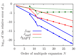
Figure 1: (Color online) Convergence of the $j_{0}$ term of the asymptotic expansion of $J(R)$ obtained when the multipole expansion of the primitive function is used in the variational, surface-integral, or SAPT formulas. Lines with squares indicate values obtained from eight-term Levin-$u$ extrapolation.

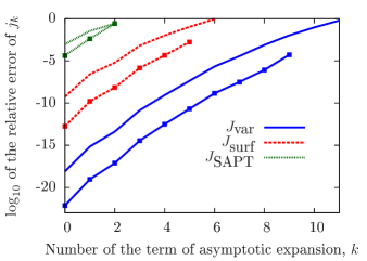
Figure 2: (Color online) Accuracy of the $j_{k}$ coefficients in the asymptotic expansion of $J(R)$ calculated using different exchange energy formulas and the multipole expansion of the primitive function, Eq. (2), summed through $N$=30. Lines with squares indicate values obtained from eight-term Levin-$u$ extrapolation.

The regular convergence with respect to $N$ occurs not only for $j_{0}$ but also for higher coefficients, allowing for successful extrapolation. Figure 2 presents the decimal logarithms of relative errors of $j_{k}$’s calculated with the three exchange energy formulas investigated in our work. This graph shows the accuracy of the raw results obtained for $N=30$ and the very significant gain in accuracy due to the Levin extrapolation. Note that in Fig. 2 we did not show the results of Levin’s $u$-transform for $j_{6}^{\textrm{surf}}$, $j_{10}^{\textrm{var}}$, and $j_{11}^{\textrm{var}}$, as in these cases extrapolation cannot increase accuracy. This is because the $N=30$ terms are not sufficient to establish the regularity of convergence. Nevertheless, it can be concluded that Levin’s $u$-transform is efficient at accelerating the convergence of the series investigated in our work, provided adequately large $N$ is used.

III.2 Exchange splitting from the multipole expansion of the first-order polarization function

In practice, the simplest nontrivial approximation to the primitive function $\varphi$ is provided by the first-order polarization function $\Phi^{(1)}=\varphi_{0}+\varphi^{(1)}$, defined in Sec. II.3. In the present subsection we shall find out how accurate values of $j_{0}$ can be obtained from the multipole expansion of $\varphi^{(1)}$, given by Eq. (24).

The value of $j_{0}^{\textrm{SAPT}}[\Phi^{(1)}_{N}]$ has been already given in the literature Chalasinski:73b . Using our notation the result of Ref. Chalasinski:73b, can be restated as follows

$$\frac{2}{e}j_{0}^{\textrm{SAPT}}[\Phi^{(1)}_{N}]=-\frac{2}{3}-\sum_{n=2}^{N}\frac{4}{n(n+1)(n+2)(n+3)}.$$ (51)

The inverse d’Alembert ratio of the series on the r.h.s. of Eq. (51) is equal to $1+4\,n^{-1}+O(n^{-2})$ so its convergence radius is equal to 1, i.e., is the same as for the series of Eq. (38). It is disappointing that the series of Eq. (38), obtained with the function $\Phi_{N}$, exhibit somewhat poorer convergence rate that the series of Eq. (51), obtained with the first-order approximation $\Phi^{(1)}_{N}$ to $\Phi_{N}$ . Taking into account that the sum of the series in Eq. (51) equals $-1/18$, we find that $j_{0}^{\textrm{SAPT}}[\Phi^{(1)}]=-13e/36$, which differs from the exact value by $-$1.8%. This result has been obtained using different method (without the multipole expansion) in Ref. Chalasinski:73a, .

The expression for $j_{\textrm{surf}}[\Phi^{(1)}_{N}]$ can be deduced from the results of Tang et al.Tang:91 Equation (7.25) of that work implies that

$$\frac{2}{e}j_{0}^{\textrm{surf}}[\Phi^{(1)}_{N}]=-\frac{1}{2}\bigg{(}1+\sum_{n=2}^{N}\frac{1}{n\,2^{n}}\bigg{)}^{2}.$$ (52)

One can easily find that the increment ratio for the sequence $j_{0}^{\textrm{surf}}[\Phi^{(1)}_{N}]$ equals $2+2\,N^{-1}+O(N^{-2})$, so the corresponding convergence radius is equal 2. The $N\rightarrow\infty$ limit of the r.h.s. of Eq. (52) is $-\frac{1}{2}\left(\ln 2+\frac{1}{2}\right)^{2}$, and the corresponding approximate value of $j_{0}$, given by $j_{0}^{\textrm{surf}}[\Phi^{(1)}_{N}]$, differs by $-$3.3% from the exact value $j_{0}=-1$. Thus, the first-order polarization function gives a better approximation to the exchange splitting when used in the SAPT formula than in the surface-integral formula.

The evaluation of $j_{0}^{\textrm{var}}[\Phi^{(1)}_{N}]$ is somewhat more complicated. Using the large-$R$ asymptotic estimation of the integral

$$\frac{1}{\pi}\int e^{-r_{a}-r_{b}}r_{a}^{k}r_{b}^{l}P_{m}(\cos\theta_{a})P_{n}(\cos\theta_{b})d^{3}{\bf r}=$$ (53)

$$\quad=2e^{-R}\frac{(k+1)!(l+1)!}{(k+l+3)!}[R^{k+l+2}+O(R^{k+l+1})]$$

one can find that

$$\frac{2}{e}j_{0}^{\textrm{var}}[\Phi^{(1)}_{N}]=-\frac{2}{3}-\sum_{k=2}^{N}\frac{8}{k(k+1)(k+2)(k+3)}$$ (54)

$$+2\sum_{k,l=2}^{N}\frac{(k-1)!(l-1)![kl(k+l+4)-2]}{(k+l+3)!}.$$

The double sum in Eq. (54) and its $N\rightarrow\infty$ limit can be worked out analytically and one obtains

$$\frac{2}{e}\lim_{N\rightarrow\infty}j_{0}^{\textrm{var}}[\Phi^{(1)}_{N}]=-\frac{989}{540}+\frac{\pi^{2}}{9}.$$ (55)

The resulting approximate value of $j_{0}$ differs from the exact one by only 0.12%. It may be noted that the value of $j_{0}^{\textrm{var}}[\Phi^{(1)}]$, equivalent to Eq. (55), has been obtained earlier by Chipman and Hirschfelder Chipman:73 without the help of the multipole expansion using the closed-form expression for $\varphi^{(1)}$.

The $N$ convergence of the sequence on the r.h.s. of Eq. (54) turns out to be rather slow. One can show analytically that the ratio of the $N$th and the $(N+1)$th increments, defined as in Eq. (45) with $\Phi_{N}$ replaced by $\Phi^{(1)}_{N}$ and denoted by $\rho^{(1)}_{N}(j_{0}^{\textrm{var}})$, behaves at large $N$ as

$$\rho^{(1)}_{N}(j_{0}^{\textrm{var}})=1+6\,N^{-1}+O(N^{-2}).$$ (56)

Thus, the sequence $j_{0}^{\textrm{var}}[\Phi^{(1)}_{N}]$ converges at large $N$ as a series with the convergence radius equal to 1. This seems to be in a disagreement with Eq. (46), which may suggest a faster convergence. It turns out, however, that when the multipole expansion of the higher polarization functions $\Phi^{(K)}_{N}$ is used, the $N$-convergence of $j_{0}^{\textrm{var}}[\Phi^{(K)}_{N}]$ corresponds also to the convergence radius 1. We have found by fitting the following large-$N$ behavior of $\rho^{(K)}_{N}(j_{0}^{\textrm{var}})$

$$\rho^{(K)}_{N} (j_{0}^{\textrm{var}})=1+(2K+4)\,N^{-1}$$ (57)

$$-(K-1)N^{-1}(\ln N)^{-1}+O\big{(}N^{-1}(\ln N)^{-2}\big{)}.$$

The prefactor $2K+4$ in the subleading term in Eq (57) shows that although the convergence radius for each $K$ is equal to 1, the rate of convergence improves with increasing $K$. This rate becomes geometric only in infinite order in $V$, i.e., at $K=\infty$, when Eq. (46) holds. However, we have noted in Sec. II.3 that $\Phi^{(K)}_{N}=\Phi_{N}$ when $N\leq 2K$. One can expect, then, that

$$\rho^{(K)}_{N}(j_{0}^{\textrm{var}})=\rho_{N}(j_{0}^{\textrm{var}})=4-2\,N^{-1}+O(N^{-2}),$$ (58)

in the range of $N$ values smaller or equal to 2$K$. Thus, $\rho^{(K)}_{N}(j_{0}^{\textrm{var}})$ is given by Eq. (57) at $N\!\gg\!2K$ and by Eq (57) at $N\leq 2K$. This is indeed the case as shown in Fig. 3, where the increment rations $\rho^{(K)}_{N}(j_{0}^{\textrm{var}})$ are presented for $K$=40 and $K$=80. The switch from the fast geometric convergence at low $N$ to the slow harmonic convergence at high $N$ is well seen. One can showGniewek:15 that this switch occurs at $N\approx N_{c}$, where $N_{c}$ is the solution of a transcendental equation

$$\frac{\Gamma(N_{c}+1)\Gamma(N_{c}+2K+6)}{\Gamma(2N_{c}+3)}=2e\frac{(2K+2)!}{2^{K}K!}.$$ (59)

This equation correctly describes the behavior of $\rho_{N}^{(K)}$, for instance for $K=40$ and $K=80$ it gives $N_{c}=232.3$ and $K=80$ $N_{c}=507.9$, respectively, in a good agreement with the values deduced from Fig. 3. The conclusion of the considerations in this subsection is that the inclusion of high-order effects in $V$ is necessary to obtain a fast converging approximation of the exchange splitting energy at large $R$.

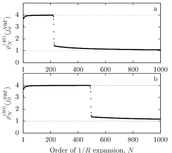
Figure 3: The increment rations $\rho^{(K)}_{N}(j_{0}^{\textrm{var}})$ for $K=40$ (panel a) and $K=80$ (panel b) as a function of $N$.

III.3 Exchange splitting from a variational approximation to the primitive function

The calculations of high-order multipole corrections may not be practical for many-electron systems, nevertheless we believe that the methods described above can be adapted for larger diatomics. This can be achieved via the use of Rayleigh-Ritz variational calculations of the primitive function with appropriately localized basis set, i.e., with trial functions satisfying the localization condition of Eq. (13). In order to test the effectiveness of this approach we applied the basis set employed in our previous work on the same system Gniewek:14 , but restricted to orbitals centered exclusively at the nucleus $a$. This restriction makes the basis set orthogonal for any $R$. The parameter $\Omega$ employed in Ref. Gniewek:14, to control the size of the basis set (defined as the maximal sum of the order of the included Laguerre and Legendre polynomials) is closely connected to the extent of the multipole expansion of $\varphi$ that can be recovered by the variational calculation. For example $\varphi_{N}$ can be recovered with the $\Omega=N$, but not with the $\Omega=N-1$ basis set. We performed variational calculations of $\varphi$ for 46 internuclear distances $R$=60, 62,…,150, followed by the application of the exchange energy formulas $J_{\textrm{SAPT}}[\varphi]$, $J_{\textrm{surf}}[\varphi]$ and $J_{\textrm{var}}[\varphi]$ and least-squares fitting of the obtained values of $J(R)$ to extract the constants $j_{0}$, $j_{1}$ and $j_{2}$. The results of these calculations for $\Omega=10$ are given in Table 5 together with the values obtained with the function $\Phi_{10}$, which are given for comparison. It is seen that the agreement of the $j_{0}$ values calculated with the multipole expansion and with the variational approximation to $\varphi$ is excellent. In the case of the higher constants $j_{1}$ and $j_{2}$ the agreement is not so good but reasonable, the multipole expansion giving consistently better results. As expected the volume-integral formula of Eq. (7) performs best not only in the case of the multipole expansion of the primitive function, but also with the variational approximation to this function.

Table 5: Values of $j_{0}$, $j_{1}$ and $j_{2}$ evaluated using the surface- and volume-integral formulas and the primitive function approximated using either the multipole expansion through the $10$th order ($\Phi_{10}$), or the variational treatment with localized, $\Omega=10$ basis ($\Phi^{V\!L\!B}_{10}$).

method	$j_{0}$	$j_{1}$	$j_{2}$
$J_{\textrm{SAPT}}[\Phi_{10}]$	$-0.9935\ 8974$	$-0.444\ 639$	$2.2909$
$J_{\textrm{SAPT}}[\Phi^{V\!L\!B}_{10}]$	$-0.9935\ 8952$	$-0.490\ 467$	$1.8381$
$J_{\textrm{surf}}[\Phi_{10}]$	$-0.9994\ 0777$	$-0.515\ 396$	$3.3341$
$J_{\textrm{surf}}[\Phi^{V\!L\!B}_{10}]$	$-0.9994\ 0757$	$-0.538\ 712$	$3.8320$
$J_{\textrm{var}}[\Phi_{10}]$	$-0.9999\ 9946$	$-0.500\ 022$	$3.1260$
$J_{\textrm{var}}[\Phi^{V\!L\!B}_{10}]$	$-0.9999\ 9965$	$-0.499\ 994$	$3.1185$
exact	$-1.0$	$-0.5$	$3.125$

IV Summary and Conclusions

Tang et al.Tang:91 showed that leading constant $j_{0}$ in the asymptotic expansion of the exchange splitting $J(R)=2e^{-R-1}R(j_{0}+j_{1}R^{-1}+j_{2}R^{-2}+\cdots)$ for H${}^{+}_{2}$ can be obtained when the surface-integral formula $J_{\textrm{surf}}[\varphi]$ of Eq. (5) is evaluated with the multipole expanded polarization series for the wave function. These authors inferred that the polarization series converges to the primitive function $\varphi$, rather than to the fully symmetric ground state function $\psi_{g}$, but his conclusion was later shown to be invalid, as Ćwiok et. al Cwiok:92:pol gave compelling evidence of the convergence to $\psi_{g}$.

Our work significantly extends the results of Tang et al.Tang:91 as we have calculated not only the leading but also higher terms in the asymptotic expansion of $J(R)$. We applied the surface-integral formula as well, but also two other exchange energy expressions that have not been previously considered in the present context: the volume-integral formula $J_{\textrm{SAPT}}[\varphi]$, Eq. (6), and the powerful volume-integral formula $J_{\textrm{var}}[\varphi]$ based on the Rayleigh-Ritz variational principle, Eq. (7). We have also calculated the convergence radii for the expansions resulting when of the constants $j_{0}$,$\ldots$,$j_{3}$ are calculated using the considered exchange energy expressions and the multipole expansion for the primitive function $\varphi$.

We found that the variational and surface-integral formulas lead to convergent expansions for the $j_{k}$ constants. The best convergence and the largest convergence radius, equal to 4, was found for the expansions obtained using the variational volume-integral formula. The convergence radius corresponding to the application of the surface-integral formula, $J_{\textrm{surf}}[\varphi]$, was found to be equal to 2. In the case of the SAPT formula, we found that the convergence for the constants $j_{0}$, $j_{1}$, and $j_{2}$ is slow with the convergence radius equal to 1. Moreover the expansion for $j_{2}$ converges to an incorrect value. The expansions for the higher constants $j_{k}$, $k>2$, generated by the SAPT formula turned out to be divergent.

When the multipole expansion for the first- or any finite-order polarization function is used to represent the primitive function $\varphi$, the resulting expansion for $j_{0}$ has convergence radius equal to one. Nevertheless the rate of convergence improves significantly with increasing order of the polarization expansion. This shows the importance of a high-order treatment in the interaction potential $V$ to obtain a good approximation for the $j_{0}$ constant. Our results do not contradict the convergence of the polarization expansion to the symmetric ground-state function $\psi_{g}$ (for which all three energy formulas are singular) but rely on the fact that the polarization expansion converges asymptotically to the primitive function $\varphi$.

Since the calculation of high-order multipole corrections for many-electron systems is not practical, we have presented an alternative method of obtaining the primitive function: variational calculation with appropriately localized basis set. We have shown that this variationally obtained primitive function provides excellent values of $j_{0}$ and reasonably good approximations to higher-order $j_{k}$ constants. Also in this case the variational volume formula provides the most accurate results.

Our study shows that the conventional SAPT formula exhibits some deficiencies for the calculation of the exchange energy at large interatomic distances of $R$. The variational volume formula leads to much faster convergence and significantly more accurate results when applied both with the multipole expansion of the wave function and with a suitable variational approximation to this function. Moreover this formula provides a much better basis set convergence of the results than the surface integral formula. One can therefore conclude that the variational volume-integral formula provides an attractive alternative for the determination of the exchange splitting and the exchange contribution of the interaction potential in general.

- (1) A. J. Stone, in The Theory of Intermolecular Forces (University Press, Oxford, 2013)
- (2) B. Jeziorski, R. Moszyński, and K. Szalewicz, Chem. Rev. 94, 1887 (1994)
- (3) R. Ahlrichs, Theor. Chim. Acta 41, 7 (1976)
- (4) J. D. Morgan III and B. Simon, Int. J. Quant. Chem. 17, 1143 (1980)
- (5) R. J. Damburg, R. Kh. Propin, S. Graffi, V. Grecchi, E. M. Harrell II, J. Čížek, J. Paldus, and H. J. Silverstone, Phys. Rev. Lett. 52, 1112 (1984)
- (6) J. Čížek, R. J. Damburg, S. Graffi, V. Grecchi, E. M. Harrell II, J. G. Harris, S. Nakai, J. Paldus, R. Kh. Propin, and H. J. Silverstone, Phys. Rev. A 33, 12 (1986)
- (7) S. Graffi, V. Grecchi, E. M. Harrell II, and H. J. Silverstone, Ann. Phys. (N.Y.) 165, 441 (1985)
- (8) R. H. Young, Int. J. Quant. Chem. 9, 47 (1975)
- (9) Y.-H. Zhang, L.-Y. Tang, X.-Z. Zhang, J. Jiang, and J. Mitroy, The Journal of Chemical Physics 136, 174107 (2012)
- (10) G. Jansen, Theor. Chem. Acc. 104, 499 (2000)
- (11) D. J. Klein, Int. J. Quant. Chem. 32, 377 (1987)
- (12) W. Kutzelnigg, J. Chem. Phys. 73, 343 (1980)
- (13) K. Szalewicz, K. Patkowski, and B. Jeziorski, in Intermolecular Forces and Clusters (Structure and Bonding, volume 116), edited by D. J. Wales (Springer-Verlag, Heidelberg, 2005) pp. 43–117
- (14) C. Herring, Rev. Mod. Phys. 34, 631 (1962)
- (15) V. Galitski, E. Nikitin, and B. Smirnov, Teoria stolknovenii atomnykh chastic (Collision theory of atomic particles) (Nauka, Moscow, 1981)
- (16) B. M. Smirnov, Physics-Uspekhi 44, 221 (2001)
- (17) O. B. Firsov, Zh. Exp. Theor. Fiz 21, 1001 (1951)
- (18) T. Holstein, J. Phys. Chem. 56, 832 (1952)
- (19) L. P. Gor’kov and L. P. Pitaevskii, Sov. Phys. Dokl. 8, 788 (1964)
- (20) C. Herring and M. Flicker, Phys. Rev. 134, A362 (1964)
- (21) B. L. Burrows, A. Dalgarno, and M. Cohen, Phys. Rev. A 86, 052525 (2012)
- (22) B. M. Smirnov and M. I. Chibisov, Sov. Phys. JETP 21, 624 (1965)
- (23) J. N. Bardsley, T. Holstein, B. R. Junker, and Swati Sinha, Phys. Rev. A 11, 1911 (1975)
- (24) K. T. Tang, J. P. Toennies, M. Wanschura, and C. L. Yiu, Phys. Rev. A 46, 3746 (1992)
- (25) T. C. Scott, M. Aubert-Frécon, and D. Andrae, Applicable Algebra in Engineering, Communication and Computing 13, 233 (2002)
- (26) T. C. Scott, M. Aubert-Frécon, G. Hadinger, D. Andrae, J. Grotendorst, and J. D. Morgan III, J. Phys. B 37, 4451 (2004)
- (27) M. J. Jamieson, A. Dalgarno, M. Aymar, and J. Tharamel, J. Phys. B 42, 095203 (2009)
- (28) B. L. Burrows, A. Dalgarno, and M. Cohen, Phys. Rev. A 81, 042508 (2010)
- (29) U. Kleinekathöfer, K. Tang, J. Toennies, and C. Yiu, Chemical Physics Letters 249, 257 (1996)
- (30) U. Kleinekathöfer, Chemical Physics Letters 324, 403 (2000)
- (31) T. Scott, M. Aubert-Frécon, D. Andrae, J. Grotendorst, J. M. III, and M. Glasser, Applicable Algebra in Engineering, Communication and Computing 15, 101 (2004)
- (32) C. L. Yiu, K. T. Tang, and W. G. Greenwood, The Journal of Physical Chemistry A 115, 7346 (2011)
- (33) Y. M. Chen, X. Y. Kuang, X. W. Sheng, and X. Z. Yan, The Journal of Physical Chemistry A 118, 592 (2014)
- (34) T. C. Scott, A. Dalgarno, and J. D. Morgan III, Phys. Rev. Lett. 67, 1419 (1991)
- (35) M. V. Khoma, O. M. Karbovanets, M. I. Karbovanets, and R. J. Buenker, Physica Scripta 78, 065201 (2008)
- (36) M. I. Chibisov and R. K. Janev, Phys. Rep. 166, 1 (1988)
- (37) P. Gniewek and B. Jeziorski, Phys. Rev. A 90, 022506 (2014)
- (38) B. Jeziorski, K. Szalewicz, and G. Chałasiński, Int. J. Quant. Chem. 14, 271 (1978)
- (39) K. Szalewicz, WIREs: Comput. Mol. Sci. 2, 254 (2012)
- (40) E. G. Hochenstein and C. D. Sherrill, WIREs: Comput. Mol. Sci. 2, 127304 (2012)
- (41) G. Jansen, WIREs: Comput. Mol. Sci. 4, 127 (2014)
- (42) A. Hesselmann and T. Korona, J. Chem. Phys. 141, 094107 (2014)
- (43) R. K. Janev and L. Presnyakov, Phys. Rep. 70, 1 (1981)
- (44) E. M. Harrell, Commun. Math. Phys. 75, 239 (1980)
- (45) A. A. Ovchinnikov and A. D. Sukhanov, Sov. Phys. Dokl. 9, 685 (1965)
- (46) I. V. Komarov and S. Yu. Slavyanov, Sov. Phys. JETP 25, 910 (1967)
- (47) R. J. Damburg and R. Kh. Propin, J. Phys. B 1, 681 (1968)
- (48) K. T. Tang, J. P. Toennies, and C. L. Yiu, J. Chem. Phys. 94, 7266 (1991)
- (49) J. O. Hirschfelder, Chem. Phys. Lett. 1, 325 (1967)
- (50) E. Brezin and J. Zinn-Justin, J. Physique Lett. 40, 511 (1979)
- (51) J. Čížek, J. M. Clay, and J. Paldus, Phys. Rev. A 22, 793 (1980)
- (52) A. Dalgarno and N. Lynn, Proc. Phys. Soc. Lonon. 70, 223 (1957)
- (53) G. Chałasiński, B. Jeziorski, and K. Szalewicz, Int. J. Quant. Chem. 11, 247 (1977)
- (54) K. T. Tang, J. P. Toennies, C. L. Yiu, T. Ćwiok, B. Jeziorski, W. Kolos, and R. Moszyński, Chem. Phys. Lett. 224, 476 (1994)
- (55) T. Ćwiok, B. Jeziorski, W. Kołos, R. Moszyński, J. Rychlewski, and K. Szalewicz, Chem. Phys. Lett. 195, 67 (1992)
- (56) W. Kutzelnigg, Chem. Phys. Lett. 195, 77 (1992)
- (57) B. Jeziorski and W. Kołos, in Molecular interactions, Vol. 3, edited by H. Ratajczak and W. J. Orville-Thomas (Wiley, New York, 1982) pp. 1–46
- (58) A. Dalgarno and J. T. Lewis, Proc. Roy. Soc. A 233, 70 (1955)
- (59) P. Gniewek and B. Jeziorski, unpublished results (2015)
- (60) G. B. Arfken, Mathematical methods for physicists (Academic Press, New York, 1968)
- (61) D. Levin, Int. J. Comput. Math. 3, 371 (1972)
- (62) E. J. Weniger, Comput. Phys. Rep. 10, 189 (1989)
- (63) G. Chałasiński and B. Jeziorski, Int. J. Quant. Chem. 7, 745 (1973)
- (64) G. Chałasiński and B. Jeziorski, Int. J. Quant. Chem. 7, 63 (1973)
- (65) D. M. Chipman and J. O. Hirschfelder, J. Chem. Phys. 59, 2838 (1973)