Refraction in planetary atmospheres: improved analytical expressions and comparison with a new ray tracing algorithm

Abstract

Atmospheric refraction affects to various degrees exoplanet transit, lunar eclipse, as well as stellar occultation observations. Exoplanet retrieval algorithms often use analytical expressions for the column abundance along a ray traversing the atmosphere as well as for the deflection of that ray, which are first order approximations valid for low densities in a spherically symmetric homogeneous isothermal atmosphere. We derive new analytical formulae for both of these quantities, which are valid for higher densities, and use them to refine and validate a new ray tracing algorithm which can be used for arbitrary atmospheric temperature-pressure profiles. We illustrate with simple isothermal atmospheric profiles the consequences of our model for different planets: temperate Earth-like and Jovian-like planets, as well as HD189733b, and GJ1214b. We find that, for both hot exoplanets, our treatment of refraction does not make much of a difference to pressures as high as 10 atmosphere, but that it is important to consider the variation of gravity with altitude for GJ1214b. However, we find that the temperate atmospheres have an apparent scale height significantly smaller than their actual density scale height at densities larger than 1 amagat, thus increasing the difficulty of detecting spectral features originating in these regions. These denser atmospheric regions form a refractive boundary layer where column abundances and ray deflection increases dramatically with decreasing impact parameter. This refractive boundary layer mimics a surface, and none of the techniques mentioned above can probe atmospheric regions denser than about 4 amagat on these temperate planets.

1 Introduction

Most analytical expressions of an exoplanetary primary transit lightcurve are derived from analytical expressions of the optical depth along an unrefracted ray, i.e. that travels in a straight light, through a homogeneous isothermal atmospheres (see e. g. Fortney 2005; Lecavelier des Etangs et al. 2008; Benneke & Seager 2012; Howe & Burrows 2012; de Wit & Seager 2013; Griffith 2014). However, several papers (Hui & Seager 2002; Sidis & Sari 2010; García Muñoz et al. 2012; Bétrémieux & Kaltenegger 2013, 2014; Misra, Meadows & Crisp 2014; Misra & Meadows 2014) have emphasised the importance of the refractive bending of light by exoplanetary atmospheres on these lightcurves. Refraction is also important in various observational geometries in our Solar System. It influences the perceived brightness of a star during a stellar occultation by a planetary atmosphere (see the review by Smith & Hunten 1990) which can then be used to infer the planet’s atmospheric composition. It also determines the brightness of moons eclipsed by their parent planet. Indeed, as a moon moves deeper in the penumbra, solar radiation must traverse deeper atmospheric regions of the eclipsing planet in order to be bent sufficiently to reach the moon. Several Lunar eclipse observations were analysed to derive the transmission of Earth’s atmosphere (Pallé et al. 2009; Vidal-Madjar et al. 2010; García Muñoz et al. 2012, Arnold et al. 2014) using this principle.

Given the importance of atmospheric refraction in these various observational geometries, it is worthwhile to have analytical formulae which include refraction, both to compute the ray’s deflection, as well as the integrated number density along the deflected ray, or its column abundance. Combined with an atmosphere-averaged extinction cross section, one can compute the optical depth along the ray, and the corresponding atmospheric transmission with Beer’s law. However, computing the column abundance and the deflection requires solving complicated integrals for which analytical expressions exist only under simplifying assumptions. In section 2, we derive analytical solutions of these integrals by expanding the integrand in a Taylor-series up to the second order with respect to refractivity, and then evaluate the integral for each of these terms. This is done for a homogeneous isothermal atmosphere, since this is the level of complexity considered by some exoplanet atmosphere retrieval algorithm (see e.g. Charbonneau et al. 2009; Howe & Burrows 2012; Anglada-Escudé et al. 2013; Ehrenreich et al. 2014; Waldmann et al. 2014). We also derive an order-of-magnitude estimate of the sum of the remaining uncomputed higher-order terms in the Taylor series, in order to determine the density region over which our analytical expressions are useful.

Since planetary atmospheres are usually not isothermal, we have to rely on numerical methods to deal with these general cases for which analytical solutions do not exist. In section 3, we describe MAKEXOSHELL, a new numerical ray tracing algorithm that computes the column abundance and the deflection for rays traversing a spherically symmetric atmosphere given an arbitrary one-dimensional (1-D) temperature-pressure profile as input. We also describe how we compute the model atmosphere, as well as its refractivity, which are inputs to MAKEXOSHELL. In section 4, we compare the output of the numerical algorithm with our analytical expressions for an Earth-like planet with a homogeneous isothermal atmosphere, in order to mutually validate both methods. We also discuss the impact of our new model on temperate Earth-like and Jovian-like exoplanets, as well as for two already well-observed exoplanets: HD189733b and GJ1214b. We summarise our results in section 5.

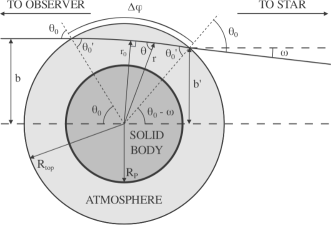
Figure 1: Trajectory through a planetary atmosphere of an observed light ray during an exoplanetary primary transit. The solid body, or opaque region, of the planet (dark grey) and its atmosphere (light grey) are shown, along with the axis running from the observer to the centre of the planet (dashed line) with the observer to the left and the star to the right. The radius of the planetary surface, $R_{p}$, and of the top of the atmosphere, $R_{top}$, as well as the zenith angle, $\theta$, of the ray for a given height, r, are also indicated. A light ray observed with an impact parameter $b$, entered the atmosphere with an incidence angle $\theta_{0}$ a projected distance $b^{\prime}$ to the centre of the planet with respect to the observer, reached a grazing height $r_{0}$, and is deflected by $\omega$ by the atmosphere.

2 Analytical expressions

2.1 Basic equations

As light rays traverse a planetary atmosphere, they are bent by refraction toward the surface of the planet (see Fig. 1) due to the exponential increase of atmospheric refractivity (the refraction index minus one), with decreasing altitude. The trajectory of a ray is described by an invariant, $b$, which is equal to its impact parameter (Phinney & Anderson 1968; Bétrémieux & Kaltenegger 2013, 2014)

$$b=r(1+\nu)\sin{\theta}=r_{0}(1+\nu_{0})=R_{top}\sin{\theta_{0}}.$$ (1)

Here, $r$ is the radial position with respect to the centre of the planet (i.e. radius + altitude), which for the sake of brevity we will refer to as height throughout the paper, while $\nu$ and $\theta$ are the refractivity of the atmosphere and the zenith angle of the ray at that height, respectively. $r_{0}$ is the minimum height reached by a ray, or its grazing height, where the atmospheric refractivity is $\nu_{0}$. $R_{top}$ is the radial position of the top of the atmosphere and $\theta_{0}$ is the zenith angle of the ray at the top of the atmosphere, or simply its incidence angle. The atmosphere deflected the ray by $\omega$, and the ray entered the atmosphere a projected distance $b^{\prime}$ to the centre of the planet, with respect to the observer, given by

$$b^{\prime}=\left(\frac{\sin(\theta_{0}-\omega)}{\sin{\theta_{0}}}\right)b.$$ (2)

The change in zenith angle of the ray with height is given by,

$$\frac{d\theta}{dr}=-\frac{\tan{\theta}}{(1+\nu)}\left(\frac{d\nu}{dr}\right)-\frac{\tan\theta}{r}.$$ (3)

The first term is the refractive term and comes from Snell’s law. The second term is the geometric term, and comes from the equation of an unrefracted ray, $b=r\sin\theta$, which proceeds in a straight line. Note that all of the equations involving angles are valid when these are expressed in radians, even though in section 4 we quote results in degrees.

The atmospheric refractivity is given by,

$$\nu=\left(\frac{n}{n_{STP}}\right)\sum_{j}f_{j}{\nu_{STP}}_{j}=\left(\frac{n}{n_{STP}}\right)\nu_{STP},$$ (4)

where $n$ is the number density, $n_{STP}$ is the number density at standard temperature and pressure (STP) also known as Loschmidt’s number, $f_{j}$ is the mole fraction of the j^th chemical species, ${\nu_{STP}}_{j}$ is the STP refractivity of the j^th species, while $\nu_{STP}$ is the STP refractivity of the atmosphere. The ratio inside the parenthesis in equation 4 is the number density expressed in units of amagat. Note that the STP refractivity is simply the refractivity for a density of 1 amagat, which can be achieved for temperatures other than 273.15 K with the appropriate pressure.

The number density, $n$, in an atmospheric region varies with height, and this dependence can be expressed by

$$n_{U}=n_{L}e^{-(r_{U}-r_{L})/H},$$ (5)

so that

$$\frac{dn}{dr}=-\frac{n}{H},$$ (6)

where $H$ is the density scale height in that atmospheric region, and the $U$ and $L$ subscripts denote quantities for the upper and lower boundaries of the region, respectively. Thus,

$$\frac{d\nu}{dr}=\frac{\nu_{STP}}{n_{STP}}\left(\frac{dn}{dr}\right)=-\left(\frac{n}{n_{STP}}\right)\frac{\nu_{STP}}{H}=-\frac{\nu}{H}.$$ (7)

Note that this result holds only for a homogeneous atmospheric region where the composition of the major constituents that contribute significantly to the refraction index does not change with height, i.e. that $\nu_{STP}$ is constant with height. This assumption will be carried throughout all derivations.

2.2 Lower atmospheric boundary

In order for a ray to traverse the atmosphere, $\theta$ must increase as $r$ decreases (or $d\theta$/$dr<0$) so that a downward-going ray reaches a minimum height, $r_{0}$, where it grazes the atmosphere ($\theta=\pi/2$). If $d\theta$/$dr>0$, the ray will spiral deeper into the atmosphere until it is absorbed. Using equations 3, we can derive that

$$-\frac{r}{(1+\nu)}\left(\frac{d\nu}{dr}\right)<1$$ (8)

is the necessary condition for a ray to traverse the atmosphere. Using equation 7, this can be rewritten as,

$$\left(\frac{\nu}{1+\nu}\right)\frac{r}{H}<1.$$ (9)

In the special case when this expression is equal to one, a ray which is tangential to the atmosphere will circle the planet as its radius of curvature matches its height. Knowing the height-dependence of the density, and thus refractivity, this equation can be solved recursively for this special height. As a ray approaches this height, both the column abundance and the deflection tend toward infinity. Atmospheric regions below this height cannot be probed by transmitted stellar radiation under any circumstance during a stellar occultation or an exoplanet primary transit. This is true only for a perfectly spherical planet free of horizontal density gradients (i.e. no weather or turbulence). Departure from these assumptions creates a diffuse boundary about which a grazing ray can or cannot escape the planet depending on local conditions. Furthermore, since refractivities vary with wavelength, so does the height of this lower boundary.

This lower boundary is always located below the critical altitude, described in Bétrémieux & Kaltenegger (2014), below which atmospheric regions cannot be probed by transmission spectroscopy when an exoplanet occults the central area of its host star. This critical altitude occurs where a ray, that comes from the opposite limb of the star, reaches an atmospheric critical density which causes it to be deflected by a critical deflection, $\omega_{c}$, toward the observer. During the course of the transit, the symmetry is broken and part of the planetary limb can be probed to lower altitudes while the opposite limb’s observable region is restricted to higher altitudes. However, the lowest altitude that one can probe only asymptotically approaches the lower boundary determined by equation 9, so that this boundary is the deepest atmospheric region that can ever be probed by exoplanet transmission spectroscopy or by stellar occultation.

2.3 Column abundance and ray deflection integrals

The column abundance, $N$, along a refracted ray, as well as its deflection, $\omega$, can be computed from

$$N=2\int_{r_{0}}^{\infty}dN\equiv 2\int_{r_{0}}^{\infty}F_{1}dr$$ (10)

and

$$\omega=2\int_{r_{0}}^{\infty}d\omega\equiv 2\int_{r_{0}}^{\infty}F_{2}dr$$ (11)

where the factor of 2 comes from a ray traversing an altitude region twice. Note that we have labelled the integrands in terms of the integration parameter $r$ in both equations for future use (see section 2.4).

The incremental column abundance, $dN$, of a ray is given by,

$$dN=\frac{n}{\cos{\theta}}dr.$$ (12)

The incremental deflection of a ray (expressed in radians), $dw$, is simply the first term in equation 3 (see also Goldsmith 1963; Auer & Standish 2000), which we rewrite as

$$d\omega=-\frac{\tan\theta}{(1+\nu)}\left(\frac{d\nu}{dr}\right)dr=\left(\frac{\nu}{1+\nu}\right)\frac{\tan\theta}{H}dr$$ (13)

for a homogeneous planetary atmosphere.

The trigonometric functions can be rewritten entirely in terms of $r$ and $\nu$. From equation 1, we have

$$\sin\theta=\frac{b}{r(1+\nu)}=\frac{r_{0}(1+\nu_{0})}{r(1+\nu)},$$ (14)

$$\frac{1}{\cos\theta}=\frac{1}{\sqrt{1-\sin^{2}\theta}}=\left(1-\left(\frac{r_{0}(1+\nu_{0})}{r(1+\nu)}\right)^{2}\right)^{-1/2},$$ (15)

and

$$\tan\theta=\frac{\sin\theta}{\cos\theta}=\left(\left(\frac{r(1+\nu)}{r_{0}(1+\nu_{0})}\right)^{2}-1\right)^{-1/2}.$$ (16)

Equations 10 and 11 are then given, for a homogeneous atmosphere, by

$$N=2\int_{r_{0}}^{\infty}n\left(1-\left(\frac{r_{0}(1+\nu_{0})}{r(1+\nu)}\right)^{2}\right)^{-1/2}dr,$$ (17)

and

$$\omega=2\int_{r_{0}}^{\infty}\left(\frac{\nu}{1+\nu}\right)\frac{1}{H}\left(\left(\frac{r(1+\nu)}{r_{0}(1+\nu_{0})}\right)^{2}-1\right)^{-1/2}dr$$ (18)

where most of the height-dependence is buried inside the refractivity.

2.4 Taylor-series expansion of integrands

No analytical solutions exist for the complicated integrals in equations 17 and 18, even in the case of a homogeneous isothermal atmosphere. However, refractivities are typically small, on the order of $10^{-4}$ at STP, such that one can expand the integrand in both equations in Taylor series in $\nu_{0}$, prior to carrying-out the integration. We carry out this Taylor expansion for both integrands $F_{1}$ and $F_{2}$ to the second order such that

$$dN = dN_{0}+dN_{1}+dN_{2}+...$$

$$= F_{1}|_{\nu_{0}=0}+\nu_{0}\left(\frac{dF_{1}}{d\nu_{0}}\right)_{\nu_{0}=0}+\frac{\nu_{0}^{2}}{2}\left(\frac{d^{2}F_{1}}{d\nu_{0}^{2}}\right)_{\nu_{0}=0}+...,$$

and

$$d\omega = d\omega_{0}+d\omega_{1}+d\omega_{2}+...$$

$$= F_{2}|_{\nu_{0}=0}+\nu_{0}\left(\frac{dF_{2}}{d\nu_{0}}\right)_{\nu_{0}=0}+\frac{\nu_{0}^{2}}{2}\left(\frac{d^{2}F_{2}}{d\nu_{0}^{2}}\right)_{\nu_{0}=0}+....$$

For a homogeneous isothermal atmosphere, we have the additional relations,

$$n=n_{0}e^{-(r-r_{0})/H}$$ (21)

and

$$\nu=\nu_{0}e^{-(r-r_{0})/H}$$ (22)

where $n_{0}$ and $\nu_{0}$ are the number density and the refractivity at a ray’s grazing height, respectively. The derivation of the various Taylor expansion terms is rather tedious and lengthy, so we will here only quote the results:

$$F_{1}|_{\nu_{0}=0}=\frac{n}{\sqrt{1-(r_{0}/r)^{2}}}=\frac{n(r/r_{0})}{\sqrt{(r/r_{0})^{2}-1}}$$ (23)

$$\left(\frac{dF_{1}}{d\nu_{0}}\right)_{\nu_{0}=0}=\frac{n(r/r_{0})(1-e^{-(r-r_{0})/H})}{[(r/r_{0})^{2}-1]^{3/2}}$$ (24)

$$\left(\frac{d^{2}F_{1}}{d\nu_{0}^{2}}\right)_{\nu_{0}=0}=\frac{3n(r/r_{0})^{3}(1-e^{-(r-r_{0})/H})^{2}}{[(r/r_{0})^{2}-1]^{5/2}}\\ -\frac{2n(r/r_{0})(1-e^{-(r-r_{0})/H})}{[(r/r_{0})^{2}-1]^{3/2}}$$ (25)

and,

$$F_{2}|_{\nu_{0}=0}=0$$ (26)

$$\left(\frac{dF_{2}}{d\nu_{0}}\right)_{\nu_{0}=0}=\frac{1}{H}\frac{e^{-(r-r_{0})/H}}{\sqrt{(r/r_{0})^{2}-1}}$$ (27)

$$\left(\frac{d^{2}F_{2}}{d\nu_{0}^{2}}\right)_{\nu_{0}=0}=\frac{2}{H}\frac{e^{-(r-r_{0})/H}}{\sqrt{(r/r_{0})^{2}-1}}\times\\ \left[\frac{(r/r_{0})^{2}(1-e^{-(r-r_{0})/H})}{(r/r_{0})^{2}-1}-e^{-(r-r_{0})/H}\right].$$ (28)

2.5 “Modified Bessel functions” solution

At first glance, it seems that we have made the problem more complicated as we have transformed each of our initial integrals into sums of three integrals, each of which also seem impossible to solve. However, a suggestion of a solution appears when one considers the modified Bessel functions of the second kind (Arfken, 1985),

$$K_{t}(z)=\frac{\pi^{1/2}}{(t-1/2)!}\left(\frac{z}{2}\right)^{t}\int_{1}^{\infty}e^{-zx}(x^{2}-1)^{t-1/2}dx$$ (29)

of which the first two functions are

$$K_{0}(z)=\int_{1}^{\infty}e^{-zx}(x^{2}-1)^{-1/2}dx,$$ (30)

and

$$K_{1}(z)=z\int_{1}^{\infty}e^{-zx}(x^{2}-1)^{1/2}dx,$$ (31)

which were derived from equation 29, knowing that $(-1/2)!=\pi^{1/2}$.

Consider, as a first step, the zeroth term in the column abundance integral,

$$N_{0} = 2\int_{r_{0}}^{\infty}dN_{0}=2\int_{r_{0}}^{\infty}\frac{n(r/r_{0})}{\sqrt{(r/r_{0})^{2}-1}}dr$$ (32)

$$= 2\int_{r_{0}}^{\infty}\frac{n_{0}(r/r_{0})e^{-(r-r_{0})/H}}{\sqrt{(r/r_{0})^{2}-1}}dr.$$

With the change of variable, $x=r/r_{0}$, it becomes

$$N_{0}=2n_{0}r_{0}e^{r_{0}/H}\int_{1}^{\infty}\frac{xe^{-(r_{0}/H)x}}{(x^{2}-1)^{1/2}}dx$$ (33)

which can be integrated by parts to yield

$$N_{0}=\left[2n_{0}r_{0}e^{r_{0}/H}(x^{2}-1)^{1/2}e^{-(r_{0}/H)x}\right]_{1}^{\infty}\\ +2n_{0}r_{0}e^{r_{0}/H}(r_{0}/H)\int_{1}^{\infty}e^{-(r_{0}/H)x}(x^{2}-1)^{1/2}dx.$$ (34)

The values of the first term at 1 and $\infty$ are both zero so the first term drops out. Whereas it is straightforward to derive for the value of 1, the $\infty$ case requires the use of l’Hôpital’s rule. The second term can be rewritten in terms of the modified Bessel functions of the second kind, so that we obtain

$$N_{0}=2n_{0}r_{0}e^{r_{0}/H}K_{1}(r_{0}/H)=2n_{0}r_{0}K_{1}^{*}(r_{0}/H)$$ (35)

where we adopt the following short-hand notation,

$$K_{t}^{*}(y)=e^{y}K_{t}(y)$$ (36)

for the remainder of this paper. This expression for the column abundance has been previously derived in terms of these modified Bessel functions (see e.g. Griffith 2014). However, this is only the leading term in our Taylor series, and corresponds to the non-refractive case.

Each of the terms in the column abundance and deflection expansion can also be rewritten in terms of these modified Bessel functions using the same change of variable, and then integrating by parts a number of times. At each integration by parts, we get a term that drops out when evaluated at 1 and $\infty$ and an integral term that can either be expressed as a modified Bessel function or must be further integrated by parts. Again, the derivation is straightforward but rather lengthy so we only here quote the results:

$$N_{1}=2n_{0}r_{0}\left(\frac{r_{0}\nu_{0}}{H}\right)\left[2K_{0}^{*}\left(\frac{2r_{0}}{H}\right)-K_{0}^{*}\left(\frac{r_{0}}{H}\right)\right]$$ (37)

$$N_{2}=n_{0}r_{0}\left(\frac{r_{0}\nu_{0}}{H}\right)^{2}\left[9K_{1}^{*}\left(\frac{3r_{0}}{H}\right)-8K_{1}^{*}\left(\frac{2r_{0}}{H}\right)+K_{1}^{*}\left(\frac{r_{0}}{H}\right)\right]\\ +n_{0}H\left(\frac{r_{0}\nu_{0}}{H}\right)^{2}\left[-7K_{0}^{*}\left(\frac{3r_{0}}{H}\right)+4K_{0}^{*}\left(\frac{2r_{0}}{H}\right)+K_{0}^{*}\left(\frac{r_{0}}{H}\right)\right]$$ (38)

and

$$\omega_{0}=0$$ (39)

$$\omega_{1}=2\left(\frac{r_{0}\nu_{0}}{H}\right)K_{0}^{*}\left(\frac{r_{0}}{H}\right)$$ (40)

$$\omega_{2}=2\left(\frac{r_{0}\nu_{0}}{H}\right)^{2}\left[2K_{1}^{*}\left(\frac{2r_{0}}{H}\right)-K_{1}^{*}\left(\frac{r_{0}}{H}\right)\right]\\ +2\left(\frac{r_{0}}{H}\right)\nu_{0}^{2}\left[-2K_{0}^{*}\left(\frac{2r_{0}}{H}\right)+K_{0}^{*}\left(\frac{r_{0}}{H}\right)\right].$$ (41)

Note that the leading term of the Taylor-series expansion for deflection, shown in equation 39, is 0 as expected since the leading term is the non-refractive case. Without refraction, light is not bent by the atmosphere.

2.6 “General power-series” solution

Expressions in power-series exists for these modified Bessel functions (Arfken, 1985), and are given by:

$$K_{t}^{*}(y)=\sqrt{\frac{\pi}{2y}}\left[1+\frac{(4t^{2}-1)}{8y}+\frac{(4t^{2}-1)(4t^{2}-9)}{128y^{2}}+...\right].$$ (42)

In our case, $y$ is always a multiple of $r_{0}/H$, which is always large. Thus, the second, third and higher-order terms in equation 42 decrease by successive powers of multiples of $r_{0}/H$, and are significantly smaller than the leading term in this series.

Collecting terms, equations 2.4 and 2.4 can be rewritten more generally as

$$N=\sqrt{\frac{2\pi r_{0}}{H}}(n_{0}H)\left[1+C_{0}+\sum_{j=1}^{\infty}C_{j}\left(\frac{r_{0}\nu_{0}}{H}\right)^{j}\right]$$ (43)

and

$$\omega=\sqrt{\frac{2\pi r_{0}}{H}}\nu_{0}\left[1+D_{0}+\sum_{j=1}^{\infty}D_{j}\left(\frac{r_{0}\nu_{0}}{H}\right)^{j}\right],$$ (44)

where $C_{j}$ and $D_{j}$ are coefficients for the column abundance and deflection, respectively. Even though we have only explicitly collected terms up to $j=2$ for the column abundance, and $j=1$ for the deflection, we can determine by inspection that higher-order terms follow this trend. These coefficients are themselves power-series expansion in term of $H/r_{0}$, but each of them quickly converges since this ratio is always small.

Both series depends on $\sqrt{2\pi r_{0}/H}$, the ratio of gas column abundance along a grazing ray to that along a vertical ray (given by $n_{0}H$) for a curved exponential atmosphere. This ratio, which we will call the slant factor, has been described before (see e.g. Fortney 2005). The leading non-zero term in both series matches previous expressions of the column abundance without refraction (see references listed in section 1), as well as first-order expressions for the ray deflection (Goldsmith 1963), respectively. Higher-order terms in the series are surprisingly dependent on powers of $(r_{0}\nu_{0}/H)$, and not simply $\nu_{0}$. Whereas $\nu_{0}$ is usually very small, it increases exponentially with depths so that combined with $r_{0}/H$, which is large, $(r_{0}\nu_{0}/H)$ can become of order unity. Hence, higher-order terms in the series are far from negligible when a ray travels deep enough in a planetary atmosphere. So over what range of densities can we use our analytical expressions?

We have only computed the coefficients up to the second order in refractivity as the length of the calculations, and correspondingly the odd of making a mathematical mistake, increases steeply with order. However, we can make an order-of-magnitude estimate of the sum of the terms for which we have not explicitly computed the $C_{j}$ and $D_{j}$ coefficients, for both the column abundance, $N_{rest}$, and the deflection, $\omega_{rest}$. This is done by assuming that the unknown coefficients are all identical to the highest-order computed coefficient. Under this crude assumption, we can write

$$N_{rest}=\sqrt{\frac{2\pi r_{0}}{H}}(n_{0}H)C_{2}\left(\frac{r_{0}\nu_{0}}{H}\right)^{3}\sum_{l=0}^{\infty}\left(\frac{r_{0}\nu_{0}}{H}\right)^{l}$$ (45)

and

$$\omega_{rest}=\sqrt{\frac{2\pi r_{0}}{H}}\nu_{0}D_{1}\left(\frac{r_{0}\nu_{0}}{H}\right)^{2}\sum_{l=0}^{\infty}\left(\frac{r_{0}\nu_{0}}{H}\right)^{l}$$ (46)

where the leading term for $C_{2}$ and $D_{1}$ are 0.27 and 0.41, respectively. The infinite sum, which appears in both equations 45 and 46, is a geometric series and converges to

$$\sum_{l=0}^{\infty}\left(\frac{r_{0}\nu_{0}}{H}\right)^{l}=\left(1-\frac{r_{0}\nu_{0}}{H}\right)^{-1}$$ (47)

but only when

$$\frac{r_{0}\nu_{0}}{H}<1.$$ (48)

It is interesting to note that the condition for the convergence of this series is very close to the condition for a ray to traverse the atmosphere, shown in equation 9. Indeed, they only differ by a factor $(1+\nu_{0})$ when evaluated at $r_{0}$. Since $(1+\nu_{0})\gtrsim 1$, equation 9 is automatically satisfied when equation 48 is satisfied. The fact that they are not exactly the same is probably due to our crude method of estimating the remaining terms.

3 Numerical model

3.1 Ray-tracing algorithm

We have made substantial improvements to an algorithm that, given a 1-D model atmospheric temperature-pressure altitude profile, traces rays through that atmosphere and computes the number density column abundance along the rays as well as their deflection by the atmosphere. This algorithm, which has been previously described by Bétrémieux & Kaltenegger (2013, 2014) and references therein, suffered from numerical instabilities in the computed ray deflection, which started at densities of about $5\times 10^{-5}$ amagat, and became worse with lower densities, such that the algorithm was useless for densities below $3\times 10^{-6}$ amagat. These numerical instabilities were not only due to improper treatment of integer to double precision conversion of variables, but also intrinsically due to the method. Indeed, we were computing the ray deflection by first computing the azimuthal travel of the ray through the atmosphere, $\Delta\phi$ (see Fig. 1), and then using

$$\omega=\Delta\phi+2\theta_{0}-\pi,$$ (49)

thus subtracting two large numbers from each other to get a much smaller quantity. We have modified the algorithm and reduced these numerical instabilities considerably. In this section, we will describe the new algorithm which we name MAKEXOSHELL.

The inputs to MAKEXOSHELL include a 1-D model atmosphere’s temperature and pressure, or $T$ and $P$, as a function of altitude, $z$. Also required are the radius of the planet, $R_{P}$, the highest and lowest altitudes of the computational region, the number of rays and layers sampling this altitude region, and the STP refractivity of the atmosphere. Given temperatures and pressures from the model atmosphere, typically in increments of 1 km altitude, MAKEXOSHELL uses the ideal gas law to determine the corresponding densities. This serves as a basis for the rest of the computation done on a much finer altitude grid, or computational grid.

MAKEXOSHELL assumes that the atmosphere within a model atmosphere layer follows an exponential behaviour with a constant density scale height as displayed in equation 5. Once the scale height within that layer is computed, using the densities at its upper and lower boundaries, densities are interpolated on the computational grid within that layer. Thus, MAKEXOSHELL builds-up a density profile on the computational grid from the model atmosphere densities. This is then combined with the input $\nu_{STP}$, as per equation 4, to compute the altitude-dependent refractivity of the atmosphere in the middle of each computational layer.

Rays are spread uniformly in altitude, in terms of their grazing height, across the specified computational region. At each of these grazing heights, the density, $n_{0}$, and refractivity, $\nu_{0}$ are determined from which the impact parameter of each ray can be computed according to equation 1. With the impact parameter of a ray, $b$, as well as the density and the refractivity of the atmosphere on the computational grid, it is possible to compute the column abundance of gas intercepted by a ray, as well as the ray’s deflection through the atmosphere.

The computational grid is made up of layers that are thin enough that their densities, and hence their refractivities, are assumed constant across each layer. Thus, density and refractivity changes occur at their boundaries. In such a case, rays follow a straight line within each computational layer, as shown in Fig. 2. We can see from this simple geometry that

$$d\phi=\theta_{L}-\theta_{U},$$ (50)

and

$$L=r_{U}\sin d\phi=ds\sin\theta_{L},$$ (51)

where $d\phi$ and $ds$ are the azimuthal travel of the ray and the path length of the ray within the computational layer, respectively. Subscript $U$ and $L$ denote quantities evaluated at the upper and lower boundary of the computational layer, respectively. Quantities without a subscript are evaluated in the middle of the computational layer, except for the impact parameter and the scale height. The former is ray-dependent, while the latter is determined by the model atmosphere layer to which the computational layer belongs. Both $ds$, given by

$$ds=\frac{r_{U}\sin(d\phi)}{\sin\theta_{L}}=\frac{r_{U}\sin(\theta_{L}-\theta_{U})}{\sin\theta_{L}},$$ (52)

derived from equation 51, and $d\phi$ depend on the zenith angles of the upper, $\theta_{U}$, and lower boundaries, $\theta_{L}$, of the computational layer. These are computed with

$$\sin\theta_{U}=\frac{b}{(1+\nu)r_{U}},$$ (53)

and

$$\sin\theta_{L}=\frac{b}{(1+\nu)r_{L}},$$ (54)

which have been derived from equation 1.

Figure 2: Geometry of a ray travelling through an atmospheric layer with constant refractivity, i.e. in a straight line.

The column abundance intercepted by a ray in a computational layer is derived simply by

$$dN=nds$$ (55)

while its deflection is given by

$$d\omega=\frac{\nu}{1+\nu}\left(\frac{r}{H}\right)d\phi.$$ (56)

Equation 56 is derived from equation 13, recognising that

$$d\phi=\frac{\tan\theta}{r}dr,$$ (57)

which is the geometric term in equation 3. MAKEXOSHELL integrates $ds$ and $d\phi$ across all computational layers traversed by each rays, in order to get the column abundance and the deflection across an upward or downward pass for each rays. The total column abundance and deflection experienced by a ray is twice that quantity since the rays goes through these layers twice: once moving downward, and once moving upward through the atmosphere.

Although the computational grid used in Bétrémieux & Kaltenegger (2013, 2014) was composed of 0.1 km-thick layers, we have found that the precision of the computations improves significantly when the thickness of the computational layers decreases (see section 4.1), and that the desired thickness depends on the atmospheric scale height. Hence, we now adjust this parameter as required by the atmosphere for which we do the computations.

The contributions to the column abundance, $dN_{top}$, and ray deflection, $d\omega_{top}$, from atmospheric layers above the top of our computational altitude region are computed by assuming that these upper atmospheric regions are compressed into a shell one scale height thick. At these low densities, the ray trajectory is essentially straight, so that the path length of the ray, $ds_{top}$, inside this shell, is given by

$$ds_{top}=\sqrt{R^{2}_{top}\cos^{2}{\theta^{\prime}_{0}}+2H_{top}R_{top}+H^{2}_{top}}-R_{top}\cos{\theta^{\prime}_{0}}$$ (58)

where the subscript $top$ refers to quantities evaluated at the top of our computational region, or top of the atmosphere, with a corresponding refractivity, $\nu_{top}$, and zenith angle, $\theta_{0}^{\prime}$ (see also Fig. 1). Then, the contribution from these upper layers to the column abundance is simply given by

$$dN_{top}=n_{top}ds_{top},$$ (59)

and to the deflection of the ray by

$$d\omega_{top}=\nu_{top}\left(\frac{ds_{top}}{H_{top}}\right)\sin{\theta^{\prime}_{0}}.$$ (60)

The latter equation was derived by using the small angle approximation in equation 52 to derive $d\phi$, which is then substituted into equation 56.

3.2 Refractivities

One of the critical parameters for computing the deflection of the ray as well as the column abundance along the refracted ray is the STP refractivity of the atmosphere, which depends on the STP refractivity of its major chemical species (see equation 4). In this paper, we use the same refractivities for N₂, O₂, CO₂, and Ar, as in Table 2 from Bétrémieux & Kaltenegger (2013). Note that this table has a small error: the STP refractivity for O₂ from Bates (1984) can be computed for wavelengths above 0.546 µm, contrary to what this table states. We are also considering two more species: H₂ and He. The STP refractivity of Helium is computed with the expression from Mansfield & Peck (1969), described in Weber (2003). For molecular hydrogen, we start from the formulation by Ford & Brown (1973) of the H₂ Rayleigh cross section as a function of its rotational quantum number J, from which we compute the cross section, $\sigma_{R}$, for an equilibrium H₂ population at 300 K. We then determine its STP refractivity by using Rayleigh’s formula,

$$\nu_{STP}=\frac{n_{STP}}{w^{2}}\sqrt{\frac{3\sigma_{R}}{32\pi^{3}}},$$ (61)

where $w$ is the wavenumber of the radiation.

Since the refractivity of molecules hardly changes in the near-infrared (NIR) and infrared (IR) part of the spectrum, we can pick a single refractivity to represent that entire spectral region with minimal errors. In this paper, we use the refractivity of various molecules at 1 µm (shown in Table 1). Note that the derivation of the refractivity of H₂ from Ford & Browne (1973) includes a very slight temperature dependence (about a 0.3 per cent change in refractivity from 273.15 to 2000 K), but we will ignore it here and use the refractivity in Table 1.

We can compute the STP atmosphere refractivity for an Earth-like atmosphere, considering the contribution of N₂, O₂, Ar, and CO₂, using the atmosphere composition listed in Lodders & Fegley, Jr. (1998). For a Jovian-like atmosphere, we use the mole fraction of helium (0.1357) measured by the Galileo probe, also listed in Lodders & Fegley, Jr. (1998), and assume that the remainder of the atmosphere is composed of molecular hydrogen.

Table 1: STP refractivities of various gases and planetary atmospheres at 1 µm (see section 3.2 for references).

Gas/Atmosphere	$\nu_{STP}$
H2	$1.37\times 10^{-4}$
He	$3.48\times 10^{-5}$
N2	$2.95\times 10^{-4}$
O2	$2.68\times 10^{-4}$
Ar	$2.79\times 10^{-4}$
CO2	$4.43\times 10^{-4}$
Jupiter	$1.23\times 10^{-4}$
Earth	$2.90\times 10^{-4}$

3.3 Atmospheric models

MAKEXOSHELL requires as input an atmospheric temperature and pressure profile as a function of altitude. In this paper, we only consider homogeneous isothermal atmospheres, so that both the temperature, $T$, and the composition are constant with altitude, which is currently done by some exoplanet atmosphere retrieval algorithm (see e.g. Charbonneau et al. 2009; Howe & Burrows 2012; Anglada-Escudé et al. 2013; Ehrenreich et al. 2014; Waldmann et al. 2014).

Table 2: Input and derived model atmosphere parameters for various planetary systems

	Earth		temperate Jupiter		HD189733b		GJ1214b
Parameters	A	B	C	D	E	F	G	H
Input
Composition	E	E	J	J	J	J	J	J
T (K)	255	255	255	255	1090	1090	550	550
$\Delta Z_{atm}$ (km)	200	200	1000	1000	4500	4500	8800	8800
$\Delta$z (km)	0.01	0.01	0.01	0.01	0.05	0.05	0.05	0.05
$\Delta$zsamp (km)	1	1	5	5	20	20	30	30
$\Delta$zcomp (km)	0.01	0.01	0.05	0.05	0.05	0.05	0.1	0.1
Gravity	C	V	C	V	C	V	C	V
Derived
H (km)	7.4	7.4 - 7.9	35.7	35.7 - 36.7	174.5	174.5 - 194.6	239.7	239.6 - 544.0
$z_{s}$ (km)	-17.07	-17.12	-82.22	-82.32	-401.8	-403.8	-551.85	-568.90

To build the model atmosphere, we start by specifying the mass of the planet, $M_{P}$, the surface pressure, $P_{s}$, the reference pressure, $P_{R}$, at the planetary radius, $R_{P}$, the thickness of the atmosphere, $\Delta Z_{atm}$, and the isothermal temperature, $T$, of the atmosphere. We compute the mean molecular mass, $m$, from our specified bulk atmospheric composition. We discretize our atmosphere in small altitude increments, $\Delta z$. We then determine the pressure scale height, $H^{\prime}_{i}$, at each altitude by

$$H^{\prime}_{i}=\frac{kT}{mg_{i}}$$ (62)

where the gravitational acceleration, $g_{i}$, can either vary with altitude

$$g_{i}=g_{s}\left(\frac{R_{P}+z_{s}}{R_{P}+z_{i}}\right)^{2},$$ (63)

or remain constant at the surface gravity, $g_{s}$. The latter is computed by

$$g_{s}=\frac{GM_{P}}{(R_{P}+z_{s})^{2}}$$ (64)

where $G$ is the gravitational constant, and $z_{s}$ is the altitude of the surface.

We then compute the pressure as a function of altitude using

$$P_{i+1}=P_{i}e^{-\Delta z/H^{\prime}_{i}},$$ (65)

starting with the surface at $i=0$, and using the result of each iteration as input to the next, to the top of the atmosphere. The model atmosphere that is passed on to MAKEXOSHELL is sampled every $\Delta z_{samp}$, a much larger value than the thickness of a layer in MAKEXOSHELL’s computational grid, $\Delta z_{comp}$. Our choices of the vertical resolution of the computational grid and of the model sampling grid are adapted to the scale height of the planetary atmosphere. Typically, on the order of 1000 computational layers fit inside one scale height, and the resulting model atmosphere is sampled roughly every 100 layers.

We have chosen not to include the centrifugal force for several reasons. The most important one is that it requires knowledge of a planet’s rotation period, which for exoplanets is usually unknown. Coupled with the fact that the orientation of the spin axis with respect to the observer is also unknown, one end up with several free parameters that can not be unambiguously determined. Since the effect of the centrifugal force is to reduce gravity preferentially at a planet’s equator, and hence increase an atmosphere’s scale height, that can not be told apart from a local increase in temperature or a decrease in the mean molecular mass of the atmosphere. Hence, considering the effects of the centrifugal force adds a level of complexity that is unwarranted given the aim of this paper.

The isothermal temperature is chosen to be the mean planetary emission temperature, $T_{e}$. This is given by

$$T_{e}=\left[\frac{1}{4}(1-\Lambda_{B})\right]^{1/4}\left(\frac{R_{*}}{a}\right)^{1/2}T_{*}$$ (66)

where the yet undefined parameters are the semi-major axis of the planetary orbit, $a$, the Bond albedo of the planet, $\Lambda_{B}$, and the effective temperature of the host star, $T_{*}$. This emission temperature is appropriate for a planet which thermally re-emits from its entire surface the absorbed stellar energy, and is often computed for various exoplanets over a breadth of possible Bond albedo, from 0 to 0.75 (see e.g. Charbonneau et al. 2009 for GJ1214b). In our simulations, we are choosing $T_{e}$ for a Bond albedo of 0.30, which is similar to the Bond albedo of Earth and the Jovian planets in our Solar system.

Table 2 summarises the various input parameters of the model atmospheres considered in this paper. For each planet, we have one model where the gravity varies with altitude and one where it is constant, with otherwise identical input parameters. All of the model atmospheres have a surface pressure of 10 atm (atmosphere), and a reference pressure of 1 atm. The atmospheric thicknesses have been chosen such that the top of the atmosphere where gravity varies with altitude have densities ranging between $10^{-12}$ and $10^{-10}$ amagat. The table also lists the corresponding altitude of the surface, and the range of density scale heights through the atmosphere.

4 Results and discussions

4.1 Validation of analytical expressions and ray tracing algorithm

The column abundance from our analytical expressions, $N_{a}$, is

$$N_{a}=N_{0}+N_{1}+N_{2}$$ (67)

expressed in equations 35, 37 and 38, and the analytical ray deflection, $\omega_{a}$, is

$$\omega_{a}=\omega_{0}+\omega_{1}+\omega_{2}$$ (68)

expressed in equations 39, 40, and 41. The outputs from MAKEXOSHELL can include, or not, the contribution from the upper layers (See equations 59 and 60). Comparison of one quantity, $Q_{1}$, relative to another, $Q_{2}$, is expressed by the percentage difference, $100(Q_{1}-Q_{2})/Q_{2}$, either in terms of the absolute value or not.

To verify the accuracy of our ray tracing algorithm, we compare the column abundance, $N_{n}$, and ray deflection, $\omega_{n}$, obtained with MAKEXOSHELL with those computed from our analytical expressions, for a planet with Earth’s radius and bulk mass ($R_{P}=6371.01$ km; $M_{P}=5.9736\times 10^{24}$ kg). We use atmosphere model A, which obeys the same condition as the assumptions used to derive our analytical expressions: isothermal temperature profile, constant composition with altitude, and constant gravity with altitude. The lower boundary (see section 2.2) occurs at a density of 4.03 amagat (or pressure of 3.76 atm), at an altitude of $-9.82$ km.

Figures 3 and 4 show the difference of the numerical output of MAKEXOSHELL relative to our analytical derivation for the ray column abundance as a function of the largest atmospheric density reached by that ray. The nominal simulations use a thickness for the computational layers of 0.01 km and is shown by the solid line. For this vertical resolution, there is excellent agreement, better than 0.004 per cent, between our numerical algorithm and our analytical expressions over a wide range of densities (from about $4\times 10^{-9}$ to $6\times 10^{-3}$ amagat). At these densities, the numerical column abundances are slightly lower than those from the analytical expressions, and the obtained accuracy seems to be limited by numerical instabilities.

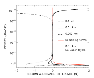
Figure 3: Percentage difference of the numerical, $N_{n}$, relative to the analytical, $N_{a}$, column abundance along a ray, as a function of the largest atmospheric density reached by that ray, for different thicknesses (0.1, 0.01, and 0.002 km - see inset legend) of MAKEXOSHELL’s computational layers. That difference is also shown for a computational layer thickness of 0.01 km when the numerical contribution from the upper layers (see equation 59) is not included (long-dashed line). The red curve shows our estimated contribution from the higher-order terms, $N_{rest}$ (see equation 45).

At lower densities, significant errors occur near the atmospheric top boundary and the numerical algorithm finds larger column abundance than the analytical solution. This is due to our imperfect way of incorporating the contribution of the upper layers. However, not including it causes much larger errors (see the long-dashed line). One solution is to adjust the top boundary to confine these errors to atmospheric regions with densities low enough that they have negligible optical depths, and make no impact on the interpretation of remote sensing observations.

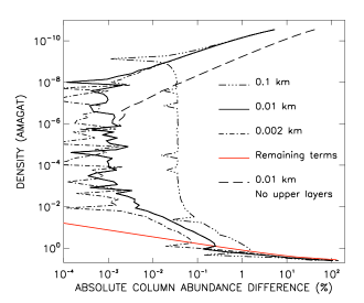
Figure 4: Absolute percentage difference of the numerical, $N_{n}$, relative to the analytical, $N_{a}$, column abundance along a ray, as a function of the largest atmospheric density reached by that ray, for different thicknesses (0.1, 0.01, and 0.002 km - see inset legend) of MAKEXOSHELL’s computational layers. See the caption in Fig. 3.

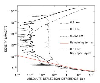
Figure 5: Absolute percentage difference of the numerical, $\omega_{n}$, relative to the analytical, $\omega_{a}$, ray deflection, as a function of the largest atmospheric density reached by that ray, for different thicknesses (0.1, 0.01, and 0.002 km - see inset legend) of MAKEXOSHELL’s computational layers. That difference is also shown for a computational layer thickness of 0.01 km when the numerical contribution from the upper layers (see equation 60) is not included (long-dashed line). The red curve shows our estimated contribution from the higher-order terms, $\omega_{rest}$ (see equation 46).

At higher densities, the absolute difference in the column abundance increases and seems to follow a density power law, until it reaches about 0.3 per cent around 1 amagat. In these density regions, the numerical results are still lower than the analytical expressions. We have investigated whether this could be due to an inadequate computational grid resolution, and have done calculations for vertical computational layer thicknesses, $\Delta z_{comp}$, of 0.1 and 0.002 km (see the triple-dot dashed and the dot-dashed lines, respectively, in Fig. 3 through 5). The computational grid resolution does indeed play a role, as the differences between numerical and analytical results decrease markedly when changing the layer thickness from 0.1 to 0.002 km. Our choice of 0.01 km is a compromise between accuracy and computational memory requirements, with 740 to 790 computational layers per atmospheric scale height.

For densities higher than about 1 amagat, the numerical results are higher than the analytical expressions because the analytical expressions are missing the higher-order terms, and the difference increases dramatically with density as the lower boundary is approached. Although generally lower, it follows the same trend as our crude order of magnitude estimate of the contribution from these higher-order terms (see equation 45), shown by the red curve.

Differences between the numerical results and the analytical expressions of the ray deflection (see Fig. 5) are generally higher than for column abundances, but follow roughly the same behaviour. The higher-order terms becomes non-negligible at densities starting around 0.15 amagat and the difference in ray deflection is about 1.6 per cent at 1 amagat.

The excellent agreement between MAKEXOSHELL and our analytical expressions, in density regions where the higher-order terms are negligible, validates both methods simultaneously. However, the analytical expressions can only be used to compute the column abundance along the ray, and its deflection with good accuracy up to densities of about 1 and 0.15 amagat, respectively. On the other hand, MAKEXOSHELL can be used in denser regions where it captures qualitatively the expected location of a singularity near the lower boundary, as well as under more general conditions such as when gravity changes with altitude and the temperature profile is not isothermal. Indeed, MAKEXOSHELL’s only assumption is that the atmospheric density scale height is constant within each layer of the input model atmosphere, which is approximately true if the vertical sampling of the model atmosphere is high enough.

Our analytical expressions are nevertheless very useful. They first provide a benchmark against which numerical models can be compared. Indeed, we converged on the current numerical algorithm and vertical computational resolution precisely because we could compare to our improved analytical expressions. They also allow derivation of analytical expressions for other quantities which depend on the column abundance or the ray deflection, as well as allow propagation of input parameter uncertainties, both of which are crucial for atmospheric retrieval algorithms.

4.2 Relevance to temperate exoplanets

4.2.1 Column abundance and ray deflection

With the validation of our analytical expression and our numerical model, we can ask to what degree does our analytical expressions and numerical model differ from the simplest analytical expressions that are used in some exoplanet atmosphere retrieval algorithm? The simplest analytical expressions are $n_{0}\sqrt{2\pi Hr_{0}}$ for the column abundance, and $\nu_{0}\sqrt{2\pi r_{0}/H}$ for the ray deflection. These are the leading term in our analytical expressions (see equations 43 and 44). We consider this question both for the Earth-like planet that we have already described, as well as for a temperate Jovian-like planet.

Our temperate Jovian-like planet combines atmospheric model C with Jupiter’s radius and bulk mass ($R_{P}~{}=~{}69911$ km; $M_{P}~{}=~{}1.8986~{}\times~{}10^{27}$ kg), and orbits a Sun-like star at Earth’s orbital distance. Since its density scale height is about five times that of our Earth-like planet, we can use a computational layer thickness of 0.05 km for MAKEXOSHELL and get similar agreements between the numerical results and our analytical expressions as for the Earth-like planet, because we have a comparable number of computational layers per scale height.

Figures 6 and 7 show the percentage difference in the column abundance and the ray deflection, respectively, computed with our models, relative to those obtained with the simplest analytical expressions. This is shown both for our analytical expressions and our numerical algorithm, and for both type of planets considered. We are not showing the difference for densities lower than $10^{-5}$ amagat because it is constant, except close to the top boundary where these quantities are overestimated by MAKEXOSHELL (such as in figures 3 through 5).

The curves for both types of planets are remarkably similar except at densities lower than $10^{-2}$ amagat. The difference in those density regions comes from the $C_{0}$ and the $D_{0}$ coefficients in equations 43 and 44, which are power series of the ratio $(H/r)$. The similarities of these curves for both planets at deeper densities is fortuitous as the factor of 2 difference in $(r/H)$ is almost compensated by differences in refractivities, so that the dimensionless parameter $(r\nu/H)$ of these two planets is roughly the same at similar densities. Consequently, the lower boundary occurs on the temperate Jupiter at a density of 4.15 amagat (or pressure of 3.87 atm), only marginally denser than on the Earth-like planet, at an altitude of $-52.32$ km.

For both planets, the simplest analytical expressions underestimate the column abundance and ray deflection by about 1 per cent around densities of 0.1 amagat ($\approx$0.1 atm), 10 per cent around 1 amagat ($\approx$1 atm), and this error increases dramatically as rays approach the lower boundary, where $(r\nu/H)$ is equal to one. Thus, in the denser atmospheric regions, the simple expressions are quite inaccurate.

4.2.2 Effective exoplanet radius

Can these regions be observed in a transiting exoplanet, or are the optical depths there so high that these differences have no impact on an exoplanet’s effective radius? When stellar limb darkening is ignored, the effective radius, $R_{eff}$, of an exoplanet occulting the centre of its host star is given by

$$R_{eff}^{2}=b_{max}^{2}-2\int_{b_{min}}^{b_{max}}e^{-\tau}bdb$$ (69)

where $\tau=\sigma N$ is the optical thickness traversed by a ray, $\sigma$ is an average atmospheric extinction cross section, and $b_{max}$ is the impact parameter of rays grazing the top of the atmosphere. $b_{min}$ is the impact parameter of rays grazing either the critical altitude or the planetary surface, whichever is larger. For a cloud-free homogeneous isothermal atmosphere, when one ignores refraction, the effective radius of an exoplanet occurs where grazing rays have traversed an optical thickness of about 0.56 (Lecavelier des Etangs et al. 2008). This result is sensitive roughly to four atmospheric scale height (Griffith, 2014), where the atmospheric transmission $e^{-\tau}$ changes from 0.05 to 0.95, and column abundances are 5.4 and 0.1 times larger than at the effective radius, respectively.

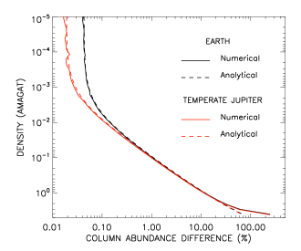
Figure 6: Percentage difference of the numerical (solid line) and analytical (dashed line) ray column abundance relative to that from the analytical expression $n_{0}\sqrt{2\pi Hr_{0}}$, as a function of the largest density reached by a ray, for Earth-like (black) and temperate Jovian-like (red, see text) planets.

As opacities change with wavelength, so does the effective radius of the exoplanet. A clear Rayleigh scattering atmosphere free of other sources of opacity produces the smallest effective radius. The average Rayleigh cross section are about $4.0\times 10^{-28}$ cm² and $7.5\times 10^{-29}$ cm² at 1 µm, for an Earth-like and Jovian-like composition, respectively. The smallest effective radius at that wavelength then occurs where the column abundance along the ray are $1.4\times 10^{27}$ cm^-2 and $7.4\times 10^{27}$ cm^-2, respectively. The largest effective radius of a cloud-free Earth in the NIR occurs in the core of a CO₂ band at $4.3~{}\micron$ at a column abundance of about $3.5\times 10^{23}$ cm^-2 (Bétrémieux & Kaltenegger, 2014), which we will use as a rough guideline of the largest value in the NIR of the effective radius of a planet for the discussion throughout this paper. If one is interested in far ultraviolet spectral features, higher altitude regions of the atmosphere are actually of importance.

It is important to stress that the various column abundances quoted above are meant only as indicators to roughly translate the size of spectral features produced by Earth’s atmosphere into equivalent features in other types of atmosphere, as well as get a feel for the range of atmospheric densities that contribute significantly to the creation of spectral features. They are in no way a substitute for actual radiative transfer calculations. In figures 8 through 15, the triple-dot-dashed lines bracket the grazing altitude corresponding to the smallest and largest effective radius using the simple column abundance criterion described above, as well as the range of ray deflection in that region. The thick blue vertical lines bracket the range of column abundances to which these spectral features are sensitive, from about 10 times lower than at the largest effective radius to about 5.4 times larger than at the smallest effective radius. If our refractive model modifies substantially the column abundance within this region, then the conditions for the validity of Lecavelier des Etangs et al. (2008)’s result breaks down and the effective radius of the exoplanet will hence be modified.

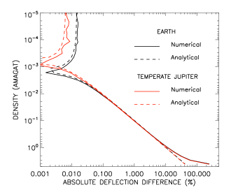
Figure 7: Absolute percentage difference of the numerical (solid line) and analytical (dashed line) ray deflection relative to that from the analytical expression $\nu_{0}\sqrt{2\pi r_{0}/H}$, as a function of the largest density reached by a ray, for Earth-like (black) and temperate Jovian-like (red, see text) planets. Note that the two minima around $10^{-3}$ amagat indicate a transition to negative differences which occur at lower densities.

Figures 8 through 11 show the ray column abundance and deflection computed with MAKEXOSHELL for our isothermal Earth-like and temperate Jovian-like atmosphere, as a function of a ray’s grazing altitude. These are shown both for atmospheric models B and D where gravity changes with altitude (solid line) and for models A and C where it is kept constant at its surface value (dashed line). Note that in all these simulations, the contribution from the upper layers are included.

For both of these temperate planets, the density scale height is much smaller than their radius, so that the variation of gravity with altitude does not make much of a change to the column abundances or ray deflection in the atmospheric regions that create spectral features. However, these regions include high density regions where our treatment of refraction computes column abundances which are at least 4 times larger than those computed with the simple analytical expressions used by Lecavelier des Etangs et al. (2008). Hence, our treatment of refraction will modify the value of a transiting temperate exoplanet’s effective radius at wavelengths where opacities are low.

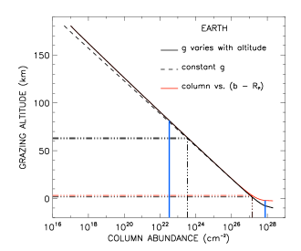
Figure 8: Ray column abundance as a function of the grazing altitude of a ray, for the Earth-like isothermal atmosphere described in sections 4.1 and 4.2, when gravity varies with altitude (solid line), and when gravity is constant (dashed line). The red line is identical to the solid line except that it is plotted as a function of the projected distance to the reference planetary radius with respect to the observer. The triple-dot-dashed lines bracket the likely effective radii of spectral features, and the vertical blue line bracket the range of column abundances to which these spectral features are sensitive (see section 4.2.2).

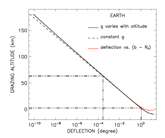
Figure 9: Ray deflection as a function of the grazing altitude of a ray, for the Earth-like isothermal atmosphere described in sections 4.1 and 4.2. See the caption in Fig. 8.

4.2.3 Effective versus actual scale height

Furthermore, the effective radius depends on the variation of the column abundance along the ray with respect to its impact parameter, and not to the grazing altitude of a ray. When plotted versus the impact parameter (or in this case versus $b-R_{P}$, which is equivalent), both the column abundance and the ray deflection display a behaviour in the denser regions which is characteristic of a much smaller scale height (as shown by the solid red curve). The effective radius of the exoplanet reaches asymptotically a value, and thus effectively mimics a surface, which is characteristic of a much smaller density than the highest density that can be probed. For our isothermal Earth atmosphere, the lower boundary, located at a density of 4.03 amagat, maps to an impact parameter 2.4 km below our 1 atm reference. If one ignores this effect, one concludes that this impact parameter correspond to a density of only about 1.38 amagat. In the temperate Jovian-like atmosphere, the lower boundary, located at a density of 4.15 amagat maps to an impact parameter 12.7 km below our 1 atm reference, or an apparent density of 1.43 amagat.

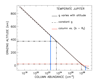
Figure 10: Ray column abundance as a function of the grazing altitude of a ray, for the temperate Jovian-like isothermal atmosphere described in section 4.2. See the caption in Fig. 8.

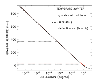
Figure 11: Ray deflection as a function of the grazing altitude of a ray, for the temperate Jovian-like isothermal atmosphere described in section 4.2. See the caption in Fig. 8.

These effects are due to the refractive deflection of the ray, and an altitude interval maps to increasingly smaller impact parameter interval for larger densities. Indeed this can be seen mathematically by differentiating equation 1 with respect to $r_{0}$, and then using equations 7 evaluated at $r_{0}$ to obtain,

$$\frac{db}{dr_{0}}=1+\nu_{0}\left(1-\frac{r_{0}}{H}\right).$$ (70)

A ray that traverses the atmosphere must satisfy equation 9, which results in $(db/dr_{0})>0$. In the upper regions of the atmosphere where refractivities tend to 0, this derivative tends to 1, and altitude intervals are almost identical to impact parameter intervals. Near the lower boundary, this ratio tends to 0, so that an altitude interval maps to a vanishingly small impact parameter interval, thus forming what amounts to a refractive boundary layer.

For our isothermal Earth atmosphere, the effective scale height of the observed column abundance has an average value of 4.3 km between 1.1 and 1.5 amagat, 1.8 km between 2.1 and 2.9 amagat, and only 0.32 km between 2.9 and 4.0 amagat, in contrast to the actual scale height of the atmosphere of about 7.4 km. A similar rapid decrease in the effective scale height occurs for the temperate Jovian atmosphere. When expressed in term of the planet’s effective radius, the size of spectral features in transmission spectroscopy scale to first order with the effective scale height. This implies that features that originate in those dense region, such as those from dimers or collision induced absorption, will appear that much smaller and will be harder to detect.

Table 3: Given and derived parameters for HD189733b

	References
Parameters	B2005	T2008	S2010
Given
R∗ (R⊙)	0.760	0.756	0.752
M∗ (M⊙)	0.820	0.806	0.840
T∗ (K)	5050	5040	5050
RP (RJ)	1.26	1.138	1.151
MP (MJ)	1.15	1.144	1.150
a (AU)	0.0313	0.0310	0.03142
Derived
$\rho$ ($\times 10^{3}$ kg m-3)	0.763	1.030	1.000
$g_{s}$ (m s-2)	18.76	22.90	22.50
Te (K), $\Lambda_{B}=0$	1200	1200	1191
Te (K), $\Lambda_{B}=0.3$	1098	1098	1090
Te (K), $\Lambda_{B}=0.5$	1009	1009	1002
Te (K), $\Lambda_{B}=0.75$	848.6	848.8	842.5
$\omega_{c}$ (°)	7.572	7.504	7.381

How much of an impact this effect has on the transit lightcurve depends on the part of the transit. When the planet occults the centre of its star, one can not observe atmospheric regions denser than the critical density of the planet (Bétrémieux & Kaltenegger, 2014). During the course of the transit, the symmetry is broken, and one part of the planet’s limb can be probed to higher densities while the opposite limb can only be probed to lower densities. If the critical density of the planet occurs at a density where the effective scale height is not significantly different from the actual scale height, then this apparent decrease of the scale height of the denser regions may not be observed, except possibly at the edges of the transit.

For a given column abundance, the Earth-like planet bends radiation more than the temperate Jovian-like planet. For instance, at a column abundance of $3.5\times 10^{23}$ cm^-2, the ray deflection are about $2.8\times 10^{-4}$ and $2.5\times 10^{-5}$ degree, respectively, roughly a factor of 11 difference. The critical density to which one can probe the atmosphere during an exoplanet transit is higher for the temperate Jovian-like planet. Around a G2 star, the critical densities are 0.22 and 0.36 amagat for the Earth-like and the temperate Jovian-like planets, respectively. Around an M9 star (R${}_{*}=0.08$ R_⊙; T${}_{*}=2300$ K), the planet must have a semi-major axis of 0.0127 AU, in order to receive the same flux as a planet 1 AU from a G2 star. Since the planetary radii are comparable to the stellar radius, the critical deflections of the two planets are markedly different (1.87°and 3.79°, respectively) and so are the critical densities (1.32 and 3.00 amagat, respectively), which are high enough that the effective scale height of the atmosphere is significantly different from the actual scale height.

As our treatment of refraction makes a difference for temperate planets, we will now investigate whether this is also the case for hotter exoplanets which are more easily observed. As an example, we will consider two planets that have already been repeatedly observed: the hot Jupiter HD189733b and the super-Earth GJ1214b.

4.3 HD189733b

The NASA Exoplanet Archive (Akeson et al., 2013) lists three references for the system parameters of HD189733b and its host stars: its discovery by Bouchy et al. (2005), and further observations and reanalysis by Torres et al. (2008), and Southworth (2010). Table 3 lists some of those parameters, as well as the mean mass density, $\rho$, surface gravity, $g_{s}$, the mean emission temperature for various Bond albedo, $T_{e}(\Lambda_{B})$, of the planet, and the critical deflection, $\omega_{c}$, of the planet-star system (see Bétrémieux & Kaltenegger 2014 for its definition), that we derive from these parameters. Note that we list the temperature for albedos between 0 and 0.75, the same range considered by Charbonneau et al. (2009) and Anglada-Escudé et al. (2013) for GJ1214b. Since its discovery, the planetary and stellar parameters of the HD189733 system have evolved quite substantially, but nevertheless the mean mass density and surface gravity of the planet from the parameters of Torres et al. (2008) and Southworth (2010) are very similar. What is very uncertain remains the temperature of the atmosphere, as this depends on the composition of minor species and whether clouds and aerosols are present. Hence, it is not worth to get into a discussion about whose planetary and stellar parameters are the best, as they do not dominate the uncertainties of the atmospheric properties, and we will merely use the revised parameters of Southworth (2010) to get a sense of what effects are of importance.

We combine the planetary parameters (radius and mass) of HD189733b listed under S2010 in Table 3, with atmosphere models E and F. Figures 12 and 13 show the ray column abundance and deflection as a function of the grazing altitude of a ray. Altitude regions where the effective scale height decreases dramatically is below the modelled regions. Just above our 10 atm “surface”, the average effective scale height between 1.82 and 2.50 amagat is 146.1 km while the actual density scale height is 174.5 km. The densities at a given pressure are about a factor of 4.3 lower than for our temperate planets because the temperature is so much higher. Consequently, $(r\nu/H)$ never reaches unity, even at the “surface” where it is only about 0.14, and column abundance and ray deflection are increased by about 6 per cent by our treatment of refraction compared to the simplest analytical expressions.

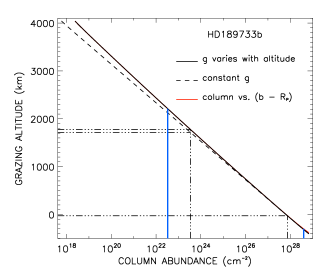
Figure 12: Ray column abundance as a function of the grazing altitude of a ray for the Jovian-like isothermal atmosphere of HD189733b described in section 4.3, using the S2010 parameters of Table 3. See the caption in Fig. 8.

The critical deflection of the planet-star system is about 7.4°(see bottom of Table 3), larger than the surface deflection of about 1.0°. Consequently, the critical altitude will occur below our “surface”, and thus below the regions to which spectral features are sensitive (see blue vertical lines in Fig. 10). Hence, refraction does not prevent any part of the atmosphere from being observed at wavelengths below 1 µm. Although Rayleigh scattering cross sections decrease with the fourth power of the wavelength, many molecular absorption lines exist in the infrared, and are usually the dominant source of opacity.

Given our simple column abundance criterion (see section 4.2.2), the larger effective radius of the non-constant gravity model is 60 km larger than the constant gravity model, or about a third of a scale height, which translates into an extra stellar flux drop of $3.5\times 10^{-3}$ per cent during transit. Since this is smaller than uncertainties in observations of HD189733b to date (see e. g. Fig. 4 in McCullough et al. 2014), this effect is not important for current exoplanet observations, but might be for future James Webb Space Telescope observations.

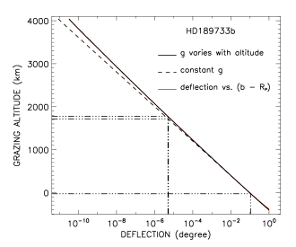
Figure 13: Ray deflection as a function of the grazing altitude of a ray for the Jovian-like isothermal atmosphere of HD189733b described in section 4.3, using the S2010 parameters of Table 3. See the caption in Fig. 8.

4.4 GJ1214b

The NASA exoplanet archives list a few references for the system parameters of GJ1214b and its host star: its discovery by Charbonneau et al. (2009), and further observations by Carter et al. (2011), Harpsøe et al. (2013), and Anglada-Escudé et al. (2013). Table 4 lists the given parameters from these different sources, as well as the mean mass density, surface gravity, average emission temperature, and critical deflection, that we derive from them (see section 4.3 for symbol definitions). Of these observations, Anglada-Escudé et al. (2013) uses recent parallax observations to re-evaluate the distance of the system, and combines it with new radial velocity measurements and transit observations to refine the system parameters. The derived planetary parameters are very similar to those previously obtained by Harpsøe et al. (2013), namely a low mean density and small surface gravity, but with higher temperatures than previously found. In this section, we will use their “maximum probability” planetary parameters (radius and mass) listed under AE2013 in Table 4 with atmospheric models G and H.

Figures 14 and 15 show the ray column abundance and deflection as a function of the grazing altitude of a ray. At the “surface”, $(r\nu/H)$ is 0.044, smaller than the value for HD189733b, and our treatment of refraction makes even less of a difference than for HD189733b. Indeed, column abundances at the “surface” are increased by about 3 per cent, and ray deflections by 1 per cent, by our treatment of refraction. The ray deflection at the surface is about 0.76°, far less than the critical deflection of 4.4°, and the critical altitude is below our “surface”. Hence, for a Jovian composition, refraction does not prevent any part of the atmosphere of GJ1214b from being observed.

Table 4: Given and derived parameters for GJ1214b

	References
	Ch2009	Ca2011	Ca2011	H2013	AE2013	AE2013
		Method A	Method B		Maximum	Expected
Parameters					probability	value
Given
R∗ (R⊙)	0.211	0.210	0.179	0.216	0.213	0.211
M∗ (M⊙)	0.157	0.157	0.156	0.150	0.176	0.176
T∗ (K)	3026	3170	3170	3026	3252	3252
RP (RE)	2.678	2.65	2.27	2.85	2.80	2.72
MP (ME)	6.55	6.45	6.43	6.26	6.26	6.19
a (AU)	0.01439	0.01437	0.01225	0.01411	0.01449	0.01435
Derived
$\rho$ ($\times 10^{3}$ kg m-3)	1.88	1.91	3.03	1.49	1.57	1.70
$g_{s}$ (m s-2)	8.97	9.02	12.25	7.57	7.84	8.22
Te (K), $\Lambda_{B}=0$	559	584	584	571	601	601
Te (K), $\Lambda_{B}=0.3$	511	535	535	522	550	550
Te (K), $\Lambda_{B}=0.5$	470	491	491	480	506	506
Te (K), $\Lambda_{B}=0.75$	395	413	413	404	425	425
$\omega_{c}$ (°)	4.367	4.349	4.351	4.578	4.394	4.386

However, the combination of a high temperature with a low gravity and a low mean molecular mass creates a scale height which is a non-negligible fraction of the planetary radius. As a result, the variation of gravity with altitude makes quite a difference to the density altitude profile and to the resulting column abundances. Indeed, in order for atmospheric model H to have comparable densities at the upper boundary as models B, D, and F, its atmospheric thickness must be significantly larger (see Table 2). Ignoring the variation of gravity with altitude causes a drop in the column abundance of 5 orders of magnitude at that upper boundary, whereas it is less than 1 order of magnitude for the other models.

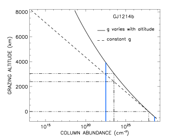
Figure 14: Ray column abundance as a function of the grazing altitude of a ray for the Jovian-like isothermal atmosphere of GJ1214b described in section 4.4, using the AE2013 maximum probability parameters of Table 4. See the caption in Fig. 8.

The size of spectral features increases by about 655 km when considering the effect of a non-constant gravity with altitude, or $0.44$ per cent of the stellar radius, which is comparable to uncertainties in recent observations (see e.g. Fig. 4 in de Mooij et al. 2013, and references therein). However, one should then also expect spectral features to change the effective radius of the planet by about 3050 km, or about 2 per cent of the stellar radius, rather than the 0.6 per cent that has been observed to date.

Figure 15: Ray deflection as a function of the grazing altitude of a ray for the Jovian-like isothermal atmosphere of GJ1214b described in section 4.4, using the AE2013 maximum probability parameters of Table 4. See the caption in Fig. 8.

We will not try here with our illustrative model to solve the mystery of GJ1214b’s atmospheric composition but we will merely point out, as done by many previous analyses (see e.g. Bean et al. 2010; Croll et al. 2011; Crossfield, Barman & Hansen (2011); Fraine et al. 2013; de Mooij et al. 2013; Kreidberg et al. 2014), that a haze or cloud layer is a possible solution. Indeed, the top of that layer would probably determine the lowest altitude that could be observed, rather than Rayleigh scattering, decreasing the altitude range available for formation of spectral features. Incidently, our zero altitude reference pressure would also be correspondingly lower, shifting the densities in our atmospheric model to smaller heights.

5 Summary and conclusions

We have derived new analytical expressions for the column abundance along a ray refracted by a planetary atmosphere with a constant density scale height, as well as the deflection experienced by that ray. These expressions were obtained by doing a Taylor power-series expansion of the exact integral formulation to the second order of the highest refractivity reached by the refracted ray. Surprisingly, the resulting analytical expression is not dependent on powers of the refractivity, but rather on powers of the dimensionless parameter $(r\nu/H)$. Although the refractivity is typically small, this dimensionless parameter is not necessarily so, and higher-order terms are dominant in a temperate atmosphere when rays reaches densities larger than about 1 and 0.15 amagat for the column abundance and the deflection, respectively. We have thus also derived an analytical expression that gives a rough estimate of the contribution from these higher-order terms.

Since the scale height of most atmospheres are usually not constant, we have also developed a new numerical algorithm, MAKEXOSHELL, to trace rays through a spherically symmetric atmosphere given the STP refractivity of the atmosphere and an arbitrary one-dimensional temperature-pressure profile. We have compared the results of numerical simulations to values obtained with our analytical expressions for a 10 atm 255 K isothermal Earth-like atmosphere on a planet with a size and mass identical to Earth’s. We have found that there is a better than 0.004 per cent agreement for densities up to $6\times 10^{-3}$ amagat, both for the computed column abundance and the ray deflection, except near our upper atmospheric boundary where densities are extremely low, and in the denser regions where the higher-order terms dominate. The excellent agreement, between our analytical expressions and numerical results, validates both methods simultaneously.

We have built a few simple isothermal atmospheric models (temperate Earth-like planet, temperate Jovian-like planet, GJ1214b, and HD189733b) to determine the type of transiting exoplanets where our treatment of refraction, as well as the variation of gravity with altitude, makes an impact on their effective radius. The effects of a non-constant gravity with altitude are more pronounced for atmospheres where the atmospheric scale height is not much smaller than the planetary radius. The combination of a hot temperature with a low gravity and mean molecular mass, creates the proper condition in a Jovian-composition GJ1214b. If GJ1214b’s atmosphere had a cloud or haze-free Jovian composition, the difference in density profile due to the variation in gravity is sufficiently large that the resulting change in effective radius at high opacities is comparable to current observational uncertainties. It is far less important for HD189733b, and negligible for both temperate planets.

The difference in the computed column abundance and the ray deflection, between our numerical treatment of refraction and simple analytical expressions used in current exoplanet atmosphere retrieval algorithms, increases with the dimensionless parameter $(r\nu/H)$, and thus with the largest atmospheric density reached by a ray. We find that for hot Jupiters, such as HD189733b, as well as a Jovian-composition GJ1214b, atmospheric regions to which spectral features are sensitive are not dense enough for our improved treatment of refraction to make much of an impact. However, for temperate isothermal atmospheres of Earth-like and Jovian-like planets, the difference is about 1 per cent at 0.1 amagat, 10 per cent at 1 amagat, and increase dramatically at larger densities, which can impact spectral features.

The column abundance and ray deflection tend toward infinite values, thus forming a refractive boundary layer, as the deepest region that can be probed by transmission spectroscopy and stellar occultation is approached. This lower boundary occurs where the radius of curvature of a grazing ray exactly matches the radial position of the ray with respect to the centre of the planet, and is only dependent on the density profile of the planet’s atmosphere. Rays that reach this boundary will spiral deeper into the atmosphere and be absorbed. The critical altitude discussed in Bétrémieux & Kaltenegger (2014), can never be lower than this lower boundary no matter how close the exoplanet is to its star.

Combined with the bending property of the atmosphere, temperate atmospheric layers with densities larger than 1 amagat have an apparent scale height significantly smaller than the actual density scale height of the atmosphere. This effective scale height tends to zero as rays approach the lower boundary. In transmission spectroscopy, spectral features scale to first order with scale height when expressed in term of the effective planetary radius. Hence, spectral features that originate in these dense regions, such as those from dimers and collision-induced absorption, will be much harder to detect. Furthermore, this interesting effect effectively mimics a surface so that even temperate giant planets seem to have a surface in spectral regions where opacities are low. This effect can only be seen for exoplanets that are close enough to their star that the critical altitude of the planet-star system approaches this lower boundary. Given that it is easier to detect a planet by transit spectroscopy around cooler stars, and that as a result many exoplanet searches now specifically target M-dwarf stars, this is more likely to be indeed the case.

References

- Akeson et al. (2013) Akeson R. L., Chen X., Ciardi D., Crane M., Good J., et al., 2013, PASP, 125, 989A
- Anglada-Escudé et al. (2013) Anglada-Escudé G., Rojas-Ayala B., Boss A. P., Weinberger A. J., Lloyd J. P., 2013, A&A, 551, A48
- Arfken (1985) Arfken G., 1985, Mathematical methods for physicists - Third edition, Academic Press, Inc., Oxford, Ohio
- Arnold et al. (2014) Arnold L., Ehrenreich D., Vidal-Madjar A., Dumusque X., Nitschelm C., Querel R. R., et al., 2014, A&A, 564, A58
- Auer & Standish (2000) Auer L. H., Standish E. M., 2000, ApJ, 119, 2472
- Bates (1984) Bates D. R., 1984, P&SS, 32, 785
- Bean et al. (2010) Bean J. L., Miller-Ricci Kempton E., Homeier D., 2010, Nature, 468, 669 2012, ApJ, 753, 100
- Benneke & Seager (2012) Benneke B., Seager S., 2012, ApJ, 753, 100
- Bétrémieux & Kaltenegger (2013) Bétrémieux Y., Kaltenegger L., 2013, ApJL, 772, L31
- Bétrémieux & Kaltenegger (2014) Bétrémieux Y., Kaltenegger L., 2014, ApJ, 791, 7
- Bouchy et al. (2005) Bouchy F., Udry S., Mayor M., Moutou C., Pont F., Iribarne N., et al., 2005, A&A, 444, L15
- Carter et al. (2011) Carter J. A., Winn J. N., Holman M. J., Fabrycky D., Berta Z. K., et al., 2011, ApJ, 730, 82
- Charbonneau et al. (2009) Charbonneau D., Berta Z. K., Irwin J., Burke C. J., Nutzman P., Buchhave L. A., et al., 2009, Nature, 462, 891
- Croll et al. (2011) Croll B., Albert L., Jayawardhana R., Miller-Ricci Kempton E., Fortney J. F., et al., 2011, ApJ, 736, 78
- Crossfield et al. (2011) Crossfield I. J. M., Barman T., Hansen B. M., 2011, ApJ, 736, 132
- de Mooij et al. (2013) de Mooij E. J. W., Brogi M., de Kok R. J., Snellen I., Croll B., et al., 2013, ApJ, 771, 109
- de Wit & Seager (2013) de Wit J., Seager S., 2013, Science, 342, 1473
- Ehrenreich et al. (2014) Ehrenreich D., Bonfils X., Lovis C., Delfosse X., Forveille T., Mayor M., Neves V., Santos N. C., Udry S., Ségransan D., 2014, A&A, preprint (arXiv:1405.1056v4)
- Ford & Browne (1973) Ford A. L., Browne J. C., 1973, Atomic data, 5, 305
- Fortney (2005) Fortney J.J., 2005, MNRAS, 364, 649
- Fraine et al. (2013) Fraine J. D., Deming D., Gillon M., Jehin E., Demory B.-O., et al., 2013, ApJ, 765, 127
- García Muñoz et al. (2012) García Muñoz A., Zapatero Osorio M. R., Barrena R., Montañés-Rodríguez P., Martín E. L., Pallé E., 2012, ApJ, 755, 103
- Goldsmith (1963) Goldsmith D. W., 1963, Icar, 2, 341
- Griffith (2014) Griffith C.A., 2014, Phil. Trans. R. Soc. A, doi: 10.1098/rsta.2013.0086
- Harpsøe et al. (2013) Harpsøe K. B. W., Hardis S., Hinse T. C., Jørgensen U. G., Mancini L., et al. 2013, A&A, 549, A10
- Howe & Burrows (2012) Howe A.R., Burrows A.S., 2012, ApJ, 756, 176
- Hui & Seager (2002) Hui L., Seager S., 2002, ApJ, 572, 540
- Kreidberg et al. (2014) Kreidberg L., Bean J. L., Désert J.-M., Benneke B., Deming D., et al. 2014, Nature, 505, 69
- Lecavelier des Etangs et al. (2008) Lecavelier des Etangs A., Pont F., Vidal-Madjar A., Sing D., 2008, A&A, 481, L83
- Lodders & Fegley, Jr. (1998) Lodders K., Fegley Jr. B., 1998, The Planetary Scientist’s Companion, New York:Oxford University Press
- Mansfield & Peck (1969) Mansfield C. R., Peck E. R., 1969, J. Opt. Soc. Am., 59, 199
- McCullough et al. (2014) McCullough P. R., Crouzet N., Demming D., Madhusudhan N., 2014, ApJ, 791, 55
- Misra, Meadows & Crisp (2014) Misra A.K., Meadows V.S., 2014, ApJL, 795, L14
- Misra & Meadows (2014) Misra A., Meadows V., Crisp D., 2014, ApJ, 792, 61
- Pallé et al. (2009) Pallé E., Zapatero Osorio M. R., Barrena R., Montañés-Rodríguez P., Martín E. L., 2009, Nature, 459, 814
- Phinney & Anderson (1968) Phinney R.A., Anderson D.L., 1968, JGR, 73, 1819
- Sidis & Sari (2010) Sidis O., Sari, R., 2010, ApJ, 720, 904
- Smith & Hunten (1990) Smith G. R., Hunten D. M., 1990, Rev. Geophys., 28, 117
- Southworth (2010) Southworth J., 2010, MNRAS, 408, 1689
- Torres et al. (2008) Torres G., Winn J. N., Holman M. J., 2008, ApJ, 677, 1324
- Vidal-Madjar et al. (2010) Vidal-Madjar A., Arnold L., Ehrenreich D., Ferlet R., Lecavelier des Etangs A., et al. 2010, A&A, 523, A57
- Waldmann et al. (2014) Waldmann I.P., Tinetti G., Barton E.J., Yurchenko S.N., Tennyson J., 2014, ApJ, preprint (arXiv:1409.2312v1)
- Weber (2003) Weber M. J., 2003, Handbook of optical materials, CRC Press LLC, Boca Raton, Florida