Iterative methods for the delay Lyapunov equation with T-Sylvester preconditioning

Abstract

The delay Lyapunov equation is an important matrix boundary-value problem which arises as an analogue of the Lyapunov equation in the study of time-delay systems $\dot{x}(t)=A_{0}x(t)+A_{1}x(t-\tau)+B_{0}u(t)$. We propose a new algorithm for the solution of the delay Lyapunov equation. Our method is based on the fact that the delay Lyapunov equation can be expressed as a linear system of equations, whose unknown is the value $U(\tau/2)\in\mathbb{R}^{n\times n}$, i.e., the delay Lyapunov matrix at time $\tau/2$. This linear matrix equation with $n^{2}$ unknowns is solved by adapting a preconditioned iterative method such as GMRES. The action of the $n^{2}\times n^{2}$ matrix associated to this linear system can be computed by solving a coupled matrix initial-value problem. A preconditioner for the iterative method is proposed based on solving a T-Sylvester equation $MX+X^{T}N=C$, for which there are methods available in the literature. We prove that the preconditioner is effective under certain assumptions. The efficiency of the approach is illustrated by applying it to a time-delay system stemming from the discretization of a partial differential equation with delay. Approximate solutions to this problem can be obtained for problems of size up to $n\approx 1000$, i.e., a linear system with $n^{2}\approx 10^{6}$ unknowns, a dimension which is outside of the capabilities of the other existing methods for the delay Lyapunov equation.

1 Introduction

Consider the linear single-delay time-delay system defined by the equations

(1a) $$\dot{x}(t) = A_{0}x(t)+A_{1}x(t-\tau)+B_{0}u(t)$$

(1b) $$y(t) = C_{0}x(t),$$

where $A_{0},A_{1}\in\mathbb{R}^{n\times n}$, $B_{0}\in\mathbb{R}^{n\times m}$, $C_{0}^{\mathrm{T}}\in\mathbb{R}^{n\times p}$. The general equation (1) appears in many different fields. It is considered a very important topic in the field of systems and control, mostly due to the fact that most feedback systems are non-instantaneous in the sense that there is a delay between the observation (of for instance the state) and the action of the feedback. See monographs [18, 5] and survey paper [24] for literature on time-delay systems.

The delay Lyapunov equations associated with (1) correspond to the problem of finding $U\in\mathcal{C}^{0}([-\tau,\tau],\mathbb{C}^{n\times n})$ such that

(2a) $$U^{\prime}(t) = U(t)A_{0}+U(t-\tau)A_{1},\;t>0,$$

(2b) $$U(-t) = U(t)^{\mathrm{T}},$$

(2c) $$-W = U(0)A_{0}+A_{0}^{\mathrm{T}}U(0)+U(\tau)^{\mathrm{T}}A_{1}+A_{1}^{\mathrm{T}}U(\tau),$$

hold for a given a cost matrix $W=W^{T}\in\mathbb{R}^{n\times n}$ (in some applications, for instance, $W=C_{0}^{T}C_{0}$).

Equation (2a) is a matrix delay-differential equation and (2c) is an algebraic condition involving $U(0)$, $U(\tau)$ and $U(-\tau)=U(\tau)^{T}$ such that (2) can be interpreted as a matrix boundary value problem. In this paper we propose a new procedure to solve (2), with the goal to have good performance for large $n$ ($n\approx 500-1000$, for instance).

The delay Lyapunov equation generalizes the standard Lyapunov equation, since, e.g., if we set $\tau=0$ the equation reduces to the standard Lyapunov equation. Moreover, as established by the last decades of research, the delay Lyapunov equation is in many ways playing the same important role for time-delay systems as the standard Lyapunov equation plays for standard (delay free) linear time-invariant dynamical systems. More precisely, the delay Lyapunov equation has been studied in the following ways. It has been extensively used to characterize stability of delay differential equations, as one can explicitly construct a Lyapunov functional from $U(t)$, where the solution is sometimes referred to as delay Lyapunov matrices. Sufficient conditions for stability are given in [13, 21, 20] and for neutral systems in [22], and conditions for instability in [19, 4]. It has been used to provide bounds on the transient phase of delay-differential equations in the PhD thesis [23] and [14, 15]. Existence and uniqueness of the solutions are well characterized, e.g., in [13]. See also the monograph [5]. Recently, it has been shown that in complete analogy to the standard Lyapunov equation the solution to the delay Lyapunov equation explicitly gives the $\mathcal{H}_{2}$-norm [12]. The delay Lyapunov equation can also be used to carry out a model order reduction which generalizes balanced truncation [11].

This paper concerns computational aspects of the delay Lyapunov equation. Some computational aspects are treated in the literature, e.g., the matrix exponential formula in [23], the polynomial approximation approach in [9], spectral (Chebyshev-based) discretization approaches in [12, 31] and an ODE-approach in the PhD thesis [17, Chapter 3].

In complete contrast to the delay Lyapunov equation, the computational aspects of the standard Lyapunov equation have received considerable attention, mostly in the numerical linear algebra community. Most importantly, the Bartels-Stewart method [1], ADI methods [2], Krylov methods [28, 8], and rational Krylov methods [10], including preconditioning techniques [6], have turned to be effective in various situations. For a more thorough review, see the survey [29]. To our knowledge, there exist no natural generalization of the Bartels-Stewart algorithm and there are no Krylov methods for delay Lyapunov equation.

The method we propose is tailored to medium-scale equations; it combines the use of a Krylov-type method and a direct algorithm similar to the Bartels-Stewart one. More precisely, our approach is based on a characterization of the solution to the delay Lyapunov equation as a linear system of equations with $n^{2}$ unknowns. This characterization is derived in Section 2. Since the linear system derived in Section 2 is large and only given implicitly as a matrix vector product, we propose to adapt iterative methods which are based on matrix vector products only, e.g., GMRES [27] or BiCGStab [33], to this problem. It turns out to be natural to use a preconditioner involving a matrix equation called the T-Sylvester equation, for which there are efficient $O(n^{3})$ methods for the dense case [3]. We quantify the quality of the preconditioner by deriving a bound on the convergence factor of the iterative method. The iterative method and the preconditioner are given in Section 3. The performance of the approach is illustrated with simulations in Section 4. We apply the method to a problem stemming from the discretization of a two-dimensional partial delay-differential equation (PDDE). The number of iterations appears to be essentially independent of the grid, which suggests that the preconditioner is a sensible choice for this PDDE.

We use notation which is standard for analysis of matrix equations. The vectorization operation is denoted $\operatorname{vec}(B)$, i.e., if $B=\begin{bmatrix}b_{1}&\ldots&b_{m}\end{bmatrix}\in\mathbb{R}^{n\times m}$, $\operatorname{vec}(B)^{T}=\begin{bmatrix}b_{1}^{T}&\ldots&b_{m}^{T}\end{bmatrix}$. The Kronecker product is denoted $\otimes$. Unless otherwise stated, $\|\cdot\|$ denotes the Euclidean norm for vectors and the spectral norm for matrices. We denote the Frobenius norm by $\|\cdot\|_{F}$.

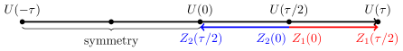
Figure 1: Graphical representation of the relation between $U(t)$, $Z_{1}(t)$ and $Z_{2}(t)$.

2 Reformulation of the delay Lyapunov equations

Our method is based on a reformulation of the delay Lyapunov equation where we define for each $t\in[0,\tau/2]$

(3) $$Z_{1}(t) :=U(\tau/2+t), Z_{2}(t) :=U(\tau/2-t).$$

The two matrix-valued functions $Z_{1}(t)$ and $Z_{2}(t)$ coincide with $U(t)$ up to a change of the time coordinate which is represented visually in Figure 1. Essentially, they represent two different branches of $U(t)$ “taking off” from $\tau/2$ in opposite directions. Note that the left half of the function, $U([-\tau,0])$, is determined uniquely by the right half $U([0,\tau])$ by the transposition symmetry condition (2b). The only nontrivial condition implied by (2b) is that $U(0)$ must be symmetric.

Note that

(4a) $$Z_{1}(t-\tau) = U(t-\tau+\tau/2)=U(t-\tau/2)=U(\tau/2-t)^{T}=Z_{2}(t)^{T}$$

(4b) $$Z_{2}(t-\tau) = U(\tau/2-t-\tau)=U(-t-\tau/2)=U(t+\tau/2)^{T}=Z_{1}^{T}(t)$$

Hence, the delay differential equation (2a) becomes an ordinary differential equation

(5a) $$Z_{1}^{\prime}(t) = \phantom{-}Z_{1}(t)A_{0}+Z_{2}(t)^{T}A_{1},$$

(5b) $$Z_{2}^{\prime}(t) = -Z_{1}(t)^{T}A_{1}-Z_{2}(t)A_{0}.$$

This is a constant-coefficient homogeneous linear system of ODEs which can be solved explicitly if the common (unknown) initial value $Z_{1}(0)=Z_{2}(0)=U(\tau/2)$ is provided. Using vectorization, we can give an explicit formula

(6) $$\begin{bmatrix}\operatorname{vec}Z_{1}(t)\phantom{{}^{T}}\\ \operatorname{vec}Z_{2}(t)^{T}\\ \end{bmatrix}=\exp(t\mathcal{A})\begin{bmatrix}\operatorname{vec}U(\tau/2)\phantom{{}^{T}}\\ \operatorname{vec}U(\tau/2)^{T}\end{bmatrix},$$

where

(7) $$\mathcal{A}:=\begin{bmatrix}A_{0}^{T}\otimes I_{n}&A_{1}^{T}\otimes I_{n}\\ -I_{n}\otimes A_{1}^{T}&-I_{n}\otimes A_{0}^{T}\end{bmatrix}.$$

In terms of $Z_{1}(t)$ and $Z_{2}(t)$, the algebraic condition (2c) and the symmetry condition (2b) for $t=0$ reduce to

(8a) $$0 = W+Z_{2}(\tau/2)^{T}A_{0}+A_{0}^{T}Z_{2}(\tau/2)+Z_{1}(\tau/2)^{T}A_{1}+A_{1}^{T}Z_{1}(\tau/2),$$

(8b) $$0 = Z_{2}(\tau/2)-Z_{2}(\tau/2)^{T}.$$

Notice that the right-hand side of (8a) is symmetric and that of (8b) is antisymmetric. A linear combination of them gives

(9) $$0=W+Z_{2}(\tau/2)^{T}(A_{0}-cI)+(A_{0}^{T}+cI)Z_{2}(\tau/2)+Z_{1}(\tau/2)^{T}A_{1}+A_{1}^{T}Z_{1}(\tau/2)$$

for each $c\in\mathbb{R}$, which forms the basis of our matrix operator.

Definition 1.

Let $L_{c}:\mathbb{R}^{n\times n}\rightarrow\mathbb{R}^{n\times n}$ be defined by

(10) $$L_{c}(X):=\\ Z_{2}(\tau/2)^{T}(A_{0}-cI)+(A_{0}^{T}+cI)Z_{2}(\tau/2)+Z_{1}(\tau/2)^{T}A_{1}+A_{1}^{T}Z_{1}(\tau/2)$$

where $Z_{i}:[0,\tau/2]\rightarrow\mathbb{R}^{n\times n}$, $i=1,2$ are the unique solutions to the initial value problem (5) with $Z_{1}(0)=Z_{2}(0)=X$.

We shall need the following easy linear algebra result.

Lemma 2.

Let $M=M^{T}\in\mathbb{R}^{n\times n}$ and $N=-N^{T}\in\mathbb{R}^{n\times n}$ be two matrices, one symmetric and one antisymmetric. Then, $M+N=0$ if and only if $M=N=0$.

Proof.

The ‘if’ part is trivial; let us prove the ‘only if’. Suppose $M+N=0$; then, transposing, we have also $0=M^{T}+N^{T}=M-N$. Summing and subtracting the two relations we have $2M=2N=0$. ∎

A time-delay system is called exponentially stable if $\lVert x(t)\rVert\leq\alpha\exp(-\beta t)$ for some constants $\alpha>0,\beta>0$. If this condition holds, then the solution $U(t)$ to (2) is unique [15, Theorem 4]. In this case, we can formulate the equivalence between the delay Lyapunov equation and a linear system with operator $L_{c}$.

Theorem 3 (Equivalence).

Suppose $A_{0}$ and $A_{1}$ and $\tau$ are such that (1) is exponentially stable and let $W\in\mathbb{R}^{n\times n}$ be any symmetric matrix. Let $U$ be the solution to the delay Lyapunov equations (2) and let $L_{c}$ be defined by (10). Then, for any $c\neq 0$, $X=U(\tau/2)$ is the unique solution of the linear system

(11) $$L_{c}(X)=-W.$$

Proof.

Equation (9) already shows that if $X=U(\tau/2)$ then $L_{c}(X)=-W$. It remains to prove the reverse implication. Suppose that $X$ satisfies $L_{c}(X)+W=0$; then, by Lemma 2 applied to

$$M =Z_{2}(\tau/2)^{T}A_{0}+A_{0}^{T}Z_{2}(\tau/2)+Z_{1}(\tau/2)^{T}A_{1}+A_{1}^{T}Z_{1}(\tau/2)-W,$$

$$N =c(Z_{2}(\tau/2)-Z_{2}(\tau/2)^{T}),$$

the conditions (8) hold. Define

$$\hat{U}(t)=\begin{cases}Z_{2}(\tau/2-t)&0\leq t<\tau/2,\\ Z_{1}(t-\tau/2)&\tau/2\leq t\leq\tau,\\ U(-t)^{T}&-\tau\leq t<0.\end{cases}$$

The function $\hat{U}(t)$ is continuous in $0$ by (8b), and in $\pm\tau/2$ by the choice of initial conditions, hence it is globally continuous on $[-\tau,\tau]$. Moreover, the differential equation (2a) holds for all $t\neq 0,\tau/2$. By continuity, it must also hold for these values. Hence $\hat{U}(t)$ solves (2). As we assume exponential stability, the solution is unique and hence $\hat{U}(t)=U(t)$. ∎

Since the linear system $L_{c}(X)=-W$ has a unique solution for each symmetric $W\in\mathbb{R}^{n\times n}$, we have the following result.

Corollary 4.

Suppose (1) is exponentially stable. Then, the linear operator $L_{c}$ is nonsingular for each $c\neq 0$.

A delay-free formulation of the delay Lyapunov equations has also been derived in [13, Equation (13)]. That formulation cannot be described with a linear operator in a way that can be adapted to an iterative method in the same way that we show in the following section.

3 Algorithm

We now know from the previous section that the matrix equation (11) is equivalent to the delay Lyapunov equation. By vectorizing (11), we obtain the linear system on standard form

(12) $$\operatorname{vec}L_{c}(\mathop{\operatorname{vec}^{-1}}x)=-\operatorname{vec}W,$$

where the inverse function $\mathop{\operatorname{vec}^{-1}}(x)$ maps $\operatorname{vec}X\in\mathbb{R}^{n^{2}}$ to $X\in\mathbb{R}^{n\times n}$. Let $A\in\mathbb{R}^{n^{2}\times n^{2}}$ the matrix associated to it. We know that $A$ is nonsingular by Corollary 4.

Our approach is based on specializing an iterative method for linear systems to (12). In order to specialize an iterative method for large-scale linear systems, we need two ingredients. We need an efficient procedure to compute the action corresponding to the left-hand side of (12); and we need a preconditioner. These two ingredients are described in the following two subsections.

3.1 Action of $L_{c}$

The action of the operator $L_{c}$ is defined by (5) and (10). As a consequence, the recipe to compute $L_{c}(X)$ for a given matrix $X$ is simple:

1. Compute the solutions $Z_{1}(\tau/2)$, $Z_{2}(\tau/2)$ of the linear, constant-coefficient initial-value problem (5) with initial values $Z_{1}(0)=Z_{2}(0)=X$.

2. Compute $L_{c}(X)$ using the expression (10).

In practice, a detail is crucial in the choice of the numerical algorithm for the first step. We distinguish two possible scenarios:

• We use a method with a fixed step-size and no adaptivity: for instance, the (explicit or implicit) Euler method, or a non-adaptive Runge-Kutta method. In this case, we are effectively substituting $L_{c}$ with a different operator $\hat{L}_{c}$, which replaces the differential operator in Step 1 with a finite discretization. This operator (for most classical methods) is still linear, so the theory of Krylov subspace methods can be applied without changes: we are applying a Krylov method to get an approximate solution of a nearby linear problem $\hat{L}_{c}$.

• We use an adaptive method, which can change step size along the algorithm, possibly in different ways for different initial values $X$. For instance, the Dormand-Prince method (Matlab’s ode45). While apparently the two cases are similar, the addition of adaptivity has an important consequence: the computed operator $\hat{L}_{c}$, this time, is no longer a linear operator, because in general $\hat{L}_{c}(X_{1}+X_{2})\neq\hat{L}_{c}(X_{1})+\hat{L}_{c}(X_{2})$. Indeed, for different values of the input $X$ the initial-value problems could be solved using different grids, and hence different discrete approximations of the propagation operator. The correct framework to analyze the method in this case is the one of inexact Krylov methods [30]. We present an error analysis under this framework in Section 3.3.

3.2 Preconditioning

In order to make iterative methods effective, it is common to carry out a transformation which preconditions the problem. This can often be interpreted as transforming the problem with an approximation of the inverse of the matrix/operator. We focus on a particular preconditioner obtained by solving the problem exactly when $A_{1}$ is replaced with the zero matrix. Then (10) becomes

(13) $$\tilde{L}_{c}(X):=Z_{2}(\tau/2)^{T}(A_{0}-cI)+(A_{0}^{T}+cI)Z_{2}(\tau/2),$$

and (5b) decouples from $Z_{1}$ such that

(14) $$Z_{2}^{\prime}=-Z_{2}(t)A_{0},$$

which we can solve explicitly to get $Z_{2}(\tau/2)=X\exp(-\tau A_{0}/2)$.

Let $T$ be the operator

$$T(Y)=(A_{0}^{T}+cI)Y+Y^{T}(A_{0}-cI).$$

The operator $L_{c}$ is invertible if and only $T^{-1}$ exists, and in this case we have

(15) $$\tilde{L}^{-1}_{c}(Z)=T^{-1}(Z)\exp(\tau A_{0}/2).$$

Inverting the operator $T$ correspond to solving the so-called (real) T-Sylvester equation $MY+Y^{T}N=C$. The paper [3] discusses the solvability of this equation and presents a direct $O(n^{3})$ Bartels–Stewart-like algorithm for its solution. In particular, the following result holds.

Theorem 5 ([16, Lemma 8],[3]).

Let $M,N,C\in\mathbb{R}^{n\times n}$. The equation $MX+X^{T}N=C$ has a unique solution $X$ for each right-hand side $C$ if and only if $\mu_{i}\bar{\mu}_{j}\neq 1$ for each pair $\mu_{i},\mu_{j}$ of eigenvalues of the pencil $M-\lambda N^{T}$.

In our case, $M=A_{0}^{T}+cI$, $N=A_{0}-cI$, so after a quick computation the solvability condition reduces to the following condition, which is independent of $c$.

Definition 6 (Hamiltonian eigenpairing).

We say that the matrix $A_{0}\in\mathbb{R}^{n\times n}$ has no Hamiltonian eigenpairing, if for each pair of eigenvalues $\lambda_{i},\lambda_{j}$ of the matrix $A_{0}$, we have

$$\lambda_{i}+\bar{\lambda}_{j}\neq 0.$$

A matrix has no Hamiltonian eigenpairing, for instance, if $\Re\lambda<0$ for each eigenvalue $\lambda$ of $A_{0}$, i.e., if the delay-free system obtained by setting $A_{1}=0$ is stable.

In order to characterize the convergence and quality of the preconditioner we use a fundamental min-max bound. Suppose we carry out GMRES on the matrix $A\in\mathbb{R}^{N\times N}$ with eigenvalues $\lambda_{1},\ldots,\lambda_{N}$. From [27, Proposition 4] we have the bound of the residual

$$\|r_{m+1}\|\leq\kappa(V)\varepsilon^{(m)}\|r_{0}\|,$$

where $V$ is the eigenvector matrix of $A$ (which is assumed to be diagonalizable), and

$$\varepsilon^{(m)}=\min_{p\in P_{m}}\max_{i}|p(\lambda_{i})|$$

where $P_{m}=\{p:\textrm{polynomial of degree }m\textrm{ such that }p(0)=1\}$. We now apply the standard Zarantonello bound [26, Lemma 6.26], where we assume that the eigenvalues are contained in a disk of radius $r$ centered at $c=1$, corresponding to selecting $p(z)=\frac{(c-z)^{m}}{c^{m}}$ such that $\varepsilon^{(m)}\leq r^{m}/c^{m}=r^{m}\leq\|A-I\|^{m}$. Preconditioned GMRES with preconditioner $\tilde{A}^{-1}$ is equivalent to GMRES in exact arithmetic applied to the matrix $\tilde{A}^{-1}A$ (apart from termination criteria and initialization). Therefore, a bound on $\|\tilde{A}^{-1}A-I\|$ provides a characterization of the convergence factor of preconditioned GMRES. Because of the vectorization included in our setting, bounding $\|\tilde{A}^{-1}A-I\|$ corresponds to giving an estimate for the quantity

$$\frac{\|\tilde{L}_{c}^{-1}(L_{c}(X))-X\|_{F}}{\lVert X\rVert_{F}}.$$

Our preconditioner is constructed by setting $A_{1}=0$. Therefore, we expect that the preconditioner works well if $\|A_{1}\|$ is small. This reasoning is formalized in the following result.

Theorem 7 (Quality of preconditioner).

Suppose the system (1) is exponentially stable and suppose that $A_{0}$ has no Hamiltonian eigenpairing. Let $L_{c}$ and $\tilde{L}_{c}$ be defined by (10) and (13) respectively. Then,

(16) $$\frac{\|\tilde{L}_{c}^{-1}(L_{c}(X))-X\|_{F}}{\lVert X\rVert_{F}}=\mathcal{O}(\|A_{1}\|_{2}),$$

where the constant hidden in the $\mathcal{O}(\cdot)$ notation depends only on $\lVert A_{0}\rVert$, $\tau$ and $c$.

Proof.

We invoke Lemma 10 (provided in A) to bound the left-hand side of (16)

(17) $$\frac{\left\lVert\tilde{L}_{c}^{-1}\left(L_{c}(X)\right)-X\right\rVert_{F}}{\lVert X\rVert_{F}}=\frac{\left\lVert\tilde{L}_{c}^{-1}\left(L_{c}(X)-\tilde{L}_{c}(X)\right)\right\rVert_{F}}{\lVert X\rVert_{F}}\leq\\ K\exp(\tau\|A_{0}\|/2)\frac{\left\lVert L_{c}(X)-\tilde{L}_{c}(X)\right\rVert_{F}}{\lVert X\rVert_{F}}.$$

In order to bound $L_{c}(X)-\tilde{L}_{c}(X)$ we let $Z_{1}$ and $Z_{2}$ correspond to $L_{c}(X)$, i.e., they satisfy the equations (5) with initial value $Z_{1}(0)=Z_{2}(0)=X$. We use tilde for the differential equation corresponding to $\tilde{L}_{c}(X)$, i.e., $\tilde{Z}_{2}(t)$ satisfies (14). Moreover, let $\Delta_{2}:=Z_{2}-\tilde{Z}_{2}$. We have

(18) $$\tilde{L}_{c}(X)-L_{c}(X)=\\ \Delta_{2}(\tau/2)^{T}(A_{0}-cI)+(A_{0}^{T}+cI)\Delta_{2}(\tau/2)+Z_{1}(\tau/2)^{T}A_{1}+A_{1}^{T}Z_{1}(\tau/2),$$

for which $\Delta_{2}(\tau/2)$ and $Z_{1}(\tau/2)$ can be bounded as follows. Lemma 9 provided in A tells us that

(19) $$\|Z_{1}(\tau/2)\|_{F}\leq 2\exp(\tau(\|A_{0}\|_{2}+\|A_{1}\|_{2}))\|X\|_{F}.$$

By definition, $\Delta_{2}$ satisfies the ODE

(20) $$\Delta_{2}^{\prime}(t)=-\Delta_{2}(t)A_{0}+g(t),\quad\Delta_{2}(0)=0,$$

where $g(t):=-Z_{1}(t)^{T}A_{1}.$ The variation-of-constants formula applied to (20) results in the explicit expression

$$\Delta_{2}(t)=-\int_{0}^{t}Z_{1}(s)^{T}A_{1}\exp((s-t)A_{0})\,ds.$$

Hence,

(21a) $$\|\Delta_{2}(\tau/2)\|_{F} \leq\int_{0}^{\tau/2}\lVert Z_{1}(s)^{T}A_{1}\exp((s-\tau/2)A_{0})\rVert_{F}\,ds$$

(21b) $$\leq\int_{0}^{\tau/2}\lVert Z_{1}(s)\rVert_{F}\lVert A_{1}\rVert_{2}\lVert\exp((s-\tau/2)A_{0})\rVert_{2}\,ds$$

(21c) $$\leq\tau\exp(\tau(\|A_{0}\|_{2}+\|A_{1}\|_{2}))\lVert A_{1}\rVert_{2}\exp(\tau\lVert A_{0}\rVert_{2}/2)\|X\|_{F}.$$

We now evaluate the Frobenius norm of (18) and apply the triangle inequality and the bounds (19) and (21), which shows that

(22) $$\frac{\|\tilde{L}_{c}(X)-L_{c}(X)\|_{F}}{\lVert X\rVert_{F}}=\mathcal{O}(\|A_{1}\|_{2}).$$

The hidden constant in (22) depends only on $\lVert A_{0}\rVert_{2}$, $c$, and $\tau$. The conclusion (16) follows by combining (17) and (22). ∎

3.3 Inexact Krylov theory

As described in Section 3.1, if one uses an adaptive method for the integration, then assessing convergence requires the theory of inexact Krylov methods. The inexact GMRES method for an operator $A$ is defined as the classical GMRES iteration, but with the difference that at each step $i=1,2,\dots,k$ we do not compute the action of $w_{i}=Av_{i}$ of $A$ on a vector $v_{i}$, but rather we replace it with an approximation $w^{\mathrm{inex}}_{i}=(A+E_{i})v_{i}$, for an unknown matrix $E_{i}$. The matrix $E_{i}$ can vary at each iteration. In equivalent terms, we can say that the product $Av_{i}$ is computed up to a specified accuracy $\lVert E_{i}\rVert$, since

$$\frac{\lVert w^{\mathrm{inex}}_{i}-Av_{i}\rVert}{\lVert v_{i}\rVert}=\frac{\lVert E_{i}v_{i}\rVert}{\lVert v_{i}\rVert}\leq\lVert E_{i}\rVert.$$

This process produces a Hessenberg matrix $H^{\mathrm{inex}}_{i}$, a sequence of approximations $x^{\mathrm{inex}}_{i}$ to the solution of the linear system, and a sequence of ‘fake’ residuals $r^{\mathrm{inex}}_{i}$; these fake residual values are the ones computed during the iterative method, and they do not equal in general $b-Ax^{\mathrm{inex}}_{i}$. However, the following result holds.

Theorem 8 ([30, Theorem 5.3]).

Assume that $k\leq m$ iterations of the inexact GMRES method on an operator $A\in\mathbb{C}^{m\times m}$ have been carried out, and that for some $\delta>0$ we have

$$\lVert E_{i}\rVert\leq\frac{\sigma_{\min}(H^{\mathrm{inex}}_{k})}{k}\frac{1}{\lVert r^{\mathrm{inex}}_{i-1}\rVert}\delta,\quad i=1,2,\dots,k.$$

Then, $\lVert b-Ax_{k}^{\mathrm{inex}}-r^{\mathrm{inex}}_{k}\rVert\leq\delta$.

We would like to use this result to apply an ODE solver to compute an approximation $\hat{L}_{c}$ to the operator $L_{c}$, and tuning its accuracy at each step. However, this result is somehow ineffective for a truly adaptive computation: given a target error $\delta$, the accuracy at which we need to perform the matrix-vector product at step $i$ in order to obtain it is not available until the final step. Instead, we proceed as follows. Given a target accuracy goal $\varepsilon$, we apply several steps of the inexact GMRES method, and at each step $i=1,2,\dots$ we tune its accuracy so that

$$\lVert E\rVert_{i}\leq\frac{C\varepsilon}{\lVert r^{\mathrm{inex}}_{i-1}\rVert},$$

for a given constant $C$, and we stop the method at the first step $k$ for which $\lVert r^{\mathrm{inex}}_{i-1}\rVert\leq\varepsilon$. Applying Theorem 8 with $\delta=\frac{k}{\sigma_{\min}(H^{\mathrm{inex}}_{k})}C\varepsilon$ and the triangle inequality we obtain

$$\lVert b-Ax_{k}^{\mathrm{inex}}\rVert\leq\lVert r^{\mathrm{inex}}_{k}\rVert+\frac{k}{\sigma_{\min}(H^{\mathrm{inex}}_{k})}C\varepsilon.$$

The problem of computing the preconditioned operator $\tilde{L}_{c}^{-1}L_{c}$ up to a given accuracy is in itself nontrivial. Algorithms for adaptive integration of initial-value problems such as Matlab’s ode45 can produce $(\tilde{Z}_{1}(\tau/2),\tilde{Z}_{2}(\tau/2))$ such that

$$\left\lVert\begin{bmatrix}Z_{1}(\tau/2)-\tilde{Z}_{1}(\tau/2)\\ Z_{2}(\tau/2)-\tilde{Z}_{2}(\tau/2)\end{bmatrix}\right\rVert_{F}\leq\varepsilon\left\lVert\begin{bmatrix}Z_{1}(\tau/2)\\ Z_{2}(\tau/2)\end{bmatrix}\right\rVert_{F}$$

for a given threshold $\varepsilon$; however, even before taking into account the preconditioner, computing

$$\tilde{Z}_{2}(\tau/2)^{T}(A_{0}-cI)+(A_{0}^{T}+cI)\tilde{Z}_{2}(\tau/2)+\tilde{Z}_{1}(\tau/2)^{T}A_{1}+A_{1}^{T}\tilde{Z}_{1}(\tau/2)$$

may amplify this error by a coefficient which is difficult to bound a priori. Hence we can only obtain a very weak result: if integrating the ODE (5) with relative accuracy $\frac{\varepsilon}{\lVert r^{\mathrm{inex}}_{i-1}\rVert}$ produces a relative error in $\tilde{L}_{c}(L_{c}(X))$ which is bounded by $\frac{C\varepsilon}{\lVert r^{\mathrm{inex}}_{i-1}\rVert}$ for some constant $C$, then the residual of the computed solution satisfies

$$\lVert L_{c}(X)+W\rVert_{F}\leq\lVert r^{\mathrm{inex}}_{k}\rVert+\frac{k}{\sigma_{\min}(H^{\mathrm{inex}}_{k})}C\varepsilon.$$

3.4 A residual measure

It is useful to have a method to assess the accuracy of a computed solution to the system (2). This is a nontrivial task: first of all, this is a system of delay differential equations, so trying to evaluate it on a computer requires careful approximation; moreover, even ignoring this fact, due to the nontrivial coupling conditions between the values of the function in the two parts of the interval $[0,\tau]$, it is not immediate to choose a $n\times n$ initial value, integrate the equations, and produce an associated $W$ which we can use to test the methods on a problem for which we know the exact solution.

To this purpose, we suggest a residual measure as follows. Given approximations $\tilde{U}_{0}\approx U(0),\tilde{U}_{\tau}\approx U(\tau)$ computed by a numerical method, we check that:

• integrating numerically with ode45 the ODE (5) from the initial value $t=\tau/2$ $Z_{1}(\tau/2)=\tilde{U}_{\tau},Z_{2}(\tau/2)=\tilde{U}_{0}$ to $t=0$ produces values $Z_{1}(0),Z_{2}(0)$ such that $r_{1}:=\lVert Z_{1}(0)-Z_{2}(0)\rVert_{F}$ is small (compared to $s_{1}:=\lVert Z_{1}(0)\rVert_{F}$);

• $\tilde{U}_{0}$ is such that $r_{2}:=\lVert\tilde{U}_{0}-\tilde{U}_{0}^{\mathrm{T}}\rVert_{F}$ is small (compared to $s_{2}:=\lVert\tilde{U}_{0}\rVert_{F}$); and

• the quantity $r_{3}:=\lVert\tilde{U}_{0}A_{0}+A_{0}^{\mathrm{T}}\tilde{U}_{0}+\tilde{U}_{\tau}^{\mathrm{T}}A_{1}+A_{1}^{\mathrm{T}}\tilde{U}_{\tau}+W\rVert_{F}$ is small (compared to $s_{3}:=\lVert W\rVert_{F}$).

We use the Frobenius norm here since we care about speed of computation when $n$ may reach the order of thousands. To avoid issues in cases where one of the $s_{i}$ is very small and hence its relative residual may be large, we define a global residual measure as

$$\operatorname{res}(\tilde{U}_{0},\tilde{U}_{\tau}):=\frac{r_{1}+r_{2}+r_{3}}{s_{1}+s_{2}+s_{3}}.$$

This residual measure is built on approximations to $U(0)$ and $U(\tau)$ as its inputs. It is indeed possible to construct an analogous measure starting from an approximation to $U(\tau/2)$ instead, which may look more natural in view of the development in the previous sections. However, a reader looking with critical eye may wonder if the good results obtained by the methods introduced here are due to the choice of a residual function that favors the midpoint $U(\tau/2)$ over the endpoints $U(0)$ and $U(\tau)$, since our method builds heavily on $U(\tau/2)$, while it is not a quantity that appears naturally in the competing algorithms. Thus we choose to work with $\tilde{U}_{0},\tilde{U}_{\tau}$ to get a fairer assessment of the merits of this method.

4 Simulations

4.1 A small example

In order to illustrate the preconditioner and properties of our approach we first consider a small example with randomly generated $A_{0}$ matrix. We specify the matrices for reproducibility

$$A_{0}=\begin{bmatrix}-26&22&-1&-4\\ 2&-24&-4&1\\ 7&11&-24&-22\\ -13&15&-1&-9\end{bmatrix},\;\;A_{1}=\alpha\operatorname{diag}(-1,-0.5,0,0.5),\;\;W=I$$

and $\tau=1$. We carry out simulations for different $\alpha=\|A_{1}\|$. The time-delay system is stable for all $\alpha\in[0,10]$. The corresponding delay Lyapunov equation satisfies

$$U(\tau/2)\approx\frac{1}{100}\cdot\begin{bmatrix}0.2302&-0.0156&0.0101&-0.3729\\ -0.0885&0.0044&-0.0038&0.1380\\ 0.1466&-0.0057&0.0056&-0.2263\\ -0.5485&0.0331&-0.0238&0.8755\end{bmatrix}$$

for $\alpha=1$.

We combine our approach with two different generic iterative methods for linear systems of equations, GMRES [27] and BiCGStab [33] and select $c=1$. To illustrate the properties of the performance of the iterative method, we solve the ODE defining $L_{c}$ to full precision with the matrix exponential. The absolute error as a function of iteration is given in Figure 2. Both methods successfully solve the problem before the break-down at iteration $n^{2}$ except for $\|A_{1}\|=10$. No substantial difference between the two iterative methods can be observed in the error as a function of iteration, i.e., nothing can be concluded regarding which of the two variants is better for this problem. The convergence of the two methods is faster for small $\|A_{1}\|$. This is due to the fact that the preconditioner is more effective when $\|A_{1}\|$ is small, which is consistent with Theorem 7 and Figure 3, where we clearly see that the norm of the preconditioned system $X\mapsto\tilde{L}_{c}^{-1}(L_{c}(X))$ has a linear dependence on $\|A_{1}\|$. The same conclusion is supported by the localization of the eigenvalues of the linear map $X\mapsto\tilde{L}_{c}^{-1}(L_{c}(X))$ in Figure 3b.

Figure 2: Convergence for different preconditioned iterative methods applied to the small example in Section 4.1. The tolerance for the inexact solver is $\varepsilon=10^{-10}$.

(a) Difference in norm between the preconditioned matrix and the identity

(b) Difference in eigenvalue location

Figure 3: Illustration of the quality of the preconditioner.

4.2 A large-scale example

In relation to other methods for delay Lyapunov equations, our iterative approach is likely to have better relative performance for large problems. We illustrate this with the following time-delay system stemming from the discretization of a partial differential equation with delay. More precisely, we consider on the domain $(x,y)\in[0,1]\times[0,1]$ the PDDE

(23a) $$\ddot{v}(x,y,t) = \Delta v(x,y,t)+\dot{v}(x,y,t)+f(x,z)\frac{\partial v}{\partial x}(x,y,t-\tau)+u(t)$$

(23b) $$w(t) = v(1/2,1/2)$$

where $f(x,y)=f_{0}\cos(xy)\sin(\pi x)$ with homogeneous Dirichlet boundary conditions, and $f_{0}=5$. The PDDE (23) can be interpreted as waves propagating on a square, with damping and delayed feedback control. PDDEs are for instance studied in [34]. In order to reach a problem of the form (1) we rephrase (23) as a system of PDDEs which is first-order in time. We carry out a semi-discretization with finite differences in space with $n_{x}+1$ intervals in the $x$-direction and $n_{y}+1$ intervals in the $y$-direction, i.e., $h_{x}=1/(n_{x}+1)$, $x_{k}=kh_{x}$, $k=1,\ldots,n_{x}$ and $h_{y}=1/(n_{y}+1)$, $y_{k}=kh_{y}$, $k=1,\ldots,n_{y}$. The corresponding discretized time-delay system is of the form (1) with coefficient matrices given by

(24a) $$A_{0} = \begin{bmatrix}0&I\\ I\otimes D_{xx}+D_{yy}\otimes I&-I\end{bmatrix}$$

(24b) $$A_{1} = \begin{bmatrix}0&0\\ \operatorname{diag}(F)(I\otimes D_{x})&0\end{bmatrix}$$

(24c) $$B_{0} = \begin{bmatrix}1&\cdots&1&0&\cdots&0\end{bmatrix}^{T}$$

(24d) $$C_{0} = \begin{bmatrix}e_{(n_{y}+1)/2}^{T}\otimes e_{(n_{x}+1)/2}^{T}&0&\cdots&0\\ \end{bmatrix}$$

where

$$D_{xx} = \frac{1}{h_{x}^{2}}\left[\begin{smallmatrix}-2&1&&\\ 1&\ddots&\ddots&\\ &\ddots&\ddots&1\\ &&1&-2\end{smallmatrix}\right]\in\mathbb{R}^{n_{x}\times n_{x}},\;D_{yy}=\frac{1}{h_{y}^{2}}\left[\begin{smallmatrix}-2&1&&\\ 1&\ddots&\ddots&\\ &\ddots&\ddots&1\\ &&1&-2\end{smallmatrix}\right]\in\mathbb{R}^{n_{y}\times n_{y}},$$

$$D_{x} = \frac{1}{2h_{x}}\left[\begin{smallmatrix}0&1&&\\ -1&\ddots&\ddots&\\ &\ddots&\ddots&1\\ &&-1&0\end{smallmatrix}\right]\in\mathbb{R}^{n_{x}\times n_{x}},\;\;F=\operatorname{vec}([f(x_{i},y_{j})]_{i,j=1}^{n_{x},n_{y}}).$$

In the setting of $\mathcal{H}_{2}$-norm computation (as in [12]) we need to solve the delay Lyapunov equation with $W=C_{0}^{T}C_{0}$.

We carried out simulations of this system using a computer with an Intel i7 quad-core processor with 2.1GHz and 16 GB of RAM. For the finest discretization that we could treat with our approach, we have $n_{x}=n_{y}=23$, $n=1058$, $\|A_{0}\|_{2}\approx 5000$ and $\|A_{1}\|\approx 100$. We again select $c=1$.

In order to solve the ODE (5) we used either a fixed fourth order Runge-Kutta method with $N=500$ grid points, paired with GMRES with tolerance $10^{-8}$, or the Prince-Dormand method (Matlab’s ode45) with adaptive step-size, paired with inexact Krylov with tolerance $10^{-8}$. The iteration history of the two variants is visualized in Figure 4 for $n=1058$. We observe linear convergence and no substantial difference in convergence rate.

The execution time of our approach in relation to some other approaches in the literature is reported in Table 1. Note that these other approaches fail for the larger problems, due to their higher memory requirements. Discr. first represents the approach discussed in [31] and used in [11] with $N=10$ grid points. This method produces an approximation $\tilde{U}_{0}$ of $U(0)$, but we do not know of a simple way to produce an approximation of $U(\tau)$ with it; hence we cannot evaluate the residual measure. We note, however, that this method produces an approximation $\tilde{U}_{0}$ which differs significantly from the approximation $\widehat{U}_{0}$ produced by the matrix exponential method.

Note also in Table 1 that the number of iterations required to reach a specified tolerance appears not to grow substantially with the size of problem. Hence, the method appears to have essentially grid-independent convergence rate, which is considered a very important feature of a preconditioner.

Table 1 shows that the inexact method gives results of comparable accuracy in a slightly lower time.

In a detailed profiling of our approach, we identify that two components are dominating, solving the ODE, i.e., computing the action, and solving the T-Sylvester equation. For the finest discretization, solving one T-Sylvester equation took approximately 320 seconds and carrying out one step of RK4 required 30 seconds. We note that the implementation that we have used to solve T-Sylvester equations is not particularly optimized; it is a vectorized version of the algorithm in [3] that we have implemented in Matlab for use in these experiments. The complexity in flops of the required computations is only slightly larger than what is required for solving a standard Sylvester equation with the Bartels-Stewart algorithm, a task which requires less than 8 seconds on our machine. Hence, we expect a major reduction in the timings (and a greater difference between the exact and inexact approach) if a carefully optimized solver for the T-Sylvester is used instead. We also wish to point out that although our theory provides some insight on when the iterative method is expected to work well, its behavior is still problem dependent. In Figure 5 we see that the a different choice of $f_{0}$ leads to much faster convergence.

To our knowledge, the largest delay Lyapunov equation previously solved in literature is with $n=110$ in [11].

Figure 4: Convergence of the iterative methods with $T$-Sylvester preconditioning corresponding to the time-delay system stemming from the discretization of the PDDE (23) with $n=2n_{x}n_{y}=1058$ for the example in Section 4.2.

	Matrix exp. [23]	Discr. first	RK4 + GMRES		RK45 + inexact GMRES
$n$	Wall time	Wall time	Wall time	iterations	Wall time	iterations
$28$	1.00 sec	0.07 sec	1.15 sec	13	2.40 sec	13
$50$	141 sec	0.33 sec	3.9 sec	15	0.74 sec	14
$242$	MEMERR	111 sec	116 sec	17	60 sec	15
$722$	MEMERR	MEMERR	35.6 min	18	26.9 min	16
$1058$	MEMERR	MEMERR	1.79 hrs	18	1.67 hrs	16

	Matrix exp. [23]	Discr. first	RK4 + GMRES	RK45 + inexact GMRES
$n$	$\operatorname{res}(\tilde{U}_{0},\tilde{U}_{\tau})$	$\operatorname{res}(\tilde{U}_{0},\tilde{U}_{\tau})$	$\operatorname{res}(\tilde{U}_{0},\tilde{U}_{\tau})$	$\operatorname{res}(\tilde{U}_{0},\tilde{U}_{\tau})$
$28$	$1.4\times 10^{-13}$	N/A	$1.6\times 10^{-8}$	$1.7\times 10^{-8}$
$50$	$1.7\times 10^{-11}$	N/A	$6.2\times 10^{-9}$	$2.7\times 10^{-8}$
$242$	MEMERR	N/A	$1.6\times 10^{-8}$	$1.7\times 10^{-7}$
$722$	MEMERR	MEMERR	$2.2\times 10^{-8}$	$1.8\times 10^{-7}$
$1058$	MEMERR	MEMERR	$3.8\times 10^{-8}$	$2.5\times 10^{-7}$

	Matrix exp. [23]	Discr. first	RK4 + GMRES	RK45 + inexact GMRES
$n$	$\frac{\lVert\tilde{U}_{0}-\widehat{U}_{0}\rVert}{\lVert\widehat{U}_{0}\rVert}$	$\frac{\lVert\tilde{U}_{0}-\widehat{U}_{0}\rVert}{\lVert\widehat{U}_{0}\rVert}$	$\frac{\lVert\tilde{U}_{0}-\widehat{U}_{0}\rVert}{\lVert\widehat{U}_{0}\rVert}$	$\frac{\lVert\tilde{U}_{0}-\widehat{U}_{0}\rVert}{\lVert\widehat{U}_{0}\rVert}$
$28$	$0$	$2.7\times 10^{-4}$	$6.7\times 10^{-9}$	$7.7\times 10^{-9}$
$50\phantom{18}$	$0$	$1.8\times 10^{-2}$	$2.4\times 10^{-9}$	$1.1\times 10^{-8}$

Table 1: Performance in relation to other methods: time, iterations residual, error in $\tilde{U}_{0}$ with respect to the Matrix exp. method.

Figure 5: The convergence of GMRES for different choices of $f_{0}$.

5 Concluding remarks and outlook

We have in this paper proposed a procedure to solve delay Lyapunov equations based on iterative methods for linear systems combined with a direct method for T-Sylvester equations. Although the method performs well in practice, there appears to be possibilities to improve it further, which we consider beyond the scope of the paper.

As observed in the simulations, the dominating ingredient of the approach is the solution to the T-Sylvester equation. Hence, in order to solve even larger problems we need new methods for $T$-Sylvester equations. Improvements are possible, e.g., by lower level implementations, or by developing methods which can take the sparsity of the matrices into account, e.g., similar to the Krylov methods and rational Krylov methods for Lyapunov equations [28] or approaches based on Riemannian optimization [32].

Our work on inexact Krylov methods may also allow extension to other types of iterative methods, in particular flexible variants of GMRES [25]. Although the flexible variants of GMRES can work better in situations where the preconditioner changes in every iteration, the understanding of their convergence is less mature.

The preconditioner in general plays an important role in iterative methods for linear systems and the effectiveness of the preconditioner is typically very problem-dependent. This is also the case in our approach. Although the simulations often worked well, during some experiments, in particular situations where $A_{0}$ have some eigenvalues which are very negative, the preconditioner did not appear very effective, even if $\|A_{1}\|$ was quite small. This can be due to the fact that the hidden constant in the expression (16) may be large.

The delay Lyapunov equation has been generalized in several ways, e.g., to multiple delays and neutral systems. Our approach might be generalizable to some of these cases. The simplest situations appears to be if the delays are integer multiplies of each other, also known as commensurate delays. For the commensurate case there are procedures which resemble our reformulation (5) with Sylvester resultant matrices [23, Problem 6.72]. However, this increases the size of the problem. An attractive feature of our approach is that we work only with matrices of size $n$, which would not be the case in the direct adaption to multiple commensurate delays using [23, Problem 6.72].

Appendix A Technical bounds

The following results are needed in the proof of Theorem 7.

Lemma 9.

Suppose $Z_{1}$ and $Z_{2}$ satisfy (5) with initial condition $Z_{1}(0)=Z_{2}(0)=X$. For $i=1,2$,

$$\|Z_{i}(t)\|_{F}\leq 2\exp(2t(\lVert A_{0}\rVert+\lVert A_{1}\rVert))\|X\|_{F}.$$

Proof.

We rely on the vectorized form (6) of the ODE defining $Z_{i}(t)$; we have

$$\lVert Z_{i}(t)\rVert_{F}\leq\left\lVert\begin{bmatrix}\operatorname{vec}Z_{1}(t)\phantom{{}^{T}}\\ \operatorname{vec}Z_{2}(t)^{T}\end{bmatrix}\right\rVert\leq\lVert\exp(t\mathcal{A})\rVert\left\lVert\begin{bmatrix}\operatorname{vec}X\phantom{{}^{T}}\\ \operatorname{vec}X^{T}\end{bmatrix}\right\rVert\leq 2\exp(t\lVert\mathcal{A}\rVert)\lVert X\rVert_{F}.$$

To complete the proof, we have to estimate the norm of the matrix $\mathcal{A}$ in (7): we have

$$\lVert\mathcal{A}\rVert\leq\lVert A_{0}^{T}\otimes I_{n}\rVert+\lVert A_{1}^{T}\otimes I_{n}\rVert+\lVert I_{n}\otimes A_{1}^{T}\rVert+\lVert I_{n}\otimes A_{0}^{T}\rVert=\\ 2(\lVert A_{0}\rVert+\lVert A_{1}\rVert),$$

where we have used the fact that $\lVert M\otimes N\rVert=\lVert M\rVert\lVert N\rVert$. ∎

Lemma 10.

Suppose that $A_{0}$ has no Hamiltonian eigenpairing. Then, there exists a constant $K$ depending only on $A_{0}$ and $c$ such that

$$\|\tilde{L}_{c}^{-1}(Z)\|_{F}\leq K\exp(\tau\|A_{0}\|/2)\|Z\|_{F}.$$

Proof.

Under the stated hypotheses, $T$ is invertible. Let $K$ be the operator norm of $T^{-1}$, i.e., the smallest constant such that $\|T^{-1}(Z)\|_{F}\leq K\|Z\|_{F}$. Then

(25) $$\|\tilde{L}^{-1}_{c}(Z)\|_{F}=\|T^{-1}(Z)\exp(\tau A_{0}/2)\|_{F}\leq\\ \|T^{-1}(Z)\|_{F}\|\exp(\tau A_{0}/2)\|\leq K\|Z\|_{F}\exp(\tau\|A_{0}\|/2),$$

where we have used the mixed matrix norm inequality $\lVert MN\rVert_{F}\leq\lVert M\rVert_{F}\lVert N\rVert$ [7, Page 50-5, Fact 10]. ∎

References

References

- Bartels and Stewart [1972] R. Bartels, G.W. Stewart, Solution of the matrix equation , Comm A.C.M. 15 (1972) 820–826.
- Benner et al. [2008] P. Benner, J.R. Li, T. Penzl, Numerical solution of large-scale Lyapunov equations, Riccati equations, and linear-quadratic optimal control problems, Numer. Linear Algebra Appl. 15 (2008) 755–777. URL: http://dx.doi.org/10.1002/nla.622. doi:10.1002/nla.622.
- De Terán and Dopico [2011] F. De Terán, F.M. Dopico, Consistency and efficient solution of the Sylvester equation for -congruence, Electron. J. Linear Algebra 22 (2011) 849–863.
- Egorov and Mondié [2014] A. Egorov, S. Mondié, Necessary stability conditions for linear delay systems, Automatica 50 (2014) 3204–3208.
- Gu et al. [2003] K. Gu, V. Kharitonov, J. Chen, Stability of Time-Delay Systems, Control Engineering. Boston, MA: Birkhäuser, 2003.
- Hochbruck and Starke [1995] M. Hochbruck, G. Starke, Preconditioned Krylov subspace methods for Lyapunov matrix equations, SIAM J. Matrix Anal. Appl. 16 (1995) 156–171.
- Hogben [2014] L. Hogben (Ed.), Handbook of linear algebra, Discrete Mathematics and its Applications (Boca Raton), second ed., CRC Press, Boca Raton, FL, 2014.
- Hu and Reichel [1992] D. Hu, L. Reichel, Krylov-subspace methods for the Sylvester equation, Linear Algebra Appl. 172 (1992) 283–313.
- Huesca et al. [2009] E. Huesca, S. Mondié, J. Santos, Polynomial approximations of the Lyapunov matrix of a class of time delay systems, in: Proceedings of the 8th IFAC workshop on time-delay systems, Sinaia, Romania.
- Jaimoukha and Kasenally [1994] I.M. Jaimoukha, E.M. Kasenally, Krylov subspace methods for solving large Lyapunov equations, SIAM J. Numer. Anal. 31 (1994) 227–251.
- Jarlebring et al. [2013] E. Jarlebring, T. Damm, W. Michiels, Model reduction of time-delay systems using position balancing and delay Lyapunov equations, Math. Control Signals Syst. 25 (2013) 147–166.
- Jarlebring et al. [2011] E. Jarlebring, J. Vanbiervliet, W. Michiels, Characterizing and computing the norm of time-delay systems by solving the delay Lyapunov equation, IEEE Trans. Autom. Control 56 (2011) 814–825.
- Kharitonov [2006] V. Kharitonov, Lyapunov matrices for a class of time delay systems, Syst. Control Lett. 55 (2006) 610–617.
- Kharitonov and Hinrichsen [2004] V. Kharitonov, D. Hinrichsen, Exponential estimates for time delay systems, Syst. Control Lett. 53 (2004) 395–405.
- Kharitonov and Plischke [2006] V. Kharitonov, E. Plischke, Lyapunov matrices for time-delay systems, Syst. Control Lett. 55 (2006) 697–706.
- Kressner et al. [2009] D. Kressner, C. Schröder, D.S. Watkins, Implicit QR algorithms for palindromic and even eigenvalue problems, Numer. Algorithms 51 (2009) 209–238.
- Merz [2012] A. Merz, Computation of Generalized Gramians for Model Reduction of Bilinear Control Systems and Time-Delay Systems, Ph.D. thesis, T.U. Kaiserslautern, 2012.
- Michiels and Niculescu [2007] W. Michiels, S.I. Niculescu, Stability and Stabilization of Time-Delay Systems: An Eigenvalue-Based Approach, Advances in Design and Control 12, SIAM Publications, Philadelphia, 2007.
- Mondié et al. [2011] S. Mondié, G. Ochoa, B. Ochoa, Instability conditions for linear time delay systems: a Lyapunov matrix function approach, Int. J. Control 84 (2011) 1601–1611.
- Ochoa and Kharitonov [2005] G. Ochoa, V. Kharitonov, Lyapunov matrices for neutral type time delay systems, in: Proceedings of the 2nd International Conference on Electrical and Electronics Engineering, Mexico City, Mexico.
- Ochoa et al. [2013] G. Ochoa, V. Kharitonov, S. Mondié, Critical frequencies and parameters for linear delay systems: A Lyapunov matrix approach, Syst. Control Lett. 26 (2013) 781–790.
- Ochoa et al. [2007] G. Ochoa, J. Velázquez-Velázquez, V. Kharitonov, S. Mondié, Lyapunov matrices for neutral type time delay systems, in: Proceedings of the 7th IFAC workshop on time delay systems, Nantes, France.
- Plischke [2005] E. Plischke, Transient Effects of Linear Dynamical Systems, Ph.D. thesis, Universität Bremen, 2005.
- Richard [2003] J.P. Richard, Time-delay systems: an overview of some recent advances and open problems, Automatica 39 (2003) 1667–1694.
- Saad [1993] Y. Saad, A flexible inner-outer preconditioned GMRES algorithm, SIAM J. Sci. Comput. 14 (1993) 461–469. doi:10.1137/0914028.
- Saad [1996] Y. Saad, Iterative methods for sparse linear systems, SIAM, 1996.
- Saad and Schultz [1986] Y. Saad, M.H. Schultz, GMRES: A generalized minimal residual algorithm for solving nonsymmetric linear systems, SIAM J. Sci. Stat. Comput. 7 (1986) 856–869.
- Simoncini [2007] V. Simoncini, A new iterative method for solving large-scale Lyapunov matrix equations, SIAM J. Sci. Comput. 29 (2007) 1268–1288.
- Simoncini [2015] V. Simoncini, The Lyapunov matrix equation. Matrix analysis from a computational perspective, Technical Report arXiv:1501.07564, arXiv.org, 2015. URL: http://arxiv.org/abs/1501.07564.
- Simoncini and Szyld [2003] V. Simoncini, D.B. Szyld, Theory of inexact Krylov subspace methods and applications to scientific computing, SIAM J. Sci. Comput. 25 (2003) 454–477.
- Vanbiervliet et al. [2011] J. Vanbiervliet, W. Michiels, E. Jarlebring, Using spectral discretisation for the optimal design of time-delay systems, Int. J. Control 84 (2011) 228–241.
- Vandereycken and Vandewalle [2010] B. Vandereycken, S. Vandewalle, A Riemannian optimization approach for computing low-rank solutions of Lyapunov equations, SIAM J. Matrix Anal. Appl. 31 (2010) 2553–2579.
- van der Vorst [1992] H.A. van der Vorst, BI-CGSTAB: A fast and smoothly converging variant of BI-CG for the solution of nonsymmetric linear systems, SIAM J. Sci. and Stat. Comput. 13 (1992) 631–644.
- Wu [1996] J. Wu, Theory and Applications of Partial Functional Differential Equations, Applied Mathematical Sciences. 119. New York, NY: Springer., 1996.