Exponential formulas for models of complex reflection groups

Abstract

In this paper we find exponential formulas for the Betti numbers of the De Concini-Procesi minimal wonderful models $Y_{G(r,p,n)}$ associated to the complex reflection groups $G(r,p,n)$. Our formulas are different from the ones already known in the literature: they are obtained by a new combinatorial encoding of the elements of a basis of the cohomology by means of set partitions with weights and exponents.

We also point out that a similar combinatorial encoding can be used to describe the faces of the real spherical wonderful models of type $A_{n-1}$($=G(1,1,n)$), $B_{n}$ ($=G(2,1,n)$) and $D_{n}$($=G(2,2,n)$). This provides exponential formulas for the $f$-vectors of the associated nestohedra: the Stasheff’s associahedra (in this case closed formulas are well known) and the graph associahedra of type $D_{n}$.

1 Introduction

Let us start by fixing some notations. First we recall that the finite irreducible complex reflection groups, according to the Shephard-Todd classification (see [38]), are the groups $G(r,p,n)$, with $r,p,n\in{\mathbb{Z}}^{+}$ and $p|r$, plus 34 exceptional groups.

Let $C(r)$ be the cyclic group of order $r$ generated by a primitive $r$-th root of unity $\zeta$. The group $G(r,1,n)$, the full monomial group, is the wreath product of $C(r)$ and the symmetric group $S_{n}$. It can also be described as the group generated by all the complex reflections in $GL({\mathbb{C}}^{n})$ whose reflecting hyperplanes are the hyperplanes with equations $x_{i}=\zeta^{\alpha}x_{j}$, where $\alpha=0,...,r-1$, and $x_{i}=0$.

Its elements are all the linear transformations $g(\sigma,\epsilon)\>:\>{\mathbb{C}}^{n}\rightarrow{\mathbb{C}}^{n}$ defined on the standard basis by

$$g(\sigma,\epsilon)e_{i}=\epsilon(i)e_{\sigma(i)}$$

where $\sigma\in S_{n}$ and $\epsilon$ ranges among the functions from $\{1,...,n\}$ to $C(r)$.

The group $G(r,p,n)$ is the subgroup of $G(r,1,n)$ consisting of all the $g(\sigma,\epsilon)$ such that the product $\epsilon(1)\epsilon(2)\cdots\epsilon(n)$ is a power of $\zeta^{p}$. If $p<r$ the sets of reflecting hyperplanes of $G(r,p,n)$ and $G(r,1,n)$ coincide, and their intersection lattice is the Dowling lattice $Q_{n}({\mathbb{Z}}^{r})$ (see [16]). The set of reflecting hyperplanes of $G(r,r,n)$ is obtained from that of $G(r,1,n)$ by deleting the coordinate hyperplanes $x_{i}=0$.

As important examples, we observe that $G(1,1,n)=S_{n}$ is the Weyl group of type $A_{n-1}$, while $G(2,1,n)$ and $G(2,2,n)$ are respectively the Weyl groups of type $B_{n}$ and $D_{n}$.

1.1 The interest of the models $Y_{G(r,p,n)}$

Wonderful models have been constructed by De Concini-Procesi in their seminal papers [8] and [9]. They play a relevant role in several fields: subspace and toric arrangements (see [11], [23]), configuration spaces, box splines and index theory (see the exposition in [10]), tropical geometry (see for instance [22] and the survey [13]) and discrete geometry (see [19] for further references). We will recall in Sections 2.1 and 2.2 the construction of these models, including the definitions of nested sets and building sets, and their main properties. The importance of the models associated with reflection groups, i.e. with the hyperplane arrangements given by their reflecting hyperplanes, was at first pointed out by the example of type $A$: the minimal projective De Concini-Procesi model of type $A_{n-1}$ is isomorphic to the moduli space ${\overline{M}_{0,n+1}}$ of ($n+1$)-pointed stable curves of genus 0. This isomorphism carries on the cohomology of the models of type $A_{n-1}$ an ‘hidden’ extended action of $S_{n+1}$ that has been studied by several authors (see for instance [29], [37], [18]).

Also the other models $Y_{G(r,p,n)}$ appeared in the literature in several contexts. They are crucial objects in representation theory, since they provide natural geometric representations of $G(r,p,n)$. They were studied from this point of view by Henderson in [30], where recursive character formulas for the action of $G(r,1,n)$ and $G(r,r,n)$ on their cohomology were described, as well as their specializations that give recursive formulas for the Betti numbers. We note here that the model $Y_{G(r,1,n)}$ is equal to $Y_{G(r,p,n)}$ if $p<r$, since the underlying reflection arrangement is the same. We recall that recursive formulas for the Betti numbers in the cases $A_{n}$, $B_{n}$ and $D_{n}$ have been obtained also in [39] and [24] (for the $A_{n}$ case these formulas have been found in several other papers devoted to the moduli spaces approach, see for instance [33]).

We remark that in the case of a finite real reflection group $G$, one can construct a complex minimal model $Y_{G}$ and also a minimal real compact model $\overline{Y}_{G}$: formulas for the action on the cohomology of $\overline{Y}_{G}$ in the $A_{n}$ case appear in [37] while in [31] the cases of the other finite Coxeter groups are dealt with.

The combinatorial and discrete geometric interest of the real models $\overline{Y}_{G}$ comes from the observation that they can be obtained by glueing some nestohedra: for instance, the models $\overline{Y}_{G(1,1,n)}$ and $\overline{Y}_{G(2,1,n)}$ are obtained by glueing Stasheff’s associahedra, while the models $\overline{Y}_{G(2,2,n)}$ are obtained by glueing graph associahedra of type $D_{n}$ (in the sense of Carr and Devadoss, see [6]). There are also non minimal De Concini-Procesi models (see [28] for a classification), whose construction involves the glueing of permutohedra and other nestohedra (see [27]).

Finally we would like to mention that the minimal complex model $Y_{G}$, when $G$ is an irreducible finite complex reflection group, plays a role in the theory of braid groups: for instance, the elements in the center of the pure braid group $PB_{G}$ (resp. the braid group $B_{G}$) associated to $G$ are easily described in terms of the geometry of $Y_{G}$ (resp. $Y_{G}/G$), as well as the elements in the center of the parabolic subgroups of $PB_{G}$ (resp. $B_{G}$, see [5]).

1.2 A combinatorial approach

In [4] a new exponential (non recursive) formula for the Betti numbers of the models $Y_{G(1,1,n)}$ has been found, using the following combinatorial approach. In [39] (see also [24]) a monomial basis of $H^{*}(Y_{G(1,1,n)})$ was described; the elements of this basis can be represented by graphs, that are some oriented rooted trees on $n$ leaves, with exponents attached to the internal vertices. Now let us focus on the trees that have $k$ internal vertices; in [26] a bijection between these trees and the partitions of $\{1,...,n+k-1\}$ into $k$ parts of cardinality $\geq 2$ has been described (this is in fact a variant of a bijection shown in [17]). It turns out that, using this bijection, a new representation of the monomials of the basis of $H^{*}(Y_{G(1,1,n)})$ is provided by partitions with exponents. The generating function for these partitions is expressed by an exponential series (see Theorem 3.1 in Section 3, where we recall the results on this type A case).

In this paper we extend to all the groups $G(r,p,n)$ the above described combinatorial approach. Here the combinatorial structure (described in Section 4) is richer: vertices of two types appear (strong and weak vertices) as well as weights attached to the vertices and the leaves (in addition to exponents attached to the internal vertices, as in the $A_{n}$ case). Even if the combinatorial picture is more complicated, we obtain also in this more general case exponential formulas for the generating functions of the Betti numbers. These formulas are the content of Theorems 5.2 and 5.3 in Section 5.1.

In the last two sections of the paper we show an application of the same principles (the encoding of the combinatorics of nested sets by weighted partitions) to the counting of the faces of some polytopes associated to the real reflection groups $G(1,1,n)$, $G(2,1,n)$ and $G(2,2,n)$.

We start by recalling, in Section 6, the construction of the minimal spherical model $CY_{G}$ associated with a real reflection group $G$. This is a smooth manifold with corners and it is diffeomorphic to a disjoint union of polytopes that belong to the family of nestohedra. In [27] a linear realization of $CY_{G}$ is provided: the polytopes involved lie inside the chambers of the reflection arrangement; in every chamber we find a copy of the graph associahedron $P_{G}$ of type $G$ (i.e. the graph polytope defined in [15] and [6] associated with the Dynkin diagram of type $G$). We show in Section 7 that the faces of the polytopes appearing in $CY_{G}$ can be indexed by weighted internally ordered partitions, i.e. the parts of the partitions are ordered sets. This gives rise to exponential formulas for the generating series of the $f$-vectors of the polytopes $P_{G}$ when $G=G(1,1,n),G(2,1,n),G(2,2,n)$.

In the first two cases the components of the $f$ vectors are the well known Kirkman-Cayley numbers (a closed formula for these numbers dates back to Cayley’s paper [7]), since the associated polytopes are Stasheff’s associahedra. In the $G(2,2,n)$ case (see Theorem 7.2) our formulas generate the $f$-vectors of the graph polytopes of type $D_{n}$. As a final remark, we notice that specializing these generating series we can obtain formulas for the generating series of the Euler characteristic of the corresponding real compact De Concini-Procesi models, that can be compared with the closed formulas described in [31].

2 Models

In this section we will recall the basic facts about De Concini-Procesi models of subspace arrangements, introduced in the seminal papers [8], [9].

2.1 Building sets and nested sets

Let $V$ be a finite dimensional vector space over a field ${\mathbb{K}}$ and let ${\mathcal{G}}$ be a finite set of subspaces of the dual space $V^{*}$. We denote by ${\mathcal{C}}_{\mathcal{G}}$ its closure under the sum.

Definition 2.1.

Given a subspace $U\in{\mathcal{C}}_{\mathcal{G}}$, a decomposition of $U$ in $\mathbf{{\mathcal{C}}_{\mathcal{G}}}$ is a collection $\{U_{1},\cdots,U_{k}\}$ ($k>1$) of non zero subspaces in ${\mathcal{C}}_{\mathcal{G}}$ such that

1. $U=U_{1}\oplus\cdots\oplus U_{k}$

2. for every subspace $A\subset U$, $A\in{\mathcal{C}}_{\mathcal{G}}$, we have $A\cap U_{1},\cdots,A\cap U_{k}\in{\mathcal{C}}_{\mathcal{G}}$ and $A=\left(A\cap U_{1}\right)\oplus\cdots\oplus\left(A\cap U_{k}\right)$.

Definition 2.2.

A subspace $F\in{\mathcal{C}}_{\mathcal{G}}$ which does not admit a decomposition is called irreducible and the set of irreducible subspaces is denoted by $\mathbf{{\mathcal{F}}_{\mathcal{G}}}$.

One can prove that every subspace $U\in{\mathcal{C}}_{\mathcal{G}}$ has a unique decomposition into irreducible subspaces. The set $\mathbf{{\mathcal{F}}_{\mathcal{G}}}$ of the irreducible spaces and the set $\mathbf{{\mathcal{C}}_{\mathcal{G}}}$ are building sets in the sense of the following definition:

Definition 2.3.

A collection ${\mathcal{G}}$ of subspaces of $V^{*}$ is called building if every element $C\in{\mathcal{C}}_{\mathcal{G}}$ is the direct sum $G_{1}\oplus\cdots\oplus G_{k}$ of the set of maximal elements $G_{1},\cdots,G_{k}$ of ${\mathcal{G}}$ contained in $C$.

Definition 2.4.

(see [9], Section 2.4) Let ${\mathcal{G}}$ be a building set of subspaces of $V^{*}$. A subset ${\mathcal{S}}\subset{\mathcal{G}}$ is called $\mathbf{{\mathcal{G}}}$-nested if and only if for every subset $\{A_{1},\cdots,A_{k}\}$ ($k\geq 2$) of pairwise non comparable elements of ${\mathcal{S}}$ the subspace $A=A_{1}+\cdots+A_{k}$ does not belong to ${\mathcal{G}}$.

After De Concini and Procesi’s papers [8] and [9], building sets and nested sets turned out to play a relevant role in combinatorics. For instance, in [21] building sets and nested sets were defined in the more general context of meet-semilattices and they also appeared in connection with special polytopes, called nestohedra (see [35], [36], [40], [34], [27]). In Sections 6 and 7 we will deal with some of these polytopes.

2.2 Wonderful models

Let us take ${\mathbb{K}}={\mathbb{C}}$ as the base field and consider a finite subspace arrangement in the complex vector space $V$. We describe this arrangement by the dual arrangement ${\mathcal{G}}$ in $V^{*}$ (for every $A\in{\mathcal{G}}$, we denote by $A^{\perp}$ its annihilator in $V$). The complement in $V$ of the arrangement $\{A^{\perp}\>|\>A\in{\mathcal{G}}\}$ will be denoted by ${\mathcal{M}}({\mathcal{G}})$.
For every $A\in{\mathcal{G}}$ we have a rational map defined outside of $A^{\perp}$:

$$\pi_{A}:V\longrightarrow V/A^{\perp}\longrightarrow{\mathbb{P}}\left(V/A^{\perp}\right).$$

We then consider the embedding

$$\phi_{\mathcal{G}}:{\mathcal{M}}({\mathcal{G}})\longrightarrow V\times\prod_{A\in{\mathcal{G}}}{\mathbb{P}}\left(V/A^{\perp}\right)$$

given by the inclusion on the first component and by the maps $\pi_{A}$ on the other components.

Definition 2.5.

The De Concini-Procesi model $Y_{{\mathcal{G}}}$ associated to ${\mathcal{G}}$ is the closure of $\phi_{\mathcal{G}}\left({\mathcal{M}}({\mathcal{G}})\right)$ in $V\times\prod_{A\in{\mathcal{G}}}{\mathbb{P}}\left(V/A^{\perp}\right)$.

These wonderful models are particularly interesting when the arrangement ${\mathcal{G}}$ is building: they turn out to be smooth varieties and the complement of ${\mathcal{M}}({\mathcal{G}})$ in $Y_{\mathcal{G}}$ is a divisor with normal crossings. The irreducible components of this divisor are indexed by ${\mathcal{G}}$: if $p$ is the projection of $Y_{{\mathcal{G}}}$ onto the first component $V$, then for every $G\in{\mathcal{G}}$ we denote by ${\mathcal{D}}_{G}$ the unique irreducible component such that $p({\mathcal{D}}_{G})=G^{\perp}$.

A complete characterization of the boundary is then provided by the observation that, if we consider a collection ${\mathcal{T}}$ of subspaces in ${\mathcal{G}}$, then

$${\mathcal{D}}_{{\mathcal{T}}}=\bigcap_{A\in{\mathcal{T}}}{\mathcal{D}}_{A}$$

is non empty if and only if ${\mathcal{T}}$ is ${\mathcal{G}}$-nested, and in this case ${\mathcal{D}}_{{\mathcal{T}}}$ is a smooth irreducible subvariety obtained as a normal crossing intersection.

A presentation of the integer cohomology rings of the models $Y_{\mathcal{G}}$ was provided in [9]. They are torsion free, and in [39] Yuzvinski explicitly described ${\mathbb{Z}}$-bases (see also [24] that extends this description giving bases for the cohomology of the components of the boundary). We briefly recall these results.

Let ${\mathcal{G}}$ be a building set of subspaces of $V^{*}$. If ${\mathcal{H}}\subset{\mathcal{G}}$ and $B\in{\mathcal{G}}$ is such that $A\subsetneq B$ for each $A\in{\mathcal{H}}$, one defines

$$d_{{\mathcal{H}},B}:=\dim B-\dim\left(\sum_{A\in{\mathcal{H}}}A\right).$$

In the polynomial ring ${\mathbb{Z}}[c_{A}]_{A\in{\mathcal{G}}}$, we consider the ideal $I$ generated by the polynomials

$$P_{{\mathcal{H}},B}:=\prod_{A\in{\mathcal{H}}}c_{A}\left(\sum_{C\supset B}c_{C}\right)^{d_{{\mathcal{H}},B}}$$

as ${\mathcal{H}}$ and $B$ vary.

Theorem 2.1.

(see [9], Section 5.2).
There is a surjective ring homomorphism

$$\phi\>:\>{\mathbb{Z}}[c_{A}]_{A\in{\mathcal{G}}}\longrightarrow H^{*}(Y_{\mathcal{G}},{\mathbb{Z}})$$

whose kernel is $I$ and such that $\phi(c_{A})\in H^{2}(Y_{\mathcal{G}},{\mathbb{Z}})$ is the Chern class of the divisor ${\mathcal{D}}_{A}$.

Definition 2.6.

Let ${\mathcal{G}}$ be a building set of subspaces of $V^{*}$. A function $f:{\mathcal{G}}\longrightarrow{\mathbb{N}}$ is $\mathbf{{\mathcal{G}}}$-admissible (or simply admissible) if $f=0$ or, if $f\neq 0$, the following two conditions hold:

• ${\text{supp}}(f)$ is ${\mathcal{G}}$-nested

• for all $A\in{\text{supp}}(f)$ one has $f(A)<d_{{\text{supp}}(f)_{A},A}$

where ${\text{supp}}(f)_{A}:=\{C\in{\text{supp}}(f):C\subsetneq A\}$.

A monomial $m_{f}=\prod_{A\in{\mathcal{G}}}c_{A}^{f(A)}\in{\mathbb{Z}}[c_{A}]_{A\in{\mathcal{G}}}$ is admissible if $f$ is admissible.

Theorem 2.2.

(see Section 3 of [39] and Section 2 of [24])
The set $\mathcal{B}_{\mathcal{G}}$ of all admissible monomials is a ${\mathbb{Z}}$-basis of $H^{*}(Y_{\mathcal{G}},{\mathbb{Z}})$.

3 The braid case

Let us consider an hyperplane arrangement in $V$, represented by the set ${\mathcal{H}}$ of the lines in $V^{*}$ that are the annihilators of the hyperplanes; we notice that there is a minimal building set that contains ${\mathcal{H}}$ and it is the building set of irreducibles ${\mathcal{F}}_{{\mathcal{H}}}$ (see Definition 2.2). The De Concini-Procesi model obtained from ${\mathcal{F}}_{{\mathcal{H}}}$ is called the minimal De Concini-Procesi model associated to ${\mathcal{H}}$.

In this section we will recall some results in the case of the reflection group $G(1,1,n)=S_{n}$. Adopting a notation that will be extended to all the complex reflection groups, we will denote by ${\mathcal{F}}_{G(1,1,n)}$ its associated minimal building set and by $Y_{G(1,1,n)}$ (instead than $Y_{{\mathcal{F}}_{G(1,1,n)}}$) the corresponding minimal model.

Let us consider the real or complexified braid arrangement, i.e. the arrangement given in ${\mathbb{R}}^{n}$ or ${\mathbb{C}}^{n}$ by the hyperplanes defined by the equations $x_{i}-x_{j}=0$. The arrangement associated to the reflection group $G(1,1,n)$ coincides with the root arrangement of type $A_{n-1}$ and can be viewed as the arrangement in the quotient space $V$, where $V={\mathbb{R}}^{n}/<(1,1,...,1)>$ or $V={\mathbb{C}}^{n}/<(1,1,...,1)>$, whose hyperplanes are the projections of the hyperplanes $x_{i}-x_{j}=0$. The projected hyperplanes can still be described by the equations $x_{i}-x_{j}=0$, that are well defined in the quotient.

As we mentioned before, ${\mathcal{F}}_{G(1,1,n)}$ is the minimal building set that contains the lines in $V^{*}$ that are the annihilators of the hyperplanes $x_{i}-x_{j}=0$: it is made by all the subspaces in $V^{*}$ whose annihilators in $V$ are described by equations like $x_{i_{1}}=x_{i_{2}}=\cdots=x_{i_{k}}$ ($k\geq 2$).

Therefore there is a bijective correspondence between the elements of ${\mathcal{F}}_{G(1,1,n)}$ and the subsets of $\{1,\cdots,n\}$ of cardinality at least two: if the orthogonal of $A\in{\mathcal{F}}_{G(1,1,n)}$ is the subspace described by the equation $x_{i_{1}}=x_{i_{2}}=\cdots=x_{i_{k}}$ then we represent $A$ by the set $\{i_{1},i_{2},\ldots,i_{k}\}$. As a consequence of Definition 2.4, a ${\mathcal{F}}_{G(1,1,n)}$-nested set ${\mathcal{S}}$ is represented by a set (which we still call ${\mathcal{S}}$) of subsets of $\{1,\cdots,n\}$ with the property that any of its elements has cardinality $\geq 2$ and if $I$ and $J$ belong to ${\mathcal{S}}$ than either $I\cap J=\emptyset$ or one of the two sets is included into the other.

We observe that we can represent a ${\mathcal{F}}_{G(1,1,n)}$-nested set ${\mathcal{S}}$ by an oriented forest on $n$ leaves in the following way. We consider the set ${\tilde{\mathcal{S}}}={\mathcal{S}}\cup\{1\}\cup\{2\}\cup\cdots\cup\{n\}$. Then the forest coincides with the Hasse diagram of ${\tilde{\mathcal{S}}}$ viewed as a poset by the inclusion relation: the roots of the trees correspond to the maximal elements of ${\mathcal{S}}$, and the orientation goes from the roots to the leaves, that are the vertices $\{1\},\{2\},\ldots,\{n\}$ (see Figure 1).

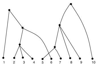
Figure 1: This forest represents the ${\mathcal{F}}_{G(1,1,10)}$-nested set ${\mathcal{S}}$ made by the irreducibles $\{2,3,4\}$, $\{2,3,4,6\}$, $\{1,2,3,4,6\}$, $\{5,7\}$, $\{5,7,8,9\}$, $\{5,7,8,9,10\}$.

One can show, using a bijection proven in [17] (see [26] for a variant), that there are actions of ‘big’ symmetric groups on the set of ${\mathcal{F}}_{G(1,1,n)}$-nested sets. Namely, the symmetric group $S_{n+k-1}$ acts on the set of the ${\mathcal{F}}_{G(1,1,n)}$-nested sets ${\mathcal{S}}$ such that $|{\mathcal{S}}|=k$ and ${\mathcal{S}}$ includes $\{1,2,...,n\}$. These actions can be extended to the basis of cohomology described in Theorem 2.2: in [4] (Theorem 10.1) it was shown that one can obtain, by counting the orbits of these actions, an exponential (not recursive) formula for a series that computes the Betti numbers of the models $Y_{G(1,1,n)}$.

As we mentioned in the Introduction, some recursive formulas for the Poincarè series of these varieties are well known (see for instance [33], [39], [24]).

Let us describe the formula obtained in [4], that is the starting point for our generalizations in the next sections. We denote by $\Psi(q,t,z)$ the following exponential generating series:

$$\Psi(q,t,z)=1+\sum_{n\geq 2,\;{\mathcal{S}}}P(S)z^{|{\mathcal{S}}|}\frac{t^{n+|{\mathcal{S}}|-1}}{(n+|{\mathcal{S}}|-1)!}$$

where, for every $n\geq 2$,

• ${\mathcal{S}}$ ranges over all the nested sets of the building set ${\mathcal{F}}_{G(1,1,n)}$;

• $P({\mathcal{S}})$ is the polynomial, in the variable $q$ (to be considered of degree 2), that expresses the contribution to $H^{*}(Y_{G(1,1,n)},{\mathbb{Z}})$ provided by all the monomials $m_{f}$ in the Yuzvinski basis such that $supp\ f={\mathcal{S}}$.

Theorem 3.1 (see [4], Theorem 10.1).

We have the following formula for the series $\Psi(q,t,z)$:

$$\Psi(q,t,z)=e^{t}\prod_{i\geq 3}e^{zq[i-2]_{q}\frac{t^{i}}{i!}}$$

where $[j]_{q}$ denotes the $q$-analog of $j$: $[j]_{q}=1+q+\cdots+q^{j-1}$.

Remark 3.1.

In [4] the result above is stated about the minimal projective De Concini-Procesi model, that is obtained starting from the projectivized hyperplane arrangement, but, as it was shown in [9], the integer homology rings of a model $Y_{\mathcal{G}}$ and of its corresponding projective model ${\overline{Y}}_{\mathcal{G}}$ are isomorphic.

Example 3.1.

In order to compute the Poincaré polynomial of $Y_{G(1,1,6)}$ from the formula above one has to single out all the monomials in $\Psi$ whose $z,t$ component is $t^{k}z^{s}$ with $k-s=5$. A product of the exponential functions that appear in the formula gives:

$$\frac{t^{5}}{5!}[1]+\frac{t^{6}}{6!}z[42q+22q^{2}+7q^{3}+q^{4}]+\frac{t^{7}}{7!}z^{2}[35q^{3}+105q^{2}]$$

Therefore the Poincaré polynomial of $Y_{G(1,1,6)}$, that is equal to the Poincaré polynomial of the moduli space ${\overline{M}}_{0,7}$, is $1+(42q+22q^{2}+7q^{3}+q^{4})+(35q^{3}+105q^{2})=1+42q+127q^{2}+42q^{3}+q^{4}$.

4 Extension to $G(r,1,n)$, $G(r,p,n)$ and $G(r,r,n)$

In this section we will describe the building sets of irreducibles associated to the groups $G(r,p,n)$, and their corresponding nested sets.

We notice that this combinatorial setting could be described also in the language of Dowling lattices: for instance, the intersection poset of the reflection arrangement of type $G(r,p,n)$ when $p<r$ is the Dowling lattice $Q_{n}({\mathbb{Z}}_{r})$ (see [16]), and we are considering its minimal building set and its nested set complex, according to the combinatorial definition of Feichtner and Kozlov in [21]. For this combinatorial approach, and for its further extensions to Bergman geometry, one could refer to [1], [2], [12], [20], [32]. In particular, in the first sections of [12] (and in Remark 4.7) one can find an useful overview on the many “bridges” between combinatorics and geometry related to this subject.

4.1 The building set of irreducibles

The reflecting hyperplanes of the arrangement in ${\mathbb{C}}^{n}$ associated with the full monoidal group $G(r,1,n)$ coincide with the reflecting hyperplanes of $G(r,p,n)$ when $p<r$ and have been described in the Introduction.

One can easily check that the building set of irreducibles ${\mathcal{F}}_{G(r,1,n)}$ (that is equal to ${\mathcal{F}}_{G(r,p,n)}$ when $p<r$) is made by two families of subspaces. The subspaces in the first family are the strong subspaces $\overline{H}_{i_{1},i_{2},...,i_{k}}$ (the adjective ‘strong’ comes from the analysis of the $B_{n}$ and $D_{n}$ case in [39]), that are the annihilators of the subspaces in ${\mathbb{C}}^{n}$ described by the equations

$$x_{i_{1}}=x_{i_{2}}=\cdots=x_{i_{t}}=0$$

where $1\leq t\leq n$. We can represent them by associating to $\overline{H}_{i_{1},i_{2},...,i_{t}}$ the subset $\{0,i_{1},i_{2},...,i_{t}\}$ of $\{0,1,...,n\}$. The second family is made by the weak subspaces, that are the annihilators $H_{i_{1},i_{2},...,i_{t}}(\alpha_{2},...,\alpha_{t})$ of the subspaces in ${\mathbb{C}}^{n}$ described by the equations:

$$x_{i_{1}}=\zeta^{\alpha_{2}}x_{i_{2}}=\cdots=\zeta^{\alpha_{t}}x_{i_{t}}$$

where $2\leq t\leq n$ and, for every $s$, $0\leq\alpha_{s}\leq r-1$.

Remark 4.1 (Notation).

Let us suppose that $i_{1}<i_{2}<\cdots<i_{t}$; then we can represent these weak subspaces by associating to $H_{i_{1},i_{2},...,i_{t}}(\alpha_{2},...\alpha_{t})$ the weighted subset $\{i_{1},\stackrel{{\scriptstyle\alpha_{2}}}{{i}}_{2},...,\stackrel{{\scriptstyle\alpha_{t}}}{{i}}_{t}\}$ of $\{1,...,n\}$. The weights are integers modulo $r$, and here (and in the sequel) if a weight is 0 we will omit to write it.

We observe that the building set of irreducibles ${\mathcal{F}}_{G(r,r,n)}$ can be obtained from ${\mathcal{F}}_{G(r,1,n)}$ by removing some strong subspaces, namely the hyperplanes $\overline{H}_{i}$, for every $i=1,...,n$. Moreover, if $r=2$, i.e. in the $D_{n}$ case, one needs to remove also the two dimensional subspaces $\overline{H}_{i,j}$. In fact we notice that the subspaces $\overline{H}_{i,j}$ are irreducible only if $r\geq 3$: since the $r$ lines $H_{i,j}(\alpha)$ (with $0\leq\alpha\leq r-1$) belong to ${\mathcal{F}}_{G(r,r,n)}$, when $r\geq 3$ it is not true that the two dimensional subspace $\overline{H}_{i,j}$ is the direct sum of the maximal subspaces of ${\mathcal{F}}_{G(r,r,n)}$ contained in it.

4.2 Nested sets for ${\mathcal{F}}_{G(r,1,n)}$ and ${\mathcal{F}}_{G(r,r,n)}$

The nested sets ${\mathcal{S}}=\{A_{1},...,A_{m}\}$ for ${\mathcal{F}}_{G(r,1,n)}$ or ${\mathcal{F}}_{G(r,r,n)}$, according to Definition 2.4, are characterized by the following properties:

• given any pair of subspaces $A_{i},A_{j}\in{\mathcal{S}}$, they are in direct sum or they are one included into the other;

• if there are strong subspaces in ${\mathcal{S}}$, they are linearly ordered by inclusion;

• a strong subspace is never included into a weak subspace.

According to the representation of the irreducibles by subsets of $\{0,1,....,n\}$ (more precisely, the subsets that do not contain 0 are weighted subsets) described in the preceding section, a nested set is represented by a set $\{A^{\prime}_{1},...,A^{\prime}_{m}\}$ of (possibly weighted) subsets of $\{0,...,n\}$ with the following properties:

• the subsets that contain 0 are not weighted; they are linearly ordered by inclusion;

• the subsets that do not contain 0 are weighted;

• for any pair of subsets $A^{\prime}_{i},A^{\prime}_{j}$, we have that, forgetting their weights, they are one included into the other or disjoint; if $A^{\prime}_{i},A^{\prime}_{j}$ both represent weak subspaces one included into the other (say $A^{\prime}_{i}\subset A^{\prime}_{j}$), then their weights must be compatible. Since we adopt for $A^{\prime}_{i}$ and $A^{\prime}_{j}$ the notation of Remark 4.1, this means that, up to the multiplication of all the weights of $A^{\prime}_{i}$ by the same power of $\zeta$, the weights associated to the same numbers must be equal.

We can represent a nested set by an oriented weighted forest as in Figure 2. Every internal vertex $v$ represents the subset obtained considering the leaves that belong to the subtree stemming from $v$. In particular, if $v$ is weak, it represents a weighted subset, in the following way. First of all, if a weak vertex is the root of a tree, we put its weight to be equal to 0 (so we don’t write it). Then, given any weak vertex $w$, the weight that one appends to the leaf $i$ in its associated weighted subset is given by the sum (modulo $r$) of the weights that one finds in the oriented connected path from $w$ to $i$ (we do not take into account the weight of $w$). According to the above described rules, there is a unique way to put the weights in the weighted forest respecting the notation of Remark 4.1.

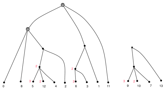
Figure 2: A nested set in the case $G(4,1,13)$. The ’big’ internal vertices represent the strong subspaces. The red numbers are the weights. The nested set represented in the picture is therefore made by the strong subspaces: $\{0,2,4,5,8,12\},\{0,1,2,3,4,5,6,8,11,12\}$ and by the weak subspaces $\{\stackrel{{\scriptstyle}}{{4}},\stackrel{{\scriptstyle{\color[rgb]{1,0,0}3}}}{{5}},\stackrel{{\scriptstyle{\color[rgb]{1,0,0}2}}}{{12}}\}$, $\{\stackrel{{\scriptstyle}}{{2}},\stackrel{{\scriptstyle{\color[rgb]{1,0,0}2}}}{{4}},\stackrel{{\scriptstyle{\color[rgb]{1,0,0}1}}}{{5}},\stackrel{{\scriptstyle}}{{12}}\}$, $\{\stackrel{{\scriptstyle}}{{3}},\stackrel{{\scriptstyle{\color[rgb]{1,0,0}2}}}{{6}}\}$, $\{\stackrel{{\scriptstyle}}{{1}},\stackrel{{\scriptstyle{\color[rgb]{1,0,0}2}}}{{3}},\stackrel{{\scriptstyle}}{{6}}\}$, $\{\stackrel{{\scriptstyle}}{{7}},\stackrel{{\scriptstyle{\color[rgb]{1,0,0}3}}}{{9}},\stackrel{{\scriptstyle{\color[rgb]{1,0,0}2}}}{{10}}\}$, $\{\stackrel{{\scriptstyle}}{{7}},\stackrel{{\scriptstyle{\color[rgb]{1,0,0}3}}}{{9}},\stackrel{{\scriptstyle{\color[rgb]{1,0,0}2}}}{{10}},\stackrel{{\scriptstyle}}{{13}}\}$.

5 Series

The results of Section 3 on the computation of Betti numbers of $Y_{G(1,1,n)}$ can be extended to the models $Y_{G(r,1,n)}$ ($=Y_{G(r,p,n)}$ when $p<r$) and $Y_{G(r,r,n)}$. Our goal is to give a non recursive formula for the Poincaré series

$$\Phi_{G(r,a)}(q,t)=1+\sum_{n\geq 2}Poin(Y_{G(r,a,n)})(q)\frac{t^{n}}{n!}$$

where $Poin(Y_{G(r,a,n)})(q)$ is the Poincaré polynomial of the model $Y_{G(r,a,n)}$.

We start by singling out the contribution to $\Phi_{G(r,a)}(q,t)$ given by the monomials of the Yuzvinski basis whose support does not contain strong subspaces. In terms of the Dowling lattice, the supports of these monomials are nested sets whose elements belong to the subposet $Q_{n}^{0}({\mathbb{Z}}^{r})$ of $Q_{n}({\mathbb{Z}}^{r})$ defined by Hultman in [32].

Definition 5.1.

Let $a=1$ or $a=r$ and let us denote by $K_{G(r,a)}(q,t,z)$ the following exponential generating series:

$$K_{G(r,a)}(q,t,z)=1+\sum_{n\geq 2,\;{\mathcal{S}}}P(S)z^{|{\mathcal{S}}|}\frac{t^{n+|{\mathcal{S}}|-1}}{(n+|{\mathcal{S}}|-1)!}$$

where, for every $n\geq 2$ (while $r$ remains fixed),

• ${\mathcal{S}}$ ranges over all the nested sets of the building set ${\mathcal{F}}_{G(r,a,n)}$ that do not contain strong subspaces;

• $P({\mathcal{S}})$ is the polynomial, in the variable $q$, that expresses the contribution to $H^{*}(Y_{{\mathcal{F}}_{G(r,a,n)}},{\mathbb{Z}})$ provided by all the monomials $m_{f}$ in the Yuzvinski basis such that $supp\ f={\mathcal{S}}$.

We notice that the series $K_{G(r,a)}(q,t,z)$ doesn’t change in the two cases $G(r,1,n)$ or $G(r,r,n)$, since only weak subspaces are involved.

Theorem 5.1.

We have the following formula for the series $K_{G(r,a)}(q,t,z)$ (when $a=1$ or $a=r$):

$$K_{G(r,a)}(q,t,z)=e^{t}\prod_{i\geq 3}e^{\frac{z}{r}q[i-2]_{q}\frac{(rt)^{i}}{i!}}$$

where $[j]_{q}$ denotes the $q$-analog of $j$: $[j]_{q}=1+q+\cdots+q^{j-1}$.

Proof.

This is a variant of Theorem 3.1, nevertheless we write the details of the proof for the convenience of the reader.

A monomial $m$ of the Yuzvinsky basis of $Y_{G(r,1,n)}$ can be represented by a weighted partition with exponents, in the following way. The support of the monomial is given, as we know from Theorem 2.2, by a ${\mathcal{F}}_{G(r,1,n)}$-nested set, and we are considering the monomials such that this nested set is made by weak subspaces.

For instance in $H^{*}(Y_{G(4,1,13)})$ the support of the monomial

$$c_{\{\stackrel{{\scriptstyle}}{{4}},\stackrel{{\scriptstyle{\color[rgb]{1,0,0}3}}}{{5}},\stackrel{{\scriptstyle{\color[rgb]{1,0,0}2}}}{{12}}\}}c^{2}_{\{\stackrel{{\scriptstyle}}{{2}},\stackrel{{\scriptstyle{\color[rgb]{1,0,0}2}}}{{4}},\stackrel{{\scriptstyle{\color[rgb]{1,0,0}1}}}{{5}},8,11,\stackrel{{\scriptstyle}}{{12}}\}}c_{\{\stackrel{{\scriptstyle}}{{7}},\stackrel{{\scriptstyle{\color[rgb]{1,0,0}3}}}{{9}},\stackrel{{\scriptstyle{\color[rgb]{1,0,0}2}}}{{10}}\}}c^{3}_{\{1,3,6,\stackrel{{\scriptstyle}}{{7}},\stackrel{{\scriptstyle{\color[rgb]{1,0,0}3}}}{{9}},\stackrel{{\scriptstyle{\color[rgb]{1,0,0}2}}}{{10}},\stackrel{{\scriptstyle}}{{13}}\}}$$

is described by the weighted forest in Figure 3.

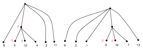
Figure 3: This weighted forest represents the support of the monomial $c_{\{\stackrel{{\scriptstyle}}{{4}},\stackrel{{\scriptstyle{\color[rgb]{1,0,0}3}}}{{5}},\stackrel{{\scriptstyle{\color[rgb]{1,0,0}2}}}{{12}}\}}c^{2}_{\{\stackrel{{\scriptstyle}}{{2}},\stackrel{{\scriptstyle{\color[rgb]{1,0,0}2}}}{{4}},\stackrel{{\scriptstyle{\color[rgb]{1,0,0}1}}}{{5}},8,11,\stackrel{{\scriptstyle}}{{12}}\}}c_{\{\stackrel{{\scriptstyle}}{{7}},\stackrel{{\scriptstyle{\color[rgb]{1,0,0}3}}}{{9}},\stackrel{{\scriptstyle{\color[rgb]{1,0,0}2}}}{{10}}\}}c^{3}_{\{1,3,6,\stackrel{{\scriptstyle}}{{7}},\stackrel{{\scriptstyle{\color[rgb]{1,0,0}3}}}{{9}},\stackrel{{\scriptstyle{\color[rgb]{1,0,0}2}}}{{10}},\stackrel{{\scriptstyle}}{{13}}\}}$ in $H^{*}(Y_{G(4,1,13)})$.

Then, following [26], we can label the internal vertices of the forest as in Figure 4: we put labels level by level, and the label of a vertex $v$ is less than the label of a vertex $w$ iff the subtree that stems from $v$ contains a leaf whose label is smaller than the labels of all the leaves in the subtree that stems from $w$. If the forest has more than one connected component (as in Figure 4), we add an extra vertex on top, with the maximum label.

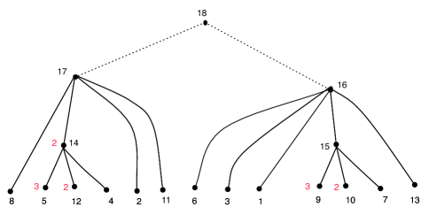
Figure 4: We can label (level by level) the internal vertices of the forest of Figure 3 with the numbers $14,15,16,17$. Since the forest is not connected, we add a vertex on top, with the maximum label $18$.

We can then associate to the support of the monomial $m$ a weighted partition, by looking at the internal vertices of the labelled forest and taking into account, for each internal vertex, the labels and weights of the vertices covered by it. For instance, looking at the weighted forest represented in Figure 4, we associate to it the the weighted partition:

$$\{\stackrel{{\scriptstyle}}{{4}},\stackrel{{\scriptstyle{\color[rgb]{1,0,0}3}}}{{5}},\stackrel{{\scriptstyle{\color[rgb]{1,0,0}2}}}{{12}}\}\{\stackrel{{\scriptstyle}}{{2}},8,11,\stackrel{{\scriptstyle{\color[rgb]{1,0,0}2}}}{{14}}\}\{\stackrel{{\scriptstyle}}{{7}},\stackrel{{\scriptstyle{\color[rgb]{1,0,0}3}}}{{9}},\stackrel{{\scriptstyle{\color[rgb]{1,0,0}2}}}{{10}}\}\{1,3,6,\stackrel{{\scriptstyle}}{{13}},15\},\{16,17\}$$

Finally we can associate to the monomial

$$c_{\{\stackrel{{\scriptstyle}}{{4}},\stackrel{{\scriptstyle{\color[rgb]{1,0,0}3}}}{{5}},\stackrel{{\scriptstyle{\color[rgb]{1,0,0}2}}}{{12}}\}}c^{2}_{\{\stackrel{{\scriptstyle}}{{2}},\stackrel{{\scriptstyle{\color[rgb]{1,0,0}2}}}{{4}},\stackrel{{\scriptstyle{\color[rgb]{1,0,0}1}}}{{5}},8,11,\stackrel{{\scriptstyle}}{{12}}\}}c_{\{\stackrel{{\scriptstyle}}{{7}},\stackrel{{\scriptstyle{\color[rgb]{1,0,0}3}}}{{9}},\stackrel{{\scriptstyle{\color[rgb]{1,0,0}2}}}{{10}}\}}c^{3}_{\{1,3,6,\stackrel{{\scriptstyle}}{{7}},\stackrel{{\scriptstyle{\color[rgb]{1,0,0}3}}}{{9}},\stackrel{{\scriptstyle{\color[rgb]{1,0,0}2}}}{{10}},\stackrel{{\scriptstyle}}{{13}}\}}$$

the following weighted partition of $\{1,...,17\}$ with exponents attached to the parts, in order to keep into account the exponents in the monomial:

$$\{\stackrel{{\scriptstyle}}{{4}},\stackrel{{\scriptstyle{\color[rgb]{1,0,0}3}}}{{5}},\stackrel{{\scriptstyle{\color[rgb]{1,0,0}2}}}{{12}}\}\{\stackrel{{\scriptstyle}}{{2}},8,11,\stackrel{{\scriptstyle{\color[rgb]{1,0,0}2}}}{{14}}\}^{2}\{\stackrel{{\scriptstyle}}{{7}},\stackrel{{\scriptstyle{\color[rgb]{1,0,0}3}}}{{9}},\stackrel{{\scriptstyle{\color[rgb]{1,0,0}2}}}{{10}}\}\{1,3,6,\stackrel{{\scriptstyle}}{{13}},15\}^{3}\{16,17\}^{0}$$

Remark 5.1.

This process, if applied to a forest with more then one connected component, adds an extra vertex on top. In this case we obtain a part with exponent 0, like $\{16,17\}^{0}$ in the example above. We notice that this part, by construction, contains 17, the maximum of $\{1,2,...,17\}$.

Going back to our proof, let us denote by ${\mathcal{B}}(r,1)_{weak}$ the set of all the Yuzvinski basis monomials of all the models $Y_{G(r,1,n)}$ ($n\geq 3$) whose support is made by weak subsets. As we remarked above, we can think of these monomials as weighted partitions with exponents attached to the parts. Let us now denote by ${\mathcal{P}}(r,1)$ the union, for every $j\geq 3$, of the set of weighted partitions of $\{1,..,j\}$ with exponents, such that:

• at most one of the parts has exponent equal to 0 (and cardinality $\geq 2$). If this part exists, it contains the maximum number $j$;

• the other parts $I$ have cardinality $\geq 3$ and their exponent $\alpha_{I}$ satisfies $1\leq\alpha_{I}\leq|I|-2$.

As an easy corollary of Theorem 2.1 in [26], we know that the above described map from ${\mathcal{B}}(r,1)_{weak}$ to ${\mathcal{P}}(r,1)$ is bijective, therefore we can find a formula for $K_{G(r,a)}(q,t,z)$ by counting the contribution of all the elements of ${\mathcal{P}}(r,1)$.

Then we single out the contribution given to $K_{G(r,a)}(q,t,z)$ by all the parts represented by subsets with cardinality $i\geq 3$ and with nonzero exponent. If in a weighted partition there is only one such part its contribution is $\frac{z}{r}(q+q^{2}+\cdots+q^{i-2})\frac{(rt)^{i}}{i!}$. If there are $j$ such parts the associated contribution is $(\frac{z}{r})^{j}(q+q^{2}+\cdots+q^{i-2})^{j}\frac{(\frac{(rt)^{i}}{i!})^{j}}{j!}$. In conclusion the contribution of all the parts represented by subsets with cardinality $i\geq 3$ and with nonzero label is provided by

$$e^{\frac{z}{r}(q+q^{2}+\cdots+q^{i-2})\frac{(rt)^{i}}{i!}}-1$$

Let us now focus on the contribution to $K_{G(r,a)}(q,t,z)$ that comes from the parts with cardinality $i\geq 2$ and with exponent equal to 0. For every monomial in the basis there is at most one such part (that must contain the highest number of the set that we are partitioning), and its contribution is $\frac{t^{i-1}}{(i-1)!}$. We note that by construction all the weights of the numbers that belong to this part are equal to 0, since it does not represent a subspace in the support of the monomial.

The total contribution of the elements with exponent equal to 0 is therefore $\sum_{i\geq 2}\frac{t^{i-1}}{(i-1)!}$. Summing up, we observe that the expression

$$e^{t}\prod_{i\geq 3}e^{\frac{z}{r}q[i-2]_{q}\frac{(rt)^{i}}{i!}}$$

allows us to take into account the contribution to $K_{G(r,a)}(q,t,z)$ of all the elements in ${\mathcal{P}}(r,1)$. ∎

5.1 Series for $G=G(r,1,n)$

Let us now find a formula for the Poincaré series $\Phi_{G(r,1)}(q,t)$ of the models $Y_{G(r,1,n)}$.

In this case the support of a monomial of the Yuzvinsky basis can be represented by a forest that has a shape like the one suggested in Figure 5.

There may be at most one connected component with strong vertices. Then the strong vertices, as in the picture, form a chain, and below each of them there is a subgraph made by weak vertices. There may be other connected components that are made by weak vertices.

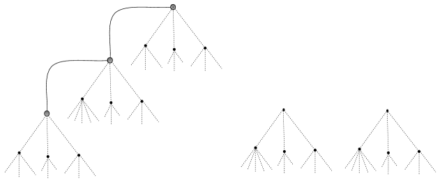
Figure 5: The shape of a forest that represents the support of a basis monomial of $H^{*}(Y_{G(r,1,n)})$. There is at most one component with strong vertices. Then the strong vertices, as in the picture, form a chain, and below each of them there is a subgraph made by weak vertices. There may be other connected components that are made by weak vertices.

The following series will play a key role in computing the contribution of a weak subtree that stems from a strong vertex:

$$\gamma_{G(r,1)}(q,t,z)=\left(\sum_{i\geq 2}\frac{t^{i-1}}{(i-1)!}q[i-1]_{q}\right)\prod_{i\geq 3}e^{q[i-2]_{q}\frac{z}{r}\left(\frac{tr}{i!}\right)^{i}}$$

The idea is that we can evaluate the series $\gamma_{G(r,1)}(q,t,z)$ in $z=\frac{\partial}{\partial t}$ and then integrate (formally, with constant equal to 0) with respect to the variable $t$. As a result we get a new series in the variables $q,t$ which we denote by $\Gamma_{G(r,1)}(q,t)$:

$$\Gamma_{G(r,1)}(q,t)=\int\gamma_{G(r,1)}(q,t,\frac{\partial}{\partial t})$$

Remark 5.2.

Here and in the sequel, when we say that we evaluate a series in $z=\frac{\partial}{\partial t}$, we mean that first we compute the series, then, in every monomial that appears in the final expression of the series, we put $z=\frac{\partial}{\partial t}$.

At the same way we define

$${\mathcal{K}}_{G(r,1)}(q,t)=1+\int K_{G(r,1)}(q,t,\frac{\partial}{\partial t})$$

Theorem 5.2.

We have the following formula for the Poincaré series of the models $Y_{G(r,1,n)}$:

$$\Phi_{G(r,1)}(q,t)=\frac{1}{1-\Gamma_{G(r,1)}(q,t)}{\mathcal{K}}_{G(r,1)}(q,t)$$

Proof.

First we observe that

$${\mathcal{K}}_{G(r,1)}(q,t)=1+\int K_{G(r,1)}(q,t,\frac{\partial}{\partial t})=1+t+\sum_{n\geq 2,\;{\mathcal{S}}\ weak}P(S)\frac{t^{n}}{n!}=1+t+\sum_{n\geq 2}Poin^{w}(Y_{G(r,1,n)})(q)\frac{t^{n}}{n!}$$

where ${\mathcal{S}}\ weak$ means that we are considering only the nested sets made by weak subspaces, and $Poin^{w}(Y_{G(r,1,n)})(q)$ is the contribution to the Poincaré polynomial of the model $Y_{G(r,1,n)}$ given by the basis monomials whose nested set is ‘weak’.

Then we observe that the difference between the series $\gamma_{G(r,1)}(q,t,z)$ and $K_{G(r,1)}(q,t,z)$ consists only in the first exponential factor, where we find $\sum_{i\geq 2}\frac{t^{i-1}}{(i-1)!}q[i-1]_{q}$ instead than $\sum_{i\geq 2}\frac{t^{i-1}}{(i-1)!}$: the $q$-polynomial $q[i-1]_{q}$ counts the contribution to the Poincarè series given by a strong vertex which covers $i$ weak vertices in the graph. The evaluation of $z$ as $\frac{\partial}{\partial t}$ and the integral transform $\gamma_{G(r,1)}(q,t,z)$ into $\Gamma_{G(r,1)}(q,t)$, that gives the correct contribution to the Poincaré series of a strong vertex and of the weak subgraph stemming from it.

Since the strong vertices are linearly ordered, if there are $m$ strong vertices their contribution is given by $\Gamma_{G(r,1)}(q,t)^{m}$, so the total contribution of strong vertices to $\Phi_{G(r,1)}(q,t)$ is

$$\Gamma_{G(r,1)}(q,t)+\Gamma_{G(r,1)}(q,t)^{2}+\Gamma_{G(r,1)}(q,t)^{3}+...$$

Multiplying by ${\mathcal{K}}_{G(r,1)}(q,t)$ we take into account the contributions of the components of the forest that don’t have strong vertices, and this proves our claim.

∎

5.2 Series for $G=G(r,r,n)$

Theorem 5.3.

When $r\geq 3$, the series $\Phi_{G(r,r)}(q,t)$ coincides with $\Phi_{G(r,1)}(q,t)$. When $r=2$ (i.e. the $D_{n}$ case), we have

$$\Phi_{G(2,2)}(q,t)=\frac{(1-q\frac{t^{2}}{2})}{1-\Gamma_{G(2,1)}(q,t)}{\mathcal{K}}_{G(2,1)}(q,t)$$

Proof.

When $r=2$, the only modification we have with respect to the computation of Theorem 5.2 is that among the forests that represent the supports of the monomials we do not have forests whose lower strong vertex corresponds to a two dimensional subspace $\overline{H}_{i,j}$. The contribution to $\Phi_{G(2,1)}(q,t)$ of the associated monomials is computed by the series

$$\frac{q\frac{t^{2}}{2}}{1-\Gamma_{G(2,1)}(q,t)}{\mathcal{K}}_{G(2,1)}(q,t)$$

so we have to subtract it from $\Phi_{G(2,1)}(q,t)$. ∎

6 Real spherical models

When the group $G$ is real we can construct a spherical model associated to it, as a special case of a construction in [25].

Let us consider the real arrangement ${\mathcal{A}}_{G}$ given in the euclidean space $V$ by the reflecting hyperplanes of $G$, and let us identify $V^{*}$ with $V$ by the scalar product. Therefore the subspaces in the minimal building set, that we denote by ${\mathcal{F}}_{G}$, are identified with subspaces in $V$. We will denote by ${\mathcal{M}}(G)$ the complement of the arrangement ${\mathcal{A}}_{G}$ in $V$.

Moreover, we denote by $S(V)$ the unit sphere in $V$, and, for every subspace $A\subset V$, let $S(A)=A\cap S(V)$. Let us consider the compact manifold

$$K=S(V)\times\prod_{A\in{\mathcal{F}}_{G}}S(A)$$

There is an open embedding $\phi:\>{\mathcal{M}}(G)/{\mathbb{R}}^{+}\longrightarrow K$ which is obtained as a composition of the section $s:\>{\mathcal{M}}(G)/{\mathbb{R}}^{+}\mapsto{\mathcal{M}}(G)$

$$s([p])=\frac{p}{|p|}\in S(V)\cap{\mathcal{M}}(G)$$

with the map

$${\mathcal{M}}(G)\mapsto S(V)\times\prod_{A\in{\mathcal{F}}_{G}}S(A)$$

that is given by the normalization on the first factor and by the orthogonal projections followed by normalizations on the other factors.

Definition 6.1.

We denote by $CY_{G}$ the closure in $K$ of $\phi({\mathcal{M}}(G)/{\mathbb{R}}^{+})$.

It turns out that $CY_{G}$ is a smooth manifold with corners that has as many connected components as the number of chambers of the arrangement.

A linear realization of $CY_{G}$ as a disjoint union of polytopes has been constructed in [27]. The polytopes involved lie inside the chambers of the arrangement: in the fundamental chamber we find the graph associahedron $P_{G}$ of type $G$ (i.e. the graph polytope defined in [15] and [6] associated with the Dynkin graph of type $G$) and in the other chambers there is the image of this polytope via the action of $G$. The faces of the graph associahedron $P_{G}$ that lies in the fundamental chamber are parametrized by the fundamental nested sets defined as follows. Given a basis of simple roots for the root system of $G$, the fundamental building set of irreducibles is the set of irreducible subspaces that are spanned by simple roots. The nested sets associated to this building set are the fundamental nested sets.

Now, as it is well known, the chambers of the arrangement are in bijection with the elements of $G$. It follows that the faces of the graph associahedra that are the components of $CY_{G}$ are parametrized by pairs $(w,{\mathcal{S}}^{\prime})$ where $w\in G$ and ${\mathcal{S}}^{\prime}$ is a fundamental nested set.

From Section 5 of [25] we know that there is a natural projection map ${\mathcal{P}}$ from $CY_{G}$ to ${\overline{Y}}_{{\mathcal{F}}_{G}}$, the real compact wonderful model associated with the group $G$. This model is constructed in [9] as the closure of the image of the map

$${\mathbb{P}}({\mathcal{M}}(G))\longrightarrow{\mathbb{P}}(V)\times\prod_{A\in{\mathcal{F}}_{G}}{\mathbb{P}}(A)$$

where we identify the euclidean space $V$ with its dual as above.

Then Theorem 5.2 of [25] states that ${\mathcal{P}}$ is $2^{k+1}\rightarrow 1$ when restricted to the open parts of the boundary components of codimension $k$ of $CY_{G}$. Therefore ${\overline{Y}}_{{\mathcal{F}}_{G}}$ can be obtained by glueing $|G|$ copies of the polytope $P_{G}$ in a prescribed way.

7 Counting faces of polytopes in the real cases

A variant of the computation of the Poincaré series of the model $Y_{G}$ allows us to find a series that counts the number of faces of $CY_{G}$. From this one immediately obtains formulas for the number of faces of the graph associahedron $P_{G}$.

7.1 Case $A_{n-1}$, group $S_{n}=G(1,1,n)$.

When $G=S_{n}$, i.e. when we are dealing with the arrangement of type $A_{n-1}$, the polytope $P_{G}$ is a $n-2$ dimensional Stasheff’s associahedron. The entries of the $f-$vectors of these associahedra are the well known Kirkman-Cayley numbers. Anyway, in order to ‘test’ our method, in this section we show how we can obtain a series that encodes all the information about the $f$-vectors of the Stasheff’s associahedra.

First we notice that every nested set in ${\mathcal{F}}_{G(1,1,n)}$ is represented by a tree on $n$ leaves, as we explained in Section 3. Let us now consider planar pictures of these trees, adding an ordering condition on the leaves: even if two trees represent the same nested set, we consider them as different objects if the order from left to right of their leaves is different. Each of these plane trees represents a face of $CY_{G(1,1,n)}$: the plane trees where the leaves, from left to right, form the list $1,2,..,n$ represent the fundamental nested sets, so the trees whose leaves form the list $w(1),w(2),...,w(n)$ (where $w\in S_{n}$) describe the faces $(w,{\mathcal{S}}^{\prime})$ of the polytope that lies in the chamber corresponding to $w$.

In conclusion, the faces of the disjoint union of polytopes $CY_{G(1,1,n)}$ are in bijective correspondence with the set of the above described plane rooted trees on $n$ ordered leaves.

Definition 7.1.

Let us denote by $F(z,t)$ the series

$$F(z,t)=\sum_{n\geq 2}\sum_{T}z^{s(T)}\frac{t^{n+s(T)-1}}{(n+s(T)-1)!}$$ (1)

where $T$ ranges over all the above described plane rooted trees with $n$ ordered leaves and $s(T)$ is the number of internal vertices in $T$.

We observe that we can write

$$F(z,t)=\sum_{n\geq 2,1\leq s\leq n-1}\frac{C_{n,s}}{(n+s-1)!}z^{s}t^{n+s-1}$$

where $C_{n,s}$ is the number of $(s-1)$-codimensional faces of $CY_{G(1,1,n)}$. Therefore, the coefficient in $F(z,t)$ of $z^{s}t^{n+s-1}$ multiplied by $\frac{(n+s-1)!}{n!}$ is equal to the number of $(s-1)$-codimensional faces of the $n-2$ dimensional Stasheff’s associahedron, that is the Kirkman-Cayley number

$$D_{n+1,s-1}=\frac{1}{s}\binom{n-2}{s-1}\binom{n+s-1}{s-1}$$

Proposition 7.1.

We have $F(z,t)=e^{z\frac{t^{2}}{1-t}}-1$.

Proof.

As in the proof of Theorem 5.1 we want to count partitions of $\{1,...,n+k-1\}$ into $k$ parts with cardinality $\geq 2$ instead than plane trees with $n$ ordered leaves and $k$ internal vertices. An important difference is that here the order of the leaves is relevant; this can be translated in terms of partitions by considering partitions where each part is internally ordered. In fact an “ordered” variant of the bijection described in Section 5 (see Theorem 2.2 of [26]) associates to such a partition a tree on $n$ ordered leaves, as illustrated by Figure 6.

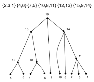
Figure 6: The internally ordered partition of $[1,15]$ into 6 blocks that is on top of the picture (the internal orderings are obtained reading from left to right), produces the rooted tree with 10 ordered leaves on the bottom of the picture. For every internal vertex $v$, the labels of the vertices and leaves covered by it, read from left to right, reproduce the internal orderings of a set of the partition.

Furthermore, in this case all the parts have exponent equal to 1 (in particular there is no part with exponent 0), and the parts have cardinality $\geq 2$.

When we single out the contribution given to $F(z,t)$ by all the parts represented by subsets with cardinality $i\geq 2$ we observe that if in a partition there is only one such part its contribution is $zt^{i}$ and if there are $j$ such parts their contribution is $z^{j}\frac{(t^{i})^{j}}{j!}$. The formula follows.

∎

Let us now consider the series

$$X(t)=\sum_{n\geq 2}\chi({\overline{Y}}_{G(1,1,n)})\frac{t^{n-1}}{(n-1)!}$$

where $\chi(\quad)$ denotes the Euler characteristic. There are several different ways to compute this series and a closed formula for $\chi({\overline{Y}}_{\mathcal{F}_{G(1,1,n)}})$ has been provided in [14] and [31]. Anyway we remark that we can compute $X(t)$ also from $F(z,t)$:

Corollary 7.1.

The series $X(t)$ can be obtained from the series $e^{\frac{z}{2}\frac{t^{2}}{1+t}}-1$ by evaluating $z$ as $\frac{\partial}{\partial t}$.

Proof.

We can compute the Euler characteristic by counting the faces of the $CW$ complex that covers ${\overline{Y}}_{\mathcal{F}_{\mathcal{A}_{n-1}}}$ according to the map ${\mathcal{P}}$ described in the end of Section 6. Then $e^{\frac{z}{2}\frac{t^{2}}{1+t}}-1$ is $F(\frac{z}{2},-t)$: the substitution $z\rightarrow\frac{z}{2}$ in $F(z,t)$ takes into account the $2^{k+1}\rightarrow 1$ glueings of the $k$-codimensional boundary components of $CY_{G(1,1,n)}$, while the substitution $t\rightarrow-t$ gives the correct sign $(-1)^{n-1+s}(=(-1)^{n-1-s})$ to the $(s-1)$-codimensional cells of the $CW$ complex.

∎

7.2 Cases $B_{n}$, group $G(2,1,n)$ and $D_{n}$, group $G(2,2,n)$.

Let us consider $a=1$ or $a=2$ and define the series

$$F_{CY_{G(2,a)}}(w,t)=\sum_{n}\sum_{1\leq j\leq n}C_{G(2,1),j}w^{j}\frac{t^{n}}{n!}$$

where $C_{G(2,a,n),j}$ is the number of $(j-1)$-codimensional faces of $CY_{G(2,a,n)}$. In view of the description of fundamental nested sets, and of the parametrization by pairs $(w,{\mathcal{S}}^{\prime})$ of the faces of $CY_{G(2,a,n)}$, this number coincides with the number of plane rooted weighted trees on $n+1$ leaves labelled by $\{0,1,...,n\}$ and ordered from left to right with the following properties (see Figure 7):

• the vertices may be weak or strong; the root is a strong vertex, and the strong vertices are linearly ordered;

• the leaves belong to a horizontal line; the first leaf on the left is the leaf 0, that is contained in the subgraph that stems from every strong vertex; the other leaves are put on the line in any order from left to right;

• there are at least two edges that go down from every internal vertex; in the $D_{n}$ case, i.e. if $a=2$, there must be at least four edges that go down from the lower strong vertex.

• there are weights 0 or 1 attached to the leaves and vertices, with the following restrictions: the root has weight 0 and when a vertex covers some other objects (where with ‘object’ we mean a vertex or a leaf), the leftmost object has weight 0. Furthermore, let us say that a leaf has parity 0 or 1 if the sum (modulo 2) of the weights that one finds in the path from the leaf to the root is 0 or 1 respectively; then, in the $D_{n}$ case the number of leaves with parity 1 must be even.

• in the $D_{n}$ case, the first leaf on the right of the leaf 0 may be equipped with and extra label ($+$, $-$ or $\pm$). More precisely, it has this extra label if it is covered by a weak vertex, with the following meaning: let $c$ be the label of the leaf on the right of $b$, then if in the subspace represented by the weak vertex there is the root $x_{c}+x_{b}$ we put the label $+$, if there is the root $x_{c}-x_{b}$ we put the label $-$. We also allow the following special case: there is a weak vertex that covers exactly two leaves, namely the leaf $b$ with the extra label $\pm$ and the leaf $c$; this notation means that in the nested set there are both the one dimensional subspaces spanned by the roots $x_{c}+x_{b}$ and $x_{c}-x_{b}$.

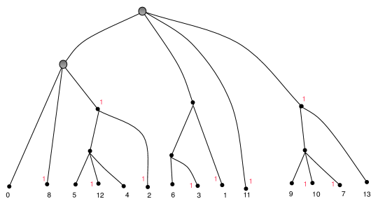
Figure 7: A valid plane oriented rooted tree that represents a face of codimension 7 of $CY_{G(2,1,13)}$.

Remark 7.1.

We notice that the combined information provided by the ordering from left to right of the leaves and by the weights of these trees determines the chamber of the arrangement that we are considering, since the chambers are in bijective correspondence with the orderings of the numbers $\{1,2,...,n\}$, with weights $0$ or $1$ attached to these numbers (these weights are recovered from the weights of a tree by attaching to a leaf its parity 0 or 1).

When $a=1$, i.e. in the $B_{n}$ case, the associated polytope is again the $(n-1)$-dimensional Stasheff’s associahedron whose $f$-vector is well known. Nevertheless we show a formula for $F_{CY_{G(2,1)}}(w,t)$ from which we will obtain a formula for $F_{CY_{G(2,2)}}(w,t)$. We remark that since $CY_{G(2,2,n)}$, for every $n$, is the disjoint union of $2^{n-1}n!$ polytopes, this immediately gives a formula that computes the $f$-vectors of the graph associahedra of type $D_{n}$.

One defines

$${\widetilde{\gamma}}_{G(2,1)}(t,z,w)=2\left(\sum_{i\geq 1}i(2t)^{i-1}\right)\prod_{j\geq 2}e^{\frac{wz}{2}\left(2t\right)^{j}}$$

This series plays the same role of the series $\gamma_{G(r,1)}$ in Section 5.1: it counts the contribution to $F_{CY_{G(2,1)}}(w,t)$ of the vertices of the weak subgraph that stems from a strong vertex (the leaves are considered weak except for the leaf 0). In this case, for a technical reason that will become clear later, there are two variables, $w$ and $z$, that count the same quantity, i.e. the number of internal vertices of this subgraph. As in the $G(1,1,n)$ case, the order from left to right of the leaves is relevant and therefore we are considering partitions into internally ordered parts. This time there are also weights, equal to 0 or 1, attached to each number of the partition.

The factor $2\left(\sum_{i\geq 1}i(2t)^{i-1}\right)$ has the following meaning: in a given partition there is a part, say of cardinality $i$, that contains the highest number, and represents the vertices connected by an arc to the strong vertex; then the contribution of this part is given by $2^{i}it^{i-1}$, where the factor $i$ counts the choices of the position of the highest number.

To obtain the exact contribution of the vertices of the weak subgraph that lies below a strong vertex, we have to pass from $\gamma_{G(r,1)}$ to the following series:

$${\widetilde{\Gamma}}_{G(2,1)}(t,w)=\int{\widetilde{\gamma}}_{G(2,1)}(t,\frac{\partial}{\partial t},w)$$

where the substitution of $z$ with $\frac{\partial}{\partial t}$ is performed as specified in Remark 5.2. We observe that the variable $w$ still counts the internal vertices of the subgraph.

Theorem 7.1.

We have

$$F_{CY_{G(2,1)}}(w,t)=\frac{1}{1-w{\widetilde{\Gamma}}_{G(2,1)}(t,w)}$$

Proof.

We have already discussed the meaning of the series ${\widetilde{\Gamma}}_{G(2,1)}(t,w)$. So, since the strong vertices are linearly ordered, the series $F_{CY_{G(2,1)}}(w,t)$ is equal to

$$w{\widetilde{\Gamma}}_{G(2,1)}(t,w)+(w{\widetilde{\Gamma}}_{G(2,1)}(t,w))^{2}+(w{\widetilde{\Gamma}}_{G(2,1)}(t,w))^{3}+...$$

∎

Example 7.1.

A simple computation shows that the first terms of the series $w{\widetilde{\Gamma}}_{G(2,1)}(t,w)$ are as follows:

$$w{\widetilde{\Gamma}}_{G(2,1)}(t,w)=w2t+(w^{2}+w)2^{2}t^{2}+(2w^{3}+3w^{2}+w)2^{3}t^{3}+(5w^{4}+10w^{3}+6w^{2}+w)2^{4}t^{4}+...$$

As a consequence, the first terms of $F_{CY_{G(2,1)}}(w,t)$ are:

$$F_{CY_{G(2,1)}}(w,t)=1+w2t+(2w^{2}+w)2^{2}t^{2}+(5w^{3}+5w^{2}+w)2^{3}t^{3}+(14w^{4}+21w^{3}+9w^{2}+w)2^{4}t^{4}+...$$

The coefficients that appear inside the parentheses give, as expected, the $f$-vectors of Stasheff’s associahedra.

We can now quickly obtain a formula in the $D_{n}$ case

Theorem 7.2.

We have

$$F_{CY_{G(2,2)}}(w,t)=\frac{(1-t)w{\widetilde{\Gamma}}_{G(2,1)}(t,w)-2tw-2t^{2}w-2t^{2}w^{2}}{1-w{\widetilde{\Gamma}}_{G(2,1)}(t,w)}$$

In particular, when $n\geq 4$, the coefficient of $w^{s}t^{n}$ of this series, divided by $2^{n-1}$, gives the number of faces of codimension $s-1$ of the $(n-1)$-dimensional associahedron of type $D$.

Proof.

A first difference with respect to the computation in the $B_{n}$ case is that we have to remove all the graphs such that the subgraph that stems from the lower strong vertex has only two or three leaves, namely the leaf 0 plus one or two leaves. A subgraph of this type that has only two leaves gives the contribution $2wt$ to ${\widetilde{\Gamma}}_{G(2,1)}(t,w)$, while if it has three leaves it gives the contribution $4(w+w^{2})t^{2}$ to ${\widetilde{\Gamma}}_{G(2,1)}(t,w)$. Furthermore, we have to take into account the extra label $+$, $-$ or $\pm$ of the leaf on the right of the leaf $0$ (we will call it the leaf $b$): this extra label appears only when the leaf $b$ is covered by a weak vertex. So in order to compute the contributions of the extra labels $+$ and $-$ we multiply by two the contribution of lower strong vertices computed so far:

$$2[w{\widetilde{\Gamma}}_{G(2,1)}(t,w)-2tw-2^{2}t^{2}(w+w^{2})]$$

and then subtract from it the contribution of lower strong vertices where the leaf $b$ is not covered by a weak vertex:

$$2[w{\widetilde{\Gamma}}_{G(2,1)}(t,w)-2tw-2^{2}t^{2}(w+w^{2})]-2t[w{\widetilde{\Gamma}}_{G(2,1)}(t,w)-2wt]$$

Then we add $2^{2}t^{2}w^{2}$ to take into account the case where the extra label $\pm$ appears. Finally, we obtain the following formula that computes the contribution of lower strong vertices:

$$\frac{1}{2}\left(2[w{\widetilde{\Gamma}}_{G(2,1)}(t,w)-2tw-2^{2}t^{2}(w+w^{2})]-2t[w{\widetilde{\Gamma}}_{G(2,1)}(t,w)-2wt]+2^{2}t^{2}w^{2}\right)$$

The factor $\frac{1}{2}$ takes into account that in the $D_{n}$ case we are considering only the trees where an even number of leaves have parity 1.

The contribution of strong vertices different from the lower one is computed dividing the formula that we have obtained by $1-w{\widetilde{\Gamma}}_{G(2,1)}(t,w)$. ∎

Example 7.2.

If one computes $F_{CY_{G(2,2)}}(w,t)$ from the formula above, starting from the formula for the first terms of $w{\widetilde{\Gamma}}_{G(2,1)}(t,w)$ shown in Example 7.1, one obtains that the coefficient of $2^{3}t^{4}$ in $F_{CY_{G(2,2)}}(w,t)$ is equal to:

$$16w^{4}+24w^{3}+10w^{2}+w$$

The coefficients that appear above give the $f$ vector of the graph associahedron of type $D_{4}$. We notice that a formula for the number of the vertices of these graph associahedra (in terms of the Catalan numbers) is provided by Proposition 5.4 of [35].

We notice that the coefficient of $2^{2}t^{3}$ in $F_{CY_{G(2,2)}}(w,t)$ is $5w^{3}+5w^{2}+w$, giving the $f$-vector of the $2$-dimensional Stasheff’s associahedron. This reflects the fact that the ‘degenerate’ root system $D_{3}$ is equal to $A_{3}$.

As a corollary of the results above, we can describe a series that computes the Euler characteristic of the real compact models of type $B_{n}$ and $D_{n}$ (closed formulas can be found in [31]):

Corollary 7.2.

For $a=1$ or $a=2$, if we evaluate the series $F_{CY_{G(2,a)}}(w,-t)$ in $w=-\frac{1}{2}$ we obtain the series

$$X_{CY_{G(2,a)}}(w,t)=\sum_{n}\sum_{1\leq j\leq n}\chi({\overline{Y}}_{G(2,a,n)})\frac{t^{n}}{n!}$$

that computes the Euler characteristic of the real compact models ${\overline{Y}}_{G(2,a,n)}$.

Proof.

This is an immediate consequence of the properties of the map ${\mathcal{P}}$, in particular of the $2^{k+1}\rightarrow 1$ glueings of the $k$-codimensional boundary components of $CY_{G(2,a)}$. ∎

References

- [1] Ardila, F., and Klivans, C. J. The Bergman complex of a matroid and phylogenetic trees. J. Combin. Theory Ser. B 96, 1 (2006), 38–49.
- [2] Ardila, F., Reiner, V., and Williams, L. Bergman complexes, Coxeter arrangements, and graph associahedra. Sém. Lothar. Combin. 54A (2005/07), Art. B54Aj, 25 pp. (electronic).
- [3] Bessis, D. Finite complex reflection arrangements are . Ann. of Math. (2), 181(3) (2015), 809–904.
- [4] Callegaro, F., and Gaiffi, G. On models of the braid arrangement and their hidden symmetries. IMRN, doi: 10.1093/imrn/rnv009 (2015).
- [5] Callegaro, F., Gaiffi, G., and Lochak, P. Garside elements, inertia and Galois action on braid groups (provisional title). in preparation, 2015.
- [6] Carr, M., and Devadoss, S. Coxeter complexes and graph-associahedra. Topology Appl., 153 (2006), 2155–2168.
- [7] Cayley, A. On the partitions of a polygon. Proceedings of the London Mathematical Society, 1 (1890), 237–264.
- [8] De Concini, C., and Procesi, C. Hyperplane arrangements and holonomy equations. Selecta Mathematica 1 (1995), 495–535.
- [9] De Concini, C., and Procesi, C. Wonderful models of subspace arrangements. Selecta Mathematica 1 (1995), 459–494.
- [10] De Concini, C., and Procesi, C. On the geometry of toric arrangements. Transform. Groups 10 (2005), 387–422.
- [11] De Concini, C., and Procesi, C. Topics in Hyperplane Arrangements, Polytopes and Box-Splines. Springer, Universitext, 2010.
- [12] Delucchi, E. Nested set complexes of Dowling lattices and complexes of Dowling trees. J. Algebr. Comb. 26 (2007), 477–494.
- [13] Denham, G. Toric and tropical compactifications of hyperplane complements. Ann. Fac. Sci. Toulouse Math. (6) 23, 2 (2014), 297–333.
- [14] Devadoss, S. Tessellations of moduli spaces and the mosaic operad. Contemp. Math., 239 (1999), 91–114.
- [15] Devadoss, S. A realization of graph-associahedra. Discrete Math., 309 (2009), 271–276.
- [16] Dowling, T. A. A class of geometric lattices based on finite groups. J. Combinatorial Theory Ser. B 14 (1973), 61–86.
- [17] Erdős, P. L., and Székely, L. Applications of antilexicographic order. I. An enumerative theory of trees. Advances in Applied Mathematics 10, 4 (1989), 488 – 496.
- [18] Etingof, P., Henriques, A., Kamnitzer, J., and Rains, E. The cohomology ring of the real locus of the moduli space of stable curves of genus 0 with marked points. Annals of Math. 171 (2010), 731–777.
- [19] Feichtner, E. De Concini-Procesi arrangement models - a discrete geometer’s point of view. Combinatorial and Computational Geometry, J.E. Goodman, J. Pach, E. Welzl, eds; MSRI Publications 52, Cambridge University Press (2005), 333–360.
- [20] Feichtner, E. Complexes of trees and nested set complexes. Pacific J. Math. 227, 2 (2006), 271–286.
- [21] Feichtner, E., and Kozlov, D. Incidence combinatorics of resolutions. Selecta Math. (N.S.) 10 (2004), 37–60.
- [22] Feichtner, E., and Sturmfels, B. Matroid polytopes, nested sets and Bergman fans. Port. Math. (N.S.) 62 (2005), 437–468.
- [23] Feichtner, E., and Yuzvinski, S. Chow rings of toric varieties defined by atomic lattices. Invent. math. 155, 3 (2004), 515–536.
- [24] Gaiffi, G. Blow ups and cohomology bases for De Concini-Procesi models of subspace arrangements. Selecta Mathematica 3 (1997), 315–333.
- [25] Gaiffi, G. Real structures of models of arrangements. International Mathematics Research Notices, 64 (2004), 3439–3467.
- [26] Gaiffi, G. Nested sets, set partitions and Kirkman-Cayley dissection numbers. European J. Combin. 43 (2015), 279–288.
- [27] Gaiffi, G. Permutonestohedra. Journal of Algebraic Combinatorics 41 (2015), 125–155.
- [28] Gaiffi, G., and Serventi, M. Families of building sets and regular wonderful models. European Journal of Combinatorics 36 (2014), 17–38.
- [29] Getzler, E. Operads and moduli spaces of genus 0 riemann surfaces. The Moduli space of Curves, ed. by R. Dijkgraaf, C. Faber, G. van der Geer, Progress in Math. 129, Birkhäuser (1995), 199–230.
- [30] Henderson, A. Representations of wreath products on cohomology of De Concini-Procesi compactifications. Int. Math. Res. Not., 20 (2004), 983–1021.
- [31] Henderson, A., and Rains, E. The cohomology of real De concini-Procesi models of Coxeter type. International Mathematics Research Notices (2008).
- [32] Hultman, A. The topology of spaces of phylogenetic trees with symmetry. Discrete Math. 307, 14 (2007), 1825–1832.
- [33] Manin, Y. I. Generating functions in algebraic geometry and sums over trees. The Moduli space of Curves, ed. by R. Dijkgraaf, C. Faber, G. van der Geer, Progress in Math. 129, Birkhäuser (1995), 401–418.
- [34] Petrić, Z. On stretching the interval simplex-permutohedron. Journal of Algebraic Combinatorics 39, 1 (2014), 99 – 125.
- [35] Postnikov, A. Permutohedra, associahedra, and beyond. Int Math Res Notices (2009), 1026–1106.
- [36] Postnikov, A., Reiner, V., and Williams, L. Faces of generalized permutohedra. Documenta Mathematica 13 (2008), 207–273.
- [37] Rains, E. M. The action of on the cohomology of . Selecta Math. (N.S.) 15, 1 (2009), 171–188.
- [38] Shephard, G. C., and Todd, J. A. Finite unitary reflection groups. Canadian J. Math. 6 (1954), 274–304.
- [39] Yuzvinsky, S. Cohomology bases for De Concini-Procesi models of hyperplane arrangements and sums over trees. Invent. math. 127 (1997), 319–335.
- [40] Zelevinski, A. Nested complexes and their polyhedral realizations. Pure and Applied Mathematics Quarterly 2 (2006), 655–671.