A Simultaneous Sparse Approximation Method for Multidimensional Harmonic Retrieval

Abstract

In this paper, a sparse-based method for the estimation of the parameters of multidimensional ($R$-D) modal (harmonic or damped) complex signals in noise is presented. The problem is formulated as $R$ simultaneous sparse approximations of multiple 1-D signals. To get a method able to handle large size signals while maintaining a sufficient resolution, a multigrid dictionary refinement technique is associated with the simultaneous sparse approximation problem. The refinement procedure is proved to converge in the single $R$-D mode case. Then, for the general multiple modes $R$-D case, the signal tensor model is decomposed in order to handle each mode separately in an iterative scheme. The proposed method does not require an association step since the estimated modes are automatically “paired”. We also derive the Cramér-Rao lower bounds of the parameters of modal $R$-D signals. The expressions are given in compact form in the single $R$-D mode case. Finally, numerical simulations are conducted to demonstrate the effectiveness of the proposed method.

I Introduction

The problem of estimating the parameters of sinusoidal signals from noisy measurements is an important topic in signal processing and several parametric and nonparameteric approaches have been developed for one-dimensional (1-D) signals [1]. Recently, this problem has received a renewed interest thanks to the emergence of multidimensional ($R$-D) applications. Indeed, parameter estimation from $R$-D signals is required in numerous applications in signal processing and communications such as nuclear magnetic resonance (NMR) spectroscopy, wireless communication channel estimation [2] and MIMO radar imaging [3]. In all these applications, signals are assumed to be a superposition of $R$-D sinusoids or, more generally, of exponentially decaying $R$-D complex exponentials (modal signals). As for the 1-D case, the crucial step is the estimation of the $R$-D modes (including frequencies and damping factors) because they are nonlinear functions of the data.

In order to achieve high resolution estimates, parametric approaches are often preferred to nonparamatric ones. Several parametric $R$-D methods ($R\geq 2$) have been proposed. They include linear prediction-based methods such as 2-D TLS-Prony [4], and subspace approaches such as matrix enhancement and matrix pencil (MEMP) [5], 2-D ESPRIT [6], multidimensional folding (MDF) [7], improved multidimensional folding (IMDF) [8, 9], Tensor-ESPRIT [10], principal-singular-vector utilization for modal analysis (PUMA) [11, 12] and the methods proposed in [13, 14]. All these methods perform at various degrees but it is generally admitted that they yield accurate estimates at high SNR scenarios and/or when the frequencies are well separated. This is obtained at the expense of computational effort. For instance, MDF, IMDF, 2-D ESPRIT and MEMP are ESPRIT-type techniques. They require to build large size matrices and apply the ESPRIT-based method, which make their computational complexity very high particularly in the case of large $R$-D signals. The Tensor-ESPRIT algorithm uses the structure inherent in the $R$-D data at the expense of a high computational complexity. Recently, TPUMA [11] was proposed as an accurate and computationally efficient multidimensional harmonic retrieval method, which attains the Cramér-Rao lower bound (CRLB) and does not require to build large size matrix or tensor. However its performance degrades rapidly with the increase of the number of components present in the $R$-D signal.

Recently, methods based on sparse approximations have been proposed to address the harmonic or modal retrieval problem [15, 16, 17, 18, 19, 20, 21, 22]. For time-data spectral estimation, the dictionary is formed from a set of (normalized) complex exponentials potentially embedded in the data, which allows one to easily include some prior knowledge about the position of certain known modes. More generally, the usual choice is a uniform spectral grid obtained by sampling the frequency and damping factor lines. Clearly, a fine grid will lead to a good resolution but, on the other hand, it will result in a huge dictionary [15]. This complexity is further increased in the case of $R$-D signals in which we are confronted with $2R$-D grids.

In order to reduce the computational burden, a multigrid scheme for sparse approximation was proposed in [19] to iteratively refine the dictionary starting from a coarse one. At each iteration, a sparse approximation is performed and then new grid points (atoms) are inserted in the vicinity of active ones leading to a multiresolution-like scheme. So the multigrid algorithm in [19] refines jointly $R~{}2$-D grids. This algorithm is efficient but has mainly two drawbacks: 1) it does not have convergence guarantees, 2) the dictionary becomes intractable for large signals when $R\geq 2$.

The goal of the present paper is to propose a fast multidimensional modal estimation technique able to handle large signals and yielding a good estimation accuracy.

1. First, the proposed approach, as for some parametric methods for modal retrieval, is based on the idea of estimating the parameters independently along each dimension $r=1,\ldots,R$. It will be shown that the simultaneous sparse approximation concept [23, 20] is well-suited for $R$-D modal retrieval ($R\geq 2$).

2. The second contribution consists in the proposition of a new multigrid scheme which amounts to consider a two-step refinement of 1-D grids, the first step for frequencies and the second one for damping factors. One advantage of the two-step multigrid is that it reduces the computational time. The convergence issue of the proposed multigrid strategy is analyzed firstly for single tone $(F=1)$ case, and convergence conditions are derived. Condition for convergence are expressed in terms of atom positions in the initial dictionaries.

3. The extension of this result to the multiple tones case ($F>1$) is not trivial because, not only it depends on the selected sparse approximation algorithm, but also on the coherence of the dictionary [23]. Indeed, due to the refinement strategy, the resulting dictionary is far from being uncorrelated which may prevent convergence even in the noiseless case. Consequently, for the multiple tones case, we exploit an alternative representation of the data model enabling the extraction of the $R$-D signal tones separately. Therefore, the third contribution of this paper consists in deriving a new algorithm for estimating parameters of $R$-D damped signals in which the results of the previous contribution apply. The effectiveness of the new algorithm for multiple $R$-D tones is also analyzed. One very interesting by-product of this approach is that the pairing of $R$-D parameters is achieved for free, without any further association stage.

To assess the performances of an estimation method, the usual way consists in comparing the variance of the estimates to the CRLB. In [5] Y. Hua derived the CRLB for 2-D frequencies, i.e., undamped 2-D exponentials; no damped signals are considered. Closed-form expressions of the CRLB for the general undamped $R$-D case are derived in [24]. CRLB for 2-D damped signals are derived in [25]. Therefore, to the best of our knowledge, no compact expressions of the CRLB’s are available for the general $R$-D modal (damped) signal. Thus, another contribution of this paper is the derivation of the CRLB’s for the frequency, damping factor, amplitude and phase of the $R$-D modal signal.

The remainder of this paper is organized as follows. In section II, we introduce notation and present the $R$-D modal retrieval problem. In section III, we formulate the $R$-D modal estimation problem as $R$ simultaneous sparse estimation problems, show how to construct a modal dictionary on a uniform grid and then describe the new fast multigrid strategy. In section IV, we give sufficient conditions for convergence of the multigrid dictionary refinement scheme in the case of single tone $R$-D signals. In light of these new results, we propose in section V a new efficient algorithm for multiple tones $R$-D modal signals. In section VI, we derive the expressions of the CRLB’s for the parameters of $R$-D damped exponentials in Gaussian white noise. We then give the CRLB in the cases of single damped and undamped $R$-D cisoids. The effectiveness of the proposed method is demonstrated using simulation signals in section VII. Finally, conclusions are drawn in section VIII.

II Notation and Problem Statement

II-A Notation

In this paper, scalars are denoted as lower-case letters $(a,b,\alpha)$, column vectors as lower-case bold-face letters $(\mathbf{a},\mathbf{b})$, matrices as bold-face capitals $(\mathbf{A},\mathbf{B})$, and tensors as calligraphic bold-face letters $(\bm{\mathcal{A}},\bm{\mathcal{B}})$. Let $(\cdot)^{\mathsf{T}},(\cdot)^{\mathsf{H}}$ and $(\cdot)^{\dagger}$ denote the transpose, the Hermitian transpose and the pseudo-inverse, respectively. The symbols “$\odot$” and “$\boxtimes$” will denote the Khatri-Rao product (column-wise Kronecker) and the Kronecker product, respectively. Both words “mode” and “tone” are used to refer to a component of the multidimensional signal. The tensor operations used here are consistent with [26]:

1. the outer product of two tensors $\bm{\mathcal{A}}\in{\mathbb{C}^{M_{1}\times\cdots\times M_{R}}}$ and $\bm{\mathcal{B}}\in{\mathbb{C}^{K_{1}\times\cdots\times K_{N}}}$ is given by:

   $$\bm{\mathcal{C}}=\bm{\mathcal{A}}\mathop{\otimes}\limits\bm{\mathcal{B}}\in{\mathbb{C}^{M_{1}\times\cdots\times M_{R}\times K_{1}\times\cdots\times K_{N}}},$$

   $$c(m_{1},\ldots,m_{R},k_{1},\ldots,k_{N})=$$

   $$\hskip 51.21504pta(m_{1},\ldots,m_{R})b(k_{1},\ldots,k_{N})$$ (1)

2. the contraction product acting on the $r$th index of a tensor $\bm{\mathcal{A}}\in{\mathbb{C}^{M_{1}\times\cdots\times M_{R}}}$ and the $2$nd index of a matrix $\mathbf{U}\in\mathbb{C}^{K\times M_{r}}$ is:

   $$\bm{\mathcal{B}}=\bm{\mathcal{A}}\mathop{\bullet}\limits_{r}\mathbf{U}\in{\mathbb{C}^{M_{1}\times\cdots\times M_{r-1}\times K\times M_{r+1}\times\cdots\times M_{R}}},$$

   $$b(m_{1},m_{2},\ldots,m_{r-1},k_{r},m_{r+1},\ldots,m_{R})=$$

   $$\hskip 42.67912pt\sum_{m_{r}=1}^{M_{r}}a(m_{1},m_{2},\ldots,m_{R})u(k_{r},m_{r})$$ (2)

3. the matrix $\mathbf{A}_{(r)}\in\mathbb{C}^{M_{r}\times(M_{1}\cdots M_{r-1}M_{r+1}\cdots M_{R})}$ represents the unfolding (dimension-$r$ matricization) of the tensor $\bm{\mathcal{A}}$ and corresponds to the arrangement of the dimension-$r$ fibers of $\bm{\mathcal{A}}$ to be the columns of the resulting matrix.

4. $\|\bm{\mathcal{A}}\|^{2}$ denotes the the Frobenius norm for tensors: $\|\bm{\mathcal{A}}\|^{2}=\sum_{m_{1},\ldots,m_{R}}|a({m_{1},\ldots,m_{R}})|^{2}$.

II-B Problem Formulation

An $R$-D modal signal is modeled as the superposition of $F$ multidimensional damped complex sinusoids:

$$\tilde{y}(m_{1},\ldots,m_{R})=\sum_{f=1}^{F}c_{f}\prod_{r=1}^{R}a_{f,r}^{m_{r}-1}+e(m_{1},\ldots,m_{R})$$ (3)

where $m_{r}=1,\ldots,M_{r}$ for $r=1,\ldots,R$. $M_{r}$ denotes the sample support of the $r$th dimension, $a_{f,r}=\exp{(\alpha_{f,r}+j\omega_{f,r})}\in\mathbb{C}$ is the $f$th mode in the $r$th dimension, $\{\alpha_{f,r}\}_{f=1,r=1}^{F,R}$, $\alpha_{f,r}\in\mathbb{R}^{-}$, are the damping factors, $\{\omega_{f,r}=2\pi\nu_{f,r}\}_{f=1,r=1}^{F,R}$ are the angular frequencies, and $c_{f}=\lambda_{f}\exp(j\phi_{f})$ is the complex amplitude of the $f$th mode where $\lambda_{f}=|c_{f}|$ denotes the magnitude and $\phi_{f}$ the phase. $e(m_{1},m_{2},\ldots,m_{R})$ is a zero-mean complex Gaussian white noise with variance $\sigma^{2}$ and mutually independent components in all dimensions. Throughout this paper, the tilde symbol ( $\tilde{}$ ) denotes a noisy signal; e.g. $\tilde{y}(\cdot)=y(\cdot)+e(\cdot)$.

In a tensor form, the $R$-D signal in (3) may be written as

$${\bm{\mathcal{\widetilde{Y}}}}=\bm{\mathcal{Y}}+\bm{\mathcal{E}}$$ (4)

where $\{\bm{\mathcal{\widetilde{Y}}},\bm{\mathcal{Y}},\bm{\mathcal{E}}\}\in\mathbb{C}^{M_{1}\times M_{2}\times\cdots\times M_{R}}$. The problem consists in estimating the set of parameters $\{a_{f,r}\}_{f=1,r=1}^{F,R}$ and $\{c_{f}\}_{f=1}^{F}$ from the $R$-D signal samples.

III Simultaneous Sparse Approximation for $R$-D Modal Signals

III-A Tensor Formulation of the Data Model

The noise-free data tensor $\bm{\mathcal{Y}}$ in (4) can be written in the following form:

$$\bm{\mathcal{Y}}=\sum\limits_{f=1}^{F}c_{f}~{}\mathbf{a}_{f,1}\mathop{\otimes}\limits\mathbf{a}_{f,2}\mathop{\otimes}\limits\cdots\mathop{\otimes}\limits\mathbf{a}_{f,R}$$ (5)

where $\mathbf{a}_{f,r}=[1,a_{f,r},\ldots,a_{f,r}^{M_{r}-1}]^{\mathsf{T}}$, $r=1,\ldots,R$. Equation (5) is called the Canonical Polyadic (CP) decomposition form, or the Candecomp/Parafac decompostion of the tensor $\bm{\mathcal{Y}}$ [26, 27]. The CP model (5) can be concisely denoted by

$$\bm{\mathcal{Y}}=\llbracket\mathbf{c};\mathbf{A}_{1},\mathbf{A}_{2},\ldots,\mathbf{A}_{R}\rrbracket$$ (6)

where $\mathbf{A}_{r}=[\mathbf{a}_{1,r},\mathbf{a}_{2,r},\ldots,\mathbf{a}_{F,r}]$, $r=1,\ldots,R$, and $\mathbf{c}=[c_{1},c_{2},\ldots,c_{F}]^{\mathsf{T}}$ is the vector of complex amplitudes. Using these definitions, the matricized form of $\bm{\mathcal{Y}}$ along the $r$th dimension is given by

$$\mathbf{Y}_{(r)}=\mathbf{A}_{r}\bm{\Delta}_{\mathbf{c}}(\mathbf{A}_{R}\odot\cdots\odot\mathbf{A}_{r+1}\odot\mathbf{A}_{r-1}\odot\cdots\odot\mathbf{A}_{1})^{\mathsf{T}}$$ (7)

where $\bm{\Delta}_{\mathbf{c}}=\text{diag}(\mathbf{c})$. Then, we can write

$$\mathbf{\widetilde{Y}}_{(r)}=\mathbf{A}_{r}\mathbf{H}_{r}+\mathbf{E}_{(r)}$$ (8)

where $\mathbf{H}_{r}\in\mathbb{C}^{F\times M_{r}^{\prime}}$ is

$$\mathbf{H}_{r}\stackrel{{\scriptstyle\mathrm{def}}}{{=}}\bm{\Delta}_{\mathbf{c}}(\mathbf{A}_{R}\odot\cdots\odot\mathbf{A}_{r+1}\odot\mathbf{A}_{r-1}\odot\cdots\odot\mathbf{A}_{1})^{\mathsf{T}}$$ (9)

and $M_{r}^{\prime}=\prod\limits_{\begin{smallmatrix}k=1\\ k\neq r\end{smallmatrix}}^{R}M_{k}$. Therefore

$$\mathbf{Y}_{(r)} \stackrel{{\scriptstyle\mathrm{def}}}{{=}}[\mathbf{y}_{(r),1},\ldots,\mathbf{y}_{(r),M_{r}^{\prime}}]$$

$$=\left[\sum\limits_{f=1}^{F}h_{r}(f,1)\mathbf{a}_{f,r},\ldots,\sum\limits_{f=1}^{F}h_{r}(f,M_{r}^{\prime})\mathbf{a}_{f,r}\right]$$ (10)

where $h_{r}(f,m_{r}^{\prime})$ is the $(f,m_{r}^{\prime})$ entry of the matrix $\mathbf{H}_{r}$, for $f=1,\ldots,F$ and $m_{r}^{\prime}=1,\ldots,M_{r}^{\prime}$. We observe that, for a given $r$, the columns $\mathbf{y}_{(r),m_{r}^{\prime}}$ of $\mathbf{Y}_{(r)}$ are linear combinations of the vectors $\{\mathbf{a}_{f,r}\}_{f=1}^{F}$. Hence, the columns $\mathbf{y}_{(r),m_{r}^{\prime}}$ can be considered as multiple experiences involving the same one-dimensional signal generated by the modes $a_{f,r},f=1,\ldots,F,$ but with different amplitudes for each experience. This property will be used in the next section to formulate the problem of estimating the mode coordinates in the $r$th dimension as a simultaneous sparse approximation problem.

III-B Simultaneous Sparse Approximation

Assuming that $M_{r}>F,\forall r$, it is easy to see from (10) that for a fixed $r$ the mode coordinates $\{a_{f,r}\}_{f=1}^{F_{r}}$ ($F_{r}\leq F$) in the $r$th dimension are identifiable from any column of $\mathbf{Y}_{(r)}$. This process can also be repeated on each dimension $r=1,\ldots,R$ to get all the modes coordinates. In practice, we have to replace the matrix $\mathbf{Y}_{(r)}$ by its noisy counterpart $\mathbf{\widetilde{Y}}_{(r)}$ accounting for the additive white noise. In this case, (10) holds only approximately. Consequently, for each column $\tilde{\mathbf{y}}_{(r),m_{r}^{\prime}},m_{r}^{\prime}=1,\ldots,M_{r}^{\prime}$, the modal estimation problem can be formulated as a sparse approximation problem corresponding to the following constrained optimization:

$$\mathbf{x}_{m_{r}^{\prime}}=\arg\min_{\mathbf{x}}\|\mathbf{x}\|_{0}\quad\text{subject to}\quad\|\tilde{\mathbf{y}}_{(r),m_{r}^{\prime}}-\mathbf{Q}_{r}\mathbf{x}\|_{2}^{2}\leq\epsilon$$ (11)

where $\mathbf{Q}_{r}\in\mathbb{C}^{M_{r}\times N}$, $N\gg M_{r}$, is a (known) modal dictionary, $\mathbf{x}\in\mathbb{C}^{N}$ is a (sparse) vector containing the coefficients of the activated columns in $\mathbf{Q}_{r}$, and $\epsilon$ is a small reconstruction error related to the noise variance. The pseudo-norm $\|\mathbf{x}\|_{0}$ counts the number of nonzero elements in a vector $\mathbf{x}$. The design of $\mathbf{Q}_{r}$ is discussed in section III-C. The fact that each vector $\tilde{\mathbf{y}}_{(r),m_{r}^{\prime}}$ corresponds to a 1-D signal generated by the same modes implies that the position of nonzero entries in $\mathbf{x}_{m_{r}^{\prime}}$ should be the same for $m_{r}^{\prime}=1,2,\ldots,M_{R}^{\prime}$. Let $\mathbf{X}$ be the matrix defined by

$$\mathbf{X}=[\mathbf{x}_{1},\mathbf{x}_{2},\ldots,\mathbf{x}_{M_{r}^{\prime}}],$$ (12)

then the sparsity of $\mathbf{X}$ may be measured by computing the Euclidian norms of the rows; those providing a nonzero norm define the rows of the activated atoms (which are estimations of modes $a_{f,r}$ in the dimension $r$) in the dictionary $\mathbf{Q}_{r}$. Therefore, we are facing a simultaneous sparse approximation problem:

$$\mathbf{X}_{r}=\arg\min_{\mathbf{X}}\|\mathbf{X}\|_{2,0}\quad\text{subject to}\quad\|\widetilde{\mathbf{Y}}_{(r)}-\mathbf{Q}_{r}\mathbf{X}\|_{F}^{2}\leq\epsilon$$ (13)

where

$$\|\widetilde{\mathbf{Y}}_{(r)}-\mathbf{Q}_{r}\mathbf{X}\|_{F}^{2} =\|\mathrm{vec}(\widetilde{\mathbf{Y}}_{(r)}-\mathbf{Q}_{r}\mathbf{X})\|_{2}^{2},$$ (14)

$$\|\mathbf{X}\|_{2,0} =\left\|\begin{bmatrix}\|\mathbf{X}^{1,:}\|_{2}&\cdots&\|\mathbf{X}^{N,:}\|_{2}\end{bmatrix}^{\mathsf{T}}\right\|_{0},$$ (15)

and $\mathbf{X}^{n,:}$ stands for the $n$th row of $\mathbf{X}$. The simultaneous sparse representation models, called also Multiple Measurement Vectors (MMV), have been studied from several angles of view, and different approaches have been proposed [28], using greedy strategies [29] such as Simultaneous Orthogonal Matching Pursuit (SOMP) [23], convex relaxation methods [30], randomized algorithms such as REduce MMV and BOost (ReMBo) [31] and subspace-augmented MUSIC [32]. As the goal of the present paper is to develop a fast approach well adapted to large signals, we restrict our attention to the SOMP algorithm [23], reported in Appendix A. However, it is worth mentioning that, in more intricate cases and/or small size signals, much more efficient simultaneous sparse algorithms may be used at the price of an increased computational burden. A straightforward way to get the $R$-tuples $\{(a_{f,1},\ldots,a_{f,R})\}_{f=1}^{F}$ consists in estimating the modes ${a_{f,r}}$ in the $R$ dimensions using matrices $\mathbf{\widetilde{Y}}_{(r)},r=1,\ldots,R$, which requires a further pairing step to form the $R$-D modes in the multiple tones case ($F>1$). To get accurate estimates using the described scheme, two conditions have to be satisfied, 1) the dictionary should contain all possible modes present in the signal, 2) the sparse approximation method should have sufficient guarantees for selecting the true atoms from the dictionary, which is known as “exact recovery guarantees”. These problems are discussed in the following sections and an alternative representation of the data is used to avoid the pairing stage in the multiple tones case.

III-C Modal Dictionary Design and Multigrid Strategy

III-C1 Uniform Modal Dictionary

The dictionary $\mathbf{Q}_{r}\in\mathbb{C}^{M_{r}\times N}$ can be defined as follows. Let $N_{\mu}$ be the number of points of a uniform grid covering the frequency interval $[0,1)$. Similarly, let $N_{\beta}$ be the number of points of a uniform grid covering the damping factor interval $(\beta_{\min},0]$, where $\beta_{\min}$ is a lower bound on $\{\alpha_{f,r}\}_{f=1}^{F}$. Then $\mathbf{Q}_{r}$ is given by

$$\mathbf{Q}_{r}=[ \mathbf{q}_{r}(0,0),\ldots,\mathbf{q}_{r}((N_{\mu}-1)\delta_{\mu},0),\mathbf{q}_{r}(0,\delta_{\beta}),\ldots,$$

$$\mathbf{q}_{r}((N_{\mu}-1)\delta_{\mu},\delta_{\beta}),\ldots,\mathbf{q}_{r}((N_{\mu}-1)\delta_{\mu},(N_{\beta}-1)\delta_{\beta})]$$ (16)

where $\mathbf{q}_{r}(\mu,\beta)=\mathbf{a}_{r}(\mu,\beta)/||\mathbf{a}_{r}(\mu,\beta)||_{2}$ with $\mathbf{a}_{r}(\mu,\beta)=[1,e^{(\beta+j2\pi\mu)},\ldots,e^{(\beta+j2\pi\mu)(M_{r}-1)}]^{\mathsf{T}}$, $\delta_{\beta}=\beta_{\min}/N_{\beta}$, and $\delta_{\mu}=1/N_{\mu}$. In short, $\mathbf{Q}_{r}$ is obtained from a discretization of the $(\nu,\alpha)$ plane. Each point of the grid corresponds to a hypothetic mode. The total number of columns in $\mathbf{Q}_{r}$ is $N=N_{\mu}N_{\beta}\gg F$, each of them is called atom. In the aim of reducing the computational complexity, we propose to estimate frequencies and then damping factors by calling twice the sparse approximation method. At the first step, the frequencies are estimated using a harmonic dictionary. In the second step, the damping factors are estimated using a modal dictionary formed by the already estimated frequencies and a damping factor grid. These two steps are explained in section IV.

III-C2 Multi-Grid Dictionary Refinement

To achieve a high-resolution modal estimation, a possible way is to define uniform grids as before and selecting very small values for $\delta_{\mu}$ and $\delta_{\beta}$ to retrieve the frequencies and damping factors, respectively. As a consequence, the resulting dictionaries will lead to prohibitive calculation cost and memory capacities requested. Rather, we propose to start with a coarse one ($N_{\mu}$ and $N_{\beta}$ low) and to adaptively refine it through a multigrid scheme. The procedure is the same for estimating the frequency and damping factor. The principle is sketched on Figure 1. The main idea is the adaptation of the dictionary as a function of the previous dictionary and the estimated coefficients. Let $\ell$ be the current grid level ($\ell=0,\ldots,L-1$). At level $\ell$, we first restore the signal $\mathbf{X}_{r}(\ell)$ related to the dictionary $\mathbf{Q}_{r}(\ell)$ by applying the SOMP method. Then we refine the dictionary by inserting atoms inbetween pairs of $\mathbf{Q}_{r}(\ell)$, in the neighborhood of each activated atom and we apply again the SOMP method at level $\ell+1$ to restore $\mathbf{X}_{r}(\ell+1)$ with respect to the refined dictionary $\mathbf{Q}_{r}(\ell+1)$. This process is repeated until a desired level of resolution is reached. Algorithm 1 presents the one-step dictionary refinement (DICREF), from level $\ell$ to $\ell+1$, where, for $a$ and $b$ reals, $\mathrm{linspace}(a,b,\eta)$ generates a set of $\eta$ equispaced points in the interval $[a,b]$. The difference between the present framework and that in [19] is the following. In [19] the multigrid algorithm refines jointly $R~{}2$-D grids, which leads to expensive computations when $R\geq 2$, without convergence guarantees. The present mutigrid scheme refines linear grids, which leads to low computational complexity with convergence guarantees as we will show in the next section.

Finding the convergence conditions of the new multigrid strategy in the general case (multiple tones) is not easy and depends on the selected sparse approximation algorithm. By contrast, it is possible to show that, under mild conditions, the convergence may be guaranteed in the single tone case. This issue is discussed in the next section. In section V, we make use of an alternative representation of the data model in the case of multiple tones and a method allowing one to retrieve the signal tones separately.

Figure 1: The multigrid dictionary refinement procedure with $\eta=1$. ($\varbigcirc$) atoms in the dictionary; ($\mathrlap{\hskip 2.2pt\bullet}\varbigcirc$) activated atoms; ($\bm{\varoast}$) new atoms

input : A vector $\mathbf{d}\in\mathbb{R}^{N}$ of sorted frequencies or damping factors, an index set $\Omega$ of activated atoms, the number of atoms $\eta\in\mathbb{N}$ to add at each side of an activated one

output : Updated vector $\mathbf{d}_{\mathrm{updated}}$

for $i=1:\rm{numel}(\Omega)$ do

       $\mathbf{d}_{i,1}=\mathrm{linspace}\left(\mathbf{d}(\Omega(i)-1),\mathbf{d}(\Omega(i)),\eta\right)$

       $\mathbf{d}_{i,2}=\mathrm{linspace}(\mathbf{d}(\Omega(i)),\mathbf{d}(\Omega(i)+1),\eta)$

       $\mathbf{d}_{i}=[\mathbf{d}_{i,1}^{\mathsf{T}},\mathbf{d}_{i,2}^{\mathsf{T}}(2:\eta)]^{\mathsf{T}}$

      

end for

$\mathbf{d}_{\mathrm{updated}}=\mathrm{union}(\mathbf{d}_{1},\ldots,\mathbf{d}_{\mathrm{numel}(\Omega)})$

return $\mathbf{d}_{\mathrm{updated}}$

Algorithm 1 Dictionary refinement $(\mathrm{DICREF})$

IV Single $R$-D Mode Estimation

In the previous section, we have shown how the $R$-D modal retrieval problem may be tackled using a sparse approximation algorithm by estimating the set of parameters in each dimension $r=1,\ldots,R$. Here, we give the sufficient conditions for convergence of the multigrid dictionary refinement scheme for $F=1$. Without loss of generality, we set $R=1$. For notation simplicity, we omit reference to the dimension index $r$.

According to (3), the 1-D modal signal containing a single mode can be written as follows:

$$y(m)=c_{1}a_{1}^{m-1}=c_{1}e^{(\alpha_{1}+j2\pi\nu_{1})(m-1)},m=1,\ldots,M.$$ (17)

Let $\mathbf{Q}$ be a normalized modal dictionary $\mathbf{Q}=[\mathbf{q}_{1},\ldots,\mathbf{q}_{N}]$, with

$$\mathbf{q}_{n}=\frac{1}{\sqrt{\sum_{m}|q_{n}|^{2m}}}[1,q_{n},\ldots,q_{n}^{M-1}]^{\mathsf{T}},$$ (18)

$q_{n}=\exp(\beta_{n}+j2\pi\mu_{n}),\mu_{n}\in[0,1),\beta_{n}\in(\beta_{\min},0]$, for $n=1,\ldots,N$. The single tone sparse approximation of $\mathbf{y}$ with respect to $\mathbf{Q}$ is the solution of the criterion:

$$\min_{\mathbf{x}}J(\mathbf{x})=||\mathbf{y}-\mathbf{Q}\mathbf{x}||^{2}\quad\text{s.t.}\quad||\mathbf{x}||_{0}=1.$$ (19)

The optimal solution is given by

$$x^{*}_{n}=\mathbf{q}_{n}^{\mathsf{H}}\mathbf{y},\quad\mathbf{x}^{*}_{\{1,\ldots,N\}\backslash n}=\mathbf{0},\quad J(\mathbf{x}^{*})=||\mathbf{y}||^{2}-\mathbf{y}^{\mathsf{H}}\mathbf{q}_{n}\mathbf{q}_{n}^{\mathsf{H}}\mathbf{y}$$ (20)

where $n$ is the selected column number in $\mathbf{Q}$. Finally, the minimum $J(\mathbf{x}^{*})$ is reached for an atom $\mathbf{q}_{n}$ that maximizes $J^{\prime}(\mathbf{q}_{n})=\mathbf{y}^{\mathsf{H}}\mathbf{q}_{n}\mathbf{q}_{n}^{\mathsf{H}}\mathbf{y}=|\mathbf{q}_{n}^{\mathsf{H}}\mathbf{y}|^{2}$, $n=1,\ldots,N$.

IV-A Estimating the Frequency: The Harmonic Dictionary

First, we estimate frequency $\nu_{1}$ using a harmonic dictionary (i.e. assuming $\beta_{n}=0,\forall n$). In this case, we have:

$$J^{\prime}(\mu_{n})=\frac{|c_{1}|^{2}}{M}\left|\frac{1-e^{\alpha_{1}M+j2\pi(\nu_{1}-\mu_{n})M}}{1-e^{\alpha_{1}+j2\pi(\nu_{1}-\mu_{n})}}\right|^{2}.$$ (21)

The following theorem gives a sufficient condition for the multigrid dictionary refinement scheme to converge to the global maximum of $J^{\prime}$.

Theorem 1

Let $y(m)$ be a single tone ($F=1$) noiseless signal of length $M$ and $\mathbf{Q}(\ell=0)=[\mathbf{q}_{1}~{}\mathbf{q}_{2}~{}\ldots~{}\mathbf{q}_{N(0)}]^{\mathsf{T}}$ be the initial harmonic dictionary in which the columns are sorted in increasing order of $\mu_{n}(0),n=1,2,\ldots,N(0)$ and covering the frequency interval [0,1): $\mu_{1}(0)=0$ and $\mu_{N(0)}(0)=1-1/M$. Then the refinement scheme is convergent (i.e. $\exists n\in\{1,\ldots,N(\ell)\}$ s.t. $\lim_{\ell\to\infty}\mu_{n}(\ell)=\nu_{1}$) if the following condition is satisfied:

$$\max_{n\in\{1,\ldots,N(0)-1\}}|\mu_{n+1}(0)-\mu_{n}(0)|<2\zeta_{M}$$ (22)

where $\zeta_{M}$ is a constant depending only on $M$.

Proof:

It is easy to check that the global maximum of $J^{\prime}(\mu_{n})$ is reached for $\mu_{n}=\nu_{1}$, $\forall\alpha_{1}$. Figure 2 shows the variation of $J^{\prime}(\mu_{n})$ as a function of $\mu_{n}$ for $\nu_{1}=0.1$, $\beta_{n}=0$ and $M=10$. For $\alpha_{1}=0$, $J^{\prime}(\mu_{n})$ reduces to a Fejér kernel which has exactly one local maximum in the interval $[\nu_{1}+k/M,\nu_{1}+(k+1)/M]$, $k\neq 0$. Let $J^{\prime}_{1}$ be the maximum value of $J^{\prime}(\mu_{n})$ in the interval $[\nu_{1}+1/M,\nu_{1}+2/M]$ and $\nu_{1}+\zeta_{M}$ be the value of $\mu_{n}$ such that $J^{\prime}(\mu_{n}=\nu_{1}+\zeta_{M})=J^{\prime}_{1}$ in the interval $[\nu_{1},\nu_{1}+1/M]$ (we assume that $M>2$). For the dictionary refinement strategy to converge to the global maximum, it is sufficient to the sparse approximation algorithm to select, at a given level $\ell$, an atom whose frequency satisfies $|\mu_{n^{*}}(\ell)-\nu_{1}|<\zeta_{M}<1/M$, where $\mu_{n^{*}}(\ell)=\arg\max_{n}J^{\prime}(\mu_{n})$. Indeed, if $\mu_{n^{*}}(\ell)\in(\nu_{1}-\zeta_{M},\nu_{1}+\zeta_{M})$ then adding two atoms whose frequencies are located on both sides of $\mu_{n^{*}}(\ell)$ will lead to the selection, at level $\ell+1$, of an atom that satisfies $|\mu_{n^{*}}(\ell+1)-\nu_{1}|\leq|\mu_{n^{*}}(\ell)-\nu_{1}|$: the distance between the selected atom and the true frequency is a monotonically decreasing sequence. Finally, the convergence is guaranteed if the initial dictionary contains an atom $n$ such that $|\mu_{n}(0)-\nu_{1}|<\zeta_{M}$, which is satisfied if

$$\max_{n\in\{1,\ldots,N(0)-1\}}|\mu_{n+1}(0)-\mu_{n}(0)|<2\zeta_{M}.$$ (23)

given the fact that the sequence $\{\mu_{n}(0)\}$ covers the interval $[0,1)$. For $\alpha_{1}<0$, the main lobe of $J^{\prime}(\mu_{n})$ becomes broader and $\zeta_{M}$ larger than for $\alpha_{1}=0$. Consequently, condition (23) is also sufficient for $\alpha_{1}<0$. $\blacksquare$ ∎

Corollary 1

In the single tone case, the harmonic dictionary refinement is convergent if the initial frequency grid ($\ell=0$) is the Fourier grid.

Proof:

Fourier bins are obtained for $N=M$ and $\mu_{n}(0)=(n-1)/M$. Since $\zeta_{M}>1/2M$, the proof is straightforward because $|\mu_{n+1}(0)-\mu_{n}(0)|=1/M<2\zeta_{M}$. $\blacksquare$ ∎

It is important to note that condition (23) is sufficient but not necessary. Moreover, this condition is established when adding a single atom on both sides of the selected one (i.e. $\eta=1$ in Algorithm 1). When $\eta\gg 1$, the condition may be relaxed and the rate of convergence is expected to be higher.

\psfrag{f}[cc][cb]{\tiny$\mu_{n}$}\psfrag{J}[cc][lc]{\tiny$J^{\prime}(\mu_{n})/||\mathbf{y}||^{2}$}\psfrag{zeta}[cc][cc]{\tiny$\zeta_{M}$}\includegraphics[width=320.88116pt]{figFejer.eps}

Figure 2: $J^{\prime}(\mu_{n})$ in the single mode case with $\nu_{1}=0.1$ and $\beta_{n}=0$

IV-B Estimating the Damping Factor: The Modal Dictionary

Assume that the previous sparse approximation method using a harmonic dictionary has converged to select an atom with $\mu_{n}=\nu_{1}$. Now, we have to estimate the damping factor $\alpha_{1}$. We form a modal dictionary using the damping factor grid and the frequency $\nu_{1}$, i.e. $q_{n}=\exp(\beta_{n}+j2\pi\nu_{1})$. Consequently,

$$J^{\prime}(\beta_{n}) =\frac{|c_{1}|^{2}(1-e^{2\beta_{n}})}{1-e^{2\beta_{n}M}}\left(\frac{1-e^{(\alpha_{1}+\beta_{n})M}}{1-e^{(\alpha_{1}+\beta_{n})}}\right)^{2}.$$ (24)

Theorem 2

Let $y(m)$ be a single tone ($F=1$) noiseless signal of length $M$ and $\mathbf{Q}(0)=[\mathbf{q}_{1}~{}\mathbf{q}_{2}~{}\ldots~{}\mathbf{q}_{N(0)}]^{\mathsf{T}}$ be the initial modal dictionary formed using the frequency $\nu_{1}$, i.e., $q_{n}=\exp(\beta_{n}(0)+j2\pi\nu_{1})$, where $\nu_{1}$ is the frequency of signal $\mathbf{y}$. The columns are sorted in increasing order of $\beta_{n}(0),n=1,2,\ldots,N$ and covering the damping factor interval $(\beta_{\min},0]$. Then the refinement scheme is convergent (i.e. $\exists n$ s.t. $\lim_{\ell\to\infty}\beta_{n}(\ell)=\alpha_{1}$) if $\alpha_{1}\in(\beta_{\min},0]$.

Proof:

Let $g(\beta_{n})$ be the derivative of $J^{\prime}(\beta_{n})$ in (24) with respect to $\beta_{n}$. It is easy to check that $g(\beta_{n})>0$ for $\beta_{n}<\alpha_{1}$, $g(\beta_{n})<0$ for $\beta_{n}>\alpha_{1}$, and $g(\beta_{n})=0$ when $\beta_{n}=\alpha_{1}$. In other words, $J^{\prime}(\beta_{n})$ is monotonically increasing before the maximum reached at $\alpha_{1}$ and monotonically decreasing after $\alpha_{1}$. Therefore, the multigrid algorithm converges to $\alpha_{1}$ if $\beta_{\min}<\alpha_{1}$. $\blacksquare$ ∎

As a consequence of Theorem 2, the initial modal dictionary can be formed using only two points in the damping factor grid: $\beta_{1}(0)=\beta_{\min}$ and $\beta_{2}(0)=0$.

We can now state that the multigrid algorithm based on two sparse approximations (for frequency and then damping factor) converges in the single tone case under some conditions. Note that in the noisy case when the SNR is sufficiently high, the convergence analysis is still valid as in the noiseless case, and the proposed multigrid sparse scheme for single tone converges to the global maximum of the Fejér kernel. The extension to the single tone $R$-D modal retrieval problem is straightforward and can be performed according to the formulation presented in Section III-B. The details of this approach (STSM: Single Tone Sparse Method) are presented in Algorithm 2. The algorithm takes as input a noisy single tone $R$-D signal, and a couple of integers $\eta_{\nu}$ and $\eta_{\alpha}$ that correspond respectively to the number of frequency and damping factor atoms to be added on both sides of the corresponding selected ones. Next, for each dimension $r=1,\ldots,R$, we execute two tasks to estimate the frequency and then the damping factor: in each step we apply SOMP combined to DICREF algorithm using corresponding dictionaries and taking into account the convergence conditions discussed previously. Then parameters of $a_{r}$, i.e., $\nu_{r}$ and $\alpha_{r}$, are given by the corresponding selected atoms. This approach will be exploited in the next section for the multiple tones case.

input : A tensor $\bm{\mathcal{Y}}\in\mathbb{C}^{M_{1}\times\cdots\times M_{R}}$, $(\eta_{\nu},\eta_{\alpha})\in\mathbb{N}\times\mathbb{N}$

output : Parameters of the single $R$-D mode: $a_{1},\ldots,a_{R}$

initialization: $(k_{\nu},k_{\alpha})=(0,0)$

initialize $\mathbf{d}_{\nu}^{(0)}$ and $\mathbf{d}_{\alpha}^{(0)}$ using $\zeta$

for $r=1:R$ do

       while halting criterion false do

             $k_{\nu}=k_{\nu}+1$

             $\Omega_{\nu}^{(k_{\nu})}=\mathrm{SOMP}(\mathbf{Q}(\mathbf{d}_{\nu}^{(k_{\nu})},0),\mathbf{Y}_{(r)},\mathrm{Iter}=1)$

             $\mathbf{d}_{\nu}^{(k_{\nu}+1)}=\mathrm{DICREF}(\mathbf{d}_{\nu}^{(k_{\nu})},\Omega_{\nu}^{(k)},\eta_{\nu})$

            

       end while

      while halting criterion false do

             $k_{\alpha}=k_{\alpha}+1$

             $\Omega_{\alpha}^{(k_{\alpha})}=\mathrm{SOMP}\left(\mathbf{Q}\left(\mathbf{d}_{\nu}^{(k_{\nu})}(\Omega_{\nu}^{(k_{\nu})}),\mathbf{d}_{\alpha}^{(k_{\alpha})}\right),\mathbf{Y}_{(r)}\right)$

             $\mathbf{d}_{\alpha}^{(k_{\alpha}+1)}=\mathrm{DICREF}(\mathbf{d}_{\alpha}^{(k_{\alpha})},\Omega_{\alpha}^{(k)},\eta_{\alpha})$

       end while

      $a_{r}=\exp(\mathbf{d}_{\alpha}^{(k_{\alpha})}(\Omega_{\alpha}^{(k_{\alpha})})+2\pi\,\mathbf{d}_{\nu}^{(k_{\nu})}(\Omega_{\nu}^{(k_{\nu})}))$

end for

return $a_{1},\ldots,a_{R}$

Algorithm 2 Sparse multigrid method for single tone estimation ($\mathrm{STSM}$)

V Multiple $R$-D Modes Estimation

In the multiple tones case, sparse approximation algorithms yield suboptimal solutions when the coherence of the dictionary is high [29]. This is a crucial point because the refinement procedure will increase the coherence with increasing $\ell$, which may prevent convergence even in the noiseless case. In the following, we present a low complexity algorithm that is accurate and robust in the presence of noise. The idea is to begin by an initialization step where $F$ single tone modal signals of order $R-1$ are extracted from the $R$-D signal. Then an iterative technique is proposed to improve this decomposition and estimate the parameters.

It is assumed that the frequencies are distinct in at least one dimension with $M_{r}>F$. Then dimensions are permuted such that the dimension with distinct frequencies becomes the first one ($r=1$).

V-A From Multiple Tones to Multiple Single-Tone Signals

According to (5), $\bm{\mathcal{Y}}$ can be written as

$$\bm{\mathcal{Y}} =\bm{\mathcal{I}}_{R+1,F}\mathop{\bullet}\limits_{r=1}^{R}\mathbf{A}_{r}\mathop{\bullet}\limits_{R+1}\mathbf{c}^{\mathsf{T}}$$ (25)

$$=\bm{\mathcal{S}}\mathop{\bullet}\limits_{1}\mathbf{A}_{1}$$ (26)

where $\bm{\mathcal{I}}_{R+1,F}$ is the diagonal tensor of order $R+1$ and size $F\times F\times\cdots\times F$, containing ones on its diagonal, and

$$\bm{\mathcal{S}}=\bm{\mathcal{I}}_{R+1,F}\mathop{\bullet}\limits_{r=2}^{R}\mathbf{A}_{r}\mathop{\bullet}\limits_{R+1}\mathbf{c}^{\mathsf{T}}$$ (27)

is a complex tensor of order $R$ and size $F\times M_{2}\times\cdots M_{R}$. Similar expressions are evoked in, among others, [11]. The new tensor $\bm{\mathcal{S}}$ can also be written as the concatenation of $F$ tensors along the first dimension

$$\bm{\mathcal{S}}={\bm{\mathcal{S}}}_{1}\sqcup_{1}{\bm{\mathcal{S}}}_{2}\sqcup_{1}\cdots\sqcup_{1}{\bm{\mathcal{S}}}_{F}$$ (28)

where each ${\bm{\mathcal{S}}}_{f},f=1,\ldots,F$ is a modal $(R-1)$-D signal of size $1\times M_{2}\times\cdots\times M_{R}$ containing a single $(R-1)$-D tone:

$$\bm{\mathcal{S}}_{f}=c_{f}~{}\mathbf{a}_{f,2}\mathop{\otimes}\limits\mathbf{a}_{f,3}\mathop{\otimes}\limits\cdots\mathop{\otimes}\limits\mathbf{a}_{f,R}.$$ (29)

The singular value decomposition (SVD) of $\widetilde{\mathbf{Y}}_{(1)}$ yields

$$\widetilde{\mathbf{Y}}_{(1)}=\mathbf{U}\bm{\Sigma}\mathbf{V}^{\mathsf{H}}$$ (30)

where matrices $\mathbf{U}$ and $\mathbf{V}$ contain respectively the left and right singular vectors of $\widetilde{\mathbf{Y}}_{(1)}$, and $\bm{\Sigma}$ is a diagonal matrix containing the singular values $\sigma_{i},i=1,\ldots,\min\{M_{1},M_{1}^{\prime}\}$ sorted in a decreasing order. As the number of components in $\bm{\mathcal{Y}}$ is equal to $F$, then an approximation of $\mathbf{Y}_{(1)}$, denoted by $\hat{\mathbf{Y}}_{(1)}$, can be obtained using the first $F$ principal components of the SVD:

$$\hat{\mathbf{Y}}_{(1)}=\mathbf{U}_{F}\bm{\Sigma}_{F}\mathbf{V}_{F}^{\mathsf{H}}$$ (31)

where $\mathbf{U}_{F}$ (resp. $\mathbf{V}_{F}$) stands for the matrix formed with the first $F$ columns of $\mathbf{U}$ (resp. $\mathbf{V}$) and $\bm{\Sigma}_{F}=\mathop{\operator@font diag}\nolimits(\sigma_{1},\ldots,\sigma_{F})$. It can be established from (8) and (31) that $\mathbf{A}_{1}$ and $\mathbf{U}_{F}$ span the same subspace, and thus there exists an unknown nonsingular matrix $\mathbf{T}$ that satisfies

$$\mathbf{A}_{1}=\mathbf{U}_{F}\mathbf{T}.$$ (32)

Denote by $\underline{\mathbf{M}}$ (resp. $\overline{\mathbf{M}}$) the matrix obtained from $\mathbf{M}$ by deleting the first (resp. last) row. By harnessing the Vandermonde structure of $\mathbf{A}_{1}$, there exists a diagonal matrix $\mathbf{D}$ such that $\underline{\mathbf{A}}_{1}=\overline{\mathbf{A}}_{1}\mathbf{D}$. Since $\underline{\mathbf{A}}_{1}=\underline{\mathbf{U}}_{F}\mathbf{T}$ and $\overline{\mathbf{A}}_{1}=\overline{\mathbf{U}}_{F}\mathbf{T}$, then $\underline{\mathbf{U}}_{F}\mathbf{T}=\overline{\mathbf{U}}_{F}\mathbf{T}\mathbf{D}$, which proves that matrix $\mathbf{T}$ can be estimated by the eigenvectors of $\underline{\mathbf{U}}_{F}^{\dagger}\overline{\mathbf{U}}_{F}$.

Thereby $\bm{\mathcal{S}}$ can be estimated from the noisy data and $\hat{\mathbf{A}}_{1}$ using equation (26) as follows

$${\hat{\bm{\mathcal{S}}}}=\widetilde{\bm{\mathcal{Y}}}\mathop{\bullet}\limits_{1}\hat{\mathbf{A}}_{1}^{\dagger},$$ (33)

then $\hat{\bm{\mathcal{S}}}_{f},f=1,\ldots,F$ are extracted from ${\hat{\bm{\mathcal{S}}}}$ according to (28). Each $\bm{\mathcal{Y}}_{f}=c_{f}\mathbf{a}_{f,1}\mathop{\otimes}\limits\cdots\mathop{\otimes}\limits\mathbf{a}_{f,R}$ can be estimated by $\bar{\bm{\mathcal{Y}}}_{f}^{(0)}=\hat{\bm{\mathcal{S}}}_{f}\mathop{\bullet}\limits_{1}\hat{\mathbf{a}}_{f,1}$. The sparse multigrid algorithm for single tone (STSM) can be applied on each $\bar{\bm{\mathcal{Y}}}_{f}^{(0)}$, $f=1,\ldots,F$ to estimate the parameters of modes. However, we propose in the following to improve the separated components using an iterative technique.

V-B Improving the Estimation Accuracy

It is clear from (33) that, in the noisy case, the error in estimating $\bm{\mathcal{S}}$ (due to the estimation of $\mathbf{A}_{1}$) will propagate when estimating the parameters $a_{f,2},\ldots,a_{f,R}$. Hence, we propose to improve iteratively the mode estimates. The following procedure is executed to update estimates at each iteration $i=0,\ldots,K$

1. apply STSM to estimate $\mathbf{a}_{f,2},\dots,\mathbf{a}_{f,R},f=1,\ldots,F$

   $$\{\hat{a}_{f,2},\ldots,\hat{a}_{f,R}\} =\mathrm{STSM}(\bar{\bm{\mathcal{Y}}}_{f}^{(i)},\eta_{\nu},\eta_{\alpha},r=2,\ldots,R)$$ (34)

2. estimate $c_{f}\mathbf{a}_{f,1},f=1,\ldots,F$ by least squares using the already estimated $\mathbf{a}_{f,2},\dots,\mathbf{a}_{f,R},f=1,\ldots,F$

   $$\color[rgb]{0,0,0}\widehat{{c}_{f}{\mathbf{a}}_{f,1}}\color[rgb]{0,0,0}=\bar{\mathbf{Y}}_{{f}_{(1)}}^{(i)}\left((\hat{\mathbf{a}}_{f,R}\boxtimes\cdots\boxtimes\hat{\mathbf{a}}_{f,2})^{\mathsf{T}}\right)^{\dagger}$$ (35)

3. compute $\hat{\bm{\mathcal{Y}}}_{f}^{(i)}$

   $$\hat{\bm{\mathcal{Y}}}_{f}^{(i)}=\color[rgb]{0,0,0}\widehat{{c}_{f}{\mathbf{a}}_{f,1}}\color[rgb]{0,0,0}\mathop{\otimes}\limits\hat{\mathbf{a}}_{f,2}\mathop{\otimes}\limits\cdots\mathop{\otimes}\limits\hat{\mathbf{a}}_{f,R}$$ (36)

where $\bar{\bm{\mathcal{Y}}}_{f}^{(i)}=\hat{\bm{\mathcal{Y}}}_{f}^{(i-1)}+\bm{\mathcal{R}}_{f-1}^{(i)}$, $\bm{\mathcal{R}}_{(f)}^{(i)}=\bm{\mathcal{R}}_{f-1}^{(i)}+\hat{\bm{\mathcal{Y}}}_{f}^{(i-1)}-\hat{\bm{\mathcal{Y}}}_{f}^{(i)},f=1,\ldots,F$, $\bm{\mathcal{R}}_{0}^{(i)}\stackrel{{\scriptstyle\mathrm{def}}}{{=}}\bm{\mathcal{R}}_{F}^{(i-1)}$, and $\bm{\mathcal{R}}_{F}^{(0)}=\color[rgb]{0,0,0}\tilde{\bm{\mathcal{Y}}}\color[rgb]{0,0,0}-\sum_{f=1}^{F}\hat{\bm{\mathcal{Y}}}_{f}^{(0)}$. This iterative scheme will be analyzed in the next section.

Finally, the algorithm we propose (MTSM: Multiple Tones Sparse Method) is summarized in Algorithm 3. Note that no association step of $R$-D modes is required. The initialization step consists in initializing: i) $\hat{\mathbf{A}}_{1}$ and $\hat{\bm{\mathcal{S}}}$ using (32), (33) and (28), ii) the estimated single tones $\bar{\bm{\mathcal{Y}}}_{f}^{(0)},f=1,\ldots,F$. Note that the columns of $\hat{\mathbf{A}}_{1}$ are iteratively updated without extracting the related modes, whereas the modes of the other dimensions are extracted at each iteration using (34). Solely after the last iteration ($i=K$), the parameters of the first dimension are extracted using STSM algorithm. $K$ denotes the maximum number of iterations, which is fixed to 2 in the simulations since no improvement was observed for $K>2$.

input : A tensor $\widetilde{\bm{\mathcal{Y}}}\in\mathbb{C}^{M_{1}\times\cdots\times M_{R}}$, $(\eta_{\nu},\eta_{\alpha})\in\mathbb{N}\times\mathbb{N}$

output : Parameters of the multiple $R$-D modes : $\{a_{f,r}\}_{f=1,r=1}^{F,R}$

initialization:

1. Compute $\hat{\mathbf{A}}_{1}$ and $\hat{\bm{\mathcal{S}}}_{f}$, $f=1,\ldots,F$ using (32), (33) and (28)

2. $\bar{\bm{\mathcal{Y}}}_{f}^{(0)}=\hat{\bm{\mathcal{S}}}_{f}\mathop{\bullet}\limits_{1}\hat{\mathbf{a}}_{f,1},$ $f=1,\ldots,F$

For $f=1,\ldots,F$, compute $\hat{\bm{\mathcal{Y}}}_{f}^{(0)}$ using  (34), (35) and (36)

$\bm{\mathcal{R}}_{F}^{(0)}\stackrel{{\scriptstyle\mathrm{def}}}{{=}}\bm{\mathcal{R}}_{0}^{(1)}=\tilde{\bm{\mathcal{Y}}}-\sum_{f=1}^{F}{\hat{\bm{\mathcal{Y}}}_{f}^{(0)}}$

for $i=1:K$ do

       for $f=1:F$ do

             $\bar{\bm{\mathcal{Y}}}_{f}^{(i)}=\hat{\bm{\mathcal{Y}}}_{f}^{(i-1)}+\bm{\mathcal{R}}_{f-1}^{(i)}$

             compute $\hat{\bm{\mathcal{Y}}}_{f}^{(i)}$ using  (34), (35) and (36)

             $\bm{\mathcal{R}}_{f}^{(i)}=\bar{\bm{\mathcal{Y}}}_{f}^{(i)}-\hat{\bm{\mathcal{Y}}}_{f}^{(i)}$, if $f=F$, then $\bm{\mathcal{R}}_{0}^{(i+1)}\stackrel{{\scriptstyle\mathrm{def}}}{{=}}\bm{\mathcal{R}}_{F}^{(i)}$

            

       end for

      

end for

For $f=1,\ldots,F$, extract $a_{f,1}$ using

 $a_{f,1}=\mathrm{STSM}(\hat{\bm{\mathcal{Y}}}_{f}^{(K)}+\bm{\mathcal{R}}_{F}^{(K)},\eta_{\nu},\eta_{\alpha},r=1)$

return $\{\hat{a}_{f,r}\}_{f=1,r=1}^{F,R}$

Algorithm 3 Sparse multigrid method for multiple tones estimation (MTSM)

V-C Analysis of the Algorithm

Following the separation step described in (30)–(33), we can state that the algorithm yields the expected solution when the SNR is sufficiently high. We want now to prove that the second stage (next iterations), in addition to estimating the parameters from the single tones, is also improving the estimation accuracy. The general idea is inspired from greedy forward/backward sparse approximation, where the solution is refined by adding/removing atoms to/from the set of activated atoms. The improvement of the estimates is stated by the following theorem.

Theorem 3

Assuming that the noise $\bm{\mathcal{E}}$ is sufficiently small such that the ordering of the singular values in $\bm{\Sigma}$ in (30) is the same as the ordering of the corresponding singular values when $\bm{\mathcal{E}}=0$. Using the procedure expressed by (34), (35) and (36) to estimate ${\bm{\mathcal{Y}}}_{f}$ at iteration $i=0,\ldots,K$

$$\hat{\bm{\mathcal{Y}}}_{f}^{(i)}=\smash{\mathop{{\rm arg\,min}}\limits_{\bm{\mathcal{X}}\in\mathcal{H}}}\ \|\bar{\bm{\mathcal{Y}}}_{f}^{(i)}-\bm{\mathcal{X}}\|$$ (37)

where $\mathcal{H}=\{\bm{\mathcal{X}}\in\mathbb{C}^{M_{1}\times\cdots\times M_{R}}|\bm{\mathcal{X}}=\mathbf{b}_{1}\mathop{\otimes}\limits\mathbf{b}_{2}\mathop{\otimes}\limits\cdots\mathop{\otimes}\limits\mathbf{b}_{R},$ $\mathbf{b}_{r}\in\mathcal{P}\text{ for }r\neq 1\}$ with $\mathcal{P}=\{\mathbf{v}\in\mathbb{C}^{M_{r}}|\mathbf{v}=[1,v,\ldots,v^{M_{r}-1}]^{\mathsf{T}},v=\exp(\beta+j\omega),\beta\in\mathbb{R}^{-},\omega\in[0,2\pi)\}$. Then, at each iteration $i,i=1,\ldots,K$ the residual is decreased:

$$\left\|\tilde{\bm{\mathcal{Y}}}-\hat{\bm{\mathcal{Y}}}^{(i)}\right\|\leq\left\|\tilde{\bm{\mathcal{Y}}}-\hat{\bm{\mathcal{Y}}}^{(i-1)}\right\|$$ (38)

where $\hat{\bm{\mathcal{Y}}}^{(i)}=\sum_{f=1}^{F}\hat{\bm{\mathcal{Y}}}_{f}^{(i)}$.

Proof:

See Appendix B. $\blacksquare$ ∎

Figure 3 depicts a comparison between results obtained by the MTSM algorithm with two different values of $K\in\{0,2\}$. The results show that MTSM with the improving step yields accurate estimates as compared to MTSM without the improving step.

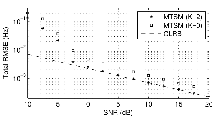
Figure 3: Frequency total root-mean square error for a 3-D signal containing 3 modes with identical modes in two dimensions and close modes in the first dimension (Signal #4 in Table III). $N(0)=20,\eta_{\nu}=21,\eta_{\beta}=11,(M_{1},M_{2},M_{3})=(10,10,10)$. 100 Monte-Carlo.

V-D Identifiability

Based on the assumptions under which Algorithm 3 is operating, the identifiability condition can be stated as $F<M_{1}$ and $\min\{M_{2},....,M_{R}\}\geq 2$. In [33], the condition is $M_{r}\geq 4,r=1,\ldots,R$, and $F\leq\left\lfloor\frac{M_{1}}{2}\right\rfloor\prod_{r=1}^{R}\left\lceil\frac{M_{r}}{2}\right\rceil$.

We note that, when $M_{r}\geq 4,r=1,\ldots,R$, the number of identifiable modes is slightly smaller than in [33], but the proposed algorithm is able to outperform the conventional methods in terms of computational complexity and accuracy. In addition, another advantage of the proposed algorithm is clear when the number of samples in one or more dimensions is less than 4 (i.e. $M_{r}<4$), where identifiability in [33] is not satisfied. This latter case (i.e. $\exists r,M_{r}<4$) can be encountered in signal processing applications when the size of one or more diversities (dimensions in our formulation problem) is less than 4.

VI Cramér-Rao Lower Bounds for $R$-D Cisoids in Noise

In this section, we derive the expressions of the CRLB for the parameters of $R$-D damped exponentials in Gaussian white noise. We then give the CRLB in the cases of single damped and undamped $R$-D cisoids. We consider the $R$-D sinusoidal model given in (3). Let

$$\bm{\theta}=[\omega_{1,1}\ldots\omega_{1,R} \quad\omega_{2,1}\ldots\omega_{F,R}\quad\alpha_{1,1}\ldots\alpha_{1,R}$$

$$\quad\alpha_{2,1}\ldots\alpha_{F,R}\quad\lambda_{1}\ldots\lambda_{F}\quad\phi_{1}\ldots\phi_{F}]^{\mathsf{T}}$$

be the unknown parameter vector. The aim here is to derive the CRLB of the parameters in $\bm{\theta}$.

The joint probability density function (pdf) of $\tilde{\mathbf{y}}$ is

$$p(\tilde{\mathbf{y}};\bm{\theta})=\frac{1}{(\sigma^{2}\pi)^{M}}\exp\left\{-\frac{1}{\sigma^{2}}(\tilde{\mathbf{y}}-\bm{\mu}(\bm{\theta}))^{\mathsf{H}}(\tilde{\mathbf{y}}-\bm{\mu}(\bm{\theta}))\right\}$$ (39)

where $\bm{\mu}(\bm{\theta})$ is the noise-free part of $\mathbf{y}$ and

$$\tilde{\mathbf{y}}= [\tilde{y}(1,\ldots,1,1),\ldots,\tilde{y}(1,\ldots,1,M_{R}),$$

$$\tilde{y}(1,\ldots,2,1),\ldots,\tilde{y}(1,\ldots,2,M_{R}),$$

$$\ldots,\tilde{y}(M_{1},\ldots,M_{R})]^{\mathsf{T}}.$$ (40)

The $i$th entry of $\bm{\mu}(\bm{\theta})$ can be written as:

$$\bm{\mu}(\bm{\theta})_{i}=\sum_{f=1}^{F}c_{f}\prod_{r=1}^{R}a_{f,r}^{t_{i,r}},$$ (41)

for $i=1,\ldots,M$, where

$$t_{i,r}=\left\lfloor\frac{i-1}{\prod_{\ell=r+1}^{R}M_{\ell}}\right\rfloor\quad\mod\quad M_{r},$$ (42)

and $\lfloor\cdot\rfloor$ is the floor function. In the following, we derive the expressions of the CRLB in the general case ($F>1$) and then we deduce the result corresponding to a single $R$-D modal signal ($F=1$).

VI-A Derivation of the CRLB

Given the joint pdf in (39), the $(k,l)$ entry of the Fisher information matrix is [34, 35]:

$$[\mathbf{F}(\bm{\theta})]_{kl}=\frac{2}{\sigma^{2}}\mathrm{Re}\left\{\left[\frac{\partial\bm{\mu}(\bm{\theta})}{\partial\theta_{k}}\right]^{\mathsf{H}}\frac{\partial\bm{\mu}(\bm{\theta})}{\partial\theta_{l}}\right\}.$$ (43)

We now express the derivatives $\partial\bm{\mu}(\bm{\theta})_{i}/\partial\theta_{k}$ for $i=1,\ldots,M$ and $k=1,\ldots,2RF+2F$.

• For $k=1,\ldots,RF$, we have

  $$\frac{\partial\bm{\mu}(\bm{\theta})_{i}}{\partial\theta_{k}}=jt_{i,r(k)}c_{f(k)}\prod_{r=1}^{R}a_{f(k),r}^{t_{i,r}}$$ (44)

  with $r(k)=[(k-1)\,\mod\,R]+1$ and $f(k)=\lfloor(k-1)/R\rfloor+1$.

• For $k=RF+1,\ldots,2RF$:

  $$\frac{\partial\bm{\mu}(\bm{\theta})_{i}}{\partial\theta_{k}}=t_{i,r(k)}c_{f(k)}\prod_{r=1}^{R}a_{f(k),r}^{t_{i,r}}$$ (45)

  with $r(k)=[(k-RF-1)\,\mod\,R]+1$ and $f(k)=\lfloor(k-RF-1)/R\rfloor+1$.

• For $k=2RF+1,\ldots,2RF+F$:

  $$\frac{\partial\bm{\mu}(\bm{\theta})_{i}}{\partial\theta_{k}}=e^{j\phi_{f(k)}}\prod_{r=1}^{R}a_{f(k),r}^{t_{i,r}}$$ (46)

  where $f(k)=k-2RF$.

• For $k=2RF+F+1,\ldots,2RF+2F$:

  $$\frac{\partial\bm{\mu}(\bm{\theta})_{i}}{\partial\theta_{k}}=jc_{f(k)}\prod_{r=1}^{R}a_{f(k),r}^{t_{i,r}}$$ (47)

  where $f(k)=k-2RF-F$.

Hence, the $M\times(2RF+2F)$ matrix $\partial\bm{\mu}(\bm{\theta})/\partial\bm{\theta}$ expresses as

$$\frac{\partial\bm{\mu}(\bm{\theta})}{\partial\bm{\theta}} =\underbrace{[j\mathbf{Z}^{\prime}\bm{\Phi}\quad\mathbf{Z}^{\prime}\bm{\Phi}\quad\mathbf{Z}\bm{\phi}\quad j\mathbf{Z}\bm{\phi}]}_{\mathbf{V}}\cdot\underbrace{\textrm{blkdiag}(\bm{\Lambda},\bm{\Lambda},\mathbf{I}_{F},\bm{\lambda})}_{\mathbf{S}}$$ (48)

where

$$\mathbf{Z}^{\prime} =[\mathbf{Z}^{\prime}_{1},\ldots,\mathbf{Z}^{\prime}_{F}]\in\mathbb{C}^{M\times RF},\text{with }\mathbf{Z}^{\prime}_{f}(i,l)=t_{i,l}\prod_{r=1}^{R}a_{f,r}^{t_{i,r}},$$ (49)

$$\bm{\Lambda} =\mathrm{blkdiag}(\lambda_{1}\mathbf{I}_{R},\ldots,\lambda_{F}\mathbf{I}_{R})\in\mathbb{R}^{RF\times RF},$$ (50)

$$\bm{\Phi} =\mathrm{blkdiag}(e^{j\phi_{1}}\mathbf{I}_{R},\ldots,e^{j\phi_{F}}\mathbf{I}_{R})\in\mathbb{C}^{RF\times RF},$$ (51)

$$\mathbf{Z} =[\mathbf{z}_{1},\ldots,\mathbf{z}_{F}]\in\mathbb{C}^{M\times F},\text{with }\mathbf{z}_{f}(i)=\prod_{r=1}^{R}a_{f,r}^{t_{i,r}},$$ (52)

$$\bm{\lambda} =\mathrm{diag}([\lambda_{1},\ldots,\lambda_{F}])\in\mathbb{R}^{F\times F},$$ (53)

$$\bm{\phi} =\mathrm{diag}([e^{j\phi_{1}},\ldots,e^{j\phi_{F}}])\in\mathbb{C}^{F\times F}.$$ (54)

Finally, the inverse of the Fisher information matrix is

$$\mathbf{F}^{-1}(\bm{\theta})=\frac{\sigma^{2}}{2}\mathbf{S}^{-1}\left[\mathrm{Re}\{\mathbf{V}^{\mathsf{H}}\mathbf{V}\}\right]^{-1}\mathbf{S}^{-1}=\frac{\sigma^{2}}{2}\mathbf{S}^{-1}\mathbf{W}\mathbf{S}^{-1}$$ (55)

where $\textrm{Re}\{\cdot\}$ stands for the real part. The CRLB of $\theta_{k}$ is given by $[\mathbf{F}^{-1}(\bm{\theta})]_{kk}$. More explicitly, for $f=1,\ldots,F$ and $r=1,\ldots,R$:

$$\mathrm{CRLB}(\omega_{f,r}) =\frac{2\sigma^{2}\mathbf{W}_{R(f-1)+r,R(f-1)+r}}{\lambda_{f}^{2}}$$ (56)

$$\mathrm{CRLB}(\alpha_{f,r}) =\frac{2\sigma^{2}\mathbf{W}_{RF+R(f-1)+r,RF+R(f-1)+r}}{\lambda_{f}^{2}}$$ (57)

$$\mathrm{CRLB}(\lambda_{f}) =2\sigma^{2}\mathbf{W}_{2RF+f,2RF+f}$$ (58)

$$\mathrm{CRLB}(\phi_{f}) =\frac{2\sigma^{2}\mathbf{W}_{2RF+F+f,2RF+F+f}}{\lambda_{f}^{2}}$$ (59)

Theorem 4

For the general $R$-D exponential process, the CRLB’s for $f=1,\ldots,F$ and $r=1,\ldots,R$ satisfy

$$\mathrm{CRLB}(\omega_{f,r}) =\mathrm{CRLB}(\alpha_{f,r})$$ (60)

$$\mathrm{CRLB}(\lambda_{f}) =\lambda^{2}\mathrm{CRLB}(\phi_{f})$$ (61)

Proof:

It is based on the special block structure of matrix $\mathrm{Re}\{\mathbf{V}^{\mathsf{H}}\mathbf{V}\}$ (see for instance [34]). ∎

VI-B Single Mode Case

In this section, the CRLB’s will be simplified in the case of a single $R$-D modal signal ($F=1$) to obtain more precise details on their parameter dependency. For the sake of simplicity, the subscripts denoting the mode $f=1$ will be omitted. First, assume that $|a_{r}|=\exp(\alpha_{r})<1$. We shall express the products $\mathbf{Z}^{\prime{\mathsf{H}}}\mathbf{Z}^{\prime}$, $\mathbf{Z}^{\mathsf{H}}\mathbf{Z}$ and $\mathbf{Z}^{\prime{\mathsf{H}}}\mathbf{Z}$. After some calculations, we get:

$$[\mathbf{Z}^{\prime{\mathsf{H}}}\mathbf{Z}^{\prime}]_{nk} =\prod_{\begin{subarray}{c}r=1\\ r\neq n,k\end{subarray}}^{R}\left(\frac{1-|a_{r}|^{2M_{r}}}{1-|a_{r}|^{2}}\right)$$

$$\times\begin{cases}\displaystyle\sum_{m=0}^{M_{n}-1}m|a_{n}|^{2m}\displaystyle\sum_{m=0}^{M_{k}-1}m|a_{k}|^{2m},&\text{if }n\neq k\\ \displaystyle\sum_{m=0}^{M_{n}-1}m^{2}|a_{n}|^{2m},&\text{if }n=k\end{cases}$$ (62)

$$\mathbf{Z}^{\mathsf{H}}\mathbf{Z} =\prod_{r=1}^{R}\left(\frac{1-|a_{r}|^{2M_{r}}}{1-|a_{r}|^{2}}\right)$$ (63)

$$[\mathbf{Z}^{\prime{\mathsf{H}}}\mathbf{Z}]_{n} =\prod_{\begin{subarray}{c}r=1\\ r\neq n\end{subarray}}^{R}\left(\frac{1-|a_{r}|^{2M_{r}}}{1-|a_{r}|^{2}}\right)\times\sum_{m=0}^{M_{n}-1}m|a_{n}|^{2m}.$$ (64)

Denoting $M^{(\alpha)}=\prod_{r=1}^{R}(1-|a_{r}|^{2M_{r}})/(1-|a_{r}|^{2})$, $q_{1}(n)=\sum_{m=0}^{M_{n}-1}m|a_{n}|^{2m}/\sum_{m=0}^{M_{n}-1}|a_{n}|^{2m}$ and $q_{2}(n)=\sum_{m=0}^{M_{n}-1}m^{2}|a_{n}|^{2m}/\sum_{m=0}^{M_{n}-1}|a_{n}|^{2m}$, we then obtain:

$$[\mathbf{P}]_{nk} =M^{(\alpha)}\times\begin{cases}q_{1}(n)q_{1}(k),&\text{if }n\neq k\\ q_{2}(n),&\text{if }n=k\end{cases}$$ (65)

$$\mathbf{G} =M^{(\alpha)}$$ (66)

$$[\mathbf{Q}]_{n} =M^{(\alpha)}q_{1}(n),$$ (67)

and

$$\mathrm{Re}\{\mathbf{V}^{\mathsf{H}}\mathbf{V}\}=\begin{bmatrix}\mathbf{P}&0&0&\mathbf{Q}\\ 0&\mathbf{P}&\mathbf{Q}&0\\ 0&\mathbf{Q}^{\mathsf{T}}&\mathbf{G}&0\\ \mathbf{Q}^{\mathsf{T}}&0&0&\mathbf{G}\end{bmatrix}.$$ (68)

The inversion of $\mathrm{Re}\{\mathbf{V}^{\mathsf{H}}\mathbf{V}\}$ yields the following expressions of the CRLB’s:

$$\mathrm{CRLB}(\omega_{r})=\mathrm{CRLB}(\alpha_{r})=\frac{\sigma^{2}}{2\lambda^{2}M^{(\alpha)}}\\ \quad\times\frac{(1-|a_{r}|^{2})^{2}(1-|a_{r}|^{2M_{r}})^{2}}{[-M_{r}^{2}|a_{r}|^{2M_{r}}(1-|a_{r}|^{2})^{2}+|a_{r}|^{2}(1-|a_{r}|^{2M_{r}})^{2}]},$$ (69)

$$\frac{\mathrm{CRLB}(\lambda)}{\lambda^{2}}=\mathrm{CRLB}(\phi)=\frac{\sigma^{2}}{2\lambda^{2}M^{(\alpha)}}\\ \quad\times\left(1+\sum_{r=1}^{R}\frac{q_{1}^{2}(r)}{q_{2}(r)-q_{1}^{2}(r)}\right).$$ (70)

Finally, for a single $R$-D purely harmonic signal ($\alpha_{r}=0,\forall r$), we have $M^{(\alpha)}=\prod_{r=1}^{R}M_{r}=M$ and taking the limit of the CRLB’s when $\alpha_{r}\to 0$ leads to:

$$\lim_{\alpha_{r}\to 0}\mathrm{CRLB}(\omega_{r}) =\frac{6\sigma^{2}}{\lambda^{2}M(M_{r}^{2}-1)}$$ (71)

$$\lim_{\alpha_{r}\to 0}\frac{\mathrm{CRLB}(\lambda)}{\lambda^{2}} =\frac{\sigma^{2}}{2\lambda^{2}M}\left(1+3\sum_{r=1}^{R}\frac{M_{r}-1}{M_{r}+1}\right).$$ (72)

Hence, for the undamped case, our result in (71) is consistent with [11].

VII Simulation Results

Numerical simulations have been carried out to assess the performances of the proposed method for 2-D and 3-D modal signals in the presence of white Gaussian noise. The performances are measured by the total root-mean square error (RMSE) on estimated parameters and the computational time. The total RMSE is defined as $\mathrm{RMSE}_{\mathrm{total}}=\sqrt{\frac{1}{RF}\mathbb{E}_{p}\left\{\sum_{r=1}^{R}\sum_{f=1}^{F}(\xi_{f,r}-\hat{\xi}_{f,r})^{2}\right\}}$ where $\hat{\xi}_{f,r}$ is an estimate of $\xi_{f,r}$, and $\mathbb{E}_{p}$ is the average on $p$ Monte-Carlo trials. In our simulations, $\xi_{f,r}$ can be either a frequency or a damping factor.

VII-A RMSE for 2-D and 3-D Signals

Experiment 1

to show the interest of the multigrid scheme, this experiment presents the results obtained on Signal #1 with different multigrid levels and different initial grids. Signal #1 is a single tone 2-D modal signal of size $10\times 10$ whose parameters are presented in Table I. The number of multigrid levels is fixed to $L=2$, i.e., $\ell=0,1,2$. Then the results are presented as a function of the number of atoms in the initial dictionaries $N(0)$ and the number of atoms $\eta_{\nu}$ or $\eta_{\alpha}$ added at each level $\ell$. The results we obtain for the first step, i.e., for the harmonic estimation, are presented in Figure 4. We can observe that the frequency RMSE obtained with the $R$-D sparse algorithm can reach the CRLB using a uniform initial harmonic dictionary of 10 atoms and $\color[rgb]{0,0,0}\eta_{\nu}\color[rgb]{0,0,0}=31$ (Figure 4.a). Figure 4.b shows that the frequency RMSE is improved at low SNR if the initial dictionary contains 20 atoms, and reaches the optimal estimates with $\color[rgb]{0,0,0}\eta_{\nu}\color[rgb]{0,0,0}=21$. Figure 5 shows the damping factor RMSE obtained by $R$-D sparse algorithm using different settings of the initial damping factor dictionary and $\eta_{\alpha}$. We can observe that the damping factor RMSE depends on the number of atoms in the dictionary, the more atoms the better. At low SNR, the RMSE also depends $\beta_{\min}$. Therefore, it is better to choose $\beta_{\min}$ with small absolute value if we have a prior knowledge of the interval of damping factors in the signal. In general, the estimation error is of order $\frac{1}{N(0)\eta^{2}}$. For instance, in the frequency step estimation, we recommend to chose $N(0)$ to be greater than or equal to $\frac{3}{2}M_{r}$ if we want a good accuracy at lower SNR levels. Otherwise, we can set $N(0)=M_{r}$. Once $N(0)$ is set, $\eta$ can be chosen with respect to the desired accuracy. Let $\varepsilon$ be the desired estimation error, then $\varepsilon=\frac{1}{N(0)\eta^{2}}$ and we can set $\eta=\frac{1}{\sqrt{\varepsilon N(0)}}$.

TABLE I: 2-D parameters of Signal #1

$f$	$\nu_{f,1}$	$\alpha_{f,1}$	$\nu_{f,2}$	$\alpha_{f,2}$	$c_{f}$
1	$0.22$	$-0.011$	$0.34$	$-0.015$	1

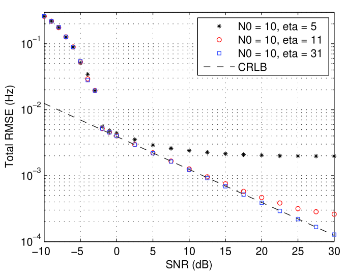
(a) $N(0)=10$

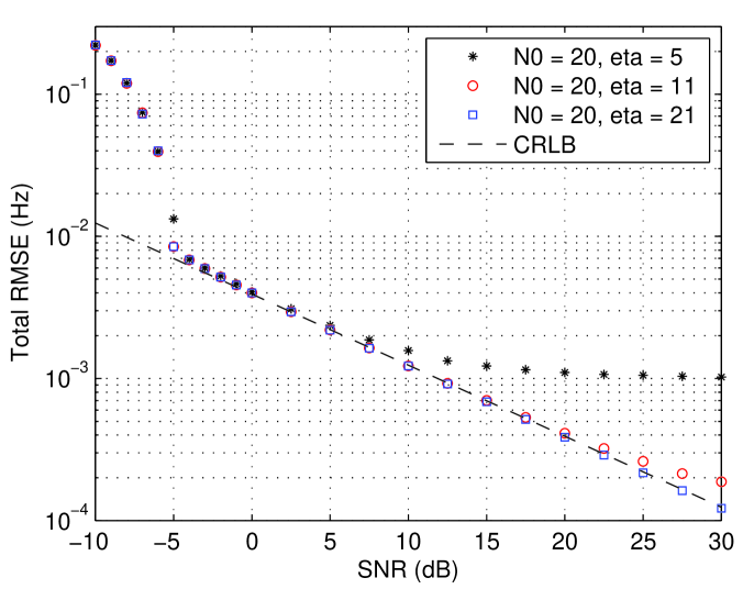
(b) $N(0)=20$

Figure 4: Frequency RMSE using $R$-D sparse algorithm with different $\eta_{\nu}$. 2-D signal containing a single tone (Signal #1). $(M_{1},M_{2})=(10,10).$ 1000 Monte-Carlo trials. (a) The initial harmonic dictionary contains $N(0)=10$ atoms, (b) $N(0)=20$ atoms.

\psfrag{N0 = 04, eta= 05, betaMin = -2}[cc][cc]{\tiny$N(0)=04,\eta_{\alpha}=05,\beta_{\min}=-2$ }\psfrag{N0 = 20, eta= 21, betaMin = -2}[cc][cc]{\tiny$N(0)=20,\eta_{\alpha}=21,\beta_{\min}=-2$ }\psfrag{N0 = 10, eta= 11, betaMin = -0.05}[cc][cc]{\tiny$N(0)=10,\eta_{\alpha}=11,\beta_{\min}=-0.05$ }\psfrag{CRLB}[cc][cc]{\tiny CRLB }\includegraphics[width=352.97124pt]{fig_eta_beta}

Figure 5: Damping factor RMSE using $R$-D sparse algorithm with different $\eta_{\alpha}$, $\beta_{\min}$ and $N(0)$. 2-D signal containing a single tone (Signal #1). $(M_{1},M_{2})=(10,10).$ 1000 Monte-Carlo trials.

In the rest of this section, the proposed algorithms are compared with 2-D ESPRIT [6], Tensor-ESPRIT [10], PUMA [12] and TPUMA [11]. If the $R$-D signal contains one tone then Algorithm 2 (STSM) is used, otherwise Algorithm 3 (MTSM) is used. Thus, to facilitate notation, both proposed algorithms, Algorithm 2 and Algorithm 3, will be called $R$-D sparse. For the proposed method, the initial grid used to build the harmonic dictionary is the same for all dimensions; it contains $50$ frequency points uniformly distributed over the interval $[0,1)$ and 10 damping factors $\beta\in[-0.05,0]$. To simulate a random dictionary, at each run, the frequency grid is perturbed by a small random quantity. As a consequence of experiment 1, we use the following settings $(L,\eta_{\mu},\eta_{\beta})=(2,21,11)$. The number of iterations in Algorithm 3 is set to $K=2$ because no improvement was observed for $K>2$.

Since the proposed method is applied directly on data without using spatial smoothing, i.e., it does not require the construction of a large matrix or an augmented order tensor, then a relevant comparison will be with algorithms that do not use spatial smoothing. Thereby, in the next experiments, the proposed algorithm is compared to PUMA [12] and TPUMA [11], which are algorithms that do not require spatial smoothing. We also report comparisons with 2-D ESPRIT [6] and Tensor-ESPRIT [10], which need spatial smoothing.

VII-A1 Single tone $R$-D modal signal

Experiment 2

This experiment tends to show the efficiency of the proposed algorithm in estimating parameters of single tone $R$-D modal signals. We simulate a 2-D signal of size $10\times 10$ (Signal #1) whose parameters are presented in Table I. Our $R$-D sparse algorithm is compared to 2-D ESPRIT [6] and PUMA [12]. For each level of noise, 1000 Monte-Carlo trials are performed. Figure 6 shows the obtained results. We can observe that: i) the proposed algorithm and PUMA reach the CRLB and outperform 2-D ESPRIT, ii) $R$-D sparse outperform PUMA in SNR less than 3 dB.

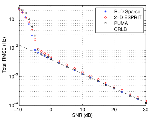
Figure 6: Frequency total root-mean square error for a 2-D signal containing a single tone (Signal #1). $(M_{1},M_{2})=(10,10).$ 1000 Monte-Carlo trials.

VII-A2 Multiple tones R-D modal signals

Several configurations are studied in the case of multiple tones to compare the proposed algorithm with Tensor-ESPRIT [10] and TPUMA [11]. These configurations (Experiments 3, 4, 5) are summarized in Table II, in which the number of modes and the distance between frequencies in different dimensions are varied. $\Delta_{\mathrm{Fr}}$ denotes the Rayleigh frequency resolution limit, which has the same value in all dimensions because $M_{1}=M_{2}=M_{3}$. In Experiment 6 we examine the case when the size of only one dimension is larger than 4, i.e., the identifiability condition of [33] is not satisfied. The parameters of the used signals are given in Table III.

TABLE II: Different configurations for experiments 3 through 5

	$F$	Dimension 1	Dimension 2	Dimension 3
Exp. 3	2	$\Delta\nu>\Delta_{\mathrm{Fr}}$	$\Delta\nu>\Delta_{\mathrm{Fr}}$	$\Delta\nu>\Delta_{\mathrm{Fr}}$
Exp. 4	3	$\Delta\nu\geq\Delta_{\mathrm{Fr}}$	$\exists$ identical modes	$\exists$ identical modes
Exp. 5	3	$\Delta\nu<\Delta_{\mathrm{Fr}}$	$\exists$ identical modes	$\exists$ identical modes

TABLE III: 3-D parameters of Signal #2 through #5

Signal	$\nu_{f,1}$	$\alpha_{f,1}$	$\nu_{f,2}$	$\alpha_{f,2}$	$\nu_{f,3}$	$\alpha_{f,3}$	$c_{f}$
#2	$0.40$	$-0.01$	$0.1$	$-0.01$	$0.1$	$-0.01$	1
	$0.20$	$-0.01$	$0.3$	$-0.15$	$0.25$	$-0.01$	1
#3	$0.30$	$-0.01$	$0.31$	$-0.01$	$0.22$	$-0.01$	1
	$0.10$	$-0.01$	$0.45$	$-0.015$	$0.11$	$-0.01$	1
	$0.20$	$-0.01$	$0.31$	$-0.01$	$0.11$	$-0.01$	1
#4	$0.28$	$-0.01$	$0.31$	$-0.01$	$0.22$	$-0.01$	1
	$0.12$	$-0.01$	$0.45$	$-0.015$	$0.11$	$-0.01$	1
	$0.20$	$-0.01$	$0.31$	$-0.01$	$0.11$	$-0.01$	1
#5	$0.30$	$-0.01$	$0.1$	$-0.01$	$0.1$	$-0.01$	1
	$0.13$	$-0.01$	$0.45$	$-0.015$	$0.4$	$-0.01$	1
	$0.20$	$-0.01$	$0.31$	$-0.01$	$0.1$	$-0.01$	1
	$0.42$	$-0.012$	$0.22$	$-0.01$	$0.32$	$-0.01$	1

Experiment 3

In this experiment, we simulate a 3-D signal (Signal #2) of size $8\times 8\times 8$ and containing two modes whose frequencies in each dimension are well separated. Parameters of the signal are given in Table III. Figure 7 shows the obtained results. Here, the proposed method performs as TPUMA. Tensor-ESPRIT yields slightly worse RMSE.

Experiment 4

3-D signal of size $10\times 10\times 10$ containing three 3-D modes (Signal #3). Note that there exists identical modes in two dimensions and frequencies in the first dimension are separated by $1/M_{1}$. Figure 8 shows the results. In this configuration, TPUMA and Tensor-ESPRIT give similar results and the proposed method performs better for all SNR levels.

Experiment 5

3-D signal of size $10\times 10\times 10$ containing three 3-D modes (Signal #4). Note that there exists identical modes in two dimensions and frequencies in the first dimension are separated by less than $1/M_{1}$. The results are shown on Figure 9. Here again the proposed $R$-D sparse approach performs better than TPUMA and Tensor-ESPRIT. Observe also that Tensor-ESPRIT outperforms TPUMA in this configuration (close frequencies and identical modes in dimensions 2-3).

Experiment 6

Results on Signal #5 of size $10\times 3\times 3$ containing 4 modes are given in Figure 10. We observe that the proposed method outperforms TPUMA algorithm mainly in low SNR levels.

VII-B Numerical Complexity

It is known that in the case of 1-D signals of size $M$, OMP costs $\mathrm{O}(NFM)$ in terms of multiplications [36]; $F$ is the sparsity (number of components) and $N$ is the number of atoms in the dictionary. For a $M$-measurements $R$-D signal, the complexity of the STSM algorithm over a set of $L$ multigrid levels is $\mathrm{O}(MNLR)$, assuming that the number of dictionary atoms is maintained constant (equal to $N$) over all levels. Regarding the approach proposed in Algorithm 3, the main operations are the call of STSM and the update of $\widehat{c_{f}{\mathbf{a}}_{f,1}}=\bar{\mathbf{Y}}_{{f}_{(1)}}^{(i)}\left((\hat{\mathbf{a}}_{f,R}\boxtimes\cdots\boxtimes\hat{\mathbf{a}}_{f,2})^{\mathsf{T}}\right)^{\dagger}$ which has a complexity of $\mathrm{O}(M)$ since $\left((\hat{\mathbf{a}}_{f,R}\boxtimes\cdots\boxtimes\hat{\mathbf{a}}_{f,2})^{\mathsf{T}}\right)^{\dagger}$ is a row of length $\prod_{r=2}^{R}M_{r}$ and $\bar{\mathbf{Y}}_{{f}_{(1)}}^{(i)}$ is a matrix of size $M_{1}\times\prod_{r=2}^{R}M_{r}$. Therefore, the whole complexity of the proposed algorithm is $\mathrm{O}\left((NL(F(R-1)K+1)+FK)M\right)$, which is linear in the number of measurements $M$. The complexity of the Tensor-ESPRIT algorithm with spatial smoothing is mainly related to that of the SVD which is at least $\mathrm{O}(k_{t}F(R+1)PM)$ where $k_{t}$ is a constant depending on the implementation of the SVD algorithm. Here $P=\prod_{r=1}^{R}P_{r}$ where $\{P_{r}\}_{r=1}^{R}$ are design parameters used to get smoothed measurements (see [10]). The accuracy of the estimates provided by ESPRIT depends on these parameters. Since the optimal value for $P_{r}$ is a fraction of $M_{r}$ (e.g. [37, 38, 39]), the complexity of the SVD step is, in fact, $\mathrm{O}(M^{2})$. The complexities of PUMA and TPUMA algorithms are $\mathrm{O}(M^{3})$ and $\mathrm{O}(k_{t}M(R+F-1))+\sum_{r=1}^{R}\mathrm{O}(K(F+1)M_{r}^{3})$, respectively. Compared to PUMA and TPUMA, the proposed algorithm has an attractive computational complexity for large size signals. Figure 11 shows the CPU time results of the proposed, Tensor-ESPRIT and TPUMA algorithms versus $M_{1}$ for a $3$-D damped signal containing two modes with $M_{2}=M_{3}=4$. We observe that the proposed method has low computational complexity compared to TPUMA and Tensor-ESPRIT when $M_{1}$ is large.

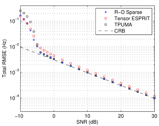
Figure 7: Frequency total root-mean square error for a 3-D signal containing two 3-D modes (Signal #2). $(M_{1},M_{2},M_{3})=(8,8,8).$ 1000 Monte-Carlo.

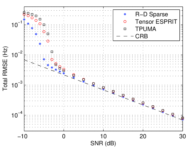
Figure 8: Frequency total root-mean square error for a 3-D signal containing 3 modes with identical modes in two dimensions (Signal #3). $(M_{1},M_{2},M_{3})=(10,10,10).$ 200 Monte-Carlo.

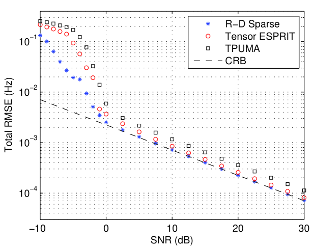
Figure 9: Frequency total root-mean square error for a 3-D signal containing 3 modes with identical modes in two dimensions (Signal #4), same as Signal #4 with close modes in the first dimension (0.28,0.12,0.2). $(M_{1},M_{2},M_{3})=(10,10,10).$ 200 Monte-Carlo.

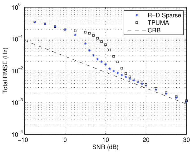
Figure 10: Frequency total root-mean square error for a 3-D signal containing 4 modes with $(M_{1},M_{2},M_{3})=(10,3,3)$ (Signal #5). 200 Monte-Carlo.

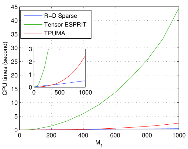
Figure 11: Average CPU time for a single run under $M_{2}=M_{3}=4$ and $F=2$.

VIII Conclusion

We presented an efficient sparse estimation approach for the analysis of multidimensional ($R$-D) damped or undamped modal signals. The idea consists in exploiting the simultaneous sparse approximation principle to separate this joint estimation problem into $R$ multiple measurements problems. To be able to handle large size signals and yield accurate estimates, a multigrid dictionary refinement scheme is associated with the simultaneous orthogonal matching pursuit (SOMP) algorithm. We gave the convergence proof of the the refinement procedure in the single tone case. Then, for the general multiple tones $R$-D case, the signal tensor model is decomposed in order to handle each tone separately in an iterative scheme so that the pairing of the $R$-D parameters is automatically achieved. Also, the CRLB of the $R$-D modal signal parameters were derived. The tests performed on simulated signals showed that the proposed algorithm attains the CRLB and outperforms state-of-the-art subspace algorithms. We also have shown that the complexity of the algorithm is linear with respect to the number of measurements, which allows the processing of large size signals. Finally, it is worth mentioning that this approach can be straightforwardly applied to other multidimensional array processing problems.

Appendix A SOMP Algorithm

In this appendix we report the SOMP method (Algorithm 4) [23]. In this description, $\mathbf{j}_{m_{2}}$ denotes the $m_{2}$^th vector of the canonical basis in $\mathbb{C}^{M_{2}}$.

input : A matrix $\mathbf{Y}\in\mathbb{C}^{M_{1}\times M_{2}}$, a matrix $\mathbf{Q}\in\mathbb{C}^{M_{1}\times N}$ (with normalized columns)

output : An index set $\Omega$ of activated atoms. A matrix of sparse vectors $\mathbf{X}\in\mathbb{C}^{N\times M_{2}}$

initialization: $k=0,\Omega_{0}=\varnothing,\mathbf{X}=\mathbf{0}$, $\mathbf{R}_{0}=\mathbf{Y}$ while halting criterion false do

       $k=k+1$

       $n_{k}\in{\rm arg\ max}_{n}{\sum_{m_{2}=1}^{M_{2}}|\langle\mathbf{R}_{k-1}\mathbf{j}_{m_{2}},\mathbf{q}_{n}\rangle|}$      $\Omega_{k}=\Omega_{k-1}\cup\{n_{k}\}$

       $\mathbf{X}_{k}=(\mathbf{Q}_{\Omega_{k}}^{H}\mathbf{Q}_{\Omega_{k}})^{-1}\mathbf{Q}_{\Omega_{k}}^{H}\mathbf{Y}$     

       $\mathbf{R}_{k}=\mathbf{Y}-\mathbf{Q}_{\Omega_{k}}\mathbf{X}_{k}$

      

end while

return $\Omega=\Omega_{k},\mathbf{X}=\mathbf{X}_{k}$

Algorithm 4 SOMP

Appendix B Proof of Theorem 3

We begin the proof by introducing the following lemma.

Lemma 1

Consider $\widetilde{\bm{\mathcal{Y}}}=\bm{\mathcal{Y}}+\Delta{\bm{\mathcal{Y}}}$, where $\widetilde{\bm{\mathcal{Y}}}$ is the perturbed version of the data tensor $\bm{\mathcal{Y}}$ and $\Delta{\bm{\mathcal{Y}}}$ is the perturbation. Assuming that $\Delta\bm{\mathcal{Y}}$ is sufficiently small such that the ordering of the $F$ singular values in $\bm{\Sigma}$ in (30) is the same as the ordering of the corresponding singular values when $\Delta\bm{\mathcal{Y}}=0$. Then the perturbation $\Delta\bm{\mathcal{Y}}_{f}$ contains a linear combination of all $\bm{\mathcal{Y}}_{f},f=1,\ldots,F$:

$$\Delta\bm{\mathcal{Y}}_{f}=\bm{\mathcal{D}}_{f}+\sum_{i=1}^{F}v_{f,i}\bm{\mathcal{Y}}_{i}$$

where $\mathbf{v}_{f}^{\mathsf{T}}=[v_{f,1},\ldots,v_{f,F}]=\Delta\mathbf{A}_{1}^{\dagger}(f,:)\mathbf{A}_{1}$ and $\bm{\mathcal{D}}_{f}=\Delta\bm{\mathcal{Y}}\mathop{\bullet}\limits_{1}\mathbf{a}_{f,1}\mathbf{A}_{1}^{\dagger}(f,:)+\bm{\mathcal{Y}}_{s,f}\mathop{\bullet}\limits_{1}\Delta\mathbf{a}_{f,1}$.

Proof:

From (33) $\color[rgb]{0,0,0}\bm{\mathcal{S}}\color[rgb]{0,0,0}=\bm{\mathcal{Y}}\mathop{\bullet}\limits_{1}\mathbf{A}_{1}^{\dagger}$, we differentiate and obtain

$$\color[rgb]{0,0,0}\Delta\bm{\mathcal{S}}\color[rgb]{0,0,0} =\Delta\bm{\mathcal{Y}}\mathop{\bullet}\limits_{1}\mathbf{A}_{1}^{\dagger}+\bm{\mathcal{Y}}\mathop{\bullet}\limits_{1}\Delta\mathbf{A}_{1}^{\dagger}$$

Then,

$$\color[rgb]{0,0,0}\Delta\bm{\mathcal{S}}_{f}\color[rgb]{0,0,0} =\Delta\bm{\mathcal{Y}}\mathop{\bullet}\limits_{1}\mathbf{A}_{1}^{\dagger}(f,:)+\color[rgb]{0,0,0}\bm{\mathcal{S}}\color[rgb]{0,0,0}\mathop{\bullet}\limits_{1}\underbrace{\Delta\mathbf{A}_{1}^{\dagger}(f,:)\mathbf{A}_{1}}_{\mathbf{v}^{\mathsf{T}}}$$

$$=\Delta\bm{\mathcal{Y}}\mathop{\bullet}\limits_{1}\mathbf{A}_{1}^{\dagger}(f,:)+\color[rgb]{0,0,0}\bm{\mathcal{S}}\color[rgb]{0,0,0}\mathop{\bullet}\limits_{1}\mathbf{v}^{\mathsf{T}}$$

$$=\Delta\bm{\mathcal{Y}}\mathop{\bullet}\limits_{1}\mathbf{A}_{1}^{\dagger}(f,:)+\sum_{p=1}^{F}v_{f,p}\color[rgb]{0,0,0}\bm{\mathcal{S}}_{p}$$

$\bm{\mathcal{Y}}_{f}$ is estimated using $\bm{\mathcal{Y}}_{f}=\color[rgb]{0,0,0}\bm{\mathcal{S}}_{f}\color[rgb]{0,0,0}\mathop{\bullet}\limits_{1}\mathbf{a}_{f,1}$, we differentiate and obtain

$$\Delta\bm{\mathcal{Y}}_{f} =\color[rgb]{0,0,0}\Delta\bm{\mathcal{S}}_{f}\color[rgb]{0,0,0}\mathop{\bullet}\limits_{1}\mathbf{a}_{f,1}+\color[rgb]{0,0,0}\bm{\mathcal{S}}_{f}\color[rgb]{0,0,0}\mathop{\bullet}\limits_{1}\Delta\mathbf{a}_{f,1}$$

$$=\sum_{p=1}^{F}v_{f,p}\bm{\mathcal{Y}}_{p}+\color[rgb]{0,0,0}\bm{\mathcal{S}}_{f}\color[rgb]{0,0,0}\mathop{\bullet}\limits_{1}\Delta\mathbf{a}_{f,1}+\Delta\bm{\mathcal{Y}}\mathop{\bullet}\limits_{1}\mathbf{a}_{f,1}\mathbf{A}_{1}^{\dagger}(f,:)$$

$\blacksquare$ ∎

Using the previous lemma

$$\bar{\bm{\mathcal{Y}}}_{f}^{(0)} =\color[rgb]{0,0,0}\bm{\mathcal{S}}_{f}\color[rgb]{0,0,0}\mathop{\bullet}\limits_{1}(\mathbf{a}_{f,1}+v_{f,f}\mathbf{a}_{f,1}+\Delta\mathbf{a}_{f})+$$

$$\quad\quad\sum_{p=1,p\neq f}^{F}v_{f,p}\bm{\mathcal{Y}}_{p}+\Delta\bm{\mathcal{Y}}\mathop{\bullet}\limits_{1}\mathbf{a}_{f,1}\mathbf{A}_{1}^{\dagger}(f,:)$$

Therefore, $\mathbf{a}_{f,2},\dots,\mathbf{a}_{f,R},f=1,\ldots,F$ can be estimated using STSM algorithm since

$$\bar{\mathbf{Y}}_{{f}_{(r)}}^{(0)} =c_{f}\mathbf{a}_{f,r}(\mathbf{a}_{f,R}\boxtimes\cdots\boxtimes\mathbf{a}_{f,r+1}\boxtimes\mathbf{a}_{f,r-1}\boxtimes$$

$$\quad\quad\cdots\boxtimes(\mathbf{a}_{f,1}+v_{f,f}\mathbf{a}_{f,1}+\Delta\mathbf{a}_{f,1}))$$

$$\quad\quad+\left(\sum_{p=1,p\neq f}^{F}v_{f,p}\bm{\mathcal{Y}}_{p}+\Delta\bm{\mathcal{Y}}\mathop{\bullet}\limits_{1}\mathbf{a}_{f,1}\mathbf{A}_{1}^{\dagger}(f,:)\right)_{(r)}.$$

Since $\bar{\mathbf{Y}}_{{f}_{(1)}}^{(0)}$ has the following form

$$\bar{\mathbf{Y}}_{{f}_{(1)}}^{(0)} =c_{f}(\mathbf{a}_{f,1}+v_{f,f}\mathbf{a}_{f,1}+\Delta\mathbf{a}_{f,1})(\mathbf{a}_{f,R}\boxtimes\cdots\boxtimes\mathbf{a}_{f,2})$$

$$\quad\quad+\left(\sum_{p=1,p\neq f}^{F}v_{f,p}\bm{\mathcal{Y}}_{p}+\Delta\bm{\mathcal{Y}}\mathop{\bullet}\limits_{1}\mathbf{a}_{f,1}\mathbf{A}_{1}^{\dagger}(f,:)\right)_{(1)},$$

we estimate $c_{f}\mathbf{a}_{f,1}$ by least squares once $\mathbf{a}_{f,2},\dots,\mathbf{a}_{f,R}$ are estimated using STSM

$$\color[rgb]{0,0,0}\widehat{{c}_{f}{\mathbf{a}}_{f,1}}\color[rgb]{0,0,0} =\min_{\mathbf{a}}\|\bar{\bm{\mathcal{Y}}}_{f}^{(0)}-\mathbf{a}\mathop{\otimes}\limits\hat{\mathbf{a}}_{f,2}\mathop{\otimes}\limits\cdots\mathop{\otimes}\limits\hat{\mathbf{a}}_{f,R}\|$$

$$=\bar{\mathbf{Y}}_{{f}_{(1)}}^{(0)}\left((\hat{\mathbf{a}}_{f,R}\boxtimes\cdots\boxtimes\hat{\mathbf{a}}_{f,2})^{\mathsf{T}}\right)^{\dagger}$$

So, we put $\hat{\bm{\mathcal{Y}}}_{f}^{(0)}=\color[rgb]{0,0,0}\widehat{{c}_{f}{\mathbf{a}}_{f,1}}\color[rgb]{0,0,0}\mathop{\otimes}\limits\hat{\mathbf{a}}_{f,2}\mathop{\otimes}\limits\cdots\mathop{\otimes}\limits\hat{\mathbf{a}}_{f,R}$ and $\bm{\mathcal{R}}_{f}=\bar{\bm{\mathcal{Y}}}_{f}^{(0)}-\hat{\bm{\mathcal{Y}}}_{f}^{(0)}.$ Therefore, the procedure to estimate ${\bm{\mathcal{Y}}}_{f}$ at iteration $i=0,\ldots,K$ can be summarized in  (34), (35) and (36). Note that this procedure is optimal because STSM and the least squares are optimal when they are used to estimate $\mathbf{a}_{f,2},\dots,\mathbf{a}_{f,R},f=1,\ldots,F$ and $c_{f}\mathbf{a}_{f,1},f=1,\ldots,F$, respectively.

Now we present the technique for improving the estimation of ${\bm{\mathcal{Y}}}_{f}$. Let $\bm{\mathcal{R}}_{F}^{(0)}=\bm{\mathcal{R}}_{0}^{(1)}=\color[rgb]{0,0,0}\tilde{\bm{\mathcal{Y}}}-\sum_{f=1}^{F}\hat{\bm{\mathcal{Y}}}_{f}^{(0)}$ and

$$\hat{\bm{\mathcal{Y}}}_{f}^{(1)} =\smash{\mathop{{\rm arg\,min}}\limits_{\bm{\mathcal{X}}\in\color[rgb]{0,0,0}\mathcal{H}\color[rgb]{0,0,0}}}\ \|\hat{\bm{\mathcal{Y}}}_{f}^{(0)}+\bm{\mathcal{R}}_{f-1}^{(1)}-\bm{\mathcal{X}}\|$$ (73)

where $\bm{\mathcal{R}}_{f}^{(1)}=\hat{\bm{\mathcal{Y}}}_{f}^{(0)}+\bm{\mathcal{R}}_{f-1}^{(1)}-\hat{\bm{\mathcal{Y}}}_{f}^{(1)},f=1,\ldots,F$, and $\hat{\bm{\mathcal{Y}}}_{f}^{(i)}$ is an improved estimate of ${\bm{\mathcal{Y}}}_{f}$. We follow the same procedure as described in equations (34), (35) and (36) to calculate $\hat{\bm{\mathcal{Y}}}_{f}^{(1)}$.

We can state that there is improvement in the estimation of $\bm{\mathcal{Y}}_{f}$ if

$$\left\|\tilde{\bm{\mathcal{Y}}}-\sum_{f=1}^{F}\hat{\bm{\mathcal{Y}}}_{f}^{(1)}\right\|\leq\left\|\tilde{\bm{\mathcal{Y}}}-\sum_{f=1}^{F}\hat{\bm{\mathcal{Y}}}_{f}^{(0)}\right\|$$ (74)

We have $\|\bm{\mathcal{R}}_{0}^{(1)}\|=\|\bar{\bm{\mathcal{Y}}}_{1}^{(0)}-\hat{\bm{\mathcal{Y}}}_{1}^{(0)}+\sum_{f=2}^{F}\bm{\mathcal{R}}_{f}+\color[rgb]{0,0,0}\bm{\mathcal{V}}\color[rgb]{0,0,0}\|$ where $\bm{\mathcal{V}}=\tilde{\bm{\mathcal{Y}}}-\bar{\bm{\mathcal{Y}}}$ and $\bar{\bm{\mathcal{Y}}}=\sum_{f=1}^{F}\bar{\bm{\mathcal{Y}}}_{f}^{(0)}$. It can be verified that

$$\|\bm{\mathcal{R}}_{f}^{(1)}\|=\left\|\left(\bar{\bm{\mathcal{Y}}}_{f}^{(0)}+\sum_{p=1}^{f-1}(\bar{\bm{\mathcal{Y}}}_{p}^{(0)}-\hat{\bm{\mathcal{Y}}}_{p}^{(1)})+\sum_{p=f+1}^{F}\bm{\mathcal{R}}_{p}+\color[rgb]{0,0,0}\bm{\mathcal{V}}\color[rgb]{0,0,0}\right)-\hat{\bm{\mathcal{Y}}}_{f}^{(1)}\right\|$$

$$\|\bm{\mathcal{R}}_{f-1}^{(1)}\|=\left\|\left(\bar{\bm{\mathcal{Y}}}_{f}^{(0)}+\sum_{p=1}^{f-1}(\bar{\bm{\mathcal{Y}}}_{p}^{(0)}-\hat{\bm{\mathcal{Y}}}_{p}^{(1)})+\sum_{p=f+1}^{F}\bm{\mathcal{R}}_{p}+\color[rgb]{0,0,0}\bm{\mathcal{V}}\color[rgb]{0,0,0}\right)-\hat{\bm{\mathcal{Y}}}_{f}^{(0)}\right\|$$

However, from equation (73), $\hat{\bm{\mathcal{Y}}}_{f}^{(1)}$ is the minimizer with respect to $\bm{\mathcal{X}}\color[rgb]{0,0,0}\in\mathcal{H}\color[rgb]{0,0,0}$ of

$$\left\|\left(\bar{\bm{\mathcal{Y}}}_{f}^{(0)}+\sum_{p=1}^{f-1}(\bar{\bm{\mathcal{Y}}}_{p}^{(0)}-\hat{\bm{\mathcal{Y}}}_{p}^{(1)})+\sum_{p=f+1}^{F}\bm{\mathcal{R}}_{p}\right)-{\bm{\mathcal{X}}}\right\|$$

Therefore, $\|\bm{\mathcal{R}}_{f}^{(1)}\|\leq\|\bm{\mathcal{R}}_{f-1}^{(1)}\|,f=1,\ldots,F$. As consequence, $\|\bm{\mathcal{R}}_{F}^{(1)}\|\leq\|\bm{\mathcal{R}}_{F}^{(0)}\|$, which we are seeking in expression (74). Similarly, we can prove that $\|\bm{\mathcal{R}}_{F}^{(i)}\|\leq\|\bm{\mathcal{R}}_{F}^{(i-1)}\|,i>1,$ using the general forms of $\bm{\mathcal{R}}_{f}^{(i)}$ and $\bm{\mathcal{R}}_{f-1}^{(i)}$

$$\bm{\mathcal{R}}_{f}^{(i)} =\left(\bar{\bm{\mathcal{Y}}}_{f}^{(0)}+\sum_{p=1}^{f-1}(\bar{\bm{\mathcal{Y}}}_{p}^{(0)}-\hat{\bm{\mathcal{Y}}}_{p}^{(i)})+\sum_{p=f+1}^{f-1}(\bar{\bm{\mathcal{Y}}}_{p}^{(0)}-\hat{\bm{\mathcal{Y}}}_{p}^{(i-1)})+\bm{\mathcal{V}}\right)$$

$$\quad\quad-\hat{\bm{\mathcal{Y}}}_{f}^{(i)}$$ (75)

$$\bm{\mathcal{R}}_{f-1}^{(i)} =\left(\bar{\bm{\mathcal{Y}}}_{f}^{(0)}+\sum_{p=1}^{f-1}(\bar{\bm{\mathcal{Y}}}_{p}^{(0)}-\hat{\bm{\mathcal{Y}}}_{p}^{(i)})+\sum_{p=f+1}^{f-1}(\bar{\bm{\mathcal{Y}}}_{p}^{(0)}-\hat{\bm{\mathcal{Y}}}_{p}^{(i-1)})+\bm{\mathcal{V}}\right)$$

$$\quad\quad-\hat{\bm{\mathcal{Y}}}_{f}^{(i-1)}$$ (76)

which we are seeking in (38).

Appendix C Acknowledgment

The authors would like to thank PhD Weize Sun for providing them with the TPUMA algorithm code.

References

- [1] P. Stoica and R. Moses, Introduction to Spectral Analysis. Upper Saddle River, NJ: Prentice Hall, 1997.
- [2] A. B. Gershman and N. D. Sidiropoulos, Space-time processing for MIMO communications. Wiley Online Library, 2005.
- [3] D. Nion and S. Sidiropoulos, “Tensor algebra and multidimensional retrieval in signal processing for MIMO radar,” IEEE Trans. Signal Process., vol. 58, no. 1, pp. 5693–5705, 2010.
- [4] J. Sacchini, W. Steedly, and R. Moses, “Two-dimensional Prony modeling and parameter estimation,” IEEE Trans. Signal Process., vol. 41, no. 11, pp. 3127–3137, 1993.
- [5] Y. Hua, “Estimating two-dimensional frequencies by matrix enhancement and matrix pencil,” IEEE Trans. Signal Process., vol. 40, no. 9, pp. 2267–2280, 1992.
- [6] S. Rouquette and M. Najim, “Estimation of frequencies and damping factors by two-dimensional ESPRIT type methods,” IEEE Trans. Signal Process., vol. 49, no. 1, pp. 237–245, 2001.
- [7] K. Mokios, N. Sidiropoulos, M. Pesavento, and C. Mecklenbrauker, “On 3-D harmonic retrieval for wireless channel sounding,” in Proc. IEEE ICASSP, Montreal, Canada, May 2004, pp. ii89–ii92.
- [8] J. Liu and X. Liu, “An eigenvector-based approach for multidimensional frequency estimation with improved identifiability,” IEEE Trans. Signal Process., vol. 54, no. 12, pp. 4543–4556, December 2006.
- [9] J. Liu, X. Liu, and X. Ma, “Multidimensional frequency estimation with finite snapshots in the presence of identical frequencies,” IEEE Trans. Signal Process., vol. 55, pp. 5179–5194, 2007.
- [10] M. Haardt, F. Roemer, and G. Del Galdo, “Higher-order SVD-based subspace estimation to improve the parameter estimation accuracy in multidimensional harmonic retrieval problems,” IEEE Trans. Signal Process., vol. 56, no. 7, pp. 3198–3213, 2008.
- [11] W. Sun and H. C. So, “Accurate and computationally efficient tensor-based subspace approach for multi-dimensional harmonic retrieval,” IEEE Trans. Signal Process., vol. 60, no. 10, pp. 5077–5088, October 2012.
- [12] H. So, F. Chan, W. Lau, and C. Chan, “An efficient approach for two-dimensional parameter estimation of a single-tone,” IEEE Trans. Signal Process., vol. 58, no. 4, pp. 1999–2009, April 2010.
- [13] L. Huang, Y. Wu, H. So, Y. Zhang, and L. Huang, “Multidimensional sinusoidal frequency estimation using subspace and projection separation approaches,” IEEE Trans. Signal Process., vol. 60, no. 10, pp. 5536–5543, 2012.
- [14] C. Lin and W. Fang, “Efficient multidimensional harmonic retrieval: A hierarchical signal separation framework,” IEEE Signal Process. Lett., vol. 20, no. 5, pp. 427–430, May 2013.
- [15] S. Sahnoun, E.-H. Djermoune, and D. Brie, “Sparse multigrid modal estimation: Initial grid selection,” in Proc. European Signal Process. Conf. (EUSIPCO-2012), 2012, pp. 450–454.
- [16] M. Goodwin and M. Vetterli, “Matching pursuit and atomic signal models based on recursive filter banks,” IEEE Trans. Signal Process., vol. 47, no. 7, pp. 1890–1902, 1999.
- [17] D. Malioutov, M. Cetin, and A. Willsky, “A sparse signal recontruction perspective for source localization with sensor arrays,” IEEE Trans. Signal Process., vol. 53, no. 8, pp. 3010–3022, 2005.
- [18] P. Stoica, P. Babu, and J. Li, “SPICE: A sparse covariance-based estimation method for array processing,” IEEE Trans. Signal Process., vol. 59, no. 2, pp. 629–638, 2011.
- [19] S. Sahnoun, E.-H. Djermoune, C. Soussen, and D. Brie, “Sparse multidimensional modal analysis using a multigrid dictionary refinement,” EURASIP J. Adv. Signal Process., March 2012.
- [20] S. Sahnoun, E.-H. Djermoune, and D. Brie, “Sparse modal estimation of 2-D NMR signals,” in Proc. IEEE ICASSP, Vancouver, Canada, May 2013, pp. 8751–8755.
- [21] J. Sward, S. I. Adalbjornsson, and A. Jakobsson, “High resolution sparse estimation of exponentially decaying signals,” in 2014 IEEE International Conference on Acoustics, Speech and Signal Processing (ICASSP). IEEE, 2014, pp. 7203–7207.
- [22] S. I. Adalbjörnsson, J. Swärd, and A. Jakobsson, “High resolution sparse estimation of exponentially decaying two-dimensional signals,” in 22nd European Signal Processing Conference-EUSIPCO 2014. EURASIP, 2014.
- [23] J. Tropp, A. Gilbert, and M. Strauss, “Algorithms for simultaneous sparse approximation. Part I: Greedy pursuit,” Signal Process., vol. 86, pp. 572–588, 2006.
- [24] R. Boyer, “Deterministic asymptotic cramer–rao bound for the multidimensional harmonic model,” Signal Processing, vol. 88, no. 12, pp. 2869–2877, 2008.
- [25] M. Clark and L. Scharf, “Two-dimensional modal anlysis based on maximum likelihood,” IEEE Trans. Signal Process., vol. 42, no. 6, pp. 1443–1451, 1994.
- [26] P. Comon, “Tensors: a brief introduction,” IEEE Sig. Proc. Magazine, vol. 31, no. 3, May 2014, special issue on BSS. hal-00923279.
- [27] T. Kolda and B. Bader, “Tensor decompositions and applications,” SIAM Review, vol. 51, no. 3, pp. 455–500, 2009.
- [28] A. Rakotomamonjy, “Surveying and comparing simultaneous sparse approximation (or group-Lasso) algorithms,” Signal Process., vol. 91, no. 7, pp. 1505–1526, 2011.
- [29] J. Tropp, “Greed is good: algorithmic results for sparse approximation,” IEEE Trans. Inf. Theory, vol. 50, pp. 2231–2242, Oct 2004.
- [30] J.A.Tropp, “Algorithms for simultaneous sparse approximation. Part II: Convex relaxation,” Signal Process., vol. 86, pp. 589–602, March 2006.
- [31] M. Mishali and Y. Eldar, “Reduce and boost: Recovering arbitrary sets jointly sparse vectors,” IEEE Trans. Signal Process., vol. 56, pp. 4692–4702, Oct 2008.
- [32] K. Lee, Y. Bresler, and M. Junge, “Subspace methods for joint sparse recovery,” IEEE Trans. Inf. Theory, vol. 58, pp. 3613–3641, Jun 2012.
- [33] T. Jiang, N. D. Sidiropoulos, and J. M. Ten Berge, “Almost-sure identifiability of multidimensional harmonic retrieval,” Signal Processing, IEEE Transactions on, vol. 49, no. 9, pp. 1849–1859, 2001.
- [34] Y.-X. Yao and S. Pandit, “Cramér-Rao lower bounds for a damped sinusoidal process,” IEEE Trans. Signal Process., vol. 43, no. 4, pp. 878–885, 1995.
- [35] S. Kay, Fundamentals of statistical signal processing. Estimation theory. Englewood Cliffs, New Jersey: Prentice Hall International Editions, 1993.
- [36] J. Tropp and S. Wright, “Computational methods for sparse solution of linear inverse problems,” Proceedings of the IEEE, vol. 98, no. 6, pp. 948–958, 2010.
- [37] A. Lemma, A.-J. van der Even, and E. Deprettere, “Analysis of joint angle-frequency estimation using ESPRIT,” IEEE Trans. Signal Process., vol. 51, pp. 1264–1283, May 2003.
- [38] E.-H. Djermoune and M. Tomczak, “Perturbation analysis of subspace-based methods in estimating a damped complex exponential,” IEEE Trans. Signal Process., vol. 57, no. 11, pp. 4558–4563, 2009.
- [39] Y. Hua and T. Sarkar, “Matrix pencil method for estimating parameters of exponentially damped/undamped sinusoids in noise,” IEEE Trans. Acoust. Speech Signal Process., vol. 38, pp. 814–824, 1990.