Pulsation-driven mean zonal and meridional flows in rotating massive stars

Abstract

Zonal and meridional axisymmetric flows can deeply impact the rotational and chemical evolution of stars. Therefore, momentum exchanges between waves propagating in stars, differential rotation, and meridional circulation must be carefully evaluated. In this work, we study axisymmetric mean flows in rapidly and initially uniformly rotating massive stars driven by small amplitude non-axisymmetric $\kappa$-driven oscillations. We treat them as perturbations of second-order of the oscillation amplitudes and derive their governing equations as a set of coupled linear ordinary differential equations. This allows us to compute 2-D zonal and meridional mean flows driven by low frequency $g$- and $r$-modes in slowly pulsating B (SPB) stars and $p$-modes in $\beta$ Cephei stars. Oscillation-driven mean flows usually have large amplitudes only in the surface layers. In addition, the kinetic energy of the induced 2-D zonal rotational motions is much larger than that of the meridional motions. In some cases, meridional flows have a complex radial and latitudinal structure. We find pulsation-driven and rotation-driven meridional flows can have similar amplitudes. These results show the importance of taking wave – mean flow interactions into account when studying the evolution of massive stars.

1 introduction

It is well known that differential rotation and related viscous turbulent transport, structural adjustments, and applied torques at stellar surfaces drive large-scale meridional circulation in stellar radiation zones (e.g., Zahn 1992; Rieutord 2006; Decressin et al. 2009; Hypolite & Rieutord 2014). When magnetic fields and internal gravity waves are neglected, the magnitudes of the radial component of such meridional flow ($v_{r}$) scales as (e.g., Kippenhahn et al. 2012)

$$v_{r:\rm MC}\sim\frac{LR^{2}}{GM^{2}}\frac{\Omega^{2}}{2\pi G\bar{\rho}},$$ (1)

where $L$, $M$, $R$, $\bar{\rho}$ and $\Omega$ are the luminosity, mass, radius, mean density and angular velocity of the star respectively. It is anticipated that such meridional circulation in rotating stars mix material and transport angular momentum in their interior during their evolution (e.g., Zahn 1992; Talon et al. 1997; Maeder & Zahn 1998; Meynet & Maeder 2000; Mathis & Zahn 2004).

Stellar non-radial pulsations in rotating stars can also drive such non-oscillatory, large-scale fluid motions, which we may call mean flows. Because of dissipative mechanisms, co-rotation resonances and breaking mechanisms (e.g., Andrews & McIntyre 1978a; Lindzen 1981; Goldreich & Nicholson 1989), pulsations transport angular momentum, which induces mean zonal flows leading to differential rotation. Indeed, angular momentum transport by internal gravity waves takes place in rotating stars, if the wave propagation is accompanied by thermal diffusion/critical layers/non-linear breaking processes that lead to damping and/or excitation of the waves (e.g., Press 1981; Schatzman 1993, 1996; Zahn et al. 1997; Alvan et al. 2013; Rogers et al. 2013). For example, if prograde internal gravity waves propagating in a rotating star damp at a certain place, they will deposit their angular momentum, which accelerates zonal rotational motion of the fluid there. On the other hand, when prograde waves are excited in a place, they extract angular momentum from the flow at this location, leading to deceleration of the rotational fluid motion. The opposite results are obtained for retrograde waves. Therefore, extraction and deposition of angular momentum from rotational fluid motion by waves change the zonal velocity field in the interior of rotating stars. Because of the related modification of angular velocity gradients, of the radial and latitudinal components of the momentum equation, and of the equation of heat, waves modify the general 3-D dynamical balance in stellar radiation zones. As a consequence, they also profoundly affect large-scale meridional flows in the radial and latitudinal directions in these regions (e.g., Bretherton 1969; Andrews & McIntyre 1978a; Holton 1982; Mathis et al. 2013; Belkacem et al. 2015a). In the case of small-amplitude linear pulsations, magnitudes of mean flows are of second-order of the amplitudes and their characteristic timescale is the growth or damping timescales of the waves. Then, these pulsation-driven mean flows will impact material mixing and angular momentum transport processes in rotating stars and will affect pulsations in return.

These processes have been relatively well studied for the case of low-mass stars (e.g., Mathis et al. 2013), but poorly investigated for massive stars. Therefore, it is important to investigate the velocity fields and the magnitudes of both zonal and meridional mean flows driven by stellar pulsations in rotating stars and to investigate their geometrical properties and amplitude in the case of massive stars.

The problem of angular momentum transport and redistribution by internal gravity waves in rotating stars has been investigated by many authors for cool stars. For example, for an explanation of the uniform rotation observationally inferred for the radiative core of the Sun until $0.2R_{\odot}$ thanks to helioseismology (e.g., Schou et al. 1998; García et al. 2007), Schatzman (1993) suggested that angular momentum transport by internal gravity waves generated in the external convective envelope can play an essential role to extract angular momentum [see also Zahn et al. (1997); Talon et al. (2002); Talon & Charbonnel (2005); Rogers et al. (2008); Mathis et al. (2008) in the case where the Coriolis acceleration is taken into account; Kumar et al. (1999); Rogers & MacGregor (2010); Mathis & de Brye (2012) in the magnetized case]. More recently, thanks to new asteroseismic information obtained on the weak differential rotation between the surface and the core of low-mass subgiant and red giant stars (e.g., Beck et al. 2012; Mosser et al. 2012; Deheuvels et al. 2012, 2014), the potential extraction of angular momentum by internal gravity waves and normal mixed gravito-acoustic modes have been studied (Talon & Charbonnel 2008; Fuller et al. 2014; Belkacem et al. 2015a,b).

In the case of massive stars, the transport of angular momentum by internal gravity waves has been less studied (Lee & Saio 1993; Pantillon et al. 2007; Lee et al. 2014). Zahn (1975, 1977) investigated the case of gravity waves tidally excited in massive main-sequence stars by the orbital motion of a companion star in a binary system (see also Goldreich & Nicholson 1989). It allowed him to estimate the timescales of circularization of the orbit and of synchronization of the stellar rotation with the orbital motion. However, the impact of internal gravity waves on large-scale meridional flows in these stars has never been studied.

In this context, one important issue is the case of Be stars. Be stars are rapidly rotating main-sequence late-O, B, and early-A stars that have circumstellar gaseous discs, which are responsible for the generation of emission lines (see Rivinius et al. 2013 for a complete review). Gaseous discs in Be stars are thought to be viscous Keplerian discs (Lee et al. 1991). Although mechanisms for disc formation have not been completely identified yet, rapid rotation and pulsations of these stars must be key ingredients. Moreover, to sustain the discs for several decades, a good amount of angular momentum must be continuously supplied to them. Ando (1983, 1986) employed a wave mean flow interaction theory (e.g., Andrews & McIntyre 1976, 1978a,b; Dunkerton 1980; Grimshaw 1984; Craik 1988; Pedlosky 1982; Bühler 2014) to explain episodic mass loss phenomena observed in Be stars (see also Lee et al. 1991, 2014). As suggested by Lee (2013), if enough angular momentum is supplied to the surface regions of rapidly rotating stars, we can construct a steady system composed of a rotating star and a viscous Keplerian disc around the star. As a mechanism to provide the surface layers with angular momentum, we may invoke the rotation-driven meridional circulation (Meynet & Maeder 1997; Ekström et al. 2008; Granada et al. 2013) and/or internal gravity waves, which may be destabilized by the opacity mechanism or stochastically excited by convective motion in the core (see e.g., Rogers et al. 2013; Lee et al. 2014).

In this paper, we are thus interested in velocity fields of pulsation driven mean zonal and meridional flows in rotating massive stars, and we investigate whether the velocity fields of the mean flows can be favorable to a disc formation around Be stars. Therefore, we calculate pulsation-driven mean flows in the interior of rotating SPB and $\beta$ Cephei stars, in which pulsations are mainly excited by the iron opacity bump ($\kappa$) mechanism. Assuming that the pulsation-driven velocity fields are of second-order of the linear pulsation amplitudes, we derive for the second-order perturbations a set of linear ordinary differential equations, which have inhomogeneous terms generated by non-linear products of the eigenfunctions of the pulsation mode. To derive analytical expressions of these non-linear terms, we introduce and use the so-called Spin Weighted Spherical Harmonics and their complex and tedious derivation is detailed in a complete appendix. The set of linear differential equations we solve is given in §2. In §3, we calculate and discuss the properties of second-order velocity fields driven by unstable $g$- and $r$-modes in SPB stars and $p$-modes in $\beta$ Cephei stars assuming moderate rotation of the stars. In §4, we summarize the results we obtained, and we discuss drawbacks and perspectives of this work.

2 Theoretical formalism for mean flows induced by pulsations

2.1 Dynamical equations

The basic equations governing fluid motions in a star are given by

$$\frac{\partial\mbox{\boldmath$v$}}{\partial t}+\mbox{\boldmath$v$}\cdot\nabla\mbox{\boldmath$v$}=-\frac{1}{\rho}\nabla p-\nabla\Phi,$$ (2)

$$\nabla^{2}\Phi=4\pi G\rho,$$ (3)

$$\frac{\partial\rho}{\partial t}+\nabla\cdot\left(\rho\mbox{\boldmath$v$}\right)=0,$$ (4)

$$\rho T\frac{ds}{dt}=\rho\epsilon-\nabla\cdot\mbox{\boldmath$F$},$$ (5)

$$\mbox{\boldmath$F$}=-\lambda\nabla T\quad{\rm with}\quad\lambda={16\sigma_{\rm SB}T^{3}/3\kappa\rho},$$ (6)

where $v$ is the velocity vector of the fluid, $p$ is the pressure, $\rho$ is the mass density, $T$ is the temperature, $s$ is the specific entropy, $F$ is the energy flux vector, $\Phi$ is the gravitational potential, $\epsilon$ is the nuclear energy generation rate per gram, $\kappa$ is the opacity, $G$ is the gravitational constant, and $\sigma_{\rm SB}$ is the Stefan-Boltzmann constant.

We assume that the star pulsates in small amplitudes around the hydrostatic and radiative equilibrium state. If pulsation amplitudes are sufficiently small, any physical quantity $f\left(\mbox{\boldmath$x$},t\right)$ of the star may be represented by

$$f(\mbox{\boldmath$x$},t)=f^{(0)}(\mbox{\boldmath$x$})+f^{\prime}(\mbox{\boldmath$x$},t)+f^{(2)}(\mbox{\boldmath$x$},t)+\cdots,$$ (7)

where $f^{(0)}$ denotes equilibrium quantities, $f^{\prime}$ Eulerian perturbations of first-order, and $f^{(2)}$ Eulerian perturbations of second-order of the pulsation amplitude. The velocity field $\mbox{\boldmath$v$}\left(\mbox{\boldmath$x$},t\right)$ may also be given by

$$\mbox{\boldmath$v$}(\mbox{\boldmath$x$},t)=\mbox{\boldmath$v$}^{(0)}(\mbox{\boldmath$x$})+\mbox{\boldmath$v$}^{\prime}(\mbox{\boldmath$x$},t)+\mbox{\boldmath$v$}^{(2)}(\mbox{\boldmath$x$},t)+\cdots,$$ (8)

and the equilibrium state is assumed to be that of a uniformly rotating star so that, in spherical polar coordinates $(r,\theta,\phi)$,

$$\mbox{\boldmath$v$}^{(0)}=r\sin\theta\Omega\mbox{\boldmath$e$}_{\phi},$$ (9)

where $\Omega$ is the angular velocity of rotation and assumed to be constant, and $\mbox{\boldmath$e$}_{\phi}$ is the unit vector in the azimuthal direction. In this paper, we ignore rotational deformation of the equilibrium state so that $f^{(0)}$ depends only on the radial distance $r$ from the center of the star. We also employ the Cowling approximation, neglecting the Euler perturbation $\Phi^{\prime}$ of the gravitational potential $\Phi$.

2.2 First-order pulsation quantities

For a given equilibrium state of a star, we solve the linear oscillation equation to obtain wave quantities represented by $f^{\prime}$. For uniformly rotating stars, the oscillation equations, which we solve to obtain normal modes, are found, for example, in Lee & Saio (1987) and Lee & Baraffe (1995). Since separation of variables between the radial $(r)$ and angular $(\theta,\phi)$ coordinates is not possible for perturbations in rotating stars, we use finite series expansion to represent the perturbations in terms of spherical harmonic functions $Y_{l}^{m}(\theta,\phi)$ (e.g., Lee & Saio 1987). For the Lagrangian displacement vector $\xi$, we may write

$$\mbox{\boldmath$\xi$}(\mbox{\boldmath$x$},t)=e^{{\rm i}\sigma t}\mbox{\boldmath$\xi$}(\mbox{\boldmath$x$})=e^{{\rm i}\sigma t}\left(\xi_{r}\mbox{\boldmath$e$}_{r}+\xi_{\theta}\mbox{\boldmath$e$}_{\theta}+\xi_{\phi}\mbox{\boldmath$e$}_{\phi}\right),$$ (10)

where $\mbox{\boldmath$e$}_{r}$, $\mbox{\boldmath$e$}_{\theta}$, and $\mbox{\boldmath$e$}_{\phi}$ are the orthonormal basis vectors in spherical polar coordinates, $\sigma$ denotes the oscillation frequency observed in an inertial frame. For a given azimuthal order $m$, the components of $\mbox{\boldmath$\xi$}(\mbox{\boldmath$x$})$ are given by

$${\xi_{r}}(\mbox{\boldmath$x$})=r\sum_{j=1}^{j_{\rm max}}S_{l_{j}}(r)Y_{l_{j}}^{m}(\theta,\phi),$$ (11)

$${\xi_{\theta}}(\mbox{\boldmath$x$})=r\sum_{j=1}^{j_{\rm max}}\left[H_{l_{j}}(r)\frac{\partial}{\partial\theta}Y_{l_{j}}^{m}(\theta,\phi)+T_{l^{\prime}_{j}}(r)\frac{1}{\sin\theta}\frac{\partial}{\partial\phi}Y_{l^{\prime}_{j}}^{m}(\theta,\phi)\right],$$ (12)

$${\xi_{\phi}}(\mbox{\boldmath$x$})=r\sum_{j=1}^{j_{\rm max}}\left[H_{l_{j}}(r)\frac{1}{\sin\theta}\frac{\partial}{\partial\phi}Y_{l_{j}}^{m}(\theta,\phi)-T_{l^{\prime}_{j}}(r)\frac{\partial}{\partial\theta}Y_{l^{\prime}_{j}}^{m}(\theta,\phi)\right],$$ (13)

and the Eulerian pressure perturbation, $p^{\prime}(\mbox{\boldmath$x$},t)=p^{\prime}(\mbox{\boldmath$x$})e^{{\rm i}\sigma t}$, is given by

$$p^{\prime}\left(\mbox{\boldmath$x$}\right)=\sum_{j=1}^{j_{\rm max}}p^{\prime}_{l_{j}}(r)Y_{l_{j}}^{m}\left(\theta,\phi\right),$$ (14)

where $l_{j}=2(j-1)+|m|$ and $l^{\prime}_{j}=l_{j}+1$ for even modes, and $l_{j}=2j-1+|m|$ and $l^{\prime}_{j}=l_{j}-1$ for odd modes for $j=1~{},2~{},3\cdots,~{}j_{\rm max}$. The angular dependence of $p^{\prime}(\mbox{\boldmath$x$})$ is symmetric (antisymmetric) about the equator for even (odd) modes. In addition, we have

$$\mbox{\boldmath$v$}^{\prime}=\delta\mbox{\boldmath$v$}-\mbox{\boldmath$\xi$}\cdot\nabla\mbox{\boldmath$v$}^{(0)}=\frac{d\mbox{\boldmath$\xi$}}{dt}-\mbox{\boldmath$\xi$}\cdot\nabla\mbox{\boldmath$v$}^{(0)}={\rm i}\omega\mbox{\boldmath$\xi$},$$ (15)

where $\omega=\sigma+m\Omega$ is the oscillation frequency observed in the corotating frame of the star, and $\delta\mbox{\boldmath$v$}$ denotes the Lagrangian perturbation of the velocity vector.

2.3 Pulsation driven mean flows

2.3.1 Expansion of second-order equations

We use a theory of wave-mean flow interaction to discuss axisymmetric flows driven by non-axisymmetric oscillations in rotating stars. We regard the axisymmetric flows as mean flows, which contain both zero^th and second-order contributions in the oscillation amplitude. The zero^th order quantities $f^{(0)}$ are those of equilibrium state and are independent of time $t$. The second-order quantities $f^{(2)}$ carry the time dependence of the mean flow. To derive governing equations for the second-order quantities $f^{(2)}$, we use the zonal averaging defined by

$$\overline{f}=\frac{1}{2\pi}\int_{0}^{2\pi}fd\phi,$$ (16)

and if we assume

$$\overline{f^{\prime}}=0,$$ (17)

we have

$$\overline{f}=\overline{f^{(0)}}+\overline{f^{(2)}}.$$ (18)

Here, we have ignored higher order terms $f^{(k)}$ with $k\geq 3$. Hereafter, we simply write $f^{(0)}$ and $f^{(2)}$ for $\overline{f^{(0)}}$ and $\overline{f^{(2)}}$. Because of the zonal averaging, $f^{(0)}$ and $f^{(2)}$ are independent of $\phi$.

When a non-axisymmetric oscillation mode is excited to attain a small but finite amplitude, non-oscillatory fluid flows may arise as a result of second-order effects of the oscillation. Applying the zonal averaging to the basic equations, we obtain a set of differential equations that govern second-order quantities:

$$\frac{{\partial\mbox{\boldmath$v$}^{\left(2\right)}}}{{\partial t}}+\mbox{\boldmath$v$}^{\left(0\right)}\cdot\nabla\mbox{\boldmath$v$}^{\left(2\right)}+\mbox{\boldmath$v$}^{\left(2\right)}\cdot\nabla\mbox{\boldmath$v$}^{\left(0\right)}+\frac{1}{{\rho^{\left(0\right)}}}\nabla p^{\left(2\right)}+g\frac{{\rho^{\left(2\right)}}}{{\rho^{\left(0\right)}}}\mbox{\boldmath$e$}_{r}=-\overline{\mbox{\boldmath$v$}^{\prime}\cdot\nabla\mbox{\boldmath$v$}^{\prime}}+g\overline{\left({\frac{{\rho^{\prime}}}{{\rho^{\left(0\right)}}}}\right)^{2}}\mbox{\boldmath$e$}_{r}+\frac{1}{{\rho^{\left(0\right)}}}\overline{\frac{{\rho^{\prime}}}{{\rho^{\left(0\right)}}}\nabla p^{\prime}},$$ (19)

$$\frac{\partial\rho^{(2)}}{\partial t}+\nabla\cdot\left(\rho^{(0)}\mbox{\boldmath$v$}^{(2)}\right)=-\overline{\nabla\cdot\left(\rho^{\prime}\mbox{\boldmath$v$}^{\prime}\right)},$$ (20)

$$\mbox{\boldmath$F$}^{(2)}=-\lambda^{(0)}\nabla T^{(2)}-\lambda^{(2)}\nabla T^{(0)}-\overline{\lambda^{\prime}\nabla T^{\prime}},$$ (21)

$$\rho^{(0)}T^{(0)}\left(\frac{\partial s^{(2)}}{\partial t}+\mbox{\boldmath$v$}^{(2)}\cdot\nabla s^{(0)}\right) = -\rho^{(0)}T^{(0)}\overline{\left(\frac{T^{\prime}}{T^{(0)}}+\frac{\rho^{\prime}}{\rho^{(0)}}\right)\left(\frac{\partial s^{\prime}}{\partial t}+\mbox{\boldmath$v$}^{\prime}\cdot\nabla s^{(0)}+\mbox{\boldmath$v$}^{(0)}\cdot\nabla s^{\prime}\right)}-\rho^{(0)}T^{(0)}\overline{\mbox{\boldmath$v$}^{\prime}\cdot\nabla s^{\prime}}$$ (22)

$$+\rho^{(0)}\epsilon^{(2)}+\rho^{(2)}\epsilon^{(0)}-\overline{\nabla\cdot\mbox{\boldmath$F$}^{(2)}}+\overline{\rho^{\prime}\epsilon^{\prime}},$$

where $g=-(\rho^{(0)})^{-1}\partial p^{(0)}/\partial r=GM_{r}/r^{2}$ with $M_{r}=\int_{0}^{r}4\pi r^{\prime 2}\rho^{(0)}dr^{\prime}$. Because of the zonal averaging, we have for non-axisymmetric oscillations

$$\overline{f^{\prime}g^{\prime}}=\frac{1}{2\pi}\int_{0}^{2\pi}\Re\left(f^{\prime}(r,\theta)e^{im\phi}\right)\Re\left(g^{\prime}(r,\theta)e^{im\phi}\right)d\phi=\frac{1}{2}\Re\left(f^{\prime*}g^{\prime}\right)=\frac{1}{2}\Re\left(f^{\prime}g^{\prime*}\right),$$ (23)

where the asterisk (*) indicates complex conjugation.

2.3.2 Solving the system of equations

Since the second-order quantities are assumed axisymmetric, we expand the velocity perturbation $\mbox{\boldmath$v$}^{(2)}$ using spherical harmonic functions $Y_{l}^{0}$ as

$${v_{r}^{(2)}}(\mbox{\boldmath$x$},t)=\sum_{k=1}^{k_{\rm max}}\hat{v}_{S,l_{k}}^{(2)}(r,t)Y_{l_{k}}^{0}(\theta,\phi),$$ (24)

$${v_{\theta}^{(2)}}(\mbox{\boldmath$x$},t)=\sum_{k=1}^{k_{\rm max}}\hat{v}_{H,l_{k}}^{(2)}(r,t)\frac{\partial}{\partial\theta}Y_{l_{k}}^{0}(\theta,\phi),$$ (25)

$${v_{\phi}^{(2)}}(\mbox{\boldmath$x$},t)=-\sum_{k=1}^{k_{\rm max}}\hat{v}_{T,l^{\prime}_{k}}^{(2)}(r,t)\frac{\partial}{\partial\theta}Y_{l^{\prime}_{k}}^{0}(\theta,\phi),$$ (26)

and scalar physical quantities, such as pressure perturbation $p^{(2)}$ for example, as

$$p^{(2)}(\mbox{\boldmath$x$},t)=\sum_{k=1}^{k_{\rm max}}p_{l_{k}}^{(2)}(r,t)Y_{l_{k}}^{0}(\theta,\phi),$$ (27)

where $l_{k}=2(k-1)$ and $l^{\prime}_{k}=l_{k}+1$ for $k=1,~{}2,~{}\cdots,~{}k_{\rm max}$. Note that for both even and odd linear modes the $r$ and $\phi$ components of the right-hand-side of equation (19), for example, are symmetric about the equator of the star and the $\theta$ component is antisymmetric. Since the expansion coefficients of $\mbox{\boldmath$v$}^{(2)}$ contain contributions from products $Y_{l}^{-m}Y_{n}^{m}$, we have to set the expansion length $k_{\rm max}\sim 2\times j_{\rm max}$ for the second-order coefficients. The time dependence is included in the expansion coefficient.

By substituting the expansions (24) to (27) into equations (19) to (22), multiplying by a given spherical harmonic function, and integrating over spherical surface, we derive a finite set of differential equations for the expansion coefficients, which depends on $r$ and $t$. To compute the integrals corresponding to non-linear terms, such as $\int(Y_{l_{k}}^{0})^{*}(\overline{\mbox{\boldmath$v$}^{\prime}\cdot\nabla\mbox{\boldmath$v$}^{\prime}})_{r}\sin\theta d\theta d\phi$, we have to evaluate angular integration of products of three spherical harmonic functions, which can be systematically carried out by introducing spin-weighted spherical harmonic functions ${}_{s}Y_{l}^{m}(\theta,\phi)$, the definition and properties of which are summarized in Appendix A (see also, e.g., Newman & Penrose 1966; Varshalovich et al. 1988). In Appendix B1, we introduce a new set of basis vectors $\mbox{\boldmath$e$}_{r}$, $\mbox{\boldmath$e$}_{q}$ and $\mbox{\boldmath$e$}_{\bar{q}}$, and rewrite the velocity and displacement vectors, and basic equations (19) to (22) on this basis. Then, we derive explicit expressions of non-linear terms by using spin-weighted spherical harmonics (Appendix B2). This allows us to obtain ordinary differential equations for the radial functions of the velocity field and scalar quantities (Appendixes B3 and B4).

Using vector notation for the dependent variables of second-order defined as

$$\mbox{\boldmath$z$}_{1}=\left(\matrix{\hat{v}_{S,{l_{1}}}^{(2)}/r\sigma_{0}\cr\hat{v}_{S,{l_{2}}}^{(2)}/r\sigma_{0}\cr\vdots\cr}\right),\quad\mbox{\boldmath$z$}_{2}=\left(\matrix{p^{(2)}_{l_{1}}/gr\rho^{(0)}\cr p^{(2)}_{l_{2}}/gr\rho^{(0)}\cr\vdots\cr}\right),\quad\mbox{\boldmath$z$}_{3}=\left(\matrix{L^{(2)}_{r,l_{1}}/L^{(0)}_{r}\cr L^{(2)}_{r,l_{2}}/L^{(0)}_{r}\cr\vdots\cr}\right),\quad\mbox{\boldmath$z$}_{4}=\left(\matrix{T^{(2)}_{l_{1}}/T^{(0)}\cr T^{(2)}_{l_{2}}/T^{(0)}\cr\vdots\cr}\right),$$ (28)

$$\mbox{\boldmath$z$}_{h}=\left(\matrix{\sqrt{\Lambda_{l_{1}}}\hat{v}_{H,{l_{1}}}^{(2)}/r\sigma_{0}\cr\sqrt{\Lambda_{l_{2}}}\hat{v}_{H,{l_{2}}}^{(2)}/r\sigma_{0}\cr\vdots\cr}\right),\quad\mbox{\boldmath$z$}_{t}=\left(\matrix{\sqrt{\Lambda_{l^{\prime}_{1}}}\hat{v}_{T,{l^{\prime}_{1}}}^{(2)}/r\sigma_{0}\cr\sqrt{\Lambda_{l^{\prime}_{2}}}\hat{v}_{T,{l^{\prime}_{2}}}^{(2)}/r\sigma_{0}\cr\vdots\cr}\right),\quad\mbox{\boldmath$\rho$}^{(2)}=\left(\matrix{\rho^{(2)}_{l_{1}}\cr\rho^{(2)}_{l_{2}}\cr\vdots\cr}\right),$$ (29)

we rewrite equations (144) to (147) as

$$r\frac{\partial\mbox{\boldmath$z$}_{1}}{\partial r}=\mbox{\boldmath$\sf\Lambda$}_{0}^{1/2}\mbox{\boldmath$z$}_{h}-\left(3+rA-\frac{V}{\Gamma_{1}}\right)\mbox{\boldmath$z$}_{1}-\frac{\partial}{\partial\tau}\frac{\mbox{\boldmath$\rho$}^{(2)}}{\rho^{(0)}}+\frac{\mbox{\boldmath$H$}^{0}}{\sigma_{0}\rho^{(0)}},$$ (30)

$$r\frac{\partial\mbox{\boldmath$z$}_{2}}{\partial r}=-\sqrt{2}\bar{f}c_{1}\mbox{\boldmath$\sf C$}_{A}^{1}\mbox{\boldmath$z$}_{t}-\left(rA-\frac{V}{\Gamma_{1}}+U-1\right)\mbox{\boldmath$z$}_{2}-\frac{\mbox{\boldmath$\rho$}^{(2)}}{\rho^{(0)}}-c_{1}\frac{\partial}{\partial\tau}\mbox{\boldmath$z$}_{1}+\frac{\mbox{\boldmath$G$}_{r}^{0}}{g},$$ (31)

$$r\frac{\partial{\mbox{\boldmath$z$}_{3}}}{\partial r}=-c_{2}\left[\frac{\partial{\mbox{\boldmath$z$}_{4}}}{\partial\tau}-\nabla_{ad}V\frac{\partial\mbox{\boldmath$z$}_{2}}{\partial\tau}+V\left(\nabla_{ad}-\nabla\right)\mbox{\boldmath$z$}_{1}\right]+c_{3}\left[\left(\hat{\epsilon}_{T}-\alpha_{T}\right)\mbox{\boldmath$z$}_{4}+\left(\hat{\epsilon}_{p}+\frac{1}{\chi_{\rho}}\right)\mbox{\boldmath$z$}_{2}\right]-\frac{d\ln L_{r}^{(0)}}{d\ln r}\mbox{\boldmath$z$}_{3}-\frac{\mbox{\boldmath$\sf\Lambda$}_{0}}{V\nabla}\mbox{\boldmath$z$}_{4}+\mbox{\boldmath$I$}^{0},$$ (32)

$$r\frac{\partial\mbox{\boldmath$z$}_{4}}{\partial r}=V\nabla\left(4-\hat{\kappa}_{T}+\alpha_{T}\right)\mbox{\boldmath$z$}_{4}-V\nabla\left(\hat{\kappa}_{p}+\frac{1}{\chi_{\rho}}\right)V\mbox{\boldmath$z$}_{2}-V\nabla\mbox{\boldmath$z$}_{3}-V\nabla\mbox{\boldmath$J$}^{0},$$ (33)

and equations (156) and (157) as

$$-\frac{\partial\mbox{\boldmath$z$}_{h}}{\partial\tau}+\bar{f}\mbox{\boldmath$\sf C$}_{B}^{1}\mbox{\boldmath$z$}_{t}=\mbox{\boldmath$\sf\Lambda$}_{0}^{1/2}\frac{\mbox{\boldmath$z$}_{2}}{c_{1}}+\frac{\left(\mbox{\boldmath$G$}_{q}^{0}-\mbox{\boldmath$G$}_{\bar{q}}^{0}\right)}{\sqrt{2}gc_{1}},$$ (34)

$$-\bar{f}\mbox{\boldmath$\sf C$}_{B}^{0}\mbox{\boldmath$z$}_{h}-\frac{\partial\mbox{\boldmath$z$}_{t}}{\partial\tau}=-\sqrt{2}\bar{f}\mbox{\boldmath$\sf C$}_{C}^{0}\mbox{\boldmath$z$}_{1}+\frac{\left(\mbox{\boldmath$G$}_{q}^{1}+\mbox{\boldmath$G$}_{\bar{q}}^{1}\right)}{\sqrt{2}{\rm i}gc_{1}},$$ (35)

where the inhomogeneous terms $\mbox{\boldmath$H$}^{0}$, $\mbox{\boldmath$I$}^{0}$, $\mbox{\boldmath$J$}^{0}$, $\mbox{\boldmath$G$}_{X}^{0}$, and $\mbox{\boldmath$G$}_{X}^{1}$ with $X\equiv\left\{r,~{}q,~{}{\bar{q}}\right\}$ are vectors whose $k$-th components are respectively given by $H_{l_{k}}^{(2)}$, $I^{(2)}_{l_{k}}$, $J_{l_{k}}^{(2)}$, $G_{X,l_{k}}^{(2)}$, and $G_{X,l^{\prime}_{k}}^{(2)}$, which are defined in Appendix B4, and $\mbox{\boldmath$\sf\Lambda$}_{0}$ and $\mbox{\boldmath$\sf\Lambda$}_{0}^{1/2}$ are diagonal matrices whose $k$-th diagonal components are given by $\Lambda_{l_{k}}=l_{k}\left(l_{k}+1\right)$ and $\sqrt{\Lambda_{l_{k}}}$, respectively. Note that $G_{q,l^{\prime}_{k}}^{(2)}-G_{\bar{q},l^{\prime}_{k}}^{(2)}=0$ and $G_{q,l_{k}}^{(2)}+G_{\bar{q},l_{k}}^{(2)}=0$. The symbols $\mbox{\boldmath$\sf C$}_{A}^{1}$, $\mbox{\boldmath$\sf C$}_{B}^{0}$, $\mbox{\boldmath$\sf C$}_{B}^{1}$, and $\mbox{\boldmath$\sf C$}_{C}^{0}$ denote matrices whose $kj$ components are respectively given by $C_{A}^{l_{k}l^{\prime}_{j}}$, $C_{B}^{l^{\prime}_{k}l_{j}}$, $C_{B}^{l_{k}l^{\prime}_{j}}$, and $C_{C}^{l^{\prime}_{k}l_{j}}$, where $C_{A}^{l_{k}l_{j}}\equiv C_{0(-1)1}^{l_{k}l_{j}1}+C_{01(-1)}^{l_{k}l_{j}1},$ $C_{B}^{l_{k}l_{j}}\equiv C_{1(-1)0}^{l_{k}l_{j}1}+C_{(-1)10}^{l_{k}l_{j}1},$ $C_{C}^{l_{k}l_{j}}\equiv C_{10(-1)}^{l_{k}l_{j}1}+C_{(-1)01}^{l_{k}l_{j}1},$ and the definition of the coefficient $C_{abc}^{ijk}$ is given by (150) in Appendix B3. The physical quantities $V$, $U$, $rA$, $\Gamma_{1}$, $\tau$, $\bar{f}$, and $\sigma_{0}$ in the set of equations (30) to (35) are defined as

$$V=-{d\ln p^{(0)}\over d\ln r},\quad U=\frac{d\ln M_{r}}{d\ln r},\quad rA=\frac{d\ln\rho^{(0)}}{d\ln r}-\frac{1}{\Gamma_{1}}\frac{d\ln p^{(0)}}{d\ln r},\quad\Gamma_{1}=\left(\frac{\partial\ln p}{\partial\ln\rho}\right)_{ad},\quad\tau=\sigma_{0}t,\quad\bar{f}=\sqrt{4\pi\over 3}{\Omega\over\sigma_{0}},$$ (36)

and $\sigma_{0}=\sqrt{GM/R^{3}}$, and the definition of the other physical quantities is given in Appendix B1.

The set of differential equations derived above are partial differential equations with $r$ and $t$ being the independent variables. Since we are interested in mean flows driven by an unstable linear oscillation mode having a complex eigenfrequency $\omega$, the forcing (inhomogeneous) terms in the equations are proportional to $e^{-2\omega_{\rm I}t}$, where $\omega_{\rm I}$ denotes the imaginary part of $\omega$. To make analyses simple, we look for solutions whose time dependence is also given by the factor $e^{-2\omega_{\rm I}t}$, that is, we assume that the partial derivatives $\partial/\partial\tau$ is replaced by the growth or damping rate $\bar{\gamma}=-2\bar{\omega}_{\rm I}$. This simplifying assumption may be justified when we are interested in mean flows driven by self-excited oscillation modes. Since such self-excited oscillation modes must be continually pumped by certain destabilizing mechanisms (e.g., opacity mechanism) even if their amplitudes are saturated by some mechanisms like nonlinear couplings between many different modes, we believe that we have to take account of the effects of this continual pumping of the oscillation modes by introducing the growth rate into the formulation. From equations (34) and (35), we obtain

$$\mbox{\boldmath$z$}_{h}=\mbox{\boldmath$\sf Z$}_{11}\mbox{\boldmath$z$}_{1}+\mbox{\boldmath$\sf Z$}_{12}\mbox{\boldmath$z$}_{2}/c_{1}+\mbox{\boldmath$Z$}_{13},$$ (37)

$$\mbox{\boldmath$z$}_{t}=\mbox{\boldmath$\sf Z$}_{21}\mbox{\boldmath$z$}_{1}+\mbox{\boldmath$\sf Z$}_{22}\mbox{\boldmath$z$}_{2}/c_{1}+\mbox{\boldmath$Z$}_{23},$$ (38)

where

$$\mbox{\boldmath$\sf Z$}_{11}=\sqrt{2}\bar{f}^{2}\mbox{\boldmath$\sf W$}^{-1}_{10}\mbox{\boldmath$\sf C$}_{B}^{1}\mbox{\boldmath$\sf C$}_{C}^{0},\quad\mbox{\boldmath$\sf Z$}_{12}=-\bar{\gamma}\mbox{\boldmath$\sf W$}^{-1}_{10}\mbox{\boldmath$\sf\Lambda$}_{0}^{1/2},\quad\mbox{\boldmath$Z$}_{13}=-\bar{\gamma}\mbox{\boldmath$\sf W$}^{-1}_{10}\frac{\mbox{\boldmath$G$}_{q}^{0}-\mbox{\boldmath$G$}_{\bar{q}}^{0}}{\sqrt{2}gc_{1}}-\bar{f}\mbox{\boldmath$\sf W$}^{-1}_{10}\mbox{\boldmath$\sf C$}_{B}^{1}\frac{\mbox{\boldmath$G$}_{q}^{1}+\mbox{\boldmath$G$}_{\bar{q}}^{1}}{\sqrt{2}{\rm i}gc_{1}},$$ (39)

$$\mbox{\boldmath$\sf Z$}_{21}=\sqrt{2}\bar{\gamma}\bar{f}\mbox{\boldmath$\sf W$}^{-1}_{01}\mbox{\boldmath$\sf C$}_{C}^{0},\quad\mbox{\boldmath$\sf Z$}_{22}=\bar{f}\mbox{\boldmath$\sf W$}^{-1}_{01}\mbox{\boldmath$\sf C$}_{B}^{0}\mbox{\boldmath$\sf\Lambda$}_{0}^{1/2},\quad\mbox{\boldmath$Z$}_{23}=\bar{f}\mbox{\boldmath$\sf W$}^{-1}_{01}\mbox{\boldmath$\sf C$}_{B}^{0}\frac{\mbox{\boldmath$G$}_{q}^{0}-\mbox{\boldmath$G$}_{\bar{q}}^{0}}{\sqrt{2}gc_{1}}-\bar{\gamma}\mbox{\boldmath$\sf W$}^{-1}_{01}\frac{\mbox{\boldmath$G$}_{q}^{1}+\mbox{\boldmath$G$}_{\bar{q}}^{1}}{\sqrt{2}{\rm i}gc_{1}},$$ (40)

$$\mbox{\boldmath$\sf W$}_{10}=\bar{f}^{2}\mbox{\boldmath$\sf C$}_{B}^{1}\mbox{\boldmath$\sf C$}_{B}^{0}+\bar{\gamma}^{2}\mbox{\boldmath$\sf E$},\quad\mbox{\boldmath$\sf W$}_{01}=\bar{f}^{2}\mbox{\boldmath$\sf C$}_{B}^{0}\mbox{\boldmath$\sf C$}_{B}^{1}+\bar{\gamma}^{2}\mbox{\boldmath$\sf E$},$$ (41)

and $\sf E$ is the unit matrix. Substituting equations (37) and (38) into equations (30) to (33), we finally obtain

$$r\frac{\partial\mbox{\boldmath$z$}_{1}}{\partial r}=\left[-\left(3+rA-\frac{V}{\Gamma_{1}}\right)\mbox{\boldmath$\sf E$}+\mbox{\boldmath$\sf\Lambda$}_{0}^{1/2}\mbox{\boldmath$\sf Z$}_{11}\right]\mbox{\boldmath$z$}_{1}-\left(\bar{\gamma}\frac{V}{\chi_{\rho}}\mbox{\boldmath$\sf E$}-\frac{\mbox{\boldmath$\sf\Lambda$}_{0}^{1/2}\mbox{\boldmath$\sf Z$}_{12}}{c_{1}}\right){\mbox{\boldmath$z$}_{2}}+\bar{\gamma}\frac{\chi_{T}}{\chi_{\rho}}\mbox{\boldmath$z$}_{4}-\bar{\gamma}\mbox{\boldmath$R$}^{0}+\mbox{\boldmath$\sf\Lambda$}_{0}^{1/2}\mbox{\boldmath$Z$}_{13}+\frac{\mbox{\boldmath$H$}^{0}}{\sigma_{0}\rho},$$ (42)

$$r\frac{\partial\mbox{\boldmath$z$}_{2}}{\partial r}=-c_{1}\left(\sqrt{2}\bar{f}\mbox{\boldmath$\sf C$}_{A}^{1}\mbox{\boldmath$\sf Z$}_{21}+\bar{\gamma}\mbox{\boldmath$\sf E$}\right)\mbox{\boldmath$z$}_{1}-\left[\left(rA-\frac{V}{\Gamma_{1}}+U-1+\frac{V}{\chi_{\rho}}\right)\mbox{\boldmath$\sf E$}+\sqrt{2}\bar{f}\mbox{\boldmath$\sf C$}_{A}^{1}\mbox{\boldmath$\sf Z$}_{22}\right]\mbox{\boldmath$z$}_{2}+\frac{\chi_{T}}{\chi_{\rho}}\mbox{\boldmath$z$}_{4}-\sqrt{2}\bar{f}c_{1}\mbox{\boldmath$\sf C$}_{A}^{1}\mbox{\boldmath$Z$}_{23}-\mbox{\boldmath$R$}^{0}+\frac{\mbox{\boldmath$G$}_{r}^{0}}{g},$$ (43)

$$r\frac{\partial{\mbox{\boldmath$z$}_{3}}}{\partial r}=-c_{2}\left[\bar{\gamma}\left({\mbox{\boldmath$z$}_{4}}-\nabla_{ad}V{\mbox{\boldmath$z$}_{2}}\right)+V\left(\nabla_{ad}-\nabla\right)\mbox{\boldmath$z$}_{1}\right]+c_{3}\left[\left(\hat{\epsilon}_{T}-\alpha_{T}\right)\mbox{\boldmath$z$}_{4}+\left(\hat{\epsilon}_{p}+\frac{1}{\chi_{\rho}}\right)\mbox{\boldmath$z$}_{2}\right]-\frac{d\ln L_{r}^{(0)}}{d\ln r}\mbox{\boldmath$z$}_{3}-\frac{\mbox{\boldmath$\sf\Lambda$}_{0}}{V\nabla}\mbox{\boldmath$z$}_{4}+\mbox{\boldmath$I$}^{0},$$ (44)

$$r\frac{\partial\mbox{\boldmath$z$}_{4}}{\partial r}=-V\nabla\left(\hat{\kappa}_{p}+\frac{1}{\chi_{\rho}}\right)V\mbox{\boldmath$z$}_{2}-V\nabla\mbox{\boldmath$z$}_{3}+V\nabla\left(4-\hat{\kappa}_{T}+\alpha_{T}\right)\mbox{\boldmath$z$}_{4}-V\nabla\mbox{\boldmath$J$}^{0},$$ (45)

where we have used

$$\frac{\mbox{\boldmath$\rho$}^{(2)}}{\rho^{(0)}}=-\frac{\chi_{T}}{\chi_{\rho}}{\mbox{\boldmath$z$}_{4}}+\frac{V}{\chi_{\rho}}\mbox{\boldmath$z$}_{2}+\mbox{\boldmath$R$}^{0},$$ (46)

and the $k$-th component of the vector $\mbox{\boldmath$R$}^{0}$ is given by

$$R_{k}=\int{}_{0}Y_{k}^{0}Q^{(2)}(\rho)d\Omega,$$ (47)

and the definition of the symbol $Q^{(2)}(\rho)$ is given by (110). The set of differential equations from (42) to (45) is regarded as the mean flow equation solved in this paper. The matrix $\hat{\mbox{\boldmath$\sf W$}}\equiv-\gamma\mbox{\boldmath$\sf\Lambda$}_{0}^{1/2}\mbox{\boldmath$\sf Z$}_{12}$ is a symmetric matrix corresponding to the matrix $\sf W$ discussed, for example, by Lee & Saio (1997) in the traditional approximation. In fact, replacing $\gamma$ by ${\rm i}\omega$ makes $\hat{\mbox{\boldmath$\sf W$}}$ reduce to $\sf W$. We also note that $\sqrt{2}\bar{f}\mbox{\boldmath$\sf C$}_{A}^{1}\mbox{\boldmath$\sf Z$}_{22}=\left(\mbox{\boldmath$\sf\Lambda$}_{0}^{1/2}\mbox{\boldmath$\sf Z$}_{11}\right)^{T}$.

For the boundary conditions applied at the stellar center, we require that the functions $\mbox{\boldmath$z$}_{1}$ and $\mbox{\boldmath$z$}_{2}$ are regular and that $ds/dt=0$, which leads to

$$\bar{\gamma}\left(\frac{T^{(2)}}{T^{(0)}}-\nabla_{ad}V\frac{p^{(2)}}{\rho^{(0)}gr}\right)-\frac{v_{r}^{(2)}}{r\sigma_{0}}V\left(\nabla-\nabla_{ad}\right)=-\frac{\overline{{\rm i}\omega\mbox{\boldmath$\xi$}\cdot\nabla s^{\prime}}}{c_{p}}-\bar{\gamma}\frac{s^{(0)}}{c_{p}}Q^{(2)}(s).$$ (48)

The outer boundary conditions applied at the stellar surface are given by the conditions $dp/dt=0$ and $L_{r}=4\pi r^{2}\sigma_{\rm SB}T^{4}$, from which we derive

$$\bar{\gamma}\frac{p^{(2)}}{\rho^{(0)}gr}-\frac{v_{r}^{(2)}}{r\sigma_{0}}=-\frac{\overline{{\rm i}\bar{\omega}\mbox{\boldmath$\xi$}\cdot\nabla p^{\prime}}}{\rho^{(0)}gr}$$ (49)

and

$$\frac{L_{r}^{(2)}}{L_{r}^{(0)}}-4\frac{T^{(2)}}{T^{(0)}}=-\frac{\overline{\mbox{\boldmath$\xi$}\cdot\nabla L_{r}^{(1)}}}{L_{r}^{(0)}}+4\frac{1}{T^{(0)}}\overline{\left(\mbox{\boldmath$\xi$}\cdot\nabla\delta T^{(1)}+\frac{1}{2}\frac{\partial^{2}T^{(0)}}{\partial r^{2}}\xi_{r}\xi_{r}\right)}+6\overline{\left(\frac{\delta T^{(1)}}{T^{(0)}}\right)^{2}}+\overline{\left(\frac{\xi_{r}}{r}\right)^{2}}+8\overline{\frac{\xi_{r}}{r}\frac{\delta T^{(1)}}{T^{(0)}}},$$ (50)

where

$$\delta T^{(1)}=T^{(1)}+\xi_{r}\frac{dT^{(0)}}{dr},$$ (51)

and we have assumed that $L_{r}^{(0)}$ is constant in the outer envelope.

2.3.3 Lagrangian perturbations of second-order

Assuming that the Lagrangian displacement vector $\mbox{\boldmath$\xi$}(\mbox{\boldmath$x$})$ is infinitesimal, we may expand the perturbed velocity field $\mbox{\boldmath$v$}=(v_{i})$ at $\mbox{\boldmath$x$}+\mbox{\boldmath$\xi$}$ as

$$v_{i}\left(\mbox{\boldmath$x$}+\mbox{\boldmath$\xi$}\right) = v_{i}\left(\mbox{\boldmath$x$}\right)+v_{i;j}(\mbox{\boldmath$x$})\xi_{j}(\mbox{\boldmath$x$})+\frac{1}{2}v_{i;j;k}(\mbox{\boldmath$x$})\xi_{j}(\mbox{\boldmath$x$})\xi_{k}(\mbox{\boldmath$x$})+\cdots$$ (52)

$$= v^{(0)}_{i}(\mbox{\boldmath$x$})+v_{i}^{(1)}(\mbox{\boldmath$x$})+v_{i}^{(2)}(\mbox{\boldmath$x$})+v_{i;j}^{(0)}(\mbox{\boldmath$x$})\xi_{j}(\mbox{\boldmath$x$})+v_{i;j}^{(1)}(\mbox{\boldmath$x$})\xi_{j}(\mbox{\boldmath$x$})+\frac{1}{2}v^{(0)}_{i;j;k}(\mbox{\boldmath$x$})\xi_{j}(\mbox{\boldmath$x$})\xi_{k}(\mbox{\boldmath$x$})+\cdots,$$

where the semicolon indicates the covariant derivative, and repeated indices imply the summation from 1 to 3. The perturbed velocity field $\mbox{\boldmath$v$}(\mbox{\boldmath$x$})$ is expanded in terms of the oscillation amplitude, which is also assumed to be small, as

$$v_{i}\left(\mbox{\boldmath$x$}\right)=v_{i}^{(0)}\left(\mbox{\boldmath$x$}\right)+v_{i}^{(1)}(\mbox{\boldmath$x$})+v_{i}^{(2)}(\mbox{\boldmath$x$})+\cdots,$$ (53)

where $v_{i}^{(0)}$ is the unperturbed field. Carrying out zonal averaging, we obtain to the second-order of the wave amplitude

$$\overline{v_{i}(\mbox{\boldmath$x$}+\mbox{\boldmath$\xi$})}=v_{i}^{(0)}+v_{i}^{(2)}+\overline{v_{i;j}^{(1)}(\mbox{\boldmath$x$})\xi_{j}(\mbox{\boldmath$x$})}+\frac{1}{2}\overline{v_{i;j;k}^{(0)}(\mbox{\boldmath$x$})\xi_{j}(\mbox{\boldmath$x$})\xi_{k}(\mbox{\boldmath$x$})},$$ (54)

where we have used $\overline{v_{i}^{(1)}}=0$. Hence, the zonally averaged Lagrangian velocity perturbation of second-order is defined as

$$\delta v_{i}^{(2)}\equiv\overline{v_{i}(\mbox{\boldmath$x$}+\mbox{\boldmath$\xi$})}-v_{i}^{(0)}(\mbox{\boldmath$x$})=v_{i}^{(2)}(\mbox{\boldmath$x$})+\overline{v_{i;j}^{(1)}(\mbox{\boldmath$x$})\xi_{j}(\mbox{\boldmath$x$})}+\frac{1}{2}\overline{v_{i;j;k}^{(0)}(\mbox{\boldmath$x$})\xi_{j}(\mbox{\boldmath$x$})\xi_{k}(\mbox{\boldmath$x$})},$$ (55)

where

$$\overline{v_{i;j}^{(1)}(\mbox{\boldmath$x$})\xi_{j}(\mbox{\boldmath$x$})}=\overline{{\rm i}\omega\xi_{i;j}\xi_{j}}=\frac{1}{2}{\rm Re}\left({\rm i}\omega\xi_{i;j}\xi_{j}^{*}\right).$$ (56)

The additional terms $\overline{v_{i;j}^{(1)}\xi_{j}}+0.5\overline{v_{i;j;k}^{(0)}\xi_{j}\xi_{k}}$ in equation (55) are called Stokes corrections (or Stokes drift for velocity field).

2.4 Angular momentum conservation in wave-mean flow interaction

If we employ the Lagrangian mean theory of wave-meanflow interaction, in which the position vector $\hat{\mbox{\boldmath$x$}}$ is divided into the mean $\mbox{\boldmath$x$}=\overline{\hat{\mbox{\boldmath$x$}}}$ and the Lagrangian displacement $\mbox{\boldmath$\xi$}(\mbox{\boldmath$x$},t)$, that is, $\hat{\mbox{\boldmath$x$}}=\mbox{\boldmath$x$}+\mbox{\boldmath$\xi$}(\mbox{\boldmath$x$},t)$, we may obtain in the Cowling approximation a mean flow equation given by (see, e.g., Lee 2013; see also Grimshaw 1984)

$$\tilde{\rho}{d\over dt}\overline{\ell\left(\mbox{\boldmath$x$}+\mbox{\boldmath$\xi$}\right)}=-\nabla\cdot\overline{\left(\mbox{\boldmath$\xi$}{\partial p^{\prime}\over\partial\phi}\right)},$$ (57)

where $\tilde{\rho}$ is the effective density, for which $\overline{\tilde{\rho}}=\tilde{\rho}$ (e.g., Bühler 2014), and the total time derivative $d/dt$ is defined as

$${d\over dt}={\partial\over\partial t}+\overline{v_{r}(\mbox{\boldmath$x$}+\mbox{\boldmath$\xi$})}{\partial\over\partial r}+\overline{v_{\theta}(\mbox{\boldmath$x$}+\mbox{\boldmath$\xi$})}{1\over r}{\partial\over\partial\theta}+\overline{v_{\phi}(\mbox{\boldmath$x$}+\mbox{\boldmath$\xi$})}{1\over r\sin\theta}{\partial\over\partial\phi},$$

and, if $v_{r}^{(0)}=v_{\theta}^{(0)}=0$ as assumed for uniformly rotating stars,

$$\overline{v_{r}(\mbox{\boldmath$x$}+\mbox{\boldmath$\xi$})}=\delta v_{r}^{(2)},\quad\overline{v_{\theta}(\mbox{\boldmath$x$}+\mbox{\boldmath$\xi$})}=\delta v_{\theta}^{(2)}.$$

In the following, we set $\tilde{\rho}=\rho^{(0)}$ for simplicity (e.g., Bühler 2014). The zonally averaged specific angular momentum in the $z$-direction at $\mbox{\boldmath$x$}+\mbox{\boldmath$\xi$}$ is given, to second order of perturbation amplitudes, by

$$\overline{\ell(\mbox{\boldmath$x$}+\mbox{\boldmath$\xi$})} = \overline{\left[\left(\mbox{\boldmath$x$}+\mbox{\boldmath$\xi$}\right)\times\mbox{\boldmath$v$}\left(\mbox{\boldmath$x$}+\mbox{\boldmath$\xi$}\right)\right]}\cdot\mbox{\boldmath$e$}_{z}$$ (58)

$$\approx \overline{\left(v_{\phi}^{(0)}+\delta v_{\phi}^{(1)}+\delta v_{\phi}^{(2)}\right)\left[\xi_{\theta}\cos\theta+\left(r+\xi_{r}\right)\sin\theta\right]}-\overline{\delta v_{\theta}^{(1)}\xi_{\phi}}\cos\theta-\overline{\delta v_{r}^{(1)}\xi_{\phi}}\sin\theta$$

$$= \ell^{(0)}+\ell^{(2)}$$

where $\mbox{\boldmath$e$}_{z}$ is a unit vector along the $z$-axis, and

$$\ell^{(0)}=\left(r\sin\theta\right)^{2}\Omega,$$

$$\ell^{(2)}=r\sin\theta v_{\phi}^{(2)}+r\sin\theta\overline{v^{(1)}_{\phi;j}\xi_{j}}+\left[\overline{\left(v_{\phi}^{(1)}\xi_{r}-\xi_{\phi}v_{r}^{(1)}\right)\sin\theta+\left(v^{(1)}_{\phi}\xi_{\theta}-\xi_{\phi}v_{\theta}^{(1)}\right)\cos\theta}\right]+\left[\overline{\left(\xi_{r}\sin\theta+\xi_{\theta}\cos\theta\right)^{2}+\xi_{\phi}^{2}}\right]\Omega,$$ (59)

and

$$\delta v_{a}^{(1)}=v_{a}^{(1)}+v_{a;j}^{(0)}\xi_{j}\quad{\rm for}\quad a=r,~{}\theta,~{}\phi.$$ (60)

The mean flow equation (57) is now given, correct to second order of perturbation amplitudes, by

$${\partial\over\partial t}\ell^{(2)}+\left(\delta v_{r}^{(2)}{\partial\over\partial r}+{\delta v_{\theta}^{(2)}\over r}{\partial\over\partial\theta}\right)\ell^{(0)}=-{1\over\rho^{(0)}}\nabla\cdot\overline{\left(\mbox{\boldmath$\xi$}{\partial p^{\prime}\over\partial\phi}\right)}.$$

Making use of equations (2.4) and (59), we rewrite equation (2.4) as

$$r\sin\theta\overline{{\partial v_{\phi;j}^{(1)}\over\partial t}\xi_{j}}+{1\over\rho^{(0)}}\overline{{\rho^{\prime}\over\rho^{(0)}}{\partial p^{\prime}\over\partial\phi}}+\left[\overline{\left({\partial v_{\phi}^{(1)}\over\partial t}\xi_{r}-\xi_{\phi}{\partial v_{r}^{(1)}\over\partial t}\right)\sin\theta+\left({\partial v^{(1)}_{\phi}\over\partial t}\xi_{\theta}-\xi_{\phi}{\partial v_{\theta}^{(1)}\over\partial t}\right)\cos\theta}\right]$$ (61)

$$+2\Omega\left[\overline{\left(\xi_{r}\sin\theta+\xi_{\theta}\cos\theta\right)\left(v_{r}^{(1)}\sin\theta+v_{\theta}^{(1)}\cos\theta\right)+\xi_{\phi}v_{\phi}^{(1)}}\right]+2r\Omega\left(\overline{v_{r:j}^{(1)}\xi_{j}}\sin^{2}\theta+\overline{v_{\theta;j}^{(1)}\xi_{j}}\sin\theta\cos\theta\right)$$

$$= -{1\over\rho^{(0)}}\nabla\cdot\overline{\left(\mbox{\boldmath$\xi$}{\partial p^{\prime}\over\partial\phi}\right)},$$

where we have used, to eliminate the second order perturbations $v_{r}^{(2)}$, $v_{\theta}^{(2)}$, and $v_{\phi}^{(2)}$, the $\phi$-component of the equation of motion:

$$\sin\theta{\partial\over\partial t}v_{\phi}^{(2)}+2\Omega\sin\theta\left(\cos\theta v_{\theta}^{(2)}+\sin\theta v_{r}^{(2)}\right)=-\sin\theta\overline{v_{\phi;j}^{(1)}v_{j}^{(1)}}+{1\over\rho^{(0)}r}\overline{{\rho^{\prime}\over\rho^{(0)}}{\partial p^{\prime}\over\partial\phi}}.$$ (62)

The left-hand-side of (61) is given by the sum of products of first order perturbations associated with the oscillation mode. Using the perturbed continuity equation $\rho^{\prime}=-\nabla\cdot(\rho^{(0)}\mbox{\boldmath$\xi$})$ and the $\phi$-component of the equation of motion for first order perturbations, we rewrite the term $(\rho^{(0)})^{-2}\overline{\rho^{\prime}\partial p^{\prime}/\partial\phi}$ in equation (61) as

$${1\over\rho^{(0)}}\overline{{\rho^{\prime}\over\rho^{(0)}}{\partial p^{\prime}\over\partial\phi}} = -{1\over\rho^{(0)}}\nabla\cdot\overline{\left(\mbox{\boldmath$\xi$}{\partial p^{\prime}\over\partial\phi}\right)}+\overline{\mbox{\boldmath$\xi$}\cdot\nabla\left({1\over\rho^{(0)}}{\partial p^{\prime}\over\partial\phi}\right)}$$ (63)

$$= -{1\over\rho^{(0)}}\nabla\cdot\overline{\left(\mbox{\boldmath$\xi$}{\partial p^{\prime}\over\partial\phi}\right)}-\overline{\mbox{\boldmath$\xi$}\cdot\nabla\left[r\sin\theta{\partial v_{\phi}^{(1)}\over\partial t}+2r\sin\theta\Omega\left(\sin\theta v_{r}^{(1)}+\cos\theta v_{\theta}^{(1)}\right)\right]},$$

which we substitute into equation (61) to prove the identity.

We may use the meanflow equation (61) or (2.4) along with equation (62) to check numerical consistency. To simplify the computation, we integrate equation (2.4) over spherical surface to obtain

$${\partial\over\partial t}\left<\ell^{(2)}\right>+2r\Omega\left<\left(\delta v_{r}^{(2)}\sin^{2}\theta+{\delta v_{\theta}^{(2)}}\sin\theta\cos\theta\right)\right>=m{1\over 2\pi r^{2}\rho^{(0)}}{\partial\over\partial r}W(r),$$

where

$$W(r)=\pi r^{2}{\rm Im}\left(\left<\xi_{r}^{*}p^{\prime}\right>\right),$$ (64)

and

$$\left<f\right>=\int_{0}^{\pi}\int_{0}^{2\pi}f\sin\theta d\theta d\phi.$$

The function $W(r)$ may be regarded as a work function (e.g., Unno et al 1989), and $dW/dr>0$ and $dW/dr<0$ respectively indicate the excitation and damping regions for the oscillation mode. We use equation (2.4), in stead of (2.4), to see the numerical consistency.

Figure 1: $d{\cal W}$ for the prograde $l=|m|=2$ $p$-mode of the $\beta$ Cephei star model (solid line) and for the retrograde $l^{\prime}=m=2$ $r_{36}$-mode (dashed line) and the prograde $l=|m|=2$ $g_{30}$-mode (dotted line) of the SPB star model, where we assumed $\bar{\Omega}=0.1$ for the $p$- and $g$-modes and $\bar{\Omega}=0.4$ for the $r$-mode. We plot $5\times d{\cal W}$ for the $p$-mode.

For later use, we rewrite (2.4) into a non-dimensional form ${\cal L}={\cal R},$ where

$${\cal L}=c_{1}\bar{\Omega}\bar{\gamma}\left<\ell_{0}^{(2)}\right>+2c_{1}\bar{\Omega}\left<\left({\delta v_{r}^{(2)}\over r\sigma_{0}}\sin\theta+{\delta v_{\theta}^{(2)}\over r\sigma_{0}}\cos\theta\right)\sin\theta\right>,$$ (65)

$${\cal R}={m\over 2}\left<r{\partial\over\partial r}{\rm Im}\left({\xi^{*}_{r}\over r}{p^{\prime}\over\rho gr}\right)+\left({d\ln\rho\over d\ln r}+U+2\right){\rm Im}\left({\xi^{*}_{r}\over r}{p^{\prime}\over\rho gr}\right)\right>\equiv md{\cal W},$$ (66)

and

$$\left<\ell_{0}^{(2)}\right>=\left<\ell^{(2)}\right>/r^{2}\Omega.$$

It may be useful to plot the function $d{\cal W}$, as defined by equation (66), to indicate the locations of mode excitation and damping regions in the outer envelope of the stars for the oscillation modes discussed in this paper. Figure 1 shows $d{\cal W}$ for the prograde $l=|m|=2$ $g_{30}$-mode and retrograde $l^{\prime}=m=2$ $r_{36}$-mode of a $6M_{\odot}$ SPB star model and for a prograde $l=|m|=2$ $p$-mode of a $15M_{\odot}$ $\beta$ Cephei model, where we assume $\bar{\Omega}=0.1$ for the $g$- and $p$-modes and $\bar{\Omega}=0.4$ for the $r$-mode, and the physical parameters of the SPB star and $\beta$ Cephei star models are given in §3.1 and §3.2, respectively. As shown by the figure, the strong excitation occurs in the region at $r/R\sim 0.95$ and a damping takes place at $r/R\sim 0.92$ below the excitation region.

3 Applications to pulsating massive stars

To show an application of the above formalism to rotating massive stars, we apply it to rotating, slowly pulsating B (SPB) stars and $\beta$ Cephei stars. As background equilibrium models for oscillation calculation, we use stellar models computed with a standard stellar evolution code, where no effects of rotational deformation are considered in evolution calculation. The opacity tables used for evolution and oscillation calculations are those computed by Iglesias & Rogers (1996). In this paper, we are interested in axisymmetric mean flows driven by non-axisymmetric oscillation modes of rotating stars, where the oscillation modes are excited by the $\kappa$-mechanism associated with the iron opacity bump. Non-adiabatic oscillations of uniformly rotating stars are computed with the method employed in Lee & Saio (1987). The quantity $f$ in that latter paper is set to 1 so that the effects of the centrifugal acceleration and of the corresponding rotational deformation of the equilibrium structure are not taken into account in our computations of the oscillations (see e.g., Lee & Baraffe 1995).

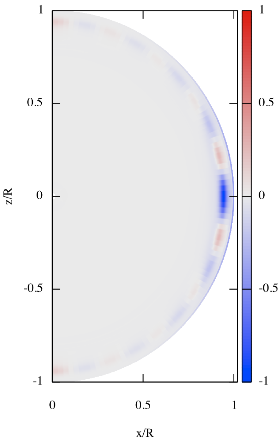
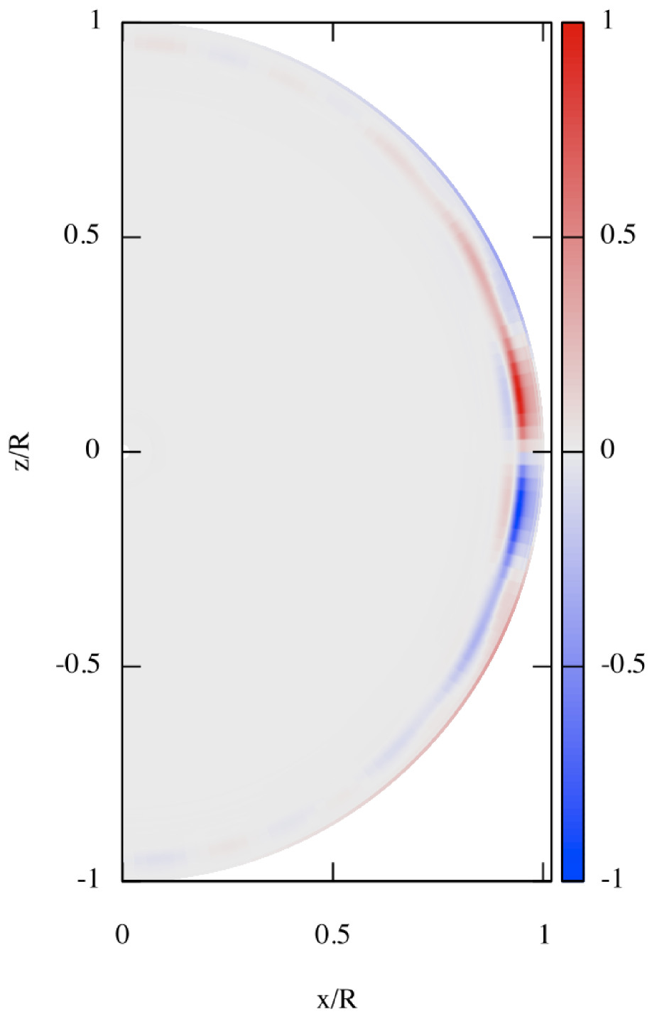
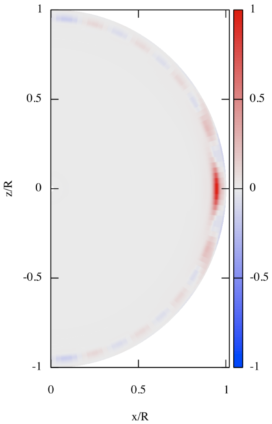
Figure 2: Top: second-order perturbations $u_{S,k}\equiv\hat{v}_{S,l_{k}}^{(2)}/R\sigma_{0}$, $u_{H,k}\equiv\hat{v}_{H,l_{k}}^{(2)}/R\sigma_{0}$, and $u_{T,k}\equiv\hat{v}_{T,l_{k}}^{(2)}/R\sigma_{0}$ as a function of $r/R$ for the even retrograde $g_{64}$-mode of $l=|m|=2$ of a $6M_{\odot}$ main sequence star model at $\bar{\Omega}=0.1$, where the solid lines, dash-dotted lines, dashed lines, long dashed lines, and dotted lines represent respectively the components corresponding to $k=1,~{}3,~{}5,~{}7$, and $9$. Bottom: density maps of the functions $v_{r}^{(2)}(r,\theta)/R\sigma_{0}$, $v_{\theta}^{(2)}(r,\theta)/R\sigma_{0}$, and $v_{\phi}^{(2)}(r,\theta)/R\sigma_{0}$ for the mode. The functions are normalized by their maximum amplitudes. Red and blue colors correspond to positive and negative values, respectively.

3.1 Slowly Pulsating B-type Stars

In SPB stars, low frequency $g$- and $r$-modes are excited by the opacity bump mechanism (Dziembowski et al. 1993; Gautschy & Saio 1993; Lee 2006; Aprilia et al. 2011). Here, we calculate mean flows driven by unstable low frequency $g$- and $r$-modes of a $6M_{\odot}$ main-sequence star, whose physical parameters are typical of a SPB star: $\log(L/L_{\odot})=3.2328$, $\log T_{\rm eff}=4.1982$, $R/R_{\odot}=5.55$, and $X_{c}=0.1237$, $X=0.7$, and $Z=0.02$. Because good numerical consistency in the sense discussed in §2.4 is attained only for $\bar{\Omega}<\kern-11.99998pt\lower 4.73611pt\hbox{$\sim$}0.1$ for the $g$-modes, we restrict our discussion of $g$-modes to the case of $\bar{\Omega}=0.1$. Since most of the unstable $g$-modes of the SPB model have frequencies $|\bar{\omega}|>\kern-11.99998pt\lower 4.73611pt\hbox{$\sim$}~{}\bar{\Omega}$ for $\bar{\Omega}\sim 0.1$, we can use the expansion length $j_{\rm max}\sim 5$ to obtain sufficiently accurate eigenfunctions, and we set $k_{\rm max}=10$ for second order perturbation calculations.

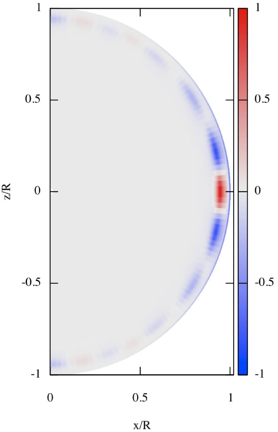
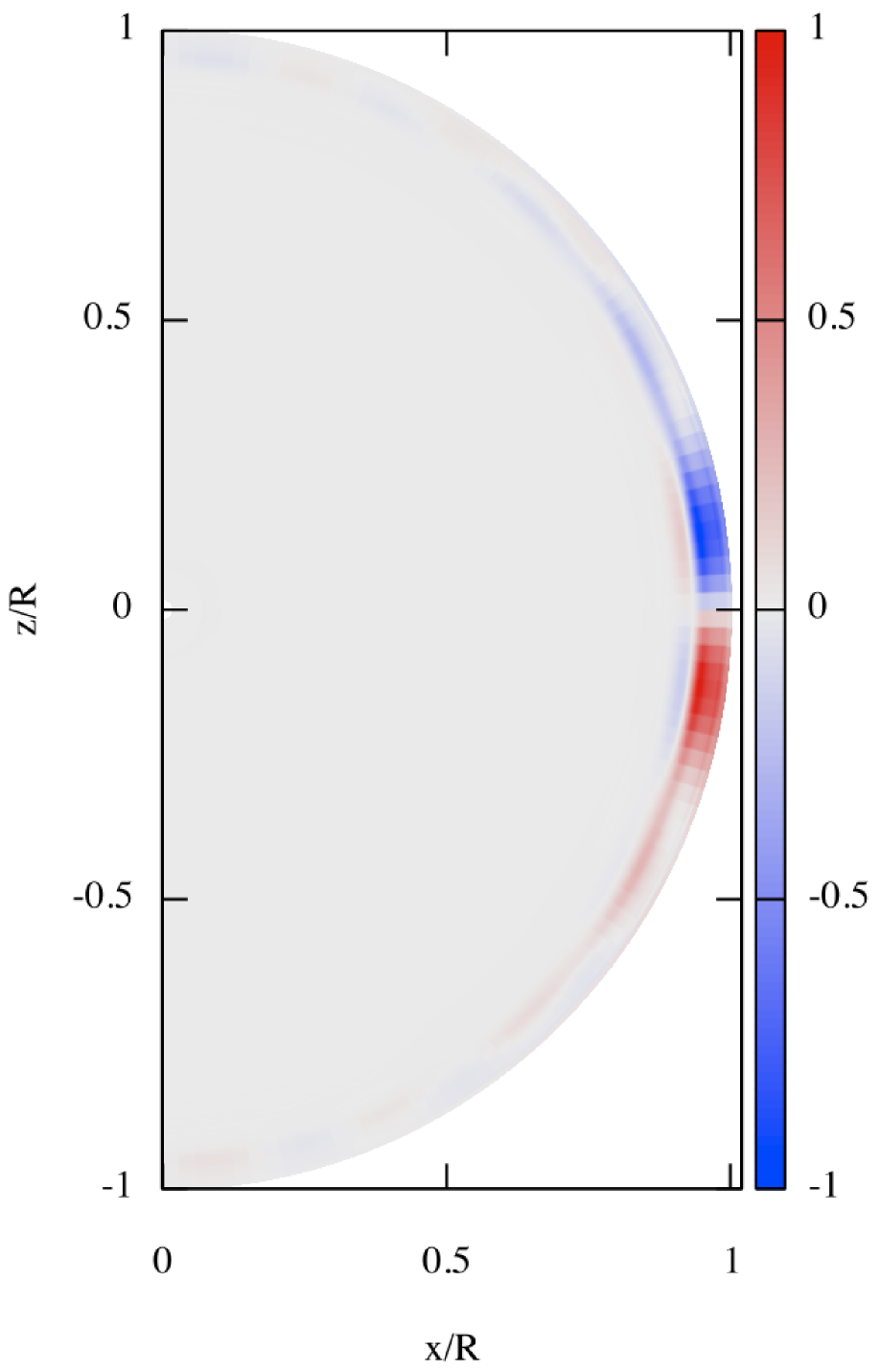
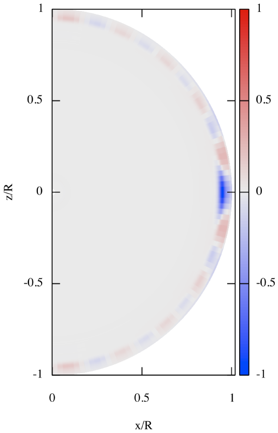
Figure 3: Same as Figure 2 but for the even prograde $g_{30}$-mode of $l=|m|=2$.

3.1.1 $g$-modes

Let us first discuss mean flows driven by low frequency $g$-modes. As numerically shown by Aprilia et al. (2011), both prograde and retrograde low frequency $g$-modes are excited by the opacity bump mechanism in rapidly rotating SPB stars. Most of $l=|m|$ retrograde $g$-modes of the star, that would be unstable if the star were non-rotating, are stabilized by rapid rotation as a result of their coupling with stable $l>|m|$ $g$-modes. As a consequence, only a small number of them survive as unstable modes in rapidly rotating SPB stars. This is not the case of prograde $l=|m|$ $g$-modes and most of them remain unstable even at rapid rotation.

In Figure 2, we plot, in the top panels, the expansion coefficients $u_{S,k}\equiv\hat{v}_{S,l_{k}}^{(2)}/R\sigma_{0}$, $u_{H,k}\equiv\hat{v}_{H,l_{k}}^{(2)}/R\sigma_{0}$, and $u_{T,k}\equiv\hat{v}_{T,l_{k}}^{(2)}/R\sigma_{0}$ as a function of $r/R$ for the even retrograde $g_{30}$-mode of $l=|m|=2$ for $\bar{\Omega}=0.1$, where the normalized eigenfrequency $\bar{\omega}\equiv\omega/\sigma_{0}$ is $\bar{\omega}=(0.4672,-5.7\times 10^{-6})$. Here, the amplitude normalization of the linear mode is given by $S_{l_{1}}=1$ at the surface. Note that $l=|m|$ implies the mode is an even mode. As shown by Figure 1, the functions $u_{S,k}$, $u_{H,k}$, and $u_{T,k}$ have large amplitudes only in the outer envelope layers. Note also that the peaks of the functions at $r/R\sim 0.95$ correspond to the place at which the mode excitation strongly occurs. The reason for this behavior is that, in addition to the fact that mode amplitudes can be large near the surface because of low density, thermal diffusion grows below the surface of upper main-sequence stars. Therefore, deposition/extraction of momentum may take place in these layers (e.g., Lee et al. 2014). These wave-mean flow interactions thus drive both zonal and meridional flows there (see e.g. Mathis et al. 2013 in the case of low-mass stars). The amplitude of the zonal component $u_{T,k}$ is much larger than those of the meridional ones, $u_{S,k}$ and $u_{H,k}$, by several orders of magnitude. Therefore, the kinetic energy of the induced azimuthal rotational motion is larger than that of generated meridional circulation.

The reason that the azimuthal flow is much larger than the radial/latitudinal flows can be simply understood from the propagation of the mode pattern. A purely adiabatic non-axisymmetric mode is a standing wave in both the radial and latitudinal directions. However, the mode propagates around the equator of the star and can be thought of as a traveling wave in the azimuthal direction. Consequently, the mean flows created by the wave are much larger in the azimuthal direction, because the traveling wave propagates in one direction (either prograde or retrograde). In the radial/latitudinal direction, the standing wave, which is composed of traveling waves propagating in opposite directions, contains components that cancel each other out such that there is no net flow in these directions. In other words, since the modes contain angular momentum only in the z-direction, the flows they induce are only in the azimuthal direction. For a weakly non-adiabatic mode such as those discussed here, the modes also produce non-zero mean flows in the radial/latitudinal directions. However, the azimuthal flows will still be much larger.

Figure 2 also shows for the $g_{30}$-mode the density maps of the components $v_{r}^{(2)}(r,\theta)/R\sigma_{0}$, $v_{\theta}^{(2)}(r,\theta)/R\sigma_{0}$, and $v_{\phi}^{(2)}(r,\theta)/R\sigma_{0}$, in the bottom panels, where these functions, which depend on both radial distance and latitude, are normalized by their maximum amplitudes. The vertical axis is the rotation axis ($x=y=0$), and the equatorial plane is given by $z=0$. The radial and the azimuthal velocity components ($v_{r}^{(2)}(r,\theta)/R\sigma_{0}$ and $v_{\phi}^{(2)}(r,\theta)/R\sigma_{0}$) are symmetric about the equator, while the latitudinal one ($v_{\theta}^{(2)}(r,\theta)/R\sigma_{0}$) is antisymmetric. As shown by the maps for the retrograde $g_{30}$ mode, the pulsation driven mean flows near the surface have the velocity components $v_{\theta}^{(2)}$ toward the equatorial plane and the component $v_{r}^{(2)}$ heading inwards. The $\phi$ component $v_{\phi}^{(2)}$ is positive, indicating acceleration of the rotation near the equatorial surface. As suggested by the density maps, the amplitudes of pulsation driven mean flows tend to be confined in the equatorial region. This reflects the properties of low frequency modes of rotating stars, that is, their amplitudes are also confined in the equatorial region, particularly for rapidly rotating case (see, e.g., Berthomieu et al 1978; Bildsten et al 1996, Lee & Saio 1997; Townsend 2003ab).

We see that pulsations induce a differential rotation $\delta\Omega\left(r,\theta\right)=v_{\phi}^{(2)}(r,\theta)/(r\sin\theta)$, which is a function of both radial distance and latitude. This is the signature of pulsation-driven transport of angular momentum both in the vertical and in the horizontal directions (e.g., Mathis 2009). It is the first time that such wave-driven differential rotation is computed in 2-D. Indeed, previous computations treated reduced cases of the radial shellular rotation (e.g., Talon & Charbonnel 2005; Mathis et al. 2013) or focused on the dynamics in the equatorial plane (e.g., Rogers et al. 2013). Like in previous computations performed for low-mass stars by Talon & Charbonnel (2005) and Mathis et al. (2013), we see in massive stars that the meridional circulation can be multicellular both in radius and in latitude. These patterns differ from properties of meridional circulations driven by large-scale differential rotation in models where waves are not taken into account. Such a computation is of interest for development of 2-D models of rotating stars (Rieutord 2006), in which waves must be taken into account in a near future. In the case of the $g_{30}$-mode, the amplitudes of the functions are confined in the equatorial regions. In the context of active massive stars, such as Be stars, it is interesting to note that for the retrograde mode, the velocity perturbations $v_{\phi}^{(2)}$ at the surface becomes positive in the narrow equatorial region, while $v_{r}^{(2)}$ is negative. The positive zonal component can then help the surface layers to reach the critical angular velocity needed to eject matter in the circumstellar environment.

In Figure 3, we show, in the top panels, the expansion coefficients $u_{S,k}$, $u_{H,k}$, and $u_{T,k}$ for the even prograde $g_{30}$-mode of $l=|m|=2$ at $\bar{\Omega}=0.1$, for which $\bar{\omega}=(0.4025,-7.9\times 10^{-6})$. The corresponding 2-D density maps of the velocity components $v_{r}^{(2)}(r,\theta)/R\sigma_{0}$, $v_{\theta}^{(2)}(r,\theta)/R\sigma_{0}$, and $v_{\phi}^{(2)}(r,\theta)/R\sigma_{0}$ are given in the bottom panels in the same figure. As in the previous case, the functions $u_{S,k}$, $u_{H,k}$, and $u_{T,k}$ have large amplitudes only in the outer surface layers. As in the previously studied case of the retrograde $g_{30}$-mode, the amplitude of $u_{T,k}$ is much larger than those of $u_{S,k}$ and $u_{H,k}$. From these density maps, the flow patterns driven by the prograde $g_{30}$-mode in the surface equatorial region is opposite to those by the retrograde $g_{30}$ mode, that is, the radial velocity $v_{r}^{(2)}$ is towards the surface and the components $v_{\theta}^{(2)}$ show flows out of the equatorial plane. This different behavior between retrograde and prograde $g$-modes shows that it is necessary to sum over all the modes that are excited in a given star to be able to understand the total wave-driven zonal and meridional mean flows and their net effect. This is the reason why $r$- and $p$- modes have also to be considered.

3.1.2 $r$-modes

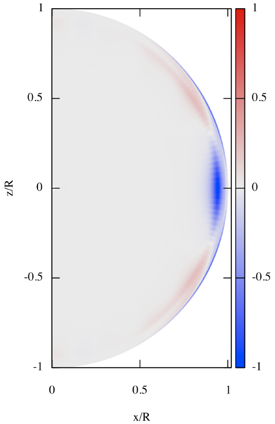
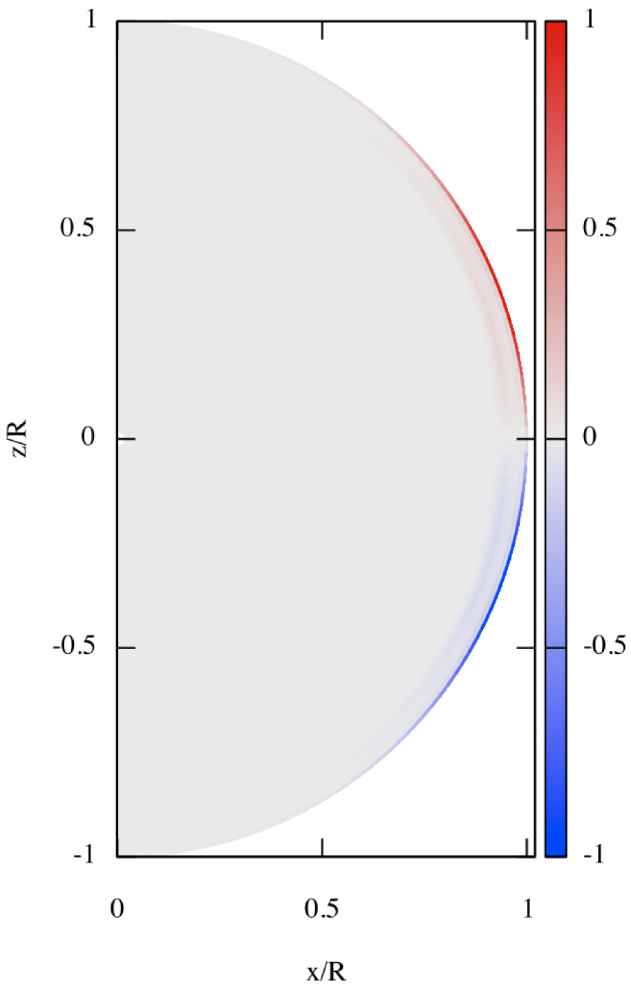
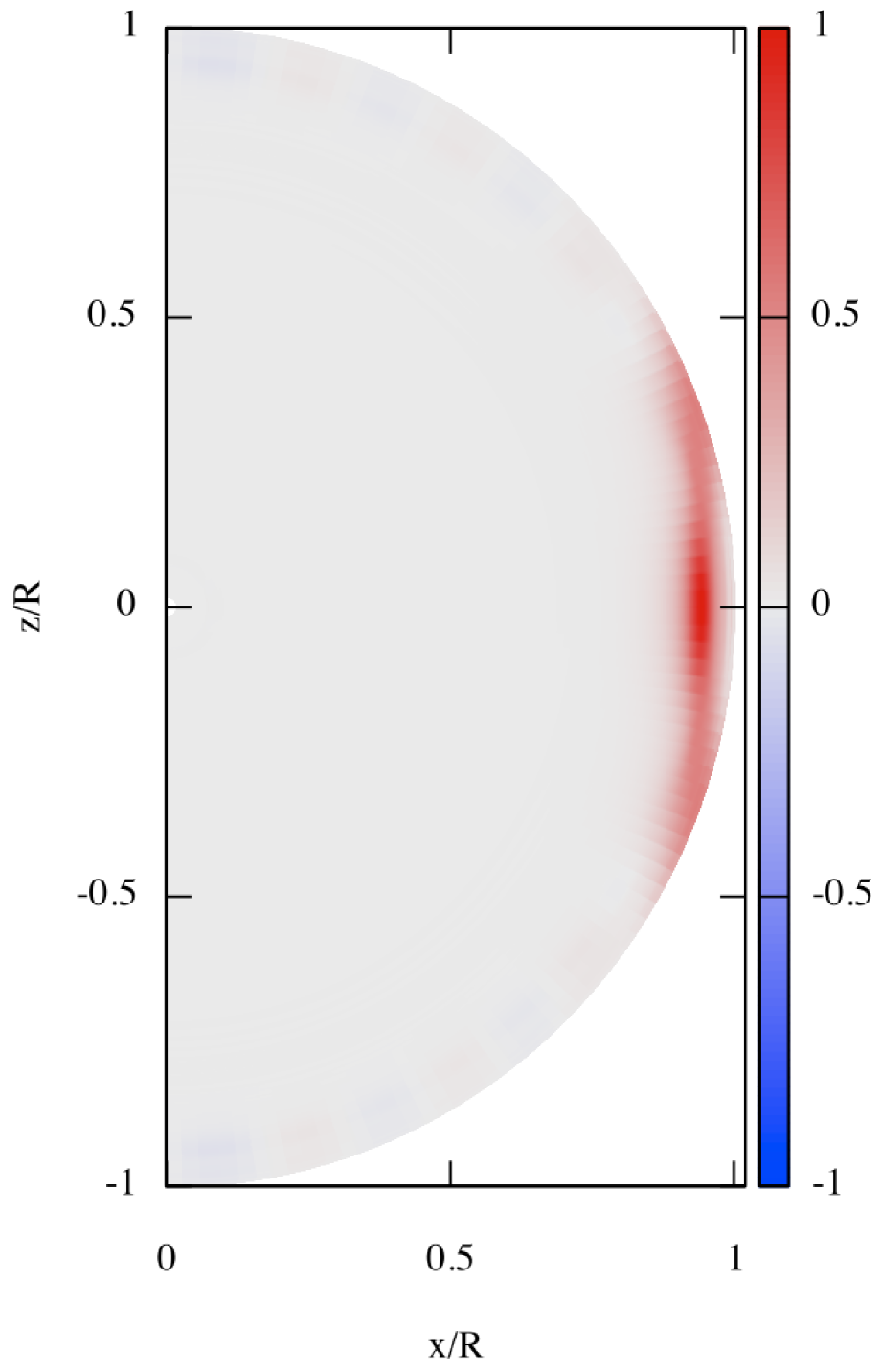
Figure 4: Same as Figure 2 but for the $l^{\prime}=|m|=2$ odd $r_{36}$-mode at $\bar{\Omega}=0.4$.

$r$-modes are rotationally induced retrograde modes and constitute a subclass of inertial modes, for which the Coriolis acceleration is the restoring force. In the slow rotation limit (i.e., $\Omega\rightarrow 0$), $r$-modes associated with the degree $l^{\prime}$ and the azimuthal index $m$ have an asymptotic co-rotating frame frequency given by $\omega=2m\Omega/\left[l^{\prime}(l^{\prime}+1)\right]$, and the displacement vector $\xi$ is dominated by its toroidal component $\left({\rm i}T_{l^{\prime}}\right)$. Since numerous $l^{\prime}=|m|$ $r$-modes of odd parity are also excited by the opacity bump mechanism in SPB stars (e.g., Lee 2006), it is necessary to examine how $r$-modes drive mean flows in rotating SPB stars.

The top panels of Figure 4 show the expansion coefficients $u_{S,k}$, $u_{H,k}$, and $u_{T,k}$ as a function of $r/R$, while the bottom panels of the figure give the corresponding 2-D density maps of the three components $v_{r}^{(2)}(r,\theta)/R\sigma_{0}$, $v_{\theta}^{(2)}(r,\theta)/R\sigma_{0}$, and $v_{\phi}^{(2)}(r,\theta)/R\sigma_{0}$ for the odd $r_{36}$-mode of $l^{\prime}=m=2$ at $\bar{\Omega}=0.4$, for which $\bar{\omega}=(0.2199,-2.1\times 10^{-6})$. As in the case of g-modes, the amplitudes of the expansion coefficients become large in the outer envelope. Moreover, the zonal flow ($u_{T,k}$) is still much larger than the meridional one (given by $u_{S,k}$ and $u_{H,k}$). As shown by the 2-D density maps, gross flow patterns driven by the $r$-mode are similar to those by the retrograde $g_{30}$-mode, although the zonal acceleration near the surface is much more prominent than that for the retrograde $g$-mode.

3.1.3 Lagrange velocity perturbations

The vertical Lagrangian velocity perturbation $\delta v_{r}^{(2)}$ can be an important quantity when we consider radial transport of gaseous matter in the interior of stars. In Figure 5, we show the 2-D density maps of $\delta v_{r}^{(2)}/R\sigma_{0}$ for the even retrograde and prograde $g_{30}$-modes of $l=|m|=2$ at $\bar{\Omega}=0.1$ and for the odd $r_{36}$-mode of $l^{\prime}=|m|=2$ at $\bar{\Omega}=0.4$. Comparing the bottom left panels of Figures 2, 3, and 4 with the corresponding ones in Figure 5, we see that there appear no essential differences between $v_{r}^{(2)}$ and $\delta v_{r}^{(2)}$ for the low frequency modes. When zonal flows in the surface equatorial layers are accelerated by the retrograde modes, the radial flows are driven inwards.

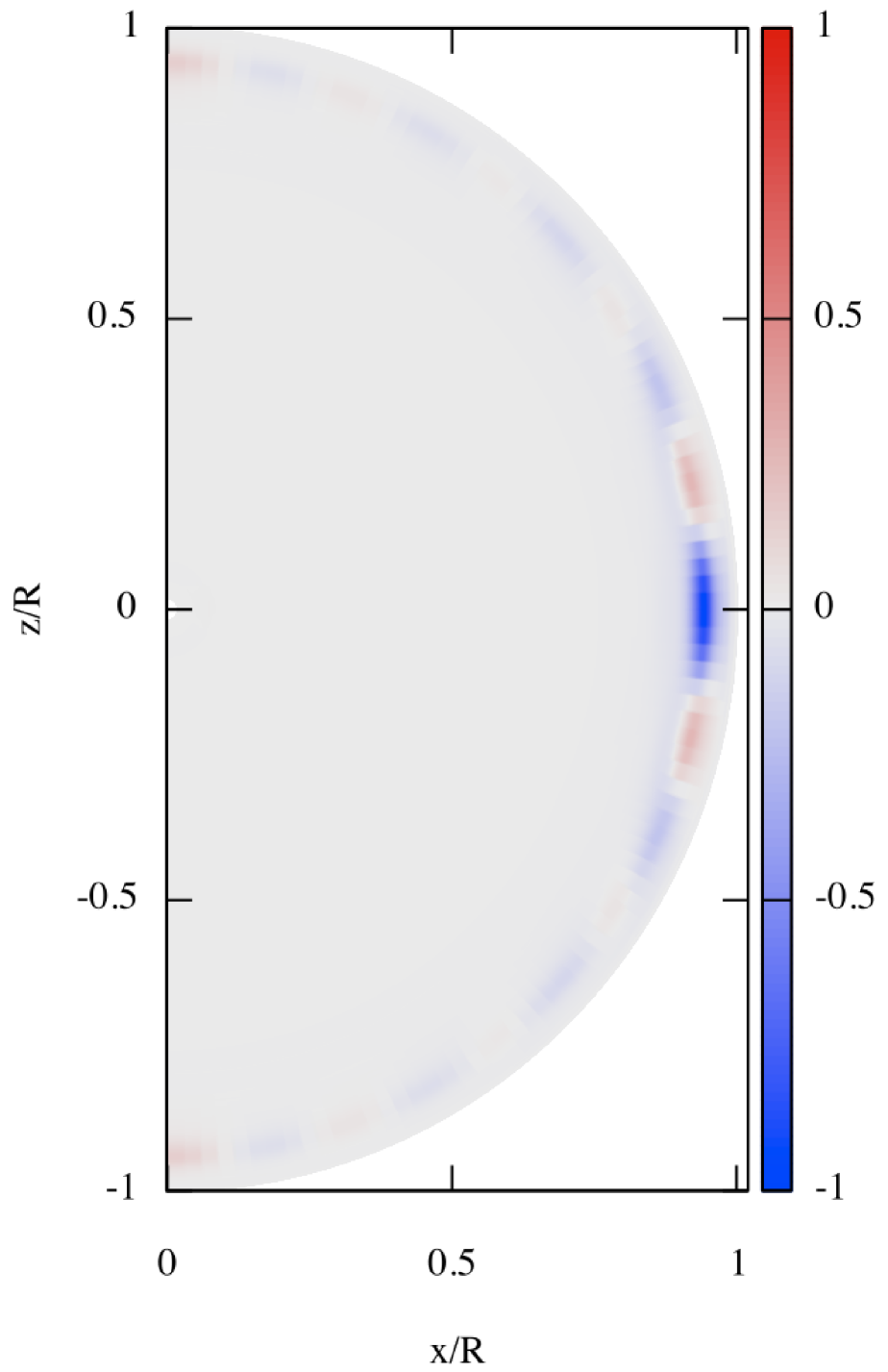
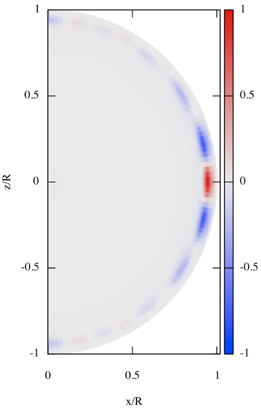
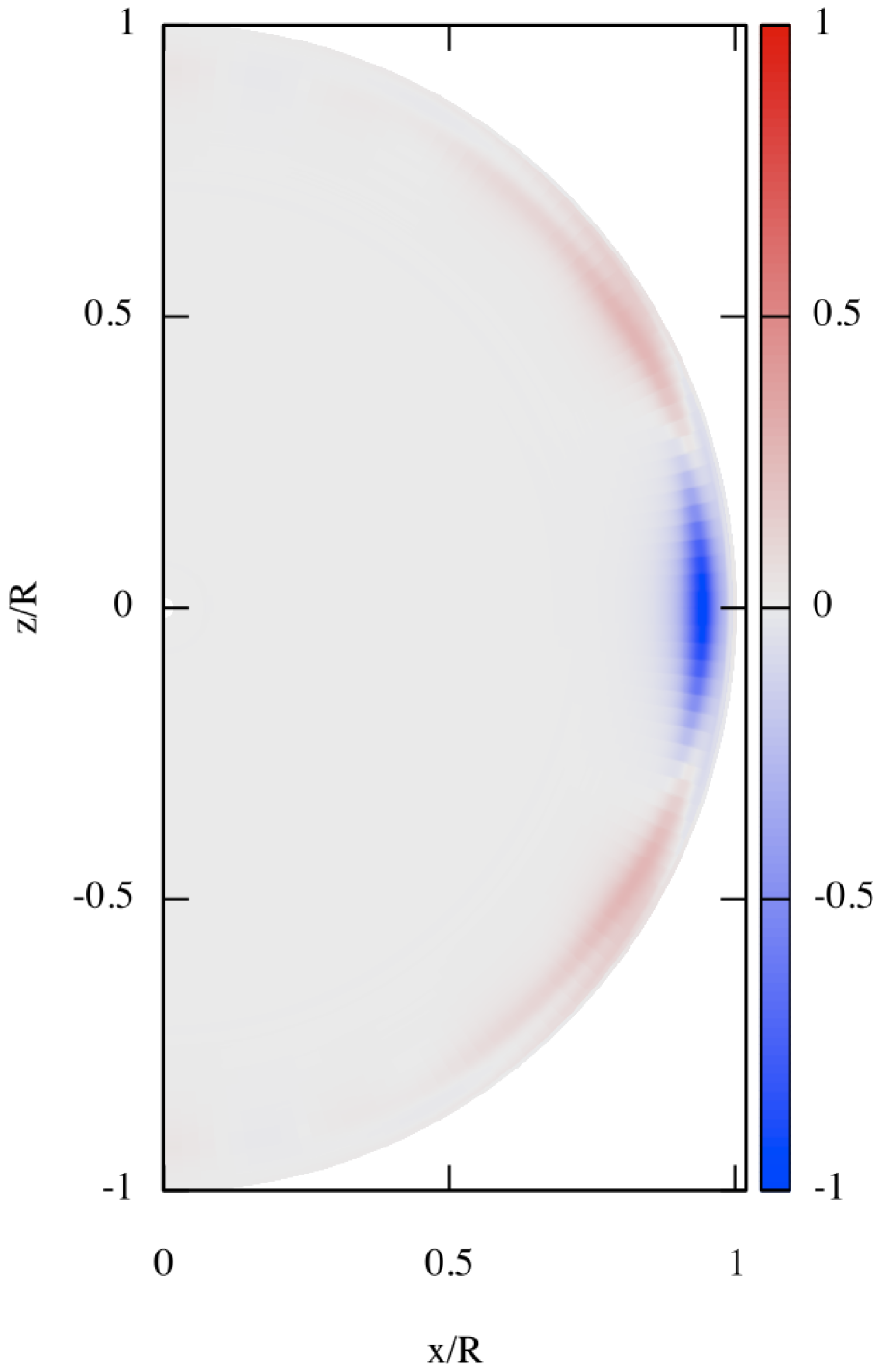
Figure 5: Density maps of the functions $\delta v_{r}^{(2)}(r,\theta)/r\sigma_{0}$, from left to right panels, for the retrograde $g_{30}$-mode and the prograde $g_{30}$-mode of $l=|m|=2$ at $\bar{\Omega}=0.1$, and for the $l^{\prime}=|m|=2$ $r_{36}$-mode at $\bar{\Omega}=0.4$ for the $6M_{\odot}$ main sequence model. The functions are normalized by their maximum amplitudes. Red and blue colors correspond to positive and negative values respectively.

3.2 $\beta$ Cephei stars

In addition to exciting $g$- and $r$-modes in cool B stars (SPB stars), the iron opacity bump mechanism also excites $p$-modes in hotter B stars ($\beta$ Cephei stars). We calculate mean flows driven by unstable low radial order $p$-modes of a $15M_{\odot}$ main-sequence model, whose physical parameters are typical of a $\beta$ Cep star: $\log(L/L_{\odot})=4.5928$, $\log T_{\rm eff}=4.394$, $R/R_{\odot}=10.8$, and $X_{c}=0.130$. For this model, $l=|m|$ low radial oder modes with normalized frequency $\bar{\omega}$ between 2 and 5 become pulsationally unstable. Since the method of calculation used in this paper for $p$-modes of rotating stars is not necessarily appropriate for very rapid rotation $\bar{\Omega}\sim 1$, as suggested by full 2-D computations of $p$-modes in rapidly rotating stars (Lignières et al. 2006; Reese et al. 2006), we restrict the present discussion to the case of slow rotation rates $\bar{\Omega}\sim 0.1$.

Figure 6 and 7 are respectively for the retrograde $l=m=2$ $p$-mode of $\bar{\omega}=(2.584,-7.9\times 10^{-7})$ and for the prograde $l=|m|=2$ $p$-mode of $\bar{\omega}=(2.634,-4.5\times 10^{-7})$. Note that, if we count the number of radial nodes of the eigenfunction $S_{l_{1}}$ in the way described in Unno et al (1989), we obtain $k\equiv n_{p}-n_{g}=-3$, suggesting that the mode should be classified as a $g_{3}$-mode, where $n_{g}$ and $n_{p}$ are the numbers of $g$-type and $p$-type nodes of the eigenfunction $S_{l_{1}}$. However, we simply call these modes a $p$-mode because it behaves as a $p$-mode in the envelope.

As shown by Figures 6 and 7, and as in the case of SPB stars studied above, the zonal component ($u_{T,k}$) is dominant over meridional ones ($u_{S,k}$ and $u_{H,k}$). The flow patterns $v_{r}^{(2)}$ and $v_{\theta}^{(2)}$ in the surface layers are quite similar between the retrograde and prograde $p$-modes, which is contrary to the case of low frequency $g$-modes. This is because the Coriolis terms proportional to $m\Omega/\omega$ are not important to determine these velocity components. Zonal acceleration in the surface equatorial region occurs for the retrograde mode, although deceleration takes place for the prograde mode. The Lagrangian velocity perturbations $\delta v_{r}^{(2)}$ of the $p$-modes are depicted in Figure 8, which shows that the additional terms $\overline{v_{i;j}^{(1)}\xi_{j}}$ can be significant enough, that is, even if $v_{r}^{(2)}$ is positive in the surface equatorial region, $\delta v_{r}^{(2)}$ becomes negative.

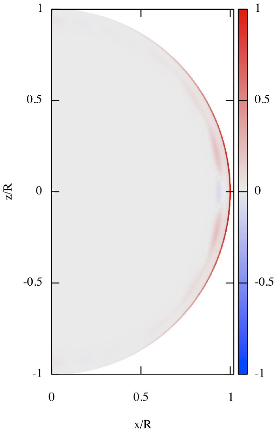
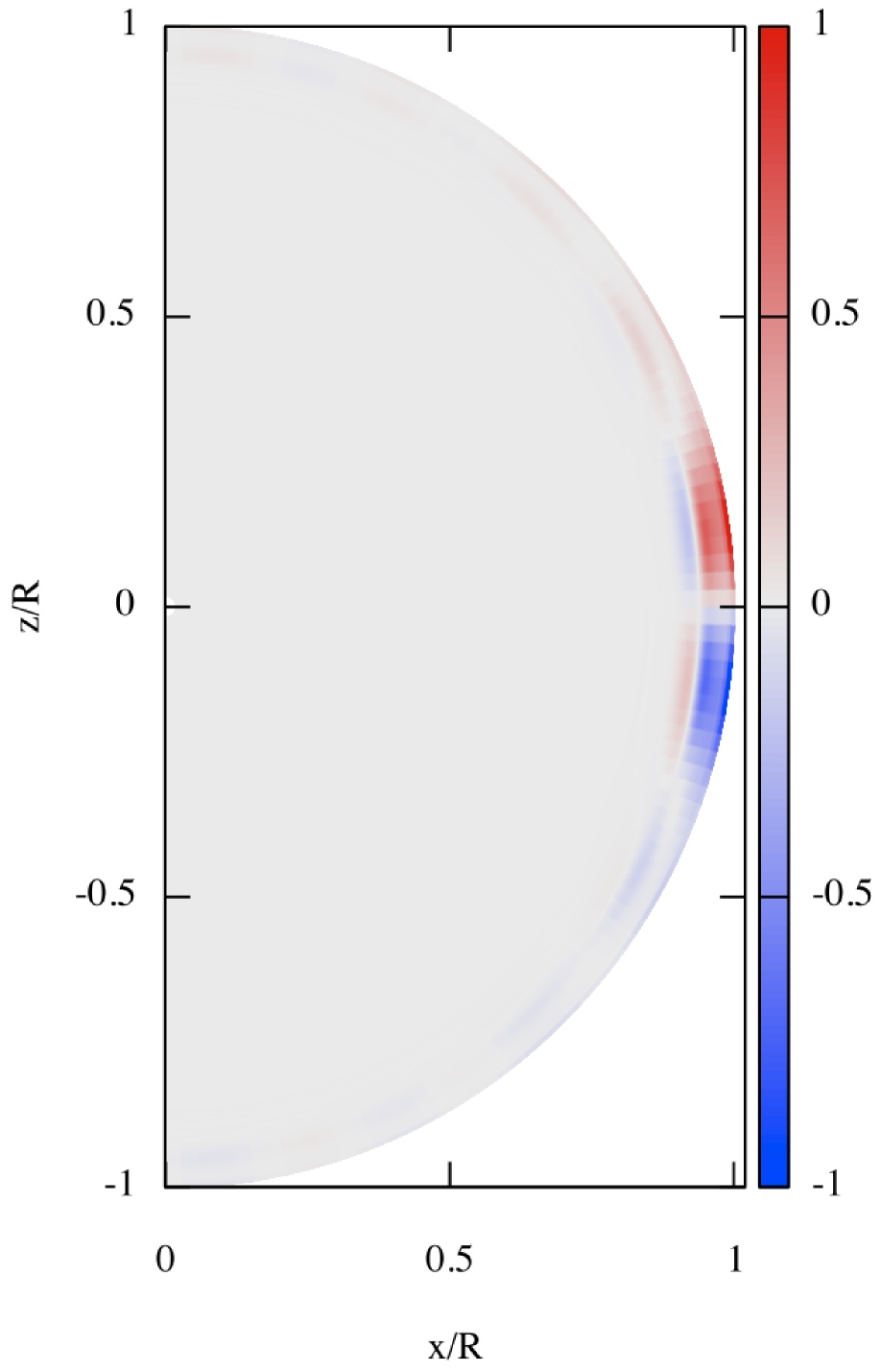
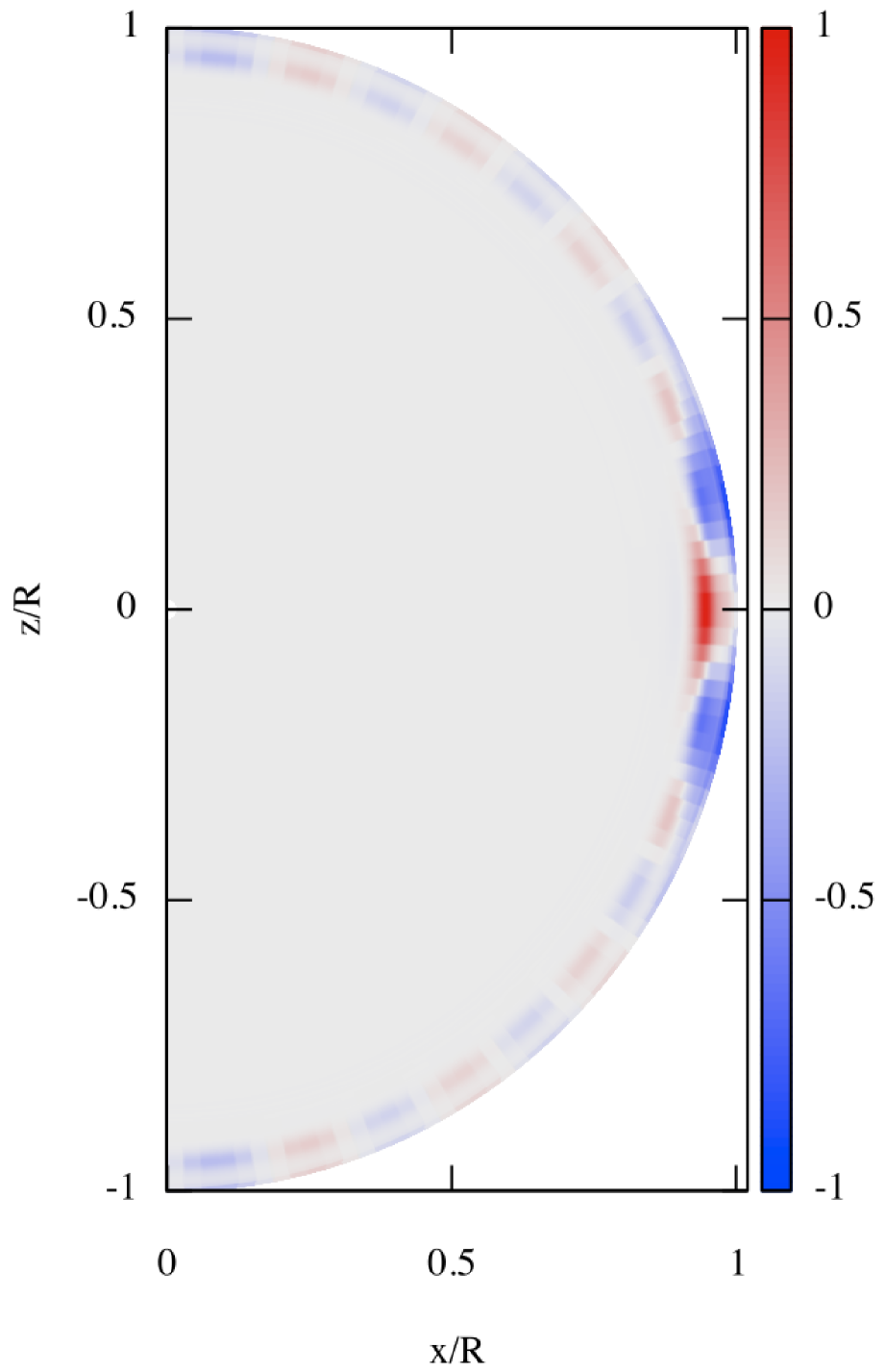
Figure 6: Same as Figure 2 but for the $l=|m|=2$ even retrograde $p$-mode of the $15M_{\odot}$ main sequence star model where $\bar{\Omega}=0.1$.

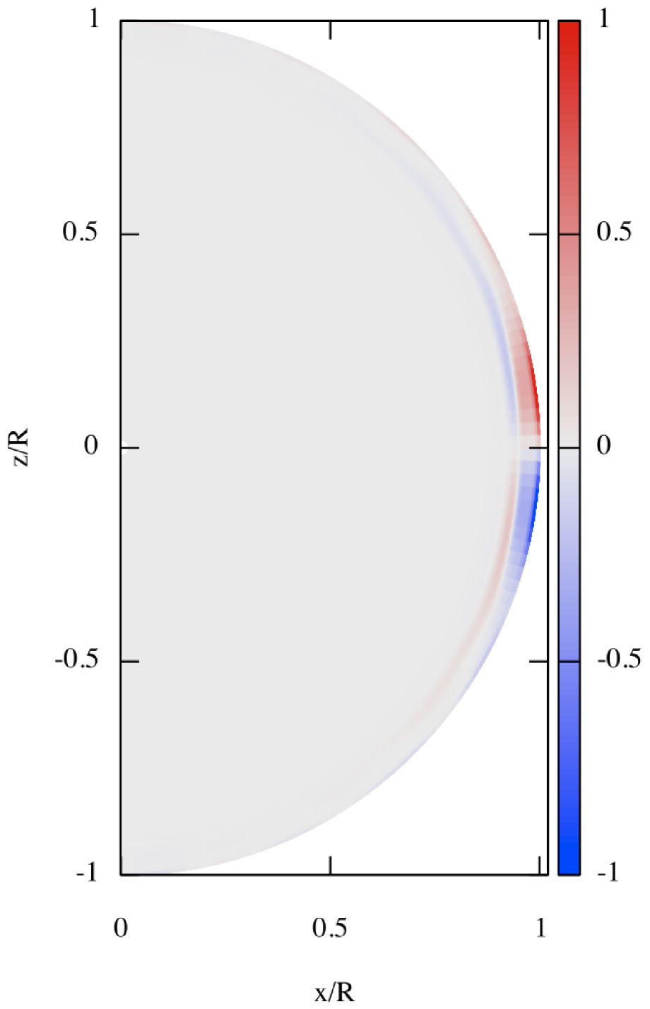
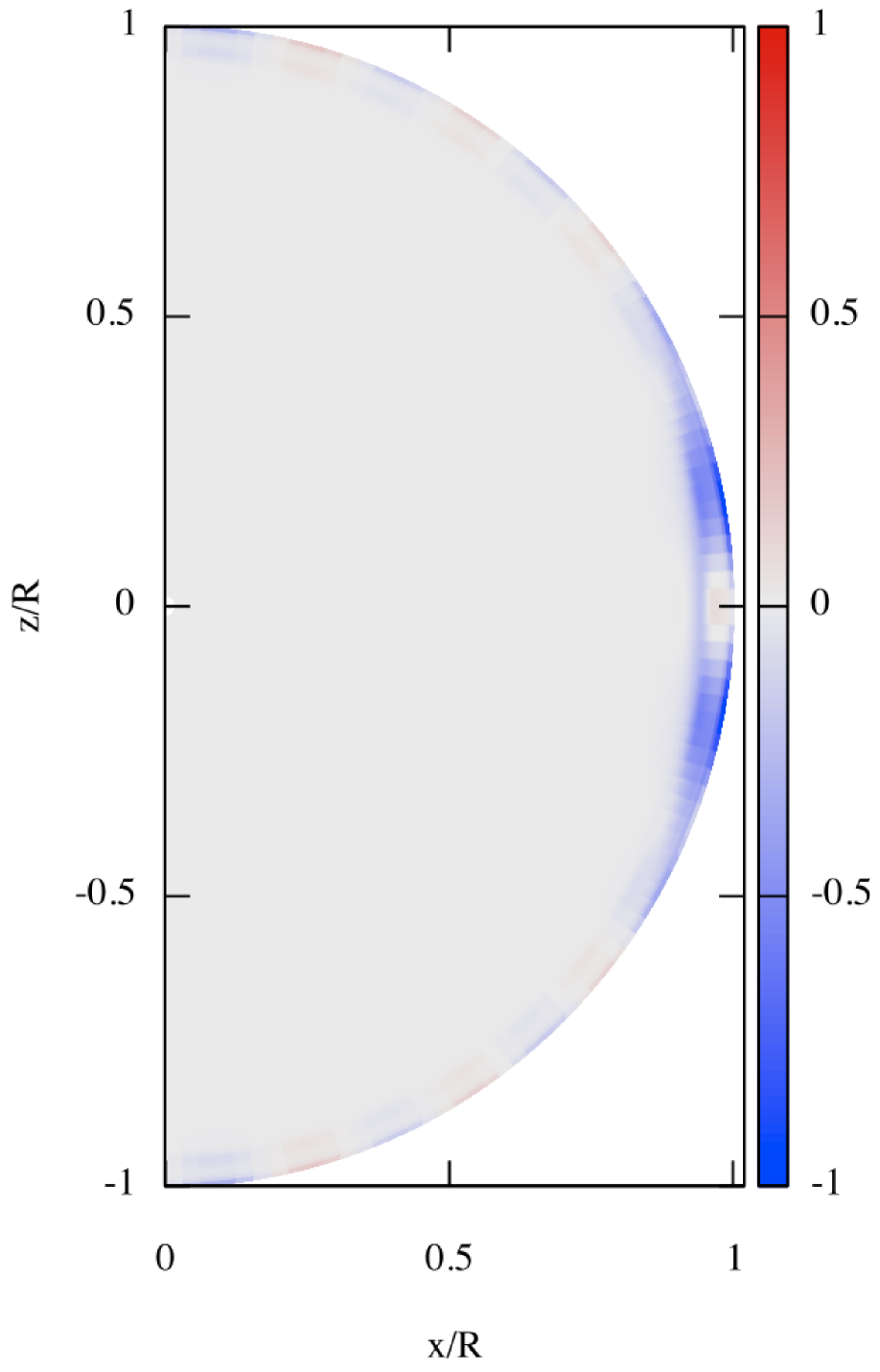
Figure 7: Same as Figure 6 but for the $l=|m|=2$ even prograde $p$-mode.

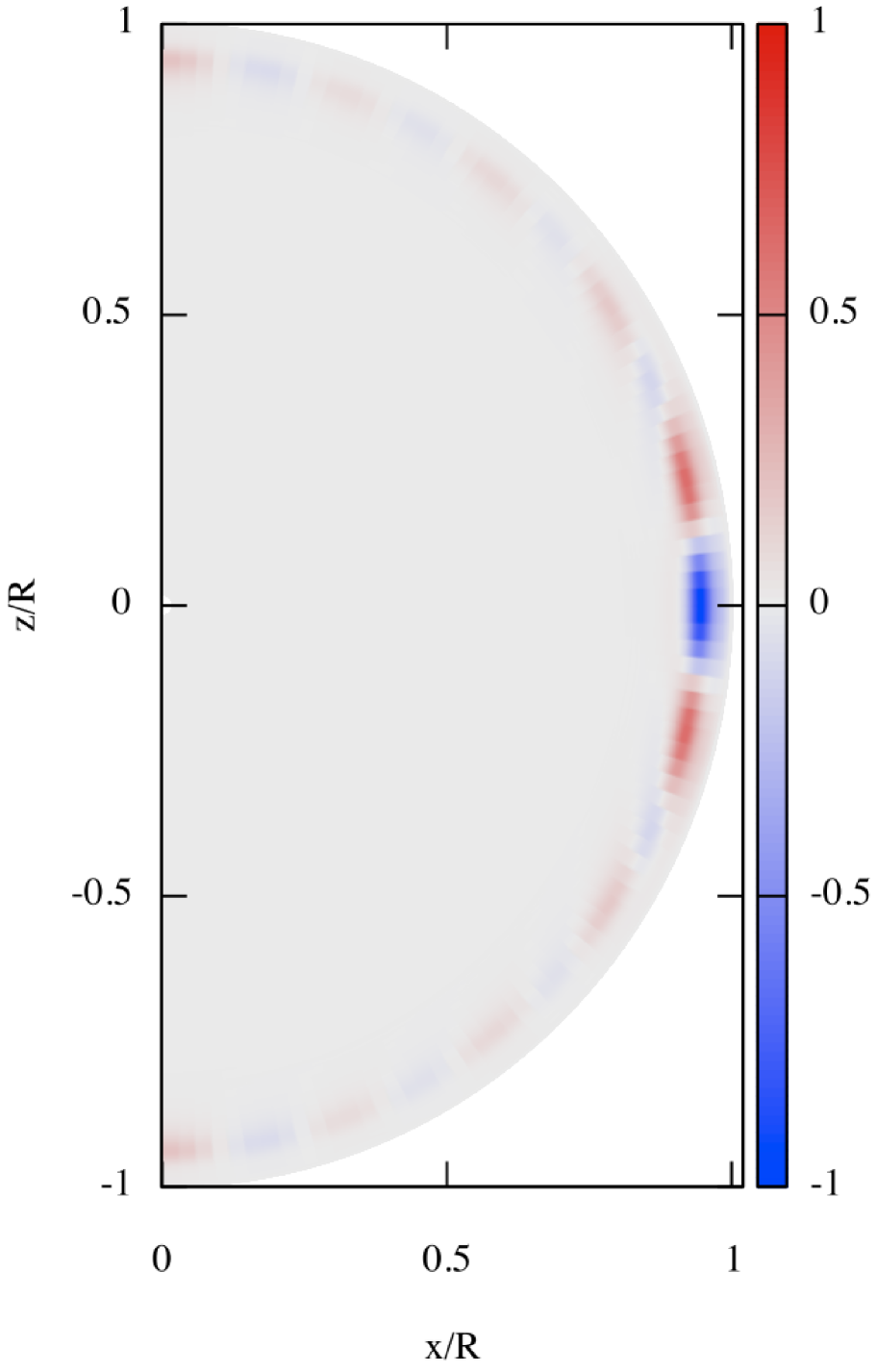
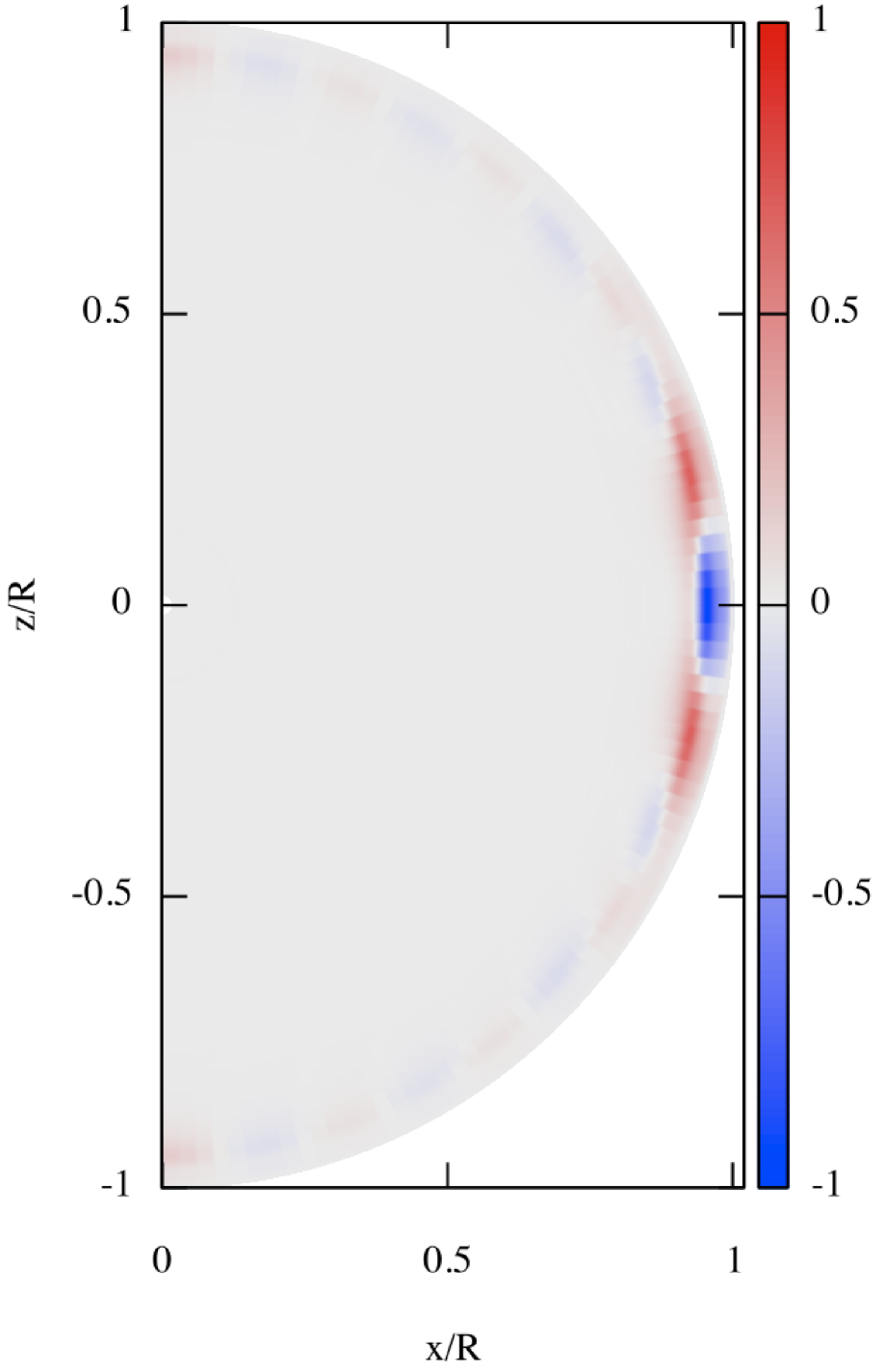
Figure 8: Same as Figure 5 but for even retrograde and prograde $p$-modes of $l=|m|=2$ of the $15M_{\odot}$ main sequence star model where $\bar{\Omega}=0.1$.

4 Discussion and Conclusion

Figure 9: $\cal L$ (dashed line) and $\cal R$ (solid line) for the $g_{30}$-mode and $r_{36}$-mode of the SPB star model and for the $p$-mode of the $\beta$ Cephei star model, from left to right panels, where we use $\bar{\Omega}=0.1$ for the $g$- and $p$-modes and $\bar{\Omega}=0.4$ for the $r$-mode.

As a consistency cheque of our mean flow computations, in Figure 9 we plot the functions $\cal L$ and $\cal R$ for the prograde $p$- and $g$-modes, and the retrograde $r$-modes depicted in Figure 1. Note that equation (62) is well satisfied for these modes. The two functions agree very well for the $g$- and $p$-modes, but they show disagreement in the outer most layers for the $r_{36}$-mode. Although the reason of the disagreement for the $r$-mode is not well understood, possible reasons might be that the number of radial nodes of the eigenfunctions is large, which makes it difficult to correctly compute the eigenfunctions, and that the toroidal components of the displacement vector are significantly dominant over the the other components although equation (62) is determined by the phase differences between the less dominant eigenfunctions.

Assuming an initial uniform rotation, we have derived the governing equations for zonal and meridional axisymmetric mean flows driven by unstable non-axisymmetric oscillation modes in rapidly rotating massive main-sequence stars, where the magnitude of mean flows are assumed to be of second-order of the oscillation amplitudes. The governing equations are a set of coupled linear ordinary differential equations for the second-order quantities with inhomogeneous terms, coming from products of the eigenfunctions of linear oscillation modes. To demonstrate the applicability of the formalism and its importance for astrophysical studies, we have computed zonal and meridional axisymmetric mean flows driven by non-axisymmetric $g$- and $r$-modes in SPB stars and $p$-modes in $\beta$ Cephei stars, where oscillation modes are assumed to be excited by the iron opacity bump mechanism.

For most of the oscillation modes considered in this paper, these mean flows have large amplitudes only in the surface regions of the stars, particularly in the regions where the oscillation modes are excited. The first interesting point to note is that for low frequency retrograde $g$-modes and $r$-modes excited by the opacity bump mechanism, $v_{\phi}^{(2)}$ can be positive in the surface equatorial regions, indicating that surface fluid elements could be accelerated in the same direction as the surface stellar rotation. The velocity fields generated in the surface layers are related to the Reynolds stresses of the waves and transported fluxes that drive exchanges between waves (oscillations) and zonal and meridional mean flows (e.g., Bretherton 1969; Andrews & McIntyre 1978a; Holton 1982; Mathis et al. 2013; Belkacem et al. 2015a). For the zonal component, we provide for the first time the 2-D geometry of the wave-driven differential rotation given by $v_{\phi}^{(2)}(r,\theta)/\left(r\sin\theta\sigma_{0}\right)$. This provides us with information on the transport of angular momentum by waves both in the vertical and in the latitudinal directions (e.g., Andrews & McIntyre 1978a; Mathis 2009).

Moreover, we computed for the first time 2-D wave-driven meridional circulation. It can have multi-cellular pattern in the radial direction, while its latitude-dependence depends on the studied modes. If we use Eq. (1) to roughly estimate the magnitude of the rotationally-driven meridional circulation, we have $v_{r:\rm MC}/R\sigma_{0}\sim 10^{-7}\times\bar{\Omega}^{2}$ for a $10M_{\odot}$ ZAMS star. This number suggests that pulsation-driven mean meridional flows have comparable magnitude to rotationally-driven meridional circulation if the oscillation modes have amplitudes $S_{l_{1}}\sim 10^{-4}$ to $10^{-3}$ at the surface, depending on the mode. To estimate the magnitudes of velocity fields of pulsation-driven mean flows, we need to theoretically estimate the amplitudes of pulsation, which has always been a difficult problem. One possible way to estimate oscillation amplitudes for the $\kappa-$mechanism is to employ a weak non-linear theory of oscillations (see e.g., Lee 2012), although it is another very difficult task to apply this theory to oscillation modes in rapidly rotating stars. As suggested by Lee (2012), the amplitudes of this magnitude $S_{l_{1}}\sim 10^{-4}$ to $10^{-3}$ is probably attainable in SPB stars. This is the reason why wave-driven mean zonal and meridional mean flows must be taken into account when studying the evolution of rotating massive stars, as it is done for low-mass stars (e.g., Talon & Charbonnel 2005; Mathis et al. 2013).

In this paper, we have applied several simplifying assumptions to make the formulation and calculation of mean flows tractable. First, we used the radiative transfer equation to derive the governing equation for the second-order variables, even for convective regions in the interior. This crude treatment may be justified for massive main-sequence stars having only weak surface convection layers, but may not be justified for low-mass stars with thick surface convection zones. Note that $\kappa$-driven pulsations do not have any contribution to mean flow in the convective core of massive stars, unless the effect of the viscous force on inertial modes is taken into account. However, the induced transport of momentum is negligible compared to transport by convective eddies (Browning et al. 2004). In addition, we ignored the effects of centrifugal force on the equilibrium structure, oscillation calculation, and mean flow computation for rapidly rotating stars. This neglect of the centrifugal force effects may not be a serious drawback for the mean flows driven by low frequency $g$- and $r$-modes. However, these effects have to be taken into account for mean flows driven by $p$-modes in stars rotating as rapidly as $\bar{\Omega}\sim 1$ (not treated in this paper). Next, we assumed an initial uniform rotation, and neglected the possible existence of critical layers and breaking regions, at which waves suffer strong dissipation and efficient exchange of momentum between mean flows and waves may take place (Rogers et al. 2013; Alvan et al. 2013). These processes will be studied in the near future. Finally, low-frequency modes could also be excited stochastically by turbulent convection in the core of massive stars (e.g., Rogers et al. 2013; Lee et al. 2014; Mathis et al. 2014). In particular, stochastically excited waves appear to be very important for the ejections of matter by Be stars (Neiner et al. 2012; Lee et al. 2014). The theory developed in this work will be applied to these stochastically-excited modes in the future.

This work shows that pulsation-driven flows can be as significant as rotation-driven flows in pulsating massive stars. Therefore, it is important to take them into account when studying the rotational and chemical evolution of massive stars. In addition, pulsation-driven flows can transport angular momentum to the surface layers, resulting in acceleration or deceleration of rotation velocity of the fluid of stars. This angular momentum transport mechanism might help to form a circumstellar gaseous disc around Be stars, although the magnitudes and directions of the mean flows in the radial direction suggested in this paper are not necessarily favorable for the mechanism to be viable. In this paper, we have treated the oscillations as standing waves in the radial direction. If we assume low frequency modes become progressive in the surface layers because of their very low frequencies as suggested by Ishimatsu & Shibahashi (2013), the way of transport of angular momentum by the waves could be different from that by standing waves. This possibility will be pursued in a future paper concerning angular momentum transport by stochastically excited oscillations of massive stars.

Appendix A Spin-Weighted Spherical Harmonic Functions

Spin-weighted spherical harmonic functions ${}_{s}Y_{l}^{m}(\theta,\phi)$ may be defined as eigenfunctions of the differential equation

$$\eth\tilde{\eth}{}_{s}Y_{l}^{m}=-(l+s)(l-s+1){}_{s}Y_{l}^{m},$$ (67)

or

$$\tilde{\eth}\eth{}_{s}Y_{l}^{m}=-(l-s)(l+s+1){}_{s}Y_{l}^{m},$$ (68)

where the differential operators $\eth$ and $\tilde{\eth}$ are defined for ${}_{s}Y_{l}^{m}$ with $-l\leq s\leq l$ as (Newman & Penrose 1966)

$$\eth{}_{s}Y_{l}^{m}\equiv-\left(\frac{\partial}{\partial\theta}+\frac{{\rm i}}{\sin\theta}\frac{\partial}{\partial\phi}-s\cot\theta\right){}_{s}Y_{l}^{m}=\sqrt{(l-s)(l+s+1)}{}_{s+1}Y_{l}^{m},$$ (69)

$$\tilde{\eth}{}_{s}Y_{l}^{m}\equiv-\left(\frac{\partial}{\partial\theta}-\frac{{\rm i}}{\sin\theta}\frac{\partial}{\partial\phi}+s\cot\theta\right){}_{s}Y_{l}^{m}=-\sqrt{(l+s)(l-s+1)}{}_{s-1}Y_{l}^{m}.$$ (70)

For a given value of $s$, the function ${}_{s}Y_{l}^{m}$ is normalized as

$$\int\left({}_{s}Y_{l_{1}}^{m_{1}}\right)^{*}{}_{s}Y_{l_{2}}^{m_{2}}\sin\theta d\theta d\phi=\delta_{l_{1}l_{2}}\delta_{m_{1}m_{2}},$$ (71)

where

$$\left({}_{s}Y_{l}^{m}\right)^{*}=(-1)^{s+m}{}_{-s}Y_{l}^{-m}.$$ (72)

We note that ${}_{0}Y_{l}^{m}=Y_{l}^{m}$, and it is convenient to use

$$\tilde{\eth}{}_{0}Y_{l}^{m}=-\sqrt{\Lambda_{l}}{}_{-1}Y_{l}^{m},\quad\eth{}_{-1}Y_{l}^{m}=\sqrt{\Lambda_{l}}{}_{0}Y_{l}^{m},\quad\eth\tilde{\eth}{}_{0}Y_{l}^{m}=-\Lambda_{l}{}_{0}Y_{l}^{m},$$ (73)

$$\eth{}_{0}Y_{l}^{m}=\sqrt{\Lambda_{l}}{}_{1}Y_{l}^{m},\quad\tilde{\eth}\eth{}_{0}Y_{l}^{m}=-\Lambda_{l}{}_{0}Y_{l}^{m},$$ (74)

$$\eth{}_{-1}Y_{1}^{0}=\sqrt{2}{}_{0}Y_{1}^{0},\quad\eth{}_{1}Y_{1}^{0}=0,\quad\tilde{\eth}{}_{-1}Y_{1}^{0}=0,\quad\tilde{\eth}{}_{1}Y_{1}^{0}=-\sqrt{2}{}_{0}Y_{1}^{0},$$ (75)

where $\Lambda_{l}=l(l+1)$.

Angular integration of a product of three spin-weighted spherical harmonic functions can be evaluated by using the formula given by

$$\left[\matrix{l_{1}&l_{2}&l_{3}\cr m_{1}&m_{2}&m_{3}\cr s_{1}&s_{2}&s_{3}\cr}\right] \equiv \int{}_{s_{1}}Y_{l_{1}}^{m_{1}}{}_{s_{2}}Y_{l_{2}}^{m_{2}}{}_{s_{3}}Y_{l_{3}}^{m_{3}}d\Omega$$ (76)

$$= 4\pi\sqrt{{2l_{1}+1\over 4\pi}}\sqrt{{2l_{2}+1\over 4\pi}}\sqrt{{2l_{3}+1\over 4\pi}}\left(\matrix{l_{1}&l_{2}&l_{3}\cr-s_{1}&-s_{2}&-s_{2}\cr}\right)\left(\matrix{l_{1}&l_{2}&l_{3}\cr m_{1}&m_{2}&m_{2}\cr}\right),$$

where $d\Omega=\sin\theta d\theta d\phi$, and $\left(\matrix{l_{1}&l_{2}&l_{3}\cr m_{1}&m_{2}&m_{2}\cr}\right)$ is Wigner 3-$j$ symbol (Rose 1957; Edmonds 1968). This integration has none zero values only when $m_{1}+m_{2}+m_{3}=0$, $s_{1}+s_{2}+s_{3}=0$, and $l_{1}+l_{2}\geq l_{3}\geq|l_{2}-l_{1}|$.

Appendix B Second-order equations for mean flows and Spin-Weighted Spherical Harmonics

B.1 Introducing the basis associated to Spin-Weighted Spherical Harmonics

We introduce a new set of basis vectors $\mbox{\boldmath$e$}_{q}$ and $\mbox{\boldmath$e$}_{\bar{q}}$ defined by

$$\mbox{\boldmath$e$}_{q}=\frac{\mbox{\boldmath$e$}_{\theta}+{\rm i}\mbox{\boldmath$e$}_{\phi}}{\sqrt{2}},\quad\mbox{\boldmath$e$}_{\bar{q}}=\frac{\mbox{\boldmath$e$}_{\theta}-{\rm i}\mbox{\boldmath$e$}_{\phi}}{\sqrt{2}},$$ (77)

for which

$$\mbox{\boldmath$e$}_{r}\cdot\mbox{\boldmath$e$}_{q}=\mbox{\boldmath$e$}_{r}\cdot\mbox{\boldmath$e$}_{\bar{q}}=0,\quad\mbox{\boldmath$e$}_{q}\cdot\mbox{\boldmath$e$}_{q}=\mbox{\boldmath$e$}_{\bar{q}}\cdot\mbox{\boldmath$e$}_{\bar{q}}=0,\quad\mbox{\boldmath$e$}_{q}\cdot\mbox{\boldmath$e$}_{\bar{q}}=1.$$ (78)

Using $\mbox{\boldmath$e$}_{r}$, $\mbox{\boldmath$e$}_{q}$ and $\mbox{\boldmath$e$}_{\bar{q}}$, we may rewrite the displacement vector $\mbox{\boldmath$\xi$}(\mbox{\boldmath$x$})$ as

$$\mbox{\boldmath$\xi$}(\mbox{\boldmath$x$})=\xi_{r}\mbox{\boldmath$e$}_{r}+\xi_{q}\mbox{\boldmath$e$}_{q}+\xi_{\bar{q}}\mbox{\boldmath$e$}_{\bar{q}},$$ (79)

where

$$\xi_{q}=\frac{\xi_{\theta}-{\rm i}\xi_{\phi}}{\sqrt{2}},\quad\xi_{\bar{q}}=\frac{\xi_{\theta}+{\rm i}\xi_{\phi}}{\sqrt{2}}.$$ (80)

The differential operator $\nabla$ may be rewritten as

$$\nabla=\mbox{\boldmath$e$}_{r}\frac{\partial}{\partial r}+\mbox{\boldmath$e$}_{q}\frac{\partial}{\partial\bar{q}}+\mbox{\boldmath$e$}_{\bar{q}}\frac{\partial}{\partial q},$$ (81)

where

$$\frac{\partial}{\partial q}\equiv\mbox{\boldmath$e$}_{q}\cdot\nabla=\frac{1}{\sqrt{2}r}\left(\frac{\partial}{\partial\theta}+{\rm i}\frac{1}{\sin\theta}\frac{\partial}{\partial\phi}\right),$$ (82)

$$\frac{\partial}{\partial\bar{q}}\equiv\mbox{\boldmath$e$}_{\bar{q}}\cdot\nabla=\frac{1}{\sqrt{2}r}\left(\frac{\partial}{\partial\theta}-{\rm i}\frac{1}{\sin\theta}\frac{\partial}{\partial\phi}\right).$$ (83)

We find that

$$\frac{\partial}{\partial q}{}_{0}Y_{l}^{m}=-\frac{1}{\sqrt{2}r}\eth{}_{0}Y_{l}^{m}=-\frac{1}{\sqrt{2}r}\sqrt{\Lambda_{l}}{}_{1}Y_{l}^{m},$$ (84)

$$\frac{\partial}{\partial\bar{q}}{}_{0}Y_{l}^{m}=-\frac{1}{\sqrt{2}r}\tilde{\eth}{}_{0}Y_{l}^{m}=\frac{1}{\sqrt{2}r}\sqrt{\Lambda_{l}}{}_{-1}Y_{l}^{m}.$$ (85)

Using the basis vectors $\mbox{\boldmath$e$}_{q}$ and $\mbox{\boldmath$e$}_{\bar{q}}$ and spin-weighted spherical harmonics ${}_{s}Y_{l}^{m}$, we rearrange the series expansions (11) to (13) as

$$\xi_{r}=r\sum_{j=1}^{j_{\rm max}}S_{l_{j}}Y_{l_{j}}^{m},$$ (86)

$$\xi_{q}=-\frac{1}{\sqrt{2}}r\sum_{j=1}^{j_{\rm max}}\left(H_{l_{j}}\tilde{\eth}{}_{0}Y_{l_{j}}^{m}+{\rm i}T_{l^{\prime}_{j}}\tilde{\eth}{}_{0}Y_{l^{\prime}_{j}}^{m}\right),$$ (87)

$$\xi_{\bar{q}}=-\frac{1}{\sqrt{2}}r\sum_{j=1}^{j_{\rm max}}\left(H_{l_{j}}\eth{}_{0}Y_{l_{j}}^{m}-{\rm i}T_{l^{\prime}_{j}}\eth{}_{0}Y_{l^{\prime}_{j}}^{m}\right),$$ (88)

and similarly the expansions (24) to (26) as

$$v_{r}^{(2)}=\sum_{k=1}^{k_{\rm max}}\hat{v}_{S,l_{k}}^{(2)}{}_{0}Y_{l_{k}}^{0},$$ (89)

$$v_{q}^{(2)}=-\frac{1}{\sqrt{2}}\sum_{k=1}^{k_{\rm max}}\left(\hat{v}_{H,l_{k}}^{(2)}\tilde{\eth}{}_{0}Y_{l_{k}}^{0}+{\rm i}\hat{v}_{T,l^{\prime}_{k}}^{(2)}\tilde{\eth}{}_{0}Y_{l^{\prime}_{k}}^{0}\right),$$ (90)

$$v_{\bar{q}}^{(2)}=-\frac{1}{\sqrt{2}}\sum_{k=1}^{k_{\rm max}}\left(\hat{v}_{H,l_{k}}^{(2)}\eth{}_{0}Y_{l_{k}}^{0}-{\rm i}\hat{v}_{T,l^{\prime}_{k}}^{(2)}\eth{}_{0}Y_{l^{\prime}_{k}}^{0}\right).$$ (91)

If we write $\mbox{\boldmath$v$}^{(0)}={\rm i}rf{}_{-1}Y_{1}^{0}\mbox{\boldmath$e$}_{q}+{\rm i}rf{}_{1}Y_{1}^{0}\mbox{\boldmath$e$}_{\bar{q}}$ using $f=\sqrt{4\pi/3}~{}\Omega$ and $\sin\theta=\sqrt{8\pi/3}{}_{1}Y_{1}^{0}=-\sqrt{8\pi/3}{}_{-1}Y_{1}^{0}$, the Coriolis term in equation (19) reduces to

$$\mbox{\boldmath$v$}^{(2)}\cdot\nabla\mbox{\boldmath$v$}^{(0)}+\mbox{\boldmath$v$}^{(0)}\cdot\nabla\mbox{\boldmath$v$}^{(2)}=2{\rm i}f\left[-\left(v_{q}^{(2)}{}_{1}Y_{1}^{0}+v_{\bar{q}}^{(2)}{}_{-1}Y_{1}^{0}\right)\mbox{\boldmath$e$}_{r}+\left(v_{r}^{(2)}{}_{-1}Y_{1}^{0}-v_{q}^{(2)}{}_{0}Y_{1}^{0}\right)\mbox{\boldmath$e$}_{q}+\left(v_{r}^{(2)}{}_{1}Y_{1}^{0}+v_{\bar{q}}^{(2)}{}_{0}Y_{1}^{0}\right)\mbox{\boldmath$e$}_{\bar{q}}\right],$$ (92)

and hence the $r$, $q$, and $\bar{q}$-components of the momentum equation (19) are written as

$$\frac{\partial v_{r}^{(2)}}{\partial t}-2{\rm i}f\left(v_{q}^{(2)}{}_{1}Y_{1}^{0}+v_{\bar{q}}^{(2)}{}_{-1}Y_{1}^{0}\right)+\frac{1}{\rho^{(0)}}\frac{\partial p^{(2)}}{\partial r}+g\frac{\rho^{(2)}}{\rho^{(0)}}=G_{r}^{(2)},$$ (93)

$$\frac{\partial v_{q}^{(2)}}{\partial t}+2{\rm i}f\left(v_{r}^{(2)}{}_{-1}Y_{1}^{0}-v_{q}^{(2)}{}_{0}Y_{1}^{0}\right)+\frac{1}{\rho^{(0)}}\frac{\partial p^{(2)}}{\partial\bar{q}}=G_{q}^{(2)},$$ (94)

$$\frac{\partial v_{\bar{q}}^{(2)}}{\partial t}+2{\rm i}f\left(v_{r}^{(2)}{}_{1}Y_{1}^{0}+v_{\bar{q}}^{(2)}{}_{0}Y_{1}^{0}\right)+\frac{1}{\rho^{(0)}}\frac{\partial p^{(2)}}{\partial q}=G_{\bar{q}}^{(2)},$$ (95)

where

$$\mbox{\boldmath$G$}^{(2)}=-\overline{\mbox{\boldmath$v$}^{\prime}\cdot\nabla\mbox{\boldmath$v$}^{\prime}}+g\overline{\left({\frac{{\rho^{\prime}}}{{\rho^{\left(0\right)}}}}\right)^{2}}\mbox{\boldmath$e$}_{r}+\frac{1}{{\rho^{\left(0\right)}}}\overline{\frac{{\rho^{\prime}}}{{\rho^{\left(0\right)}}}\nabla p^{\prime}}\equiv G_{r}^{(2)}\mbox{\boldmath$e$}_{r}+G_{q}^{(2)}\mbox{\boldmath$e$}_{q}+G_{\bar{q}}^{(2)}\mbox{\boldmath$e$}_{\bar{q}}.$$ (96)

We rewrite equations (20), (93), (22), and the radial component of equation (21) into a non-dimensional form:

$$r\frac{\partial}{\partial r}\frac{v_{r}^{(2)}}{r\sigma_{0}}=-\frac{\partial}{\partial\tau}\frac{\rho^{(2)}}{\rho^{(0)}}-\nabla_{H}\cdot\frac{\mbox{\boldmath$v$}_{H}^{(2)}}{r\sigma_{0}}-\left(3+\frac{d\ln\rho^{(0)}}{d\ln r}\right)\frac{v_{r}^{(2)}}{r\sigma_{0}}+\frac{H^{(2)}}{\rho^{(0)}\sigma_{0}},$$ (97)

$$r\frac{\partial}{\partial r}\frac{p^{(2)}}{\rho^{(0)}gr}=-c_{1}\frac{\partial}{\partial\tau}\frac{v_{r}^{(2)}}{r\sigma_{0}}+2{\rm i}c_{1}\bar{f}\left(\frac{v_{q}^{(2)}}{r\sigma_{0}}{}_{1}Y_{1}^{0}+\frac{v_{\bar{q}}^{(2)}}{r\sigma_{0}}{}_{-1}Y_{1}^{0}\right)-\frac{d\ln\rho^{(0)}gr}{d\ln r}\frac{p^{(2)}}{\rho^{(0)}gr}-\frac{\rho^{(2)}}{\rho^{(0)}}+\frac{G_{r}^{(2)}}{g},$$ (98)

$$r\frac{\partial}{\partial r}\frac{L_{r}^{(2)}}{L_{r}^{(0)}} = -c_{2}\left[\frac{\partial}{\partial\tau}\frac{T^{(2)}}{T^{(0)}}-\nabla_{ad}\frac{\partial}{\partial\tau}\frac{p^{(2)}}{p^{(0)}}+\frac{v_{r}^{(2)}}{r\sigma_{0}}V\left(\nabla_{ad}-\nabla\right)\right]$$ (99)

$$+c_{3}\left[\left(\hat{\epsilon}_{p}+\frac{1}{\chi_{\rho}}\right)\frac{p^{(2)}}{p^{(0)}}+\left(\hat{\epsilon}_{T}-\alpha_{T}\right)\frac{T^{(2)}}{T^{(0)}}\right]-\frac{d\ln L_{r}^{(0)}}{d\ln r}\frac{L_{r}^{(2)}}{L_{r}^{(0)}}+\frac{1}{V\nabla}\nabla_{H}^{2}\frac{T^{(2)}}{T^{(0)}}+I^{(2)},$$

$$r\frac{\partial}{\partial r}\frac{T^{(2)}}{T^{(0)}}=V\nabla\left(4-\hat{\kappa}_{T}+\alpha_{T}\right)\frac{T^{(2)}}{T^{(0)}}-V\nabla\left(\hat{\kappa}_{p}+\frac{1}{\chi_{\rho}}\right)\frac{p^{(2)}}{p^{(0)}}-V\nabla\frac{L_{r}^{(2)}}{L_{r}^{(0)}}-V\nabla J^{(2)},$$ (100)

where

$$\sigma_{0}=\sqrt{GM/R^{3}},\quad\tau=\sigma_{0}t,\quad\bar{\Omega}={\Omega/\sigma_{0}},\quad\bar{f}=f/\sigma_{0},$$ (101)

$$L_{r}^{(0)}=4\pi r^{2}F_{r}^{(0)},\quad L_{r}^{(2)}=4\pi r^{2}F_{r}^{(2)},\quad F_{r}^{(0)}=-\lambda^{(0)}{dT^{(0)}/dr},$$ (102)

$$c_{1}=\frac{\sigma_{0}^{2}}{g/r}=\frac{(r/R)^{3}}{M_{r}/M},\quad c_{2}=\frac{4\pi r^{3}\rho^{(0)}T^{(0)}c_{p}}{L_{r}^{(0)}}\sigma_{0},\quad c_{3}=\frac{4\pi r^{3}\rho^{(0)}\epsilon^{(0)}}{L_{r}^{(0)}},$$ (103)

$$V=-\frac{d\ln p^{(0)}}{d\ln r},\quad\nabla=\frac{d\ln T^{(0)}}{d\ln p^{(0)}},\quad\nabla_{ad}=\left(\frac{\partial\ln T}{\partial\ln p}\right)_{ad},\quad\alpha_{T}=-\left(\frac{\partial\ln\rho}{\partial\ln T}\right)_{p},\quad{\chi_{\rho}}=\left(\frac{\partial\ln p}{\partial\ln\rho}\right)_{T},\quad\chi_{T}=\left(\frac{\partial\ln p}{\partial\ln T}\right)_{\rho},$$ (104)

$$\hat{\kappa}_{T}=\left(\frac{\partial\ln\kappa}{\partial\ln T}\right)_{p},\quad\hat{\kappa}_{p}=\left(\frac{\partial\ln\kappa}{\partial\ln P}\right)_{T},\quad\hat{\epsilon}_{P}=\left(\frac{\partial\ln\epsilon}{\partial\ln p}\right)_{T},\quad\hat{\epsilon}_{T}=\left(\frac{\partial\ln\epsilon}{\partial\ln T}\right)_{P},$$ (105)

$$H^{(2)}=-\overline{\nabla\cdot\left(\rho^{\prime}\mbox{\boldmath$v$}^{\prime}\right)},$$ (106)

$$I^{(2)} = c_{3}\overline{\frac{\rho^{\prime}}{\rho^{(0)}}\frac{\epsilon^{\prime}}{\epsilon^{(0)}}}-\frac{c_{2}}{c_{p}\sigma_{0}}\left[\overline{\mbox{\boldmath$v$}^{\prime}\cdot\nabla s^{\prime}}+\overline{\left(\frac{T^{\prime}}{T^{(0)}}+\frac{\rho^{\prime}}{\rho^{(0)}}\right)\left(\frac{\partial s^{\prime}}{\partial t}+\Omega\frac{\partial s^{\prime}}{\partial\phi}+{v_{r}^{\prime}}\frac{\partial s^{(0)}}{\partial r}\right)}\right]$$ (107)

$$+\frac{1}{V\nabla}\left(\overline{\nabla_{H}\frac{\lambda^{\prime}}{\lambda^{(0)}}\cdot\nabla_{H}\frac{T^{\prime}}{T^{(0)}}}+\overline{\frac{\lambda^{\prime}}{\lambda^{(0)}}\nabla_{H}^{2}\frac{T^{\prime}}{T^{(0)}}}\right)-c_{2}\frac{s^{(0)}}{c_{p}}\frac{\partial}{\partial\tau}Q^{(2)}(s)+c_{3}\left[Q^{(2)}(\epsilon)+Q^{(2)}(\rho)\right],$$

$$J^{(2)}=Q^{(2)}(\kappa)+Q^{(2)}(\rho)-D^{(2)}+\overline{\frac{\lambda^{\prime}}{\lambda^{(0)}}\left(-\frac{1}{V\nabla}r\frac{\partial}{\partial r}\frac{T^{\prime}}{T^{(0)}}+\frac{T^{\prime}}{T^{(0)}}\right)},$$ (108)

$$D^{(2)}=3\overline{\left(\frac{T^{\prime}}{T^{(0)}}\right)^{2}}+\overline{\left(\frac{\kappa^{\prime}}{\kappa^{(0)}}\right)^{2}}+\overline{\left(\frac{\rho^{\prime}}{\rho^{(0)}}\right)^{2}}-3\overline{\left(\frac{T^{\prime}}{T^{(0)}}\right)\left(\frac{\kappa^{\prime}}{\kappa^{(0)}}+\frac{\rho^{\prime}}{\rho^{(0)}}\right)}+\overline{\frac{\kappa^{\prime}}{\kappa^{(0)}}\frac{\rho^{\prime}}{\rho^{(0)}}},$$ (109)

$$Q^{(2)}(h)=\frac{(p^{(0)})^{2}}{2}\frac{1}{h}\frac{\partial^{2}h}{\partial p^{2}}\overline{\left(\frac{p^{\prime}}{p^{(0)}}\right)^{2}}+\frac{(T^{(0)})^{2}}{2}\frac{1}{h}\frac{\partial^{2}h}{\partial T^{2}}\overline{\left(\frac{T^{\prime}}{T^{(0)}}\right)^{2}}+{p^{(0)}T^{(0)}}\frac{1}{h}\frac{\partial^{2}h}{\partial p\partial T}\overline{\frac{p^{\prime}}{p^{(0)}}\frac{T^{\prime}}{T^{(0)}}},$$ (110)

and $h$ denotes functions that depend on $p$ and $T$, $\mbox{\boldmath$v$}_{H}^{(2)}=v_{q}^{(2)}\mbox{\boldmath$e$}_{q}+v_{\bar{q}}^{(2)}\mbox{\boldmath$e$}_{\bar{q}}$, and

$$\nabla_{H}=r\left(\mbox{\boldmath$e$}_{q}\frac{\partial}{\partial\bar{q}}+\mbox{\boldmath$e$}_{\bar{q}}\frac{\partial}{\partial q}\right).$$ (111)

Note that equations (94) and (95) will be used to derive algebraic equations relating the variables $v_{q}^{(2)}$ and $v_{\bar{q}}^{(2)}$ to the variables $v_{r}^{(2)}$ and $p^{(2)}$.

B.2 Expansion of non-linear terms in terms of Spin-Weighted Spherical Harmonics

In this Appendix, we give explicit expressions for various products of linear wave functions, which are given by series expansion in terms of spin-weighted spherical harmonic functions ${}_{s}Y_{l}^{m}$ in the basis coordinates $(r,q,\bar{q})$ and basis unit vectors $\mbox{\boldmath$e$}_{r}$, $\mbox{\boldmath$e$}_{q}$ and $\mbox{\boldmath$e$}_{\bar{q}}$.

To evaluate the terms $\overline{\mbox{\boldmath$v$}^{\prime}\cdot\nabla\mbox{\boldmath$v$}^{\prime}}$, we need covariant derivatives of the velocity vector, or the displacement vector ( see Schenk et al 2002)

$$\xi^{r}_{;r}=\sum_{l\geq|m|}\partial f_{0}^{lm}{}_{0}Y_{l}^{m},$$ (112)

$$\xi^{\bar{q}}_{;r}=\sum_{l\geq|m|}\partial f_{+1}^{lm}{}_{+1}Y_{l}^{m},$$ (113)

$$\xi^{q}_{;r}=\sum_{l\geq|m|}\partial f_{-1}^{lm}{}_{-1}Y_{l}^{m},$$ (114)

$$\xi^{q}_{;q}=\sum_{l\geq|m|}G_{+0}^{lm}{}_{0}Y_{l}^{m},$$ (115)

$$\xi^{\bar{q}}_{;\bar{q}}=\sum_{l\geq|m|}G_{-0}^{lm}{}_{0}Y_{l}^{m},$$ (116)

$$\xi^{\bar{q}}_{;q}=\sum_{l\geq|m|}H_{+2}^{lm}{}_{+2}Y_{l}^{m},$$ (117)

$$\xi^{q}_{;\bar{q}}=\sum_{l\geq|m|}H_{-2}^{lm}{}_{-2}Y_{l}^{m},$$ (118)

$$\xi^{r}_{;q}=\sum_{l\geq|m|}F_{+1}^{lm}{}_{+1}Y_{l}^{m},$$ (119)

$$\xi^{r}_{;\bar{q}}=\sum_{l\geq|m|}F_{-1}^{lm}{}_{-1}Y_{l}^{m},$$ (120)

where we have used the notation $\xi^{j}_{;k}$ for the covariant derivatives $\nabla_{k}\xi^{j}$, and

$$\partial f_{0}^{lm}\equiv\frac{\partial f_{0}^{lm}}{\partial r}=\sum_{j=1}^{j_{\rm max}}\left(r\frac{\partial}{\partial r}+1\right)S_{l_{j}}\delta^{l}_{l_{j}},$$ (121)

$$\partial f_{+1}^{lm}\equiv\frac{\partial f^{lm}_{+1}}{\partial r}=\sum_{j=1}^{j_{\rm max}}\left(r\frac{\partial}{\partial r}+1\right)\left(\sqrt{\frac{\Lambda_{l^{\prime}_{j}}}{2}}{\rm i}T_{l^{\prime}_{j}}\delta^{l}_{l^{\prime}_{j}}-\sqrt{\frac{\Lambda_{l_{j}}}{2}}H_{l_{j}}\delta^{l}_{l_{j}}\right),$$ (122)

$$\partial f_{-1}^{lm}\equiv\frac{\partial f_{-1}^{lm}}{\partial r}=\sum_{j=1}^{j_{\rm max}}\left(r\frac{\partial}{\partial r}+1\right)\left(\sqrt{\frac{\Lambda_{l^{\prime}_{j}}}{2}}{\rm i}T_{l^{\prime}_{j}}\delta^{l}_{l^{\prime}_{j}}+\sqrt{\frac{\Lambda_{l_{j}}}{2}}H_{l_{j}}\delta^{l}_{l_{j}}\right),$$ (123)

$$G_{+0}^{lm}\equiv\frac{1}{r}\left(f_{0}^{lm}-\sqrt{\frac{\Lambda_{l}}{2}}f_{-1}^{lm}\right)=\sum_{j=1}^{j_{\rm max}}\left[S_{l_{j}}\delta^{l}_{l_{j}}-\frac{1}{2}\left(\Lambda_{l_{j}}H_{l_{j}}\delta^{l}_{l_{j}}+\Lambda_{l^{\prime}_{j}}{\rm i}T_{l^{\prime}_{j}}\delta^{l}_{l^{\prime}_{j}}\right)\right],$$ (124)

$$G_{-0}^{lm}\equiv\frac{1}{r}\left(f_{0}^{lm}+\sqrt{\frac{\Lambda_{l}}{2}}f_{+1}^{lm}\right)=\sum_{j=1}^{j_{\rm max}}\left[S_{l_{j}}\delta^{l}_{l_{j}}-\frac{1}{2}\left(\Lambda_{l_{j}}H_{l_{j}}\delta^{l}_{l_{j}}-\Lambda_{l^{\prime}_{j}}{\rm i}T_{l^{\prime}_{j}}\delta^{l}_{l^{\prime}_{j}}\right)\right],$$ (125)

$$H_{+2}^{lm}\equiv-\sqrt{\frac{\Lambda_{l}-2}{2}}\frac{f_{+1}^{lm}}{r}=-\frac{1}{2}\sum_{j=1}^{j_{\rm max}}\left(\sqrt{\aleph_{l^{\prime}_{j}}}{\rm i}T_{l^{\prime}_{j}}\delta^{l}_{l^{\prime}_{j}}-\sqrt{\aleph_{l_{j}}}H_{l_{j}}\delta^{l}_{l_{j}}\right),$$ (126)

$$H_{-2}^{lm}\equiv\sqrt{\frac{\Lambda_{l}-2}{2}}\frac{f_{-1}^{lm}}{r}=\frac{1}{2}\sum_{j=1}^{j_{\rm max}}\left(\sqrt{\aleph_{l^{\prime}_{j}}}{\rm i}T_{l^{\prime}_{j}}\delta^{l}_{l^{\prime}_{j}}+\sqrt{\aleph_{l_{j}}}H_{l_{j}}\delta^{l}_{l_{j}}\right),$$ (127)

$$F_{+1}^{lm}\equiv-\frac{1}{r}\left(f_{+1}^{lm}+\sqrt{\frac{\Lambda_{l}}{2}}f_{0}^{lm}\right)=\frac{1}{\sqrt{2}}\sum_{j=1}^{j_{\rm max}}\left[\sqrt{\Lambda_{l_{j}}}\left(H_{l_{j}}-S_{l_{j}}\right)\delta^{l}_{l_{j}}-\sqrt{\Lambda_{l^{\prime}_{j}}}{\rm i}T_{l^{\prime}_{j}}\delta^{l}_{l^{\prime}_{j}}\right],$$ (128)

$$F_{-1}^{lm}\equiv-\frac{1}{r}\left(f_{-1}^{lm}-\sqrt{\frac{\Lambda_{l}}{2}}f_{0}^{lm}\right)=-\frac{1}{\sqrt{2}}\sum_{j=1}^{j_{\rm max}}\left[\sqrt{\Lambda_{l_{j}}}\left(H_{l_{j}}-S_{l_{j}}\right)\delta^{l}_{l_{j}}+\sqrt{\Lambda_{l^{\prime}_{j}}}{\rm i}T_{l^{\prime}_{j}}\delta^{l}_{l^{\prime}_{j}}\right],$$ (129)

$$f^{lm}_{0}(r)=r\sum_{j=1}^{j_{\rm max}}S_{l_{j}}(r)\delta_{l_{j}}^{l},$$ (130)

$$f^{lm}_{-1}(r)=\frac{1}{\sqrt{2}}r\sum_{j=1}^{j_{\rm max}}\left(\sqrt{\Lambda_{l^{\prime}_{j}}}{\rm i}T_{l^{\prime}_{j}}(r)\delta^{l}_{l^{\prime}_{j}}+\sqrt{\Lambda_{l_{j}}}H_{l_{j}}(r)\delta^{l}_{l_{j}}\right),$$ (131)

$$f^{lm}_{+1}(r)=\frac{1}{\sqrt{2}}r\sum_{j=1}^{j_{\rm max}}\left(\sqrt{\Lambda_{l^{\prime}_{j}}}{\rm i}T_{l^{\prime}_{j}}(r)\delta^{l}_{l^{\prime}_{j}}-\sqrt{\Lambda_{l_{j}}}H_{l_{j}}(r)\delta^{l}_{l_{j}}\right),$$ (132)

and

$$\aleph_{l}=\Lambda_{l}\left(\Lambda_{l}-2\right).$$ (133)

Thus, the terms $\overline{\mbox{\boldmath$v$}^{\prime}\cdot\nabla\mbox{\boldmath$v$}^{\prime}}$ in equation (96) may be given as

$$\overline{\mbox{\boldmath$v$}^{\prime}\cdot\nabla\mbox{\boldmath$v$}^{\prime}} = \frac{1}{2}|\omega|^{2}\Re\left(\mbox{\boldmath$\xi$}^{*}\cdot\nabla\mbox{\boldmath$\xi$}\right)$$ (134)

$$= \frac{1}{2}|\omega|^{2}\sum_{l_{1},l_{2}}(-1)^{m}\Re\biggl{\{}\left[\left(f_{0}^{l_{1}}\right)^{*}\partial f_{0}^{l_{2}}\left({}_{0}Y_{l_{1}}^{-m}{}_{0}Y_{l_{2}}^{m}\right)-\left(f_{-1}^{l_{1}}\right)^{*}F_{-1}^{l_{2}}\left({}_{+1}Y_{l_{1}}^{-m}{}_{-1}Y_{l_{2}}^{m}\right)-\left(f_{+1}^{l_{1}}\right)^{*}F_{+1}^{l_{2}}\left({}_{-1}Y_{l_{1}}^{-m}{}_{+1}Y_{l_{2}}^{m}\right)\right]\mbox{\boldmath$e$}_{r}$$

$$+\left[\left(f_{0}^{l_{1}}\right)^{*}\partial f_{-1}^{l_{2}}\left({}_{0}Y_{l_{1}}^{-m}{}_{-1}Y_{l_{2}}^{m}\right)-\left(f_{-1}^{l_{1}}\right)^{*}H_{-2}^{l_{2}}\left({}_{+1}Y_{l_{1}}^{-m}{}_{-2}Y_{l_{2}}^{m}\right)-\left(f_{+1}^{l_{1}}\right)^{*}G_{+0}^{l_{2}}\left({}_{-1}Y_{l_{1}}^{-m}{}_{0}Y_{l_{2}}^{m}\right)\right]\mbox{\boldmath$e$}_{q}$$

$$+\left[\left(f_{0}^{l_{1}}\right)^{*}\partial f_{+1}^{l_{2}}\left({}_{0}Y_{l_{1}}^{-m}{}_{+1}Y_{l_{2}}^{m}\right)-\left(f_{+1}^{l_{1}}\right)^{*}H_{+2}^{l_{2}}\left({}_{-1}Y_{l_{1}}^{-m}{}_{+2}Y_{l_{2}}^{m}\right)-\left(f_{-1}^{l_{1}}\right)^{*}G_{-0}^{l_{2}}\left({}_{+1}Y_{l_{1}}^{-m}{}_{0}Y_{l_{2}}^{m}\right)\right]\mbox{\boldmath$e$}_{\bar{q}}\biggr{\}}.$$

Since the term $\overline{\rho^{\prime}\nabla p^{\prime}}$ in equation (96) is given by

$$\overline{\rho^{\prime}\nabla p^{\prime}}=\frac{1}{2}\sum_{l_{1},l_{2}}(-1)^{m}\Re\left\{\rho_{l_{1}}^{\prime*}\left[\frac{\partial p_{l_{2}}^{\prime}}{\partial r}\left({}_{0}Y_{l_{1}}^{-m}{}_{0}Y_{l_{2}}^{m}\right)\mbox{\boldmath$e$}_{r}+\sqrt{\frac{\Lambda_{l_{2}}}{2}}\frac{p_{l_{2}}^{\prime}}{r}\left({}_{0}Y_{l_{1}}^{-m}{}_{-1}Y_{l_{2}}^{m}\right)\mbox{\boldmath$e$}_{q}-\sqrt{\frac{\Lambda_{l_{2}}}{2}}\frac{p_{l_{2}}^{\prime}}{r}\left({}_{0}Y_{l_{1}}^{-m}{}_{+1}Y_{l_{2}}^{m}\right)\mbox{\boldmath$e$}_{\bar{q}}\right]\right\},$$ (135)

we obtain

$$G_{r}^{(2)} = -\frac{1}{2}|\omega|^{2}\sum_{l_{1},l_{2}}(-1)^{m}\Re\left[\left(f_{0}^{l_{1}}\right)^{*}\partial f_{0}^{l_{2}}\left({}_{0}Y_{l_{1}}^{-m}{}_{0}Y_{l_{2}}^{m}\right)-\left(f_{-1}^{l_{1}}\right)^{*}F_{-1}^{l_{2}}\left({}_{+1}Y_{l_{1}}^{-m}{}_{-1}Y_{l_{2}}^{m}\right)-\left(f_{+1}^{l_{1}}\right)^{*}F_{+1}^{l_{2}}\left({}_{-1}Y_{l_{1}}^{-m}{}_{+1}Y_{l_{2}}^{m}\right)\right]$$ (136)

$$+\frac{1}{2}g\sum_{l_{1},l_{2}}(-1)^{m}\Re\left[\frac{\rho^{\prime*}_{l_{1}}}{\rho^{(0)}}\frac{\rho^{\prime}_{l_{2}}}{\rho^{(0)}}\left({}_{0}Y_{l_{1}}^{-m}{}_{0}Y_{l_{2}}^{m}\right)\right]+\frac{1}{2}g\sum_{l_{1},l_{2}}(-1)^{m}\Re\left[\frac{\rho^{\prime*}_{l_{1}}}{\rho^{(0)}}\frac{1}{\rho^{(0)}g}\frac{\partial p_{l_{2}}^{\prime}}{\partial r}\left({}_{0}Y_{l_{1}}^{-m}{}_{0}Y_{l_{2}}^{m}\right)\right],$$

$$G_{q}^{(2)} = -\frac{1}{2}|\omega|^{2}\sum_{l_{1},l_{2}}(-1)^{m}\Re\left[\left(f_{0}^{l_{1}}\right)^{*}\partial f_{-1}^{l_{2}}\left({}_{0}Y_{l_{1}}^{-m}{}_{-1}Y_{l_{2}}^{m}\right)-\left(f_{-1}^{l_{1}}\right)^{*}H_{-2}^{l_{2}}\left({}_{+1}Y_{l_{1}}^{-m}{}_{-2}Y_{l_{2}}^{m}\right)-\left(f_{+1}^{l_{1}}\right)^{*}G_{+0}^{l_{2}}\left({}_{-1}Y_{l_{1}}^{-m}{}_{0}Y_{l_{2}}^{m}\right)\right]$$ (137)

$$+\frac{1}{2}g\sum_{l_{1},l_{2}}(-1)^{m}\Re\left[\frac{\rho^{\prime*}_{l_{1}}}{\rho^{(0)}}\sqrt{\frac{\Lambda_{l_{2}}}{2}}\frac{p_{l_{2}}^{\prime}}{gr\rho^{(0)}}\left({}_{0}Y_{l_{1}}^{-m}{}_{-1}Y_{l_{2}}^{m}\right)\right],$$

$$G_{\bar{q}}^{(2)} = -\frac{1}{2}|\omega|^{2}\sum_{l_{1},l_{2}}(-1)^{m}\Re\left[\left(f_{0}^{l_{1}}\right)^{*}\partial f_{+1}^{l_{2}}\left({}_{0}Y_{l_{1}}^{-m}{}_{+1}Y_{l_{2}}^{m}\right)-\left(f_{+1}^{l_{1}}\right)^{*}H_{+2}^{l_{2}}\left({}_{-1}Y_{l_{1}}^{-m}{}_{+2}Y_{l_{2}}^{m}\right)-\left(f_{-1}^{l_{1}}\right)^{*}G_{-0}^{l_{2}}\left({}_{+1}Y_{l_{1}}^{-m}{}_{0}Y_{l_{2}}^{m}\right)\right]$$ (138)

$$-\frac{1}{2}g\sum_{l_{1},l_{2}}(-1)^{m}\Re\left[\frac{\rho^{\prime*}_{l_{1}}}{\rho^{(0)}}\sqrt{\frac{\Lambda_{l_{2}}}{2}}\frac{p_{l_{2}}^{\prime}}{gr\rho^{(0)}}\left({}_{0}Y_{l_{1}}^{-m}{}_{+1}Y_{l_{2}}^{m}\right)\right].$$

The term $\overline{\nabla\cdot\left(\rho^{\prime}\mbox{\boldmath$v$}^{\prime}\right)}$ in equation (106) may be evaluated as

$$\overline{\nabla\cdot\left({\rho^{\prime}\mbox{\boldmath$v$}^{\prime}}\right)} = \frac{1}{2}\Re\biggl{\{}{\rm i}\omega\sum_{l_{1},l_{2}}\left[\rho_{l_{1}}^{\prime*}\left(\frac{1}{r^{2}}\frac{\partial}{\partial r}r^{3}S_{l_{2}}-\Lambda_{l_{2}}H_{l_{2}}\right)+S_{l_{2}}r\frac{\partial}{\partial r}\rho_{l_{1}}^{\prime*}\right](-1)^{m}\left({}_{0}Y_{l_{1}}^{-m}{}_{0}Y_{l_{2}}^{m}\right)\biggr{\}}$$ (139)

$$-\frac{1}{2}\frac{1}{2}\Re\biggl{\{}{{\rm i}\omega}\biggl{[}\sum_{l_{1},l_{2}}\rho_{l_{1}}^{\prime*}H_{l_{2}}\sqrt{\Lambda_{l_{1}}\Lambda_{l_{2}}}\left(-1)^{m+1}({}_{+1}Y_{l_{1}}^{-m}{}_{-1}Y_{l_{2}}^{m}+{}_{-1}Y_{l_{1}}^{-m}{}_{+1}Y_{l_{2}}^{m}\right)$$

$$+\sum_{l_{1},l^{\prime}_{2}}\rho_{l_{1}}^{\prime*}iT_{l^{\prime}_{2}}\sqrt{\Lambda_{l_{1}}\Lambda_{l^{\prime}_{2}}}(-1)^{m+1}\left({}_{+1}Y_{l_{1}}^{-m}{}_{-1}Y_{l^{\prime}_{2}}^{m}-{}_{-1}Y_{l_{1}}^{-m}{}_{+1}Y_{l^{\prime}_{2}}^{m}\right)\biggr{]}\biggr{\}}.$$

The terms $\overline{\nabla_{H}\lambda^{\prime}\cdot\nabla_{H}T^{\prime}}$ and $\overline{\mbox{\boldmath$\xi$}\cdot\nabla s^{\prime}}$ in equation (107) may be given by

$$\overline{\nabla_{H}\frac{\lambda^{\prime}}{\lambda^{(0)}}\cdot\nabla_{H}\frac{T^{\prime}}{T^{(0)}}}=-\frac{1}{2}\frac{1}{2}\sum_{l_{1},l_{2}}\Re\left[\sqrt{\Lambda_{l_{1}}\Lambda_{l_{2}}}\frac{\lambda^{\prime*}_{l_{1}}}{\lambda^{(0)}}\frac{T^{\prime}_{l_{2}}}{T^{(0)}}(-1)^{m+1}\left({}_{+1}Y_{l_{1}}^{-m}{}_{-1}Y_{l_{2}}^{m}+{}_{-1}Y_{l_{1}}^{-m}{}_{+1}Y_{l_{2}}^{m}\right)\right],$$ (140)

and

$$\overline{\mbox{\boldmath$\xi$}\cdot\nabla s^{\prime}} = \frac{1}{2}\sum_{l_{1},l_{2}}\Re\left[S_{l_{2}}r\frac{\partial s^{\prime*}_{l_{1}}}{\partial r}(-1)^{m}\left({}_{0}Y_{l_{1}}^{-m}{}_{0}Y_{l_{2}}^{m}\right)\right]$$ (141)

$$-\frac{1}{2}\frac{1}{2}\sum_{l_{1},l_{2}}\Re\biggl{[}\sqrt{\Lambda_{l_{1}}\Lambda_{l_{2}}}H_{l_{2}}s^{\prime*}_{l_{1}}(-1)^{m+1}\left({}_{-1}Y_{l_{1}}^{-m}{}_{+1}Y_{l_{2}}^{m}+{}_{+1}Y_{l_{1}}^{-m}{}_{-1}Y_{l_{2}}^{m}\right)$$

$$+\sqrt{\Lambda_{l_{1}}\Lambda_{l_{2}^{\prime}}}iT_{l_{2}^{\prime}}s^{\prime*}_{l_{1}}(-1)^{m+1}\left({}_{+1}Y_{l_{1}}^{-m}{}_{-1}Y_{l_{2}^{\prime}}^{m}-{}_{-1}Y_{l_{1}}^{-m}{}_{+1}Y_{l_{2}^{\prime}}^{m}\right)\biggr{]}.$$

We also note that the Coriolis term and the term $\nabla p^{(2)}$ in equation (19) are given as

$$\mbox{\boldmath$v$}^{(2)}\cdot\nabla\mbox{\boldmath$v$}^{(0)}+\mbox{\boldmath$v$}^{(0)}\cdot\nabla\mbox{\boldmath$v$}^{(2)} = -{\rm i}\sqrt{2}f\left[\sum_{l}\sqrt{\Lambda_{l}}\hat{v}_{H,l}^{(2)}\left({}_{1}Y_{1}^{0}{}_{-1}Y_{l}^{0}-{}_{-1}Y_{1}^{0}{}_{1}Y_{l}^{0}\right)+\sum_{l^{\prime}}\sqrt{\Lambda_{l^{\prime}}}{\rm i}\hat{v}_{T,l^{\prime}}^{(2)}\left({}_{1}Y_{1}^{0}{}_{-1}Y_{l^{\prime}}^{0}+{}_{-1}Y_{1}^{0}{}_{1}Y_{l^{\prime}}^{0}\right)\right]\mbox{\boldmath$e$}_{r}$$ (142)

$$-{\rm i}\sqrt{2}f\left[\sum_{l}\sqrt{\Lambda_{l}}\hat{v}_{H,l}^{(2)}\left({}_{0}Y_{1}^{0}{}_{-1}Y_{l}^{0}\right)+\sum_{l^{\prime}}\sqrt{\Lambda_{l^{\prime}}}{\rm i}\hat{v}_{T,l^{\prime}}^{(2)}\left({}_{0}Y_{1}^{0}{}_{-1}Y_{l^{\prime}}^{0}\right)-\sqrt{2}\sum_{l}\hat{v}_{S,l}\left({}_{-1}Y_{1}^{0}{}_{0}Y_{l}^{0}\right)\right]\mbox{\boldmath$e$}_{q}$$

$$-{\rm i}\sqrt{2}f\left[\sum_{l}\sqrt{\Lambda_{l}}\hat{v}_{H,l}^{(2)}\left({}_{0}Y_{1}^{0}{}_{1}Y_{l}^{0}\right)-\sum_{l^{\prime}}\sqrt{\Lambda_{l^{\prime}}}{\rm i}\hat{v}_{T,l^{\prime}}^{(2)}\left({}_{0}Y_{1}^{0}{}_{1}Y_{l^{\prime}}^{0}\right)-\sqrt{2}\sum_{l}\hat{v}_{S,l}\left({}_{1}Y_{1}^{0}{}_{0}Y_{l}^{0}\right)\right]\mbox{\boldmath$e$}_{\bar{q}},$$

and

$$\nabla p^{(2)}=\sum_{l}\left(\frac{\partial p^{(2)}_{l}}{\partial r}{}_{0}Y_{l}^{0}\mbox{\boldmath$e$}_{r}+\frac{p^{(2)}_{l}}{r}\sqrt{\frac{\Lambda_{l}}{2}}{}_{-1}Y_{l}^{0}\mbox{\boldmath$e$}_{q}-\frac{p^{(2)}_{l}}{r}\sqrt{\frac{\Lambda_{l}}{2}}{}_{+1}Y_{l}^{0}\mbox{\boldmath$e$}_{\bar{q}}\right).$$ (143)

B.3 Projection of second-order equations onto Spin-Weighted Spherical Harmonics ${}_{s}Y_{l}^{m}$

Multiplying equations (97) to (100) by ${}_{0}Y_{k}^{0}$, and carrying out angular integration over spherical surface, we obtain

$$r\frac{\partial}{\partial r}\frac{\hat{v}^{(2)}_{S,k}}{r\sigma_{0}}=-\frac{\partial}{\partial\tau}\frac{\rho^{(2)}_{k}}{\rho^{(0)}}+\frac{\Lambda_{k}\hat{v}^{(2)}_{H,k}}{r\sigma_{0}}-\left(3+\frac{d\ln\rho^{(0)}}{d\ln r}\right)\frac{\hat{v}^{(2)}_{S,k}}{r\sigma_{0}}+\frac{H_{k}^{(2)}}{\rho^{(0)}\sigma_{0}},$$ (144)

$$r\frac{\partial}{\partial r}\frac{p^{(2)}_{k}}{\rho^{(0)}gr}=-c_{1}\frac{\partial}{\partial\tau}\frac{\hat{v}^{(2)}_{S,k}}{r\sigma_{0}}+2{\rm i}c_{1}\bar{f}\int{}_{0}Y_{k}^{0}\left(\frac{v_{q}^{(2)}}{r\sigma_{0}}{}_{1}Y_{1}^{0}+\frac{v_{\bar{q}}^{(2)}}{r\sigma_{0}}{}_{-1}Y_{1}^{0}\right)d\Omega-\frac{d\ln\rho^{(0)}gr}{d\ln r}\frac{p^{(2)}_{k}}{\rho^{(0)}gr}+\frac{\rho^{(2)}_{k}}{\rho^{(0)}}+\frac{G_{r,k}^{(2)}}{g},$$ (145)

$$r\frac{\partial}{\partial r}\frac{L_{r,k}^{(2)}}{L_{r}^{(0)}} = -c_{2}\left[\frac{\partial}{\partial\tau}\frac{T^{(2)}_{k}}{T^{(0)}}-\nabla_{ad}\frac{\partial}{\partial\tau}\frac{p^{(2)}_{k}}{p^{(0)}}+\frac{\hat{v}_{S,k}^{(2)}}{r\sigma_{0}}V\left(\nabla_{ad}-\nabla\right)\right]$$ (146)

$$+c_{3}\left[\left(\hat{\epsilon}_{P}+\frac{1}{\chi_{\rho}}\right)\frac{p_{k}^{(2)}}{p^{(0)}}+\left(\hat{\epsilon}_{T}-\alpha_{T}\right)\frac{T^{(2)}_{k}}{T^{(0)}}\right]-\frac{d\ln L_{r}^{(0)}}{d\ln r}\frac{L_{r,k}^{(2)}}{L_{r}^{(0)}}-\frac{\Lambda_{k}}{V\nabla}\frac{T^{(2)}_{k}}{T^{(0)}}+I_{k}^{(2)},$$

$$r\frac{\partial}{\partial r}\frac{T^{(2)}_{k}}{T^{(0)}}=V\nabla\left(4-\hat{\kappa}_{T}+\alpha_{T}\right)\frac{T^{(2)}_{k}}{T^{(0)}}-V\nabla\left(\hat{\kappa}_{p}+\frac{1}{\chi_{\rho}}\right)\frac{p^{(2)}_{k}}{p^{(0)}}-V\nabla\frac{L_{r,k}^{(2)}}{L_{r}^{(0)}}-V\nabla J_{k}^{(2)},$$ (147)

where

$$G_{r,k}^{(2)}\equiv\int{}_{0}Y_{k}^{0}G_{q}^{(2)}d\Omega,\quad{H_{k}^{(2)}}\equiv\int{}_{0}Y_{k}^{0}{H^{(2)}}d\Omega,\quad I_{k}^{(2)}\equiv\int{}_{0}Y_{k}^{0}I^{(2)}d\Omega,\quad J_{k}^{(2)}\equiv\int{}_{0}Y_{k}^{0}J^{(2)}d\Omega,$$ (148)

and

$$\int{}_{0}Y_{k}^{0}\left({v_{q}^{(2)}}{}_{1}Y_{1}^{0}+{v_{\bar{q}}^{(2)}}{}_{-1}Y_{1}^{0}\right)d\Omega=-\frac{1}{\sqrt{2}}\left[\sum_{l}\sqrt{\Lambda_{l}}\hat{v}_{H,l}^{(2)}\left(C_{0(-1)1}^{kl1}-C_{01(-1)}^{kl1}\right)+\sum_{l^{\prime}}\sqrt{\Lambda_{l^{\prime}}}{\rm i}\hat{v}_{T,{l^{\prime}}}^{(2)}\left(C_{0(-1)1}^{kl^{\prime}1}+C_{01(-1)}^{kl^{\prime}1}\right)\right],$$ (149)

with

$$C_{abc}^{ijk}=\left[\matrix{i&j&k\cr 0&0&0\cr a&b&c\cr}\right].$$ (150)

The symbol $[\cdots]$ in equation (150) has been defined in Appendix A.

Multiplying equations (94) and (95) by ${}_{1}Y_{k}^{0}$ and ${}_{-1}Y_{k}^{0}$, and carrying out angular integration over spherical surface, we obtain

$$-\sum_{l}\sqrt{\frac{\Lambda_{l}}{2}}\frac{\partial\hat{v}_{H,l}^{(2)}}{\partial t}\delta_{kl}-\sum_{l^{\prime}}\sqrt{\frac{\Lambda_{l^{\prime}}}{2}}\frac{\partial{\rm i}\hat{v}_{T,{l^{\prime}}}^{(2)}}{\partial t}\delta_{kl^{\prime}}+2{\rm i}f\int{}_{1}Y_{k}^{0}\left(v_{r}^{(2)}{}_{-1}Y_{1}^{0}-v_{q}^{(2)}{}_{0}Y_{1}^{0}\right)d\Omega-\sum_{l}\sqrt{\frac{\Lambda_{l}}{2}}\frac{p_{l}^{(2)}}{r\rho^{(0)}}\delta_{kl}=G_{q,k}^{(2)},$$ (151)

$$\sum_{l}\sqrt{\frac{\Lambda_{l}}{2}}\frac{\partial\hat{v}_{H,l}^{(2)}}{\partial t}\delta_{kl}-\sum_{l^{\prime}}\sqrt{\frac{\Lambda_{l^{\prime}}}{2}}\frac{\partial{\rm i}\hat{v}_{T,{l^{\prime}}}^{(2)}}{\partial t}\delta_{kl^{\prime}}+2{\rm i}f\int{}_{-1}Y_{k}^{0}\left(v_{r}^{(2)}{}_{1}Y_{1}^{0}+v_{\bar{q}}^{(2)}{}_{0}Y_{1}^{0}\right)d\Omega+\sum_{l}\sqrt{\frac{\Lambda_{l}}{2}}\frac{p_{l}^{(2)}}{r\rho^{(0)}}\delta_{kl}=G_{\bar{q},k}^{(2)},$$ (152)

where

$$G_{q,k}^{(2)}\equiv\int{}_{1}Y_{k}^{0}G_{q}^{(2)}d\Omega,\quad G_{\bar{q},k}^{(2)}\equiv\int{}_{-1}Y_{k}^{0}G_{\bar{q}}^{(2)}d\Omega,$$ (153)

and

$$\int{}_{1}Y_{k}^{0}\left(v_{r}^{(2)}{}_{-1}Y_{1}^{0}-v_{q}^{(2)}{}_{0}Y_{1}^{0}\right)d\Omega=-\frac{1}{\sqrt{2}}\left(\sum_{l}\sqrt{\Lambda_{l}}\hat{v}_{H,l}^{(2)}C_{1(-1)0}^{kl1}+\sum_{l^{\prime}}\sqrt{\Lambda_{l^{\prime}}}{\rm i}\hat{v}_{T,{l^{\prime}}}^{(2)}C_{1(-1)0}^{kl^{\prime}1}-\sqrt{2}\sum_{l}\hat{v}_{S,l}^{(2)}C_{10(-1)}^{kl1}\right),$$ (154)

$$\int{}_{-1}Y_{k}^{0}\left(v_{r}^{(2)}{}_{1}Y_{1}^{0}+v_{\bar{q}}^{(2)}{}_{0}Y_{1}^{0}\right)d\Omega=-\frac{1}{\sqrt{2}}\left(\sum_{l}\sqrt{\Lambda_{l}}\hat{v}_{H,l}^{(2)}C_{(-1)10}^{kl1}-\sum_{l^{\prime}}\sqrt{\Lambda_{l^{\prime}}}{\rm i}\hat{v}_{T,{l^{\prime}}}^{(2)}C_{(-1)10}^{kl^{\prime}1}-\sqrt{2}\sum_{l}\hat{v}_{S,l}^{(2)}C_{(-1)01}^{kl1}\right).$$ (155)

We may obtain a set of algebraic equations using equations (151) and (152). The sum (151) + (152) gives

$$-\sum_{l^{\prime}}2\sqrt{\frac{\Lambda_{l^{\prime}}}{2}}\frac{\partial{\rm i}\hat{v}_{T,{l^{\prime}}}^{(2)}}{\partial t}\delta_{kl^{\prime}}-{\rm i}\sqrt{2}f\left[\sum_{l}\left(C_{1(-1)0}^{kl1}+C_{(-1)10}^{kl1}\right)\sqrt{\Lambda_{l}}\hat{v}_{H,l}^{(2)}-\sqrt{2}\sum_{l}\left(C_{10(-1)}^{kl1}+C_{(-1)01}^{kl1}\right)\hat{v}_{S,l}^{(2)}\right]=G_{q,k}^{(2)}+G_{\bar{q},k}^{(2)},$$ (156)

and the difference (151) $-$ (152) gives

$$-\sum_{l}2\sqrt{\frac{\Lambda_{l}}{2}}\frac{\partial\hat{v}_{H,l}^{(2)}}{\partial t}\delta_{kl}-{\rm i}\sqrt{2}f\sum_{l^{\prime}}\left(C_{1(-1)0}^{kl^{\prime}1}+C_{(-1)10}^{kl^{\prime}1}\right)\sqrt{\Lambda_{l^{\prime}}}{\rm i}\hat{v}_{T,{l^{\prime}}}^{(2)}-\sum_{l}2\sqrt{\frac{\Lambda_{l}}{2}}\frac{p_{l}^{(2)}}{r\rho^{(0)}}\delta_{kl}=G_{q,k}^{(2)}-G_{\bar{q},k}^{(2)},$$ (157)

where we have used

$$C_{1(-1)0}^{kl1}-C_{(-1)10}^{kl1}=0,\quad C_{10(-1)}^{kl1}-C_{(-1)01}^{kl1}=0,\quad C_{0(-1)1}^{kl1}-C_{01(-1)}^{kl1}=0.$$ (158)

B.4 Explicit spectral coefficients of non-linear terms in the basis of Spin-Weighted Spherical Harmonics

Here we give explicit expressions for the quantities $G_{r,k}^{(2)}$, $G_{q,k}^{(2)}$, $G_{\bar{q},k}^{(2)}$, $H_{k}^{(2)}$, $I^{(2)}_{k}$, $J^{(2)}_{k}$, which are projections onto spin-weighted spherical harmonic functions:

$${G_{r,k}^{(2)}} = -\frac{\left|\omega\right|^{2}}{2}\sum_{l_{1},l_{2}}{\Re\left[{\left(f_{0}^{l_{1}}\right)^{*}\partial f_{0}^{l_{2}}B_{000}^{kl_{1}l_{2}}+\left(f_{-1}^{l_{1}}\right)^{*}F_{-1}^{l_{2}}B_{01\left({-1}\right)}^{kl_{1}l_{2}}+\left(f_{+1}^{l_{1}}\right)^{*}F_{+1}^{l_{2}}B_{0\left({-1}\right)1}^{kl_{1}l_{2}}}\right]}$$ (159)

$$+\frac{1}{2}\sum_{l_{1},l_{2}}{\Re\left(g{\frac{{\rho^{\prime*}_{l_{1}}}}{{\rho^{\left(0\right)}}}\frac{{\rho^{\prime}_{l_{2}}}}{{\rho^{\left(0\right)}}}+\frac{{\rho^{\prime*}_{l_{1}}}}{{\rho^{\left(0\right)}}}\frac{1}{{\rho^{\left(0\right)}}}\frac{{\partial p^{\prime}_{l_{2}}}}{{\partial r}}}\right)}B_{000}^{kl_{1}l_{2}},$$

$$G_{q,k}^{(2)} = -\frac{\left|\omega\right|^{2}}{2}\sum\limits_{l_{2}l_{1}}{\Re\left[{\left(f_{0}^{l_{1}}\right)^{*}\partial f_{-1}^{l_{2}}B_{10(-1)}^{kl_{1}l_{2}}+\left(f_{-1}^{l_{1}}\right)^{*}H_{-2}^{l_{2}}B_{11(-2)}^{kl_{1}l_{2}}+\left(f_{+1}^{l_{1}}\right)^{*}G_{+0}^{l_{2}}B_{1(-1)0}^{kl_{1}l_{2}}}\right]}$$ (160)

$$+\frac{1}{2}\sum\limits_{l_{2}l_{1}}\Re\left({\frac{{\rho^{\prime*}_{l_{1}}}}{{\rho^{\left(0\right)}}}\sqrt{\frac{{\Lambda_{l_{2}}}}{2}}\frac{{p^{\prime}_{l_{2}}}}{{r\rho^{\left(0\right)}}}}\right)B_{10\left({-1}\right)}^{kl_{1}l_{2}},$$

$$G_{\bar{q},k}^{(2)} = -\frac{\left|\omega\right|^{2}}{2}\sum_{l_{1},l_{2}}{\Re\left[{\left(f_{0}^{l_{1}}\right)^{*}\partial f_{+1}^{l_{2}}B_{\left({-1}\right)01}^{kl_{1}l_{2}}+\left(f_{+1}^{l_{1}}\right)^{*}H_{+2}^{l_{2}}B_{\left({-1}\right)\left({-1}\right)2}^{kl_{1}l_{2}}+\left(f_{-1}^{l_{1}}\right)^{*}G_{-0}^{l_{2}}B_{\left({-1}\right)10}^{kl_{1}l_{2}}}\right]}$$ (161)

$$-\frac{1}{2}\sum\limits_{l_{1},l_{2}}\Re\left({\frac{{\rho^{\prime*}_{l_{1}}}}{{\rho^{\left(0\right)}}}\sqrt{\frac{{\Lambda_{l_{2}}}}{2}}\frac{{p^{\prime}_{l_{2}}}}{{r\rho^{\left(0\right)}}}}\right)B_{\left({-1}\right)01}^{kl_{1}l_{2}},$$

$${H_{k}^{(2)}} = -\frac{1}{2}\Re\biggl{\{}{\rm i}\omega\biggl{[}\sum_{l_{1},l_{2}}\rho_{l_{1}}^{\prime*}\left(\frac{1}{r^{2}}\frac{\partial}{\partial r}r^{3}S_{l_{2}}-\Lambda_{l_{2}}H_{l_{2}}\right)B_{000}^{kl_{1}l_{2}}+\sum_{l_{1}l_{2}}S_{l_{2}}r\frac{\partial\rho^{\prime*}_{l_{1}}}{\partial r}B_{000}^{kl_{1}l_{2}}$$ (162)

$$-\frac{1}{2}\sum_{l_{1}l_{2}}\rho_{l_{1}}^{\prime*}H_{l_{2}}\sqrt{\Lambda_{l_{1}}\Lambda_{l_{2}}}B_{B}^{kl_{1}l_{2}}-\frac{1}{2}\sum_{l_{1}l_{2}^{\prime}}\rho_{l_{1}}^{\prime*}iT_{l_{2}^{\prime}}\sqrt{\Lambda_{l_{1}}\Lambda_{l_{2}^{\prime}}}B_{A}^{kl_{1}l_{2}^{\prime}}\biggr{]}\biggr{\}},$$

$$I_{k}^{(2)} = \frac{1}{2}\sum_{l_{1}l_{2}}\Re\left\{c_{3}\frac{\rho_{l_{1}}^{\prime*}}{\rho^{(0)}}\frac{\epsilon^{\prime}_{l_{2}}}{\epsilon^{(0)}}-{{\rm i}\bar{\omega}c_{2}}\left[{S_{l_{2}}}r\frac{\partial}{\partial r}\frac{s^{\prime*}_{l_{1}}}{c_{p}}+\frac{d\ln c_{p}}{d\ln r}{S_{l_{2}}}\frac{s^{\prime*}_{l_{1}}}{c_{p}}+\left(\frac{T^{\prime*}_{l_{1}}}{T^{(0)}}+\frac{\rho^{\prime*}_{l_{1}}}{\rho^{(0)}}\right)\left(\frac{s^{\prime}_{l_{2}}}{c_{p}}+{S_{l_{2}}}V(\nabla_{ad}-\nabla)\right)\right]\right\}B_{000}^{kl_{1}l_{2}}$$ (163)

$$+\frac{1}{2}\frac{1}{2}\sum_{l_{1},l_{2}}\Re\left[{{\rm i}\bar{\omega}c_{2}}\left(\sqrt{\Lambda_{l_{1}}\Lambda_{l_{2}}}H_{l_{2}}\frac{s^{\prime*}_{l_{1}}}{c_{p}}B_{B}^{kl_{1}l_{2}}+\sqrt{\Lambda_{l_{1}}\Lambda_{l^{\prime}_{2}}}iT_{l^{\prime}_{2}}\frac{s^{\prime*}_{l_{1}}}{c_{p}}B_{A}^{kl_{1}l_{2}^{\prime}}\right)\right]$$

$$-\frac{1}{2}\sum_{l_{1}l_{2}}\frac{\Lambda_{l_{2}}}{V\nabla}\Re\left(\frac{\lambda_{l_{1}}^{\prime*}}{\lambda^{(0)}}\frac{T_{l_{2}}^{\prime}}{T^{(0)}}\right)B_{000}^{kl_{1}l_{2}}-\frac{1}{2}\frac{1}{2}\sum_{l_{1},l_{2}}\frac{\sqrt{\Lambda_{l_{1}}\Lambda_{l_{2}}}}{V\nabla}\Re\left(\frac{\lambda^{\prime*}_{l_{1}}}{\lambda^{(0)}}\frac{T^{\prime}_{l_{2}}}{T^{(0)}}\right)B_{B}^{kl_{1}l_{2}}$$

$$-\frac{1}{2}c_{2}\frac{s}{c_{p}}\sum_{l_{1}l_{2}}\frac{\partial}{\partial\tau}\Re\left[Q^{(2)}_{l_{1},l_{2}}(s)\right]B_{000}^{kl_{1}l_{2}}+\frac{1}{2}c_{3}\sum_{l_{1}l_{2}}\Re\left[Q^{(2)}_{l_{1},l_{2}}(\epsilon)+Q^{(2)}_{l_{1},l_{2}}(\rho)\right]B_{000}^{kl_{1}l_{2}},$$

$$J_{k}^{(2)}=\frac{1}{2}\sum_{l_{1}l_{2}}\Re\left[Q^{(2)}_{l_{1},l_{2}}(\kappa)+Q^{(2)}_{l_{1},l_{2}}(\rho)-D^{(2)}_{l_{1}l_{2}}+\frac{\lambda_{l_{1}}^{\prime*}}{\lambda^{(0)}}\left(-\frac{1}{V\nabla}r\frac{\partial}{\partial r}\frac{T^{\prime}_{l_{2}}}{T^{(0)}}+\frac{T^{\prime}_{l_{2}}}{T^{(0)}}\right)\right]B_{000}^{kl_{1}l_{2}},$$ (164)

where

$$B_{A}^{kl_{1}l_{2}}=B_{01(-1)}^{kl_{1}l_{2}}-B_{0(-1)1}^{kl_{1}l_{2}},\quad B_{B}^{kl_{1}l_{2}}=B_{01(-1)}^{kl_{1}l_{2}}+B_{0(-1)1}^{kl_{1}l_{2}},$$ (165)

$$D^{(2)}_{l_{1},l_{2}}=\frac{1}{2}\sum_{l_{1}l_{2}}\left[3\frac{T^{\prime*}_{l_{1}}}{T^{(0)}}\frac{T^{\prime}_{l_{2}}}{T^{(0)}}+\frac{\kappa^{\prime*}_{l_{1}}}{\kappa^{(0)}}\frac{\kappa^{\prime}_{l_{2}}}{\kappa^{(0)}}+\frac{\rho^{\prime*}_{l_{1}}}{\rho^{(0)}}\frac{\rho^{\prime}_{l_{2}}}{\rho^{(0)}}+\frac{\kappa^{\prime*}_{l_{1}}}{\kappa^{(0)}}\frac{\rho^{\prime}_{l_{2}}}{\rho^{(0)}}-3\frac{T^{\prime*}_{l_{1}}}{T^{(0)}}\left(\frac{\kappa^{\prime}_{l_{2}}}{\kappa^{(0)}}+\frac{\rho^{\prime*}_{l_{2}}}{\rho^{(0)}}\right)\right],$$ (166)

$$Q^{(2)}_{l_{1},l_{2}}(h)=\frac{(p^{(0)})^{2}}{2}\frac{1}{h}\frac{\partial^{2}h}{\partial p^{2}}{\frac{p^{\prime*}_{l_{1}}}{p^{(0)}}\frac{p^{\prime}_{l_{2}}}{p^{(0)}}}+\frac{(T^{(0)})^{2}}{2}\frac{1}{h}\frac{\partial^{2}h}{\partial T^{2}}{\frac{T^{\prime*}_{l_{1}}}{T^{(0)}}\frac{T^{\prime}_{l_{2}}}{T^{(0)}}}+{p^{(0)}T^{(0)}}\frac{1}{h}\frac{\partial^{2}h}{\partial p\partial T}{\frac{p^{\prime*}_{l_{1}}}{p^{(0)}}\frac{T^{\prime}_{l_{2}}}{T^{(0)}}},$$ (167)

and

$$B_{abc}^{kl_{1}l_{2}}=(-1)^{b+m}\left[\matrix{k&l_{1}&l_{2}\cr 0&-m&m\cr a&b&c\cr}\right].$$ (168)

To evaluate $Q^{(2)}$, we need to calculate second derivatives of thermal quantities. For example, for the specific entropy $s$

$$\frac{\partial^{2}s}{\partial p^{2}}=-\frac{1}{p^{2}}\frac{c_{p}\nabla_{ad}}{\chi_{\rho}}\left[\left(\frac{\partial\ln\alpha_{T}}{\partial\ln\rho}\right)_{T}-1\right],$$ (169)

$$\frac{\partial^{2}s}{\partial T^{2}}=\frac{c_{p}}{T^{2}}\left[\left(\frac{\partial\ln c_{p}}{\partial\ln T}\right)_{\rho}-\alpha_{T}\left(\frac{\partial\ln c_{p}}{\partial\ln\rho}\right)_{T}-1\right],$$ (170)

$$\frac{\partial^{2}s}{\partial T\partial p}=\frac{1}{pT}\frac{c_{p}}{\chi_{\rho}}\left(\frac{\partial\ln c_{p}}{\partial\ln\rho}\right)_{T}.$$ (171)

For the density $\rho$, we have

$$\frac{\partial^{2}\rho}{\partial p^{2}}=\frac{\rho}{p^{2}}\frac{1}{\chi_{\rho}^{2}}\left[1-\chi_{\rho}-\left(\frac{\partial\ln\chi_{\rho}}{\partial\ln\rho}\right)_{T}\right],$$ (172)

$$\frac{\partial^{2}\rho}{\partial T^{2}}=\frac{\rho}{T^{2}}\alpha_{T}\left[\alpha_{T}\left(\frac{\partial\ln\alpha_{T}}{\partial\ln\rho}\right)_{T}-\left(\frac{\partial\ln\alpha_{T}}{\partial\ln T}\right)_{\rho}+\alpha_{T}+1\right],$$ (173)

$$\frac{\partial^{2}\rho}{\partial p\partial T}=-\frac{\rho}{pT}\frac{\alpha_{T}}{\chi_{\rho}}\left[\left(\frac{\partial\ln\alpha_{T}}{\partial\ln\rho}\right)_{T}+1\right].$$ (174)

For the opacity, which is given as a function of $\rho$ and $T$, we have

$$\frac{\partial^{2}\kappa}{\partial p^{2}}=\frac{\kappa}{p^{2}}\frac{\kappa_{\rho}}{\chi_{\rho}^{2}}\left[\kappa_{\rho}-\chi_{\rho}-\left(\frac{\partial\ln\chi_{\rho}}{\partial\ln\rho}\right)_{T}+\left(\frac{\partial\ln\kappa_{\rho}}{\partial\ln\rho}\right)_{T}\right]$$ (175)

$$\frac{\partial^{2}\kappa}{\partial T^{2}}=\frac{\kappa}{T^{2}}\left[\beta\left(\beta-1\right)+\left(\frac{\partial\beta}{\partial\ln T}\right)_{\rho}-\alpha_{T}\left(\frac{\partial\beta}{\partial\ln\rho}\right)_{T}\right]$$ (176)

$$\frac{\partial^{2}\kappa}{\partial p\partial T}=\frac{\kappa}{pT}\frac{1}{\chi_{\rho}}\left[\kappa_{\rho}\left(\kappa_{T}-\alpha_{T}\kappa_{\rho}\right)+\kappa_{T}\left(\frac{\partial\ln\kappa_{T}}{\partial\ln\rho}\right)_{T}-\alpha_{T}\kappa_{\rho}\left(\frac{\partial\ln\alpha_{T}\kappa_{\rho}}{\partial\ln\rho}\right)_{T}\right]=\frac{\kappa}{pT}\frac{1}{\chi_{\rho}}\left[\beta\kappa_{\rho}+\left(\frac{\partial\beta}{\partial\ln\rho}\right)_{T}\right],$$ (177)

where

$$\beta=\kappa_{T}-\alpha_{T}\kappa_{\rho}=\hat{\kappa}_{T},\quad\kappa_{\rho}=\left(\frac{\partial\ln\kappa}{\partial\ln\rho}\right)_{T},\quad\kappa_{T}=\left(\frac{\partial\ln\kappa}{\partial\ln T}\right)_{\rho}.$$ (178)

References

• (1) Alvan L, Mathis S., Decressin T., 2013, A&A, 553, 86
• (2) Ando H., 1983, PASJ, 35, 343
• (3) Ando H., 1986, A&A, 163, 97
• (4) Andrews D.G., McIntyre M.F., 1976, J. Atoms. Sci., 33, 2031
• (5) Andrews D.G., McIntyre M.F., 1978a, J. Atoms. Sci., 35, 175
• (6) Andrews D.G., McIntyre M.F., 1978b, J. Fluid Mech., 89, 609
• (7) Aprilia, Lee U., Saio H., 2011, MNRAS, 412, 2265
• (8) Beck, P. G., et al., 2012, Nature, 481, Issue 7379, 55
• (9) Belkacem K., et al. 2015, eprint arXiv: 1505.05447
• (10) Belkacem K., et al. 2015, eprint arXiv:1505.05452
• (11) Berthomieu G., Gonczi G., Graff Ph., Provost J., Rpcca A., 1978, A&A, 70, 597
• (12) Bildsten L., Ushomirsky G., Cutler C., 1996, ApJ, 460, 827
• (13) Bretherton F.P., 1969, Journal of Fluid Mechanics, 36, 785
• (14) Browning M.K., Brun A.S., Toomre J., 2004, ApJ, 601, 512
• (15) Bühler O., 2014, Waves and Mean Flows (Cambridge University Press, Cambridge)
• (16) Craik A.D.D., 1985, Wave interactions and fluid flows (Cambridge University Press, Cambridge)
• (17) Decressin T., et al., 2009, A&A, 495, 271
• (18) Deheuvels S., et al., 2012, ApJ, 756, 19
• (19) Deheuvels S., et al. 2014, A&A, 564, 27
• (20) Dunkerton T., 1980, Rev. Geophys. Sp. Phys., 18, 387
• (21) Dziembowski W.A., Moskalik P., Pamyatnykh A.A., 1993, MNRAS. 265, 588
• (22) Edmonds A.R., 1968, Angular Momentum in Quantum Mechanics (Princeton University Press, Princeton, NJ)
• (23) Ekström S., et al., 2008, A&A, 478, 467
• (24) Fuller J., Cantiello M., Brown B., 2014, ApJ, 796, 17
• (25) García, R. A., et al., 2007, Science, 316, Issue 5831, 1591
• (26) Gautschy A., Saio H., 1993, MNRAS, 267, 1071
• (27) Goldreich P., Nicholson P.D., 1989, ApJ, 342, 1075
• (28) Granada A., et al., 2013, A&A, 553, 25
• (29) Grimshaw R., 1984, Ann. Rev. Fluid. Mech., 16, 11
• (30) Hypolite D., Rieutord M., 2014, A&A, 572, 15
• (31) Iglesias C.A., Rogers F.J., 1996, ApJ, 464, 943
• (32) Ishimatsu H., Shibahashi H., 2013, in Progress in Physics of the Sun and Stars: A New Are in Helio- and Asteroseismology ed. H. Shibahashi & A.E. Lynas-Gray (APS Conference Proceedings Vol 479, San Francisco)
• (33) Kippenhahn, Weigert, & Weiss, 2012, Stellar Structure and Evolution (Springer-Verlag, Berlin)
• (34) Kumar P., Talon S., Zahn J.P., 1999, ApJ, 520, 859
• (35) Lee U., 2006, MNRAS, 365, 677
• (36) Lee U., 2012, MNRAS, 420, 2387
• (37) Lee U., 2013, PASJ, 65, 122
• (38) Lee U., Baraffe I., 1995, A&A, 301, 419
• (39) Lee U., Neiner C., Mathis S., 2014, MNRAS, 443, 1515
• (40) Lee U., Saio H., 1987, MNRAS, 225, 643
• (41) Lee U., Saio H., 1993, MNRAS, 261, 415
• (42) Lee U., Saio H., 1997, ApJ, 491, 839
• (43) Lee U., Saio H., Osaki Y., 1991, MNRAS, 250, 432
• (44) Lignières F., Rieutord M., Reese D., 2006, A&A, 455, 607
• (45) Lindzen R.S., 1981, J. Geophys. Res., 86, 9707
• (46) Maeder A., & Zahn J.P., 1998, A&A, 334, 1000
• (47) Mathis S., 2009, A&A, 506, 811
• (48) Mathis S., & de Brye N., 2012, A&A, 540, 37
• (49) Mathis S., & Zahn J.P., 2004, A&A, 425, 229
• (50) Mathis S., Talon S., Pantillon F.P., Zahn J.P., 2008, Solar Phys., 251, 101
• (51) Mathis S., et al., 2013, A&A, 558, 11
• (52) Mathis S., Neiner C., TranMinh N., 2014, A&A, 565, 47
• (53) Meynet G., & Maeder A., 1997, A&A, 321, 465
• (54) Meynet G., & Maeder A., 2000, A&A, 361, 101
• (55) Mosser B., et al. 2012, A&A, 548, 10
• (56) Neiner C., et al., 2012, A&A, 546, 47
• (57) Newman E.T., Penrose R., 1966, J. Math. Phys., 7, 863
• (58) Pantillon F.P., Talon S., Charbonnel C., 2007, A&A, 474, 155
• (59) Pedlosky J., 1982, Geophysical Fluid Dynamics (Springer-Verlag, Berilin)
• (60) Press W.H., 1981, ApJ, 245, 286
• (61) Reese D., Lignières F., Rieutord M., 2006, A&A, 455, 621
• (62) Rieutord M., 2006, A&A, 451, 1025
• (63) Rivinius T., Carciofi A.C., Martayan C., 2013, AAR, 21, 69
• (64) Rogers T. M., MacGregor K. B., 2010, MNRAS, 401, 191
• (65) Rogers T. M., MacGregor K. B., Glarzmaier G. A., 2008, MNRAS, 387, 616
• (66) Rogers T. M., et al., 2013, ApJ, 772, 21
• (67) Rose M.E., 1957, Elementary Theory of Angular Momentum (Wiley & Sons)
• (68) Schenk A.K., Arras P., Flanagan É.É., Teukolsky S.A., Wasserman I., 2002, Phys. Rev. D, 65, 024001
• (69) Schatzman E., 1993, A&A, 279, 431
• (70) Schatzman E., 1996, JFM, 322, 355
• (71) Schou J., et al., 1998, ApJ, 505, 390
• (72) Talon S., & Charbonnel C., 2005, A&A, 440, 981
• (73) Talon S., & Charbonnel C., 2008, A&A, 482, 597
• (74) Talon S., Kumar P., Zahn J.P., 2002, ApJ, 574, L175
• (75) Talon S., Zahn J.-P., Maeder A., Meynet G., 1997, A&A, 322, 209
• (76) Townsend R.H.D., MNRAS, 340, 1020
• (77) Townsend R.H.D., MNRAS, 343, 125
• (78) Unno W., Osaki Y., Ando Y., Saio H., Shibahashi H., 1989, Nonradial oscillations of Stars, 2nd edn. (University of Tokyo Press)
• (79) Varshalovich D., Moskalev A., Khersonskii V.K., 1988, Quantum Theory of Angular Momentum (World Scientific Publishing)
• (80) Zahn J.P., 1975, A&A, 41, 329
• (81) Zahn J.P., 1977, A&A, 57, 383
• (82) Zahn J.P., 1992, A&A, 265, 115
• (83) Zhan J.P., Talon S., Mathias J., 1997, A&A, 322, 320